Learning Depth via Leveraging Semantics: Self-supervised Monocular Depth Estimation with Both Implicit and Explicit Semantic Guidance

Abstract

Self-supervised depth estimation has made a great success in learning depth from unlabeled image sequences. While the mappings between image and pixel-wise depth are well-studied in current methods, the correlation between image, depth and scene semantics, however, is less considered. This hinders the network to better understand the real geometry of the scene, since the contextual clues, contribute not only the latent representations of scene depth, but also the straight constraints for depth map. In this paper, we leverage the two benefits by proposing the implicit and explicit semantic guidance for accurate self-supervised depth estimation. We propose a Semantic-aware Spatial Feature Alignment (SSFA) scheme to effectively align implicit semantic features with depth features for scene-aware depth estimation. We also propose a semantic-guided ranking loss to explicitly constrain the estimated depth maps to be consistent with real scene contextual properties. Both semantic label noise and prediction uncertainty is considered to yield reliable depth supervisions. Extensive experimental results show that our method produces high quality depth maps which are consistently superior either on complex scenes or diverse semantic categories, and outperforms the state-of-the-art methods by a significant margin.

1 Introduction

Input

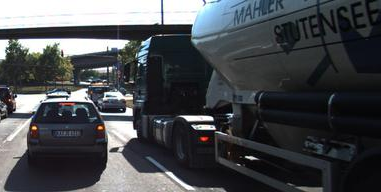
PackNet [18]

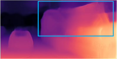
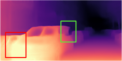
Ours

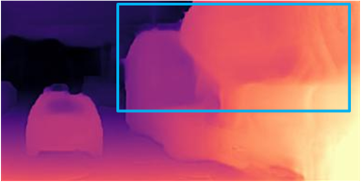
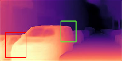
Figure 1: Example of monocular depth estimation. Compared with the SOTA method [18], our method successfully recognizes the object depth from unusual categories (left blue box). At the mean time, our method generates high quality depth map which possesses smooth depth change inside the object region (right green box) and sharp depth edge across object borders (right red box).

Depth estimation is a long-standing problem in computer vision, which is widely used in robotic perception, autonomous driving as well as multimedia applications [36, 13], . Compared with classical geometry-based methods [33, 24] which estimate depth using stereo or sequential images, learning-based methods [12, 11, 23] are able to conduct pixel-wise dense predictions given only a single image as input. However, as the deep neural network requires a large amount of labeled data for training, ideal depth labels are hard to acquire due to the expensive LiDAR sensors as well as the sparse ground truth annotations. Under these circumstances, self-supervised depth estimation [16, 47, 27, 45, 17, 18, 25] has become a new trend that it managed to generate high quality depth maps using only image sequences for supervision.

Despite the impressive results, most current methods use only image representation to model image depth, and seldom consider how the semantic information can be utilized. Image semantics are, however, highly coupled with image representation and scene depth. Therefore it’s necessary to introduce image semantics to assist depth estimation.

We address the benefits of leveraging image semantic guidance in two aspects: on the one hand, it’s highly ill-posed to directly estimate scene depth from images skipping object category information [19]. Specifically, the appeared object size and location in the image, which are commonly regarded as direct depth indicators [19, 10], do not straightly correlate with actual image depth. As shown in the left column of Figure 1, SOTA method [18] failed to infer the depth of a truck with unusual vehicle properties than other cars. On the other hand, image semantics also provide straight clues for object depth. Typically, the semantic borders also correspond to depth borders, and the depth distribution of each individual object is category-specific. For example, objects such as “person” and “traffic sign” possess uniform depth in the scene, while categories “buildings” and “road” exhibit gradual depth change. This raises new challenges for conventional methods. As shown in the right column, [18] produces obvious “bleeding artifacts” [48] in the depth borders, and the abnormal sudden depth changes are also observed inside an continuous object area.

In order to fully exploit the benefits of image semantics for depth estimation, we propose to impose semantic guidances in implicit and explicit ways, respectively. In our framework, we extract semantic features by a semantic segmentation branch, and fuse them with a depth estimation branch at feature level to assist model prediction. In this way, image semantics are combined with image representation to implicitly guide depth estimation. Based on the analysis that the depth distribution is highly related to the semantic categories, we further propose the Semantic-aware Spatial Feature Alignment (SSFA) module, which spatially aligns depth and semantic features via constraining depth distribution to be consistent inside the same category area, while to be different across other categories. During this process, semantic category information is used as external prior to guide the feature alignment. We further propose the semantic-guided ranking loss to explicitly improve the estimated depth map quality. Given semantic labels, we sample a set of cross-edge point quadruplets to explicitly constrain the depth map to be smooth inside the semantic object areas, while to have sharp depth edges across the semantic borders. Different from other edge-based methods [48, 4], we take the impact of erroneous semantic labels into consideration, and propose robust point pair sampling strategy and semantically uncertainty-aware weighting to alleviate semantic label noise. As shown in Figure 1, the proposed implicit and explicit semantic guidances yield accurate depth estimation under different challenging scenarios.

Our contribution can be concluded as follows:

• We address the advantages of leveraging image semantics for both image depth inference and depth map fining. We thus propose implicit and explicit semantic guidances to fulfill the two objectives respectively.

• We propose a novel Semantic-aware Spatial Feature Alignment (SSFA) scheme to effectively guide depth estimation in an implicit manner, and propose the semantic-guided ranking loss to explicitly improve the accuracy of estimated depth map.

• Our method generates consistently superior results across different scenarios and semantic categories, quantitative results on KITTI show that it outperforms the state-of-the-art self-supervised monocular trained methods by a significant margin.

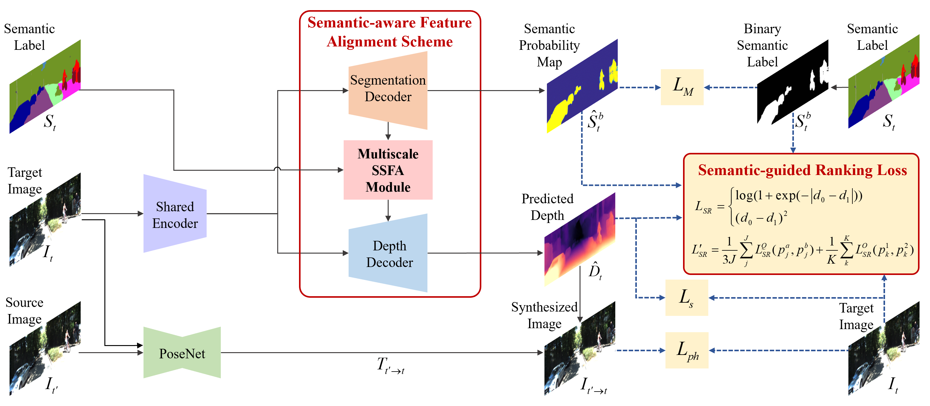
Figure 2: The overview of the proposed architecture. We follow the basic self-supervised depth estimation framework and extend it with both implicit and explicit semantic guidance. The SSFA scheme is proposed to implicitly make depth network semantically aware, while the proposed semantic-guided ranking loss constrains the depth to be consistent with semantic contextual.

2 Related Work

Self-supervised depth estimation. Self-supervised methods cast the depth supervision problem into image-based supervision, which enables learning without depth annotations. As the pioneer methods [16, 14] train depth networks using stereo image pairs, Zhou et al.[47] propose a more generalized pipeline, which enables training with pure image sequences. After that, great progress has been made to improve self-supervised framework in terms of loss, occlusion removal as well as architectures. Yang et al.[44] and Li et al.[25] enhance the photometric loss to be robust towards illumination variance, while Shu et al.[34] propose the feature-metric loss which improves the loss back propagation on low gradient areas. In order to solve the scene occlusion as well as object motion issues during depth training, several methods [47, 17, 2, 38] propose both learning-based and geometric selective mask that filter out the unreliable losses. In order to exploit more information for self-surpervised methods , optical flow is introduced [32, 41, 45] for extra constraints. Pseudo depth is also leveraged as extra prior information [46]. In terms of new self-supervised architectures, Guizilini et al.[18] propose novel packing and unpacking modules which preserves more detailed depth predictions. However, in this paper, for fair comparison, we rule out the influence of new network architectures when comparing with the state-of-the-arts.

Semantic guidance for depth estimation. Semantic segmentation has shown its effectiveness for depth estimation in previous works [7, 19, 4, 31]. The methods can be categorized into two groups according to how image semantics are used. The first group of methods offer implicit semantic guidance via providing feature-level information. Chen et al.[4] generate both depth and semantic maps with a unified scene representation. Guizilini et al.[19] propose to feed the PAC enhanced [35] pre-trained segmentation features for depth estimation. Choi et al.[7] leverage the semantic network and feed the features with cross-propagation and affine-propagation unit. Though we also fuse image depth with semantics in feature level, we align semantic features in a more solid way through our proposed SSFA module, which provides image semantic guidance with distinctly more fidelity and persistence.

The other group of methods use semantic categories to explicitly constrain or supervise depth networks. Ramirez et al.[31] and Chen et al.[4] constrain the smoothness of the depth map using semantic maps. Casser et al.[3] and Klingner et al.[22] handle the dynamic moving object issue via specifying moving areas with semantic object labels, Zhu et al.[48] proposed a stereo-based method which leverages the binary semantic map to generate the edge-aligned pseudo depth labels for direct supervision. Wang et al.[39] propose to learn semantic category-specific depth by a divide-and-conquer strategy. Compared with previous explicit semantic constrains, the proposed semantic-guided ranking loss further takes semantic label noise and prediction uncertainty into account, thus lead to more accurate and reliable depth supervision.

3 The Proposed Method

Self-supervised depth estimation usually takes image triplet $(I_{t-1},I_{t},I_{t+1})$ as input, where $I_{t}$ is the target image and $I_{t^{{}^{\prime}}}\in\{I_{t-1},I_{t+1}\}$ belongs to the source images. During training, $I_{t}$ is fed into the depth network $f_{D}$ to get the predicted depth $\hat{D}_{t}\in\mathbb{R}^{H\times W}$, where $H$ and $W$ are the image height and width. $(I_{t},I_{t^{{}^{\prime}}})$ are put into the motion network to get the relative motion $T_{t^{{}^{\prime}}\rightarrow t}$. Then, the synthesized image $I_{t^{{}^{\prime}}\rightarrow t}$ can be computed with $I_{t}$, $\hat{D}_{t}$ and $T_{t^{{}^{\prime}}\rightarrow t}$ [47]. The depth network is trained by back-propagating the photometric loss between the synthesized images $I_{t^{{}^{\prime}}\rightarrow t}$ and the target image $I_{t}$, as proposed by Godard et al.[17]

$$L_{ph}(I_{t},I_{t^{{}^{\prime}}\rightarrow t})=\min_{t^{\prime}}(\frac{\alpha}{2}(1-\operatorname{SSIM}\left(I_{t},I_{t^{\prime}\rightarrow t}\right))$$ (1)

$$+(1-\alpha)\left\|I_{t}-I_{t^{\prime}\rightarrow t}\right\|_{1}),$$

where SSIM denotes the structural similarity index [42], $\alpha$ refers to the weighting factor which is commonly set to $0.85$ [17, 16, 47]. The first-order depth smoothness loss $L_{s}$ is also set with the weighting factor of $10^{-3}$ [16].

In this paper, we follow the basic self-supervised framework but extend it with implicit and explicit semantic guidances for accurate depth estimation. During depth inferring, we introduce a SSFA module to incorporate image semantics, which implicitly makes the estimated depth semantically aware. We further explicitly constrain the estimated depth map with semantic-guided ranking loss, and improve the accuracy and reliability of our predicted depth map. The overview of our model is shown in Figure 2.

3.1 Semantic-aware Feature Alignment Scheme

We enhance the depth estimation performance implicitly by providing semantic feature representations to the depth network. Thus, a semantic branch is proposed to offer semantic category-level information in a multi-scale scheme, see Section 3.1.1. Consider the semantic and depth features are from the different task domains, we align the features by the proposed semantic-aware spatial feature alignment (SSFA) module, utilizes external semantic category-level labels for better semantic guidance, see Section 3.1.2.

3.1.1 Semantic Multi-task Scheme

We extend the general self-supervised depth estimation framework by add an extra semantic branch $f_{S}$, which shares the same encoder with the depth network, as shown in the top of Figure 3. Given the input image $I$, a semantic probability map $\hat{S}^{b}\in[0,1]^{H\times W}$ is generated and supervised by the given binary semantic label $S^{b}\in\{0,1\}^{H\times W}$

$$L_{M}=BCELoss(\hat{S}^{b},S^{b}),$$ (2)

where $BCELoss(\cdot)$ denotes the binary cross-entropy loss. The semantic labels can be either groundtruth or pre-computed labels from other methods, we use the latter [49] in our experiments due to the lack of semantic groundtruth annotations. Let $S\in\mathbb{M}^{H\times W}$ the full semantic label, where $\mathbb{M}$ is the integers denoting the semantic categories. We generate the binary semantic label $S^{b}$ by specifying foreground objects of the given $S$. The reasons for generating the binary semantic map are twofold, 1) it provides comparable informative semantic features to the depth branch as the full semantic map does [1], 2) when using pre-computed semantic labels, cross-domain trained segmentation method [49] achieves much higher mIoU for binary predictions than full category predictions, which indicates that binary labels are more reliable as the input. Experimental details can be found on Section 4.6. The semantic branch is trained together with the depth network, and provides latent semantic features to the depth decoding layers in a multi-scale manner, as shown in Figure 3.

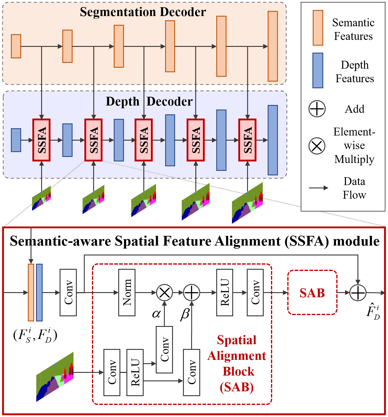
Figure 3: The proposed semantic-aware feature alignment scheme. We propose an extra semantic branch to implicitly offer semantic information to the depth network in a multi-scale manner. During the process, a semantic-aware spatial alignment (SSFA) module is proposed which improves the fusion of depth and semantic features via conducting spatial operations learned from the semantic guidance.

3.1.2 Semantic-aware Spatial Feature Alignment

Since the semantic and depth features are from different task domains, the simple fusions (direct concatenation or convolution, .) do not fully exploit the potential of image semantics for depth estimation. In this paper, consider the depth distribution of the scene is category-specific, we deduce the distribution of depth features should also be category-specific. Thus, we propose the Semantic-aware Spatial Feature Alignment (SSFA) module, which takes the semantic labels as external prior, to align the features and make them conform to the category-specific distributions, via semantic-aware spatial normalization operations.

As shown in Figure 3, during network training, we have multi-scale semantic features $F^{i}_{S}\in\mathbb{R}^{C_{i}\times H\times W}$ and depth features $F^{i}_{D}\in\mathbb{R}^{C_{i}\times H\times W}$, where $C_{i}$ denotes the channels of the feature block and $i\in\{0,1,2,3,4\}$. We propose $5$ SSFA modules corresponding to the number of scales. For each input pair $(F^{i}_{S},F^{i}_{D})$, the corresponding SSFA module outputs the aligned feature $\hat{F}^{i}_{D}$ as the input of the next scale.

For each SSFA module, we propose two semantic-aware spatial alignment blocks (SAB) with residual connection as shown in the bottom of Figure 3. The SSFA module first fuses the two features together and then put the coarsely fused feature $F^{i}_{S+D}$ into the two blocks. Given an input feature $F$ to the spatial alignment block, the block first normalize the input feature in the channel-wise manner, then spatially align the normalized feature $F_{norm}$ with the learned category-specific multiplicative factor $\alpha$ and additive factor $\beta$, as inspired by [30, 40]

$$F_{aligned}=\alpha\otimes F_{norm}\oplus\beta,$$ (3)

where $\otimes$ and $\oplus$ denote element-wise multiplication and addition, $\alpha$ and $\beta$ are learned from the semantic labels via simple conventional layers. After the multi-level processing with the proposed SSFA modules, the output features $\hat{F}^{i}_{D}$ are endowed with better representation capabilities that both semantic and depth features are well aligned by the category-level semantic guidance.

3.2 Semantic-guided Ranking Loss

In this section, we explicitly constrain the generated depth map to be consistent inside semantic categories and to be sharp cross the category borders. We resort to the ranking loss [5] for it directly constrains the depth differences, which is more suitable to constrain depth sharpness/smoothness. Different from the existing depth ranking loss [5, 43] which use the point pair depth similarity to specify the maximize or minimize operation of depth difference, we instead propose a semantic-guided ranking loss, which maximize/minimize the point pair depth difference according to their semantic belongings. For a sampled point pair $(p_{0},p_{1})$ with depth $(d_{0},d_{1})$, the semantic-guided ranking loss $L_{SR}$ can be formulated as

$$L_{SR}\left(p_{0},p_{1}\right)=\left\{\begin{array}[]{ll}\log\left(1+\exp\left(-|d_{0}-d_{1}|\right)\right),&\ell=1\\ \left(d_{0}-d_{1}\right)^{2},&\ell=0\end{array}\right.$$ (4)

where $\ell$ is the semantic belonging indicator denoting the semantic relationship between point pairs

$$\ell=\left\{\begin{array}[]{ll}1,&S^{b}(p_{0})\neq S^{b}(p_{1})\\ 0,&S^{b}(p_{0})=S^{b}(p_{1})\end{array}\right.$$ (5)

where $S_{b}$ is the binary semantic label. If $(p_{0},p_{1})$ lie across the semantic border, $\ell=1$, we constrain the depth difference between $(d_{0},d_{1})$ to be large for sharp depth edges. Otherwise, we minimize the depth difference between $(d_{0},d_{1})$ to make the depth smooth inside the same semantic category. Consider the proposed loss relies explicitly on the semantic borders, little noise on the semantic labels will cause erroneous constrains for the predicted depth. To address this problem, a cross-border point pair sampling strategy (see Section 3.2.1) and a semantically uncertainty-aware weighting factor (see Section 3.2.2) is proposed which consider the noise of input semantic labels.

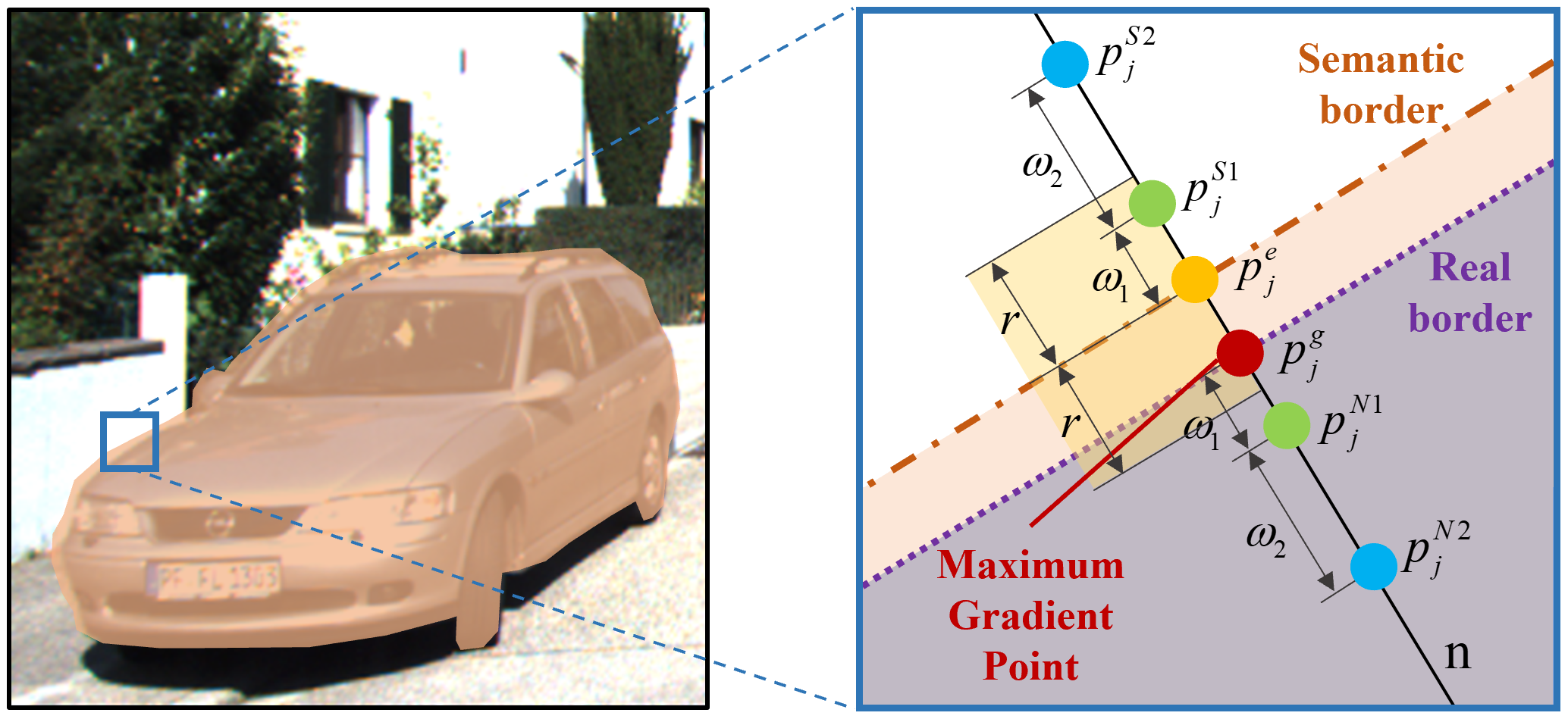
Figure 4: The proposed semantic-guided edge sampling strategy. For every edge point $p_{j}^{e}$, we sample a point quadruplet $Q_{e}=\{p^{S1}_{j},p^{S2}_{j},p^{N1}_{j},p^{N2}_{j}\}$ along orthogonal line $\mathbf{n}$. To find the real border, we search the max gradient point $p_{j}^{g}$ along $\mathbf{n}$ in range $[-r,r]$, and make the cross-border point pair $(p^{S1}_{j},p^{N1}_{j})$ to clamp $p_{j}^{e}$ and $p_{j}^{g}$.

3.2.1 Cross-border Point Pair Sampling Strategy

Inspired by [43], we propose to sample a set of point quadruplets $Q=\{q_{j}\}_{j=1}^{J}$ on the semantic borders to compute the ranking loss, where $J$ is the number of edge points. We first compute the edge map of the binary semantic label, and for every edge point $p_{j}^{e}$, we sample a quadruplet $q_{j}\in Q$, $q_{j}=\{p^{S1}_{j},p^{S2}_{j},p^{N1}_{j},p^{N2}_{j}\}$ which contains $4$ co-linear points lying along the orthogonal line $\mathbf{n}$ crossing the edge point. As shown in Figure 4, point $p^{S1}_{j}$ and $p^{S2}_{j}$ lie on one side of $p_{j}^{e}$, then point $p^{N1}_{j}$ and $p^{N2}_{j}$ lie on the other. Totally three point pairs $[(p^{S1}_{j},p^{S2}_{j}),(p^{S1}_{j},p^{N1}_{j}),(p^{N1}_{j},p^{N2}_{j})]$ are generated for computing the ranking loss.

While $(p^{S1}_{j},p^{N1}_{j})$ is supposed to be the cross-border point pair, the edge point $p_{j}^{e}$ from noisy semantic labels are not reliable to represent the real object border. In this section, we solve this problem by incorporating image gradient as another clue to detect real object borders, for the object border points usually possess the largest gradient value in the local area. We search the maximum image gradient point $p_{j}^{g}$ along the line $\mathbf{n}$, within a small distance range $r$ to the edge point $p_{j}^{e}$. As shown in Figure 4, when sampling the cross-border point, we set $(p^{S1}_{j},p^{N1}_{j})$ to clamp both $p_{j}^{g}$ and $p_{j}^{e}$ to make the sampled points across both semantic and image gradient border. The margin pixel $\omega_{1}$ is set to $1$ for tight clamping. The distance range $r$ is set to $[-5,5]$ empirically, in order to strike a balance between finding the real borders and making the sampled pairs close to the borders. For point $p^{S2}_{j}$ and $p^{N2}_{j}$, they are sampled besides the $p^{S1}_{j}$ and $p^{N1}_{j}$ respectively, within a distance range $\omega_{2}$ which is set to $[2.5,10]$. For each input image, we select all edge points and feed all corresponding quadruplets to compute the ranking loss in Equation 4. Besides the cross border point quadruplets set $Q$, we also randomly sample a point pair set $O=\{(p^{1}_{k},p^{2}_{k})\}_{k=1}^{K}$, whose point pairs lie inside the semantic borders, to constrain the depth smoothness in a broader range.

Method	Training	Abs Rel	Sq Rel	RMSE	RMSElog	$\delta<1.25$	$\delta<1.25^{2}$	$\delta<1.25^{2}$
Zhou [47]	M	0.183	1.595	6.709	0.270	0.734	0.902	0.959
Mahjourian [27]	M	0.163	1.240	6.220	0.250	0.762	0.916	0.968
GeoNet [45]	M	0.155	1.296	5.857	0.233	0.793	0.931	0.973
DDVO [37]	M	0.151	1.257	5.583	0.228	0.810	0.936	0.974
CC [32]	M	0.140	1.070	5.326	0.217	0.826	0.941	0.975
EPC++ [26]	M	1.029	1.070	5.350	0.216	0.816	0.941	0.976
GLNet [6]	M	0.135	1.070	5.230	0.210	0.841	0.948	0.980
Monodepth2 [17]	M	0.115	0.903	4.863	0.193	0.877	0.959	0.981
PackNet [18]	M	0.111	0.785	4.601	0.189	0.878	0.960	0.982
Johnston [21]	M	0.106	0.861	4.699	0.185	0.889	0.962	0.982
Casser [3]	M+Inst	0.141	1.026	5.291	0.215	0.816	0.945	0.979
Chen [4]	M+Sem	0.118	0.905	5.096	0.211	0.839	0.945	0.977
Ochs [29]	D+Sem	0.116	0.945	4.916	0.208	0.861	0.952	0.968
Guizilini [19] - PackNet	M+Sem	0.102	0.698	4.381	0.178	0.896	0.964	0.984
Guizilini [19] - Res50	M+Sem	0.113	0.831	4.663	0.189	0.878	0.971	0.983
Ours	M+Sem	0.103	0.709	4.471	0.180	0.892	0.966	0.984
Casser (+ref.) [3]	M+Inst	0.109	0.825	4.750	0.187	0.874	0.958	0.983
GLNet (+ref.) [6]	M	0.099	0.796	4.743	0.186	0.884	0.955	0.979
Ours (+ref.)	M+Sem	0.095	0.666	4.252	0.172	0.905	0.968	0.984

Table 1: Quantitative results on KITTI 2015. The best results are in bold and the second best results are underlined. “M” refer to self-supervision methods using monocular images only. “Inst” and “Sem” denote methods which leverage instance or semantic segmentation information. “-Res50” refers to the method which uses Resnet-50 as the backbone encoder. “+ref.” represents using the online refinement operation. All results are reported within range $[0m,80m]$. The metrics marked in blue mean “lower is better”, while these in red refer to “higher is better”. Our method outperforms the state-of-the-arts in most metrics by significant margins.

3.2.2 Semantically Uncertainty-aware Weighting

Although the cross-border sampling strategy in Section 3.2.1 heuristically constrains the point pairs to cross the real object border, it will fail when the pre-computed segmentation mask deviates significantly from the groundtruth. To address this problem, we propose a semantically uncertainty-aware weighting factor $\gamma$ for Equation 4, which evaluate the quality of the input quadruplet $q_{j}$ by leveraging semantic probabilities of the cross-border point pair. The semantic probability map $\hat{S}_{b}$ is generated by the semantic branch $f_{S}$. Though not being the ground truth probability, it indeed reflects the semantic uncertainties across different areas. Thus when computing the ranking loss of the three point pairs inside $q_{j}$, the weighted loss $L^{Q}_{SR}(p^{a}_{j},p^{b}_{j})$ is

$$L^{Q}_{SR}(p^{a}_{j},p^{b}_{j})=\gamma\cdot L_{SR}(p^{a}_{j},p^{b}_{j}),$$ (6)

where $p_{j}^{a},p_{j}^{b}\in q_{j}$, the weighting value $\gamma\in[\frac{1}{e},1]$ is decided by the differences of semantic probabilities between the point pair $p^{S1}_{j}$ and $p^{N1}_{j}$

$$\gamma=\exp(-1/\max(\frac{\hat{S}_{b}(p^{S1}_{j})}{\hat{S}_{b}(p^{N1}_{j})},\frac{\hat{S}_{b}(p^{N1}_{j})}{\hat{S}_{b}(p^{S1}_{j})})).$$ (7)

This means the more confident the semantic network is to its predicted cross-border points, the larger weight will be assigned to the three ranking losses. Note that for the points pairs $O$, $L^{O}_{SR}(p^{1}_{k},p^{2}_{k})=L_{SR}(p^{1}_{k},p^{2}_{k})$. The final ranking loss $L^{\prime}_{SR}$ can be formulated as

$$L^{\prime}_{SR}=\frac{1}{3J}\sum_{j}^{J}L^{Q}_{SR}(p^{a}_{j},p^{b}_{j})+\frac{1}{K}\sum_{k}^{K}L^{O}_{SR}(p^{1}_{k},p^{2}_{k})$$ (8)

3.3 Final Loss

The final loss of the whole pipeline can be formulated as

$$L=L_{ph}+L_{M}+\delta_{s}L_{s}+\delta_{r}L^{\prime}_{SR},$$ (9)

where $\delta_{s}$ is set to $0.001$ for common practice [17], and $\delta_{r}$ is set to $0.001$ empirically that it strikes a balance between overall performance and depth sharpness/smoothness.

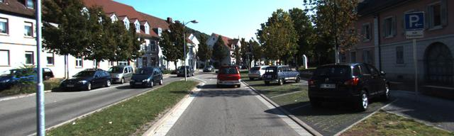
Input

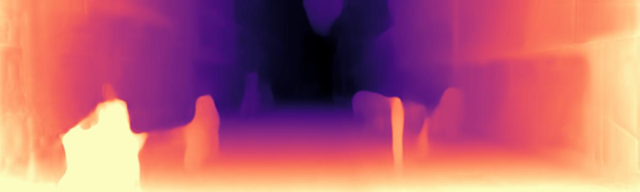
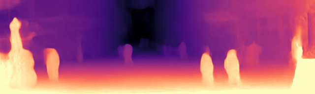
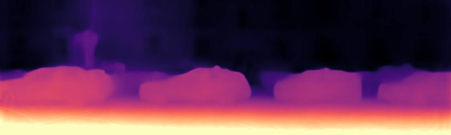
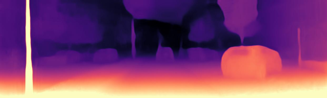
Monodepth2 [17]

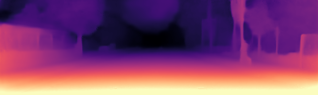
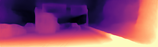
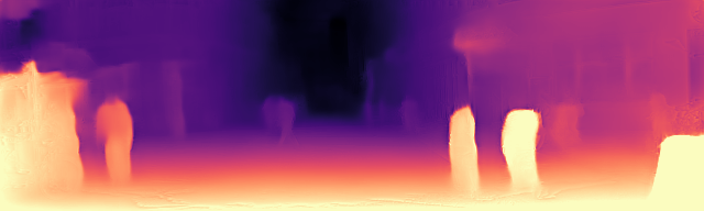
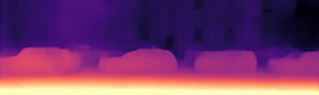
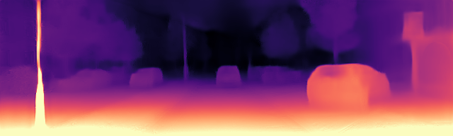
PackNet [18]

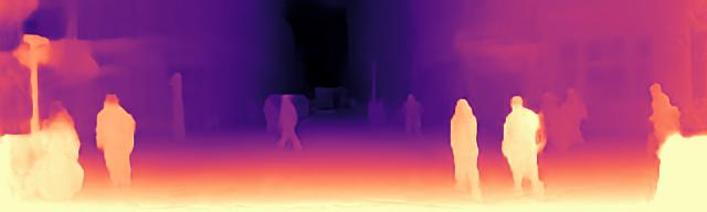
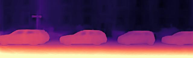
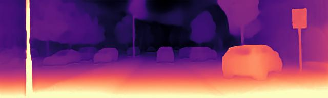
Ours

Figure 5: Qualitative comparison on KITTI. Our method shows its superiority in producing better category-level depth predictions, and generates accurate depth predictions which are smooth inside the objects and sharp across object borders.

4 Experiments

In this section, we conduct comprehensive comparisons to demonstrate the superiority of our method toward the state-of-the-arts, and validate the generalization ability of the proposed method in leveraging semantic information.

4.1 Experimental Settings

Dataset. We use the KITTI 2015 [15] dataset with Eigen’s split [12] and Zhou’s [47] pre-preprocessing strategy, which leads to 39810 training images and 697 testing images. For the training of the semantic branch, we only use the pre-computed semantic maps from an off-the-shelf model [49] for supervision. The model is pre-trained on Cityscape [8] (CS) and Mapillary Vistas dataset [28] (V). We mainly use the model fine-tuned on 200 KITTI (K) labeled images to generate the dataset $\mathbf{Sem}_{CS+V+K}$. Consider the real world scenarios, we also maintain another dataset $\mathbf{Sem}_{CS+V}$ without fine-tunning on KITTI, to validate the feasibility of using the precomputed labels trained from cross-domain datasets. We follow the practice of [48] to generate the binary semantic maps.

Implementation Details. We build our method on Monodepth2 [17] with ResNet-50 [20] pre-trained on the ImageNet [9] as backbone. The model is trained on a single NVIDIA Tesla V100 GPU with batch size of 12. The learning rate is set to $10^{-4}$ and divided by $10$ for every $15$ epochs. After the network converges, we select the model of epoch 20 for testing. The input image size is set to $192\times 640$ following [17], and we compare our method with others on the same image resolution. We conduct online refinement following the practice of [3, 6, 34] with batch size of $1$. The online refinement is performed $20$ iterations on each test image, there is no data augmentation during this process. During testing, the network generates depth from the input image, and the semantic label is used to guide the feature alignment of the depth and semantic branches.

4.2 Results on KITTI

We compare the proposed method with state-of-the-art monocular trained depth estimation methods on KITTI 2015 [15], the quantitative results are shown in Table 1. Note that the PackNet-based implementation of Guizilini et al.[19] is $0.102$ in AbsRel. However, PackNet [18] alone takes more than 120M parameters for training, which is not applicable under certain circumstances with limited computation resources. Thus, we select the general Resnet-50 as backbone, which is also the same as our method for fair comparison. Our method outperforms state-of-the-art methods by a large margin on most evaluation metrics. The qualitative results are shown in Figure 5. The superiority of our method are illustrated in two aspects. Firstly, our method outperforms others in understanding depth from the category-level perspective. For instance, it successfully infers the correct depth on “train” and “traffic sign” area than other methods in the row $1\sim 2$ of Figure 5. Secondly, our method predicts high quality depth which is smooth inside object area (as the rider on row $3$), and is sharp across the object borders (as the borders of people, cars and traffic signs in row $4\sim 6$). More results can be found in the supplementary material.

Method	SSFA	SRL	Abs Rel	Sq Rel	RMSE	RMSElog	$\delta\leq 1.25$	$\pagecolor{my_red}\delta\leq 1.25^{2}$	$\pagecolor{my_red}\delta\leq 1.25^{2}$
Baseline	✗	✗	0.110	0.830	4.639	0.187	0.884	0.962	0.982
Baseline + SSFA	✓	✗	0.107	0.777	4.583	0.183	0.889	0.963	0.983
Baseline + SRL	✗	✓	0.107	0.766	4.583	0.184	0.887	0.963	0.983
Baseline + SSFA + SRL	✓	✓	0.103	0.709	4.471	0.180	0.892	0.966	0.984

Table 2: Ablation experiments. We show the results of several ablated versions of our method on KITTI 2015 [15]. “SSFA” denotes the proposed SSFA scheme, and “SRL” refers to the semantic ranking loss. The best results are in bold.

4.3 Ablation Study

We evaluate the effectiveness of the proposed modules in Table 2 by comparing the different versions of our method. We see that the baseline model performs the worst among all, and our proposed contributions improve consistently upon the baseline. When combined together, both contributions lead to a significant improvement of the performance.

4.4 Category-specific Depth Improvement

To further analysis the category-level improvements, we evaluate the improvement of depth predictions with respect to their semantic labels. Due to the absence of semantic groundtruth, we use the fine-tuned predicted labels $\mathbf{Sem}_{CS+V+K}$ to specify the semantic area. We compare our method with the baseline model [17], with AbsRel as the evaluation metric. As shown in Figure 6, our method shows improvements towards most of the categories, including not only the foreground categories (traffic signs, person, cars, .), but also the background categories (sky, fence, wall, .) which can not be directly seen from the binary mask. It indicates that the semantic features provided by the binary mask are capable to offer rich contextual information with the guidance of the SSFA.

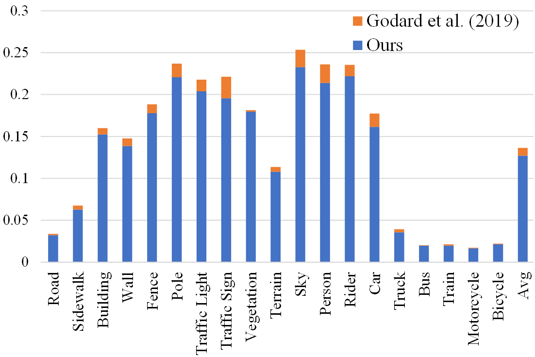
Figure 6: Category-specific depth improvement. We compare our method (blue) with the baseline (orange) using the metric of AbsRel. The rightmost is the average performance, which is the mean value of all categories’ performance. Our method improves consistently across most categories, including the foreground (person, rider, traffic sign, .) and the background (sky, fence, wall, .) classes.

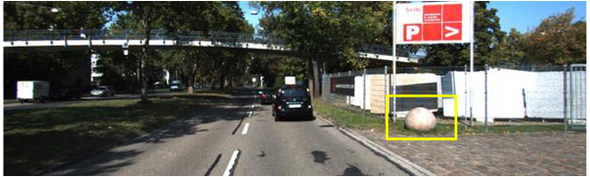
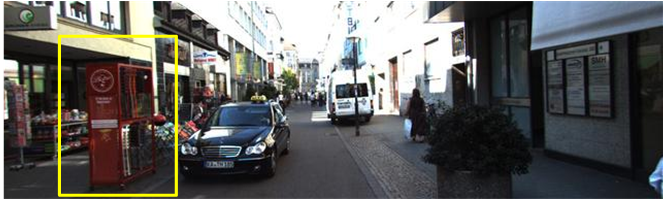
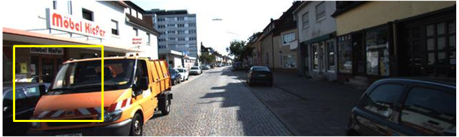
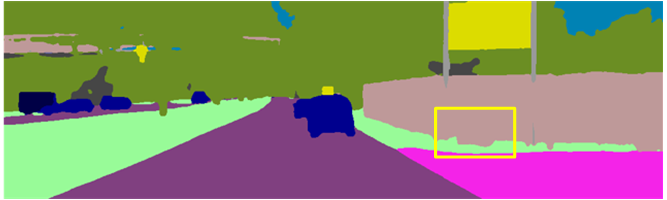
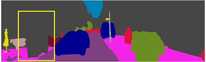
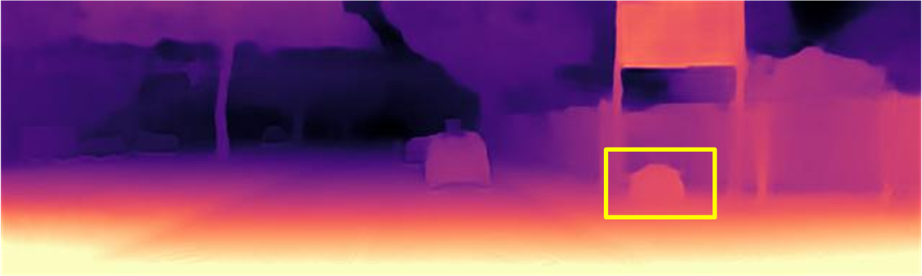
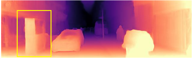
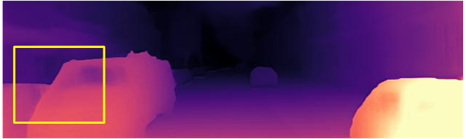
Figure 7: Depth from erroneous segmentation labels. Despite different types of semantic degradation, our method still produce accurate depth maps.

4.5 Performance on Noisy Semantic Labels

Due to the desperately lack of groundtruth semantic labels on real world scenarios, the noisy semantic inputs are inevitable during both training and testing phrase. We validate the effectiveness of our method in sampling point pairs across the real object borders (see Section 3.2.1). We use the pre-computed semantic label as guidance, and compare the proposed semantic-guided sampling strategy with the direct strategy which samples directly beside the edge points. We calculate the ratio of real cross-border points to all sampled pairs, using KITTI Semantics dataset [15] as groundtruth. The quantitative results are shown in Table 3. Our sampling strategy improves upon the direct sampling strategy by a significant margin of $19.9\%$, which shows its great superiority in finding the real borders in the local area.

Sampling Strategy	Direct	The Proposed
Accuracy (%)	55.3	75.2

Table 3: The sampling accuracy of different strategies. Our semantic-guided sampling strategy outperforms the direct method by a significant margin of $19.9\%$.

During testing, we validate that our method can successfully handle erroneous semantic inputs as shown in Figure 7. For the input semantic labels, in the first row the stone is mistaken as the wall, in the second row the cabinet is not labeled and in the third row, the boundary of the left car is extremely imprecise. Despite the erroneous semantic predictions, our method still succeed in performing accurate depth predictions of the true scene structure.

Dataset	mIoUFull	mIoUBi	Abs Rel	RMSE	$\delta\leq 1.25$
$\mathbf{Sem}_{CS+V}$	67.73	93.54	0.105	4.516	0.890
$\mathbf{Sem}_{CS+V+K}$	79.90	94.74	0.103	4.471	0.892

Table 4: Performance on different datasets. The binary segmentation IoU (mIoU_Bi) differs a little across different datasets, and our model achieves comparable results on cross-domain generated semantic labels.

4.6 Study on Cross-domain Semantic Labels

Although fine-tuned only on $200$ KITTI semantic labels, the generated semantic dataset $\mathbf{Sem}_{CS+V+K}$ is still guided by groundtruth information. To further validate the generalization ability, we train our model with semantic dataset $\mathbf{Sem}_{CS+V}$, which is acquired from totally cross-domain trained semantic model. As shown in Table 4, we found an interesting phenomenon that although the full segmentation mIoU (mIoU_Full) of $\mathbf{Sem}_{CS+V}$ is obviously worse than that of $\mathbf{Sem}_{CS+V+K}$, their binary mIoU (mIoU_Bi) is very close to each other ($93.54\%$ to $94.74\%$). It validates the advantage of the binary semantic maps, with which the performance of both semantic branch and semantic-guided sampling are less influenced by cross-domain predictions. At the meantime, our model trained on the cross-domain semantic dataset $\mathbf{Sem}_{CS+V}$ generalizes well, for its performance is only slightly behind with the one trained on $\mathbf{Sem}_{CS+V+K}$, while still outperforms the state-of-the-art methods [18, 17, 21].

5 Conclusion

In this paper, we improve self-supervised depth estimation via leveraging both implicit and explicit semantic guidance. We propose a semantic-guided spatial feature alignment scheme to implicitly model the semantic category-level information for depth estimation. And we propose a semantic-guided ranking loss to explicitly constrain the depth map’s accuracy regarding to specific object categories. Extensive experiments show the superiority of the method. In future research, we plan to leverage the semantic information for depth refinement, to further improve the performance after the initial predictions.

References

- [1] Anonymous. Semantic-guided representation enhancement for self-supervised monocular trained depth estimation. In Submitted to International Conference on Learning Representations, 2021. under review.
- [2] Jiawang Bian, Zhichao Li, Naiyan Wang, Huangying Zhan, Chunhua Shen, Ming-Ming Cheng, and Ian Reid. Unsupervised scale-consistent depth and ego-motion learning from monocular video. In Advances in Neural Information Processing Systems, pages 35–45, 2019.
- [3] Vincent Casser, Soeren Pirk, Reza Mahjourian, and Anelia Angelova. Depth prediction without the sensors: Leveraging structure for unsupervised learning from monocular videos. In Proceedings of the AAAI Conference on Artificial Intelligence, volume 33, pages 8001–8008, 2019.
- [4] Po-Yi Chen, Alexander H Liu, Yen-Cheng Liu, and Yu-Chiang Frank Wang. Towards scene understanding: Unsupervised monocular depth estimation with semantic-aware representation. In Proceedings of the IEEE Conference on Computer Vision and Pattern Recognition, pages 2624–2632, 2019.
- [5] Weifeng Chen, Zhao Fu, Dawei Yang, and Jia Deng. Single-image depth perception in the wild. In Advances in neural information processing systems, pages 730–738, 2016.
- [6] Yuhua Chen, Cordelia Schmid, and Cristian Sminchisescu. Self-supervised learning with geometric constraints in monocular video: Connecting flow, depth, and camera. In Proceedings of the IEEE International Conference on Computer Vision, pages 7063–7072, 2019.
- [7] Jaehoon Choi, Dongki Jung, Donghwan Lee, and Changick Kim. Safenet: Self-supervised monocular depth estimation with semantic-aware feature extraction. arXiv preprint arXiv:2010.02893, 2020.
- [8] Marius Cordts, Mohamed Omran, Sebastian Ramos, Timo Rehfeld, Markus Enzweiler, Rodrigo Benenson, Uwe Franke, Stefan Roth, and Bernt Schiele. The cityscapes dataset for semantic urban scene understanding. In Proceedings of the IEEE conference on computer vision and pattern recognition, pages 3213–3223, 2016.
- [9] Jia Deng, Wei Dong, Richard Socher, Li-Jia Li, Kai Li, and Li Fei-Fei. Imagenet: A large-scale hierarchical image database. In 2009 IEEE conference on computer vision and pattern recognition, pages 248–255. Ieee, 2009.
- [10] Tom van Dijk and Guido de Croon. How do neural networks see depth in single images? In Proceedings of the IEEE International Conference on Computer Vision, pages 2183–2191, 2019.
- [11] David Eigen and Rob Fergus. Predicting depth, surface normals and semantic labels with a common multi-scale convolutional architecture. In Proceedings of the IEEE international conference on computer vision, pages 2650–2658, 2015.
- [12] David Eigen, Christian Puhrsch, and Rob Fergus. Depth map prediction from a single image using a multi-scale deep network. In Advances in neural information processing systems, pages 2366–2374, 2014.
- [13] A Gaidon, Q Wang, Y Cabon, and E Vig. Virtual worlds as proxy for multi-object tracking analysis. In CVPR, 2016.
- [14] Ravi Garg, Vijay Kumar Bg, Gustavo Carneiro, and Ian Reid. Unsupervised cnn for single view depth estimation: Geometry to the rescue. In European conference on computer vision, pages 740–756. Springer, 2016.
- [15] Andreas Geiger, Philip Lenz, and Raquel Urtasun. Are we ready for autonomous driving? the kitti vision benchmark suite. In 2012 IEEE Conference on Computer Vision and Pattern Recognition, pages 3354–3361. IEEE, 2012.
- [16] Clément Godard, Oisin Mac Aodha, and Gabriel J Brostow. Unsupervised monocular depth estimation with left-right consistency. In Proceedings of the IEEE Conference on Computer Vision and Pattern Recognition, pages 270–279, 2017.
- [17] Clément Godard, Oisin Mac Aodha, Michael Firman, and Gabriel J Brostow. Digging into self-supervised monocular depth estimation. In Proceedings of the IEEE International Conference on Computer Vision, pages 3828–3838, 2019.
- [18] Vitor Guizilini, Rares Ambrus, Sudeep Pillai, Allan Raventos, and Adrien Gaidon. 3d packing for self-supervised monocular depth estimation. In Proceedings of the IEEE/CVF Conference on Computer Vision and Pattern Recognition, pages 2485–2494, 2020.
- [19] Vitor Guizilini, Rui Hou, Jie Li, Rares Ambrus, and Adrien Gaidon. Semantically-guided representation learning for self-supervised monocular depth. arXiv preprint arXiv:2002.12319, 2020.
- [20] Kaiming He, Xiangyu Zhang, Shaoqing Ren, and Jian Sun. Deep residual learning for image recognition. In Proceedings of the IEEE conference on computer vision and pattern recognition, pages 770–778, 2016.
- [21] Adrian Johnston and Gustavo Carneiro. Self-supervised monocular trained depth estimation using self-attention and discrete disparity volume. In Proceedings of the IEEE/CVF Conference on Computer Vision and Pattern Recognition, pages 4756–4765, 2020.
- [22] Marvin Klingner, Jan-Aike Termöhlen, Jonas Mikolajczyk, and Tim Fingscheidt. Self-supervised monocular depth estimation: Solving the dynamic object problem by semantic guidance. arXiv preprint arXiv:2007.06936, 2020.
- [23] Bo Li, Chunhua Shen, Yuchao Dai, Anton Van Den Hengel, and Mingyi He. Depth and surface normal estimation from monocular images using regression on deep features and hierarchical crfs. In Proceedings of the IEEE conference on computer vision and pattern recognition, pages 1119–1127, 2015.
- [24] Rui Li, Dong Gong, Jinqiu Sun, Yu Zhu, Ziwei Wei, and Yanning Zhang. Robust and accurate hybrid structure-from-moti. In 2019 IEEE International Conference on Image Processing (ICIP), pages 494–498. IEEE, 2019.
- [25] Rui Li, Xiantuo He, Yu Zhu, Xianjun Li, Jinqiu Sun, and Yanning Zhang. Enhancing self-supervised monocular depth estimation via incorporating robust constraints. In Proceedings of the 28th ACM International Conference on Multimedia, pages 3108–3117, 2020.
- [26] Chenxu Luo, Zhenheng Yang, Peng Wang, Yang Wang, Wei Xu, Ram Nevatia, and Alan Yuille. Every pixel counts++: Joint learning of geometry and motion with 3d holistic understanding. arXiv preprint arXiv:1810.06125, 2018.
- [27] Reza Mahjourian, Martin Wicke, and Anelia Angelova. Unsupervised learning of depth and ego-motion from monocular video using 3d geometric constraints. In Proceedings of the IEEE Conference on Computer Vision and Pattern Recognition, pages 5667–5675, 2018.
- [28] Gerhard Neuhold, Tobias Ollmann, Samuel Rota Bulò, and Peter Kontschieder. The mapillary vistas dataset for semantic understanding of street scenes. In International Conference on Computer Vision (ICCV), 2017.
- [29] Matthias Ochs, Adrian Kretz, and Rudolf Mester. Sdnet: Semantically guided depth estimation network. In German Conference on Pattern Recognition, pages 288–302. Springer, 2019.
- [30] Taesung Park, Ming-Yu Liu, Ting-Chun Wang, and Jun-Yan Zhu. Semantic image synthesis with spatially-adaptive normalization. In Proceedings of the IEEE Conference on Computer Vision and Pattern Recognition, pages 2337–2346, 2019.
- [31] Pierluigi Zama Ramirez, Matteo Poggi, Fabio Tosi, Stefano Mattoccia, and Luigi Di Stefano. Geometry meets semantics for semi-supervised monocular depth estimation. In Asian Conference on Computer Vision, pages 298–313. Springer, 2018.
- [32] Anurag Ranjan, Varun Jampani, Lukas Balles, Kihwan Kim, Deqing Sun, Jonas Wulff, and Michael J Black. Competitive collaboration: Joint unsupervised learning of depth, camera motion, optical flow and motion segmentation. In Proceedings of the IEEE Conference on Computer Vision and Pattern Recognition, pages 12240–12249, 2019.
- [33] Johannes L Schonberger and Jan-Michael Frahm. Structure-from-motion revisited. In Proceedings of the IEEE Conference on Computer Vision and Pattern Recognition, pages 4104–4113, 2016.
- [34] Chang Shu, Kun Yu, Zhixiang Duan, and Kuiyuan Yang. Feature-metric loss for self-supervised learning of depth and egomotion. arXiv preprint arXiv:2007.10603, 2020.
- [35] Hang Su, Varun Jampani, Deqing Sun, Orazio Gallo, Erik Learned-Miller, and Jan Kautz. Pixel-adaptive convolutional neural networks. In Proceedings of the IEEE Conference on Computer Vision and Pattern Recognition, pages 11166–11175, 2019.
- [36] Ulrich Viereck, Andreas ten Pas, Kate Saenko, and Robert Platt. Learning a visuomotor controller for real world robotic grasping using simulated depth images. arXiv preprint arXiv:1706.04652, 2017.
- [37] Chaoyang Wang, José Miguel Buenaposada, Rui Zhu, and Simon Lucey. Learning depth from monocular videos using direct methods. In Proceedings of the IEEE Conference on Computer Vision and Pattern Recognition, pages 2022–2030, 2018.
- [38] Guangming Wang, Hesheng Wang, Yiling Liu, and Weidong Chen. Unsupervised learning of monocular depth and ego-motion using multiple masks. In 2019 International Conference on Robotics and Automation (ICRA), pages 4724–4730. IEEE, 2019.
- [39] Lijun Wang, Jianming Zhang, Oliver Wang, Zhe Lin, and Huchuan Lu. Sdc-depth: Semantic divide-and-conquer network for monocular depth estimation. In Proceedings of the IEEE/CVF Conference on Computer Vision and Pattern Recognition, pages 541–550, 2020.
- [40] Xintao Wang, Ke Yu, Chao Dong, and Chen Change Loy. Recovering realistic texture in image super-resolution by deep spatial feature transform. In Proceedings of the IEEE conference on computer vision and pattern recognition, pages 606–615, 2018.
- [41] Yang Wang, Peng Wang, Zhenheng Yang, Chenxu Luo, Yi Yang, and Wei Xu. Unos: Unified unsupervised optical-flow and stereo-depth estimation by watching videos. In Proceedings of the IEEE Conference on Computer Vision and Pattern Recognition, pages 8071–8081, 2019.
- [42] Zhou Wang, Alan C Bovik, Hamid R Sheikh, and Eero P Simoncelli. Image quality assessment: from error visibility to structural similarity. IEEE transactions on image processing, 13(4):600–612, 2004.
- [43] Ke Xian, Jianming Zhang, Oliver Wang, Long Mai, Zhe Lin, and Zhiguo Cao. Structure-guided ranking loss for single image depth prediction. In Proceedings of the IEEE/CVF Conference on Computer Vision and Pattern Recognition, pages 611–620, 2020.
- [44] Nan Yang, Lukas Von Stumberg, Rui Wang, and Daniel Cremers. D3vo: Deep depth, deep pose and deep uncertainty for monocular visual odometry. arXiv: Computer Vision and Pattern Recognition, 2020.
- [45] Zhichao Yin and Jianping Shi. Geonet: Unsupervised learning of dense depth, optical flow and camera pose. In Proceedings of the IEEE Conference on Computer Vision and Pattern Recognition, pages 1983–1992, 2018.
- [46] Wang Zhao, Shaohui Liu, Yezhi Shu, and Yong-Jin Liu. Towards better generalization: Joint depth-pose learning without posenet. In Proceedings of the IEEE/CVF Conference on Computer Vision and Pattern Recognition, pages 9151–9161, 2020.
- [47] Tinghui Zhou, Matthew Brown, Noah Snavely, and David G Lowe. Unsupervised learning of depth and ego-motion from video. In Proceedings of the IEEE Conference on Computer Vision and Pattern Recognition, pages 1851–1858, 2017.
- [48] Shengjie Zhu, Garrick Brazil, and Xiaoming Liu. The edge of depth: Explicit constraints between segmentation and depth. In Proceedings of the IEEE/CVF Conference on Computer Vision and Pattern Recognition, pages 13116–13125, 2020.
- [49] Yi Zhu, Karan Sapra, Fitsum A Reda, Kevin J Shih, Shawn Newsam, Andrew Tao, and Bryan Catanzaro. Improving semantic segmentation via video propagation and label relaxation. In Proceedings of the IEEE Conference on Computer Vision and Pattern Recognition, pages 8856–8865, 2019.