Thermodynamic Uncertainty Relation Bounds the Extent of Anomalous Diffusion

Abstract

In a finite system driven out of equilibrium by a constant external force the thermodynamic uncertainty relation (TUR) bounds the variance of the conjugate current variable by the thermodynamic cost of maintaining the non-equilibrium stationary state. Here we highlight a new facet of the TUR by showing that it also bounds the time-scale on which a finite system can exhibit anomalous kinetics. In particular, we demonstrate that the TUR bounds subdiffusion in a single file confined to a ring as well as a dragged Gaussian polymer chain even when detailed balance is satisfied. Conversely, the TUR bounds the onset of superdiffusion in the active comb model. Remarkably, the fluctuations in a comb model evolving from a steady state behave anomalously as soon as detailed balance is broken. Our work establishes a link between stochastic thermodynamics and the field of anomalous dynamics that will fertilize further investigations of thermodynamic consistency of anomalous diffusion models.

Imagine an overdamped random walker (e.g. a molecular motor) moving a distance $x_{t}$ in a time $t$. If driven into a non-equilibrium steady state [1] the walker’s mean displacement grows linearly in time, $\langle x_{t}\rangle=vt$ with velocity $v$, whereas the variance $\sigma_{x}^{2}(t)\equiv\langle x_{t}^{2}\rangle-\langle x_{t}\rangle^{2}$ may exhibit anomalous diffusion [2, 3, 4, 5, 6] with

$$\sigma_{x}^{2}(t)\simeq K_{\alpha}t^{\alpha}$$ (1)

with anomalous exponent $\alpha\neq 1$ and generalized diffusion coefficient $K_{\alpha}$ having units $\mathrm{m}^{2}{\rm s}^{-\alpha}$. When $\alpha>1$ one speaks of superdiffusion, which was observed, for example, in active intracellular transport [7], optically controlled active media [8], and in evolving cell colonies during tumor invasion [9] to name but a few. Conversely, the situation $\alpha<1$ is referred to as subdiffusion and in a biophysical context was found in observations of particles confined to actin networks [10, 11], polymers [12], denaturation bubbles in DNA [13], lipid granules in yeast [14], and cytoplasmic RNA-proteins [15]. In these systems subdiffusion is often thought to be a result of macromolecular crowding [16, 17, 18], where obstacles hinder the motion of a tracer particle.

A paradigmatic example of anomalous diffusion is the motion of a tracer particle in a single file depicted in Fig. 1a where hard-core interacting particles are confined to a one dimensional ring and block each others passage effecting the well known $\alpha=1/2$ subdiffusive scaling [19, 20, 21, 22, 23, 24, 25, 26, 27, 28, 29] that was corroborated experimentally [30, 31, 32]. Subdiffusion in single file systems emerges more generally in the presence of any repulsive interaction [20] such as, e.g. in polymer chains [27, 33, 34] (see Fig. 1b). More recently out-of-equilibrium anomalous transport was studied in the context of single file diffusion in the presence of a non-equilibrium bias ($v\neq 0$) [35, 36, 37, 38] and in active comb models (see Fig. 1c) that were shown, quite surprisingly, to display accelerated diffusion [39] in stark contrast to passive combs (see e.g. Refs. [40, 41, 42, 43, 44]).

The span of anomalous diffusion in physical systems is naturally bound to finite (albeit potentially very long) time-scales [45] as a result of the necessarily finite range of correlations in a finite system that eventually ensure the emergence of the central limit theorem [17].

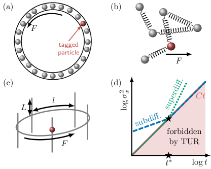
Figure 1: Anomalous diffusion in finite systems. (a) Single file on a ring driven by a force $F$. (b) Tagged-particle diffusion in a harmonic chain. (c) Biased diffusion in a finite (periodic) comb. The experimental observable is the unbounded displacement $x_{t}$ in the direction of the force $F$. (d) The TUR, $\sigma_{x}^{2}(t)\geq Ct$, delivers a threshold time $t^{*}$ that imposes an upper bound on the duration of subdiffusion (dashed blue line) or the earliest possible onset of superdiffusion (dotted green line). The star denotes $K_{\alpha}(t^{*})^{\alpha}=Ct^{*}$ in Eq. (3).

We throughout consider a walker (e.g. a molecular motor) that operates in a (non-equilibrium) steady state [1], which means that the walker’s displacement $x_{t}$ is weakly ergodic. That is, the centralized displacement $x_{t}-vt$ is unbiased with vanishing “ergodicity breaking parameter” [46] (see also [47, 48]), i.e. as long as trajectories are sufficiently long, ensemble- and time-average observables, such as the centralized time averaged mean square displacement (TAMSD) , coincide.

At sufficiently long times where diffusion becomes normal, $\sigma^{2}_{x}(t)\propto t$, the thermodynamic uncertainty relation (TUR) [50, 51] bounds the walker’s variance by

$$\sigma_{x}^{2}(t)\geq\frac{2k_{\rm B}Tv^{2}}{\dot{W}_{\rm ss}}t\equiv Ct,$$ (2)

where $\dot{W}_{\rm ss}$ is the power dissipated by the walker, $k_{\rm B}T$ is the thermal energy, and in the last step we have defined the constant $C$. Eq. (2) is derived by assuming that the underlying (full) system’s dynamics follows a Markovian time evolution. The TUR was originally shown to hold in the long time limit “$t\to\infty$” [50, 51] and later on also at any finite time for a walker’s position evolving from a non-equilibrium steady state [53, *piet16, 55]. Using aspects of information geometry [56, 57, 58] Eq. (2) was recently shown to hold for any initial condition [59]. Subsequent studies have applied Eq. (2) to bound the efficiency of molecular motors [60] and heat engines [61, 62], and extended the TUR to periodically driven systems [63, 64, 65, 66, 67], discrete time processes [68], and open quantum systems [69]. For a broader perspective see [1, 70, 71, 72].

Main result.—We now show how the TUR (2) may be used to obtain a thermodynamic bound on the duration of anomalous diffusion. We first consider subdiffusion ($\alpha<1$) and estimate the largest time $t^{*}$ where Eq. (1) must cease to hold as a result of thermodynamic consistency. Namely, according to (2) subdiffusion in Eq. (1) with constant exponent $\alpha<1$ cannot persist beyond

$$t^{*}\simeq\bigg{(}\frac{K_{\alpha}}{C}\bigg{)}^{1/(1-\alpha)},$$ (3)

see intersecting point in Fig. 1d. Conversely, superdiffusion with an exponent $\alpha>1$ in Eq. (1) cannot emerge before $t^{*}$ (see Fig. 1d). Eq. (3) thus bounds the extent of both sub- and superdiffusion. The bridge between anomalous diffusion and stochastic thermodynamics embodied in Eq. (3) is the main result of this Letter. We note that the bound $t^{*}$ follows directly from the inequality (2) and in general can not be deduced from the long time diffusion behavior (for an explicit counter-example see Supplemental Material (SM) ). In the following we use the three paradigmatic physical models depicted in Fig. 1 to illustrate how to apply the bound (3).

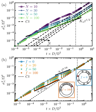
Figure 2: Variance of particle-displacement in a single file on a ring (see Fig. 1a). (a) All $N$ particles are pulled by a Force $F$ (here $F=0$); (b) only the tagged particle is pulled by a force $F\Omega\equiv f\times k_{\rm B}T$ (the inset depicts the effect of $F$) with $N=10$. Symbols represent the centralized TAMSD [49] extracted from a long trajectory $\tau=10^{3}\times D/\Omega^{2}$ for each $N$. The lines are deduced from a modified Jepsen mapping (see SM [73]). Parameters: $D=k_{\rm B}T=\Omega=1$ and $d=0$, i.e., time is measured in units of $D/\Omega^{2}$ and displacements in units of $\Omega=l-Nd$.

Driven single file on a ring.—We first consider a single file of $N$ impenetrable Brownian particles with diameter $d$ and a diffusion coefficient $D$ all dragged with a constant force $F$ described by the Langevin equation $\dot{x}_{i}(t)=\gamma^{-1}F+\xi_{i}(t)$ for $i=1,\ldots N$, where the friction coefficient obeys the fluctuation-dissipation relation $\gamma=k_{\rm B}T/D$ and $\xi_{i}(t)$ represents Gaussian white noise with zero mean and covariance $\langle\xi_{i}(t)\xi_{j}(t^{\prime})\rangle=2D\delta_{ij}\delta(t-t^{\prime})$. The hardcore interaction imposes internal boundary conditions $x_{i}<x_{i+1}+d$ and the confinement to a ring with circumference $l$ (see Fig. 1a) additionally imposes $x_{N}-x_{1}\leq l-d$, i.e., the first particle blocks the passage of the last one. We refer to this setting as “pseudo non-equilibrium” since the transformation to a coordinate system rotating with velocity $v=\gamma^{-1}F$ virtually restores equilibrium dynamics with vanishing current [73]. Nevertheless, the power required to drag the $N$ particles with velocity $v=\gamma^{-1}F$ against the friction force is $\dot{W}^{\rm ss}=N\times Fv$ and Eq. (2) in turn yields $C=2k_{\rm B}T/\gamma N$, a result independent of $F$ (see also [74]).

It is well known that a tracer particle in a dense single-file ($1\ll N<\infty$) exhibits transient subdiffusion according to Eq. (1) with exponent $\alpha\simeq 1/2$ and generalized diffusion constant $K_{\alpha}\simeq 2N^{-1}\Omega\sqrt{D/\pi}$ (see, e.g. [19, 21, 22, 23, 24, 25, 26, 27, 28, 29] and experiments in [30, 31, 32]), where $\Omega\equiv l-Nd$ is the free volume on a ring with circumference $l$. Therefore, the inequality (2) implies that subdiffusion can persist at most until a time $t^{*}=(K_{\alpha}/C)^{1/(1-\alpha)}\simeq\Omega^{2}/(D\pi)$ (see vertical line in Fig. 2a and Eq. (3)).

Thermodynamic consistency limits the extent of subdiffusion to time-scales $t\lesssim t^{*}$. To test the bound in Fig. 2a we determined the centralized TAMSD (see symbols) of a tracer particle from a single trajectory of length $\tau=10^{3}\times(D/\Omega)$ generated by a Brownian dynamics simulation with time increment $dt=10^{-6}\times(D/\Omega)$, and independently deduced $\sigma_{x}^{2}$ also from a mapping inspired by Jepsen [75] (see lines, SM [73] as well as [76, 77]). The results confirm that the TUR sharply bounds the duration of subdiffusion terminating at time $t^{*}$ (see intersection of the TUR-bound and vertical line). If we were to allow particles to overtake the long-time asymptotics would not saturate at the dashed line (see Fig. 10(a-c) in [78]) — in this scenario subdiffusion may terminate before $t^{*}$.

Active single file.—A “genuinely” non-equilibrium steady state is generated by pulling only the tagged particle with a force $F$. The tagged-particle diffusion quantified by $\sigma_{x}^{2}(t)$ is shown in Fig. 2b. Here the non-equilibrium driving force $f\equiv F\times\Omega/k_{\rm B}T$ increases the anomalous exponent from $\alpha\approx 0.58$ to $\alpha\approx 0.69$. Nevertheless, the TUR (dashed line) still tightly bounds the time subdiffusion terminates. Moreover, the onset of subdiffusion is shifted towards shorter times which may be explained as follows. A strongly driven particle “pushes” the non-active particles thereby locally increasing density which in turn shifts the onset of subdiffusion. The effect increases with the strenght of the driving (see inset “$f=100$” in Fig. 2b). This result seemingly contradicts previous findings on active lattice models at high density showing that all even cumulants (incl. the variance) remain unaffected by the driving $f$ [35] (see also [36]). The contradiction is only apparent — single file diffusion for any number of particles in fact corresponds to the low density limit of lattice exclusion models.

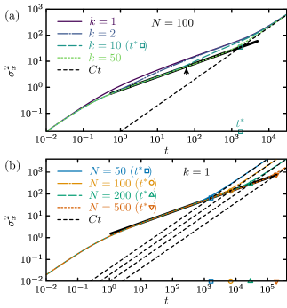
Figure 3: (a) $\sigma_{x}^{2}(t)$ from Eq. (4) for a dragged Gaussian chain with $N=100$ beads, where we tag the $k$th particle ($k=1,2,10,50$). The TUR-bound is shown as the dashed black line. Taking e.g. $k=10$ we find transient subdiffusion $\sigma_{x}^{2}(t)\simeq K_{\alpha}t^{\alpha}$ (solid black line) in the vicinity of $t\sim t_{\rm ref}\equiv 10^{1}$; using Eq. (4) yields the exponent $\alpha\equiv t\partial_{t}\ln\sigma^{2}(t)|_{t=t_{\rm ref}}\approx 0.508$ with $K_{\alpha}\equiv t_{\rm ref}^{-\alpha}\sigma^{2}(t_{\rm ref})$. The rectangle denotes the upper bound on the extent of subdiffusion $t^{*}$ while the vertical arrow highlights the actual time at which the subdiffusive regime for $k=10$ terminates. (b) $\sigma_{x}^{2}(t)$ of the first bead ($k=1$) for increasing $N$. Symbols denote the TUR-bound.

Gaussian chain (Rouse model).—We now consider a harmonic chain with $N$ beads (see Fig. 1b). The equations of motion (for the time being in absence of a pulling force) correspond to [79, 80, 81] $\dot{x}_{k}(t)=-D\sum_{l}H_{kl}x_{l}(t)+\xi_{k}(t)$ where $(\mathbf{H})_{kl}=H_{kl}$ is the Hessian of $U=\sum_{i=2}^{N}(x_{i}-x_{i-1})^{2}/2$. We set $\gamma^{-1}=D$, i.e., $k_{\rm B}T\equiv 1$. The variance of the $k$th bead’s position reads (see e.g. [82])

$$\sigma_{x}^{2}(t)=\frac{2}{N}\left[Dt\!+\!\sum_{p=1}^{N-1}\cos^{2}\!\left(\frac{\pi p(2k-1)}{2N}\right)\frac{1-{\rm e}^{-2D\lambda_{p}t}}{\lambda_{p}}\right]\!,$$ (4)

where $\lambda_{p}=4\sin^{2}(\pi p/2N)$ [79, 80, 81]. The first term in Eq. (4) corresponds to the center-of-mass diffusion.

Suppose now that we drag all particles with a constant force $F$. In this case the force affects only the mean displacements but not the variance [73]. In other words, the left hand side of Eq. (2) is not affected by $F$, whereas the right hand side becomes $C=2D/N$ since $\dot{W}_{\rm ss}=v\times NF$ with $v=\gamma^{-1}F=DF$. By inspecting Eq. (4) directly (note that all terms in Eq. (4) are non-negative) one can verify that the TUR indeed bounds the diffusion of the $k$th particle by $\sigma_{x}^{2}(t)\geq 2Dt/N$ at any time $t$.

In Fig. 3a we inspect the sharpness of the bound. For example, tagging the $10$th bead in a polymer with $N=100$ we observe subdiffusion with an exponent $\alpha\approx 0.508$ (see thick black line) that terminates at $t<t^{*}$ (see vertical arrow), i.e. faster than predicted by the TUR (see green rectangle). Interestingly, the scaling of $\sigma_{x}^{2}(t)$ at this point does not become normal with $\alpha=1$ but instead turns to a second, slightly larger anomalous exponent. Normal diffusion is in fact observed at much longer times. This example highlights that subdiffusion with an (initial) exponent $\alpha$ cannot extend beyond $t^{*}$. However, this does not imply that $t^{*}$ necessarily corresponds to the onset of normal diffusion. Conversely, if we tag the first particle of the chain (see Fig. 3b) the TUR bounds the overall duration of subdiffusion quite tightly. According to Eq. (3) the longest time subdiffusion can persist increases with $N$ as $t^{*}\propto C^{-2}\propto N^{2}$ (see symbols in Fig. 3b as well as [17]).

Superdiffusion in the active comb model.—So far we have discussed only systems exhibiting subdiffusion. To address superdiffusion we consider the “active comb model” depicted in Fig. 1c corresponding to diffusion on a ring with side-branches with a finite length $L$ oriented perpendicularly to the ring at positions separated by $l$. Within the ring (but not in the side-branches) the particle is dragged with a constant force $F$. For simplicity we assume the diffusion constant, $D$, to be the same in the ring and along the side-branches. The probability density and flux are assumed to be continuous at the intersecting nodes such that the steady state probability to find the particle in the ring (i.e. in a “mobile state”) corresponds to $\phi_{m}=l/(l+2L)$ yielding a mean drift velocity $v=\beta DF\phi_{m}$. Using $\dot{W}_{\rm ss}=Fv$ alongside the TUR (Eq. (2)) we immediately obtain $\sigma_{x}^{2}(t)\geq 2\phi_{m}Dt$. It is known that infinite side-branches “$L=\infty$” in the passive comb model (i.e. $F=0$) break ergodicity. That is, a non-equilibrium steady state ceases to exist and subdiffusion with exponent $\alpha=1/2$ persists for any fixed initial condition and time $t$ (e.g., see [40, 41, 42]). Conversely, a bias $F\neq 0$ in a finite comb ($L<\infty$) was found, quite counterintuitively, to enhance the long time diffusion [39], which leads to transient superdiffusion as discussed below.

The particle’s position along the ring does not change while it is in a side-branch. Therefore, only the (random) “occupation time in the mobile phase” [83, 84], $\tau_{m}(t)\leq t$, is relevant. Its fraction is referred to as the “empirical density” [85, 84] since $\langle\tau_{m}(t)\rangle=\phi_{m}t$.

The particle drifts with velocity $\beta DF$ and diffuses with diffusion constant $D$ during the time $\tau_{m}(t)$ it spends in the ring. This implies a displacement distributed according to $x_{t}\sim\beta DF\tau_{m}(t)+\sqrt{2D\tau_{m}(t)}\mathcal{N}$, where $\mathcal{N}$ is a standard normal random number, which eventually leads to (for an alternative derivation see [39])

$$\sigma_{x}^{2}(t)=2D\phi_{m}t+(\beta DF)^{2}\sigma_{\tau}^{2}(t),$$ (5)

where we used $\langle\mathcal{N}^{2}\rangle=1$, $\langle\mathcal{N}\rangle=0$, $\langle\tau_{m}(t)\rangle=\phi_{m}t$ and defined $\sigma_{\tau}^{2}(t)\equiv\langle\tau_{m}(t)^{2}\rangle-\langle\tau_{m}(t)\rangle^{2}$. To deduce $\sigma_{\tau}^{2}(t)$ we translated the equation of motion into a Markov jump system according to [86] and used a spectral expansion [84] which alongside Eq. (5) yields $\sigma_{x}^{2}(t)$. The result for $l=3$ and $L=10$ [73] is shown in Fig. 4. The thick lines denote power laws with a “maximal exponent” $\alpha=\max_{t}t\partial_{t}\ln\sigma_{x}^{2}(t)$ (see inset for the respective values). At equilibrium ($F=0$) the diffusion is normal at all times. The presence of a force causes transient superdiffusion with an exponent approaching the ballistic regime $\alpha\approx 2$ upon increasing $F$. Note that here the TUR bounds the time of initiation of superdiffusion (see symbols) and not the termination.

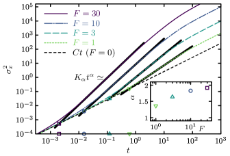
Figure 4: $\sigma_{x}^{2}$ in the driven comb model (see Fig. 1d). We consider various driving forces $F$ and side-branches with length $L=10$ separated by a distance $l=3$ yielding a steady state probability in the ring $\phi_{m}=l/(l+2L)=3/23\approx 0.13$ with $D=\beta=1$. The force-free case $F=0$ coincides with the bound $Ct$ in Eq. (2). The thick lines correspond to $K_{\alpha}t^{\alpha}$ with the “maximal exponent” $\alpha\equiv\max_{t}t\partial_{t}\ln\sigma_{x}^{2}(t)$ depicted in the inset. Symbols denote the time $t^{*}$ in Eq. (3) where $K_{\alpha}t^{\alpha}$ and $Ct$ intersect. Long times $t\to\infty$ and strong driving $\beta Fl\gg 1$ yield $\sigma_{x}^{2}\simeq 2D\phi_{m}t+(\beta Fl)^{2}(1-\phi_{m})^{3}Dt/6$.

To explain this we must understand when $\sigma_{\tau}^{2}(t)$ increases non-linearly with $t$. One can show that for sufficiently small times $t\to 0$ the particle is found with high probability either only in the ring or only in one of the side-branches which yields a vanishing variance $\sigma_{\tau}^{2}(t)=\mathcal{O}(t)$. Conversely, we have recently found [84] that the dispersion of the fraction of occupation time at long times, $\mathcal{D}\equiv\lim_{t\to\infty}\sigma_{\tau}^{2}(t)/t$, is entirely encoded in the (steady state) joint return probability, $P(m,t,m)$, i.e. the probability to be in the mobile region $m$ initially and again at time $t$

$$\mathcal{D} =2\int_{0}^{\infty}[P(m,t,m)-\phi_{m}^{2}]\mathrm{d}t$$

$$=\frac{4lL^{2}[(\beta F)^{2}lL+3\beta Fl\coth(\beta Fl/2)-6]}{3D(\beta F)^{2}(l+2L)^{3}},$$ (6)

where the first line is shown in [84], and the second line is derived in [73] (a similar result is found in [39]). At strong driving $\beta Fl\gg 1$ we find $\mathcal{D}\simeq l^{2}(1-\phi_{m})^{3}/6$ which interestingly enhances diffusion $\propto(\beta Fl)^{2}(1-\phi_{m})^{3}$ by a magnitude that increases with the likelihood to reside immobile. Superdiffusion thus arises from an interplay between effectively “ballistic” transport in the ring and pausing in the side-branches, and becomes pronounced at strong driving $\beta Fl\gg 1$ and in the presence of long side-branches $L\gg l$, yielding $1-\phi_{m}\approx 1$. A similar effect gives rise to the so-called Taylor dispersion [87] that occurs in diffusion in a flow field [88, 89, 90].

Conclusion.—We established a bridge between anomalous diffusion and the TUR by explaining how the latter can be utilized to (sharply) bound the temporal extent of anomalous diffusion in finite systems driven out of equilibrium. We used the TUR to demonstrate that a non-equilibrium driving may in fact be required for anomalous dynamics to occur such as e.g. in the comb model. We have shown that the TUR can also bound the duration of anomalous diffusion in systems obeying detailed balance if we are able to construct a fictitious non-equilibrium system with the same dynamics, which we demonstrated by means of the passive and driven single file and the Rouse polymer. In this context it will be useful to deepen the connection between the TUR [91] and anomalous transport [92, 93] close to equilibrium, growing interfaces [94, 95], and to bound subdiffusion in flexible gel networks [96].

Finally, we point out that the TUR (Eq. (2)) and therefore our results apply to overdamped systems (i.e., when momenta relax “instantaneously”). If we include momenta or consider the presence of magnetic fields the TUR requires modifications [97, 98]. Such extensions will allow to bound the extent of anomalous diffusion in underdamped systems [99, 100, 101, 102, 103]. Finally, the recent generalization of the TUR [59, 67, 104] will allow applying the TUR to anomalous diffusion and anomalous displacements arising from non-stationary and non-ergodic infinite systems [35].

Supplemental Material

In this Supplemental material we first clarify why the long time diffusion does not suffice to bound the extent of anomalous subdiffusion (see Sec. .1). In Sec. .2 we show that the thermodynamic uncertainty relation can also be applied to interacting many particle systems at equilibrium if one can construct/identify a “pseudo non-equilibrium state”. We explain the mapping motivated by Jepsen that we used to analyze the single-file system (lines in Fig. 2 in the main text) in Sec. .3. In Sec..4 we derive the second line in Eq. (6) in the main text and provide details about the numerical implementation of the comb-model (see Fig. 4 in the main text).

.1 Long time diffusion does not bound the extent of anomalous diffusion

In the limit of ergodically long times the variance will grow linearly in time with a diffusion coefficient $D_{\infty}$ which follows from $\sigma_{x}^{2}(t)/(2t)\to D_{\infty}$ or $\sigma_{x}^{2}(t)\simeq 2D_{\infty}t$ in the limit $t\to\infty$. Note that the limit $\sigma_{x}^{2}(t)/(2t)\to D_{\infty}$ does not exclude the possibility of approaching $D_{\infty}t$ from below. Therefore, knowing $D_{\infty}$ alone cannot suffice to bound the extent of subdiffusion. To illustrate this we consider an approach of the long time diffusion from below as shown in Fig. S5. From the long time asymptotics we would “erroneously” underestimate the latest end of subdiffusion with a constant exponent $\alpha<1$ (see triangle). The inequality “$\geq$” involving the thermodynamic uncertainty relation (TUR), $\sigma_{x}^{2}(t)\geq Ct$, prevents any approach to normal diffusion to intermediately cross the red line. Thus $t^{*}$ is always guaranteed to be the latest time when subdiffusion with a constant anomalous exponent must end.

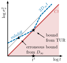
Figure S5: Knowing the long time diffusion $D_{\infty}$ alone does not suffice to bound the extent of subdiffusion.

.2 Uncertainty relation at equilibrium – pseudo non-equilibrium

In this section we explain how the thermodynamic uncertainty relation obeyed by non-equilibrium systems, under given conditions can also be applied to interacting colloidal particles at equilibrium. To this end we consider translationally invariant systems that are at equilibrium with zero drift velocity $v=0$. Adding a drift $\alpha=vt$ to all coordinates transforms to system to what we call “pseudo non-equilibrium”. In the following two paragraphs we explain that the drifting pseudo non-equilibrium and the corresponding non-drifting equilibrium system display the same variance $\sigma_{x}^{2}(t)\big{|}_{v=0}=\sigma_{x}^{2}(t)\big{|}_{v\neq 0}$.

Let us first explain this idea mathematically. Consider a random variable $X$ and a shifted random variable $Y+\alpha$, where $\alpha$ is some constant. The variance is known to be invariant with respect to such a constant bias, i.e. $\operatorname{Var}(Y)=\operatorname{Var}(X+\alpha)=\operatorname{Var}(X)$. In the following we prove this mathematical property in the context of physically interacting particles.

Consider $N$ colloidal particles interacting via a pairwise additive interaction potential $U(\boldsymbol{x})=\sum_{i<j}U_{ij}(x_{i}-x_{j})$, where $\boldsymbol{x}=(x_{1},\ldots,x_{N})=\boldsymbol{x}(t)$ is a vector with all particle positions at time $t$. At equilibrium the colloidal particles obey the set of coupled Langevin equations

$$\dot{x}_{i}(t)=-\gamma^{-1}\partial_{x_{i}}U(\boldsymbol{x})+\xi_{i}(t),$$ (S7)

where $\xi_{t}$ is Gaussian white noise with zero mean and covariance $\langle\xi_{i}(t)\xi_{j}(t^{\prime})\rangle=2\delta_{ij}\delta(t-t^{\prime})$. We now add a drift to all particle positions such that $y_{i}\equiv x_{i}(t)+vt$ (for all $i$). The constant velocity may arise from a drifting coordinate system with constant velocity $v$. In this case the system is only fictitiously driven out of equilibrium [105] to which we refer as “pseudo non-equilibrium”. Note that the same “pseudo non-equilibrium” state may also be generated by a “real” physical force $F$, i.e. $v=\gamma^{-1}F$. In both cases the drifted colloidal particles satisfy the Langevin equations

$$\dot{y}_{i}(t)=v-\gamma^{-1}\partial_{x_{i}}U(\boldsymbol{x})+\xi_{t}=\gamma^{-1}F-\gamma^{-1}\partial_{y_{i}}U(\boldsymbol{y})+\xi_{t},$$ (S8)

where in the last step we defined $\gamma^{-1}F\equiv v$ and used $U_{ij}(y_{i}-y_{j})=U_{ij}(x_{i}+vt-x_{j}-vt)=U_{ij}(x_{i}-x_{j})$. Eq. (S8) establishes that $y_{i}\equiv x_{i}(t)+\gamma^{-1}Ft$ connects equilibrium dynamics $\{x_{i}(t)\}$ to a fictitiously dragged system $\{y_{i}(t)\}$. For any fixed $\tau$ the displacement after time $t$ using $\delta x_{i}(t)\equiv x_{i}(t+\tau)-x_{i}(\tau)$, becomes $\delta y_{i}(t)\equiv y_{i}(t+\tau)-y_{i}(\tau)=\delta x_{i}(t)+\gamma^{-1}Ft$, which yields the variance

$$\sigma_{y}^{2}(t) \equiv\langle\delta y_{i}(t)^{2}\rangle-\langle\delta y_{i}(t)\rangle^{2}$$

$$=\langle[\delta x_{i}(t)+\gamma^{-1}Ft]^{2}\rangle-[\langle\delta x_{i}(t)\rangle+\gamma^{-1}Ft]^{2}$$

$$=\langle\delta x_{i}(t)^{2}\rangle-\langle\delta x_{i}(t)\rangle^{2}=\sigma_{x}^{2}(t).$$ (S9)

Thus the driven ($F\neq 0$) and equilibrium ($F=0$) system have exactly the same variance.

In the pseudo non-equilibrium state (S8) the dissipation rate becomes $\dot{W}_{\rm ss}=NFv=N\gamma v^{2}$. Using the fluctuation dissipation relation $\gamma=k_{\rm B}T/D$ yields $\dot{W}_{\rm ss}=Nk_{\rm B}T/D$ which with Eq. (2) in the main text yields $C=2D/N$ – a result that is independent of the force. This result in conjunction with the preservation of variance, Eq. (S9), in turn yields

$$\sigma_{x}^{2}(t)\big{|}_{F=0}=\underbrace{\sigma_{y}^{2}(t)\big{|}_{F\neq 0}\geq Ct\big{|}_{F\neq 0}}_{\text{TUR}}=Ct\big{|}_{F=0},$$ (S10)

which completes the proof that the TUR may be applied to equilibrium systems for which we are able to construct a pseudo non-equilibrium that displays the same variance.

We employed the TUR according to Eq. (S10) for the derivation of the results depicted in Fig. 2a (single-file) and Fig. 3 (Gaussian chain). The comb model from Fig. 1c in the main text is not translation invariant due to the side-branches with length $L$, which is why the the result depicted in Fig. 4 in the main text cannot be studied in this manner. Moreover, the driving force in the active single file (Fig. 2b in the main text) affects the interaction between particles (see insets). Thus Eq. (S10) is bound to hold only if both the system is translational invariant and the same biasing force is applied to all particles. In the following subsection we discuss a translational invariant system – the single file.

.3 Single file

Jepsen mapping in the single file. For simplicity we set the length of the ring to $l=1$ and diameter $d=0$ such that the particle position $\boldsymbol{\theta}=(\theta_{1},\ldots,\theta_{N})$ will satisfy

$$\theta_{1}(t)\leq\theta_{2}(t)\leq\ldots\leq\theta_{N}(t)\quad\text{and}\quad\theta_{N}(t)-\theta_{1}(t)\leq 1.$$ (S11)

Without loss of generality we keep $d=0$ and $l=1$. Note that the problem of having particles with finite diameter $d>0$ moving on ring with circumference $l$ can be restored easily via the mapping $\theta_{i}(t)\to(l-Nd)\theta_{i}(t)+(i-1)d$.

The first expression in Eq. (S11) means that the particles cannot penetrate each other such that the order is preserved, and the last condition is due to the ring-like structure and means that the last particle – the $N$th one – cannot advance the first particle by more than one circumference $l=1$. Let us now consider the method developed by Jepsen [75] (e.g., see also Refs. [76, 77, 106]), which allows us to map the system of interacting particles through Eq. (S11) onto a system of non-interacting particles $\tilde{\boldsymbol{\theta}}$ that may violate Eq. (S11). Jepsen [75] derived a mapping which restores the first expression in Eq. (S11) by permuting the particles positions “$\operatorname{sort}(\cdots)$” into increasing order such that $\operatorname{sort}(\tilde{\boldsymbol{\theta}})$ satisfies the first condition in (S11), i.e.,

$$\operatorname{sort}[\tilde{\boldsymbol{\theta}}]_{1}\leq\operatorname{sort}[\tilde{\boldsymbol{\theta}}]_{2}\leq\ldots\leq\operatorname{sort}[\tilde{\boldsymbol{\theta}}]_{N}.$$ (S12)

To also restore the second condition we need to go beyond Ref. [75] and find a map $\mathcal{M}(\tilde{\boldsymbol{\theta}})=\boldsymbol{\theta}$, which also restores the periodic boundary condition in (S11). That is, we need to find the mapping $\mathcal{M}$ that fully restores Eq. (S11). Introducing the element-wise floor function $\lfloor\cdot\rfloor$, adopting the sorting function (S12), defining the mean value of a vector $\boldsymbol{y}$ through $\overline{\boldsymbol{y}}\equiv N^{-1}\sum_{i=1}^{N}y_{i}=\overline{\operatorname{sort}(\boldsymbol{y})}$, the desired mapping $\mathcal{M}$ is given by

$$\begin{pmatrix}\theta_{1}\\ \vdots\\ \theta_{N-\nu}\\ \theta_{N-\nu+1}\\ \vdots\\ \theta_{N}\end{pmatrix}=\mathcal{M}(\tilde{\boldsymbol{\theta}})=\begin{pmatrix}\operatorname{sort}(\tilde{\boldsymbol{\theta}}-\lfloor\tilde{\boldsymbol{\theta}}\rfloor)_{\nu+1}+\vartheta\\ \vdots\\ \operatorname{sort}(\tilde{\boldsymbol{\theta}}-\lfloor\tilde{\boldsymbol{\theta}}\rfloor)_{N}+\vartheta\\ \operatorname{sort}(\tilde{\boldsymbol{\theta}}-\lfloor\tilde{\boldsymbol{\theta}}\rfloor)_{1}+\vartheta+1\\ \vdots\\ \operatorname{sort}(\tilde{\boldsymbol{\theta}}-\lfloor\tilde{\boldsymbol{\theta}}\rfloor)_{\nu}+\vartheta+1\end{pmatrix},$$ (S13)

where

$$\vartheta\equiv\lfloor\overline{\lfloor\tilde{\boldsymbol{\theta}}\rfloor}\rfloor\quad\text{and}\quad\nu=N\overline{\lfloor\tilde{\boldsymbol{\theta}}\rfloor}-N\vartheta.$$ (S14)

The mapping (S13) can be shown to restore Eq. (S11) entirely and to preserve the total displacement $\sum_{i=1}^{N}\theta_{i}(t)=\sum_{i=1}^{N}\tilde{\theta}_{i}(t)$. Note that the variable $\vartheta$ (and $\vartheta+1$) in Eq. (S13) counts the number complete revolutions in the ring $\vartheta+\nu$.

Without loss of generality we tag particle 1 such that the displacement of the tagged particle becomes $x_{t}=\theta_{1}(t)-\theta_{1}(0)$. Note that a particle with non-zero diameter $d$ and ring with length $l$ (incl. $l\neq 1$) can be accounted for by $x_{t}=\Omega[\theta_{1}(t)-\theta_{1}(0)]$, where $\Omega=l-Nd$.

Numerical evaluation of the variance $\sigma_{x}^{2}(t)$. We determine $\sigma_{x}^{2}(t)$ at any distant time $t$ by directly evaluating $10^{4}$ realizations of positions $x_{t}$ at time $t$. Each position $x_{t}$ is generated as follows (we set $d=0$, $\Omega=l=1$).

• Distribute all particles $i=1,\ldots,N$ uniformly on the scaled ring via $u_{i}\sim\operatorname{uniform}[0,1]$ and sort them $\tilde{\theta}_{i}(t)=\operatorname{sort}(\boldsymbol{u})_{i}$.

• Generate $N$ standard normal Gaussian random variables $Z_{1},\ldots,Z_{N}$ and propagate the scaled coordinate $\tilde{\theta}_{i}(t)=\tilde{\theta}_{i}(0)+\Omega^{-1}[\gamma^{-1}Ft+\sqrt{2Dt}\cdot Z_{i}]$ for $i=1,\ldots,N$

• Restore the order of particles by backtracking all collisions, which is attained by evaluating $\boldsymbol{\theta}(t)=\mathcal{M}(\tilde{\boldsymbol{\theta}}(t))$ from Eqs. (S13) and (S14). Note that $\boldsymbol{\theta}(0)=\mathcal{M}(\tilde{\boldsymbol{\theta}}(0))=\tilde{\boldsymbol{\theta}}(0)$.

• One realization of the displacement of the tagged particle is obtained from $x_{t}=\Omega[\theta_{1}(t)-\theta_{1}(0)]$. Here $\Omega=1$.

A realization of the displacement $x_{t}$ after any time $t$ is obtained according to steps (i)-(iv). For each time $t$ in Fig. 2a in the Letter we evaluated (see lines) $10^{4}$ displacements $x_{t}$ and deduced their corresponding variance. In contrast to the Brownian Dynamics simulation (see symbols) the steps (i)-(iv) avoid any intermediate time step in the simulation. Note that this efficient mapping can only be used when all particles are dragged by the same force (see Fig. 2a in the main text). As soon as only one particle is dragged as depicted in Fig. 2b in the main text the method developed by Jepsen cannot be employed.

.4 Comb model

.4.1 Comb model dynamics

As explained in the main text it suffices to merely focus on the stochastic time $\tau_{m}(t)$ spend in the “mobile” ring region. Since the comb is assumed to be periodic we merely focus on one period from one pair of side-branches to the next. We call $P_{0}(x,t)$ the probability density to find the particle in the “mobile” ring at distance $x$ along the force $F$ from the “previous” side branch. We further denote the probability density within any of the two side-branches to be at time $t$ the distance $y$ away from the “mobile” ring by $P_{y}(0,t)$. The probability density $P_{y}(x,t)$ satisfies $\int_{0}^{L}P_{y}(0,t)\mathrm{d}y+\int_{0}^{l}P_{0}(x,t)\mathrm{d}y=1$. The Fokker-Planck equation then reads

$$\partial_{t}P_{y}(0,t) =D\partial_{y}^{2}P_{y}(0,t),$$ (S15)

$$\partial_{t}P_{0}(x,t) =-D[\beta F\partial_{x}-\partial_{x}^{2}]P_{0}(x,t),$$

where $0\leq x\leq l$ and $0\leq y\leq L$, along with the boundary condition $P_{0}(0_{+},t)=P_{0}(l-0_{+},t)=P_{0_{+}}(0,t)/2$ (division by 2 accounts for two side-branches) and conservation of probability $P_{0}(0_{+},t)+\partial_{x}P_{0}(0_{+},t)=\partial_{x}P_{0}(l-0_{+},t)$ as well as $\partial_{y}P_{L}(0,t)=0$. Eq. (S15) corresponds to a diffusion on a piece-wise one dimensional graph [107]. The stationary state probability density becomes $P_{0}(x,\infty)=1/(2L+l)$ and $P_{y}(0,\infty)=2/(2L+l)$. The mean occupation time in the mobile state becomes $\langle\tau_{m}(t)\rangle=t\int\mathrm{d}xP_{0}(x,\infty)=lt/(2L+l)=\phi_{m}t$, where $\phi_{m}\equiv l/(2L+l)$. In the remainder of this section we determine the variance of the occupation time $\sigma_{\tau}^{2}(t)=\langle\tau_{m}(t)^{2}\rangle-\langle\tau_{m}(t)\rangle^{2}$.

.4.2 Numerical solution of the driven comb model

To solve the Fokker-Planck equation numerically according to Ref. [86] we translate the partial differential equation into a master equation, i.e., a random walk on a discrete grid with equidistant spacing $\delta$ such that the ring states $z=0,1,\ldots,N_{1}$ ($N_{1}=l/\delta$) correspond to positions $x=0,\delta,\ldots,\delta N_{1}$, while states belonging to the side-branches separated by $\delta$ are $z=0,(N_{1}+1),(N_{1}+2),\ldots,(N_{1}+N_{2})$ and correspond to the positions $y=0,\delta,\ldots,N_{2}\delta$ ($N_{2}=L/\delta$). For convenience we assume that both $l/\delta$ and $L/\delta$ are integer valued. The transition rates within the “ring states” $z\in\{0,1,\ldots N_{1}\}$ are given by

$$R_{z\to z+1} =\frac{D{\rm e}^{\beta DF\delta/2}}{\delta^{2}},\quad\text{for $0\leq z\leq N_{1}-1$}$$ (S16)

$$R_{N_{1}\to 0} =\frac{D{\rm e}^{\beta DF\delta/2}}{\delta^{2}},\quad R_{0\to N_{1}}=\frac{D{\rm e}^{-\beta DF\delta/2}}{\delta^{2}},$$

$$R_{z\to z-1} =\frac{D{\rm e}^{-\beta DF\delta/2}}{\delta^{2}},\quad\text{for $1\leq z\leq N_{1}$},$$

and the transition rates in the states belonging to side branches $z\in\{0,N_{1}+1,N_{1}+2,\ldots N_{2}\}$ are given by

$$R_{z\to z+1} =R_{z+1\to z}=\frac{D}{\delta^{2}},\quad\text{for $N_{1}+1\leq z\leq N_{2}-1$},$$ (S17)

$$R_{0\to N_{1}+1}/2 =R_{N_{1}+1\to 0}=\frac{D}{\delta^{2}},$$

while all the remaining rates that are not listed in Eqs. (S16) and (S17) are set to zero. Note that the division by 2 in the second line of Eq. (S17) accounts for the degeneracy due to having two side-branches. The generator of the master equation reads

$$\mathcal{L}_{zz^{\prime}}=\begin{cases}R_{z^{\prime}\to z},&\text{if $z\neq z^{\prime}$},\\ -R_{z},&\text{if $z=z^{\prime}$},\end{cases}$$ (S18)

where $R_{z}\equiv\sum_{z^{\prime}\neq z}R_{z\to z^{\prime}}$ and $z\in\{0,1,\ldots,N_{1}+N_{2}\}$. We numerically perform a complex eigendecomposition of the generator $\mathcal{L}$

$$\mathcal{L}=-\sum_{i=0}^{N_{1}+N_{2}-1}\lambda_{i}|\psi_{i}^{\rm R}\rangle\langle\psi_{i}^{\rm L}|,$$ (S19)

where $\lambda_{k}$ is the $k$th eigenvalue and $\psi_{i}^{\rm L}$ (or $\psi_{i}^{\rm L}$) are the corresponding left (or right) eigenvectors which according to Eq. (S19) are normalized $\langle\psi_{i}^{\rm L}|\psi_{j}^{\rm R}\rangle=\delta_{ij}$; note that $\lambda_{0}=0$. According to Eq. (52) in Ref. [84] the variance of the occupation time in all the ring states becomes

$$\sigma_{\tau}^{2}(t)=2t\sum_{i=1}^{N_{1}+N_{2}-1}\frac{V_{0i}V_{i0}}{\lambda_{i}^{\dagger}}\bigg{[}1-\frac{1-{\rm e}^{\lambda_{i}^{\dagger}t}}{\lambda_{i}^{\dagger}t}\bigg{]},$$ (S20)

where $V_{ij}=\sum_{k=0}^{N_{1}}\langle\psi_{i}^{\rm L}|k\rangle\langle k|\psi_{j}^{\rm R}\rangle$ and $\lambda_{i}^{\dagger}$ is the complex conjugate of the eigenvalue $\lambda_{i}$ (see also Ref. [108]). The lines in Fig. 4 in the main text are obtained from Eq. (S20) with $D=\beta=1,l=3,L=10$, and $\delta=0.01$, i.e., $N_{1}=300$ and $N_{2}=1000$.

.4.3 Analytical long-time asymptotics

We now provide the background and intuition about Eq. (6) that addresses the long time limit and is adopted from Eq. (61) in Ref. [84]. The long time dispersion is characterized by the first term in Eq. (S20), i.e.,

$$\mathcal{D} =\lim_{t\to\infty}\frac{\sigma_{\tau}^{2}(t)}{t}=2\sum_{i=1}^{N_{1}+N_{2}-1}\frac{V_{0i}V_{i0}}{\lambda_{i}^{\dagger}}$$

$$=2\int_{0}^{\infty}\mathrm{d}t\Bigg{[}\sum_{i=0}^{N_{1}+N_{2}-1}V_{0i}V_{i0}{\rm e}^{-\lambda_{i}^{\dagger}t}-V_{00}V_{00}\Bigg{]},$$ (S21)

where in the second line we used $\int_{0}^{\infty}{\rm e}^{-\lambda t}=1/\lambda$ and $\lambda_{0}=0$. Identifying $V_{00}=\phi_{m}$ and $\sum_{i=0}^{N_{1}+N_{2}-1}V_{0i}V_{i0}{\rm e}^{-\lambda_{i}^{\dagger}t}=P(m,t|m)\phi_{m}=P(m,t,m)$ yields the first line in Eq. (6) in the main text. Note the exact solution corresponds to the limit $N_{1},N_{2}\to\infty$.

To obtain the second line of Eq. (6) in the main text, it proves convenient to Laplace transform the time domain $t\to s$ such that any function $f(t)$ becomes $\tilde{f}(s)=\int_{0}^{\infty}{\rm e}^{-st}f(t)\mathrm{d}t$. In this case the Fokker-Planck equation can be conveniently solved analytically. Moreover, the long time dispersion is then obtained from

$$\mathcal{D} =2\int_{0}^{\infty}\mathrm{d}t[P(m,t,m)-\phi_{m}^{2}]$$

$$=2\lim_{s\to 0}\Big{[}\tilde{P}(m,s,m)-\frac{\phi_{m}^{2}}{s}\Big{]}.$$ (S22)

Thus it suffices to determine the Laplace transform, $\tilde{P}(m,s,m)$, of the joint probability density $P(m,t,m)$ to be in the mobile state and return to it again at time $t$.

We define the propagator as $P_{y}(x,t|x_{0})=P_{y}(x,t)$ with the initial condition $P_{y}(x,0)=\delta(x-x_{0})$ and $P_{y}(0,0)=0$ (we start in the mobile ring). The return probability is obtained from integrating the propagator over the mobile region $P(m,t,m)=\int_{0}^{l}\mathrm{d}x\int_{0}^{l}\mathrm{d}x_{0}P_{0}(x,t|x_{0})\phi_{m}/l$, where $\phi_{m}/l=P_{0}(x_{0},\infty)$ is the stationary probability density within the ring. The propagator satisfies the Fokker-Planck equation (S15), which after Laplace transformation and setting $D\equiv\beta\equiv 1$ becomes

$$\tilde{P}_{0}(x,s|x_{0}) =\delta(x-x_{0})$$ (S23)

$$[-\partial_{y}^{2}+s]\tilde{P}_{y}(0,s|x_{0})=0$$

where $0\leq y\leq L$ and $0\leq x\leq l$ and with boundary conditions translating into $\tilde{P}_{0}(0_{+},s|x_{0})=\tilde{P}_{0}(l-0_{+},s|x_{0})=2\tilde{P}_{0_{+}}(0,s|x_{0})$ and $\partial_{x}\tilde{P}_{0}(0_{+},s|x_{0})+\partial_{y}\tilde{P}_{0_{+}}(0,s|x_{0})=\partial_{x}\tilde{P}_{0}(l-0_{+},s|x_{0})$ as well as $\partial_{y}\tilde{P}_{L}(0,s|x_{0})=0$.

The solution of Eq. (S23) for any $s$ can be obtained straightforwardly using the ansatz $\tilde{P}_{y}(0,s|x_{0})=\psi_{0}(y)=a_{0}\cosh[\sqrt{s}(L-y)]$, which solves the second line of Eq. (S23) with boundary condition $\partial_{y}\tilde{P}_{L}(0,s|x_{0})=\psi_{0}^{\prime}(L)=0$. Moreover, the first line of Eq. (S23) is solved by

$$\tilde{P}_{0}(x,s|x_{0})=\begin{cases}\psi_{1}(x)&\text{if $x\leq x_{0}$},\\ \psi_{2}(x)&\text{if $x>x_{0}$},\end{cases}$$ (S24)

where we use $\psi_{i}(x)=a^{+}_{i}{\rm e}^{\mu_{+}x}+a^{-}_{i}{\rm e}^{\mu_{-}x}$ for $i=1,2$ with $\mu_{\pm}=F/2\pm\sqrt{F^{2}/4+s}$. Note that the five parameters $a_{0},a^{+}_{1},a^{-}_{1},a^{+}_{2},a^{-}_{2}$ are determined from the boundary conditions which read

$$\psi_{1}(0) =\psi_{2}(l)=\psi_{0}(0)/2, \psi_{1}(x_{0}) =\psi_{2}(x_{0}),$$ (S25)

$$\psi_{2}^{\prime}(l) =\psi_{0}^{\prime}(0)+\psi_{1}^{\prime}(0) \psi_{1}^{\prime}(x_{0})-\psi_{2}^{\prime}(x_{0}) =1,$$

where the second condition of the last line follows from the inhomogeneity caused by “$\delta(x-x_{0})$” in Eq. (S23). The results of $a_{0},a^{+}_{1},a^{-}_{1},a^{+}_{2},a^{-}_{2}$ are too lengthy to be displayed and it turned out that they do not need to be precisely known.

We first perform the integral over the mobile ring “$x$”

$$\tilde{P}(m,s|x_{0})\equiv\int_{0}^{l}\mathrm{d}x\tilde{P}_{0}(x,s|x_{0})\\ =\frac{1}{s}-\int_{0}^{L}\mathrm{d}y\tilde{P}_{y}(0,s|x_{0})=\frac{1}{s}-a_{0}\frac{\sinh(\sqrt{s}L)}{\sqrt{s}},$$ (S26)

where in the first step in the second line we used that the probability is conserved and a constant “1” after Laplace transform in time becomes “$1/s$”, while in the very last step we identified the parameter $a_{0}$, which does not depend on $x$ whereas it does depend on $x_{0}$ and $s$. The joint return probability is obtained from Eq. (S26) via

$$\tilde{P}(m,s;m) =\int_{0}^{l}\mathrm{d}x_{0}\tilde{P}(m,s|x_{0})\frac{1}{2L+l}$$

$$=\frac{\phi_{m}}{s}-\frac{\sinh(\sqrt{s}L)}{\sqrt{s}(2L+l)}\int_{0}^{l}a_{0}\mathrm{d}x_{0}$$ (S27)

Inserting $a_{0}$, which solves the system of equations Eq. (S25), into Eq. (S27) and using Eq. (S22) finally yields

$$\mathcal{D} =2\lim_{s\to 0}\Bigg{[}\frac{\phi_{m}(1-\phi_{m})}{s}+\frac{\sinh(\sqrt{s}L)}{\sqrt{s}(2L+l)}\int_{0}^{l}a_{0}\mathrm{d}x_{0}\Bigg{]}$$

$$=\frac{4lL^{2}(F^{2}lL+3Fl\coth(Fl/2)-6)}{3F^{2}(l+2L)^{3}}.$$ (S28)

In the last step we have used the computer algebra program wolfram mathematica which allowed us to conveniently carry out these straightforward albeit tedious calculations. This final step in (S28) finally proves Eq. (6) in the main text. Note we here used $\beta=D=1$. To restore the units we use $\mathcal{D}\to\mathcal{D}/D$ and $F\to\beta F$.