Lattice QCD equation of state at finite chemical potential from an alternative expansion scheme

Abstract

Taylor expansion of the equation of state of QCD suffers from shortcomings at chemical potentials $\mu_{B}\geq(2-2.5)T$. First, one faces difficulties inherent in performing such an expansion with a limited number of coefficients; second, higher order coefficients determined from lattice calculations suffer from a poor signal-to-noise ratio. In this work, we present a novel scheme for extrapolating the equation of state of QCD to finite, real chemical potential that can extend its reach further than previous methods. We present continuum extrapolated lattice results for the new expansion coefficients and show the thermodynamic observables up to $\mu_{B}/T\leq 3.5$.

I Introduction

The phase diagram of Quantum Chromodynamics (QCD) is an open field of investigation, which is currently at the center of intense efforts from the theoretical and experimental communities alike. At vanishing baryon density, the transition between confined and deconfined matter is known to be an analytic crossover [1]. This knowledge was gained through lattice simulations, which represent a systematically improvable method to solve equilibrium QCD. Although at finite baryon density lattice QCD faces a sign problem, numerous results have been published for moderate chemical potentials in recent years [2, 3]. New techniques that allow for direct simulations at finite chemical potential in the presence of a sign problem are the subject of intense investigation. Promising results are available from Lefschetz thimbles [4, 5, 6], the Complex Langevin equation [7, 8, 9] or reweighting-based methods [10]. However, these novel approaches cannot be applied to large scale QCD simulations with physical quark masses yet.

There are many indirect lattice methods to study QCD at finite density. These are based on the known analytic feature of the QCD free energy at zero baryo-chemical potential ($\mu_{B}$). The conceptually simplest method is the Taylor expansion, where the leading $\mu_{B}$-derivatives of the relevant observables are calculated [11, 12, 13, 14]. These derivatives were often calculated for chiral observables, and the $\mu_{B}$ dependence of the transition temperature could be extracted [15, 16, 17, 18].

An additional twist to the Taylor method is the observation that these coefficients can be efficiently calculated by simulating at imaginary values of the chemical potential(s), besides $\mu_{B}=0$ [19, 20]. The use of imaginary chemical potentials is motivated by the analytic crossover at $\mu_{B}=0$, from which the smooth behavior of the thermodynamic observables as a function of $\mu_{B}^{2}$ follows. This approach has been popular for more than a decade [21, 22, 23, 24, 25, 26, 17]. This possibility opened an avenue towards finite density physics, which is often referred to as analytical continuation. This name suggests that, besides the computation of the Taylor expansion coefficients, other extrapolation schemes can be established. The success of this method was most visible in the study of the QCD transition line, where continuum extrapolated results are available for the leading $\mu_{B}$ dependence [27, 28, 29, 17], and recently also for the next-to-leading coefficient [30]. On the other hand, the Taylor series is just one of the possible expansion or continuation schemes. For example, the Padé summation was also considered in the context of QCD thermodynamics [31, 32, 33, 34, 35] .

The knowledge of the features of the QCD phase diagram from lattice simulations is currently limited to small chemical potentials and data are mostly available only in the transition region. We have to mention, though, that at higher temperatures resummed perturbation theory has provided a quantitative description of the chemical potential dependence of several observables [36, 37, 38]. Dedicated lattice studies have bridged the gap between the transition region and perturbative temperatures and found perfect agreement [39, 40].

Figure 1: Baryon density from a Taylor expansion with the coefficients in Ref. [20], at $\mu_{B}/T=1,2,3$, as a function of the temperature. Different colors correspond to the order to which the expansion is carried out.

On the experimental side, several heavy-ion collision programs are in place, with the explicit intent of mapping out the phase structure of strongly interacting matter. An important tool for the theoretical interpretation of the results from these experiments are hydrodynamic simulations, which describe the evolution of the system created in the collisions. These simulations need the equation of state of QCD as an input, in the whole range of temperatures and densities covered in the experiments. Recently, a Bayesian analysis based on a systematic comparison between heavy-ion data and theoretical predictions showed that the posterior distribution over possible equations of states is compatible with the one calculated on the lattice [41]. For this reason, the equation of state at finite density is a crucial ingredient to understand the nature of strongly interacting matter, and to support the experimental program.

The equation of state at vanishing chemical potential has been known now for several years over a broad range of temperatures [42, 43, 44]. The first continuum extrapolated extension to finite $\mu_{B}$ using the Taylor method in Ref. [13] was followed by several works with the intent of extending these results to higher $\mu_{B}$ by adding more terms in the Taylor series [14, 45]. Currently, even the eighth $\mu_{B}$-derivative of the QCD pressure is available with modest precision from lattice simulations [20, 46]. Very recently, similar results were found by solving a QCD-assisted effective theory with functional methods [47].

In this work, we propose a new extrapolation scheme to finite density QCD. We intend to remedy some shortcomings of the Taylor-based equation of state, e.g. the extrapolation through a crossover boundary. We discuss this issue and suggest a solution in Section II. The formalism for our method is worked out in Section III. We then compute the new observables from lattice simulations in Section IV and perform their continuum estimate. Using this lattice input, we construct the finite density thermodynamic functions in Section V. We conclude and discuss further aspects in Section VI.

II Motivation

The knowledge of the equation of state from lattice simulations commonly consists of the established $\mu_{B}=0$ result [43, 44] and the Taylor expansion coefficients of the pressure around $\mu_{B}=0$

$$\frac{p(T,\mu_{B})}{T^{4}}=\sum_{n=0}\frac{1}{(2n)!}\chi^{B}_{2n}(T,0)\left(\frac{\mu_{B}}{T}\right)^{2n},$$ (1)

where $\chi^{B}_{j}$ are the $j$-th derivatives of the normalized pressure:

$$\chi^{B}_{j}(T,\mu_{B})=\left(\frac{\partial}{\partial\mu_{B}/T}\right)^{j}\frac{p(T,\mu_{B})}{T^{4}}\,\,.$$ (2)

Besides diagonal coefficients, one can also define off-diagonal correlators between different conserved charges in QCD. Correlators between baryon number and strangeness, which we will need in our procedure, are defined as follows

$$\chi^{BS}_{jk}(T,\mu_{B})=\left(\frac{\partial}{\partial\mu_{B}/T}\right)^{j}\left(\frac{\partial}{\partial\mu_{S}/T}\right)^{k}\frac{p(T,\mu_{B})}{T^{4}}\,\,.$$ (3)

Such correlators have phenomenological relevance [48] and they can also be used to extrapolate the equation of state of QCD in the full, four-dimensional phase diagram at finite $T,~{}\mu_{B},~{}\mu_{S},~{}\mu_{Q}$ [49, 50]. We will use the $\hat{\mu}_{i}=\mu_{i}/T$ shorthand notation in this manuscript.

Currently, results for the expansion coefficients are available up to order ${\cal O}(\mu_{B}^{6})$ [46, 20]. The region of validity of the resulting expansion is usually determined by the range in chemical potential within which an apparent convergence is achieved with the available coefficients. This is stated to be $\mu_{B}/T\lesssim 2-2.5$ [45, 14].

High order derivatives of the pressure are notoriously difficult to calculate, as they suffer from a low signal-to-noise ratio. This is because their direct determination involves large cancellations of different terms containing derivatives of the Dirac operator [39]. Moreover, studies of chiral models revealed that the structure of the temperature dependence of such observables becomes more and more complex when higher orders are considered [51]. It was pointed out in Ref. [20] that the linear $\mu_{B}^{2}$-dependence of the crossover temperature may explain the basic structure.

This may explain why including one more term in a truncated Taylor series will not always improve the convergence. On the contrary, pathological behavior – namely non-monotonicity in the $T$- or $\mu_{B}$-dependence – appears in the extrapolated thermodynamic quantities at chemical potentials beyond $\mu_{B}/T\lesssim 2-2.5$. This is due to the fact that, for large enough $\mu_{B}/T$, the observables at finite chemical potential are dictated by the $\mu_{B}=0$ temperature dependence of the last coefficient included in the expansion. Hence, the structures appearing around the QCD transition temperature in higher order coefficients are “translated” into the finite-$\mu_{B}$ behavior of e.g., the entropy, baryon density, etc.

Another inherent problem with the Taylor expansion is the fact that it is carried out at constant temperature. This means that the values of the coefficients at $\mu_{B}=0$ and a certain temperature $T$, determine the equation of state at the same $T$ at finite $\mu_{B}$, while the pseudo-critical temperature $T_{pc}$ might have varied considerably. While a sufficiently large number of expansion coefficients would lead to smooth extrapolated functions, even though the Taylor coefficients themselves present a complex structure around the transition temperature, the problem here is rather practical. A scheme that could work with fewer coefficients would be much preferable from the numerical cost point of view.

Figure 2: Upper panel: The (imaginary) baryon density at simulated (imaginary) baryon chemical potentials, divided by the chemical potential. The points at $\mu_{B}=0$ (black) show the second baryon susceptibility $\chi_{2}^{B}(T)$. Lower panel: same curves as in the upper panel, with a temperature rescaled in accordance to Eq. (5) with $\kappa=0.0205$.

Figure 3: The (imaginary) strangeness density divided by the baryon chemical potential (upper panel) and the second strangeness susceptibility (lower panel) at simulated (imaginary) baryon chemical potentials. The points at $\mu_{B}=0$ (black) show the baryon- strangeness correlator $\chi_{11}^{BS}(T)$ (upper panel) and the second strangeness susceptibility $\chi_{2}^{S}(T)$ (lower panel), respectively.

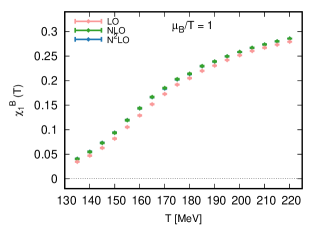
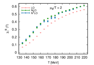
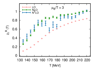
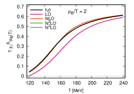
In Fig. 1 we show the baryon density $n_{B}(T)$ obtained from a Taylor expansion with the coefficients in Ref. [20], at $\hat{\mu}_{B}=1,2,3$. The extrapolation is shown including an increasing number of coefficients, to show the effect of higher-order ones. The leading-order (LO) and higher truncations refer to $\sim\hat{\mu}_{B}\partial n_{B}(T)/\partial\hat{\mu}_{B}$, or $\sim\frac{1}{6}\hat{\mu}_{B}^{3}\partial^{3}n_{B}(T)/\partial\hat{\mu}_{B}^{3}$, etc. being the last term in the expansion. The derivatives are taken at $\mu_{B}=0$.

While at $\hat{\mu}_{B}=1$ apparent convergence is achieved at the NLO level, for higher chemical potential this is not the case. Especially at $\hat{\mu}_{B}=3$, the inclusion of all the coefficients in Ref. [20] causes unphysical non-monotonic behavior. Ultimately, a pathological behaviour could also come from a finite radius of convergence. Incidentally, recent estimates on coarse lattices [52, 53], but also universality arguments [54] place the convergence in the same ball-park in $\mu_{B}$.

In this work, we present an alternative summation scheme which can better cope with the fact that the QCD transition temperature presents a $\mu_{B}$-dependence.

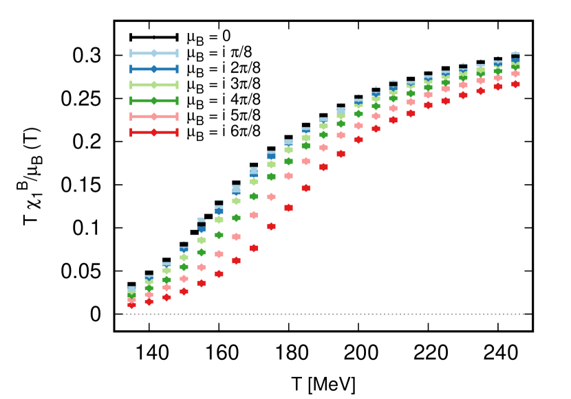
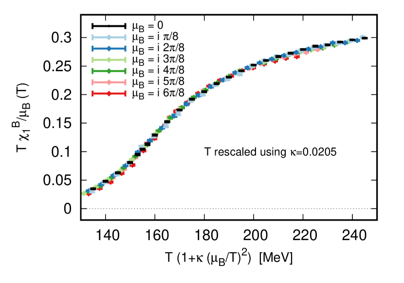
We start from the observation that we made while working with imaginary values of the chemical potentials in an earlier work on analytical continuation. In the upper panel of Fig. 2 we show temperature scans of the quantity $n_{B}(T)/\hat{\mu}_{B}=\chi^{B}_{1}(T,\hat{\mu}_{B})/\hat{\mu}_{B}$ for several fixed imaginary $\mu_{B}/T$ ratios. The $0/0$ limit at $\mu_{B}=0$ can be easily resolved and equals $\chi_{2}^{B}(T)$.

The $T$-dependence of the normalized baryon density at finite chemical potential appears to be simply shifted/rescaled towards higher temperatures from the $\mu_{B}=0$ results for $\chi_{2}^{B}$. This behavior is more apparent in the vicinity of the transition, where the slope of these curves is larger. At very large, as well as at very low temperatures a simple shift cannot describe the physics, since the curves become extremely flat. A simple rescaling of temperatures can be described as:

$$\frac{\chi_{1}^{B}(T,\hat{\mu}_{B})}{\hat{\mu}_{B}}=\chi_{2}^{B}(T^{\prime},0)\,\,,$$ (4)

where the actual temperature difference can be expressed through a $\mu_{B}$-dependent rescaling factor that we write for simplicity as

$$T^{\prime}=T\left(1+\kappa\hat{\mu}_{B}^{2}\right)\,\,.$$ (5)

In the lower panel of Fig. 2 we show a version of the curves in the upper panel, where all the finite-$\hat{\mu}_{B}$ curves have been shifted in accordance to Eq. (5) with $\kappa=0.0205$. Remarkably, we note how well the curves are superimposed to each other, even with the simple assumption of a single, $T$-independent parameter governing the transformation.

Figure 4: Benchmarking various orders of the Taylor method assuming an equation of state, where the $\mu_{B}$-dependence of $\chi^{B}_{1}/\hat{\mu}_{B}$ consists of a simple shift in temperature. This equation of state is a somewhat simplified form of the observed behaviour.

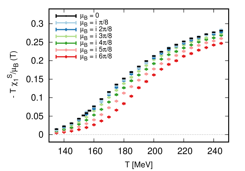
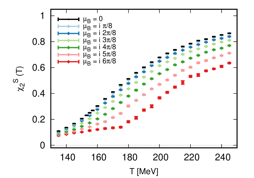
A similar behavior is observed for other quantities too. We show in Fig. 3 the first and second order fluctuations of strangeness at imaginary baryon chemical potentials. In analogy with Eq. (4) one has:

$$\frac{\chi_{1}^{S}(T,\hat{\mu}_{B})}{\hat{\mu}_{B}} =\chi_{11}^{BS}(T^{\prime},0)\,\,,$$ (6)

$$\chi_{2}^{S}(T,\hat{\mu}_{B}) =\chi_{2}^{S}(T^{\prime},0)\,\,,$$

where $T^{\prime}$ is defined analogously to Eq. (5), albeit with different $\kappa$ parameters.

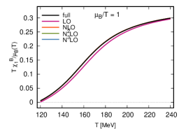
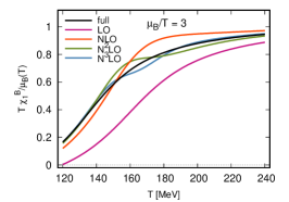
In order to motivate our alternative summation scheme, let us first consider a crude approximation that we will later refine. We take Eq. (5) at face value and use it together with Eq. (4) to obtain a well defined $\chi^{B}_{1}(T,\hat{\mu}_{B})$ function. We need a $\chi^{B}_{2}(T,0)$ function as well, which we borrow from a deliberately simple fit $f(T)=a+b\arctan(c(T-d))$ to our data on a ${{48}^{3}\!\!\times\!\!{12}}$ lattice. In principle, we could not only calculate $\chi^{B}_{1}(T,\hat{\mu}_{B})$ at arbitrary $\hat{\mu}_{B}$ but, blindly believing Eq. (5), one could calculate the higher $\mu_{B}$-derivatives as well. While this will not describe Nature precisely, it can serve as a test for the Taylor expansion method. To this end, we took several $\hat{\mu}_{B}$-derivatives of our $\chi^{B}_{1}(T,\hat{\mu}_{B})$ function and calculated its truncated Taylor series for the lowest four orders. Here LO means just plotting $\chi^{B}_{2}(T,0)$. We compared our mock curve (labelled as “full”) against its Taylor expansion at three real values of the chemical potential (see Fig. 4).

For $\hat{\mu}_{B}=1,2$, the summation up to LO and NLO is sufficient to perfectly reproduce the function. However, as the chemical potential is increased, the Taylor expansion carried as far as the NNNLO does not reproduce the original function. On the one hand, convergence is achieved more slowly; on the other hand, spurious effects appear, which generally manifest themselves in a non-monotonicity of the function. These spurious effects in truncated Taylor series were pointed out also in Refs. [55, 56, 57].

The picture emerging from this simple analysis is rather suggestive, especially when compared to the results shown in Fig. 1 (right panel) obtained from actual lattice data. We also note that this simple analysis does not suffer from the additional complications of signal extraction for higher order expansion coefficients, which in turn play a relevant role in the real-data analysis.

III Formalism

At vanishing chemical potential, it is possible to express the normalized baryon density as a Taylor expansion:

$$\frac{\chi_{1}^{B}}{\hat{\mu}_{B}}(T,\hat{\mu}_{B})=\chi_{2}^{B}(T,0)+\frac{\hat{\mu}_{B}^{2}}{6}\chi_{4}^{B}(T,0)+\frac{\hat{\mu}_{B}^{4}}{120}\chi_{6}^{B}(T,0)+\cdots$$ (7)

As we saw in Fig. 2, the behavior of $\frac{\chi_{1}^{B}}{\hat{\mu}_{B}}(T,\hat{\mu}_{B})$ at finite chemical potential clearly resembles that of $\chi_{2}^{B}(T,\hat{\mu}_{B})$, although shifted/rescaled in temperature. As long as $\chi^{B}_{1}/\hat{\mu}_{B}$ is a monotonic function of $T$, the finite density physics can be encoded into the $T^{\prime}(T,\hat{\mu}_{B})$ function. A straightforward, but systematic generalization of Eq. (5) reads:

$$T^{\prime}(T,\hat{\mu}_{B})=T\left(1+\kappa_{2}^{BB}(T)\hat{\mu}_{B}^{2}+\kappa_{4}^{BB}(T)\hat{\mu}_{B}^{4}+\mathcal{O}(\hat{\mu}_{B}^{6})\right)\,\,.$$ (8)

In the above equation, we introduced the new parameters $\kappa_{2}^{BB}(T)$ and $\kappa_{4}^{BB}(T)$, which describe the shift/rescaling of the temperature of $\chi_{1}^{B}/\hat{\mu}_{B}$ at finite $\mu_{B}$. Analogous parameters will be introduced below to for the case of $\chi_{1}^{S}/\hat{\mu}_{B}$ ($\kappa_{2}^{BS}$ and $\kappa_{4}^{BS}$) and of $\chi_{2}^{S}$ ($\kappa_{2}^{SS}$ and $\kappa_{4}^{SS}$) at finite $\mu_{B}$. In a way, this formalism replaces the fixed temperature $\mu_{B}$ expansion by a fixed-observable temperature expansion.

Having now two expressions, Eqs. (7) and (4), for the same quantity we require their equality at each order in the $\hat{\mu}_{B}$ expansion at $\mu_{B}=0$, having:

$$\chi_{4}^{B}(T) =6T\kappa_{2}^{BB}(T)\frac{d\chi_{2}}{dT}\,\,,$$ (9)

$$\chi_{6}^{B}(T) =60T^{2}(\kappa_{2}^{BB})^{2}(T)\frac{d^{2}\chi_{2}}{dT^{2}}+120T\kappa_{4}^{BB}(T)\frac{d\chi_{2}}{dT}\,\,,$$

which in turn yields:

$$\kappa_{2}^{BB}(T) =\frac{1}{6T}\frac{\chi_{4}^{B}(T)}{{\chi_{2}^{B}}^{\prime}(T)}\,\,,$$ (10)

$$\kappa_{4}^{BB}(T) =\frac{1}{360{{\chi_{2}^{B}}^{\prime}(T)}^{3}}\left(3{{\chi_{2}^{B}}^{\prime}(T)}^{2}\chi_{6}^{B}(T)-5{\chi_{2}^{B}}^{\prime\prime}(T){\chi_{4}^{B}(T)}^{2}\right)\,\,.$$

A similar treatment can be applied to the other observables. For the second order fluctuations including baryon number and strangeness, one can consider:

$$\frac{\chi_{1}^{S}}{\hat{\mu}_{B}}(T,\hat{\mu}_{B})=\chi_{11}^{BS}(T,0)+\frac{\hat{\mu}_{B}^{2}}{6}\chi_{31}^{BS}(T,0)+\frac{\hat{\mu}_{B}^{4}}{120}\chi_{51}^{BS}(T,0)+\cdots$$ (11)

and:

$$\chi_{2}^{S}(T,\hat{\mu}_{B})=\chi_{2}^{S}(T,0)+\frac{\hat{\mu}_{B}^{2}}{2}\chi_{22}^{BS}(T,0)+\frac{\hat{\mu}_{B}^{4}}{24}\chi_{42}^{BS}(T,0)+\cdots$$ (12)

Similarly as before, one can show that:

$$\kappa_{2}^{BS}(T) =\frac{1}{6T}\frac{\chi_{31}^{BS}(T)}{{\chi_{11}^{BS}}^{\prime}(T)}\,\,,$$ (13)

$$\kappa_{4}^{BS}(T) =\frac{1}{360{{\chi_{11}^{BS}}^{\prime}(T)}^{3}}\left(3{{\chi_{11}^{BS}}^{\prime}(T)}^{2}\chi_{51}^{BS}(T)\right.$$

$$\left.\qquad\qquad\qquad\qquad-5{\chi_{11}^{BS}}^{\prime\prime}(T){\chi_{31}^{BS}(T)}^{2}\right)\,\,,$$

and:

$$\kappa_{2}^{SS}(T) =\frac{1}{2T}\frac{\chi_{22}^{BS}(T)}{{\chi_{2}^{S}}^{\prime}(T)}\,\,,$$ (14)

$$\kappa_{4}^{SS}(T) =\frac{1}{24{{\chi_{2}^{S}}^{\prime}(T)}^{3}}\left({{\chi_{2}^{S}}^{\prime}(T)}^{2}\chi_{42}^{BS}(T)\right.$$

$$\left.\qquad\qquad\qquad\qquad-3{\chi_{2}^{S}}^{\prime\prime}(T){\chi_{22}^{BS}(T)}^{2}\right)\,\,.$$

Figure 5: Evaluation of Eq. (10) on a coarse lattice with high statistics. The resulting $\kappa_{2}^{BB}(T)$ shows a very mild temperature dependence in the transition region.

Before we embark into the discussion of the lattice analysis, let us have an impression on the discussed quantities. Eq. (10) gives a way to directly determine $\kappa_{2}^{BB}(T)$ and $\kappa_{4}^{BB}(T)$ using only $\mu_{B}=0$ data.

This approach might be subject to numerical problems, especially in the case of $\kappa_{4}^{BB}(T)$, which is obtained as the difference of two competing terms. Notice, too, that Eq. (10) contains temperature-derivatives of the $\chi(T)$ coefficients, which may pose a numerical challenge, unless the coefficients are known at sufficient statistics and resolution in $T$.

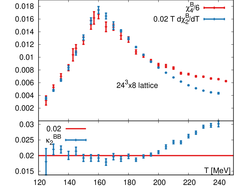
On lattices where high statistics data taking is feasible, we can investigate Eq. (10), at least for $\kappa_{2}^{BB}$. In the top panel of Fig. 5 we compare the numerator and (rescaled) denominator of Eq. (10), while their ratio $\kappa_{2}^{BB}(T)$ is shown in the bottom panel. In the entire transition region the ratio is consistent with a constant, because the peak in $\chi^{B}_{4}(T)$ is replicated in the temperature dependence of $\chi^{B}_{2}(T)$. As opposed to the Taylor coefficients, $\kappa_{2}^{BB}(T)$ shows a very mild temperature dependence.

Finally we remark that very similar equations have been already used in Ref. [14] to calculate “lines of constant physics” to $\mathcal{O}(\mu_{B}^{4})$ order. In this reference the pressure, energy density and entropy were calculated using the Taylor method, and in a further step lines were drawn on the $\mu_{B}-T$ phase diagram, where these quantities are constant in some normalization. The obtained $\kappa_{2}$ coefficients are closely related to ours.

Contrary to Ref. [14], we use Eq. (8) as the definition of a truncation scheme rather than to investigate a Taylor expanded result. In a way, we work in the opposite direction: we will use lattice data at zero and imaginary $\mu_{B}$ to obtain the coefficients in Eq. (8), which then can be used to either calculate the Taylor coefficients or, even better, to extrapolate the equation of state at finite $\mu_{B}$ with no reference to the Taylor coefficients themselves.

Also, we used imaginary chemical potentials not only to calculate the coefficients, but also to study the single observable first, on which the analysis is based. We base our description of the entire chemical potential-dependence of the QCD free energy function on $\chi_{1}^{B}(T,\hat{\mu}_{B})/\hat{\mu}_{B}$. It is essential to rely on one observable only, in order to guarantee thermodynamic consistency: entropy, pressure and energy density will obey the known thermodynamic relations (see Section V) only if they come from the same truncation scheme.

IV Lattice determination of the expansion coefficients

IV.1 Lattice details

In this work, we use the lattice action and the parameters described in Ref. [39]. The action benefits from tree-level Symanzik improvement in the gauge sector and four levels of stout smearing for the staggered flavors. The up and down quarks are degenerate. The resulting light pair of quarks, as well as the strange and charm quarks assume their respective physical mass.

We performed simulations at $\mu_{B}=0$ on $32^{3}\times 8$, $40^{3}\times 10$, $48^{3}\times 12$ and $64^{3}\times 16$ lattices in a temperature range of $130-300~{}\,{\rm MeV}$, and up to $500\,{\rm MeV}$ on larger volumes. These simulations were complemented at imaginary values of the chemical potential in the temperature range $135-245~{}\mathrm{MeV}$ for the lattice resolutions $N_{\tau}=8,\dots,12$. The $\mu_{B}\neq 0$ data were simulated at $\mu_{S}=0$, some of these ensembles were already used in Ref. [20].

In addition, we performed a high-statistics run on the cheap and coarse $24^{3}\times 8$ lattice, mainly to produce Fig. 5. These data did not enter the continuum extrapolation.

IV.2 The coefficients $\kappa_{2}^{ij}$ and $\kappa_{4}^{ij}$

Figure 6: Continuum extrapolated result for the parameters $\kappa_{2}^{BB}(T)$ and $\kappa_{4}^{BB}(T)$ (top panel), $\kappa_{2}^{BS}(T)$ and $\kappa_{4}^{BS}(T)$ (central panel), and $\kappa_{2}^{SS}(T)$ and $\kappa_{4}^{SS}(T)$ (bottom panel). The parameters $\kappa_{2}^{ij}$ are shown in blue, and the $\kappa_{4}^{ij}$ in red. HRG results for all quantities are shown up to $T=160\,{\rm MeV}$ (in green for $\kappa_{2}^{ij}$ and orange for $\kappa_{4}^{ij}$, respectively).

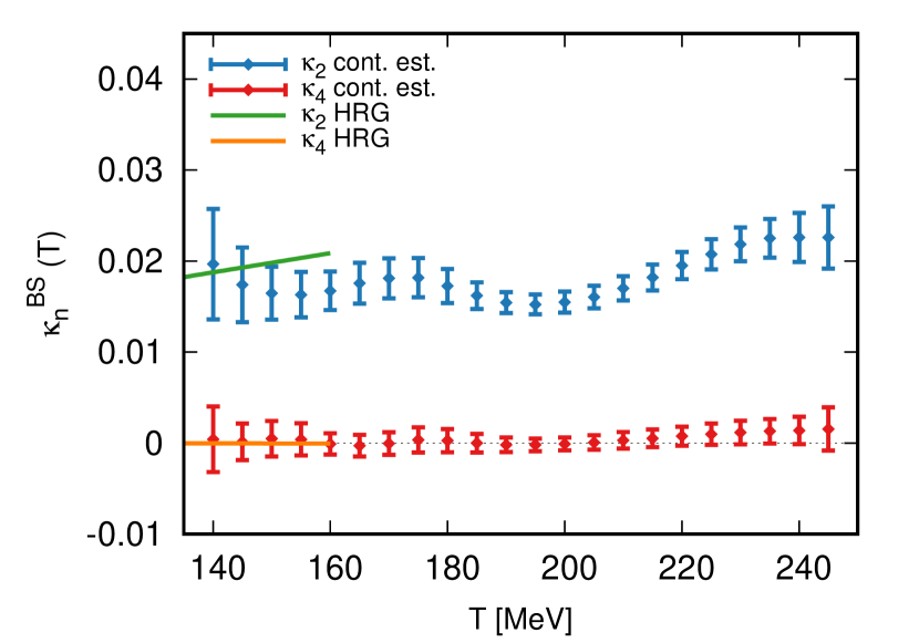
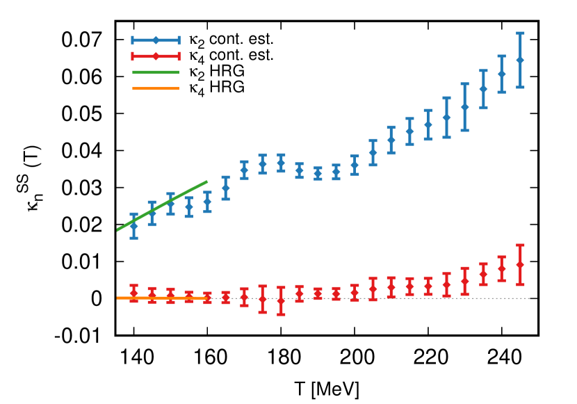
For the determination of $\kappa_{2}^{ij}$ and $\kappa_{4}^{ij}$, one can take advantage of simulations both at zero and finite imaginary chemical potential. Using Eq. (10) we calculated $\kappa_{2}^{BB}(T)$, shown in Fig. 5. To extract $\kappa_{4}^{BB}(T)$ using the same strategy, a precise result on $\chi^{6}_{B}(T)$ would be necessary.

Instead, we utilize imaginary chemical potential simulations as follows. We perform simulations at imaginary values of the baryon chemical potential:

$$\hat{\mu}_{B}=i\frac{n\pi}{8}\,\,,\qquad n\in\{3,4,5,6\}$$ (15)

with $\hat{\mu}_{Q}=\hat{\mu}_{S}=0$.

We simulate temperatures in the range $T=135-245\,{\rm MeV}$. For each temperature $T$ and chemical potential $\hat{\mu}_{B}$ we determine the temperature $T^{\prime}$ for which Eq. (7) holds, hence defining a function $T^{\prime}(T,\hat{\mu}_{B})$. Rearranging the terms in Eq (8), and in a similar way for the other observables, one can write:

$$\Pi(T,\hat{\mu}_{B}) = \kappa_{2}^{ij}(T^{\prime})+\kappa_{4}^{ij}(T^{\prime})\hat{\mu}^{2}_{B}+\kappa_{6}^{ij}(T^{\prime})\hat{\mu}^{4}_{B}+\dots\qquad$$ (16)

with the proxy quantity

$$\Pi(T,\hat{\mu}_{B}) = \frac{T^{\prime}(T,\hat{\mu}_{B})-T}{T^{\prime}(T,\hat{\mu}_{B})\hat{\mu}_{B}^{2}}.$$ (17)

The proxy $\Pi(T,\hat{\mu}_{B})$ can be determined using lattice simulations. The relatively precisely known function $\chi^{B}_{2}(T,0)$ is first interpolated in temperature. Afterwards, we only need to measure $\chi_{1}^{B}(T,\mu_{B})/\hat{\mu}_{B}$ on an ensemble with imaginary $\mu_{B}$. Equating this to $\chi^{B}_{2}(T^{\prime},0)$ gives us $T^{\prime}(T,\mu_{B})$, while we have to take care of the propagation of the statistical errors.

Having determined $\Pi(T,\hat{\mu}_{B})$ for several imaginary chemical potentials and several lattice spacings for each given temperature, one can perform a polynomial fit in $\hat{\mu}_{B}^{2}$ and obtain the expansion coefficients. This can be done separately for each lattice. However, we prefer to combine the $\hat{\mu}_{B}$ and continuum fits in one two-dimensional fitting procedure. This combined fit is repeated for every temperature, in steps of 5 MeV.

In order to estimate the systematic uncertainties associated to our results, we perform a number of analyses at each temperature. There are several ambiguous points that need to be considered. Most obviously, one could choose to include the $\kappa_{6}^{ij}(T)$ term in the fit or not, or consider the fit of $1/\Pi$ instead. Also the range in imaginary $\mu_{B}$ is arbitrary: we consider $\mathrm{Im}~{}\mu_{B}\leq 2.0$ or $\mathrm{Im}~{}\mu_{B}\leq 2.4$. When different lattice spacings are fitted together in a continuum extrapolation, one selects the bare parameters such that the ensembles correspond to the same physical temperature. This choice is, however, ambiguous too, as the scale setting may be based on various observables. In our case, we consider $f_{\pi}$ or $w_{0}$ to this purpose. As we mentioned before, $\chi^{B}_{2}(T,0)$ is subject to an interpolation, performed through basis splines. The same is true for $\chi^{B}_{1}(T,\hat{\mu}_{B})$ at finite chemical potentials. Since the location of the node points is also arbitrary, we include three versions at $\mu_{B}=0$ and two at imaginary $\mu_{B}$, each with perfect fit quality. Finally, in the continuum extrapolation the coarsest lattice, $32^{3}\times 8$, has either been used or dropped. The listed options can be considered in arbitrary combinations. In total we carry out all 144 fits to perform a continuum extrapolation of $\kappa_{2}^{ij}(T)$ and $\kappa_{4}^{ij}(T)$. After dropping the fits with a Q-value below a percent, we use uniform weights to produce histogram out of these (somewhat less than) 144 results for each temperature. The width of the histogram defines the systematic error. In the plots we show combined errors, where we assume that statistical and systematic errors add up in quadrature. This systematic error estimation procedure has been used and described in more detail in several of our works, most recently in Ref. [20].

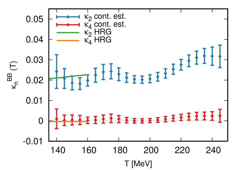
In the top panel of Fig. 6 we show the results of the temperature-by-temperature fit procedure for the parameters $\kappa_{2}^{BB}(T)$ and $\kappa_{4}^{BB}(T)$, alongside the corresponding expectations from the Hadron Resonance Gas (HRG) model. We find that, within errors, $\kappa_{2}^{BB}(T)$ has hardly any dependence on the temperature, while $\kappa_{4}^{BB}(T)$ is everywhere consistent with zero at our current level of precision. Nonetheless, a clear separation of almost one order of magnitude appears between these two coefficients. We also note that good agreement with the HRG results is found up to at least $T=160\,{\rm MeV}$.

In the central and bottom panels of Fig. 6 we show our results for the parameters $\kappa_{2}^{BS}$, $\kappa_{4}^{BS}$ and $\kappa_{2}^{SS}$, $\kappa_{4}^{SS}$ respectively, together with their HRG determinations. While for $\chi_{11}^{BS}$ barely any temperature dependence is observed, as in the case of $\chi_{2}^{B}$, for $\chi_{2}^{S}$ a much stronger $T$-dependence is clearly visible. As in the case of $\kappa_{4}^{BB}$, $\kappa_{4}^{BS}$ is consistent with zero throughout the whole temperature range we consider. On the other hand, $\kappa_{4}^{SS}$ rises above zero for temperatures $T\gtrsim 220\,{\rm MeV}$.

Figure 7: Results of the polynomial fits to $\kappa_{2}^{BB}$ and $\kappa_{4}^{BB}$ (top panel), $\kappa_{2}^{BS}(T)$ and $\kappa_{4}^{BS}(T)$ (central panel), and $\kappa_{2}^{SS}(T)$ and $\kappa_{4}^{SS}(T)$ (bottom panel). The parameters $\kappa_{2}^{ij}$ are shown in blue, and the $\kappa_{4}^{ij}$ in red. The fitted quantities from Fig. 6 are shown by lighter blue and red points. Due to the lack of points at low $T$, we continued the data set with HRG points, show as green and orange dots. Though the polynomials do not always follow all “excursions” of the $T$-by-$T$ result, the reduced $\chi^{2}$ of the correlated temperature fit is always $<1$. This is possible, because the fitted data are highly correlated, coming from both statistical and systematic effects.

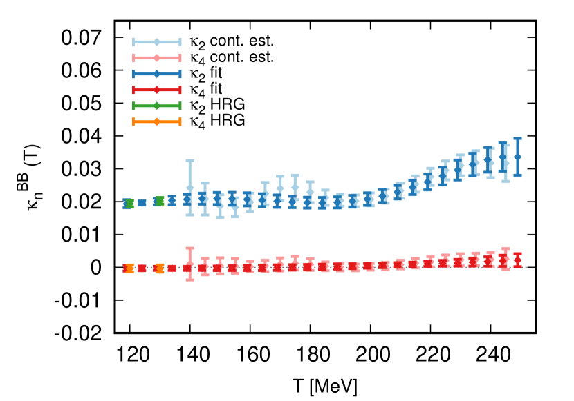
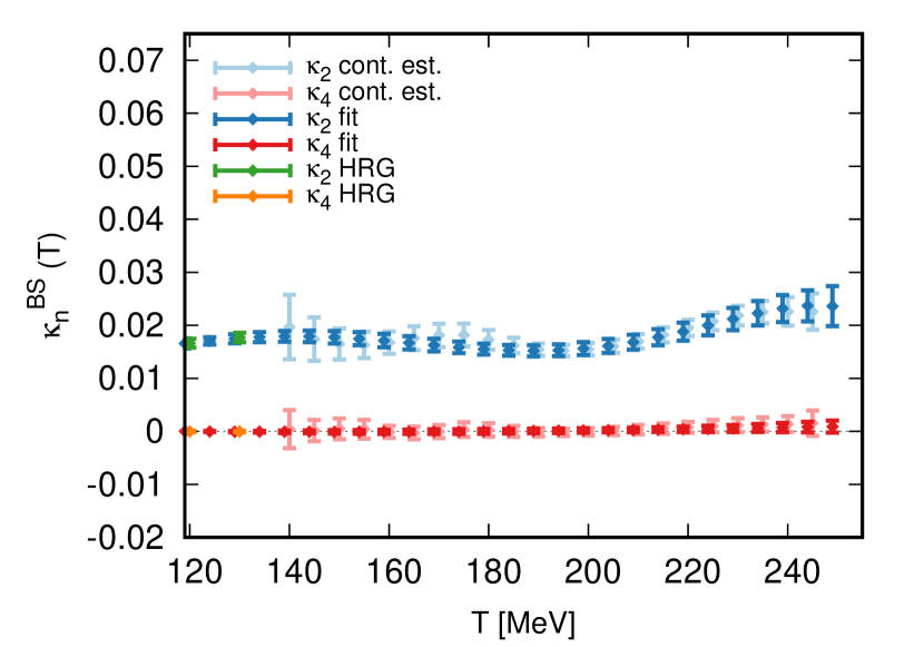
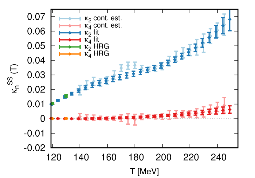
Note that the error bars in these plots are highly correlated. The correlation is mostly systematic. The apparent ‘waves’ are often statistically not as significant as it seems at a first glance. For comparison we refer to the direct result on our coarsest lattice in Fig. 5, where these ‘waves’ are absent. Before moving on to calculate thermodynamic observables at finite real chemical potential, we construct a smoother version of our final results for $\kappa_{2}^{ij}$ and $\kappa_{4}^{ij}$, in order to limit the influence of numerical effects on the final observables, but also to facilitate the temperature derivatives that enter the entropy formula. Thanks to the very mild dependence of the coefficients on the temperature, we perform a polynomial fit of order 5 for the $\kappa_{2}^{ij}$, and of order 2 for the even less $T$-dependent $\kappa_{4}^{ij}$. The very good fit qualities did not motivate higher order polynomials, using fourth or sixth order for $\kappa_{2}^{ij}$ hardly changes the result. In order to stabilize the low-temperature behavior, we include in the fit two points from the HRG model for $T=120,130\,{\rm MeV}$, to which we associate an uncertainty of $5\%$ for $\kappa_{2}^{ij}$ and of $300\%$ for $\kappa_{4}^{ij}$. The choice of these particular values for the uncertainties is uniquely guided by the necessity of placing a constraint on the low-T behavior, while avoiding to drive the fit too strongly. For this reason, these arbitrary errors are chosen to be smaller, but comparable to the lattice ones. We note that the fits we perform take fully into account the correlations between results at different temperatures, systematic as well as statistical. Thus we encode all errors into the (correlated) errors of the coefficients of a polynomial.

In Fig. 7 we show the results of the fits in darker color, with the fitted data in lighter shades. The HRG points included in the fit are shown as well.

IV.3 Continuum result on $\chi^{B}_{2}(T)$ and its temperature derivative

Figure 8: Continuum extrapolated $\chi^{B}_{2}(T)$ and $Td\chi^{B}_{2}(T)/dT$ functions from $N_{\tau}=10$, 12 and 16 lattices at $\mu_{B}=0$. Together with $\kappa^{BB}_{n}(T)$ these functions enter the thermodynamic analysis.

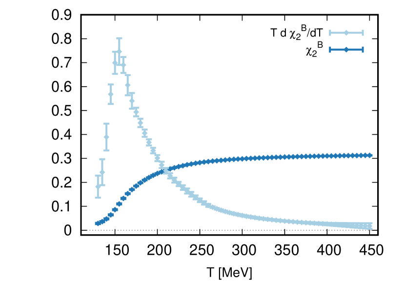
In order to determine the value of thermodynamic quantities at finite real chemical potential, a continuum result for the basic quantity $\chi^{B}_{2}(T,0)$ is required in addition to $\kappa_{2}^{BB}(T)$ and $\kappa_{4}^{BB}(T)$. For some observables like the entropy, the temperature derivative of $\chi^{B}_{2}(T)$ has to be calculated as well. We have already published this quantity in Ref. [39], but not its temperature derivatives. To make this work self-contained, we update this determination with the updated statistics using lattices up to $64^{3}\times 16$.

We have divided the temperature range into two parts: the transition region and the higher, near-perturbative temperatures. For the lower temperature part, we interpolate using basis splines using the $T\in[130~{}\mathrm{MeV},300~{}\mathrm{MeV}]$ data points. For the quantity $Td\chi^{B}_{2}(T)/dT$ we extended the data range with the HRG curve, so that the numerical derivative has a level arm at the lowest temperatures. The basis splines are cubic splines in the given temperature range. We fit the splines in temperature and in $1/N_{\tau}^{2}$ in one step. The fitted function in this range is thus:

$$\chi^{B}_{2}(T,0;N_{\tau})=\sum_{i=1}^{n}\alpha_{i}b_{i}(T)+\frac{1}{N_{\tau}^{2}}\sum_{i=1}^{n}\beta_{i}b_{i}(T)\,,$$ (18)

where $b_{i}(t_{j})=\delta_{ij}$ and $t_{j}$ are the knots for the spline with $j=1\dots n$. $n$ and the $t_{j}$ set are the only arbitrary inputs. We combine the result from four sets of values for them, so that we can estimate the systematics. Only the lattices with $N_{\tau}=10,12$ and 16 enter the continuum extrapolation. For $\chi^{B}_{2}(T,0;N_{\tau})$ in Eq. (18), the tree-level improvement was already applied [39]. The lattice resolutions and the spline knots are selected such that the fit qualities (Q value) are distributed as expected. We also took into account the scale setting ambiguity by combining the results with $w_{0}-$ and $f_{\pi}-$based scale settings. The systematics of the $T$-derivative $Td\chi^{B}_{2}(T,0)/dT$ and of $\chi^{B}_{2}(T,0)$ were determined separately.

In the high temperature regime, the smooth monotonic behavior is not well described with cubic splines. Instead we performed a high order polynomial fit in the inverse temperature $1/T$. The known analytical form of the convergence to the Stefan-Boltzmann limit is, of course, not this polynomial. We do not wish to enforce the perturbative behavior at the intermediate temperatures that we describe. Thus, the constant in the $1/T$ description is not exactly the Stefan-Boltzmann limit, and for this reason, we cannot regard this as a basis for an extrapolation. However, this simple approach allows the interpolation and the calculation of the derivative. We used lattice data in the range $T=180-450~{}\mathrm{MeV}$.

High- and low-temperature regions overlap and the two fitting methods give consistent results between $T=200-280\,{\rm MeV}$ for both quantities. Thus, we simply concatenate the resulting functions at $T=260\,{\rm MeV}$. We show the final version of the $Td\chi^{B}_{2}(T,0)/dT$ and $\chi^{B}_{2}(T,0)$ functions in Fig. 8.

V Thermodynamics at real chemical potential

Figure 9: Baryon density, pressure, entropy, energy density, strangeness density and $\chi_{2}^{S}$ at increasing values of $\hat{\mu}_{B}$. With solid lines we show the results from the HRG model.

Once $n_{B}$ is determined, we have everything we need to extract the other thermodynamic quantities. The integration constant for the pressure is obviously the pressure itself at $\mu_{B}=0$.

We note here that, on the lattice, we always deal with dimensionless thermodynamic quantities, which correspond to the physical ones divided by suitable powers of the temperature. E.g., the dimensionful baryon density is $n_{B}=T^{3}\hat{n}_{B}$ (we will hereafter use the hat to indicate dimensionless quantities).

From the baryon density $\hat{n}_{B}(\hat{\mu}_{B},T)$, the pressure is obtained through simple integration:

$$\frac{p(\mu_{B},T)}{T^{4}}=\hat{p}(\hat{\mu}_{B},T)=\hat{p}(0,T)+\bigintssss_{0}^{\hat{\mu}_{B}}\!\!\!\!\!\!{\rm d}\hat{\mu}^{\prime}_{B}\,\hat{n}_{B}(\hat{\mu}_{B}^{\prime},T)\,\,.$$ (19)

The entropy density is defined as:

$$s(\mu_{B},T)=\left.\frac{\partial p(\mu_{B},T)}{\partial T}\right|_{\mu}.$$ (20)

For dimensionless quantities:

$$\hat{s}(\hat{\mu}_{B},T) =4\,\hat{p}(\hat{\mu}_{B},T)+T\left.\frac{\partial\hat{p}(\hat{\mu}_{B},T)}{\partial T}\right|_{\mu}=$$ (21)

$$=4\,\hat{p}(\hat{\mu}_{B},T)+T\left.\frac{\partial\hat{p}(\hat{\mu}_{B},T)}{\partial T}\right|_{\hat{\mu}}-\hat{\mu}_{B}\hat{n}_{B}(\hat{\mu}_{B},T)$$

where in the last step we converted the derivative at constant $\mu_{B}$ into a derivative at constant $\hat{\mu}_{B}$.

The $T$-derivative of the pressure involves the chain rule

$$\quad T\left.\frac{\partial\hat{p}(\hat{\mu}_{B},T)}{\partial T}\right|_{\hat{\mu}}=T\left.\frac{\partial\hat{p}(0,T)}{\partial T}\right|_{\hat{\mu}}$$ (22)

$$\quad\qquad+\frac{1}{2}\int_{0}^{\hat{\mu}_{B}^{2}}T\left.\frac{d\chi^{B}_{2}(T^{\prime})}{dT^{\prime}}\right|_{T^{\prime}=T\left(1+\kappa_{2}^{BB}y+\kappa_{4}^{BB}y^{2}\right)}\times$$

$$\quad\times\left[1+\kappa_{2}^{BB}y+\kappa_{4}^{BB}y^{2}+T\left(\frac{d\kappa_{2}^{BB}}{dT}y+\frac{d\kappa_{4}^{BB}}{dT}y^{2}\right)\right]dy$$

where $\frac{d\chi^{B}_{2}(T)}{dT}$ is calculated at $\mu_{B}=0$ as already described.

The dimensionless expression for the energy density $\hat{\epsilon}=\epsilon/T^{4}$ follows as:

$$\hat{\epsilon}(\hat{\mu}_{B},T)=\hat{s}(\hat{\mu}_{B},T)-\hat{p}(\hat{\mu}_{B},T)+\hat{\mu}_{B}\hat{n}_{B}(\hat{\mu}_{B},T).$$ (23)

Figure 10: Comparison of baryon density (left) and energy density (right) at different values of $\hat{\mu}_{B}$ in the case where a $\kappa_{4}^{BB}$ parameter is used (darker shades) or omitted (lighter shades). The HRG results are shown with solid lines.

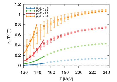
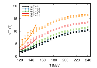
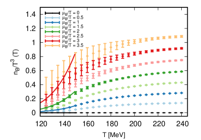
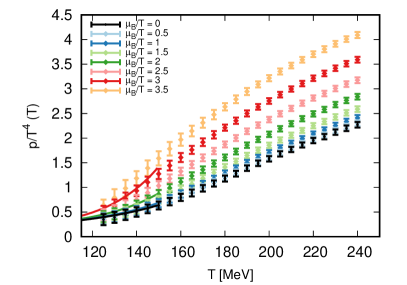
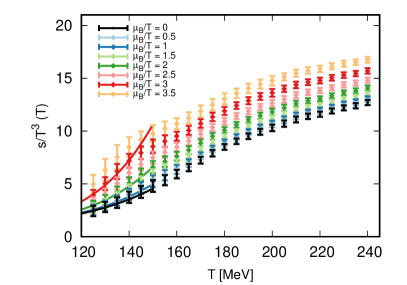
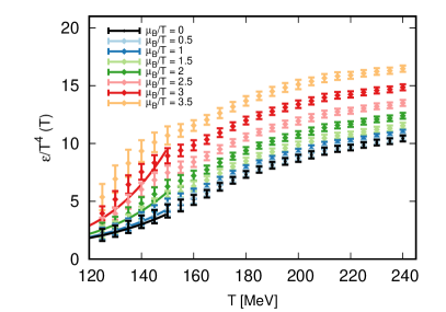
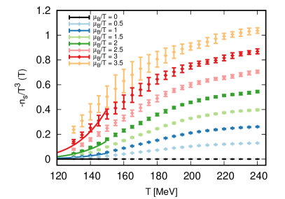
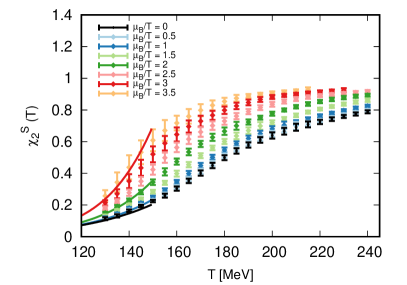
Finally, we present our results for the finite real chemical potential extrapolation of several thermodynamic quantities. The various panels of Fig. 9 show the baryon density, pressure, entropy, energy density, strangeness density and $\chi_{2}^{S}$ for $\hat{\mu}_{B}=0-3.5$. Alongside our results, we show predictions from the HRG model for $T<150\,{\rm MeV}$, which we find in very good agreement with our extrapolation for all observables, at all values of the chemical potential.

We also note that in all cases, the observables do not suffer from pathological behavior. The uncertainties are under control for our range of chemical potentials, which highly improves on the results currently achievable via Taylor expansion.

We devote the two panels of Fig. 10 to the comparison of our results for the baryon density (left) and energy density (right) to the simplified case where $\kappa_{4}^{BB}$ is neglected. We can appreciate how the inclusion of the next-to-leading-order parameter came at the cost of an increased uncertainty at larger chemical potential. This does not come unexpected, as we saw from our results that $\kappa_{4}^{BB}$ was compatible with zero at all temperatures. In the case of the energy density, which is dominated by the $\mu_{B}=0$ contribution, hardly any effect is visible.

VI Conclusions

In this work, we proposed an alternative summation scheme for the equation of state of QCD at finite real chemical potential, designed to overcome the shortcomings which are characteristic of the Taylor expansion approach. Combining simulations at both zero and imaginary chemical potentials, we determined the LO and NLO parameters describing the chemical potential dependence of the baryon density, which we could then extrapolate to large real chemical potentials.

By combining this new element, and previously published results for the EoS at vanishing density, we could reconstruct all thermodynamic variables at chemical potentials as large as $\mu_{B}/T=3.5$ with rather limited uncertainty. Systematic as well as statistical errors were considered in the analysis.

These results, although still limited in precision at the level of the parameters $\kappa_{2}^{ij}$ and $\kappa_{4}^{ij}$, suggest that the avenue we pursue in this work is rather promising for the description of QCD thermodynamics at finite chemical potential. Moreover, our procedure is systematically improvable with sufficient computing power, and might prove to be a better strategy than existing “canonical” approaches.

In this work we limited ourselves to the case where the strange and electric chemical potentials are set to zero. We reserve for future work the exploration of the phenomenologically relevant case of strangeness neutrality and fixed electric charge to baryon ratio.

Acknowledgments

This project was funded by the DFG grant SFB/TR55. The project also received support from the BMBF Grant No. 05P18PXFCA. This work was also supported by the Hungarian National Research, Development and Innovation Office, NKFIH grant KKP126769. A.P. is supported by the J. Bolyai Research Scholarship of the Hungarian Academy of Sciences and by the ÚNKP-20-5 New National Excellence Program of the Ministry for Innovation and Technology. The project leading to this publication has received funding from Excellence Initiative of Aix-Marseille University - A*MIDEX, a French “Investissements d’Avenir” programme, AMX-18-ACE-005. This material is based upon work supported by the National Science Foundation under grants no. PHY-1654219 and by the U.S. DoE, Office of Science, Office of Nuclear Physics, within the framework of the Beam Energy Scan Topical (BEST) Collaboration. This research used resources of the Oak Ridge Leadership Computing Facility, which is a DOE Office of Science User Facility supported under Contract DE-AC05-00OR22725. The authors gratefully acknowledge the Gauss Centre for Supercomputing e.V. (www.gauss-centre.eu) for funding this project by providing computing time on the GCS Supercomputer HAWK at HLRS, Stuttgart. Part of the computation was performed on the QPACE3 funded by the DFG ind hosted by JSC. C.R. also acknowledges the support from the Center of Advanced Computing and Data Systems at the University of Houston.

References

- Aoki et al. [2006] Y. Aoki, G. Endrodi, Z. Fodor, S. D. Katz, and K. K. Szabo, The Order of the quantum chromodynamics transition predicted by the standard model of particle physics, Nature 443, 675 (2006), arXiv:hep-lat/0611014 [hep-lat] .
- Guenther [2020] J. N. Guenther, Overview of the QCD phase diagram - Recent progress from the lattice, (2020), arXiv:2010.15503 [hep-lat] .
- Ratti [2018] C. Ratti, Lattice QCD and heavy ion collisions: a review of recent progress, Rept. Prog. Phys. 81, 084301 (2018), arXiv:1804.07810 [hep-lat] .
- Cristoforetti et al. [2012] M. Cristoforetti, F. Di Renzo, and L. Scorzato (AuroraScience), New approach to the sign problem in quantum field theories: High density QCD on a Lefschetz thimble, Phys. Rev. D 86, 074506 (2012), arXiv:1205.3996 [hep-lat] .
- Alexandru et al. [2016] A. Alexandru, G. Basar, and P. Bedaque, Monte Carlo algorithm for simulating fermions on Lefschetz thimbles, Phys. Rev. D 93, 014504 (2016), arXiv:1510.03258 [hep-lat] .
- Fukuma et al. [2019] M. Fukuma, N. Matsumoto, and N. Umeda, Implementation of the HMC algorithm on the tempered Lefschetz thimble method, (2019), arXiv:1912.13303 [hep-lat] .
- Aarts et al. [2013] G. Aarts, F. A. James, J. M. Pawlowski, E. Seiler, D. Sexty, and I.-O. Stamatescu, Stability of complex Langevin dynamics in effective models, JHEP 03, 073, arXiv:1212.5231 [hep-lat] .
- Sexty [2014] D. Sexty, Simulating full QCD at nonzero density using the complex Langevin equation, Phys. Lett. B 729, 108 (2014), arXiv:1307.7748 [hep-lat] .
- Scherzer et al. [2020] M. Scherzer, E. Seiler, D. Sexty, and I.-O. Stamatescu, Controlling Complex Langevin simulations of lattice models by boundary term analysis, Phys. Rev. D 101, 014501 (2020), arXiv:1910.09427 [hep-lat] .
- Giordano et al. [2020a] M. Giordano, K. Kapas, S. D. Katz, D. Nogradi, and A. Pasztor, New approach to lattice QCD at finite density; results for the critical end point on coarse lattices, JHEP 05, 088, arXiv:2004.10800 [hep-lat] .
- Allton et al. [2002] C. R. Allton, S. Ejiri, S. J. Hands, O. Kaczmarek, F. Karsch, E. Laermann, C. Schmidt, and L. Scorzato, The QCD thermal phase transition in the presence of a small chemical potential, Phys. Rev. D66, 074507 (2002), arXiv:hep-lat/0204010 [hep-lat] .
- Allton et al. [2005] C. R. Allton, M. Doring, S. Ejiri, S. J. Hands, O. Kaczmarek, F. Karsch, E. Laermann, and K. Redlich, Thermodynamics of two flavor QCD to sixth order in quark chemical potential, Phys. Rev. D71, 054508 (2005), arXiv:hep-lat/0501030 [hep-lat] .
- Borsanyi et al. [2012] S. Borsanyi, G. Endrodi, Z. Fodor, S. D. Katz, S. Krieg, C. Ratti, and K. K. Szabo, QCD equation of state at nonzero chemical potential: continuum results with physical quark masses at order , JHEP 08, 053, arXiv:1204.6710 [hep-lat] .
- Bazavov et al. [2017] A. Bazavov et al., The QCD Equation of State to from Lattice QCD, Phys. Rev. D95, 054504 (2017), arXiv:1701.04325 [hep-lat] .
- Kaczmarek et al. [2011] O. Kaczmarek, F. Karsch, E. Laermann, C. Miao, S. Mukherjee, P. Petreczky, C. Schmidt, W. Soeldner, and W. Unger, Phase boundary for the chiral transition in (2+1) -flavor QCD at small values of the chemical potential, Phys. Rev. D83, 014504 (2011), arXiv:1011.3130 [hep-lat] .
- Endrodi et al. [2011] G. Endrodi, Z. Fodor, S. D. Katz, and K. K. Szabo, The QCD phase diagram at nonzero quark density, JHEP 04, 001, arXiv:1102.1356 [hep-lat] .
- Bonati et al. [2018] C. Bonati, M. D’Elia, F. Negro, F. Sanfilippo, and K. Zambello, Curvature of the pseudocritical line in QCD: Taylor expansion matches analytic continuation, Phys. Rev. D98, 054510 (2018), arXiv:1805.02960 [hep-lat] .
- Bazavov et al. [2019] A. Bazavov et al. (HotQCD), Chiral crossover in QCD at zero and non-zero chemical potentials, Phys. Lett. B795, 15 (2019), arXiv:1812.08235 [hep-lat] .
- D’Elia et al. [2017] M. D’Elia, G. Gagliardi, and F. Sanfilippo, Higher order quark number fluctuations via imaginary chemical potentials in QCD, Phys. Rev. D 95, 094503 (2017), arXiv:1611.08285 [hep-lat] .
- Borsanyi et al. [2018] S. Borsanyi, Z. Fodor, J. N. Guenther, S. K. Katz, K. K. Szabo, A. Pasztor, I. Portillo, and C. Ratti, Higher order fluctuations and correlations of conserved charges from lattice QCD, JHEP 10, 205, arXiv:1805.04445 [hep-lat] .
- de Forcrand and Philipsen [2002] P. de Forcrand and O. Philipsen, The QCD phase diagram for small densities from imaginary chemical potential, Nucl. Phys. B642, 290 (2002), arXiv:hep-lat/0205016 [hep-lat] .
- D’Elia and Lombardo [2003] M. D’Elia and M.-P. Lombardo, Finite density QCD via imaginary chemical potential, Phys. Rev. D67, 014505 (2003), arXiv:hep-lat/0209146 [hep-lat] .
- D’Elia et al. [2007] M. D’Elia, F. Di Renzo, and M. P. Lombardo, The Strongly interacting quark gluon plasma, and the critical behaviour of QCD at imaginary mu, Phys. Rev. D76, 114509 (2007), arXiv:0705.3814 [hep-lat] .
- Cea et al. [2009a] P. Cea, L. Cosmai, M. D’Elia, C. Manneschi, and A. Papa, Analytic continuation of the critical line: Suggestions for QCD, Phys. Rev. D 80, 034501 (2009a), arXiv:0905.1292 [hep-lat] .
- Cea et al. [2009b] P. Cea, L. Cosmai, M. D’Elia, C. Manneschi, and A. Papa, On the analytic continuation of the critical line, PoS LAT2009, 161 (2009b), arXiv:1001.4439 [hep-lat] .
- Bonati et al. [2014] C. Bonati, M. D’Elia, P. de Forcrand, O. Philipsen, and F. Sanfilippo, The chiral phase transition for two-flavour QCD at imaginary and zero chemical potential, PoS LATTICE2013, 219 (2014), arXiv:1311.0473 [hep-lat] .
- Bonati et al. [2015] C. Bonati, M. D’Elia, M. Mariti, M. Mesiti, F. Negro, and F. Sanfilippo, Curvature of the chiral pseudocritical line in QCD: Continuum extrapolated results, Phys. Rev. D92, 054503 (2015), arXiv:1507.03571 [hep-lat] .
- Cea et al. [2016] P. Cea, L. Cosmai, and A. Papa, Critical line of 2+1 flavor QCD: Toward the continuum limit, Phys. Rev. D93, 014507 (2016), arXiv:1508.07599 [hep-lat] .
- Bellwied et al. [2015a] R. Bellwied, S. Borsanyi, Z. Fodor, J. Guenther, S. D. Katz, C. Ratti, and K. K. Szabo, The QCD phase diagram from analytic continuation, Phys. Lett. B751, 559 (2015a), arXiv:1507.07510 [hep-lat] .
- Borsanyi et al. [2020] S. Borsanyi, Z. Fodor, J. N. Guenther, R. Kara, S. D. Katz, P. Parotto, A. Pasztor, C. Ratti, and K. K. Szabo, QCD Crossover at Finite Chemical Potential from Lattice Simulations, Phys. Rev. Lett. 125, 052001 (2020), arXiv:2002.02821 [hep-lat] .
- Karsch et al. [2011] F. Karsch, B.-J. Schaefer, M. Wagner, and J. Wambach, Towards finite density QCD with Taylor expansions, Phys. Lett. B 698, 256 (2011), arXiv:1009.5211 [hep-ph] .
- Cea et al. [2012] P. Cea, L. Cosmai, M. D’Elia, A. Papa, and F. Sanfilippo, The critical line of two-flavor QCD at finite isospin or baryon densities from imaginary chemical potentials, Phys. Rev. D 85, 094512 (2012), arXiv:1202.5700 [hep-lat] .
- Datta et al. [2017] S. Datta, R. V. Gavai, and S. Gupta, Quark number susceptibilities and equation of state at finite chemical potential in staggered QCD with Nt=8, Phys. Rev. D95, 054512 (2017), arXiv:1612.06673 [hep-lat] .
- Pásztor et al. [2020] A. Pásztor, Z. Szép, and G. Markó, Apparent convergence of Pad\’e approximants for the crossover line in finite density QCD, (2020), arXiv:2010.00394 [hep-lat] .
- Schmidt et al. [2021] C. Schmidt, J. Goswami, G. Nicotra, F. Ziesché, P. Dimopoulos, F. Di Renzo, S. Singh, and K. Zambello, Net-baryon number fluctuations, in Criticality in QCD and the Hadron Resonance Gas (2021) arXiv:2101.02254 [hep-lat] .
- Mogliacci et al. [2013] S. Mogliacci, J. O. Andersen, M. Strickland, N. Su, and A. Vuorinen, Equation of State of hot and dense QCD: Resummed perturbation theory confronts lattice data, JHEP 12, 055, arXiv:1307.8098 [hep-ph] .
- Haque et al. [2014] N. Haque, J. O. Andersen, M. G. Mustafa, M. Strickland, and N. Su, Three-loop HTLpt Pressure and Susceptibilities at Finite Temperature and Density, Phys.Rev. D89, 061701 (2014), arXiv:1309.3968 [hep-ph] .
- Haque and Strickland [2020] N. Haque and M. Strickland, NNLO HTLpt predictions for the curvature of the QCD phase transition line, (2020), arXiv:2011.06938 [hep-ph] .
- Bellwied et al. [2015b] R. Bellwied, S. Borsanyi, Z. Fodor, S. D. Katz, A. Pasztor, C. Ratti, and K. K. Szabo, Fluctuations and correlations in high temperature QCD, Phys. Rev. D92, 114505 (2015b), arXiv:1507.04627 [hep-lat] .
- Ding et al. [2015] H. T. Ding, S. Mukherjee, H. Ohno, P. Petreczky, and H. P. Schadler, Diagonal and off-diagonal quark number susceptibilities at high temperatures, Phys. Rev. D92, 074043 (2015), arXiv:1507.06637 [hep-lat] .
- Pratt et al. [2015] S. Pratt, E. Sangaline, P. Sorensen, and H. Wang, Constraining the Eq. of State of Super-Hadronic Matter from Heavy-Ion Collisions, Phys. Rev. Lett. 114, 202301 (2015), arXiv:1501.04042 [nucl-th] .
- Borsanyi et al. [2010] S. Borsanyi, G. Endrodi, Z. Fodor, A. Jakovac, S. D. Katz, S. Krieg, C. Ratti, and K. K. Szabo, The QCD equation of state with dynamical quarks, JHEP 11, 077, arXiv:1007.2580 [hep-lat] .
- Borsanyi et al. [2014] S. Borsanyi, Z. Fodor, C. Hoelbling, S. D. Katz, S. Krieg, and K. K. Szabo, Full result for the QCD equation of state with 2+1 flavors, Phys. Lett. B730, 99 (2014), arXiv:1309.5258 [hep-lat] .
- Bazavov et al. [2014] A. Bazavov et al. (HotQCD), Equation of state in ( 2+1 )-flavor QCD, Phys. Rev. D90, 094503 (2014), arXiv:1407.6387 [hep-lat] .
- Gunther et al. [2017] J. Gunther, R. Bellwied, S. Borsanyi, Z. Fodor, S. D. Katz, A. Pasztor, and C. Ratti, The QCD equation of state at finite density from analytical continuation, Proceedings, 12th Conference on Quark Confinement and the Hadron Spectrum (Confinement XII): Thessaloniki, Greece, EPJ Web Conf. 137, 07008 (2017), arXiv:1607.02493 [hep-lat] .
- Bazavov et al. [2020] A. Bazavov et al., Skewness, kurtosis, and the fifth and sixth order cumulants of net baryon-number distributions from lattice QCD confront high-statistics STAR data, Phys. Rev. D 101, 074502 (2020), arXiv:2001.08530 [hep-lat] .
- Fu et al. [2021] W.-j. Fu, X. Luo, J. M. Pawlowski, F. Rennecke, R. Wen, and S. Yin, Hyper-order baryon number fluctuations at finite temperature and density, (2021), arXiv:2101.06035 [hep-ph] .
- Bellwied et al. [2020] R. Bellwied, S. Borsanyi, Z. Fodor, J. N. Guenther, J. Noronha-Hostler, P. Parotto, A. Pasztor, C. Ratti, and J. M. Stafford, Off-diagonal correlators of conserved charges from lattice QCD and how to relate them to experiment, Phys. Rev. D 101, 034506 (2020), arXiv:1910.14592 [hep-lat] .
- Noronha-Hostler et al. [2019] J. Noronha-Hostler, P. Parotto, C. Ratti, and J. M. Stafford, Lattice-based equation of state at finite baryon number, electric charge and strangeness chemical potentials, Phys. Rev. C 100, 064910 (2019), arXiv:1902.06723 [hep-ph] .
- Monnai et al. [2019] A. Monnai, B. Schenke, and C. Shen, Equation of state at finite densities for QCD matter in nuclear collisions, Phys. Rev. C 100, 024907 (2019), arXiv:1902.05095 [nucl-th] .
- Friman et al. [2011] B. Friman, F. Karsch, K. Redlich, and V. Skokov, Fluctuations as probe of the QCD phase transition and freeze-out in heavy ion collisions at LHC and RHIC, Eur.Phys.J. C71, 1694 (2011), arXiv:1103.3511 [hep-ph] .
- Giordano and Pásztor [2019] M. Giordano and A. Pásztor, Reliable estimation of the radius of convergence in finite density QCD, Phys. Rev. D 99, 114510 (2019), arXiv:1904.01974 [hep-lat] .
- Giordano et al. [2020b] M. Giordano, K. Kapas, S. D. Katz, D. Nogradi, and A. Pasztor, Radius of convergence in lattice QCD at finite with rooted staggered fermions, Phys. Rev. D 101, 074511 (2020b), arXiv:1911.00043 [hep-lat] .
- Connelly et al. [2021] A. Connelly, G. Johnson, S. Mukherjee, and V. Skokov, Universality driven analytic structure of QCD crossover: radius of convergence and QCD critical point, Nucl. Phys. A 1005, 121834 (2021), arXiv:2004.05095 [hep-ph] .
- Ratti et al. [2007] C. Ratti, S. Roessner, and W. Weise, Quark number susceptibilities: Lattice QCD versus PNJL model, Phys. Lett. B 649, 57 (2007), arXiv:hep-ph/0701091 .
- Critelli et al. [2017] R. Critelli, J. Noronha, J. Noronha-Hostler, I. Portillo, C. Ratti, and R. Rougemont, Critical point in the phase diagram of primordial quark-gluon matter from black hole physics, Phys. Rev. D 96, 096026 (2017), arXiv:1706.00455 [nucl-th] .
- Parotto et al. [2020] P. Parotto, M. Bluhm, D. Mroczek, M. Nahrgang, J. Noronha-Hostler, K. Rajagopal, C. Ratti, T. Schäfer, and M. Stephanov, QCD equation of state matched to lattice data and exhibiting a critical point singularity, Phys. Rev. C 101, 034901 (2020), arXiv:1805.05249 [hep-ph] .