Non-local reparametrization action in coupled Sachdev–Ye–Kitaev models

Abstract

We continue the investigation of coupled Sachdev–Ye–Kitaev(SYK) models without Schwarzian action dominance. Like the original SYK, at large $N$ and low energies these models have an approximate reparametrization symmetry. However, the dominant action for reparametrizations is non-local due to the presence of irrelevant local operator with small conformal dimension. We semi-analytically study different thermodynamic properties and the 4-point function and demonstrate that they significantly differ from the Schwarzian prediction. However, the residual entropy and maximal chaos exponent are the same as in Majorana SYK. We also discuss chain models and finite $N$ corrections.

1 Introduction

Sachdev–Ye–Kitaev(SYK) model SachdevYe ; KitaevTalks ; Gross:2016kjj and related Kondo models parcollet1998 ; GPS and tensor models Gurau:2009tw ; Witten:2016iux ; Klebanov:2016xxf ; Klebanov:2017nlk are remarkable quantum mechanical models which exhibit emergent conformal symmetry, maximal chaos Maldacena:2015waa and non-zero residual entropy. The most salient feature shared by all these models is the emergence of reparametrization symmetry at low energies which is explicitly(by kinetic term) and spontaneously(by the form of 2-point function) broken. It was shown by Maldacena and Stanford ms and Kitaev and Suh SuhFirstPaper that in the original SYK model the corresponding (Euclidean) action for reparametrizations is governed by the Schwarzian action:

$$S_{Sch}=-\frac{N\alpha^{S}_{Sch}}{J}\int du\ \operatorname*{Sch}\left(\tau[u],u\right),\ \operatorname*{Sch}\left(\tau[u],u\right)=\frac{\tau^{\prime\prime\prime}}{\tau^{\prime}}-\frac{3}{2}\left(\frac{\tau^{\prime\prime}}{\tau^{\prime}}\right)^{2}.$$ (1)

Because of this it has been conjectured that the original SYK model provides a UV completion for two-dimensional Jackiw–Teitelboim (JT) gravity.

In a variety of examples it has been explicitly demonstrated that the Schwarzian does indeed dominate in various physical observables at low energies in both in- and out-of-equilibrium. However, it had remained an open question whether there were models where the reparametrizations are governed by some other action.

The purpose of this paper is to present such model and argue that the low energy physics is dominated by a non-local action for reparametrizations:

$$S_{nonloc}=-\frac{N\alpha^{S}_{2h}}{J^{2h-2}}\int du_{1}du_{2}\left(\frac{\tau^{\prime}(u_{1})\tau^{\prime}(u_{2})}{(\tau(u_{1})-\tau(u_{2}))^{2}}\right)^{h}.$$ (2)

This action was conjectured by Maldacena, Stanford and Yang(MSY) cft_breaking when the spectrum of conformal dimensions contains an irrelevant local operator with the dimension $h$ within the interval $1<h<3/2$. The original SYK does not have such operators. In this study we present a microscopic model where such operators are present. And then provide some analytic and extensive numerical evidence that the non-local action indeed dominates. Our strategy is to study various large $N$ exact equations numerically. This paper is a more extensive and detailed presentation of our results reported in short . In addition, at the end of this paper we present some results about finite $N$ corrections.

It is important to emphasize that the Schwarzian is still present in the model we explored. Numerical results clearly shows its presence. The main point is that at large $N$ it gives a subleading(in $1/\beta J$) contribution.

The microscopic model we consider is simply two coupled SYK models with twisted kinetic terms. It has $2N$ Majorana fermions $\psi^{a}_{i},\ i=1,\dots,N,a=1,2$. The Lagrangian has the following form:

$$\mathcal{L}_{T}=\mathcal{L}_{0}+\mathcal{L}_{int},$$ (3)

where

$$\mathcal{L}_{0}=\sum_{i}\frac{(1-\xi)}{2}\psi^{1}_{i}\partial_{u}\psi^{1}_{i}+\frac{(1+\xi)}{2}\psi^{2}_{i}\partial_{u}\psi^{2}_{i}+\frac{1}{4!}\sum_{ijkl}\Bigg{(}J^{1}_{ijkl}\psi^{1}_{i}\psi^{1}_{j}\psi^{1}_{k}\psi^{1}_{l}+J^{2}_{ijkl}\psi^{2}_{i}\psi^{2}_{j}\psi^{2}_{k}\psi^{2}_{l}\Bigg{)},$$ (4)

$$\mathcal{L}_{int}=\frac{3}{2}\alpha\sum_{ijkl}C_{ij;kl}\psi^{1}_{i}\psi^{1}_{j}\psi^{2}_{k}\psi^{2}_{l}.$$ (5)

Disorder tensors $J^{1},J^{2},C$ are all independent and drawn from Gaussian ensemble. We specify their variances and symmetry properties in the main text.

Let us state some elementary properties of this model:

• Without the two-side coupling, $\alpha=0$, it is just two decoupled Majorana SYK models and $1\pm\xi$ can be reabsorbed into $J^{1},J^{2}$. Obviously, Schwarzian dominates in this case.

• Without twisting, $\xi=0$, it is just coupled SYK model with a marginal interaction which was studied in Gu2017Local ; Altland:2019lne ; bath_old . This model has $\mathbb{Z}_{2}$ symmetry and is dominated by Schwarzian at any coupling $\alpha$.

For general $\alpha,\xi$ the discussion is very similar to standard SYK model. However, we do not expect the Schwarzian to dominate. In the large $N$ limit one can integrate out the disorders and write down exact Schwinger–Dyson(SD) equations. Recall that the low energy conformal solution in SYK is obtained by neglecting the kinetic term. The same happens here. In fact, at low energies parameter $\xi$ drops out and the 2-point function has the same form as in the original SYK.

Parameter $\alpha$ controls the anomalous dimension $h$ in the non-local action. The dimension $h$ can be anywhere between $1$ and $2$. Specifically the interesting range is $|\alpha|>1$, where $1<h<3/2$. The interaction strength $\alpha^{S}_{2h}$ depends on both $\xi$ and $\alpha$. For small $\xi$ we expect it to depend quadratically on $\xi$, however we have observed that for large $\xi$ there are deviations from this behavior. We expect the dependence on $\alpha$ in $\alpha^{S}_{2h}$ to be complicated.

From a holographic point of view the action (2) has a simple interpretation: we have a matter field in $AdS_{2}$ dual to a boundary operator $\mathcal{O}_{h}$ of dimension $h$. In the large $N$ limit we expect the matter to be non-interacting. Adding $\mathcal{O}_{h}$ to the boundary action and integrating out the matter produces a boundary-to-boundary propagator $1/(u_{1}-u_{2})^{2h}$ integrated over the whole boundary. Dressing it with reparametrizations produces exactly the action (2). From this point of view, non-quadratic $\xi$ dependence is quite puzzling. Perhaps a simple explanation is that operator the $\mathcal{O}_{h}$ enters in the action with a coefficient non-linear in $\xi$: holographic description of SYK(and our coupled model) works in the IR only and various operators undergo a finite renormalization between UV and IR. For this reason one should not treat the $\xi$ deformation in the UV Lagrangian (3) as a simple addition of $\xi\mathcal{O}_{h}$ in the IR. We discuss this issue more in the main text.

Unfortunately, we were not able to demonstrate analytically that the non-local action indeed dominates in this coupled SYK model. Therefore our strategy is to obtain various physical predictions of the non-local action analytically and check them against the numerics.

We performed an extensive numerical analysis of large $N$ exact equations. As we mentioned above, at infinite $N$ it is possible to write down exact SD equations for 2-point functions. Our strategy was to first solve the Euclidean SD equations to obtain exact(valid at all times, not just in low energy) 2-point functions. We did this using a uniform discretization in the time/frequency domain and a standard iteration procedure ms . It is straightforward to extract the energy from the 2-point functions. Also we studied the connected 4-point function. It is $1/N$ effect, but one can obtain an exact(but somewhat formal) expression in terms of a certain functional kernel build from 2-point functions. By numerically diagonalizing the kernel we argued that the non-local action dominates in the 4-point function too. In fact, one can look at 4-point function computation as the derivation of the non-local action.

Also we discuss the physics of the non-local action. In general it is applicable at low temperatures: $T\ll J$. If temperatures are not too low, $J/N^{1/(2h-2)}\ll T$ it can be treated classically. We mostly study this temperature range. We show that the residual entropy and chaos exponent are the same as in SYK. We study elementary thermodynamic quantities and also transport coefficients in the chain models. We demonstrate that the diffusion constant becomes temperature dependent(in the Schwarzian-dominating case it does not depend on the temperature). However, the thermal conductivity remains linear in the temperature. We have summarized our findings in Table 1. It is worth noting that the leading non-conformal correction $\delta G$ to 2-point function is always different from SYK answer as long as $\alpha\neq 0,\xi\neq 0$. We have found that at zero temperature

$$\frac{\delta G}{G}\propto\frac{1}{(Ju)^{h-1}},$$ (6)

whereas in SYK:

$$\frac{\delta G_{SYK}}{G_{SYK}}\propto\frac{1}{Ju}.$$ (7)

This happens because the coupled model always has the operator with dimension $1<h<2$. It is only for $|\alpha|>1$ that this operator dimension becomes less than $3/2$ and it starts to dominate over the Schwarzian in 4-point function and thermodynamic quantities.

	Schwarzian	Non-local action
Residual entropy(Sec. 3.1)	$2S_{0,SYK}$	$2S_{0,SYK}$
Energy vs temperature(Sec. 2.2),	$T^{2}$	$T^{2h-1}$
Late-time OTOC(Sec. 3.2)	$\beta Je^{2\pi t/\beta}$	$(\beta J)^{2h-2}e^{2\pi t/\beta}$
Diffusion constant(chain models, Sec. 3.4)	$\operatorname{const}$	$T^{3-2h}$
Thermal conductance(chain models, Sec. 3.4)	$T$	$T$

Table 1: Summary of our results. We kept only the most relevant factors: temperature $T$, inverse temperature $\beta$, Lorentzian time $t$.

The paper is organized as follows.

Section 2 is devoted to the elementary properties of the coupled model. In Section 2.1 we discuss in more detail the microscopics of the model: we describe the properties of disorder couplings, derive SD equations and the spectrum of anomalous dimensions. After this, in Section 2.2 we review the perturbative MSY argument for the non-local action and study the thermodynamics numerically. Then we continue this analysis and discuss $\xi$-dependence in Section 2.3.

In Section 3 we investigate the physics of the non-local action. We start by discussing the residual entropy in Section 3.1. Section 3.2 contains the computation of the out-of-time ordered 4-point function and demonstrates the maximality of chaos exponent. In Section 3.3 we examine the time ordered 4-point function and its relation to energy-energy correlators. Section 3.5 computes 1-loop $N^{0}$ correction to the free energy. We conclude by studying the chain models in Section 3.4, where we derive the low-energy effective action and study transport.

Section 4 is dedicated to a detailed discussion of the 4-point function and derivation of the non-local action. We start by reviewing Maldacena–Stanford ms derivation of the Schwarzian in Section 4.1. After that Section 4.2 explores the subleading correction to the conformal 2-point functions in the coupled model. In Section 4.3 we discuss the properties of the kernel. Section 4.4 contains the results of the numerical diagonalization of the kernel. Kernel spectrum is sensitive to the precise form of the non-local action. We see a good agreement with the analytical prediction, which we take as the most important evidence for the non-local action dominance. In Section 4.5 we continue the exploration of the kernel eigenvalues and discuss the prefactor in the non-local action.

Section 5 contains some exact diagonalization(ED) results at finite $N$. In Section 5.1 we compare the ground state energy obtained two ways: by numerically solving large $N$ Schwinger–Dyson equations and performing ED. In Section 5.2 we probe the density of states near the ground state. This quantity is sensitive to $1/N$ corrections. Section 5.3 contains the numerical evaluation of 2-point function at very late times, $\tau\gg N/J$. Section 5.4 is dedicated to the study of the energy levels statistics.

In Conclusion we summarize our results and describe numerous open questions.

In Appendix A we write Schwinger–Dyson equations in Lorentzian signature.

2 The model

2.1 Microscopic formulation

The model we consider has two independent Majorana SYK with a marginal interaction:

$$H_{T}=\sum_{ijkl=1}^{N}\left(\frac{1}{4!}J^{1}_{ijkl}\psi^{1}_{i}\psi^{1}_{j}\psi^{1}_{k}\psi^{1}_{l}+\frac{1}{4!}J^{2}_{ijkl}\psi^{2}_{i}\psi^{2}_{j}\psi^{2}_{k}\psi^{2}_{l}+\frac{6\alpha}{(2!)^{2}}C_{ij;kl}\psi^{1}_{i}\psi^{1}_{j}\psi^{2}_{k}\psi^{2}_{l}\right).$$ (8)

However the anti-commutation relations are twisted because of the twisted kinetic term:

$$\{\psi_{i}^{a},\psi_{j}^{b}\}=\frac{1}{1-\xi_{a}}\delta_{ij}\delta^{ab},\quad\xi_{1}=\xi,\ \xi_{2}=-\xi.$$ (9)

In principle, we can make the kinetic term standard by rescaling the fermions. However, we prefer not to do that. Tensors $J^{1},J^{2}$, are usual SYK disorders: totally antisymmetric and the components are independent and Gaussian. Tensor $C_{ij;kl}$ has a Gaussian distribution too, but it has a separate skew-symmetry in $ij$ and $kl$ indices:

$$C_{ij;kl}=-C_{ji;kl}=-C_{ij;lk}.$$ (10)

However, it does not mix $ij$ and $kl$. Because of that, integrating it out only produces $G_{11}^{2}$ and $G_{22}^{2}$ and would not introduce mixed correlators $G_{12},G_{21}$. We adopt the following normalizing for the variances:

$$\langle\left(J^{a}_{ijkl}\right)^{2}\rangle=\frac{3!J^{2}}{N^{3}},\ a=1,2;\ \langle\left(C_{ij;kl}\right)^{2}\rangle=\frac{J^{2}}{6N^{3}}.$$ (11)

As in SYK, up to $1/N^{2}$ corrections there is no difference between quenched and annealed averages. Treating $J^{1,2},C$ as annealed(i.e. normal quantum fields) and integrating them out, we get the following Euclidean $G\Sigma$ action:

$$S_{G\Sigma}=\frac{1}{2}\sum_{a=11,22}\left(\operatorname*{Tr}\log\left((1-\xi_{a})\partial_{u}-\Sigma_{a}\right)-\int du_{1}du_{2}\Sigma_{a}(u_{1},u_{2})G_{a}(u_{1},u_{2})\right)+$$

$$+\frac{1}{8}\int du_{1}du_{2}\left(G_{11}^{4}+G_{22}^{4}+6\alpha^{2}G_{11}^{2}G_{22}^{2}\right),\xi_{11}=\xi,\ \xi_{22}=-\xi,$$ (12)

and Euclidean Schwinger–Dyson equations:

$$(1-\xi)\partial_{u}G_{11}-J^{2}(G_{11}^{3}+3\alpha^{2}G_{11}G_{22}^{2})*G_{11}=\delta(u),$$

$$(1+\xi)\partial_{u}G_{22}-J^{2}(G_{22}^{3}+3\alpha^{2}G_{22}G_{11}^{2})*G_{22}=\delta(u),$$ (13)

where $*$ denotes convolution in imaginary time $u$.

At low energies(Euclidean times $u\gg 1/J$) and low temperatures($\beta J\gg 1$) we can neglect the kinetic term. Notice that $\xi$ parameter drops out. Then SD equations admit symmetric $G_{11}=G_{22}$ solution given by SYK conformal solution:

$$G_{11}=G_{22}=G_{conf}=\frac{b\operatorname*{sgn}(u)}{(1+3\alpha^{2})^{1/4}}\left(\frac{\pi}{J\beta\sin\left(\frac{\pi|u|}{\beta}\right)}\right)^{1/2},\ 1/J\ll|u|,\ \beta J\gg 1,$$ (14)

with $b=1/(4\pi)^{1/4}$. By dropping the kinetic term, we acquired time-reparametrization symmetry. However, because of non-zero $\alpha$, $G_{11}$ and $G_{22}$ are still coupled, so there is only one reparametrization mode which acts on $G_{a}$ as

$$G_{a}(u_{1},u_{2})\rightarrow\left(\tau(u_{1})^{\prime}\tau(u_{2})^{\prime}\right)^{1/4}G_{a}(\tau(u_{1}),\tau(u_{2})),\ a=11,22.$$ (15)

Above conformal solution (14) tells us that elementary fermions $\psi^{1,2}_{i}$ has conformal dimension $1/4$. Let us discuss the spectrum of conformal dimension of bilinear operators. Using standard techniques, it can be shown Kim:2019upg that the dimension $h$ of operator

$$\mathcal{O}_{2,0}=\sum_{i}\left(\psi^{1}_{i}\partial_{u}\psi^{1}_{i}-\psi^{2}_{i}\partial_{u}\psi^{2}_{i}\right),$$ (16)

is determined by the smallest $h$ solution of

$$\frac{1-\alpha^{2}}{1+3\alpha^{2}}g_{A}(h)=1,\quad g_{A}(h)=-\frac{3}{2}\frac{\tan\left(\pi(h-1/2)/2\right)}{h-1/2}.$$ (17)

This spectrum strongly depends on $\alpha$. One can easily see that for $|\alpha|>1$, the dimension $h$ is in the range we are looking for: $1<h<3/2$ - Figure 1. It will be important that this operator is $\mathbb{Z}_{2}$-odd.

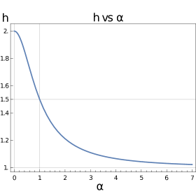
Figure 1: The dimension $h$ of operator (16) as a function of $\alpha$. $h$ approaches $1$ for $\alpha\rightarrow\infty$.

Before proceeding to the detailed investigation of this operator, let us discuss the possible symmetry breaking in this model. It is important because in the $\mathbb{Z}_{2}$ symmetry-broken phase the conformal solution (14) does not represent the thermodynamically dominating phase and the whole argument would not work. A closely related model, but with $\xi=0$, was studied by Kim–Klebanov–Tarnopolsky–Zhao(KKTZ) Kim:2019upg :

$$H_{\mathbb{Z}_{2}}=\frac{1}{4!}\sum_{ijkl}J_{ijkl}\left(\psi^{1}_{i}\psi^{1}_{j}\psi^{1}_{k}\psi^{1}_{l}+\psi^{2}_{i}\psi^{2}_{j}\psi^{2}_{k}\psi^{2}_{l}+6\alpha\psi^{1}_{i}\psi^{1}_{j}\psi^{2}_{k}\psi^{2}_{l}\right).$$ (18)

In fact, the above models have the same spectrum of conformal dimension in the antisymmetric $\psi^{1}\psi^{1}$, $\psi^{2}\psi^{2}$ bilinear sector. However the problem is that in the original KKTZ there is $\mathbb{Z}_{2}$ symmetry breaking for $|\alpha|>1$. Actual ground state is separated by a gap from the rest of the spectrum. At certain critical temperature $T_{crit}(\alpha)\sim N^{0}$ there is second-order phase transition. Below this temperature $\mathbb{Z}_{2}$ symmetry is broken and the actual physical behavior is not described by the conformal solution. However above $T_{crit}$ the physics is described by the conformal solution. Hence we expect that KKTZ model, once augmented with $\xi$-term, is also dominated by the non-local action, but only in some window of temperatures $T_{crit}(\alpha)<T\ll J$. Notice that after integrating out $J_{ijkl}$ in KKTZ model, SD equations contain mixed Green’s functions $G_{12},G_{21}$. The symmetry breaking is triggered by the operator

$$\mathcal{O}_{4}=\sum_{i}\psi^{1}_{i}\psi^{2}_{i}$$ (19)

in the symmetric sector which acquires complex scaling dimension for $|\alpha|>1$. In our case mixed correlators $G_{12}$ do not appear at all up to $1/N$ order. Therefore we conjecture that the symmetry breaking does not occur in our model and the non-local action dominates all the way to temperatures as low as $J/N^{1/(2h-2)}$. We verify this statement with finite $N$ exact diagonalization in Section 5.

2.2 A perturbative argument and thermodynamics

As we just found out, the coupled model does contain an operator with dimension $1<h<3/2$. Obviously, this irrelevant operator does not affect the conformal solution. How do we describe the influence of this operator on thermodynamics and other physical observables?

Let us review the arguments of SuhFirstPaper ; cft_breaking . In the standard SYK story(and in our coupled model) one obtains the conformal solution by neglecting the kinetic term in the SD equations. One way to recover the low energy physics is to consider conformal perturbation theory SuhFirstPaper (see Tikhanovskaya:2020elb ; Tikhanovskaya:2020zcw for a recent discussion). One starts from the artificial “exactly conformal” SYK without the kinetic term:

$$\mathcal{L}_{conf}=\sum_{ijkl}J_{ijkl}\psi_{i}\psi_{j}\psi_{k}\psi_{l}.$$ (20)

This theory taken literary is obviously pathological, as $\psi_{i}$ operators square to zero and lead to null states. However, the exact 2-functions are given by conformal solutions proportional to the one in eq. (14). We proceed by perturbing this theory by a set of irrelevant operators which are meant to mimic the kinetic term:

$$\mathcal{L}_{SYK}=\mathcal{L}_{conf}+\sum_{h}\alpha_{h}\mathcal{O}_{h}.$$ (21)

The most important operator in this sum is $h=2$ operator:

$$\mathcal{O}_{h=2}=\psi_{i}\partial_{u}\psi_{i}.$$ (22)

However, there are other terms with higher conformal dimensions. Notice that all of them come with unknown coefficients $\alpha_{h}$. Therefore one should be very careful in translating the operators in the UV Lagrangian to IR expansion in eq. (21). Specifically, we expect that in our case some $\alpha_{h}$ are non-linear in $\xi$.

Operator with $h=2$ gives rise to Schwarzian and has to be treated separately. We can try to treat other, $h\neq 2$ operators $\mathcal{O}_{h}$ in our model in a perturbative fashion. Naively, the leading contribution to the free energy comes from dressing the two-point function $\langle\mathcal{O}_{h}\mathcal{O}_{h}\rangle$ with reparametrizations:

$$\langle\mathcal{O}_{h}(u_{1})\mathcal{O}_{h}(u_{2})\rangle\propto\frac{1}{(u_{1}-u_{2})^{2h}}\rightarrow\left(\frac{\tau^{\prime}(u_{1})\tau^{\prime}(u_{2})}{(\tau(u_{1})-\tau(u_{2}))^{2}}\right)^{h}.$$ (23)

This leads to a non-local action for reparametrizations (2) with some unknown coefficient $\alpha_{2h}^{S}$. Crucially, the above computation assumes that 1-pt function $\langle\mathcal{O}_{h}\rangle$ vanishes.

Let us now describe elementary consequences of this. As long as temperatures are not too low, $T\gg J/N^{1/(2h-2)}$, the action (2) can be treated classically because of the overall factor of $N$. It is easy to check that the thermal solution is the same as in the Schwarzian case: $\tau(u)=\tan(\pi u/\beta)$. Plugging this solution into the Schwarzian action trivially yields the following free energy:

$$\Delta F_{Sch}/N=-\frac{2\pi^{2}\alpha_{Sch}^{S}}{J}T^{2}\rightarrow\Delta E_{Sch}/N=\frac{2\pi^{2}\alpha_{Sch}^{S}}{J}T^{2}.$$ (24)

The non-local action requires a bit more work. Assuming a fixed energy cutoff at $\sim J$, naive evaluation of the action yields a divergent term

$$-\beta\Delta F_{nonloc}/N=\frac{\alpha_{2h}^{S}}{J^{2h-2}}\beta^{2}\int_{0}^{1}d\widetilde{u}\ \left(\frac{\pi}{\beta\sin^{2}\left(\pi\widetilde{u}\right)}\right)^{2h}=\frac{\#}{T}+T^{2h-2}\frac{\alpha_{2h}^{S}\pi^{2h-1/2}}{J^{2h-2}}\frac{\Gamma\left(1/2-h\right)}{\Gamma\left(1-h\right)}.$$ (25)

Fortunately, this divergent term is proportional to $1/T$, hence it is simply a shift in the ground state energy cft_breaking . Throughout the paper we will be using the following notation for the free energy:

$$F/N=E_{0}/N-TS_{0}-f_{2h}T^{2h-1}-f_{Sch}T^{2}+\dots,$$ (26)

and energy:

$$E/N=E_{0}/N+c_{2h}T^{2h-1}+c_{Sch}T^{2}+\dots\ .$$ (27)

These coefficients are related by:

$$c_{Sch}=f_{Sch},\ c_{2h}=(2h-2)f_{2h}.$$ (28)

In this notation eq. (25) says that

$$f_{2h}=\frac{\alpha_{2h}^{S}\pi^{2h-1/2}}{J^{2h-2}}\frac{\Gamma\left(1/2-h\right)}{\Gamma\left(1-h\right)}.$$ (29)

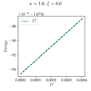
Figure 2: Energy vs $T^{2}$ for $J=2\pi$. Blue points are numerical data. For $\xi=0$ we expect Schwarzian answer.

We can easily check predictions from the Schwarzian and the non-local action against the numerical solution of SD equations. Using by now standard methods of solving SD equation in Euclidean time, we plotted energy versus temperature squared $T^{2}$. First consider the benchmark case with $\xi=0$ and $\alpha=1.8$ - Figure 2. Since $\xi=0$, we expect Schwarzian answer. We see that the energy is indeed proportional to $T^{2}$. We have performed this analysis for a wide range of $\beta$ between $50$ and $500$(not shown) and verified that the energy stays proportional to $T^{2}$. Now we switch to non-zero $\xi=0.5$ - Figure 3. We see a clear deviation from $T^{2}$ law. To quantify it, we have fitted the data with eq. (27) keeping $c_{Sch},c_{2h}$ and power $h$ unknown(i.e. they are extracted from the data). We see that $h_{best}$ are very close to theoretical values. Analysis at other values of $\alpha$(not shown) lead to similar results.

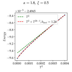
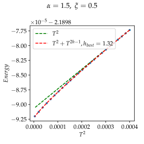
Figure 3: Energy vs $T^{2}$ for $J=2\pi$. Blue points are numerical data. We see a clear deviation from the Schwarzian prediction(dashed green is a straight line to guide the eye). For $\alpha=1.8$, $h_{theor}=1.24$ and for $\alpha=1.5$, $h_{theor}=1.31$. Changing the number of discretization points, temperature range and removing $c_{Sch}T^{2}$ term from the fit produces $h_{best}=1.24\pm 0.04$ for $\alpha=1.8$ and $h_{best}=1.32\pm 0.02$ for $\alpha=1.5$.

2.3 Twist $\xi$ dependence

As we have mentioned before, we do not really know $\xi$-dependence of coefficients $\alpha_{h}$ in the expansion (21). We addressed this question by numerically extracting coefficients $c_{2h}$ and $c_{Sch}$ in the energy, eq. (27) for different values of $\xi$. It is challenging to perform this computation because time discretization has to be smaller than the inverse $J_{eff}=J/(1-\xi)^{2}$, which becomes very big for $\xi\rightarrow 1$. This is why we plotted $c_{Sch},c_{2h}$ vs $\xi$ for different number of discretization points to make sure we converge. The results are presented in Figure 4.

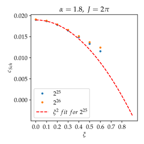
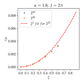
Figure 4: Coefficients $c_{Sch}$(Left) and $c_{2h}$(Right) versus $\xi$ for different number of discretization points $2^{25},2^{26}$.

We see that both $c_{Sch}$ and $c_{2h}$ start quadratic but then deviate from $\xi^{2}$ law. For large $\xi$ the dependence becomes slower than quadratic.

The Schwarzian coefficient $c_{Sch}$ decreases with $\xi$. From JT gravity perspective, adding $\xi$ terms introduces extra light matter in the bulk. We can try to compare this result to a similar problem: Schwarzian coupled to 2D CFT. This problem is exactly soluble Yang:2018gdb and CFT does lower Schwarzian coefficient.

3 Physics of non-local action

This Section is dedicated to various physical properties of the non-local action. Everywhere, except Section 3.5, we assume that $N$ is large and the temperatures are not too low($T\gg J/N^{1/(2h-2)}$) so that the non-local action can be treated classically. In Section 3.5 we compute leading $N^{0}$ correction to the free energy, which amounts to 1-loop computation. We do not perform any numerics here.

In many places we will need the form of quadratic fluctuations around the thermal solution. Expanding the non-local action (2) near the zero-temperature solution $\tau(u)=u+\epsilon(u)$ would yield

$$S_{nonloc,\beta=\infty}\propto\int dp\ \epsilon(p)|p|^{2h+1}\epsilon(-p).$$ (30)

However, we are interested in the finite temperature case $\tau(u)=\tan\left(\pi(u+\beta\epsilon(u))/\beta\right)$. In this case the fluctuations can be expanded in Fourier modes $\epsilon=\sum_{n}\epsilon_{n}e^{2\pi iun/\beta}$ giving rise to the following action

$$S_{nonloc,\beta}=\frac{N\alpha_{2h}^{S}m_{h}}{\left(\beta J\right)^{2h-2}}\sum_{n}\epsilon_{n}g_{h}(n)\epsilon_{-n},$$ (31)

with

$$g_{h}(n)=n^{2}\left(\frac{\Gamma(n+h)}{\Gamma(1+n-h)}-\frac{\Gamma(h-1)}{\Gamma(-h)}\right),$$ (32)

and numerical coefficient $m_{h}$ is

$$m_{h}=-(2\pi)^{2h+1}\frac{\pi(h-1)^{2}}{\cos(\pi h)\Gamma(2h)}.$$ (33)

For large $n$ we expect zero-temperature answer $g_{h}(n)\propto n^{2h+1}$. However even at small $n$ this is a good approximation. For bookkeeping, $\epsilon(u)$ and $\epsilon_{n}$ will always be dimensionless.

3.1 Residual entropy

For a warm-up, let us start from the zero-temperature entropy. Recall that the residual entropy at $T=0$ can be computed from evaluating $\operatorname*{Tr}\log G$ on the conformal solution parcollet1998 . In the model we are considering the conformal solution is exactly the same as in SYK model. Therefore the residual entropy is just twice Majorana SYK residual entropy:

$$S_{0}=2S_{0,SYK},$$ (34)

$$S_{0,SYK}=\int^{1/4}_{0}dx\ \frac{\pi x}{\tan(\pi x)}=0.2324\dots\ .$$ (35)

The actual residual entropy is $N$ times this, eq. (26). Our numerical results are consistent with this prediction.

3.2 Chaos exponent

In this Section we show that the non-local action (2) leads to a maximal chaos exponent Maldacena:2015waa in the out-of-time ordered correlation(OTOC) function.

The OTOC can be computed as follows. Since the reparametrizations is the only dominant physical mode at low energies, we need to dress the product of two 2-point functions with reparametrizations and average over them. In SYK one has to use the Schwarzian action (1), however in our case it is the non-local action (31). Leading $1/N$ contribution comes from using the linearized action (31):

$$\frac{\mathcal{F}}{G_{conf}(x)G_{conf}(x^{\prime})}=\frac{\langle\psi^{1}_{i}(\theta_{1})\psi^{1}_{i}(\theta_{2})\psi^{1}_{j}(\theta_{3})\psi^{1}_{j}(\theta_{4})\rangle_{conn}}{G_{conf}(x)G_{conf}(x^{\prime})}=$$

$$=\frac{(\beta J)^{2h-2}}{N}\frac{\pi^{2-2h}}{2m_{h}\alpha_{2h}^{S}}\sum_{|n|\geq 2}\frac{e^{in(y^{\prime}-y)}}{g_{h}(n)}\left[\frac{\sin\frac{nx}{2}}{\tan\frac{x}{2}}-n\cos\frac{nx}{2}\right]\left[\frac{\sin\frac{nx^{\prime}}{2}}{\tan\frac{x^{\prime}}{2}}-n\cos\frac{nx^{\prime}}{2}\right],$$ (36)

where $\theta_{i}$ are angle variables on the thermal circle $\theta=2\pi u/\beta$ and $y,y^{\prime},x,x^{\prime}$ are certain combinations of angles:

$$x=\theta_{1}-\theta_{2},\ x^{\prime}=\theta_{3}-\theta_{4},\ y=\frac{\theta_{1}+\theta_{2}}{2},\ y^{\prime}=\frac{\theta_{3}+\theta_{4}}{2}.$$ (37)

This piece dominates over contributions from other conformal fields due to $(\beta J)^{2h-2}$ enhancement.

In general this expression is complicated for ordering $\theta_{1}<\theta_{3}<\theta_{2}<\theta_{4}$ which is relevant for OTOC. Fortunately, it simplifies a lot when the points are antipodal on the circle. Specifically, we put

$$\theta_{1}=-\frac{\pi}{2}-\theta,\theta_{3}=0,\ \theta_{2}=\frac{\pi}{2}-\theta,\theta_{4}=\pi,$$ (38)

which corresponds to

$$x=x^{\prime}=-\pi,\ y=-\theta,y^{\prime}=\frac{\pi}{2}.$$ (39)

So we have

$$\sum_{|n|\geq 2}\frac{e^{in\left(\pi/2+\theta\right)}n^{2}\cos^{2}\frac{\pi n}{2}}{g_{h}(n)}.$$ (40)

We see that the sum goes over even $n$ only. We can convert the sum into the integral by introducing a factor $1/(e^{i\pi n}-1)$ and integrating over the contour $\mathcal{C}$ enclosing $\pm 2,\pm 4,\dots$:

$$\frac{1}{2}\oint_{\mathcal{C}}dn\ \frac{n^{2}}{e^{i\pi n}-1}\frac{e^{in\left(\pi/2+\theta\right)}}{g_{h}(n)}.$$ (41)

Now we can move the contour to infinity, since the integrand decays along the imaginary axis. It will pick up the pole at $n=0$ where $e^{i\pi n}=1$ and at locations where $g_{h}(n)$ has zeroes. The zeroes are located at $n=1,0,-1$ and at other negative $n$. Poles at negative $n$ are not relevant for us, because after analytically continuing to OTOC, namely $\theta\rightarrow-2\pi it/\beta$, they will produce exponentially decaying contributions(or a constant for $n=0$). The pole at $n=1$ yields maximal chaos exponent

$$\frac{\mathcal{F}(t)}{G_{conf}(\pi)G_{conf}(\pi)}=-p_{h}\frac{(\beta J)^{2h-2}}{N\alpha^{S}_{2h}m_{h}}\exp\left(\frac{2\pi t}{\beta}\right)+[\text{non-increasing}].$$ (42)

The fact that the chaos exponent is still maximal should not be too surprising: late time asymptotic growth $\sim e^{2\pi t/\beta}$ at late times $t\gg\beta$ can be found directly from the conformal solution KitaevTalks (and Section 3.6.1 of ms ) by computing the OTOC in the real time domain. However, the prefactor is parametrically smaller: for Schwarzian it is $(\beta J)^{1}$. It would be interesting to compute finite $\beta J$ corrections to the Lyapunov exponent and see that they satisfy the bound proposed in Zhang:2020jhn .

3.3 Time ordered 4-point function and energy-energy correlator

It is also interesting to consider time-ordered

$$\theta_{1}<\theta_{2}<\theta_{3}<\theta_{4},$$ (43)

4-point function. This computation will highlight a certain difference with SYK: in SYK $h=2$ mode(Schwarzian) is the energy operator, whereas in our case it is not.

We take the general expression (36) for the 4-point function and convert it into a contour integral:

$$\frac{(\beta J)^{2h-2}}{N\alpha^{S}_{2h}}\oint_{\mathcal{C}}dn\frac{1}{e^{2\pi in}-1}\frac{e^{in(y^{\prime}-y)}}{g_{h}(n)}\left[\frac{\sin\frac{nx}{2}}{\tan\frac{x}{2}}-n\cos\frac{nx}{2}\right]\left[\frac{\sin\frac{nx^{\prime}}{2}}{\tan\frac{x^{\prime}}{2}}-n\cos\frac{nx^{\prime}}{2}\right].$$ (44)

where the contour $\mathcal{C}$ encloses $\pm 2,\pm 3,\dots$. In the time-ordered case one can actually close the contour at infinity and pick up poles of $e^{2\pi in}-1$ and $g_{h}(n)$. In the usual SYK story, $g_{h}(n)\propto n^{2}(n^{2}-1)$ and the only contributing pole is at $n=0$. Because of this, the leading contribution to the 4-point function depends only on two variables $\theta_{1}-\theta_{2}$ and $\theta_{3}-\theta_{4}$($y,y^{\prime}$ drop out). Further taking the OPE limit $\theta_{1}\rightarrow\theta_{3},\ \theta_{3}\rightarrow\theta_{4}$ will produce the expression which is independent of $\theta_{i}$ at all. This is usually interpreted as follows: the OPE limit has produced the operator $\psi\partial_{\tau}\psi$ which is just the stress-energy operator $T$. Obviously, the correlator

$$\langle T(\theta_{1})T(\theta_{3})\rangle,$$ (45)

should not depend on $\theta_{1},\theta_{3}$ from the energy conservation. It turns out to be indeed the case. This allows one to compute the energy-energy correlators in SYK-chain models at any frequency $|\omega|\ll J$.

Let us return to our expression with complicated $g_{h}(n)$. Now we have to take into account poles of $g_{h}(n)$ at negative $n$. Because of that, the OPE limit $\theta_{1}\rightarrow\theta_{2},\ \theta_{3}\rightarrow\theta_{4}$ will produce an expression which is $\theta_{1}-\theta_{3}$ dependent. We are forced to conclude that $\psi\partial_{\tau}\psi$ is no longer proportional to energy. So we cannot extract energy-energy correlators easily.

However, we can still do it, but only in the hydrodynamic regime $|\omega|\ll 1/\beta\ll J$ Song_2017 . We consider a general time reparametrization (15) of the 2-point function. In the hydrodynamic regime we keep only the leading derivative of $\tau(u)$:

$$\tau(u)=u+\epsilon^{\prime}\beta u+\dots\ .$$ (46)

By looking at the form of conformal 2-point function, eq. (14), we see that $\epsilon^{\prime}$ simply rescales $\beta$:

$$\delta\beta=-\beta^{2}\epsilon^{\prime}\ .$$ (47)

Now we propagate this change into energy:

$$\delta E=-\beta^{2}\frac{dE}{d\beta}\epsilon^{\prime}\ .$$ (48)

This way we identify $\epsilon^{\prime}$ and $\delta E$. Hence, knowing the correlators of $\epsilon^{\prime}$ we can obtain the correlators of energy. Obviously, correlators of $\epsilon^{\prime}$ are governed by the non-local action.

One can cross-check this relation. First, from explicitly differentiating the partition function one has

$$\langle(\delta E)^{2}\rangle=-\frac{dE}{d\beta}.$$ (49)

This implies

$$\langle\epsilon^{\prime}\epsilon^{\prime}\rangle=\frac{4\pi^{2}n^{2}}{\beta^{2}}\langle\epsilon_{n}\epsilon_{-n}\rangle=-\frac{1}{\beta^{4}\frac{dE}{d\beta}}.$$ (50)

Now, using the explicit $\epsilon$ propagator (31) and the expression for the energy (25) one can indeed verify the above relation. The identification between $\epsilon^{\prime}$ and $\delta E$ will be very useful when we discuss the chain model.

3.4 Diffusion in chain models

We can also study a chain build from our model and study transport properties. The model we will consider is very similar to the ones discussed in the literature Gu2017Local ; Song_2017 ; Khveshchenko:2017mvj ; Khveshchenko:2020rai . It was previously shown that in SYK chain models thermal conductivity and electrical resistivity are linear in the temperature, similar to strange metals. Also, when the Schwarzian dominates, the diffusion constant is temperature-independent. In this Section we will show that once the non-local action becomes dominant, the thermal conductivity is still linear in the temperature. However, the diffusion constant becomes temperature dependent.

The model we consider is simply 1D array of independent dots:

$$\mathcal{L}_{T,chain}=\sum_{x}\mathcal{L}_{T,x},$$ (51)

where for each $x$ Lagrangian $\mathcal{L}_{T,x}$ is given by eq. (3). After integrating out the disorder we get a bunch of non-interacting models (12). To make them interact, we add a tight-binding(in $x$) random interaction:

$$\mathcal{L}_{int,chain}=\frac{1}{2!^{2}}\sum_{x,ijkl}\left(V^{1,x}_{ij;kl}\psi^{1}_{i,x}\psi^{1}_{j,x}\psi^{1}_{k,x+1}\psi^{1}_{l,x+1}+V^{2,x}_{ij;kl}\psi^{2}_{i,x}\psi^{2}_{j,x}\psi^{2}_{k,x+1}\psi^{2}_{l,x+1}\right),$$ (52)

where each $V^{1/2,x}_{ij;kl}$ is skew symmetric in $ij$ and $kl$:

$$V^{1/2,x}_{ij;kl}=-V^{1/2,x}_{ji;kl}=-V^{1/2,x}_{ij;lk},$$ (53)

but do not mix the two pairs $ij$ and $kl$. The full configuration is illustrated in Figure 5.

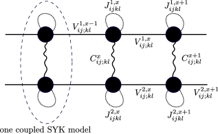
Figure 5: Illustration of couplings in the chain model.

Assuming $x-$independent variance

$$\langle\left(V^{1/2,x}_{ij;kl}\right)^{2}\rangle=\frac{V^{2}}{N^{3}},$$ (54)

we get the following extra terms in the $G\Sigma$-action:

$$\Delta S_{G\Sigma}=\frac{V^{2}}{8}\int du_{1}du_{2}\sum_{x}\left(G_{11,x}(u_{1},u_{2})^{2}G_{11,x+1}(u_{1},u_{2})^{2}+G_{22,x}(u_{1},u_{2})^{2}G_{22,x+1}(u_{1},u_{2})^{2}\right).$$ (55)

We have chosen the interaction term such that it does not lead to mixed $G_{12}$ correlators, which might cause instability. As usual, choosing $x-$independent ansatz for SD equations

$$G_{x,11}=G_{11},\quad G_{x,22}=G_{22},$$ (56)

we arrive at single-site SD equations (2.1) with effective $\widetilde{J}$ and $\widetilde{\alpha}$:

$$\widetilde{J}^{2}=J^{2}+V^{2},\quad\widetilde{\alpha}=\alpha\frac{J^{2}}{J^{2}+V^{2}}.$$ (57)

Now can discuss the kernel and the effective action for reparametrizations. We will assume that the reader is familiar with SYK 4-point function computation via ladder diagrams. This computation is pedagogically reviewed in Section 4.1 of this paper. We have two types of interactions in the chain model: on-site and between-site next-neighbor interaction, eq. (52). Performing a Fourier transform in the $x$ space makes the ladder diagrams(and the kernel) depend on momentum $p$. On-site interaction would produce $p$-independent part. Next-neighbor interaction will yield $\cos(p)$ dependence. So that the total kernel is

$$K_{chain}=K_{ren}+K_{p},$$ (58)

$K_{ren}$ is simply single-site kernel (107), but with renormalized $J,\alpha$:

$$K_{ren}v=\begin{pmatrix}3\widetilde{J}^{2}G_{11}*\left(\left(G_{11}^{2}+\widetilde{\alpha}^{2}G_{22}^{2}\right)v_{1}+\ 2\widetilde{\alpha}^{2}G_{11}G_{22}v_{2}\right)*G_{11}\\ 3\widetilde{J}^{2}G_{22}*\left(\left(G_{22}^{2}+\widetilde{\alpha}^{2}G_{11}^{2}\right)v_{2}+\ 2\widetilde{\alpha}^{2}G_{11}G_{22}v_{1}\right)*G_{22}\\ \end{pmatrix}$$ (59)

The remaining part is proportional to $\cos(p)-1$:

$$K_{p}v=2V^{2}(\cos(p)-1)\begin{pmatrix}G_{11}*(G_{11}^{2}v_{1})*G_{11}&0\\ 0&G_{22}*(G_{22}^{2}v_{2})*G_{22}\\ \end{pmatrix}$$ (60)

Note that $K_{p}$ is not proportional to $K_{ren}$. So in general it would be hard to find eigenvalues of $K_{chain}$. Fortunately, $K_{p}$ has the form of SYK kernel and in the leading conformal approximation $G_{11},G_{22}$ are proportional to the standard SYK conformal solution. So reparametrizations of $G$ again produce the kernel eigenvector with the eigenvalue close to $1$. In the small $p$ limit this is enough for us, since this term is proportional to $1-\cos(p)\approx p^{2}/2$.

Kernel $K_{ren}$ is analysed in Section 4.3 in detail. The upshot is that at $|\widetilde{\alpha}|>1$ its eigenvalue shift is controlled by the non-local action instead of the Schwarzian. Note that the conformal dimensions now are controlled by $\widetilde{\alpha}$, not $\alpha$. Putting this together we learn that the leading(in $1/\beta\widetilde{J}$ and $p$) eigenvalue shift for reparametrizations is

$$1-k(2,n,p)=\frac{\alpha^{K}_{2h}}{(\beta\widetilde{J})^{2h-2}}\frac{g_{h}(n)}{|n|(n^{2}-1)}+p^{2}\frac{V^{2}}{3\widetilde{J}^{2}(1+3\widetilde{\alpha}^{2})}.$$ (61)

So that the action for infinitesimal reparametrizations is given by

$$S=\frac{\pi^{4}b^{4}N}{4}\sum_{n,p}\epsilon_{n,p}\left(\frac{\alpha^{K}_{2h}}{(\beta\widetilde{J})^{2h-2}}g_{h}(n)+p^{2}|n|(n^{2}-1)\frac{V^{2}}{3\widetilde{J}^{2}(1+3\widetilde{\alpha}^{2})}\right)\epsilon_{-n,-p}.$$ (62)

One final step is to switch to Minkowski space and consider the limit of small time frequencies. Recall the analytic expression eq. (32) for $g_{h}(n)$. We need to continue $in\rightarrow\frac{\beta\omega}{2\pi}$ and consider the limit $\omega\rightarrow 0$ with fixed $\beta$. This way only the factor $n^{2}$ in $g_{h}(n)$ gives a finite contribution. Putting everything together we get:

$$S_{hydro}=\frac{\pi^{4}b^{4}N}{4}\frac{\beta}{2\pi}\int d\omega dp\ \epsilon_{\omega,p}\left(\frac{\alpha^{K}_{2h}}{(\beta\widetilde{J})^{2h-2}}\frac{(2h-1)\Gamma(h)}{\Gamma(2-h)}\frac{\omega^{2}\beta^{2}}{4\pi^{2}}+ip^{2}\frac{\omega\beta}{2\pi}\frac{V^{2}}{3\widetilde{J}^{2}(1+3\widetilde{\alpha}^{2})}\right)\epsilon_{-\omega,-p}.$$ (63)

Similarly to a single-site case, we identify $\partial_{t}\epsilon_{x}$ with energy at site $x$, eq. (48). We see a typical diffusion pole $\omega+iDp^{2}$ in the energy-energy correlator. The diffusion constant is given by

$$D=T^{3-2h}\frac{2\pi\Gamma(2-h)}{3(2h-1)\Gamma(h)}\frac{V^{2}\widetilde{J}^{2h-2}}{\alpha^{K}_{2h}\widetilde{J}^{2}(1+3\widetilde{\alpha}^{2})}.$$ (64)

A few comments are in order.

The important part is the temperature dependence $T^{3-2h}$. Schwarzian yields temperature-independent diffusion constant Gu2017Local ; Song_2017 . Here, the dimension $h$ of the irrelevant operator controls the temperature power.

Using the identification (48) between the energy and reparametrizations, one can also compute the energy-energy correlator and extract the thermal conductivity. It is proportional to the specific heat, eq. (27):

$$c_{v}=NT^{2h-2}(2h-2)(2h-1)\frac{\alpha_{2h}^{S}\pi^{2h-1/2}}{\widetilde{J}^{2h-2}}\frac{\Gamma\left(1/2-h\right)}{\Gamma\left(1-h\right)},$$ (65)

times the diffusion constant, eq. (64). Thus it is linear in the temperature as in the chains where Schwarzian dominate:

$$\kappa=c_{v}D\propto NT.$$ (66)

In the conventional SYK chain Gu2017Local the butterfly velocity is

$$v_{B}^{2}=2\pi DT,$$ (67)

which agrees with the holographic expectations Blake:2016wvh . However, careful computation of the butterfly velocity requires the knowledge of the subleading correction to the 4-point function Gu2017Local . In our case this seems complicated because the two kernels $K_{ren}$ and $K_{p}$ are not the same. Nonetheless, we conjecture that in our model the relation (67) still holds. Physically it is motivated by the fact that the same mode(reparametrizations) governs both OTOC chaos exponent and energy diffusion. This happens in the conventional SYK chains too. On the computational level, ignoring the subleading correction to 4-point function results in picking the pole at $\omega+iDp^{2}=0$, leading to eq. (67).

Unfortunately, we cannot study electric conductivity in our model because we do not have $U(1)$ symmetry. There are two ways to introduce $U(1)$ symmetry. We can simply promote the Majorana fermions to complex fermions. In this case one has to study operators in the symmetric sector which is not related to the Schwarzian. For example, in complex SYK KitaevRecent fluctuations in $U(1)$ phase are governed by simple $U(1)$-sigma model. However, there are also t-J models where resistivity is related to time reparametrization mode Guo_2020 . It would be interesting to see how the change from Schwarzian to non-local action affects the transport in t-J models. We leave this question for future work.

3.5 $N^{0}$ correction

In this Section we will compute $N^{0}$ correction to the free energy and try to infer the density of states $\rho(E)$ near the ground state. We would like to emphasize that in this Section we will be interested in the energies close to ground state: $|E-E_{0}|\sim N^{0}$. Whereas the thermodynamic results in eq. (25) corresponded to $|E-E_{0}|\sim N^{1}$. Also we will discuss below the validity of our $N^{0}$ computation.

We can easily compute $N^{0}$ correction to the free energy. Again, we will need some knowledge about the kernel eigenvalues so we refer to Sections 4.1 and 4.4 for the detailed discussion. The $N^{0}$ correction is given by the determinant of fluctuations around the thermal solution. Since reparametrizations are enhanced we expect that they will dominate in the determinant too. It can be argued diagramatically PS and by path-integral techniques ms that $N^{0}$ correction to $\log Z$ is given the sum of kernel eigenvalues

$$-\frac{1}{2}\sum_{h,n}\log\left(1-k(h,n)\right).$$ (68)

Obviously, the leading contribution will come from $k$ close to $1$, which are exactly reparametrizations.

As usual, let us start from the standard SYK case, where the Schwarzian dominates. Then the eigenvalue shift is proportional to, eq. (93):

$$\left(1-k(2,n)\right)_{Sch}\propto\frac{|n|}{\beta J},\quad|n|\geq 2.$$ (69)

The sum over $n$ has to be cut at $n\sim\beta J$. This produces the following answer:

$$\left(\log Z\right)_{Sch,1-loop}\propto\#\beta-\frac{3}{2}\log\left(\beta J\right).$$ (70)

The term proportional to $\beta$ has unknown coefficient, but it simply gives the shift to the ground state energy.

Let us discuss the non-local action now. From the linearized action (31), we expect the eigenvalue shift to be, eq. (119):

$$\left(1-k(2,n)\right)_{nonloc}\propto\frac{1}{(\beta J)^{2h-2}}\frac{g_{h}(n)}{|n|(n^{2}-1)}.$$ (71)

Recall that $g_{h}(n)$ is given by eq. (32). This sum is harder to evaluate. It can be simplified by noticing that one can separate the first term in the parenthesis:

$$g_{h}(n)=n^{2}\frac{\Gamma(n+h)}{\Gamma(1+n-h)}\eta_{h}(n),$$ (72)

with

$$\eta_{h}(n)=\left(1-\frac{\Gamma(h-1)\Gamma(1+n-h)}{\Gamma(-h)\Gamma(n+h)}\right).$$ (73)

We see that at large $n$, $\eta_{h}\propto 1-1/n^{2h-1}$ hence the sum $\sum_{|n|\geq 2}\log(\eta_{h})$ actually converges and gives something of order $(\beta J)^{0}$. We are not interested in this contribution. Now it is possible to evaluate the sum $\sum_{2\leq|n|\leq\beta J}\log\left(g_{h}(n)/(|n|(n^{2}-1)\eta_{h}(n))\right)$. The answer is

$$\left(\log Z\right)_{nonloc,1-loop}\propto\#\beta-\frac{3}{2}(2h-2)\log\left(\beta J\right).$$ (74)

We can try to convert this into the energy density by doing the inverse Laplace transform:

$$\rho(E)=\int d\beta\ Z(\beta)e^{-\beta E}.$$ (75)

In this equation the energy $E$ is measured from the ground state and it includes a factor of $N$. The most interesting regime, which actually can be probed with exact diagonalization, is the vicinity of the ground state, $E\sim N^{0}J$. However, one has to be extremely careful with the range of validity of (70) and (74). In this regime the above integral is dominated by $\beta\sim N/J$(in the Schwarzian case) and by $\beta\sim N^{1/(2h-2)}/J$(in the non-local case) and we cannot trust the above 1-loop computation anymore.

Fortunately for the Schwarzian, it is 1-loop exact Stanford:2017thb , so we can actually trust eq. (70) and obtain square-root edge:

$$\rho(E)_{Sch,1-loop}=\rho(E)_{Sch,exact}\propto\sqrt{E}.$$ (76)

Unfortunately, we do not know if the non-local action has the same property. Naively using 1-loop result (74) we get

$$\rho(E)_{nonloc,1-loop}\propto E^{3h-4}.$$ (77)

In fact, our exact diagonalization results at finite $N$ do not do not support this result. This suggests that the non-local action partition function is not 1-loop exact. We will discuss this more in Section 5.

4 Non-local action from 4-point function

This Section is entirely devoted to numerical, but ab initio 4-point function computation in our coupled model. One can look at this computation as the derivation of the non-local action. We will start by pedagogically reviewing the same computation in SYK. Then in Section 4.2 we discuss the leading non-conformal correction to 2-point functions. This Section can be read independently and the results are interesting on their own.

Schematically, the plan in this. In order to compute the 4-point function and identify the corresponding dominant low energy mode we need to:

• Write down ladder diagrams and find the corresponding kernel.

• Find the leading non-conformal correction to the 2-point function.

• Compute the kernel eigenvalue shift coming from this correction.

• Interpret the answer as an integral over reparametrizations with some action.

4.1 Review of Schwarzian derivation

Let us recall how Maldacena–Stanford(MS) ms argued that in SYK the low-energy physics is dominated by the Schwarzian action. Standard SYK has the following Hamiltonian:

$$H_{SYK}=\frac{1}{4!}\sum_{ijkl}J_{ijkl}\psi_{i}\psi_{j}\psi_{k}\psi_{l},\ \langle J_{ijkl}^{2}\rangle=\frac{3!J^{2}}{N^{3}}.$$ (78)

Summation of melonic diagrams lead to (Euclidean) Schwinger–Dyson equations for the two-point function $G(u_{1}-u_{2})\equiv G(12)=\langle T\psi_{i}(u_{1})\psi_{i}(u_{2})\rangle$:

$$(-i\omega_{n}-\Sigma(\omega_{n}))G(\omega_{n})=1,\ \omega_{n}=\frac{2\pi}{\beta}\left(n+\frac{1}{2}\right),$$ (79)

$$\Sigma(u)=J^{2}G(u)^{3}.$$ (80)

In the strict large $N$ these equations are exact. Compared to the rest of the paper, here the conformal solution differs by a factor of $\sqrt{1+3\alpha^{2}}$:

$$G_{conf}=b\operatorname*{sgn}(u)\frac{\pi}{\sqrt{J\beta\sin\left(\frac{\pi|u|}{\beta}\right)}},\ 1/J\ll|u|,\ \beta J\gg 1.$$ (81)

The (connected) 4-point function is given by the sum of ladder diagrams - Figure 6:

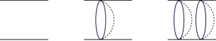
Figure 6: First few ladder diagrams contributing to the (connected) 4-point function. Solid lines are fermionic propagators and dashed lines indicate disorder contractions.

$$\langle\psi_{i}(\theta_{1})\psi_{i}(\theta_{2})\psi_{j}(\theta_{3})\psi_{j}(\theta_{4})\rangle=G(12)G(34)+\frac{1}{N}\mathcal{F},$$ (82)

$$\langle\psi_{i}(\theta_{1})\psi_{i}(\theta_{2})\psi_{j}(\theta_{3})\psi_{j}(\theta_{4})\rangle_{conn}=\frac{1}{N}\mathcal{F}(\theta_{1},\dots,\theta_{4})=\frac{1}{N}\frac{1}{1-K}\mathcal{F}_{0},$$ (83)

where $\mathcal{F}_{0}$ is the leading (connected) 4-point function:

$$\mathcal{F}_{0}(12;34)=-G(13)G(24)+G(14)G(23).$$ (84)

Explicitly the kernel $K=K(12;34)$ is given by

$$K(12;34)=-3J^{2}G(13)G(24)G(34)^{2}.$$ (85)

The kernel acts by convolution with the last two ($34$) variables. For example, the next-to-leading correction $\mathcal{F}_{1}$ is

$$\mathcal{F}_{1}(12;34)=K\mathcal{F}_{0}=\int d3^{\prime}d4^{\prime}K(12;3^{\prime}4^{\prime})\left[-G(3^{\prime}3)G(4^{\prime}4)+G(3^{\prime}4)G(4^{\prime}3)\right].$$ (86)

A natural thing to do is to expand $\mathcal{F}_{0}$ in the basis of eigenfunctions of $K$. Schematically:

$$\mathcal{F}=\sum_{k}\frac{1}{1-k}\frac{\langle\Psi_{k}|\mathcal{F}_{0}\rangle}{\langle\Psi_{k}|\Psi_{k}\rangle}\Psi_{k}.$$ (87)

It turns out, in the conformal limit $K$ has a set of eigenvalues equal to one: $k(2,n)=1$. The corresponding eigenfunctions are proportional to reparametrizations of $G$. The convenient basis of reparametrizations is

$$u\rightarrow u+\beta\sum_{n}\epsilon_{n}e^{-2\pi inu/\beta}.$$ (88)

They give enhanced contribution to the 4-point function

$$\text{(4-pt)}\supset\frac{1}{N}\frac{2}{\pi^{4}b^{4}}\sum_{n}\frac{1}{|n|(n^{2}-1)}\frac{k(2,n)}{1-k(2,n)}\delta_{\epsilon_{n}}G\ \delta_{\epsilon_{-n}}G,$$ (89)

with

$$\delta_{\epsilon_{n}}G(u_{1}-u_{2})=\pi G(u_{1}-u_{2})\left[\frac{\sin\frac{n\pi u}{\beta}}{\tan\frac{\pi u}{\beta}}-n\cos\frac{n\pi u}{\beta}\right]e^{i\pi n(u_{1}+u_{2})/\beta}.$$ (90)

The factor $2k(2,n)/(b^{4})$ came from the overlap between the $\mathcal{F}_{0}$ and the kernel eigenvector and $\pi^{4}|n|(n^{2}-1)$ came from the normalization of $\delta_{\epsilon_{n}}G$. The leading order answer can be obtained by taking the conformal answer everywhere except in $1-k(2,n)$. The difference $1-k(2,n)$ is determined by the leading non-conformal correction $\delta G$ to $G$. By analysing the large $q$ limit MS argued that the leading correction goes as $1/\beta J$:

$$\frac{\delta G}{G_{conf}}=-\frac{\alpha^{G}_{Sch}}{\beta J}f_{0}.$$ (91)

Function $f_{0}$ is given by

$$f_{0}=2+\frac{\pi-|\theta|}{\tan\frac{|\theta|}{2}},\quad\theta=2\pi u/\beta.$$ (92)

In the next sub-Section we will describe how to find these corrections in a systematic way.

From now on it is straightforward(but tedious) to find $1-k(2,n)$. MS did it analytically and found:

$$k(2,n)=1-\frac{\alpha^{K}_{Sch}|n|}{\beta J}.$$ (93)

Hence,

$$\text{(4-pt)}\supset\frac{1}{N}\frac{2\beta J}{\alpha^{K}_{Sch}\pi^{4}b^{4}}\ \sum_{n}\frac{1}{n^{2}(n^{2}-1)}\delta_{\epsilon_{n}}G\ \delta_{\epsilon_{-n}}G.$$ (94)

This answer can be understood as follows. We start from the leading (disconnected) contribution to the 4-point function, eq. (82):

$$G(u_{1}-u_{2})G(u_{3}-u_{4}),$$ (95)

where both Green functions are taken at finite (inverse) temperature $\beta$. Then we dress them with an infinitesimal reparametrization $u\rightarrow u+\beta\epsilon(u)$ and then average over $\epsilon$ with the action

$$S_{Sch}=\frac{N}{\beta J}8\pi^{4}\alpha^{S}_{Sch}\sum_{n}\epsilon_{n}n^{2}(n^{2}-1)\epsilon_{-n},\quad\alpha^{S}_{Sch}=\frac{\alpha^{K}_{Sch}b^{4}\pi^{4}}{32}.$$ (96)

Now, if we take the Schwarzian action

$$S=-\frac{N\alpha^{S}_{Sch}}{J}\int du\operatorname*{Sch}(\tau[u],u),$$ (97)

and expand it near the thermal solution:

$$\tau(u)=\tan\left(\frac{\pi}{\beta}\left(u+\beta\epsilon(u)\right)\right),$$ (98)

we get exactly the action (96). Hence the Schwarzian reproduces the correct answer for the 4-point function. Notice that it has the correct $n$ dependence and correct $\beta J$ dependence.

4.2 Correction to conformal solution

In the previous Section we promised to present a general approach for computing corrections to the conformal 2-point function. This approach is nothing more than a simple conformal perturbation theory associated with the deformation (21). For example Tikhanovskaya:2020elb ; Tikhanovskaya:2020zcw , the leading correction from an operator $\mathcal{O}_{h}$ of dimension $h$ is given by the 3-point function:

$$(\delta G)_{h}(u)=\alpha_{h}\int du^{\prime}\ \langle\mathcal{O}_{h}(u^{\prime})\psi_{i}(u)\psi_{i}(0)\rangle\propto\frac{1}{(Ju)^{h-1/2}}.$$ (99)

Answer $f_{h}=u^{1/2-h}$ is valid either at zero temperature or in the regime $1/J\ll|u|\ll\beta$. More generally, this correction is given by a hypergeometric function. In principle, one can compute even the second-order correction Tikhanovskaya:2020elb ; Tikhanovskaya:2020zcw :

$$(\delta^{2}G)_{h_{1}h_{2}}(u)=\alpha_{h_{1}}\alpha_{h_{2}}\int du_{1}du_{2}\ \langle\mathcal{O}_{h_{1}}(u_{1})\mathcal{O}_{h_{2}}(u_{2})\psi_{i}(u)\psi_{i}(0)\rangle\propto\frac{1}{(Ju)^{h_{1}+h_{2}-3/2}}.$$ (100)

Again, the final answer $f_{h_{1}+h_{2}}\propto 1/u^{h_{1}+h_{3}-3/2}$ is valid for $1/J\ll|u|\ll\beta$.

It can be shown that the leading correction in SYK(eq. (91)) comes from $h=2$ operator. However, we see right away that any operator with $h<2$(not necessarily $h<3/2$) will dominate over this $h=2$ correction. We would like to verify this statement in our coupled model.

Given the simplicity of $\beta=\infty$ answers, we will find the exact 2-point function numerically at zero temperature in Lorentzian time. The procedure is described in Appendix A. Specifically, we will examine the spectral density:

$$\rho_{11/22}=\operatorname{Im}G_{R,11/22}(\omega),$$ (101)

where $G_{R}$ is retarded 2-point function and $\omega$ is real frequency. From eqns. (99) and (100) $\rho$ has the following expansion:

$$\rho_{11/22}\times\sqrt{\omega}=\operatorname{const}+\sum_{h}A^{11/22}_{h}\omega^{h-1}+\sum_{h_{1},h_{2}}B^{11/22}_{h_{1}h_{2}}\omega^{h_{1}+h_{2}-2}+\dots.$$ (102)

We have multiplied $\rho$ by $\sqrt{\omega}$ because the leading conformal answer goes as $1/\sqrt{\omega}$. We will concentrate on the leading $\omega^{h-1}$ correction. We expect it to be $\xi$-odd. So it should have a different sign for $G_{11}$ and $G_{22}$. Our strategy is the following: find $\rho_{11/22}\sqrt{\omega}$ at a given $J$ and $\alpha$ and perform the fit with

$$b_{1}+b_{2}\omega^{h-1},$$ (103)

with unknown $b_{1},b_{2}$ in two ways: put $h=h_{theor}(\alpha)$ obtained from eq. (17) or allow $h$ to be inferred from the data. In other words, perform the fit with unknown $h$ and obtain $h_{best}$. The uncertainty in $h_{best}$ arises from changing the fitting interval in $\omega$. One important thing to notice is that $h_{best}$ tends to overestimate $h$ by about $0.05$ because we have omitted the subleading corrections.

• Schwarzian benchmark: $\alpha=0$

  Here for $\alpha=0$ the two systems decouple and for any $\xi$ we have two independent SYK. The result for $\alpha=\xi=0$ is presented in Figure 7. We indeed see that for small $\omega$ there is a linear term coming from $h=2$ mode:

  $$\rho_{11/22}\sqrt{\omega}=b_{1}+b_{2}\omega.$$ (104)

  

  Figure 7: Spectral density for original SYK. For comparison, we fitted using the theoretical value $h_{\rm theor}=2$ and arbitrary $h$. The fit was performed with $b_{1}+b_{2}\omega^{h-1}$.

• $|\alpha|>1$: Here operator $\mathcal{O}_{2,0}$, eq. (16), has the dimension in the interval $1<h<3/2$, as can be easily seen from eq. (17). The results for $G_{22}$ are presented in Figure 8. To make the graphs more expressive we have taken rather large $\xi=0.9$.

  

  

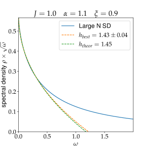
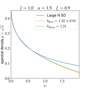
  Figure 8: Results for $G_{22}$, $\alpha>1$. The fit was performed with $b_{1}+b_{2}\omega^{h-1}$.

  Note that the leading correction has to be $\xi$-odd. Therefore we expect $\rho$ to curve in different directions for $G_{11}$. This is indeed the case as can be seen from Figure 9.

  

  

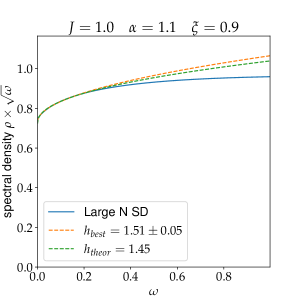
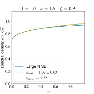
  Figure 9: Results for $G_{11}$, $|\alpha|>1$. The fit was performed with $b_{1}+b_{2}\omega^{h-1}$.

• $|\alpha|<1$: Now $\mathcal{O}_{2,0}$ has the dimension $3/2<h<2$. In this interval we do not expect the non-local action to dominate in the 4-point function or free energy. However, it still should dominate in the non-conformal correction. The results are presented in Figure 10. Again, to make the graphs more expressive we took rather large $\xi=0.9$.

  

  

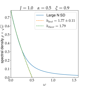
  Figure 10: Results for $G_{22}$, $|\alpha|<1$. The fit was performed with $b_{1}+b_{2}\omega^{h-1}$.

4.3 The kernel

Let us now discuss the kernel for our coupled model. In this Section we put $\beta=2\pi$. It is straightforward to draw ladder diagrams. However, the most convenient way to derive the kernel is to start from the conformal SD equations:

$$-J^{2}(G_{11}^{3}+3\alpha^{2}G_{11}G_{22}^{2})*G_{11}=\delta(u),$$

$$-J^{2}(G_{22}^{3}+3\alpha^{2}G_{22}G_{11}^{2})*G_{22}=\delta(u),$$ (105)

where $*$ means convolution in the Matsubara time domain, and perturb them by $G\rightarrow G+v$. The equations we obtain this way are

$$Kv=v,$$ (106)

where $K$ is the kernel and $v=(v_{1},v_{2})$ is the vector the kernel acts on. Explicitly we have

$$Kv=\begin{pmatrix}3J^{2}G_{11}*\left(\left(G_{11}^{2}+\alpha^{2}G_{22}^{2}\right)v_{1}+\ 2\alpha^{2}G_{11}G_{22}v_{2}\right)*G_{11}\\ 3J^{2}G_{22}*\left(\left(G_{22}^{2}+\alpha^{2}G_{11}^{2}\right)v_{2}+\ 2\alpha^{2}G_{11}G_{22}v_{1}\right)*G_{22}\\ \end{pmatrix}.$$ (107)

Correspondingly, the kernel is a $2\times 2$ matrix with four time variables:

$$K=K_{ab}\left(u_{1},u_{2};u_{3},u_{4}\right).$$ (108)

Four-point function $\mathcal{F}_{ab}$ is also a $2\times 2$ matrix corresponding to 4 different correlators:

$$\mathcal{F}_{ab}=\begin{pmatrix}\langle\psi^{1}\psi^{1}\psi^{1}\psi^{1}\rangle&\langle\psi^{1}\psi^{1}\psi^{2}\psi^{2}\rangle\\ \langle\psi^{2}\psi^{2}\psi^{1}\psi^{1}\rangle&\langle\psi^{2}\psi^{2}\psi^{2}\psi^{2}\rangle\end{pmatrix}.$$ (109)

We can write down the expression identical to eq. (87), which says that $\mathcal{F}\propto(1-K)^{-1}\mathcal{F}_{0}$. We will use the conformal solution everywhere except in $1-k$. This way the conformal kernel is proportional to SYK kernel:

$$K_{conf,ab}(12;34)=-3J^{2}G_{conf}(13)G_{conf}(24)G_{conf}(34)^{2}\begin{pmatrix}1+\alpha^{2}&2\alpha^{2}\\ 2\alpha^{2}&1+\alpha^{2}\end{pmatrix}.$$ (110)

Eigenvalue $1$ eigenvector $\Psi_{k=1}$ corresponds to reparametrizations. Because of non-zero $\alpha$, $G_{11}$ and $G_{22}$ have to be reparametrized the same way, so $\Psi_{k=1}$ has equal components:

$$\Psi_{k=1}\propto\begin{pmatrix}1\\ 1\\ \end{pmatrix}.$$ (111)

It is indeed easy to see that this vector is an eigenvector of the conformal kernel matrix in eq. (110). Because of this, the leading answers for all four 4-point functions in eq. (109) are going to be the same. Notice that the kernel does not contain $\xi$ explicitly, as it is determined by the ladder diagrams. The $\xi$ is actually present in the non-conformal correction to $G$ and hence in the eigenvalue shift $1-k(2,n)$. In the coupled model this correction is:

$$G_{exact,11/22}=G_{conf}+\delta G_{11/22}.$$ (112)

Let us discuss which of the terms in $\delta G$ contribute to the eigenvalue shift $k(2,n)_{conf}-k(2,n)_{exact}=1-k(2,n)_{exact}$. Since the conformal $G_{11/22}$ do not depend on $\xi$, eq. (14), they and the conformal kernel have $\mathbb{Z}_{2}$ symmetry $11\leftrightarrow 22$. In order to obtain the leading eigenvalue shift we need to compute $\langle\Psi_{k=1}|\delta K|\Psi_{k=1}\rangle$. The leading $(\beta J)^{h-1}$ correction to $G$ comes from computing the 3-pt function, eq. (99), where in our case the lightest operator is

$$\mathcal{O}_{h}=-\xi\sum_{i}\left(\psi^{1}_{i}\partial_{u}\psi^{1}_{i}-\psi^{2}_{i}\partial_{u}\psi^{2}_{i}\right).$$ (113)

Crucially, it is linear in $\xi$. In other words, it contributes with different signs to $\delta G_{11}$ and $\delta G_{22}$:

$$\frac{\delta G_{11}}{G_{conf}}=-\frac{\alpha^{G}_{h}}{\left(\beta J\right)^{h-1}}f_{h},$$ (114)

$$\frac{\delta G_{22}}{G_{conf}}=+\frac{\alpha^{G}_{h}}{\left(\beta J\right)^{h-1}}f_{h}.$$ (115)

Because of this asymmetry the leading correction from $f_{h}$, $\langle\Psi_{k=1}|\delta K|\Psi_{k=1}\rangle$ will vanish. Including the subleading correction (100) we have

$$\frac{\delta G_{11/22}}{G_{conf}}=\mp\frac{\alpha^{G}_{h}}{\left(\beta J\right)^{h-1}}f_{h}-\frac{\alpha^{G}_{2h}}{\left(\beta J\right)^{2h-2}}f_{h+h}-\frac{\alpha^{G}_{Sch}}{\beta J}f_{0}+\dots\ .$$ (116)

Therefore, the leading $\delta G$ correction $f_{h}$ can only contribute to $\delta k$ starting at quadratic order. However, it can mix with $f_{h+h}$: it is even in $\xi$, and hence can contribute to the eigenvalue shift in the leading order. This is why the analytic computation of the eigenvalue shift seems very difficult and we resort to numerics.

Note that because of the original $\mathbb{Z}_{2}$ symmetry at $\xi=0$, the one point function $\langle\mathcal{O}_{h}\rangle$ vanishes(in the first order of perturbation theory). So the absence of $(\beta J)^{h-1}$ term in the MSY computation and in the kernel computation has the same origin.

4.4 Eigenvalue shift

We will diagonalize the kernel and find the eigenvalues closest to $1$ following ref. KitaevRecent . It can be done numerically by introducing a 2D grid. We will fix $\beta=2\pi$ and study different $J$. Index $n$ arises by noticing that the kernel is invariant under translations and so $n$ is the momentum:

$$K_{n,ab}(u,u^{\prime})=\int_{0}^{2\pi}ds\ K_{ab}\left(s+\frac{u}{2},s-\frac{u}{2};\frac{u^{\prime}}{2},-\frac{u^{\prime}}{2}\right)e^{-ins}.$$ (117)

Since we are interested in the asymmetric kernel, it would be convenient to anti-symmetrize $u,u^{\prime}$ explicitly:

$$K^{A}_{n,ab}(u,u^{\prime})=\frac{1}{2}\left(K_{n,ab}(u,u^{\prime})-K_{n,ab}(u^{\prime},u)\right),$$ (118)

it improves the numerical results.

Let us start from a single SYK as a benchmark - Figure 11.

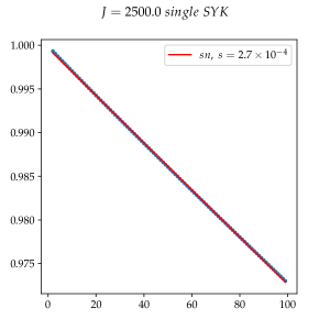
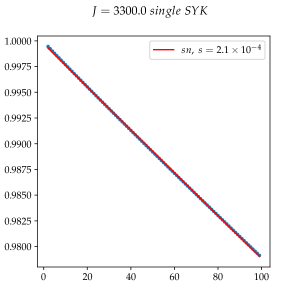
Figure 11: $k(2,n)$ versus $n$ plot for $J=2500$ and $J=3300$ single SYK. Red line is a linear fit to guide the eye.

We see a perfect agreement with the theoretical prediction $1-k(2,n)\propto n$.

Now we need to understand what kind of eigenvalue shift we expect from the non-local action. From the SYK discussion in Section 4.1 and eq. (31) it follows that the eigenvalue shift is determined by $g_{h}(n)/(|n|(n^{2}-1))$:

$$(1-k(2,n))_{nonloc}=\frac{\alpha^{K}_{2h}}{(\beta J)^{2h-2}}\frac{g_{h}(n)}{|n|(n^{2}-1)}.$$ (119)

Coefficients $\alpha^{K}_{2h}$ and $\alpha^{S}_{2h}$ are related by

$$\alpha^{K}_{2h}=\frac{4m_{h}}{\pi^{4}b^{4}}\alpha^{S}_{2h},$$ (120)

where $m_{h}$ is given by eq. (33). Therefore, at large $n$ we expect the following behavior:

$$\left(1-k(2,n)\right)_{nonloc}=\alpha_{2h}^{K}\frac{n^{2h-2}}{(\beta J)^{2h-2}}.$$ (121)

In fact, for our range of $h$, $g_{h}(n)$ is almost indistinguishable from a power-law except for the first few $n$. This motivates us to try to fit our results with a combination of a linear piece $n$(Schwarzian) and $n^{2h-2}$(non-local). For $h$ in the range $1<h<3/2$ the power $n^{2h-2}$ is less than $1$. It means that for large $n$ and $h$ not too close to $3/2$, the Schwarzian will dominate at large $n$. In order to check this we have plotted $k(2,n)$ for $n=2,\dots,100$ for various values of $J$ and $\alpha$.

Let us consider $\alpha=1.1$, $\alpha=1.5$ and $\alpha=1.8$ - Figures 12, 13, 14. All of them show non-linear behavior which turns into a linear one for large $n$ (left side in the plots). Presumably for large $n$ the Schwarzian piece starts to dominate. Naive log-log plot is not very instructive for two reasons: non-local contribution is not exactly a power-law and also we have a mixed expression with the linear Schwarzian contribution and the non-linear piece (121). Let us describe in detail Figures 12, 13, 14. We start from the left part, which is $k(2,n)$:

• Blue dots are numerically obtained $k(2,n)$.

• We could try to extract the linear term at large $n$ by fitting $k(2,n)$ with a line $sn$(red line), keeping $s$ unknown. However, it turned out that for our range of $\beta J$ the non-linear piece is still not negligible even at large $n\sim 100$.

• So in order to extract the linear piece properly we perform the fit with the non-linear piece (121) as well:

  $$1-\widetilde{s}n-\widetilde{A}n^{2h_{theor}-2},$$ (122)

  with unknown $\widetilde{s},\widetilde{A}$ and where $h_{theor}$ is the theoretical value of the scaling dimension. This is the orange curve. As we see from the plots, slope $\widetilde{s}$ is not close to naive slope $s$. This means that the nonlinear piece is indeed not negligible. We will use this slope $\widetilde{s}$ to subtract it from $k(2,n)$ and compare the result with the full non-local prediction $g_{h}(n)/(|n|(n^{2}-1))$.

• To double-check that we are not over-fitting by introducing to many parameters we perform a fit with unknown $\hat{s},\hat{A}$ and unknown power in the non-linear part:

  $$1-\hat{s}n-\hat{A}n^{2h-2}.$$ (123)

  This is green curve. In most cases it is indistinguishable from the orange one. The best value of $h=h_{best}$ is close to the theoretical $h_{theor}$. From using $2^{25}-2^{26}$ points for solving SD equation and $60,000^{2}-140,000^{2}$ 2D grid points for finding the kernel eigenvalues, we can estimate the uncertainty in $h_{best}$. We see that $h_{theor}$ and $h_{best}$ are within the uncertainty. As one can observe from the zero-temperature plots of the spectral function, Figures 8, 10, the numerics seem to overestimate $h$. We attribute the difference $h_{best}-h_{theor}$ to this systematic overestimation.

The right side is less intricate: we subtract $\widetilde{s}n$ from $k(2,n)$ and compare the result with the full non-local shift $g_{h}(n)/(|n|(n^{2}-1))$.

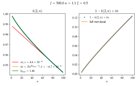
Figure 12: Results for $k(2,n)$. Details can be found in the main text. For $\alpha=1.1$, $h_{theor}=1.45$, whereas $h_{best}=1.46\pm 0.01$.

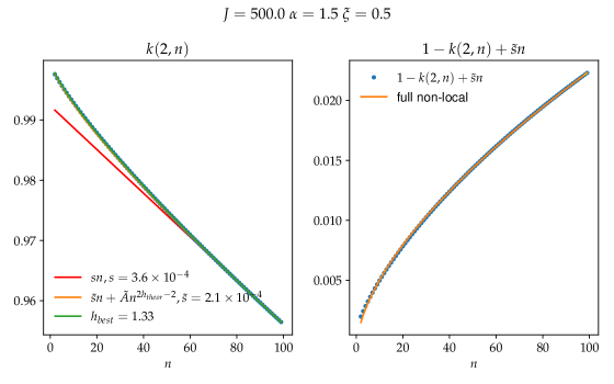
Figure 13: Results for $k(2,n)$. Details can be found in the main text. For $\alpha=1.5$, $h_{theor}=1.31$, whereas $h_{best}=1.35\pm 0.02$.

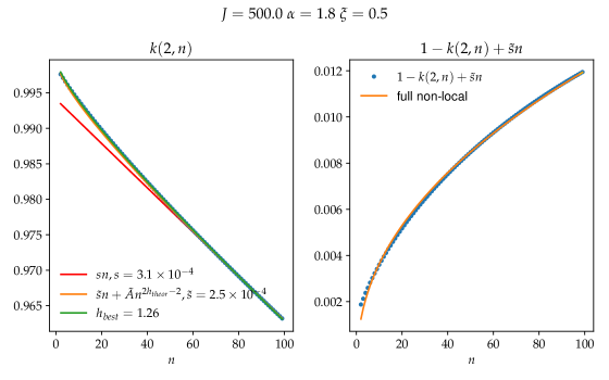
Figure 14: Results for $k(2,n)$. Details can be found in the main text. For $\alpha=1.8$, $h_{theor}=1.24$, whereas $h_{best}=1.28\pm 0.04$.

Finally, we can also check our results by considering $|\alpha|<1$. In this case we expect that the Schwarzian does dominate for large $\beta J$:

$$1-k(2,n)=\frac{\alpha_{Sch}^{K}|n|}{\beta J}+\frac{\alpha^{K}_{2h}}{\left(\beta J\right)^{2h-2}}|n|^{2h-2},n\gg 1,$$ (124)

where now $h>3/2$. It means that presumably at small $n$ the Schwarzian dominates and then for large $n$ the non-local piece starts to win. Moreover, from the analytic expression (32) we expect that $\alpha_{2h}^{K}$ is now negative, so $1-k(2,n)$ will still curve downwards. We considered $\alpha=0.5$ and again fitted $k(2,n)$ with eq. (124), keeping $h$ unknown - Figure 15. We again see a very good agreement with theoretical results.

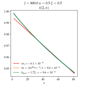
Figure 15: Results for $k(2,n)$. Details can be found in the main text. For $\alpha=0.5$, $h_{theor}=1.79$, whereas $h_{best}=1.72$.

4.5 Temperature dependence

Finally, the non-local action predicts that the non-linear term $n^{2h-2}$ in the eigenvalue shift behaves as $1/(\beta J)^{2h-2}$, eq. (121). The fitting strategy outlined in the previous Section allowed us to extract this coefficient. We considered $\alpha=1.1$ and $\alpha=1.5$ and plotted this coefficient for different $J$. After that, we fitted the result with

$$\frac{c}{J^{2h-2}},$$ (125)

keeping $c$ and $h$ unknown. The results are presented in Figure 16. We see that $h_{best}$ is again very close to the theoretical value. One can also check that the resulting $\alpha_{2h}^{K}$ agrees well with $c_{2h}$ in Figure 4. This computation requires using the conversions (120) and (29).

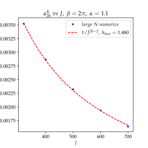
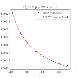
Figure 16: Coefficient $\alpha_{2h}^{K}$(here for convenience we included $\beta J$ inside $\alpha_{2h}^{K}$ compared to eq. (121)) as a function of $J$. Left: $\alpha=1.1$ for which $h_{theor}=1.45$. Right: $\alpha=1.5$ for which $h_{theor}=1.31$.

5 Exact diagonalization at finite $N$

One of the nice feature of SYK-like models in the opportunity to study finite-$N$ effects using exact diagonalization of the Hamiltonian. In our case the dimension of the Hilbert space is

$$\dim\mathcal{H}=2^{N},$$ (126)

so we can easily consider $N$ up to 16 without using any special techniques. Similar computations for the case of SYK has been done in the literature before ms , Bagrets2016Sachdev , GurAri2018Does , Kim:2019upg . We have performed finite $N$ exact diagonalization for four reasons:

• Cross-check our infinite $N$ solutions of SD equations.

• Probe the density of states near the ground state and see if it differs from the 1-loop result (77).

• See how the 2-point function behaves at very late times $\tau\gg N/J$.

• Check if the spectral correlators obey random matrix theory predictions. A deviation from them would indicate possible spin–glass phase at low temperatures GurAri2018Does .

As a starter we present the full spectrum binned with 300 bins for a single realization of disorder. Figure 17 shows the full spectrum of $N=32$ original Majorana SYK.

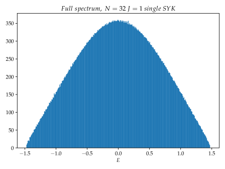
Figure 17: Full spectrum of $J=1,\ N=32$ single SYK for a single disorder realization binned with 300 bins.

Figure 18 shows the same quantity but for our coupled model with $\alpha=1.5,\ \xi=0.5$.

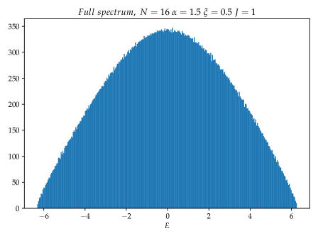
Figure 18: Full spectrum of $J=1,\ N=16,\ \alpha=1.5,\xi=0.5$ model for a single disorder realization binned with 300 bins.

We can also average over several samples to produce a more smooth density - Figure 19

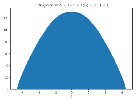
Figure 19: Full spectrum of $J=1,\ N=15,\ \alpha=1.5,\ \xi=0.5$ model averaged over 30 realization and binned with 300 bins.

The main takeaway from these plots is that the coupled model does not have a gap between the ground state and the rest of the spectrum. The presence of such gap would immediately imply that the conformal solution (14) does not represent the dominant thermodynamic solution.

5.1 Ground state energy

As we have mentioned in the Introduction, we are solving (Euclidean) SD equations (2.1) by the standard iteration procedure ms , when we start from a free solution $G_{11},G_{22}\propto\operatorname*{sgn}(u)$ and iterate the equations (2.1) until we converge(the norm between successive solutions becomes small). A natural question is: how do we know that we converge to an actual physical solution?

One way to check this is to compare the resulting ground state energy to the actual ground state energy computed from finite $N$ exact diagonalization. This requires two extrapolations. In SD we have to extrapolate finite-temperature energy all the way to $T=0$. This can be done using the prediction (27). In ED we have to extrapolate finite $N$ results to $N=\infty$. We can do this by assuming the following $N$ dependence in the ground state energy $E_{0}(N)$ at finite $N$:

$$E_{0}(N)=\left(E_{0}/N\right)N+c_{1}+c_{2}/N,$$ (127)

and extract $E_{0}/N,c_{1},c_{2}$ from the fit. The quantity $E_{0}/N\sim\mathcal{O}(N^{0})$ is supposed to match the result from SD.

As usual, we first present the result for $\xi=0$, which is supposed to have “conventional” Schwarzian physics - Figure 20. In Figure 21 we present the results for $\xi=0.5$ and different values of $\alpha$. In all cases we see a good agreement between SD and ED.

Figure 20: Finite $N$ exact diagonalization results for $\alpha=1.1,\xi=0.0,J=1.0$. The uncertainty comes from including a subleading term $c_{2}/N$ in the fit. Ground state energy from numerically solving large $N$ SD equations is $E_{0}/N=0.175(1)$.

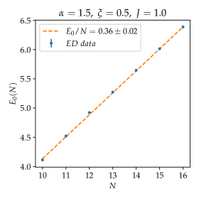
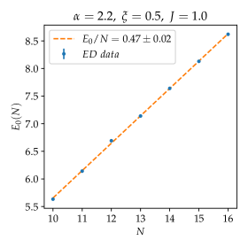
Figure 21: Finite $N$ exact diagonalization results for $\alpha=1.5$(Left) and $\alpha=2.2$(Right). For both cases $J=1.0,\xi=0.5$. The uncertainty comes from adding/removing a sub-subleading term $c_{2}/N$ in the fit. Ground state energy from numerically solving large $N$ SD equations is $E_{0}/N=0.351(3)$ for $\alpha=1.5$ and $E_{0}/N=0.466(1)$ for $\alpha=2.2$.

5.2 Density of states

It is very interesting to check the prediction (77) for the density of states:

$$\rho(E)_{non-loc,1-loop}\sim E^{3h-4}.$$ (128)

Famous Schwarzian result predicts Stanford:2017thb square-root edge $\sqrt{E}$ density of states near the ground state:

$$\rho(E)_{Sch,exact}\sim\sqrt{E}.$$ (129)

On ED side, working with the density of states directly is not good, because it depends on bin size. In order to eliminate this dependency we can plot ”cumulative distribution function”(CDF) which is just the number of states in a given energy interval from the ground state:

$$\text{CDF}(E)=\int_{E_{0}}^{E}\ dE^{\prime}\rho(E^{\prime}).$$ (130)

The results for the original SYK and the coupled model are shown in Figure 22.

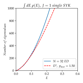
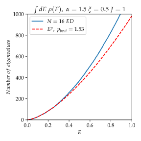
Figure 22: CDF for original $N=32$ SYK(Left) and coupled model with $N=16,\ \alpha=1.5,\xi=0.5$(Right). We have used a single realization of disorder. In both cases $J=1$. The power $p_{best}$ was determined from a fit with $AE^{p}$. $p_{best}$ obviously depends on the energy interval where the fit is performed. Changing this interval introduces $0.1$ uncertainty for SYK case and $0.07$ uncertainty for the coupled model.

We see a very good agreement with $\sqrt{E}$ for the case of original SYK. For $\alpha=1.5$, $h_{theor}=1.31$ so for the right part of Figure 22 the 1-loop result (128) predicts $E^{-0.07}$ which is definitely not the case. This indicates that the non-local action is not 1-loop exact. This numerical analysis suggests that the density of states keeps the square-root edge even when the Schwarzian is not dominant.

5.3 2-point function at very late times

Quantization of the Schwarzian action can be reduced to Liouville quantum mechanics Bagrets2016Sachdev ; mertens . At very late Euclidean times $\tau\gg N/J$ it results in a universal behavior $N/\tau^{3/2}$ in the 2-point function. In a single SYK, it is possible to see a power-law decay in ED even at moderate $N$. However one has to use large values of $N$ to see anything close to the power $3/2$. We would like to see what happens in the coupled model. Unfortunately, in the coupled model we are limited to $N=15$. Our results for a single SYK(for comparison) and the coupled model for $\alpha=1.5,\xi=0.5$ are presented in Figure 23. For this computation we did not use any approximations: we computed the full spectrum and wavefunctions by ED and then used them to determine the 2-point function at zero temperature by the spectral decomposition:

$$\langle 0|\psi_{i}(\tau)\psi_{i}(0)|0\rangle=\sum_{E_{n}}|\langle n|\psi_{i}|0\rangle|^{2}e^{-(E_{n}-E_{0})\tau}.$$ (131)

Finally, we averaged over 100 samples. We can confirm qualitative $1/\tau^{p}$ behavior, but we cannot reliable determine the power $p$. It seem to slowly increase with $N$. Our modest results suggest $p>1$. Presumably these results can be easily improved by studying larger $N$, but using low-lying states only.

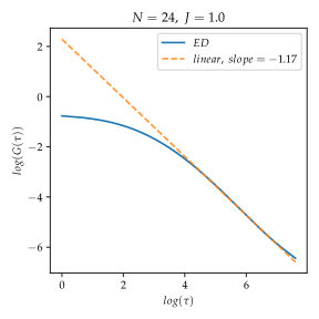
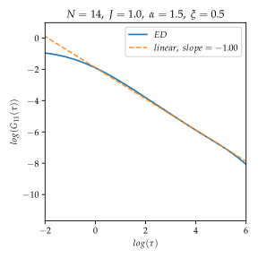
Figure 23: 2-point Green function at finite $N$ and large times. Left: original SYK. Right: the coupled model and $G_{11}$. Almost exactly the same results hold for $G_{22}$. In both cases we see a power-law behavior.

5.4 Level spacing

Another interesting quantity is the energy level statistics. A general expectation for chaotic models is that after making the energy density uniform, the energy gaps are distributed the same way as in a random matrix ensemble. A deviation from this indicate possible spin-glass phase GurAri2018Does . In this Section we are going to show that in the coupled model the level statistics obey random matrix theory predictions, suggesting no spin-glass phase. Compared to the rest of the paper, in this Section parameter $\xi$ is absorbed into $J^{1},J^{2},C$ couplings, making the fermionic operators square to one.

First of all, instead of unfolding the spectrum we consider another quantity: the ratio $r_{n}$ between the adjacent energy gaps:

$$r_{n}=\frac{E_{n+1}-E_{n}}{E_{n}-E_{n-1}}.$$ (132)

This quantity does not require unfolding. “Wigner-surmise”-like computation Atas_2013 predicts the following $r$ distribution:

$$P_{\beta}(r)=\frac{1}{Z_{\beta}}\frac{(r+r^{2})^{\beta}}{(1+r+r^{2})^{1+3\beta/2}},$$ (133)

where as usual $\beta=1$ correspond to Gaussian Orthogonal Ensemble(GOE), $\beta=2$ to Gaussian Unitary Ensemble(GUE) and $\beta=4$ to Gaussian Symplectic Ensemble(GSE). For comparison, for Poisson distributed levels the distribution is

$$P_{Poisson}(r)=\frac{1}{(1+r)^{2}}.$$ (134)

Now we need to understand what ensemble the coupled SYK Hamiltonian (8) corresponds to. Also we need to project out all global symmetries. The symmetry $\psi_{i}^{1}\leftrightarrow\psi_{i}^{2}$ is broken by $\xi$ term, so we should not worry about it. For even $N$ we have two independent and commuting symmetries: $\psi^{1}_{i}\rightarrow-\psi_{i}^{1}$, $\psi^{2}_{i}\rightarrow-\psi^{2}_{i}$. The corresponding operators are

$$\Gamma^{1}=i^{N/2}\prod_{i=1}^{N}\psi^{1}_{i},$$ (135)

$$\Gamma^{2}=i^{N/2}\prod_{i=1}^{N}\psi^{2}_{i}.$$ (136)

For odd $N$ only $\Gamma=\Gamma^{1}\Gamma^{2}$ is a symmetry. Having projected on eigenvalue subspace of these operators, we need to ask if we have any anti-linear symmetries. It is always possible to represent $\psi^{1}_{i}$ as real matrices and $\psi^{2}_{i}$ as purely imaginary matrices. Then there are three anti-linear symmetries:

$$K_{s}=\mathcal{C},$$ (137)

$$K_{1}=\left(\prod_{i=1}^{N}\psi_{i}^{1}\right)\mathcal{C},\quad K_{2}=\left(\prod_{i=1}^{N}\psi^{2}_{i}\right)\mathcal{C},$$ (138)

where $\mathcal{C}$ is complex-conjugation operator. They obey the following commutation relations for odd $N$:

$$K_{s}\Gamma=\Gamma K_{s},\quad K_{1,2}\Gamma=-\Gamma K_{1,2}.$$ (139)

Hence, for odd $N$ we have two sectors, $\Gamma=\pm 1$ and $K_{s}$ acts within them. Since $K_{s}^{2}=1$ we have GOE. Whereas for even $N$ the commutation relations are:

$$K_{s}\Gamma^{1,2}=(-1)^{N/2}\Gamma^{1,2}K_{s},$$ (140)

$$K_{1}\Gamma^{1,2}=(-1)^{N/2}\Gamma^{1,2}K_{1},\quad K_{2}\Gamma^{1,2}=(-1)^{N/2}\Gamma^{1,2}K_{2},$$ (141)

$$K_{s}^{2}=1,\quad\left(K_{1,2}\right)^{2}=(-1)^{N/2},$$ (142)

and there are four sectors: $\Gamma^{1,2}=\pm 1$. For even $N/2$, operators $K_{s,1,2}$ act within the sectors and we have GOE. For odd $N/2$ individual sectors do not have any anti-linear symmetries and the ensemble is GUE.

The numerical results are shown in Figure 24. We used 20 lowest eigenvalues after projecting out global symmetries. We see a perfect agreement with the surmise (133). This suggests the absence of spin-glass phase at low energies.

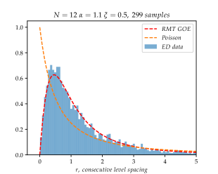
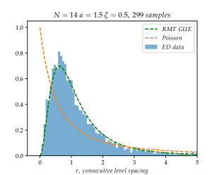
Figure 24: Distribution of $r$ for various $\alpha,\xi,N$. Random matrix prediction uses the surmise (133). For comparison, we included the exact result (134) for Poisson-distributed gaps.

6 Conclusion

In this paper we have presented a simple coupled SYK model. In the limit of large $N$ and low energies this model, like SYK, has an approximate time-reparametrization symmetry. However, unlike any previously known SYK-type model, the action for reparametrizations is dominated by a non-local action rather than the (local) Schwarzian. To verify this claim studied numerically different physical quantities, such as thermodynamic energy, subleading correction to 2-point function and 4-point function. Our approach was to solve large $N$ equations numerically. We saw that the non-local action indeed dominates everywhere. We double-checked some of our results using finite $N$ exact diagonalization.

Also we discussed other physical features of the coupled model and the non-local action. It turned out that the residual entropy and (maximal) chaos exponent are exactly the same as in SYK. However, the heat capacity and diffusion constant(in chain models) are very different from the models dominated by the Schwarzian. Also certain aspects of time-ordered 4-point function are different too. Also we presented a limited discussion of $1/N$ corrections. We computed the density of states near zero and saw that it does not agree with 1-loop prediction of the non-local action. This shows that the partition function is not 1-loop exact.

Let us comment on other models which can have an operator with dimension $1<h<3/2$ and thus exhibit the same physics. First of all, in the coupled model we have studied, apart from the operator (16), there is another set of operators which may have the dimension $1<h<3/2$, Kim:2019upg :

$$\mathcal{O}_{3,n}=\sum_{i}\left(\psi^{1}_{i}\partial_{u}^{2n+1}\psi^{2}_{i}+\psi^{2}_{i}\partial_{u}^{2n+1}\psi^{1}_{i}\right)$$ (143)

Their dimensions are determined by

$$\frac{2(\alpha+\alpha^{2})}{1+3\alpha^{2}}g_{A}(h)=1$$ (144)

Therefore the dimension of $\mathcal{O}_{3,0}$ can be in the window $(1,3/2)$ for $-1<\alpha<0$. However the operator $\mathcal{O}_{3,0}$ introduces non-diagonal(in $1,2$ indices) kinetic term. It can be diagonalized by a linear transformation of fermions, making it almost identical to the model we considered. We expect the physics to be the same as in our model. Two coupled SYK models(with 4-fermion interaction) admit another marginal interaction term:

$$\mathcal{L}^{\prime}_{int}=\sum_{ijkl}B^{1}_{i;jkl}\psi^{1}_{i}\psi^{2}_{j}\psi^{2}_{k}\psi^{2}_{l}+B^{2}_{ijk;l}\psi^{1}_{i}\psi^{1}_{j}\psi^{1}_{k}\psi^{2}_{l}$$ (145)

Compared to eq. (5) it couples 3 fermions from one side to 1 fermion from the other side. The resulting SD equations and the spectrum of conformal dimensions are very similar to the ones we studied. We again expect that in a certain range of parameters this model is dominated by the non-local action.

Let us conclude by a list of open questions:

• The most interesting question is to fully quantize the non-local theory (2). Is the Schwarzian piece important for this? Could it be that it starts dominating again in the strong-coupling region $\beta J\gg N$?

• Can we learn anything about JT gravity with matter from studying this model?

• Is there spin-glass phase? Our results about the level statistics suggest that there is no such phase.

• The model we described has an obvious generalization to $q$ interacting fermions.

• Unfortunately, we could not obtain much analytic progress in the large $q$ limit. Solving the model in this limit will give a partial analytical control over the models without the Schwarzian dominance.

• What is tensor-model counterpart? Some tensor models are different from SYK in $1/N$ corrections and they are not captured by the Schwarzian.

• What would be the physics of eternal traversable wormhole MQ ?

• What is the physics of the spectral form factor cotler2017black ?

• It would be instructive to incorporate complex fermions(or global symmetries in general) and study the interplay between them and the non-local action KitaevRecent . Models with complex fermions can have operators with dimensions $1<h<3/2$ too Klebanov:2020kck .

• Schwarzian term gives rise to the famous linear-temperature dependence of electrical resistivity in certain models Guo_2020 . It would be very interesting to generalize these models so that they are dominated by the non-local action. Presumably it will lead to a tunable temperature dependence in the resistivity.

• It would be interesting to investigate the dynamics of entanglement gu2017spread in the chain models.

• Finally, it is worth mentioning that in our model the point $|\alpha|=1$ seems to be special. At this value of $\alpha$ there is a field with $h=3/2$. However, because of $\cos(\pi h)$ in $m_{h}$, the 2-point function of reparametrizations (31) blows up.

Appendix A Lorentzian Schwinger–Dyson equations

Self-energies in Lorentzian signature are:

$$\Sigma^{>}_{11}=-\frac{1}{4}J^{2}\left(4(G^{>}_{11})^{3}+12\alpha^{2}G^{>}_{11}(G^{>}_{22})^{2}\right),$$

$$\Sigma^{>}_{22}=-\frac{1}{4}J^{2}\left(4(G^{>}_{22})^{3}+12\alpha^{2}G^{>}_{22}(G^{>}_{11})^{2}\right).$$ (146)

The relation between the self-energy and the retarded Green’s function is

$$G_{a}^{R}(\omega)=\frac{1}{(1-\xi_{a})\omega-\Sigma^{R}_{a}},\quad\xi_{11}=\xi,\xi_{22}=-\xi.$$ (147)

To close the system we need the fluctuation–dissipation theorem to relate $G^{>}$ to $G^{R}$:

$$G_{a}^{>}(\omega)=2in_{F}(\omega)\operatorname{Im}G_{a}^{R}(\omega),\quad n_{F}(\omega)=\frac{1}{e^{\beta\omega}+1},$$ (148)

Note that we can easily put $\beta=+\infty$. These equations can be solved by iterations, exactly like the Euclidean case. However one has to introduce a large interval in the time domain. So there will be two cut-offs: the time step $dt$ and the interval length $L$.

References

- (1) S. Sachdev and J. Ye, Gapless spin fluid ground state in a random, quantum Heisenberg magnet, Phys. Rev. Lett. 70 (1993) 3339 [cond-mat/9212030].
- (2) A. Kitaev, “A simple model of quantum holography.” http://online.kitp.ucsb.edu/online/entangled15/kitaev/,http://online.kitp.ucsb.edu/online/entangled15/kitaev2/.
- (3) D.J. Gross and V. Rosenhaus, A Generalization of Sachdev-Ye-Kitaev, 1610.01569.
- (4) O. Parcollet, A. Georges, G. Kotliar and A. Sengupta, Overscreened multichannel su(n) kondo model: Large-n solution and conformal field theory, Physical Review B 58 (1998) 3794–3813 [cond-mat/9711192].
- (5) A. Georges, O. Parcollet and S. Sachdev, Quantum fluctuations of a nearly critical Heisenberg spin glass, Physical Review B 63 (2001) 134406 [cond-mat/0009388].
- (6) R. Gurau, Colored Group Field Theory, Commun. Math. Phys. 304 (2011) 69 [0907.2582].
- (7) E. Witten, An SYK-Like Model Without Disorder, 1610.09758.
- (8) I.R. Klebanov and G. Tarnopolsky, Uncolored random tensors, melon diagrams, and the Sachdev-Ye-Kitaev models, Phys. Rev. D95 (2017) 046004 [1611.08915].
- (9) I.R. Klebanov and G. Tarnopolsky, On Large Limit of Symmetric Traceless Tensor Models, JHEP 10 (2017) 037 [1706.00839].
- (10) J. Maldacena, S.H. Shenker and D. Stanford, A bound on chaos, 1503.01409.
- (11) J. Maldacena and D. Stanford, Remarks on the Sachdev-Ye-Kitaev model, Phys. Rev. D94 (2016) 106002 [1604.07818].
- (12) A. Kitaev and S.J. Suh, The soft mode in the Sachdev-Ye-Kitaev model and its gravity dual, JHEP 05 (2018) 183 [1711.08467].
- (13) J. Maldacena and X.-L. Qi, Eternal traversable wormhole, 1804.00491.
- (14) W. Fu, D. Gaiotto, J. Maldacena and S. Sachdev, Supersymmetric SYK models, 1610.08917.
- (15) J.S. Cotler, G. Gur-Ari, M. Hanada, J. Polchinski, P. Saad, S.H. Shenker et al., Black Holes and Random Matrices, JHEP 05 (2017) 118 [1611.04650].
- (16) Y. Gu, A. Lucas and X.-L. Qi, Spread of entanglement in a sachdev-ye-kitaev chain, Journal of High Energy Physics 2017 (2017) .
- (17) J. Yoon, SYK Models and SYK-like Tensor Models with Global Symmetry, 1707.01740.
- (18) G. Gur-Ari, R. Mahajan and A. Vaezi, Does the syk model have a spin glass phase?, Journal of High Energy Physics 2018 (2018) .
- (19) J. Maldacena and A. Milekhin, SYK wormhole formation in real time, 1912.03276.
- (20) A. Almheiri, A. Milekhin and B. Swingle, Universal Constraints on Energy Flow and SYK Thermalization, 1912.04912.
- (21) Y. Chen, H. Zhai and P. Zhang, Tunable Quantum Chaos in the Sachdev-Ye-Kitaev Model Coupled to a Thermal Bath, JHEP 07 (2017) 150 [1705.09818].
- (22) P. Zhang, Evaporation dynamics of the Sachdev-Ye-Kitaev model, 1909.10637.
- (23) Y. Gu, A. Kitaev, S. Sachdev and G. Tarnopolsky, Notes on the complex Sachdev-Ye-Kitaev model, 1910.14099.
- (24) K. Su, P. Zhang and H. Zhai, Page curve from non-markovianity, 2101.11238.
- (25) J. Maldacena, D. Stanford and Z. Yang, Conformal symmetry and its breaking in two dimensional Nearly Anti-de-Sitter space, PTEP 2016 (2016) 12C104 [1606.01857].
- (26) F.M. Haehl and M. Rozali, Effective Field Theory for Chaotic CFTs, JHEP 10 (2018) 118 [1808.02898].
- (27) K. Nguyen, Reparametrization modes in 2d CFT and the effective theory of stress tensor exchanges, JHEP 21 (2020) 029 [2101.08800].
- (28) A. Milekhin, Coupled Sachdev-Ye-Kitaev models without Schwarzian dominance, 2102.06651.
- (29) Y. Gu, X.-L. Qi and D. Stanford, Local criticality, diffusion and chaos in generalized sachdev-ye-kitaev models, Journal of High Energy Physics 2017 (2017) 125 [1609.07832].
- (30) A. Altland, D. Bagrets and A. Kamenev, Quantum Criticality of Granular Sachdev-Ye-Kitaev Matter, Phys. Rev. Lett. 123 (2019) 106601 [1903.09491].
- (31) J. Kim, I.R. Klebanov, G. Tarnopolsky and W. Zhao, Symmetry Breaking in Coupled SYK or Tensor Models, Phys. Rev. X9 (2019) 021043 [1902.02287].
- (32) M. Tikhanovskaya, H. Guo, S. Sachdev and G. Tarnopolsky, Excitation spectra of quantum matter without quasiparticles I: Sachdev-Ye-Kitaev models, 2010.09742.
- (33) M. Tikhanovskaya, H. Guo, S. Sachdev and G. Tarnopolsky, Excitation spectra of quantum matter without quasiparticles II: random - models, Phys. Rev. B 103 (2021) 075142 [2012.14449].
- (34) Z. Yang, The Quantum Gravity Dynamics of Near Extremal Black Holes, JHEP 05 (2019) 205 [1809.08647].
- (35) P. Zhang, Y. Gu and A. Kitaev, An obstacle to sub-AdS holography for SYK-like models, 2012.01620.
- (36) X.-Y. Song, C.-M. Jian and L. Balents, Strongly correlated metal built from sachdev-ye-kitaev models, Physical Review Letters 119 (2017) [1705.00117].
- (37) D.V. Khveshchenko, Thickening and sickening the SYK model, SciPost Phys. 5 (2018) 012 [1705.03956].
- (38) D.V. Khveshchenko, Connecting the SYK Dots, Condens. Mat. 5 (2020) 37 [2004.06646].
- (39) M. Blake, Universal Charge Diffusion and the Butterfly Effect, 1603.08510.
- (40) H. Guo, Y. Gu and S. Sachdev, Linear in temperature resistivity in the limit of zero temperature from the time reparameterization soft mode, Annals of Physics 418 (2020) 168202 [2004.05182].
- (41) J. Polchinski and A. Streicher, unpublished , .
- (42) D. Stanford and E. Witten, Fermionic Localization of the Schwarzian Theory, JHEP 10 (2017) 008 [1703.04612].
- (43) D. Bagrets, A. Altland and A. Kamenev, Sachdev–Ye–Kitaev model as Liouville quantum mechanics, Nucl. Phys. B 911 (2016) 191 [1607.00694].
- (44) T.G. Mertens, G.J. Turiaci and H.L. Verlinde, Solving the Schwarzian via the Conformal Bootstrap, JHEP 08 (2017) 136 [1705.08408].
- (45) Y.Y. Atas, E. Bogomolny, O. Giraud and G. Roux, Distribution of the ratio of consecutive level spacings in random matrix ensembles, Physical Review Letters 110 (2013) [1212.5611].
- (46) I.R. Klebanov, A. Milekhin, G. Tarnopolsky and W. Zhao, Spontaneous Breaking of Symmetry in Coupled Complex SYK Models, JHEP 11 (2020) 162 [2006.07317].