Bayesian Quadrature on Riemannian Data Manifolds

Supplementary Material
Bayesian Quadrature on Riemannian Data Manifolds

Abstract

Riemannian manifolds provide a principled way to model nonlinear geometric structure inherent in data. A Riemannian metric on said manifolds determines geometry-aware shortest paths and provides the means to define statistical models accordingly. However, these operations are typically computationally demanding. To ease this computational burden, we advocate probabilistic numerical methods for Riemannian statistics. In particular, we focus on Bayesian quadrature (bq) to numerically compute integrals over normal laws on Riemannian manifolds learned from data. In this task, each function evaluation relies on the solution of an expensive initial value problem. We show that by leveraging both prior knowledge and an active exploration scheme, bq significantly reduces the number of required evaluations and thus outperforms Monte Carlo methods on a wide range of integration problems. As a concrete application, we highlight the merits of adopting Riemannian geometry with our proposed framework on a nonlinear dataset from molecular dynamics.

1 Introduction

The tacit assumption of a Euclidean geometry, implying that distances can be measured along straight lines, is inadequate when data follows a nonlinear trend, which is known as the manifold hypothesis. As a result, probability distributions based on a flat geometry may poorly model the data and fail to capture its underlying structure. Generalized distributions that account for curvature of the data space have been put forward to alleviate this issue. In particular, Pennec (2006) proposed an extension of the normal distribution on Riemannian manifolds such as the sphere.

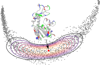
Figure 1: A land on a protein trajectory manifold of the enzyme adenylate kinase. Each datum represents a conformation of the protein, i.e., a spatial arrangement of its atoms. The conformation corresponding to the land mean ( ) is visualized.

The key strategy to use such distributions on general data manifolds is by replacing straight lines with continuous shortest paths, known as geodesics, which respect the nonlinear structure of the data. This is achieved by introducing a Riemannian metric in the data space that specifies how distance and volume are distorted locally.

To this end, Arvanitidis et al. (2016) proposed a maximum likelihood estimation scheme based on a data-induced metric to learn the parameters of a Locally Adaptive Normal Distribution (land), illustrated in Fig. 1. However, it relies on a computationally expensive optimization task that entails the repeated numerical integration of the unnormalized density on the manifold, for which no closed-form solution exists. Hence we are interested in techniques to improve the efficiency of the numerical integration scheme.

Probabilistic numerics (Hennig et al., 2015; Cockayne et al., 2019) frames computations that are subject to noise and approximation error as active inference. A probabilistic numerical routine treats the computer as a data source, acquiring evaluations according to a policy to decrease its uncertainty about the result. Amongst probabilistic numerical methods, we focus on Bayesian quadrature (bq) to compute intractable integrals on data manifolds. Bayesian quadrature (O’Hagan, 1991; Briol et al., 2019) treats numerical integration as an inference problem by constructing posterior measures over integrals given observations, i.e., evaluations of the integrand. Besides providing sound uncertainty estimates, the probabilistic approach permits the inclusion of prior knowledge about properties of the function to be integrated, and leverages active learning schemes for node selection as well as transfer learning schemes, for example when multiple similar integrals have to be jointly estimated (Xi et al., 2018; Gessner et al., 2019). These properties make bq especially relevant in settings where the integrand is expensive to evaluate, and make it a suitable tool for integration on Riemannian data manifolds.

Contributions

• The uptake of Riemannian methods in machine learning is principally hindered by prohibitive computational costs. We here address a key aspect of this bottleneck by improving the efficiency of integration on data manifolds.

• We customize Bayesian quadrature to curved spaces by exploiting knowledge about their structure. To this end, we introduce a tailored acquisition function that minimizes the number of expensive computations by selecting informative directions (instead of single points) on the manifold. Adopting a probabilistic numerical integration scheme enables efficient exploration of the integrand’s support under a suitable prior.

• We demonstrate accuracy and performance of our approach on synthetic and real-world data manifolds, where we observe speedups by factors of up to $20$. In these examples we focus on the land model, which provides a wide range of numerical integration problems of varying geometry and difficulty. We highlight molecular dynamics as a promising application area for Riemannian machine learning models. The results support the use of probabilistic numerical methods within Riemannian geometry to achieve significant speedup.

2 Riemannian Geometry

In our applied setting, we view $\mathbb{R}^{D}$ as a smooth manifold $\mathcal{M}$ with a changed notion of distance and volume measurement as compared to the Euclidean case. This view arises from the assumption that data have a general underlying nonlinear structure in $\mathbb{R}^{D}$ (see Fig. 2), and thus, the following discussion excludes manifolds with structure known a priori, e.g., spheres and tori. In our case, the tangent space $\mathcal{T}_{\boldsymbol{\mathsf{\mu}}}\mathcal{M}$ at a point $\boldsymbol{\mathsf{\mu}}\in\mathcal{M}$ is again $\mathbb{R}^{D}$, but centered at $\boldsymbol{\mathsf{\mu}}$. This is a vector space that allows to represent points of the manifold as tangent vectors $\boldsymbol{\mathsf{v}}\in\mathbb{R}^{D}$. Pictorially, a vector $\boldsymbol{\mathsf{v}}\in\mathcal{T}_{\boldsymbol{\mathsf{\mu}}}\mathcal{M}$ is tangential to some curve passing through $\boldsymbol{\mathsf{\mu}}$. Together, these vectors give a linearized view of the manifold with respect to a base point $\boldsymbol{\mathsf{\mu}}$. A Riemannian metric is a positive definite matrix $\boldsymbol{\mathsf{M}}:\mathbb{R}^{D}\rightarrow\mathbb{R}_{+}^{D\times D}$ that varies smoothly across the manifold. Therefore, we can define a local inner product between tangent vectors $\boldsymbol{\mathsf{v}},\boldsymbol{\mathsf{w}}\in\mathcal{T}_{\boldsymbol{\mathsf{\mu}}}\mathcal{M}$ as $\langle\boldsymbol{\mathsf{v}},\boldsymbol{\mathsf{w}}\rangle_{\boldsymbol{\mathsf{\mu}}}=\langle\boldsymbol{\mathsf{v}},\boldsymbol{\mathsf{M}}(\boldsymbol{\mathsf{\mu}})\boldsymbol{\mathsf{w}}\rangle$, where $\langle\cdot,\cdot\rangle$ is the Euclidean inner product. This inner product makes the smooth manifold a Riemannian manifold (do Carmo, 1992; Lee, 2018).

\begin{overpic}[width=199.4681pt]{fig/volume_element_explained_boxes.png} \put(3.0,3.0){\large$\displaystyle\mathcal{M}$} \put(68.5,58.0){\large$\displaystyle\operatorname{Exp}_{\boldsymbol{\mathsf{\mu}}}(\boldsymbol{\mathsf{v}})=\boldsymbol{\mathsf{x}}$} \put(66.0,15.0){\rotatebox{10.0}{\large$\displaystyle\operatorname{Log}_{\boldsymbol{\mathsf{\mu}}}(\boldsymbol{\mathsf{x}})=\boldsymbol{\mathsf{v}}$}} \end{overpic}

Figure 2: A protein trajectory manifold. A subset of the geodesics is shown with respect to a fixed point $\boldsymbol{\mathsf{\mu}}$ ( ). The background is colored according to the volume element $\sqrt{\lvert\boldsymbol{\mathsf{M}}\rvert}$ (Sec. 2.1) on a log scale. We omit a colorbar, since the values are not easily interpreted. Darker color indicates regions with small metric, to which shortest paths are attracted. For one geodesic ( ), we show the downscaled tangent vector and the $\operatorname{Log}$ and $\operatorname{Exp}$ operations.

A Riemannian metric locally scales the infinitesimal distances and volume. Consider a curve $\boldsymbol{\mathsf{\gamma}}:[0,1]\rightarrow\mathcal{M}$ with $\boldsymbol{\mathsf{\gamma}}(0)=\boldsymbol{\mathsf{\mu}}$ and $\boldsymbol{\mathsf{\gamma}}(1)=\boldsymbol{\mathsf{x}}$. The length of this curve on the Riemannian manifold $\mathcal{M}$ is computed as

$$L(\boldsymbol{\mathsf{\gamma}})=\int_{0}^{1}\sqrt{\langle\dot{\boldsymbol{\mathsf{\gamma}}}(t),\boldsymbol{\mathsf{M}}(\boldsymbol{\mathsf{\gamma}}(t))\dot{\boldsymbol{\mathsf{\gamma}}}(t)\rangle}\,\operatorname{d}\!t,$$ (1)

where $\dot{\boldsymbol{\mathsf{\gamma}}}(t)=\frac{\,\operatorname{d}\!}{\,\operatorname{d}\!t}\boldsymbol{\mathsf{\gamma}}(t)\in\mathcal{T}_{\boldsymbol{\mathsf{\gamma}}(t)}\mathcal{M}$ is the velocity of the curve. The $\boldsymbol{\mathsf{\gamma}}^{*}$ that minimizes this functional is the shortest path between the points. To overcome the invariance of $L$ under reparametrization of $\boldsymbol{\mathsf{\gamma}}$, shortest paths can equivalently be defined as minimizers of the energy functional. This enables application of the Euler-Lagrange equations, which result in a system of $2^{\text{nd}}$ order nonlinear ordinary differential equations (odes). The shortest path is obtained by solving this system as a boundary value problem (bvp) with boundary conditions $\boldsymbol{\mathsf{\gamma}}(0)=\boldsymbol{\mathsf{\mu}}$ and $\boldsymbol{\mathsf{\gamma}}(1)=\boldsymbol{\mathsf{x}}$. Such a length-minimizing curve is known as geodesic.

To perform computations on $\mathcal{M}$ we introduce two operators. The first is the logarithmic map $\operatorname{Log}_{\boldsymbol{\mathsf{\mu}}}(\boldsymbol{\mathsf{x}})=\boldsymbol{\mathsf{v}}$, which represents a point $\boldsymbol{\mathsf{x}}\in\mathcal{M}$ as a tangent vector $\boldsymbol{\mathsf{v}}\in\mathcal{T}_{\boldsymbol{\mathsf{\mu}}}\mathcal{M}$. This can be seen as the initial velocity of the geodesic that reaches $\boldsymbol{\mathsf{x}}$ at $t=1$ with starting point $\boldsymbol{\mathsf{\mu}}$. The inverse operator is the exponential map $\operatorname{Exp}_{\boldsymbol{\mathsf{\mu}}}(t\cdot\boldsymbol{\mathsf{v}})=\boldsymbol{\mathsf{\gamma}}(t)$ that takes an initial velocity $\dot{\boldsymbol{\mathsf{\gamma}}}(0)=\boldsymbol{\mathsf{v}}\in\mathcal{T}_{\boldsymbol{\mathsf{\mu}}}\mathcal{M}$ and generates a unique geodesic with $\boldsymbol{\mathsf{\gamma}}(0)=\boldsymbol{\mathsf{\mu}}$ and $\boldsymbol{\mathsf{\gamma}}(1)=\boldsymbol{\mathsf{x}}$. Note that $\operatorname{Log}_{\boldsymbol{\mathsf{\mu}}}(\operatorname{Exp}_{\boldsymbol{\mathsf{\mu}}}(\boldsymbol{\mathsf{v}}))=\boldsymbol{\mathsf{v}}$, and also, $\|\operatorname{Log}_{\boldsymbol{\mathsf{\mu}}}(\boldsymbol{\mathsf{x}})\|_{2}=\|\boldsymbol{\mathsf{v}}\|_{2}=L(\boldsymbol{\mathsf{\gamma}})$. Computationally, the logarithmic map amounts to solving a bvp, whereas the exponential map corresponds to an initial value problem (ivp). For general data manifolds, analytic solutions of the geodesic equations do not exist, so we rely on specialized approximate numerical solvers for the bvps; however, finding shortest paths still remains a computationally expensive problem (Hennig & Hauberg, 2014; Arvanitidis et al., 2019b). In contrast, the exponential map as an ivp is an easier problem and solutions are significantly more efficient.

We illustrate our applied manifold setting in Fig. 2, where we show geodesics starting from a point $\boldsymbol{\mathsf{\mu}}$, as well as the $\operatorname{Log}$ and $\operatorname{Exp}$ operators between $\boldsymbol{\mathsf{\mu}}$ and a point $\boldsymbol{\mathsf{x}}$. Note that Figs. 1 to 4 are in correspondence, that is, they illustrate different aspects of the same setting. More details on Riemannian geometry and the ode system are in A.1.

2.1 Constructing Riemannian Manifolds from Data

The Riemannian volume element or measure $\,\operatorname{d}\!\mathcal{M}(\boldsymbol{\mathsf{x}})=\sqrt{\lvert\boldsymbol{\mathsf{M}}(\boldsymbol{\mathsf{x}})\rvert}\,\operatorname{d}\!\boldsymbol{\mathsf{x}}$ represents the distorted infinitesimal standard Lebesgue measure $\,\operatorname{d}\!\boldsymbol{\mathsf{x}}$. For a meaningful metric, this quantity is small near the data and increases as we move away from them. Intuitively, this metric behavior pulls shortest paths near the data.

There are broadly two unsupervised approaches to learn such an adaptive metric from data. Given a dataset $\boldsymbol{\mathsf{x}}_{1:N}$ of $N$ points in $\mathbb{R}^{D}$, Arvanitidis et al. (2016) proposed a nonparametric metric to model nonlinear data trends as the inverse of a local diagonal covariance matrix with entries

$$M_{dd}(\boldsymbol{\mathsf{x}})=\left(\sum_{n=1}^{N}w_{n}(\boldsymbol{\mathsf{x}})(x_{nd}-x_{d})^{2}+\rho\right)^{-1},$$ (2)

where the weights $w_{n}$ are obtained from an isotropic Gaussian kernel $w_{n}(\boldsymbol{\mathsf{x}})=\exp\left(-\frac{||\boldsymbol{\mathsf{x}}_{n}-\boldsymbol{\mathsf{x}}||^{2}}{2\sigma^{2}}\right)$. The lengthscale $\sigma$ determines the curvature of the manifold, i.e., how fast the metric changes. The hyperparameter $\rho$ controls the value of the metric components that is reached far from the data, so the measure there is $\sqrt{\boldsymbol{\mathsf{\lvert M\rvert}}}=\rho^{-\frac{D}{2}}$. Typically, $\rho$ is set to a small scalar to encourage geodesics to follow the data trend. However, this metric does not scale to higher dimensions due to the curse of dimensionality (Bishop, 2006, Ch. 1.4).

Another approach relies on generative models to capture the geometry of high-dimensional data in a low-dimensional latent space (Tosi et al., 2014; Arvanitidis et al., 2018). Let a dataset $\boldsymbol{\mathsf{y}}_{1:N}~{}\in~{}\mathbb{R}^{D^{\prime}}$ with latent representation $\boldsymbol{\mathsf{x}}_{1:N}~{}\in~{}\mathbb{R}^{D}$ and $D^{\prime}>D$, such that $\boldsymbol{\mathsf{y}}_{n}\approx\boldsymbol{\mathsf{g}}(\boldsymbol{\mathsf{x}}_{n})$ where $\boldsymbol{\mathsf{g}}$ is a stochastic function with Jacobian $\boldsymbol{\mathsf{J}}_{\boldsymbol{\mathsf{g}}}(\boldsymbol{\mathsf{x}})\in\mathbb{R}^{D^{\prime}\times D}$. Then, the pullback metric $\boldsymbol{\mathsf{M}}(\boldsymbol{\mathsf{x}})=\mathbb{E}[\boldsymbol{\mathsf{J}}^{\intercal}_{\boldsymbol{\mathsf{g}}}(\boldsymbol{\mathsf{x}})\boldsymbol{\mathsf{J}}_{\boldsymbol{\mathsf{g}}}(\boldsymbol{\mathsf{x}})]$ is naturally induced in $\mathbb{R}^{D}$, which enables the computation of lengths that respect the geometry of the data manifold in $\mathbb{R}^{D^{\prime}}$. Even though this metric reduces the dimensionality of the problem and can be learned directly from the data by learning $\boldsymbol{\mathsf{g}}$, it is computationally expensive to use due to the Jacobian.

To mitigate this shortcoming, we propose a surrogate Riemannian metric. Consider a Variational Auto-Encoder (vae) (Kingma & Welling, 2014; Rezende et al., 2014) with encoder $q_{\phi}(\boldsymbol{\mathsf{x}}|\boldsymbol{\mathsf{y}})=\mathcal{N}(\boldsymbol{\mathsf{x}}~{}|~{}\boldsymbol{\mathsf{\mu}}_{\phi}(\boldsymbol{\mathsf{y}}),\operatorname{diag}(\boldsymbol{\mathsf{\sigma}}^{2}_{\phi}(\boldsymbol{\mathsf{y}})))$, decoder $p_{\theta}(\boldsymbol{\mathsf{y}}|\boldsymbol{\mathsf{x}})=\mathcal{N}(\boldsymbol{\mathsf{y}}~{}|~{}\boldsymbol{\mathsf{\mu}}_{\theta}(\boldsymbol{\mathsf{x}}),\operatorname{diag}(\boldsymbol{\mathsf{\sigma}}^{2}_{\theta}(\boldsymbol{\mathsf{x}})))$ and prior $p(\boldsymbol{\mathsf{x}})=\mathcal{N}(\boldsymbol{\mathsf{x}}~{}|~{}\boldsymbol{\mathsf{0}},\mathbb{I}_{D})$, with deep neural networks as the functions that parametrize the distributions. Then, the aggregated posterior is

$$q_{\phi}(\boldsymbol{\mathsf{x}})=\int_{\mathbb{R}^{D^{\prime}}}q_{\phi}(\boldsymbol{\mathsf{x}}~{}|~{}\boldsymbol{\mathsf{y}})p(\boldsymbol{\mathsf{y}})\,\operatorname{d}\!\boldsymbol{\mathsf{y}}\approx\frac{1}{N}\sum_{n=1}^{N}q_{\phi}(\boldsymbol{\mathsf{x}}~{}|~{}\boldsymbol{\mathsf{y}}_{n}),$$ (3)

where the integral is approximated from the training data. This is a Gaussian mixture model that assigns non-zero density only near the latent codes of the data. Thus, motivated by Arvanitidis et al. (2020) we define a diagonal Riemannian metric in the latent space as

$$\boldsymbol{\mathsf{M}}(\boldsymbol{\mathsf{x}})=(q_{\phi}(\boldsymbol{\mathsf{x}})+\rho)^{-\frac{2}{D}}\cdot\mathbb{I}_{D}.$$ (4)

This metric fulfills the desideratum of modeling the local behavior of the data in the latent space and it is more efficient than the pullback metric. The variance $\sigma^{2}_{\phi}(\cdot)$ of the components is typically small, so the metric adapts well to the data, which, however, may result in high curvature.

3 Gaussians on Riemannian Manifolds

Pennec (2006) theoretically derived the Riemannian normal distribution as the maximum entropy distribution on a manifold $\mathcal{M}$, given a mean $\boldsymbol{\mathsf{\mu}}$ and covariance matrix $\boldsymbol{\mathsf{\Sigma}}$. The density on $\mathcal{M}$ is

$$p(\boldsymbol{\mathsf{x}})=\frac{1}{\mathcal{C}(\boldsymbol{\mathsf{\mu}},\boldsymbol{\mathsf{\Sigma}})}\exp\left(-\frac{1}{2}\left\langle\operatorname{Log}_{\boldsymbol{\mathsf{\mu}}}(\boldsymbol{\mathsf{x}}),\boldsymbol{\mathsf{\Sigma}}^{-1}\operatorname{Log}_{\boldsymbol{\mathsf{\mu}}}(\boldsymbol{\mathsf{x}})\right\rangle\right).$$ (5)

This is reminiscent of the familiar Euclidean density, but with a Mahalanobis distance based on the nonlinear logarithmic maps. Analytic solutions for the normalization constant $\mathcal{C}$ can be given only for certain manifolds that are known a priori, like the sphere, since this requires analytic solutions for the logarithmic and exponential maps.

Arvanitidis et al. (2016) extended this distribution to general data manifolds (see Fig. 1) where the Riemannian metric is learned as discussed in Sec. 2.1. In this case, $\mathcal{M}=\mathbb{R}^{D}$ and $\mathcal{T}_{\boldsymbol{\mathsf{\mu}}}\mathcal{M}=\mathbb{R}^{D}$, so $\boldsymbol{\mathsf{\Sigma}}\in\mathbb{R}_{+}^{D\times D}$. The normalization constant is computed using a naïve Monte Carlo scheme as

$$\int_{\mathcal{M}}\exp\left(-\frac{1}{2}\langle\operatorname{Log}_{\boldsymbol{\mathsf{\mu}}}(\boldsymbol{\mathsf{x}}),\boldsymbol{\mathsf{\Sigma}}^{-1}\operatorname{Log}_{\boldsymbol{\mathsf{\mu}}}(\boldsymbol{\mathsf{x}})\rangle\right)\,\operatorname{d}\!\mathcal{M}(\boldsymbol{\mathsf{x}}),$$ (6)

$$=\ \sqrt{(2\pi)^{D}|\boldsymbol{\mathsf{\Sigma}}|}\int_{\mathcal{T}_{\boldsymbol{\mathsf{\mu}}}\mathcal{M}}g_{\boldsymbol{\mathsf{\mu}}}(\boldsymbol{\mathsf{v}})\,\mathcal{N}(\boldsymbol{\mathsf{v}};\boldsymbol{\mathsf{0}},\boldsymbol{\mathsf{\Sigma}})\,\operatorname{d}\!\boldsymbol{\mathsf{v}}=\mathcal{C}(\boldsymbol{\mathsf{\mu}},\boldsymbol{\mathsf{\Sigma}}),$$

where $g_{\boldsymbol{\mathsf{\mu}}}(\boldsymbol{\mathsf{v}})=\sqrt{|\boldsymbol{\mathsf{M}}(\operatorname{Exp}_{\boldsymbol{\mathsf{\mu}}}(\boldsymbol{\mathsf{v}}))|}$ gives the tangent space view on the volume element. An example of $g_{\boldsymbol{\mathsf{\mu}}}$ is depicted in Fig. 3.

\begin{overpic}[width=199.4681pt]{fig/tangent_space_.png} \put(3.0,3.0){\large$\displaystyle\mathcal{T}_{\boldsymbol{\mathsf{\mu}}}\mathcal{M}$} \end{overpic}

Figure 3: The function $g_{\boldsymbol{\mathsf{\mu}}}$ on the tangent space of the protein trajectory manifold. The origin $\boldsymbol{\mathsf{0}}$ ( ) corresponds to the point $\boldsymbol{\mathsf{\mu}}$ on the manifold from which the exponential maps are computed. Contours of the integration measure $\mathcal{N}(\boldsymbol{\mathsf{v}};\boldsymbol{\mathsf{0}},\boldsymbol{\mathsf{\Sigma}})$ are in light gray. Logarithmic maps $\operatorname{Log}_{\boldsymbol{\mathsf{\mu}}}(\boldsymbol{\mathsf{x}}_{n})$ of the data are scattered in white. The background is colored according to the volume element on a log scale. The color scale is quantitatively unrelated to Fig. 2.

Instead of having to solve bvps for the logarithmic maps, we now integrate on the Euclidean tangent space, where we solve significantly faster exponential maps (ivps).

The normalization constant is needed to estimate maximum likelihood parameters $\boldsymbol{\mathsf{\mu}}$ and $\boldsymbol{\mathsf{\Sigma}}$. For this, we use gradient descent in an alternating fashion, keeping $\boldsymbol{\mathsf{\mu}}$ fixed while optimizing $\boldsymbol{\mathsf{\Sigma}}$ and vice versa, as detailed in A.2. Note that $\mathcal{C}(\boldsymbol{\mathsf{\mu}},\boldsymbol{\mathsf{\Sigma}})$ acts as a regularizer, keeping $\boldsymbol{\mathsf{\mu}}$ near the data manifold and penalizing an overestimated $\boldsymbol{\mathsf{\Sigma}}$. Moreover, the constant enables the definition of a mixture of lands.

The mc estimator for this integral requires the evaluation of a large number of exponential maps and is ignorant about known structure of the integrand. We replace mc by bq to drastically reduce the number of these costly evaluations needed to retain accuracy. Our foremost goal is to speed up numerical integration on data manifolds since exponential maps are, albeit faster than the bvps, still relatively slow. The runtime of exponential maps depends on the employed metric (see Sec. 2.1) and on other factors such as curvature or curve length.

4 Bayesian Quadrature

Bayesian quadrature (bq) is a probabilistic approach to integration that performs Bayesian inference on the value of the integral given function evaluations and prior assumptions on the integrand (e.g., smoothness). The probabilistic model enables a decision-theoretic approach to the selection of informative evaluation locations. bq is thus inherently sample-efficient, making it an excellent choice in settings where function evaluations are costly, as is the case in Eq. (6) where evaluations of the integrand rely on exponential maps. The key strategy for the application of bq in a manifold context is to move the integration to the Euclidean tangent space. We review vanilla bq and then apply adaptive bq variants to the integration problem in Eq. (6).

4.1 Vanilla BQ

Bayesian quadrature seeks to compute otherwise intractable integrals of the form

$$\mathcal{C}=\int_{\mathbb{R}^{D}}f(\boldsymbol{\mathsf{v}})\pi(\boldsymbol{\mathsf{v}})\,\operatorname{d}\!\boldsymbol{\mathsf{v}},$$ (7)

where $f(\boldsymbol{\mathsf{v}}):\mathbb{R}^{D}\rightarrow\mathbb{R}$ is a function that is typically expensive to evaluate and $\pi(\boldsymbol{\mathsf{v}})$ is a probability measure on $\mathbb{R}^{D}$. A Gaussian process (gp) prior is assumed on the integrand to obtain a posterior distribution on the integral by conditioning the gp on function evaluations. Such a gp is a distribution over functions with the characterizing property that the joint distribution of a finite number of function values is multivariate normal (Rasmussen & Williams, 2006). It is parameterized by its mean function $m(\boldsymbol{\mathsf{v}})$ and covariance function (or kernel) $k(\boldsymbol{\mathsf{v}},\boldsymbol{\mathsf{v}}^{\prime})$, and we write $f\sim\mathcal{GP}(m,k)$. After observing data $\mathcal{D}$ at input locations $\boldsymbol{\mathsf{V}}=\boldsymbol{\mathsf{v}}_{1:M}$ and evaluations $\boldsymbol{\mathsf{f}}=f(\boldsymbol{\mathsf{v}})_{1:M}$, the posterior is

$$m_{\mathcal{D}}(\boldsymbol{\mathsf{v}}) =m(\boldsymbol{\mathsf{v}})+k(\boldsymbol{\mathsf{v}},\boldsymbol{\mathsf{V}})k(\boldsymbol{\mathsf{V}},\boldsymbol{\mathsf{V}})^{-1}\left(\boldsymbol{\mathsf{f}}-m(\boldsymbol{\mathsf{V}})\right),$$ (8)

$$k_{\mathcal{D}}(\boldsymbol{\mathsf{v}},\boldsymbol{\mathsf{v}}^{\prime}) =k(\boldsymbol{\mathsf{v}},\boldsymbol{\mathsf{v}}^{\prime})-k(\boldsymbol{\mathsf{v}},\boldsymbol{\mathsf{V}})k(\boldsymbol{\mathsf{V}},\boldsymbol{\mathsf{V}})^{-1}k(\boldsymbol{\mathsf{V}},\boldsymbol{\mathsf{v}}^{\prime}).$$

Due to linearity of the integral operator, the random variable $\mathcal{C}$ representing our belief about the integral follows a univariate normal posterior after conditioning on observations, with posterior mean $\mathbb{E}\left[\mathcal{C}\mid\mathcal{D}\right]=~{}\int m_{\mathcal{D}}(\boldsymbol{\mathsf{v}})\pi(\boldsymbol{\mathsf{v}})\,\operatorname{d}\!\boldsymbol{\mathsf{v}}$ and variance $\mathbb{V}\left[\mathcal{C}\mid\mathcal{D}\right]=~{}\int k_{\mathcal{D}}(\boldsymbol{\mathsf{v}},\boldsymbol{\mathsf{v}}^{\prime})\pi(\boldsymbol{\mathsf{v}})\pi(\boldsymbol{\mathsf{v}}^{\prime})\,\operatorname{d}\!\boldsymbol{\mathsf{v}}\,\operatorname{d}\!\boldsymbol{\mathsf{v}}^{\prime}$. For certain choices of $m$, $k$ and $\pi$, these expressions have a closed-form solution (Briol et al., 2019).

4.2 Warped BQ

The integration task we consider is Eq. (6), where the integration measure on the tangent space $\mathcal{T}_{\boldsymbol{\mathsf{\mu}}}\mathcal{M}$ is Gaussian of the form $\pi(\boldsymbol{\mathsf{v}})=\mathcal{N}(\boldsymbol{\mathsf{v}};\boldsymbol{\mathsf{0}},\boldsymbol{\mathsf{\Sigma}})$. To encode the known positivity of the integrand $g\coloneqq g_{\boldsymbol{\mathsf{\mu}}}(\boldsymbol{\mathsf{v}})>0$, we model its square-root by a Gaussian process. Let $f~{}=~{}\sqrt{2(g-\delta)},$ where $\delta>0$ is a small scalar and $f\sim\mathcal{GP}(m,k)$. Consequently, $g=\delta+\frac{1}{2}f^{2}$ is guaranteed to be positive. Assume noise-free observations of $f$ as $\boldsymbol{\mathsf{f}}=\sqrt{2(g(\boldsymbol{\mathsf{V}})-\delta)}$. Inference is done in $f$-space and induces a non-Gaussian posterior on $g$.

To overcome non-Gaussianity, Gunter et al. (2014) proposed an algorithm dubbed warped sequential active Bayesian integration (wsabi). wsabi  approximates $g$ by a gp either via a local linearization on the marginal of $g$ at every location $\boldsymbol{\mathsf{v}}$ (wsabi-l) or via moment-matching (wsabi-m). The approximate mean and covariance function of $g$ can be written in terms of the moments of $f$ as

$$\tilde{m}_{\mathcal{D}}(\boldsymbol{\mathsf{v}}) =\delta+\frac{1}{2}m_{\mathcal{D}}(\boldsymbol{\mathsf{v}})^{2}+\frac{\eta}{2}k_{\mathcal{D}}(\boldsymbol{\mathsf{v}},\boldsymbol{\mathsf{v}}),$$ (9)

$$\tilde{k}_{\mathcal{D}}(\boldsymbol{\mathsf{v}},\boldsymbol{\mathsf{v}}^{\prime}) =\frac{\eta}{2}k_{\mathcal{D}}(\boldsymbol{\mathsf{v}},\boldsymbol{\mathsf{v}}^{\prime})+m_{\mathcal{D}}(\boldsymbol{\mathsf{v}})k_{\mathcal{D}}(\boldsymbol{\mathsf{v}},\boldsymbol{\mathsf{v}}^{\prime})m_{\mathcal{D}}(\boldsymbol{\mathsf{v}}^{\prime}),$$

where $\eta=0$ for wsabi-l and $\eta=1$ for wsabi-m. For suitable kernels, these expressions permit closed-form integrals for bq. Chai & Garnett (2019) discuss these and other possible transformations. Kanagawa & Hennig (2019) showed that the algorithm is consistent for $\delta>0$.

In the present setting, wsabi offers three main advantages over vanilla bq and mc: First, it encodes the prior knowledge that the integrand is positive everywhere. Second, for metrics learned from data, the volume element typically grows fast and takes on large values away from the data. This makes modeling $g$ directly by a gp impractical, especially when the kernel encourages smoothness. The square-root transform alleviates this problem by reducing the dynamic range of $f$ compared to that of $g$. Finally, wsabi yields an active learning scheme that adapts to the integrand in that the utility function explicitly depends on previous function values. Gunter et al. (2014) proposed uncertainty sampling, under which the next location is evaluated at the location of largest uncertainty under the integration measure. The wsabi objective is the posterior variance of the unwarped gp scaled with the squared integration measure

$$u(\boldsymbol{\mathsf{v}})=\tilde{k}_{\mathcal{D}}(\boldsymbol{\mathsf{v}},\boldsymbol{\mathsf{v}})\pi(\boldsymbol{\mathsf{v}})^{2},$$ (10)

which we optimize to sequentially select the next tangent vector for evaluation of the exponential map and thus $g$.

4.3 Directional Cumulative Acquisition

In our manifold setting, the acquisition function is defined on the tangent space. Exponential maps yield intermediate steps on straight lines in the tangent space, as moving along a geodesic does not change the direction of the initial velocity, only the distance traveled. As a result, after solving $\operatorname{Exp}_{\boldsymbol{\mathsf{\mu}}}(\alpha\cdot\boldsymbol{\mathsf{r}})$ for a unit vector $\boldsymbol{\mathsf{r}}$, we get evaluations of the integrand at other locations $\beta\boldsymbol{\mathsf{r}},\ 0<\beta<\alpha$, essentially for free. Because the ivp is solved already, only $g$ has to be evaluated at the respective location, which is cheap once the exponential map is computed.

This observation motivates rethinking the scheme for sequential design to select good initial directions instead of fixed velocities for the exponential map. We propose to select these initial directions such that the cumulative variance along the direction on the tangent space is maximized, and multiple points along this line with large marginal variance are then selected to reduce the overall variance. The modified acquisition function, i.e., the cumulative variance along a straight line, can be written as

$$\bar{u}(\boldsymbol{\mathsf{r}})=\int_{0}^{\infty}u(\beta\boldsymbol{\mathsf{r}})\ \,\operatorname{d}\!\beta.$$ (11)

The new acquisition policy arises from optimizing $\bar{u}$ for unit tangent vectors $\boldsymbol{\mathsf{r}}$. We call the acquisition function from Eq. (11) directional cumulative variance (dcv). While it does have a closed-form solution, that solution costs $\mathcal{O}(M^{4})$ to evaluate in the number $M$ of evaluations chosen for bq. We resort to numerical integration to compute the objective and its gradient (A.3). This is feasible because these are multiple univariate integrals that can efficiently be estimated from the same evaluations. Since $\boldsymbol{\mathsf{r}}$ is constrained to lie on the unit hypersphere, we employ a manifold optimization algorithm (A.3). Once an exponential map is computed, we use the standard wsabi objective to sample multiple informative points along the straight line $\alpha\cdot\boldsymbol{\mathsf{r}}$. For simplicity, we use dcv only in conjunction with wsabi-l.

Optimizing this acquisition function is costly as it requires posterior mean predictions and predictive gradients of the gp inside the integration. Furthermore, confining observations to lie along straight lines implies that bq may cover less space given a fixed number of function evaluations. Therefore, dcv will be useful in settings where exponential maps come at a high computational cost. Fig. 4 compares posteriors arising from standard wsabi-l using uncertainty sampling (simply referred to as wsabi-l) and dcv.

\begin{overpic}[width=203.80193pt]{fig/adk_final_posterior_comparison.png} \put(3.0,24.0){\small\color[rgb]{1,1,1}$\displaystyle\mathcal{T}_{\boldsymbol{\mathsf{\mu}}}\mathcal{M}$} \put(52.0,24.0){\small\color[rgb]{1,1,1}$\displaystyle\mathcal{T}_{\boldsymbol{\mathsf{\mu}}}\mathcal{M}$} \put(33.0,3.0){\small\color[rgb]{1,1,1}$\displaystyle\textsc{wsabi-l}$} \put(90.0,3.0){\small\color[rgb]{1,1,1}$\displaystyle\textsc{dcv}$} \end{overpic}

Figure 4: Posterior over $g_{\boldsymbol{\mathsf{\mu}}}(\boldsymbol{\mathsf{v}})\mathcal{N}(\boldsymbol{\mathsf{v}};\boldsymbol{\mathsf{0}},\boldsymbol{\mathsf{\Sigma}})$. We compare wsabi-l using uncertainty sampling (left) and dcv (right). Observed locations are scattered in white. The linear color scale represents the posterior magnitude.

4.4 Choice of Integrand Model

The known smoothness of the metric makes the square exponential kernel (rbf) a suitable choice in most cases. The Matérn model makes less strong assumptions on differentiability than the rbf — Stein (2012, Sec. 1.7) recommends ”use the Matérn model”—and has proven more robust in high-curvature settings. Depending on the employed Riemannian metric, we can set the constant prior mean of $g$ to the known volume element far from the data (Sec. 2.1). This amounts to the prior assumption that wherever there are no observations yet, the distance to the data is likely high.

(a) circle

(b) circle 5d

(c) mnist

(d) adk

Figure 5: Boxplot error comparison (log scale, shared y-axis) of bq and mc on whole land fit for different manifolds. For mc, we allocate the runtime of the mean slowest bq method. Each box contains 16 independent runs.

Figure 6: Mean runtime comparison (for a single integration) of the bq methods. Errorbars indicate 95% confidence intervals w.r.t the 16 runs on each land fit. The reported runtimes belong to the boxplots in Fig. 5.

4.5 Transfer Learning

The land optimization process requires the sequential computation of one integral per iteration as the parameters of the model get updated in an alternating manner. In general, elaborate schemes as in Xi et al. (2018) and Gessner et al. (2019) are available to estimate correlated integrals jointly. However, our integrand $g_{\boldsymbol{\mathsf{\mu}}}$ does not depend on the covariance $\boldsymbol{\mathsf{\Sigma}}$ of the integration measure $\pi$. Therefore, exponential maps remain unaltered when only the covariance $\boldsymbol{\mathsf{\Sigma}}$ changes from one iteration to the next while the mean $\boldsymbol{\mathsf{\mu}}$ remains fixed. bq can thus reuse the observations from the previous iteration and only needs to collect a reduced number of new samples to account for the changed integration measure. This node reuse enables tremendous runtime savings.

5 Experiments

We test the methods (wsabi-l, wsabi-m, dcv) on both synthetic and real-world data manifolds. Our aim is to show that Bayesian quadrature is faster compared to the Monte Carlo baseline, yet retains high accuracy. The experiments focus on the land model to illustrate practical use cases of Riemannian statistics. Furthermore, the iterative optimization process yields a wide range of integration problems (Eq. 6) of varying difficulty. In total, our experiments comprise $43{,}920$ bq integrations.

For different manifolds, we conduct two kinds of experiments: First, we fit the land model and record all integration problems arising during the optimization procedure (A.2). This allows us to compare the competitors on the whole problem, where bq can benefit from node reuse. As the ground truth, we use extensive mc sampling ($S=40{,}000$). We fix the number of acquired samples for bq and generate boxplots from the mean errors on the whole land fit for 16 independent runs (Fig. 5). Due to the alternating update of land parameters during optimization, either the integrand or the integration measure changes over consecutive iterations. We let wsabi-l and wsabi-m actively collect $80$ in the former and $10$ samples additionally to the reused ones in the latter case; for dcv, we fix $18$ and $2$ exponential maps, respectively, and acquire $6$ points on each straight line. Integration cost for bq is thus highly variable over iterations. Allocating a fixed runtime would not be sensible as bq benefits from collecting more information after updates to the mean, a time investment that is over-compensated in the more abundant and—due to node reuse—cheap covariance updates. We choose sample numbers so as to allow for sufficient exploration of the space with practical runtime. For mc, we allocate the runtime budget of the mean slowest bq method on that particular problem in order to compare accuracy over runtime. Mean runtimes for single integrations, averaged on entire land fits, are shown in Fig. 6 and mean exponential map runtimes, as computed by mc, are reported in A.4.

Secondly, we focus on the first integration problem of each land fit in detail and compare the convergence behavior of the different bq methods and mc over wall clock runtime (Fig. 7). We use the kernel metric (Sec. 2.1) when not otherwise mentioned. All further technical details for reproducibility are in A.4. In the plot legends, we abbreviate wsabi-l/wsabi-m with w-l/w-m, respectively. Code is publicly available at github.com/froec/BQonRDM.

(a) circle

(b) circle 5d

(c) mnist

(d) adk

Figure 7: Comparison of bq and mc errors against runtime (vertical log scale, shared legend and axes) for different manifolds, on the first integration problem of the respective land fit. Shaded regions indicate $95\%$ confidence intervals w.r.t. the $30$ independent runs (A.4).

5.1 Synthetic Experiments

Toy Data

We generated three toy data sets and fitted the land model with pre-determined component numbers. Here we focus on a circle manifold with $1000$ data points, for which we compare the resulting land fit to the Euclidean Gaussian mixture model (gmm) in Fig. 8, and report results for the other datasets in A.4.

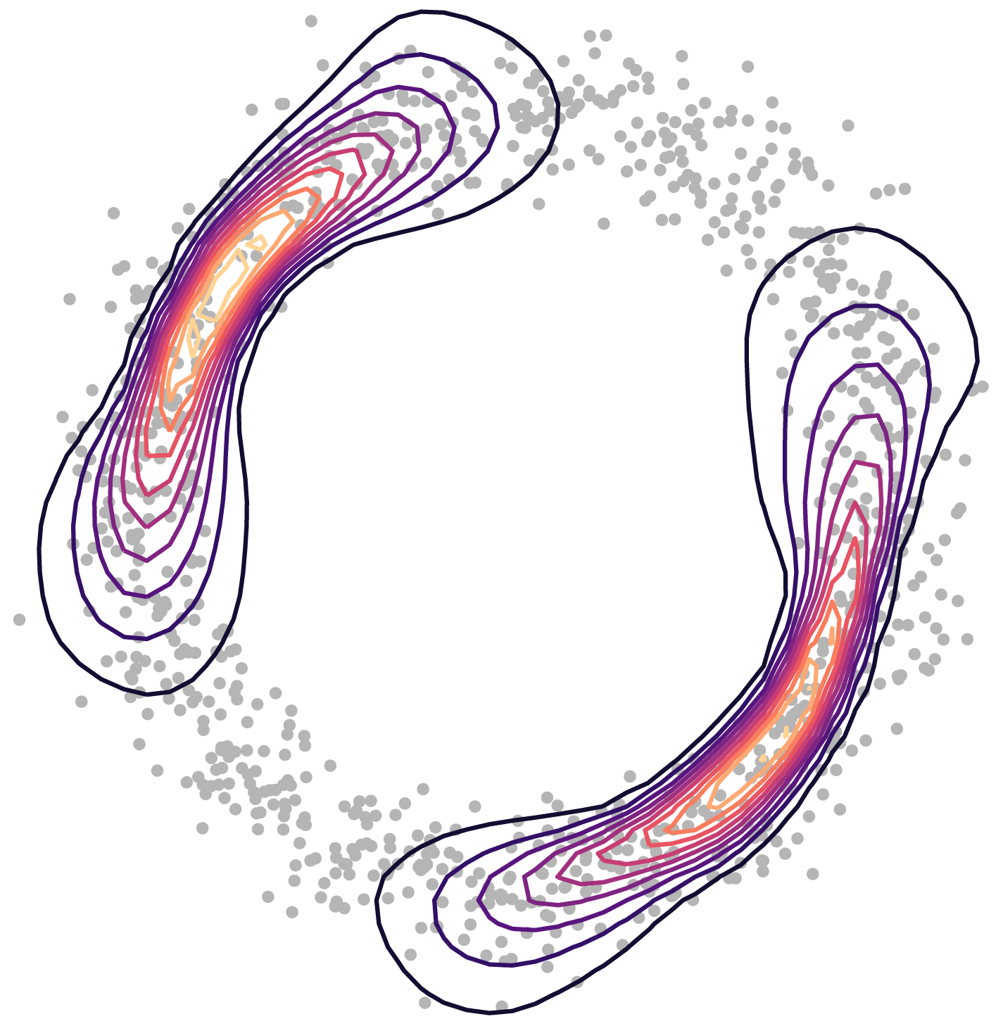
(a) land

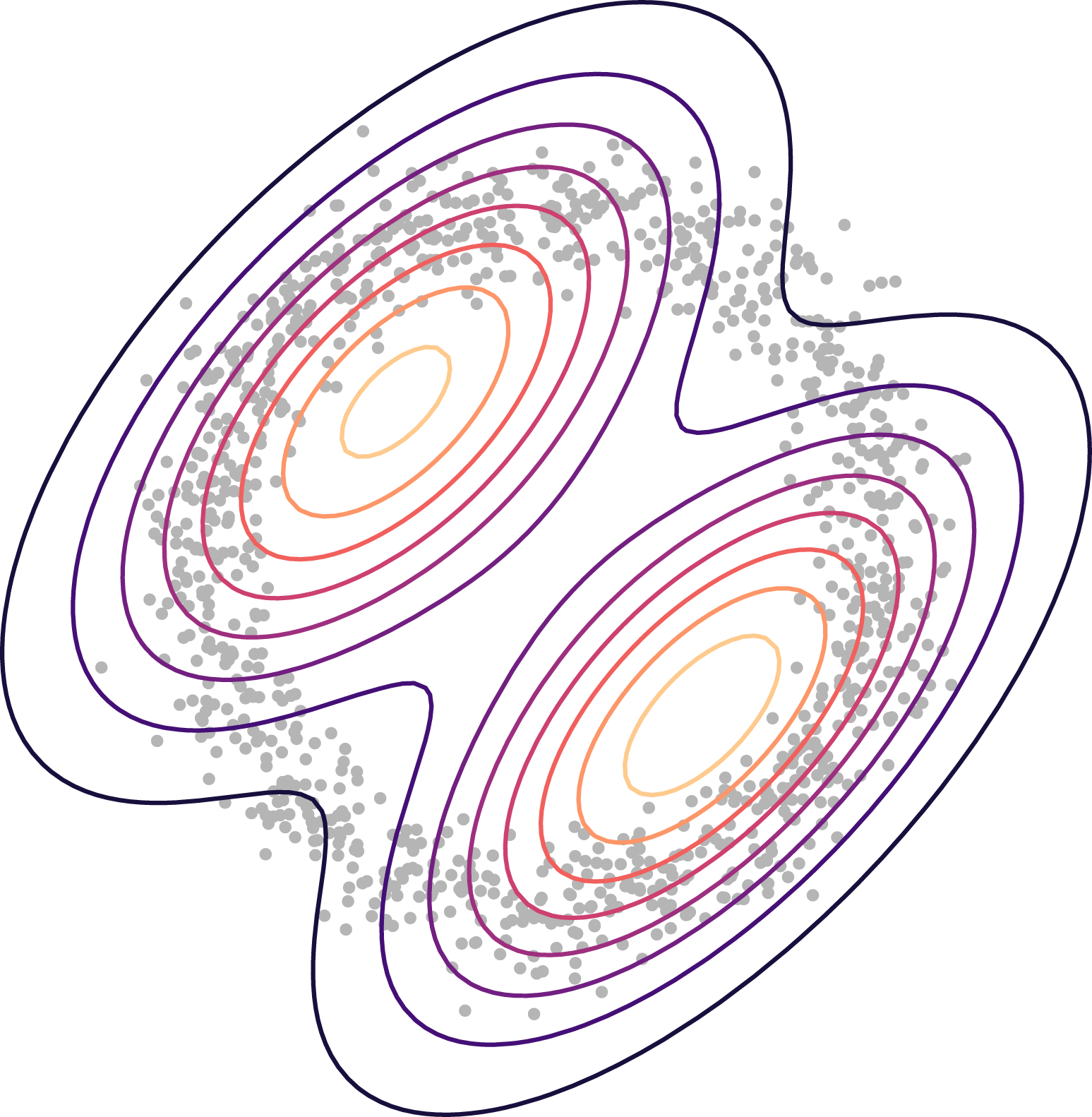
(b) gmm

Figure 8: Model comparison on circle toy data.

Higher-dimensional Toy Data

With increasing number of dimensions, new challenges for metric learning and geodesic solvers appear. With the simple kernel metric, almost all of the volume will be far from the data as the dimension increases, a phenomenon which we observe already in relatively low dimensions. Such metric behavior can lead to pathological integration problems, as the integrand may then become almost constant. In this experiment, we embed the circle toy data in higher dimensions by sampling random orthonormal matrices. After projecting the data, we add Gaussian noise $\epsilon_{i}\sim\mathcal{N}(0,0.01)$ and standardize. Here we show the result for $d=5$ and report results for $d=\{3,4\}$ in A.4.

5.2 Real-World Experiments

mnist

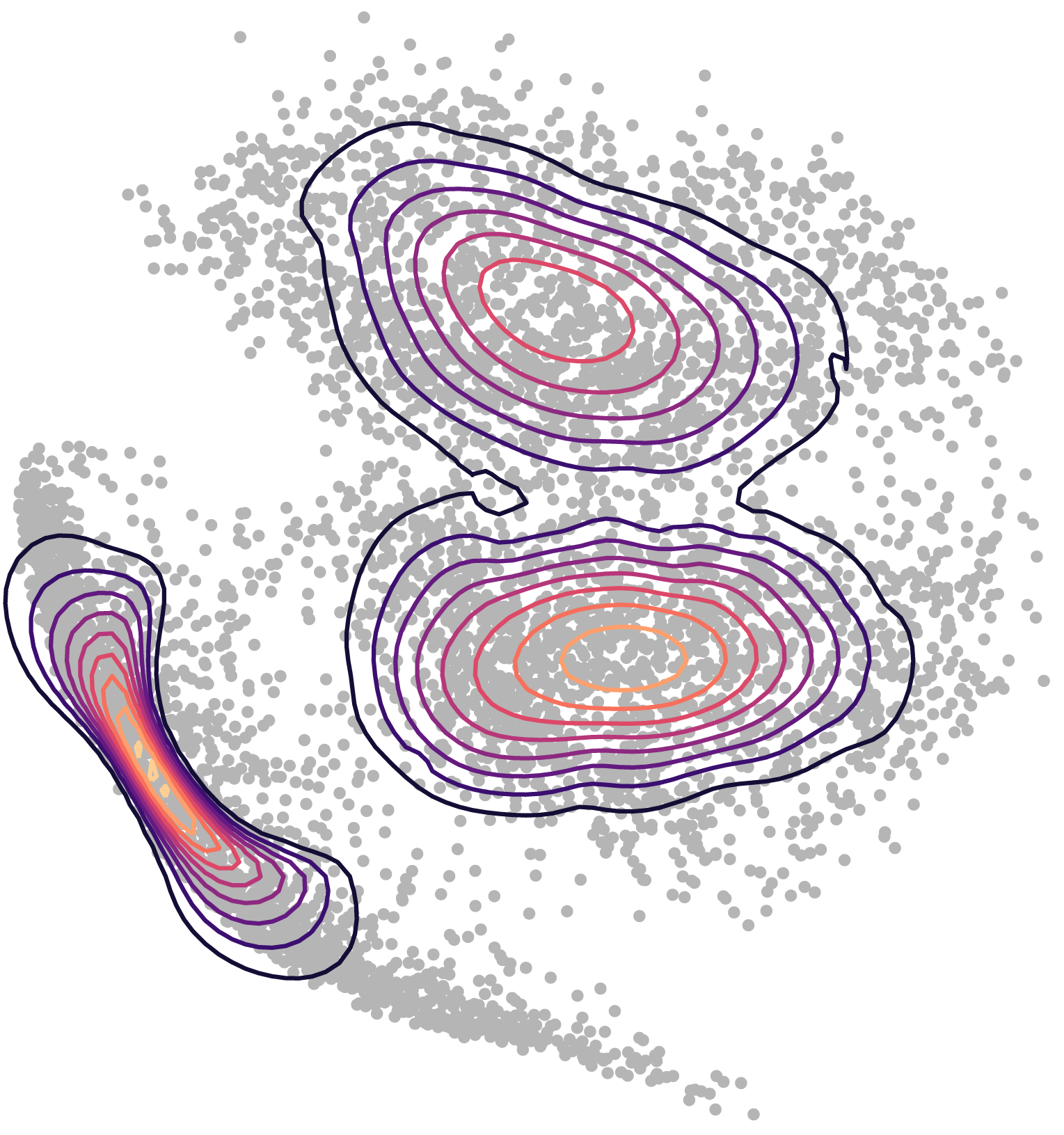
(a) land

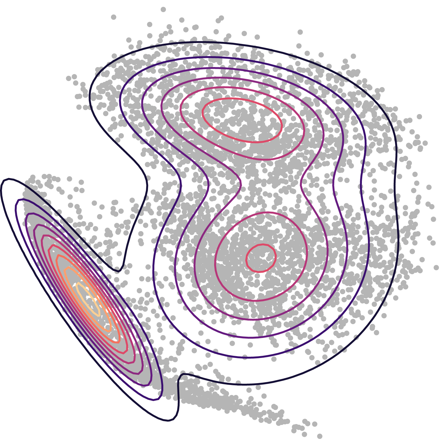
(b) gmm

Figure 9: Model comparison on three-digit mnist.

We trained a Variational Auto-Encoder on the first three digits of mnist using the aggregated posterior metric (Sec. 2.1) and found that the land is able to distinguish the three clusters more clearly than a Euclidean Gaussian mixture model, see Fig. 9. The land favors regions of higher density, where the vae has more training data. In this experiment, the gain in speed of bq is even more pronounced, since exponential maps are slow due to high curvature. mc with $1000$ samples achieves $2.78\%$ mean error on the whole land fit with a total runtime of $6$ hours and $56$ minutes, whereas dcv (18/2 exponential maps) achieves $2.84\%$ error within $21$ minutes; a speedup by a factor of $\approx 20$.

Molecular Dynamics

In molecular dynamics, biophysical systems are simulated on the atomic level. This approach is useful to understand the conformational changes of a protein, i.e., the structural changes it undergoes. A Riemannian model is appropriate in this setting, because not all atom coordinates represent physically realistic conformations. For instance, a protein clearly does not self-intersect. Adapting locally to the data by space distortion is thus critical for modeling. More specifically, the land model is relevant because clustering conformations and finding representative states are of scientific interest (see e.g., Papaleo et al., 2009; Wolf & Kirschner, 2013; Spellmon et al., 2015; Tribello & Gasparotto, 2019). The land can visualize the conformational landscape and generate realistic samples. Plausible interpolations (trajectories) between conformations may be conceived of as geodesics under the Riemannian metric.

We obtained multiple trajectories of the closed to open transition of the enzyme adenylate kinase (adk) (Seyler et al., 2015). Each observation consists of the Cartesian $(x,y,z)$ coordinates for each of the $3{,}341$ atoms, yielding a $10{,}023$ dimensional vector. As is common in the field, we used pca to extract the essential dynamics (Amadei et al., 1993), which clearly exhibit manifold structure (Fig. 1). The first two eigenvectors already explain $65\%$ of the total variance and suffice to capture the transition motion. We model the adk manifold with high curvature and large measure far from the data to account for the knowledge that realistic trajectories lie closely together. This makes for a challenging integration problem, since most mass is near the data boundary due to extreme metric values.

A single-component land yields a representative state for the transition between the closed and open conformation. Whereas the Euclidean mean falls outside the data manifold, the land mean is reasonably situated. Plotting the eigenvectors of the covariance matrix makes it clear that the land captures the intrinsic dimensions of the data manifold (Fig. 10) and that the mean interpolates between the closed and open state (Fig. 11).

Figure 10: Comparison of the Euclidean Gaussian vs. land mean and eigenvectors on adk data. Data is colored according to the radius of gyration, a measure indicating how “open” the protein is, providing a visual argument for the manifold hypothesis.

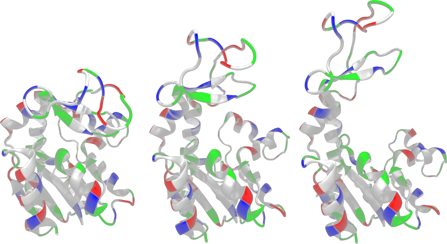
Figure 11: adk in closed, land mean and open state.

Our aim here is to demonstrate that molecular dynamics is an exciting application area for Riemannian statistics and sketch potential experiments, which are then for domain experts to design.

5.3 Interpretation

We find that bq consistently outperforms mc in terms of speed. Even on high-curvature manifolds with volume elements spanning multiple orders of magnitudes, such as mnist and adk, the gp succeeds to approximate the integrand well. Among the different bq candidates, we cannot discern a clear winner, since their performance depends on the specific problem geometry and exponential map runtimes. dcv performs especially well when geodesic computations are costly, such as for mnist. We note that geodesic solvers and metric learning are subject to new challenges in higher dimensions, which merit further research effort.

6 Conclusion and Discussion

Riemannian statistics is the appropriate framework to model real data with nonlinear geometry. Yet, its wide adoption is hampered by the prohibitive cost of numerical computations required to learn geometry from data and operate on manifolds. In this work, we have demonstrated on the example of numerical integration the great potential of probabilistic numerical methods (pnm) to reduce this computational burden. pnm adaptively select actions in a decision-theoretic manner and thus handle information with greater care than classic methods, e.g., Monte Carlo. Consequently, the deliberate choice of informative computations saves unnecessary operations on the manifold.

We have extended Bayesian quadrature to Riemannian manifolds, where it outperforms Monte Carlo over a large number of integration problems owing to its increased sample efficiency. Beyond known active learning schemes for bq, we have introduced a version of uncertainty sampling adapted to the manifold setting that allows to further reduce the number of expensive geodesic evaluations needed to estimate the integral.

Numerical integration is just one of multiple numerical tasks in the context of statistics on Riemannian manifolds where pnm suggest promising improvements. The key operations on data manifolds are geodesic computations, i.e., solutions of ordinary differential equations. Geodesics have been viewed through the pn lens, e.g., by Hennig & Hauberg (2014), but still offer a margin for increasing the performance of statistical models such as the considered land.

Once multiple pnm are established for Riemannian statistics, the future avenue directs towards having them operate in a concerted fashion. As data-driven Riemannian models rely on complex computation pipelines with multiple sources of epistemic and aleatory uncertainty, their robustness and efficiency can benefit from modeling and propagating uncertainty through the computations.

All in all, we believe the coalition of geometry- and uncertainty-aware methods to be a fruitful endeavor, as these approaches are united by their common intention to respect structure in data and computation that is otherwise often neglected.

Appendix A.1 Riemannian Geometry

A manifold $\mathcal{M}$ of dimension $D$ is a topological space which does not carry a global vector space structure. As opposed to the familiar $\mathbb{R}^{D}$, a manifold lacks the possibility of adding or scaling vectors globally. Instead, an atlas it used to cover the manifold in charts, which only locally give a Euclidean view of the manifold. If transition maps between overlapping charts are smooth, we call $\mathcal{M}$ a smooth manifold, which provides the means for doing calculus. Our analysis is heavily simplified by viewing $\mathbb{R}^{D}$ as a manifold and employing the identity map as a global chart map, which covers the whole $\mathbb{R}^{D}$, thereby endowing the manifold automatically with the smoothness property. We use global Euclidean coordinates, which implies that we can solve the geodesic equations directly in this global chart.

A.1.1 Geodesic Equations

The energy or action functional of a curve $\boldsymbol{\mathsf{\gamma}}$ with time derivative $\dot{\boldsymbol{\mathsf{\gamma}}}(t)$ is defined as

$$E(\boldsymbol{\mathsf{\gamma}})=\frac{1}{2}\int_{0}^{1}\underbrace{\langle\dot{\boldsymbol{\mathsf{\gamma}}}(t),\boldsymbol{\mathsf{M}}(\boldsymbol{\mathsf{\gamma}}(t))\dot{\boldsymbol{\mathsf{\gamma}}}(t)\rangle}_{\eqqcolon\mathscr{L}}\,\operatorname{d}\!t.$$ (12)

In physics, the argument of the integral is known as Lagrangian and we therefore abbreviate the inner product as $\mathscr{L}~{}\coloneqq~{}\langle\dot{\boldsymbol{\mathsf{\gamma}}}(t),\boldsymbol{\mathsf{M}}(\boldsymbol{\mathsf{\gamma}}(t))\dot{\boldsymbol{\mathsf{\gamma}}}(t)\rangle$. Geodesics are the stationary curves of this functional. We are interested in the minimizers, i.e., shortest paths. Minimizing curve energy instead of length avoids the issue of arbitrary reparameterization. Let $\gamma^{i}$ denote the $i$-th coordinate of the curve $\boldsymbol{\mathsf{\gamma}}$ at time $t$ and $M_{ik}$ the metric component at row $i$ and column $k$, if it is represented as a matrix. We leave sums over repeated indices implicit (Einstein summation convention). Applying the Euler-Lagrange equations to the functional $E$ results in a system of equations involving $\mathscr{L}$

$$\frac{\partial\mathscr{L}}{\partial\gamma^{k}}=\frac{\partial}{\partial t}\frac{\partial\mathscr{L}}{\partial\dot{\gamma}^{k}},\quad\text{for }k\in 1,\dots,D.$$ (13)

which is a system of $2^{nd}$ order differential equations. We first consider the left-hand side

$$\textup{I}\coloneqq\frac{\partial\mathscr{L}}{\partial\gamma^{k}}=\frac{1}{2}\frac{\partial M_{ij}}{\partial\gamma^{k}}\dot{\gamma}^{i}\dot{\gamma}^{j},$$ (14)

which holds due to independence of the coordinates. The right-hand side is

$$\textup{II}\coloneqq\frac{\partial}{\partial t}\left[M_{ik}\dot{\gamma}^{i}\right]=\frac{\partial M_{ik}}{\partial\gamma^{j}}\dot{\gamma}^{i}\dot{\gamma}^{j}+M_{ik}\ddot{\gamma}^{i}.$$ (15)

We expand this using a small index rearrangement trick

$$\textup{II}=\frac{1}{2}\frac{\partial M_{ik}}{\partial\gamma^{j}}\dot{\gamma}^{i}\dot{\gamma}^{j}+\frac{1}{2}\frac{\partial M_{jk}}{\partial\gamma^{i}}\dot{\gamma}^{i}\dot{\gamma}^{j}+M_{ik}\ddot{\gamma}^{i}.$$ (16)

This allows us to write $\textup{I}=\textup{II}\Leftrightarrow\textup{II}-\textup{I}=0$ as

$$M_{ik}\ddot{\gamma}^{i}+\frac{1}{2}\left(\frac{\partial M_{ik}}{\partial\gamma^{j}}+\frac{\partial M_{jk}}{\partial\gamma^{i}}-\frac{\partial M_{ij}}{\partial\gamma^{k}}\right)\dot{\gamma}^{j}=0.$$ (17)

the next step is to left multiply with the inverse metric tensor and plug in the Christoffel symbols defined as follows

$$\Gamma_{ij}^{k}=\frac{1}{2}M^{-1}_{kh}\left(\frac{\partial M_{ih}}{\partial\gamma^{j}}+\frac{\partial M_{jh}}{\partial\gamma^{i}}-\frac{\partial M_{ij}}{\partial\gamma^{h}}\right),$$ (18)

so we finally obtain the geodesic equations in the canonical form

$$\ddot{\gamma}^{k}+\Gamma_{ij}^{k}\dot{\gamma}^{j}\dot{\gamma}^{j}=0,\quad\text{for }k\in 1,\dots,D.$$ (19)

We assume our manifold to be geodesically complete (Pennec, 2006), which means that geodesics can be infinitely extended, i.e., their domain is $\mathbb{R}$. As a consequence, the exponential map is then defined on the whole tangent space. In theory, the exponential map $\operatorname{Exp}_{\boldsymbol{\mathsf{\mu}}}(\cdot)$ is a diffeomorphism only in some open neighborhood around $\boldsymbol{\mathsf{\mu}}$ and thus it only admits a smooth inverse, i.e., $\operatorname{Log}_{\boldsymbol{\mathsf{\mu}}}(\cdot)$, in said neighborhood. However, we assume this to be true on the whole manifold in practice to keep the analysis tractable. For long geodesics on high-curvature data manifolds, often $\operatorname{Log}_{\boldsymbol{\mathsf{\mu}}}(\operatorname{Exp}_{\boldsymbol{\mathsf{\mu}}}(\boldsymbol{\mathsf{v}}))\neq\boldsymbol{\mathsf{v}}$. This is rather unproblematic since if $\|\operatorname{Log}_{\boldsymbol{\mathsf{\mu}}_{l}}(\boldsymbol{\mathsf{x}}_{n})\|$ is high, the responsibility $r_{nl}$ will be low (see A.2), so this logarithmic map will play a minimal role in the Mahalanobis distance of the land density. Thus, the optimization process on its own favors mean and covariances such that the density is concentrated in sufficiently small neighborhoods where the exponential map approximately admits an inverse.

A.1.2 Covariance and Precision Matrices

We here elaborate on Footnote 1 of the paper. The Riemannian normal distribution (Pennec, 2006) is defined using the precision matrix $\boldsymbol{\mathsf{\Gamma}}$. This matrix lives on the tangent space $\mathcal{T}_{\boldsymbol{\mathsf{\mu}}}\mathcal{M}$, i.e., it may be represented as a matrix in $\mathbb{R}^{D\times D}$, where $D$ is the dimension of the tangent space, which is equal to the topological dimension of the manifold. In our applied setting, $D$ matches the dimension of the data space, as we view the whole $\mathbb{R}^{D}$ as the manifold. We can use the tangent space “covariance” matrix $\boldsymbol{\mathsf{\Sigma}}=\boldsymbol{\mathsf{\Gamma}}^{-1}$ for our reasoning and the optimization process. However, to obtain the true covariance on the manifold $\mathcal{M}$, a subtle correction is necessary (Pennec, 2006)

$$\boldsymbol{\mathsf{\Sigma}}_{\mathcal{M}}=\mathbb{E}\left[\operatorname{Log}_{\boldsymbol{\mathsf{\mu}}}(\boldsymbol{\mathsf{x}})\operatorname{Log}_{\boldsymbol{\mathsf{\mu}}}(\boldsymbol{\mathsf{x}})^{\intercal}\right]=\frac{1}{\mathcal{C}}\int_{\mathcal{M}}\operatorname{Log}_{\boldsymbol{\mathsf{\mu}}}(\boldsymbol{\mathsf{x}})\operatorname{Log}_{\boldsymbol{\mathsf{\mu}}}(\boldsymbol{\mathsf{x}})^{\intercal}\exp\left(-\frac{1}{2}\left\langle\operatorname{Log}_{\boldsymbol{\mathsf{\mu}}}(\boldsymbol{\mathsf{x}}),\boldsymbol{\mathsf{\Gamma}}\operatorname{Log}_{\boldsymbol{\mathsf{\mu}}}(\boldsymbol{\mathsf{x}})\right\rangle\right)\,\operatorname{d}\!\mathcal{M}(\boldsymbol{\mathsf{x}}),$$ (20)

with respect to the density on the manifold. For conceptual ease, we focus on the tangent space view in the paper. To plot the eigenvectors of the adk land covariance (Fig. 10), we used the exponential map on the tangent space covariance matrix, i.e., we evaluate and plot $\operatorname{Exp}_{\boldsymbol{\mathsf{\mu}}}(\boldsymbol{\mathsf{v}}_{1:2})$, where $\boldsymbol{\mathsf{v}}_{1:2}$ are the eigenvectors of $\boldsymbol{\mathsf{\Sigma}}$.

A.1.3 Geodesic Solvers

To solve the geodesic equations, we combine two solvers, which have different strengths and weaknesses. By chaining them together, we obtain a more robust computational pipeline.

First, we make use of the fast and robust fixed-point solver (fp) introduced by Arvanitidis et al. (2019a). This solver pursues a gp-based approach that avoids the often ill-behaved Jacobians of the geodesic ode system. However, the resulting logarithmic maps are subject to significant approximation error, depending on the curvature of the manifold. The parameters of this solver are as follows:

Parameter	Value	Description
$\mathtt{iter_{max}}$	$1000$	maximum number of iterations
$\mathtt{N}$	$10$	number of mesh nodes.
$\mathtt{tol}$	$0.1$	tolerance used to evaluate solution correctness.
$\mathtt{\sigma}$	$10^{-4}$	noise of the gp.

For mnist, we set $\mathtt{iter_{max}}=500$, and $\mathtt{tol}=0.2$, since this high-curvature manifold easily leads to failing geodesics.

The second solver we employ is a precise, albeit less robust one. This is the bvp solver available in the module scipy.integrate.solve_bvp. On high-curvature manifolds, this solver often fails (especially for long curves) and takes a significant amount of time to run. When it succeeds, however, the logarithmic maps are reliable. For this solver, we set the maximum number of mesh nodes to $100$ and the tolerance to $0.1$. We empirically found that choosing a high maximum number of mesh nodes (e.g., $500$) can lead to high runtimes for failing geodesic computations.

To obtain fast and robust geodesics, these solvers may be chained together, i.e., we initialize the bvp solver with the fp solution, which is often worth the extra effort for speedup and improved robustness. For initialization, we use $20$ mesh nodes, evenly spaced on the fp solution. If the fp solver already failed, it is very unlikely for the bvp solver to succeed, so we abort the computation.

Furthermore, we exploit previously computed bvp solutions: assume we want to compute $\operatorname{Log}_{\boldsymbol{\mathsf{\mu}}_{t}}(\boldsymbol{\mathsf{x}})$. We search for past results $\operatorname{Log}_{\boldsymbol{\mathsf{\mu}}_{t}^{*}}(\boldsymbol{\mathsf{x}})$, with $t^{*}<t$, $t^{*}=\operatorname*{arg\>min}\|\boldsymbol{\mathsf{\mu}}_{t}-\boldsymbol{\mathsf{\mu}}_{t*}\|$ and $\|\boldsymbol{\mathsf{\mu}}_{t}-\boldsymbol{\mathsf{\mu}}_{t*}\|<\epsilon_{d}$, where we choose $\epsilon_{d}=0.5$. Since we compute logarithmic maps for data points $\boldsymbol{\mathsf{x}}_{1:N}$, which do not change during land optimization, we can use them as hash keys in a dictionary, where we store the solutions. Looking up the solution is then linear in the number of previous land iterations. If such a solution is found, the fp is skipped and the solution is used to directly initialize the bvp solver.

For the exponential maps, we use scipy.integrate.solve_ivp with a tolerance of $10^{-3}$.

Appendix A.2 The land Objective and Gradients

Given a dataset $\boldsymbol{\mathsf{x}}_{1:N}$ assumed to be i.i.d., the negative log-likelihood of the Locally Adaptive Normal Distribution (LAND) mixture can be stated as (Arvanitidis et al., 2016)

$$\mathcal{L}\left(\{\boldsymbol{\mathsf{\mu}}_{k},\boldsymbol{\mathsf{\Sigma}}_{k}\}_{1:K}\right)=\sum_{k=1}^{K}\sum_{n=1}^{N}r_{nk}\left[\frac{1}{2}\langle\operatorname{Log}_{\boldsymbol{\mathsf{\mu}}_{k}}(\boldsymbol{\mathsf{x}}_{n}),\boldsymbol{\mathsf{\Sigma}}_{k}^{-1}\operatorname{Log}_{\boldsymbol{\mathsf{\mu_{k}}}}(\boldsymbol{\mathsf{x}}_{n})\rangle+\log\left(\mathcal{C}(\boldsymbol{\mathsf{\mu}}_{k},\boldsymbol{\mathsf{\Sigma}}_{k})\right)-\log(\pi_{k})\right]$$ (21)

where $\pi_{k}$ is the weight of the $k^{\text{th}}$ component, $\sum_{k=1}^{K}\pi_{k}=1$ and $r_{nk}=\frac{\pi_{k}p(x_{n}\mid\boldsymbol{\mathsf{\mu}}_{k},\boldsymbol{\mathsf{\Sigma}}_{k})}{\sum_{l=1}^{K}\pi_{l}p(x_{n}\mid\boldsymbol{\mathsf{\mu}}_{l},\boldsymbol{\mathsf{\Sigma}}_{l})}$ is the responsibility of the $k^{\text{th}}$ component for the $n^{\text{th}}$ datum. The maximum likelihood solution can be obtained by non-convex optimization, alternating between gradient descent updates of $\boldsymbol{\mathsf{\mu}}$ and $\boldsymbol{\mathsf{\Sigma}}$ and cycling through the components $k$, as described in Alg. 1.

Algorithm 1 land mixture main loop

  Input: data $\boldsymbol{\mathsf{x}}_{1:N}$, manifold $\mathcal{M}$ with $\operatorname{Exp}$ and $\operatorname{Log}$ operators, max. number of iterations $t_{max}$, initial stepsize $\alpha_{\boldsymbol{\mathsf{\mu}}}^{1}\in\mathbb{R}$, gradient tolerance $\epsilon_{\nabla_{\boldsymbol{\mathsf{\mu}}}}$, likelihood tolerance $\epsilon_{\mathcal{L}}$

  Output: estimates $\left(\boldsymbol{\mathsf{\mu}}_{k},\boldsymbol{\mathsf{\Sigma}}_{k},\mathcal{C}_{k},\pi_{k}\right)_{1:K}$

  Initialize land parameters$\left(\boldsymbol{\mathsf{\mu}}_{k}^{1},\boldsymbol{\mathsf{\Sigma}}_{k}^{1},\mathcal{C}_{k}^{1},\pi_{k}^{1}\right)_{1:K}$, $t\leftarrow 1$.

  repeat

     Expectation step: $r_{nk}=\frac{\pi_{k}p(x_{n}\mid\boldsymbol{\mathsf{\mu}}_{k},\boldsymbol{\mathsf{\Sigma}}_{k})}{\sum_{l=1}^{K}\pi_{l}p(x_{n}\mid\boldsymbol{\mathsf{\mu}}_{l},\boldsymbol{\mathsf{\Sigma}}_{l})}$

     Maximization step:

     for $k=1$ to $K$ do

        Compute $\mathcal{C}_{k}^{t}(\boldsymbol{\mathsf{\mu}}_{k}^{t},\boldsymbol{\mathsf{\Sigma}}_{k}^{t})$

        Compute $d_{\boldsymbol{\mathsf{\mu}}_{k}}\mathcal{L}(\boldsymbol{\mathsf{\mu}}_{k}^{t},\boldsymbol{\mathsf{\Sigma}}_{k}^{t})$ using Eq. (22)

        if $||d_{\boldsymbol{\mathsf{\mu}}_{k}}\mathcal{L}||<\epsilon_{\nabla_{\boldsymbol{\mathsf{\mu}}}}$ then

           Continue

        end if

        $\boldsymbol{\mathsf{\mu}}_{k}^{t+1}\leftarrow\operatorname{Exp}_{\boldsymbol{\mathsf{\mu}}_{k}^{t}}(\alpha_{\boldsymbol{\mathsf{\mu}}}^{t}d_{\boldsymbol{\mathsf{\mu}}_{k}}\mathcal{L})$

        Compute $\operatorname{Log}_{\boldsymbol{\mathsf{\mu}}_{k}^{t+1}}(\boldsymbol{\mathsf{x}}_{1:N})$

        Compute $\mathcal{C}_{k}^{t+1}(\boldsymbol{\mathsf{\mu}}_{k}^{t+1},\boldsymbol{\mathsf{\Sigma}}_{k}^{t})$

        $\boldsymbol{\mathsf{\Sigma}}_{k}^{t+1}\leftarrow\text{update}_{\boldsymbol{\mathsf{\Sigma}}_{k}^{t}}$ using Alg. 2

        $\pi_{k}^{t}=\frac{1}{N}\sum_{n=1}^{N}r_{nk}$

     end for

     if $\mathcal{L}^{t+1}<\mathcal{L}^{t}$ then

        $\alpha_{\boldsymbol{\mathsf{\mu}}}^{t+1}\leftarrow 1.1\cdot\alpha_{\boldsymbol{\mathsf{\mu}}}^{t}$ {optimism}

     else

        $\alpha_{\boldsymbol{\mathsf{\mu}}}^{t+1}\leftarrow 0.75\cdot\alpha_{\boldsymbol{\mathsf{\mu}}}^{t}$ {pessimism}

     end if

     $t\leftarrow t+1$

  until $||\mathcal{L}^{t+1}-\mathcal{L}^{t}||\leq\epsilon_{\mathcal{L}}$ or $t=t_{max}$

Algorithm 2 land $\text{update}_{\boldsymbol{\mathsf{\Sigma}}_{k}}$ on the symmetric positive definite manifold $\mathcal{S}_{+}$

  Input: Covariance $\boldsymbol{\mathsf{\Sigma}}_{k}^{t}$, mean $\boldsymbol{\mathsf{\mu}}_{k}$, max. linesearch iterations $t_{max,\boldsymbol{\mathsf{\Sigma}}}$, last stepsize $\alpha_{k}$, initial stepsize $\alpha_{1}=1.0$, sufficient decrease factor $c_{0}=0.5$, contraction factor $c_{1}=0.5$

  Output: $\boldsymbol{\mathsf{\Sigma}}_{k}^{t+1}$, $\alpha_{k}$ (for reuse)

  

  {define the exp. map on the $\mathcal{S}_{+}$ manifold, where $\boldsymbol{\mathsf{X}}$ is an SPD matrix and $\boldsymbol{\mathsf{\Xi}}$ is a tangent vector, i.e., a symmetric matrix}

  Function $\operatorname{Exp}_{\boldsymbol{\mathsf{X}}}^{+}(\boldsymbol{\mathsf{\Xi}})$:

   return $\boldsymbol{\mathsf{X}}^{\frac{1}{2}}\exp\left(\boldsymbol{\mathsf{X}}^{-\frac{1}{2}}\boldsymbol{\mathsf{\Xi}}\boldsymbol{\mathsf{X}}^{-\frac{1}{2}}\right)\boldsymbol{\mathsf{X}}^{\frac{1}{2}}$,  where $\exp$ denotes the matrix exponential.

  EndFunction

  {define the norm of a vector $\boldsymbol{\mathsf{\Xi}}$ in the tangent space of $\boldsymbol{\mathsf{X}}\in\mathcal{S}_{+}$}

  Function $\left(\|\cdot\|_{\boldsymbol{\mathsf{X}}}^{+}\right)(\boldsymbol{\mathsf{\Xi}})$:

   $\boldsymbol{\mathsf{X}}\leftarrow\boldsymbol{\mathsf{L}}\boldsymbol{\mathsf{L}}^{\intercal}$ {cholesky decomposition}

   return $\|\boldsymbol{\mathsf{L}}^{-1}\boldsymbol{\mathsf{\Xi}}\boldsymbol{\mathsf{L}}^{-\intercal}\|_{2}$

  EndFunction

  

  for $i=1$ to $2$ {outer gradient descent loop} do

     Compute (or retrieve from cache) $\mathcal{L}(\boldsymbol{\mathsf{\Sigma}}_{k}^{t})$

     Compute (or retrieve from cache) Euclidean gradient $\nabla_{\boldsymbol{\mathsf{\Sigma}}_{k}^{t}}\mathcal{L}(\Sigma_{k}^{t})$ using Eq. (25)

     Obtain manifold gradient: $g\coloneqq\nabla_{\boldsymbol{\mathsf{\Sigma}}_{k}^{t};\mathcal{S}_{+}}=\frac{1}{2}\boldsymbol{\mathsf{\Sigma}}_{k}^{t}\left(\nabla_{\boldsymbol{\mathsf{\Sigma}}_{k}^{t}}+\nabla_{\boldsymbol{\mathsf{\Sigma}}_{k}^{t}}^{\intercal}\right)\boldsymbol{\mathsf{\Sigma}}_{k}^{t}$

     if $\alpha_{k}$ is None or $\alpha_{k}=0$ then

        $\alpha_{k}\leftarrow\frac{\alpha_{0}}{\|g\|}$

     end if

     $\boldsymbol{\mathsf{\Sigma}}_{k}^{t+1}\leftarrow\operatorname{Exp}_{\boldsymbol{\mathsf{\Sigma}}_{k}^{t}}^{+}\left(-\alpha_{k}\cdot g\right)$

     Compute $\mathcal{C}_{k}(\boldsymbol{\mathsf{\mu}}_{k},\boldsymbol{\mathsf{\Sigma}}_{k}^{t+1})$

     Evaluate land objective $\mathcal{L}(\boldsymbol{\mathsf{\Sigma}}_{k}^{t+1})$

     {Linesearch subroutine}

     $j\leftarrow 1$

     while $\mathcal{L}(\boldsymbol{\mathsf{\Sigma}}_{k}^{t+1})>\mathcal{L}(\boldsymbol{\mathsf{\Sigma}}_{k}^{t})-c_{0}\cdot\alpha_{k}\cdot\|g\|^{2}$ and $j\leq t_{max,\boldsymbol{\mathsf{\Sigma}}}$ do

        {while no sufficient decrease, contract}

        $\alpha_{k}\leftarrow\alpha_{k}\cdot c_{1}$

        $\boldsymbol{\mathsf{\Sigma}}_{k}^{t+1}\leftarrow\operatorname{Exp}_{\boldsymbol{\mathsf{\Sigma}}_{k}^{t}}^{+}\left(-\alpha_{k}\cdot g\right)$

        Compute $\mathcal{C}_{k}(\boldsymbol{\mathsf{\mu}}_{k},\boldsymbol{\mathsf{\Sigma}}_{k}^{t+1})$

        Evaluate land objective $\mathcal{L}(\boldsymbol{\mathsf{\Sigma}}_{k}^{t+1})$

        $j\leftarrow j+1$

     end while

     if $\mathcal{L}(\boldsymbol{\mathsf{\Sigma}}_{k}^{t+1})>\mathcal{L}(\boldsymbol{\mathsf{\Sigma}}_{k}^{t})$ then

        $\alpha_{k}\leftarrow 0$

     end if

     if $j\neq 2$ then

        $\alpha_{k}=1.3\cdot\alpha_{k}$ {optimism}

     end if

     $t\leftarrow t+1$

  end for

For $\boldsymbol{\mathsf{\mu}}$, we use the steepest descent direction as in Arvanitidis et al. (2016)

$$d_{\boldsymbol{\mathsf{\mu}}_{k}}\mathcal{L}=\sum_{n=1}^{N}r_{nk}\operatorname{Log}_{\boldsymbol{\mathsf{\mu}}_{k}}(\boldsymbol{\mathsf{x}}_{n})-\frac{\mathcal{Z}_{k}\cdot R_{k}}{\mathcal{C}_{k}(\boldsymbol{\mathsf{\mu}}_{k},\boldsymbol{\mathsf{\Sigma}}_{k})}\int_{\mathcal{T}_{\boldsymbol{\mathsf{\mu}}_{k}}\mathcal{M}}\boldsymbol{\mathsf{v}}g_{\boldsymbol{\mathsf{\mu}}_{k}}(\boldsymbol{\mathsf{v}})\mathcal{N}(\boldsymbol{\mathsf{v}};\boldsymbol{\mathsf{0}},\boldsymbol{\mathsf{\Sigma}}_{k})\,\operatorname{d}\!\boldsymbol{\mathsf{v}},$$ (22)

where the vector-valued integral stems from bq and $R_{k}=\sum_{n=1}^{N}r_{nk}$, $\mathcal{Z}_{k}=\sqrt{(2\pi)^{d}|\boldsymbol{\mathsf{\Sigma}}_{k}|}$.

Arvanitidis et al. (2016) decomposed the precision $\boldsymbol{\mathsf{\Sigma}}_{k}^{-1}=\boldsymbol{\mathsf{A}}^{\intercal}\boldsymbol{\mathsf{A}}$ for unconstrained optimization using gradient descent. We opt for a more principled approach by exploiting geometric structure of the symmetric positive definite (SPD) manifold, to which the covariance is confined. More specifically, we use the bi-invariant metric (Bhatia, 2009). Under this metric, geodesics from $\boldsymbol{\mathsf{A}}$ to $\boldsymbol{\mathsf{B}}$ may be parameterized as $\gamma(t)~{}=\boldsymbol{\mathsf{A}}^{\frac{1}{2}}\left(\boldsymbol{\mathsf{A}}^{-\frac{1}{2}}\boldsymbol{\mathsf{B}}^{\frac{1}{2}}\boldsymbol{\mathsf{A}}^{-\frac{1}{2}}\right)^{t}\boldsymbol{\mathsf{A}}^{\frac{1}{2}},\quad 0\leq t<1$, and the distance from $\boldsymbol{\mathsf{A}}$ to $\boldsymbol{\mathsf{B}}$ is $d(\boldsymbol{\mathsf{A}},\boldsymbol{\mathsf{B}})~{}=\left\|\log{\boldsymbol{\mathsf{A}}^{-\frac{1}{2}}\boldsymbol{\mathsf{B}}^{\frac{1}{2}}\boldsymbol{\mathsf{A}}^{-\frac{1}{2}}}\right\|_{2}$. The name stems from the fact that this distance is invariant under multiplication with any invertible square matrix $\boldsymbol{\mathsf{\Xi}}$, i.e., $d(\boldsymbol{\mathsf{A}},\boldsymbol{\mathsf{B}})~{}=d(\boldsymbol{\mathsf{\Xi}}\cdot\boldsymbol{\mathsf{A}},\boldsymbol{\mathsf{\Xi}}\cdot\boldsymbol{\mathsf{B}})$. For manifold gradient descent, we calculate the Euclidean gradient and then project it onto the manifold. We begin with the first term

$$\nabla_{\boldsymbol{\mathsf{\Sigma}}_{k}}\left(\sum_{n=1}^{N}r_{nk}\left[\frac{1}{2}\langle\operatorname{Log}_{\boldsymbol{\mathsf{\mu}}_{k}}(\boldsymbol{\mathsf{x}}_{n}),\boldsymbol{\mathsf{\Sigma}}_{k}^{-1}\operatorname{Log}_{\boldsymbol{\mathsf{\mu_{k}}}}(\boldsymbol{\mathsf{x}}_{n})\rangle\right]\right)=-\frac{1}{2}\sum_{n=1}^{N}r_{nk}\boldsymbol{\mathsf{\Sigma}}_{k}^{-\intercal}\operatorname{Log}_{\boldsymbol{\mathsf{\mu_{k}}}}(\boldsymbol{\mathsf{x}}_{n})\operatorname{Log}_{\boldsymbol{\mathsf{\mu_{k}}}}(\boldsymbol{\mathsf{x}}_{n})^{\intercal}\boldsymbol{\mathsf{\Sigma}}_{k}^{-\intercal}.$$ (23)

For the gradient of the normalization constant we get

$$\nabla_{\boldsymbol{\mathsf{\Sigma}}_{k}}\log(\mathcal{C}(\boldsymbol{\mathsf{\mu}}_{k},\boldsymbol{\mathsf{\Sigma}}_{k})) =\frac{1}{\mathcal{C}(\boldsymbol{\mathsf{\mu}}_{k},\boldsymbol{\mathsf{\Sigma}}_{k})}\int_{\mathcal{M}}\nabla_{\boldsymbol{\mathsf{\Sigma}}_{k}}\exp\left(\frac{1}{2}\langle\operatorname{Log}_{\boldsymbol{\mathsf{\mu}}_{k}}(\boldsymbol{\mathsf{x}}),\boldsymbol{\mathsf{\Sigma}}^{-1}\operatorname{Log}_{\boldsymbol{\mathsf{\mu}}_{k}}(\boldsymbol{\mathsf{x}})\rangle\right)\,\operatorname{d}\!\mathcal{M}_{\boldsymbol{\mathsf{x}}}$$ (24)

$$=\frac{1}{2\cdot\mathcal{C}(\boldsymbol{\mathsf{\mu}}_{k},\boldsymbol{\mathsf{\Sigma}}_{k})}\int_{\mathcal{M}}\boldsymbol{\mathsf{\Sigma}}_{k}^{-\intercal}\operatorname{Log}_{\boldsymbol{\mathsf{\mu}}_{k}}(\boldsymbol{\mathsf{x}})\operatorname{Log}_{\boldsymbol{\mathsf{\mu}}_{k}}(\boldsymbol{\mathsf{x}})^{\intercal}\boldsymbol{\mathsf{\Sigma}}_{k}^{-\intercal}\exp\left(-\frac{1}{2}\langle\operatorname{Log}_{\boldsymbol{\mathsf{\mu}}_{k}}(\boldsymbol{\mathsf{x}}),\boldsymbol{\mathsf{\Sigma}}^{-1}\operatorname{Log}_{\boldsymbol{\mathsf{\mu}}_{k}}(\boldsymbol{\mathsf{x}})\rangle\right)\,\operatorname{d}\!\mathcal{M}_{\boldsymbol{\mathsf{x}}}$$

$$=\frac{1}{2\cdot\mathcal{C}(\boldsymbol{\mathsf{\mu}}_{k},\boldsymbol{\mathsf{\Sigma}}_{k})}\int_{\mathcal{T}_{\boldsymbol{\mathsf{\mu}}_{k}}\mathcal{M}}\boldsymbol{\mathsf{\Sigma}}_{k}^{-\intercal}\boldsymbol{\mathsf{v}}\boldsymbol{\mathsf{v}}^{\intercal}g_{\boldsymbol{\mathsf{\mu}}_{k}}(\boldsymbol{\mathsf{v}})\boldsymbol{\mathsf{\Sigma}}_{k}^{-\intercal}\exp\left(-\frac{1}{2}\langle\boldsymbol{\mathsf{v}},\boldsymbol{\mathsf{\Sigma}}^{-1}\boldsymbol{\mathsf{v}}\rangle\right)\,\operatorname{d}\!\boldsymbol{\mathsf{v}}.$$

Taking this together, we obtain the gradient

$$\nabla_{\boldsymbol{\mathsf{\Sigma}}_{k}}\mathcal{L}= -\frac{1}{2}\sum_{n=1}^{N}r_{nk}\boldsymbol{\mathsf{\Sigma}}_{k}^{-\intercal}\operatorname{Log}_{\boldsymbol{\mathsf{\mu_{k}}}}(\boldsymbol{\mathsf{x}}_{n})\operatorname{Log}_{\boldsymbol{\mathsf{\mu_{k}}}}(\boldsymbol{\mathsf{x}}_{n})^{\intercal}\boldsymbol{\mathsf{\Sigma}}_{k}^{-\intercal}$$ (25)

$$+\frac{R_{k}}{2\cdot\mathcal{C}(\boldsymbol{\mathsf{\mu}}_{k},\boldsymbol{\mathsf{\Sigma}}_{k})}\int_{\mathcal{T}_{\boldsymbol{\mathsf{\mu}}_{k}}\mathcal{M}}\boldsymbol{\mathsf{\Sigma}}_{k}^{-\intercal}\boldsymbol{\mathsf{v}}\boldsymbol{\mathsf{v}}^{\intercal}g_{\boldsymbol{\mathsf{\mu}}_{k}}(\boldsymbol{\mathsf{v}})\boldsymbol{\mathsf{\Sigma}}_{k}^{-\intercal}\exp\left(-\frac{1}{2}\langle\boldsymbol{\mathsf{v}},\boldsymbol{\mathsf{\Sigma}}^{-1}\boldsymbol{\mathsf{v}}\rangle\right)\,\operatorname{d}\!\boldsymbol{\mathsf{v}},$$

where the matrix-valued integral again stems from bq. To project the Euclidean gradient $\nabla_{\boldsymbol{\mathsf{\Sigma}}_{k}}$ onto the tangent space of a SPD matrix $\boldsymbol{\mathsf{\Sigma}}_{k}$, we simply calculate $\frac{1}{2}\boldsymbol{\mathsf{\Sigma}}_{k}\left(\nabla_{\boldsymbol{\mathsf{\Sigma}}_{k}}+\nabla_{\boldsymbol{\mathsf{\Sigma}}_{k}}^{\intercal}\right)\boldsymbol{\mathsf{\Sigma}}_{k}$. We optimize with gradient descent and a deterministic manifold linesearch as a subroutine, which adaptively chooses its step lengths. This procedure as well as the SPD manifold are conveniently available in the Pymanopt (Townsend et al., 2016) library.

In sum, the optimization process is as follows: we cycle through the components $K$. After taking a single steepest-direction step for $\boldsymbol{\mathsf{\mu}}_{k}$, we perform two gradient descent steps for $\boldsymbol{\mathsf{\Sigma}}_{k}$, each of which may use up to $4$ steps in the linesearch subroutine to satisfy a sufficient decrease criterion. We provide pseudocode for the covariance update in Alg. 2. The optimizer has the following hyperparameters:

Parameter	Value	Description
$t_{max}$	-	update each component $\mathtt{t_{max}}$ times.
$\alpha_{\boldsymbol{\mathsf{\mu}}}^{1}$	-	initial stepsize for mean updates.
$\epsilon_{\nabla_{\boldsymbol{\mathsf{\mu}}}}$	-	tolerance for mean gradients
$\epsilon_{\mathcal{L}}$	$2$	likelihood tolerance
$t_{max,\boldsymbol{\mathsf{\Sigma}}}$	$4$	max. $\boldsymbol{\mathsf{\Sigma}}$ linesearch steps.
$\alpha_{1}$	$1.0$	initial step size ($\boldsymbol{\mathsf{\Sigma}}$ linesearch).
$c_{0}$	$0.5$	sufficient decrease factor ($\boldsymbol{\mathsf{\Sigma}}$ linesearch).
$c_{1}$	$0.5$	contraction factor ($\boldsymbol{\mathsf{\Sigma}}$ linesearch)

Cells with unspecified values (-) imply that the value of the respective parameter is not equal across all experiments and problems. Experiment-specific parameter details are in A.4.

Appendix A.3 More Details on bq

A.3.1 General bq

Since we use the Matérn-5/2 kernel and we require further integrals for the land objective gradients, we use the gp as an emulator of the function we wish to model; that is, we do not calculate integrals analytically, but use extensive Monte Carlo (mc) sampling on top of the gp, which implies evaluating the posterior mean at the locations randomly drawn from the integration measure. To compute the integral without loss of precision, we use $S=30{,}000$ samples to estimate the integrals. The time overhead and approximation error of this procedure are negligible in practice.

We optimize the marginal likelihood of the gp with respect to the hyperparameters and use their final values to initialize the next iteration, since during the optimization the function changes smoothly from each step to the next. This information is not shared across the $K$ components, but kept separately.

Our implementation of bq builds upon the bayesquad python library (Wagstaff et al., 2018), which is available at https://github.com/OxfordML/bayesquad.

A.3.2 dcv - Derivations and Technical Details

The dcv acquisition function is

$$\bar{u}(\boldsymbol{\mathsf{r}})=\int_{0}^{\infty}u(\beta\boldsymbol{\mathsf{r}})\,\operatorname{d}\!\beta=\int_{0}^{\infty}\tilde{k}_{\mathcal{D}}(\beta\boldsymbol{\mathsf{r}},\beta\boldsymbol{\mathsf{r}})\pi(\beta\boldsymbol{\mathsf{r}})^{2}\,\operatorname{d}\!\beta,$$ (26)

with derivative

$$\frac{\partial}{\partial\boldsymbol{\mathsf{r}}}\bar{u}(\boldsymbol{\mathsf{r}})=\int_{0}^{\infty}\beta\pi(\beta\boldsymbol{\mathsf{r}})\left[2\tilde{k}_{\mathcal{D}}(\beta\boldsymbol{\mathsf{r}},\beta\boldsymbol{\mathsf{r}})\frac{\partial}{\partial\beta\boldsymbol{\mathsf{r}}}\pi(\beta\boldsymbol{\mathsf{r}})+\pi(\beta\boldsymbol{\mathsf{r}})\frac{\partial}{\partial\beta\boldsymbol{\mathsf{r}}}\tilde{k}_{\mathcal{D}}(\beta\boldsymbol{\mathsf{r}},\beta\boldsymbol{\mathsf{r}})\right]\,\operatorname{d}\!\beta.$$ (27)

Since the integration measure is Gaussian, i.e., $\pi(\beta\boldsymbol{\mathsf{r}})=\mathcal{N}(\beta\boldsymbol{\mathsf{r}};0,\boldsymbol{\mathsf{\Sigma}})$, its derivative is

$$\frac{\partial}{\partial\beta\boldsymbol{\mathsf{r}}}\pi(\beta\boldsymbol{\mathsf{r}})=-\pi(\beta\boldsymbol{\mathsf{r}})\boldsymbol{\mathsf{\Sigma}}^{-1}\beta\boldsymbol{\mathsf{r}}.$$ (28)

For simplicity, we always use wsabi-l in combination with dcv, so the derivative of the variance of the warped GP is

$$\frac{\partial}{\partial\beta\boldsymbol{\mathsf{r}}}\tilde{k}_{\mathcal{D}}(\beta\boldsymbol{\mathsf{r}},\beta\boldsymbol{\mathsf{r}})=\frac{\partial}{\partial\beta\boldsymbol{\mathsf{r}}}\left[m_{\mathcal{D}}(\beta\boldsymbol{\mathsf{r}})^{2}k_{\mathcal{D}}(\beta\boldsymbol{\mathsf{r}},\beta\boldsymbol{\mathsf{r}})\right]=2m_{\mathcal{D}}(\beta\boldsymbol{\mathsf{r}})k_{\mathcal{D}}(\beta\boldsymbol{\mathsf{r}},\beta\boldsymbol{\mathsf{r}})\frac{\partial}{\partial\beta\boldsymbol{\mathsf{r}}}m_{\mathcal{D}}(\beta\boldsymbol{\mathsf{r}})+\frac{\partial}{\partial\beta\boldsymbol{\mathsf{r}}}k_{\mathcal{D}}(\beta\boldsymbol{\mathsf{r}},\beta\boldsymbol{\mathsf{r}})m_{\mathcal{D}}(\beta\boldsymbol{\mathsf{r}})^{2}.$$ (29)

The derivative of the dcv acquisition function is significantly more costly to evaluate than the objective, because it requires predictive gradients of the underlying GP. Instead of using a quadrature routine like scipy.quad, which would evaluate the integral for every dimension sequentially, we use Simpson’s rule on 50 evenly spaced points between $0$ and $\alpha_{\text{max}}$ (defined below). Since these are multiple univariate integrals of a smooth function, the errors are practically negligible.

The scalar $\alpha_{\text{max}}$ simultaneously constitutes an upper bound for the integration and the length of the exponential map. A bound is reasonable since longer exponential maps are slower to compute and the integration measure concentrates the mass near the center, so very far-away locations become irrelevant. For a sensible bound, we use the chi-square distribution:

$$\langle\alpha\cdot\boldsymbol{\mathsf{r}},\boldsymbol{\mathsf{\Sigma}}^{-1}\alpha\cdot\boldsymbol{\mathsf{r}}\rangle=\chi_{p}^{2}$$ (30)

by choosing a high value $p=99.5\%$, we make sure that there is no significant amount of mass outside of this isoprobability contour. Note that this limit applies only to the computation of exponential maps and the collection of observations, not to the main quadrature itself.

Since $\boldsymbol{\mathsf{r}}$ is constrained to lie on the unit hypersphere, we employ manifold gradient descent with a linesearch subroutine. Conveniently, the linesearch only evaluates the objective and not its gradient, which saves a significant amount of time. Overall, optimizing this acquisition function is costly, however.

For completeness, we briefly describe the geometry of the unit (hyper)sphere. If the tangent space of our data manifold is $\mathcal{T}_{\boldsymbol{\mathsf{\mu}}}\mathcal{M}=\mathbb{R}^{D}$, then a direction in this tangent space is a point on $\mathbb{S}^{D-1}$, which we represent as a unit norm vector in $\mathbb{R}^{D}$. For a point $\boldsymbol{\mathsf{x}}$ on the sphere and a tangent vector $\boldsymbol{\mathsf{\xi}}$, which lies in the plane touching the sphere tangentially, the exponential map is $\operatorname{Exp}_{\boldsymbol{\mathsf{x}}}(\boldsymbol{\mathsf{\xi}})=\cos(\|\boldsymbol{\mathsf{\xi}}\|_{2})\boldsymbol{\mathsf{x}}+\sin(\|\boldsymbol{\mathsf{\xi}}\|_{2})\frac{\boldsymbol{\mathsf{\xi}}}{\|\boldsymbol{\mathsf{\xi}}\|_{2}}$. However, the optimizer uses a retraction map $\operatorname{Retr}_{\boldsymbol{\mathsf{x}}}(\boldsymbol{\mathsf{\xi}})=\frac{\boldsymbol{\mathsf{x}}+\boldsymbol{\mathsf{\xi}}}{\|\boldsymbol{\mathsf{\xi}}\|_{2}}$ instead of the exponential map to take a descent step. To obtain the gradient on the manifold, the Euclidean gradient is orthogonally projected onto the tangent plane.

The gradient descent is allowed a maximum of $15$ steps in the “error vs. runtime experiment”, whereas in the boxplot experiment we decrease this number to $5$, as this experiment focuses more on speed given a fixed number of samples. The linesearch may use up to $5$ steps. We set the optimism of the linesearch to $2.0$ and the initial stepsize to $1.0$. If a descent step has norm less than $10^{-10}$, the optimization is aborted.

After an exponential map is computed according to dcv, we discretize the resulting straight line in the tangent space into $30$ evenly spaced points and sequentially select $6$ points using the standard wsabi objective, updating the gp after each observation.

Appendix A.4 More Details on the Experiments

In this supplementary section, we give details about the conducted experiments and report further results, not included in the main paper due to space limitations. Fig. 13 and Fig. 15 follow the methodology as sketched in the main paper. The runtimes belonging to Fig. 13 are displayed in Fig. 14. We here also report mean runtimes of exponential maps (Tab. 1).

Table 1: Mean exponential map runtime in milliseconds, obtained by averaging over mc runtimes on the entire land fit.

circle	circle 5d	mnist	adk	circle 3d	circle 4d	curly	2-circles
$60$	$50$	$238$	$68$	$32$	$45$	$62$	$36$

A.4.1 Synthetic Experiments

We created two further synthetic datasets curly and 2-circles that are not shown in the main paper (Fig. 12).

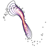
(a) curly

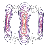
(b) 2-circles

Figure 12: Toy data land fits

(a) circle 3d

(b) circle 4d

(c) curly

(d) 2-circles

Figure 13: Boxplot error comparison (log scale, shared y-axis) of bq and mc on whole land fit for different manifolds. For mc, we allocate the runtime of the mean slowest bq method. Each box contains 16 independent runs.

Figure 14: Mean runtime comparison (for a single integration) of the bq methods. Errorbars indicate 95% confidence intervals w.r.t the 16 runs on each land fit. The reported runtimes belong to the boxplots in Fig. 13.

(a) circle 3d

(b) circle 4d

(c) curly

(d) 2-circles

Figure 15: Comparison of bq and mc errors (vertical log scale, shared legend and axes) for different manifolds, on the first integration problem of the respective land fit. Shaded regions indicate $95\%$ confidence intervals w.r.t. the $30$ independent runs.

A.4.2 mnist

We sampled $5{,}504$ random data points from the first three digits of mnist (LeCun et al., 1998), which were preprocessed by normalizing them feature-wise to $[-1,+1]$ using sklearn.preprocessing.MinMaxScaler. We trained a simple Variational-Autoencoder (VAE) to embed the $784$ dimensional input in a latent space of dimension $2$. The architecture uses separate encoders $\boldsymbol{\mathsf{\mu}}_{\phi}$, $\boldsymbol{\mathsf{\sigma}}_{\phi}$ and decoders $\boldsymbol{\mathsf{\mu}}_{\theta}$, $\boldsymbol{\mathsf{\sigma}}_{\theta}$. In summary:

Encoder/Decoder	Layer 1	Layer 2	Layer 3
$\boldsymbol{\mathsf{\mu}}_{\phi}$	128 (tanh)	64  (tanh)	2    (linear)
$\boldsymbol{\mathsf{\sigma}}_{\phi}$	128 (tanh)	64  (tanh)	2 (softplus)
$\boldsymbol{\mathsf{\mu}}_{\theta}$	64 (linear)	128 (linear)	784    (linear)
$\boldsymbol{\mathsf{\sigma}}_{\theta}$	64 (linear)	128 (linear)	784 (softplus)

We trained the network for $200$ epochs using adam with a learning rate of $10^{-3}$. The resulting latent codes were used to construct the Aggregated Posterior Metric, with $\rho=0.001$, such that the measure far from the data is $1000$. The small variances cause high curvature, which makes the integration tasks challenging and geodesic computations slow. To fit the land, we used $250$ subsampled points to lower the amount of time spent on bvps. In contrast, the gmm was fitted on the whole $5{,}504$ points. Note that Fig. 9 shows this training data.

A.4.3 adk

We obtained protein trajectory data of adenylate kinase from

https://www.mdanalysis.org/MDAnalysisData/adk_transitions.html#adk-dims-transitions-ensemble-dataset

(Seyler et al., 2015). We use the dims variant, a dataset which comprises 200 trajectories and select a subset consisting of the trajectories $160-200$, which contain in total $2{,}038$ data points. To model the assumed high curvature of the trajectory space, we choose the kernel metric with $\sigma=0.035$ and $\rho=10^{-5}$. To visualize spatial protein structure, we used the software vmd (Humphrey et al., 1996) with the “new cartoon” representation, colored according to “residue type”.

According to Seyler et al. (2015), “AdK’s closed/open transition [..] is a standard test case that captures general, essential features of conformational changes in proteins”. This well-studies transition involves the movement of the LID and NMP domains against the rather stable core domain. As a consequence, it can be described by two angles $\theta_{LID}$ and $\theta_{NMP}$. In Fig. 11, it is visible how the LID opens to the top, whereas the NMP domain moves towards the bottom right (from this particular perspective).

A.4.4 General Methodology

For the aforementioned manifolds we fitted the land mixture model with a pre-determined component number $K$.

As the ground truth, we obtained $S=40{,}000$ mc samples on each integration problem. Since obtaining a large number of exponential maps is computationally extremely expensive, we subsampled from this pool of ground truth samples when mc samples were required in the experiments, instead of running mc again. For example, in the “error vs. runtime” experiment, we calculated the mean mc runtime per sample from the ground truth pool of this particular problem and then subsampled as many samples as the given runtime limit affords. For the boxplot experiments, we averaged the mc runtimes over the whole land fit and always obtained the same number of samples per integration. Note that the mc runtime practically corresponds to the runtime of the exponential maps, since the overhead is minimal.

All experiments were run in a cloud setting on $8$ virtual CPUs. We restricted the core usage of blas linear algebra subroutines to a single core, so as not to create interference between multiple processes.

A.4.5 Manifold and Optimization Hyperparameters

In Table 2, we report the relevant hyperparameters for the metrics ($\sigma$, $\rho$), which were used to construct the manifolds, and those optimization parameters which are not equal across all problems.

Parameter	circle	circle 3d	circle 4d	circle 5d	mnist	adk	curly	2-circles
$\sigma$	0.1	0.25	0.25	0.25	-	0.035	0.2	0.15
$\rho$	0.001	0.01	0.0316	0.063	0.001	0.00001	0.01	0.01
$K$	2	2	2	2	3	1	1	3
$t_{max}$	7	4	4	4	7	7	7	7
$\alpha_{\boldsymbol{\mathsf{\mu}}}^{1}$	$0.3$	$0.3$	$0.3$	$0.3$	$0.3$	$0.2$	$0.3$	$0.3$
$\epsilon_{\nabla_{\boldsymbol{\mathsf{\mu}}}}$	$0.01$	$0.01$	$0.01$	$0.01$	$0.015$	$0.01$	$0.01$	$0.01$
integrations	67	39	40	34	105	36	33	111

Table 2: Manifold and land optimization hyperparameters and resulting number of integrations.

A.4.6 Boxplot Experiments (Fig. 5, Fig. 13)

These experiment were conducted on whole land fits, with $16$ independent runs for each of the $3$ bq methods. From Table 2, we can easily calculate the total number of runs as $48\cdot(67+39+40+34+105+36+33+111)=22{,}320$.

A.4.7 Error vs. Runtime Experiments (Fig. 7, Fig. 15)

We evenly space $30$ runtime limits between $5$ and $65$ seconds using np.linspace(5., 65., 30). For each of these runtime limits, we let each bq method run $30$ times. bq will stop collecting more samples as soon as the runtime limit is reached. After this, however, it will take some more time to finalize, as an ongoing computation is not interrupted. We then record the actually resulting runtimes and average over the 30 runs. These averages are then used for the x-axes of the plots, whereas the mean relative error is on the y-axes. In total, each bq method thus has $900$ runs on each problem. The $8$ plots, $4$ in the main paper and $4$ in the supplementary, contain $3\cdot 900\cdot 8=21{,}600$ runs. Together with the boxplot experiments, we obtain $21{,}600+22{,}=43{,}920$ bq runs, that is, $14{,}640$ for each of the $3$ methods.

In Fig. 7(c), we removed $4$ extreme dcv outliers, where seemingly the gp “broke”. This amounts to $\frac{4}{21{,}600}=0.01852\%$ of the bq runs in the $8$ plots.

References

- Amadei et al. (1993) Amadei, A., Linssen, A. B., and Berendsen, H. J. Essential dynamics of proteins. Proteins: Structure, Function, and Bioinformatics, 17(4):412–425, 1993.
- Arvanitidis et al. (2016) Arvanitidis, G., Hansen, L. K., and Hauberg, S. A Locally Adaptive Normal Distribution. In Lee, D. D., Sugiyama, M., von Luxburg, U., Guyon, I., and Garnett, R. (eds.), Advances in Neural Information Processing Systems 29: Annual Conference on Neural Information Processing Systems 2016, December 5-10, 2016, Barcelona, Spain, pp. 4251–4259, 2016.
- Arvanitidis et al. (2018) Arvanitidis, G., Hansen, L. K., and Hauberg, S. Latent space oddity: on the curvature of deep generative models. In 6th International Conference on Learning Representations, ICLR 2018, Vancouver, BC, Canada, April 30 - May 3, 2018, Conference Track Proceedings, 2018.
- Arvanitidis et al. (2019a) Arvanitidis, G., Hauberg, S., Hennig, P., and Schober, M. Fast and robust shortest paths on manifolds learned from data. In The 22nd International Conference on Artificial Intelligence and Statistics, pp. 1506–1515. PMLR, 2019a.
- Arvanitidis et al. (2019b) Arvanitidis, G., Hauberg, S., Hennig, P., and Schober, M. Fast and robust shortest paths on manifolds learned from data. In Chaudhuri, K. and Sugiyama, M. (eds.), The 22nd International Conference on Artificial Intelligence and Statistics, AISTATS 2019, 16-18 April 2019, Naha, Okinawa, Japan, volume 89 of Proceedings of Machine Learning Research, pp. 1506–1515. PMLR, 2019b.
- Arvanitidis et al. (2020) Arvanitidis, G., Hauberg, S., and Schölkopf, B. Geometrically enriched latent spaces. In arXiv preprint, 2020.
- Bhatia (2009) Bhatia, R. Positive Definite Matrices, volume 24. Princeton University Press, 2009.
- Bishop (2006) Bishop, C. M. Pattern Recognition and Machine Learning (Information Science and Statistics). Springer-Verlag, 2006.
- Briol et al. (2019) Briol, F.-X., Oates, C. J., Girolami, M., Osborne, M. A., Sejdinovic, D., et al. Probabilistic integration: A role in statistical computation? Statistical Science, 34(1):1–22, 2019.
- Chai & Garnett (2019) Chai, H. R. and Garnett, R. Improving quadrature for constrained integrands. In Chaudhuri, K. and Sugiyama, M. (eds.), The 22nd International Conference on Artificial Intelligence and Statistics, AISTATS 2019, 16-18 April 2019, Naha, Okinawa, Japan, volume 89 of Proceedings of Machine Learning Research, pp. 2751–2759. PMLR, 2019.
- Cockayne et al. (2019) Cockayne, J., Oates, C., Sullivan, T. J., and Girolami, M. Bayesian probabilistic numerical methods. SIAM Review, 61(4):756 – 789, 2019. doi: 10.1137/17M1139357.
- do Carmo (1992) do Carmo, M. P. Riemannian Geometry. Birkhäuser, 1992.
- Gessner et al. (2019) Gessner, A., Gonzalez, J., and Mahsereci, M. Active multi-information source Bayesian quadrature. In Globerson, A. and Silva, R. (eds.), Proceedings of the Thirty-Fifth Conference on Uncertainty in Artificial Intelligence, UAI 2019, Tel Aviv, Israel, July 22-25, 2019, volume 115 of Proceedings of Machine Learning Research, pp. 712–721. AUAI Press, 2019.
- Gunter et al. (2014) Gunter, T., Osborne, M. A., Garnett, R., Hennig, P., and Roberts, S. J. Sampling for inference in probabilistic models with fast Bayesian quadrature. In Ghahramani, Z., Welling, M., Cortes, C., Lawrence, N. D., and Weinberger, K. Q. (eds.), Advances in Neural Information Processing Systems 27: Annual Conference on Neural Information Processing Systems 2014, December 8-13 2014, Montreal, Quebec, Canada, pp. 2789–2797, 2014.
- Hennig & Hauberg (2014) Hennig, P. and Hauberg, S. Probabilistic solutions to differential equations and their application to Riemannian statistics. In Proceedings of the Seventeenth International Conference on Artificial Intelligence and Statistics, AISTATS 2014, Reykjavik, Iceland, April 22-25, 2014, volume 33 of JMLR Workshop and Conference Proceedings, pp. 347–355. JMLR.org, 2014.
- Hennig et al. (2015) Hennig, P., Osborne, M. A., and Girolami, M. Probabilistic numerics and uncertainty in computations. Proceedings of the Royal Society of London A: Mathematical, Physical and Engineering Sciences, 2015.
- Humphrey et al. (1996) Humphrey, W., Dalke, A., and Schulten, K. VMD – Visual Molecular Dynamics. Journal of Molecular Graphics, 14:33–38, 1996.
- Kanagawa & Hennig (2019) Kanagawa, M. and Hennig, P. Convergence guarantees for adaptive Bayesian quadrature methods. In Wallach, H. M., Larochelle, H., Beygelzimer, A., d’Alché-Buc, F., Fox, E. B., and Garnett, R. (eds.), Advances in Neural Information Processing Systems 32: Annual Conference on Neural Information Processing Systems 2019, NeurIPS 2019, December 8-14, 2019, Vancouver, BC, Canada, pp. 6234–6245, 2019.
- Kingma & Welling (2014) Kingma, D. P. and Welling, M. Auto-encoding variational Bayes. In Bengio, Y. and LeCun, Y. (eds.), 2nd International Conference on Learning Representations, ICLR 2014, Banff, AB, Canada, April 14-16, 2014, Conference Track Proceedings, 2014.
- LeCun et al. (1998) LeCun, Y., Bottou, L., Bengio, Y., and Haffner, P. Gradient-based learning applied to document recognition. Proceedings of the IEEE, 86(11):2278–2324, 1998. doi: 10.1109/5.726791.
- Lee (2018) Lee, J. Introduction to Riemannian Manifolds. Springer, 2018.
- O’Hagan (1991) O’Hagan, A. Bayes–Hermite quadrature. Journal of Statistical Planning and Inference, 29(3):245–260, 1991.
- Papaleo et al. (2009) Papaleo, E., Mereghetti, P., Fantucci, P., Grandori, R., and De Gioia, L. Free-energy landscape, principal component analysis, and structural clustering to identify representative conformations from molecular dynamics simulations: the Myoglobin case. Journal of Molecular Graphics and Modelling, 27(8):889–899, 2009.
- Pennec (2006) Pennec, X. Intrinsic statistics on Riemannian manifolds: Basic tools for geometric measurements. Journal of Mathematical Imaging and Vision, 25(1):127, 2006.
- Rasmussen & Williams (2006) Rasmussen, C. E. and Williams, C. K. Gaussian Processes for Machine Learning, volume 2. MIT press Cambridge, MA, 2006.
- Rezende et al. (2014) Rezende, D. J., Mohamed, S., and Wierstra, D. Stochastic backpropagation and approximate inference in deep generative models. In Proceedings of the 31th International Conference on Machine Learning, ICML 2014, Beijing, China, 21-26 June 2014, volume 32 of JMLR Workshop and Conference Proceedings, pp. 1278–1286. JMLR.org, 2014.
- Seyler et al. (2015) Seyler, S. L., Kumar, A., Thorpe, M. F., and Beckstein, O. Path similarity analysis: A method for quantifying macromolecular pathways. PLOS Computational Biology, 11(10):1–37, 10 2015. doi: 10.1371/journal.pcbi.1004568. URL https://doi.org/10.1371/journal.pcbi.1004568.
- Spellmon et al. (2015) Spellmon, N., Sun, X., Sirinupong, N., Edwards, B., Li, C., and Yang, Z. Molecular dynamics simulation reveals correlated inter-lobe motion in protein Lysine Methyltransferase SMYD2. PLOS ONE, 10(12):e0145758, 2015.
- Stein (2012) Stein, M. L. Interpolation of spatial data: some theory for kriging. Springer Science & Business Media, 2012.
- Tosi et al. (2014) Tosi, A., Hauberg, S., Vellido, A., and Lawrence, N. D. Metrics for probabilistic geometries. In Zhang, N. L. and Tian, J. (eds.), Proceedings of the Thirtieth Conference on Uncertainty in Artificial Intelligence, UAI 2014, Quebec City, Quebec, Canada, July 23-27, 2014, pp. 800–808. AUAI Press, 2014.
- Townsend et al. (2016) Townsend, J., Koep, N., and Weichwald, S. Pymanopt: A python toolbox for optimization on manifolds using automatic differentiation. The Journal of Machine Learning Research, 17(1):4755–4759, 2016.
- Tribello & Gasparotto (2019) Tribello, G. A. and Gasparotto, P. Using dimensionality reduction to analyze protein trajectories. Frontiers in Molecular Biosciences, 6:46, 2019. ISSN 2296-889X. doi: 10.3389/fmolb.2019.00046.
- Wagstaff et al. (2018) Wagstaff, E., Hamid, S., and Osborne, M. Batch selection for parallelisation of Bayesian quadrature. arXiv preprint arXiv:1812.01553, 2018.
- Wolf & Kirschner (2013) Wolf, A. and Kirschner, K. N. Principal component and clustering analysis on molecular dynamics data of the ribosomal l11· 23s subdomain. Journal of Molecular Modeling, 19(2):539–549, 2013.
- Xi et al. (2018) Xi, X., Briol, F., and Girolami, M. A. Bayesian quadrature for multiple related integrals. In Dy, J. G. and Krause, A. (eds.), Proceedings of the 35th International Conference on Machine Learning, ICML 2018, Stockholmsmässan, Stockholm, Sweden, July 10-15, 2018, volume 80 of Proceedings of Machine Learning Research, pp. 5369–5378. PMLR, 2018.