Extending superposed harmonic initial data to higher spin

Abstract

Numerical simulations of binary black holes are accompanied by an initial spurious burst of gravitational radiation (called ‘junk radiation’) caused by a failure of the initial data to describe a snapshot of an inspiral that started at an infinite time in the past. A previous study showed that the superposed harmonic (SH) initial data gives rise to significantly smaller junk radiation. However, it is difficult to construct SH initial data for black holes with dimensionless spin $\chi\gtrsim 0.7$. We here provide a class of spatial coordinate transformations that extend SH to higher spin. The new spatial coordinate system, which we refer to as superposed modified harmonic (SMH), is characterized by a continuous parameter — Kerr-Schild and harmonic spatial coordinates are only two special cases of this new gauge. We compare SMH with the superposed Kerr-Schild (SKS) initial data by evolving several binary black hole systems with $\chi=0.8$ and $0.9$. We find that the new initial data still leads to less junk radiation and only small changes of black hole parameters (e.g. mass and spin). We also find that the volume-weighted constraint violations for the new initial data converge with resolution during the junk stage $(t\lesssim 700M)$, which means there are fewer high-frequency components in waveforms at outer regions.

I Introduction

The detection of GW150914 Abbott et al. (2016) and other binary compact objects Abbott et al. (2019, 2020); 190 (a, b, c) has opened a new era in astrophysics. With the improvement of detector sensitivity, more and more events are expected to be detected in the near future Abadie et al. (2010). Therefore, an accurate modeling of coalescing binaries is crucial for data analysis. Numerical relativity (NR) remains the only ab initio method to simulate the coalescence of binary black hole (BBH) systems. With NR, one can obtain the entire BBH waveform including inspiral, merger, and ringdown. Moreover, gravitational wave models Varma et al. (2019a, b); Ossokine et al. (2020); Cotesta et al. (2018); Bohé et al. (2017); Pratten et al. (2020a); García-Quirós et al. (2020); Pratten et al. (2020b) used to analyze detector data are ultimately calibrated against NR.

Numerical simulations of BBHs are based on splitting the Einstein equation into constraint and evolution parts, where the constraint equations provide the initial data to evolve. However, the constructed initial data does not exactly correspond to a quasi-equilibrium state of an inspiral that started at an infinite time in the past. For example, the tidal distortion of a BH is not fully recovered, and the initial data do not usually include gravitational radiation already present. As a result, once the evolution begins, the system relaxes into a quasi-equilibrium state, and gives rise to a pulse of spurious radiation, which is referred to as ‘junk radiation’. Several attempts have been made to reduce junk radiation, by introducing PN corrections Alvi (2000); Yunes and Tichy (2006); Johnson-McDaniel et al. (2009); Kelly et al. (2010); Reifenberger and Tichy (2012); Tichy (2017), or by using a curved conformal metric Lovelace (2009); Johnson-McDaniel et al. (2009); Varma et al. (2018).

Recently, Varma et al. Varma et al. (2018) carried out a systematic study of initial data and its effects on junk radiation and computational efficiency of the subsequent time evolution. The simulations studied in Varma et al. were performed with an NR code: the Spectral Einstein Code (SpEC) spe , where the construction of initial data is based on the Extended Conformal Thin Sandwich (XCTS) formulation York (1999); Pfeiffer and York (2003). Within this formalism, several free fields, including the conformal metric, must be provided. Different choices of the free fields generate different physical initial data; the data still correspond to two black holes with the same desired mass ratio and spins, but the initial tidal distortions and strong-field dynamics differ. Varma et al. showed that the junk radiation and efficiency of the subsequent evolution depend on the given free fields. In particular, choosing the initial data based on two superposed black holes in time-independent harmonic coordinates Cook and Scheel (1997) (heretofore called superposed harmonic (SH) data) leads to less junk radiation than superposed Kerr-Schild (SKS) initial data Lovelace (2009), which is typically used in SpEC simulations Boyle et al. (2019). Varma et al. also found that SH initial data has higher computational efficiency. However, SH initial data works well only for BHs with dimensionless spin $\chi\lesssim 0.7$. For high-spin BHs, the horizons become so highly deformed that it is difficult to construct initial data (cf. Fig. 10 in Ref. Varma et al. (2018)).

For both SH and SKS initial data, the conformal spatial metric and the trace of the extrinsic curvature are determined by superposing the analytic solutions for two single Kerr black holes. The difference is that SKS uses the Kerr metric in Kerr-Schild coordinates, and SH uses the Kerr metric in time-independent harmonic coordinates Cook and Scheel (1997). It may be surprising that making a different coordinate choice — the choice of coordinates for the single-BH analytic solution — leads to a different physical BBH solution. The reason is that the superposition of two single-BH solutions does not solve the Einstein equations for a BBH and is used to compute only some of the fields; the remaining fields are computed by solving constraints and by quasi-equilibrium conditions. For a single black hole, following the complete initial data procedure (including solving the constraints numerically) for both SKS and SH would result in the same physical Kerr metric but in different coordinates.

In this paper, we extend SH to higher spins by using a spatial coordinate map to transform the free data for the single-BH conformal metric, while retaining harmonic time slicing for this single-BH conformal metric. The coordinate transformation defines a class of spatial coordinate systems that are characterized by a continuous parameter $\alpha$. We refer to these coordinates as the modified harmonic (MH) coordinate system. MH coordinates are purely harmonic with $\alpha=1$ and correspond to spatial KS when $\alpha=0$. Similar to the cases of SKS and SH, an initial data for a BBH system can also be constructed by superposing two single Kerr black holes in MH coordinates. We refer to this initial data as superposed modified harmonic (SMH). For the BBH systems with $\chi>0.7$, a value of $\alpha<1$ results in less distorted horizons. However, it is desirable to keep $\alpha$ as close to 1 as possible so that SMH data still shares the desirable properties of SH initial data.

This paper is organized as follows. In Sec. II, we provide some basic information about how we compute initial data and evolve BBH systems. In Sec. III, we compare the behavior of different single-BH coordinate systems. In particular, in Sec. III.5 we explicitly point out the numerical reason that SH does not work for high-spin BHs. This immediately leads to a class of spatial coordinate transformations, defined in Sec. III.6, that can cure the numerical issues. We then use the MH coordinate system to construct initial data for BBHs (i.e., SMH) with $\chi=0.8$ and $0.9$ and evolve these systems. In Sec. IV, we discuss the results of our simulations. Finally in Sec. V, we discuss our results and highlight possible future work.

Throughout the paper, we use Latin letters to stand for the spatial indices, and use Greek letters to represent spacetime indices.

II BBH initial data and evolution

Following the discussions in Ref. Varma et al. (2018), we use the XCTS formulation to construct initial data for a binary black hole system. Within this formalism, one can freely specify the conformal metric $\bar{g}_{ij}$, trace of extrinsic curvature $K$, and their time derivatives $\partial_{t}\bar{g}_{ij}$ and $\partial_{t}K$. To obtain quasi-equilibrium initial data, we choose

$$\partial_{t}\bar{g}_{ij}=0,\quad\partial_{t}K=0\,.$$ (1)

The construction of the other free fields, $\bar{g}_{ij}$ and $K$, is based on the 3-metric $g_{ij}^{\beta}$ and the trace of extrinsic curvature $K^{\beta}$ of two single boosted Kerr BHs , where the superscript $\beta=1,2$ labels each of the two BHs in the binary system. The conformal metric and the trace of the extrinsic curvature are then given by:

$$\bar{g}_{ij}=f_{ij}+\sum_{\beta=1}^{2}e^{-r_{\beta}^{2}/w_{\beta}^{2}}(g_{ij}^{\beta}-f_{ij}),$$ (2)

$$K=\sum_{\beta=1}^{2}e^{-r_{\beta}^{2}/w_{\beta}^{2}}K^{\beta}\,,$$ (3)

where $f_{ij}$ is the flat 3-metric, and $r_{\beta}$ is the Euclidean coordinate distance from the center of each BH Lovelace et al. (2008). Note that each metric is weighted by a Gaussian with width

$$w_{\beta}=0.6\,d_{\beta}^{L_{1}}\,,$$ (4)

where $d_{\beta}^{L_{1}}$ is the Euclidean distance between the Newtonian $L_{1}$ Lagrange point and the center of the black hole labeled by $\beta$. Here $g_{ij}^{\beta}$ and $K^{\beta}$ correspond to the Kerr solution expressed either in the KS, harmonic, or MH coordinate systems. BBH initial data constructed from the two Kerr solutions in the aforementioned coordinates are referred to as SKS, SH, and superposed modified harmonic (SMH), respectively.

After specifying the free fields, the initial data are completed by solving a set of coupled elliptic equations that ensure satisfaction of the constraints and an additional quasi-equilibrium condition. Additionally, these elliptic equations require boundary conditions. At the outer boundary (typically chosen to be $10^{9}\,M$ from the sources), we impose asymptotic flatness [cf. Eq. (11)—(13) in Ref. Varma et al. (2018)], and at each inner boundary we enforce an apparent horizon condition [cf. Eq. (15)—(24) in Ref. Varma et al. (2018)]. After generating initial data in the XCTS formalism, we also need to specify the initial gauge for time evolution. Here we use the most common choice for SpEC simulations: $\partial_{t}N=\partial_{t}N^{i}=0$ in a corotating frame, where $N$ is the lapse function and $N^{i}$ is the shift vector. It was shown that the damped harmonic gauge Szilagyi et al. (2009) is the most suitable for mergers, so we do a smooth gauge transformation on a time scale of $\sim 50\,M$ during the early inspiral, to transform from the initial gauge to the better suited damped harmonic gauge.

III Modified harmonic coordinate system

In this section, we aim to investigate the reason that makes the harmonic coordinates problematic for high-spin BHs. We begin with a brief review of KS coordinates in Sec. III.1. Then in Sec. III.2, we outline a method that can be used to study the numerical behavior of Kerr metric in different coordinate systems. It is then applied to KS spatial coordinates with harmonic slicing in Sec. III.3, and to harmonic coordinates in Sec. III.4. Those analyses allow us to explicitly show the numerical problem with using harmonic coordinates for high-spin BHs, as discussed in Sec. III.5. Finally in Sec. III.6, we provide a coordinate map to fix the problem.

III.1 Kerr in Kerr-Schild coordinates

For a stationary Kerr BH with mass $M$ and angular momentum $\chi M^{2}$ in the $z$ direction, the metric in KS coordinates $x^{\mu}_{\text{KS}}=(t_{\text{KS}},x_{\text{KS}},y_{\text{KS}},z_{\text{KS}})$ is given by Kerr (1963)

$$ds^{2}=g_{\mu\nu}dx^{\mu}_{\text{KS}}dx^{\nu}_{\text{KS}}=(\eta_{\mu\nu}+2Hl_{\mu}l_{\nu})dx^{\mu}_{\text{KS}}dx^{\nu}_{\text{KS}}\,,$$ (5)

where $\eta_{\mu\nu}$ is the Minkowski metric, $H$ is a scalar function, and $l_{\mu}$ is a null covariant vector. The expressions for $H$ and $l_{\mu}$ are not used here but can be found in Ref. Kerr (1963). With KS coordinates, the radial Boyer-Lindquist coordinate $r$ can be written as Kerr (1963)

$$r^{2}=\frac{1}{2}(x_{\text{KS}}^{2}+y_{\text{KS}}^{2}+z_{\text{KS}}^{2}-a^{2})$$

$$+\left[\frac{1}{4}(x_{\text{KS}}^{2}+y_{\text{KS}}^{2}+z_{\text{KS}}^{2}-a^{2})^{2}+a^{2}z_{\text{KS}}^{2}\right]^{1/2}\,,$$ (6)

or equivalently

$$\frac{x_{\text{KS}}^{2}+y_{\text{KS}}^{2}}{r^{2}+a^{2}}+\frac{z_{\text{KS}}^{2}}{r^{2}}=1\,.$$ (7)

Here we have used $a=\chi M$ for the sake of conciseness. The outer and inner horizons of the BH are located at

$$r_{\pm}=M\pm\sqrt{M^{2}-a^{2}}\,.$$ (8)

III.2 Transforming from KS to a different coordinate system

Now we introduce a new coordinate system $x^{\mu}=(t,x,y,z)$, which are related to the KS coordinates $x^{\mu}_{\text{KS}}$ through

$$\left(\begin{matrix}dt_{\text{KS}}\\ dx_{\text{KS}}\\ dy_{\text{KS}}\\ dz_{\text{KS}}\end{matrix}\right)=\left(\begin{matrix}1&\bm{b}\\ \bm{0}&\bm{C}\end{matrix}\right)\left(\begin{matrix}dt\\ dx\\ dy\\ dz\end{matrix}\right)\,,$$ (9)

where $\bm{b}$ is a 3D vector, and $\bm{C}$ is a $3\times 3$ matrix. In Eq. (9), we have assumed that the new spatial coordinates are independent of $t_{\text{KS}}$. Note that we here keep the forms of $\bm{b}$ and $\bm{C}$ generic, so that our present discussion can be applied to different coordinate systems.

With the Jacobian at hand, we could transform the Kerr metric into the new coordinates, and study the numerical features of each metric component, such as the problematic behavior of harmonic coordinates for high-spin black holes, but this usually involves very complicated calculations. However, since $g_{\mu\nu}^{\text{KS}}$ can be decomposed into two pieces [Eq. (5)], it is simpler to study the transformations of $\eta_{\mu\nu}$. In the new coordinates, we have

$$\eta_{\mu\nu}= \left(\begin{matrix}-1&\bm{0}\\ \bm{0}&\mathbb{I}^{3}\end{matrix}\right)\rightarrow\left(\begin{matrix}1&\bm{b}\\ \bm{0}&\bm{C}\end{matrix}\right)^{T}\left(\begin{matrix}-1&\bm{0}\\ \bm{0}&\mathbb{I}^{3}\end{matrix}\right)\left(\begin{matrix}1&\bm{b}\\ \bm{0}&\bm{C}\end{matrix}\right)$$

$$=\left(\begin{matrix}-1&-\bm{b}\\ -\bm{b}^{T}&\bm{C}^{T}\bm{C}-\bm{b}^{T}\bm{b}\end{matrix}\right)\,,$$ (10)

where $\mathbb{I}^{3}$ is the three-dimensional identity matrix. Both the 3-metric $(\bm{C}^{T}\bm{C}-\bm{b}^{T}\bm{b})$ and the shift vector $-\bm{b}$ above are modified by the vector $\bm{b}$. Any numerically problematic term in $\bm{b}$ might cause difficulty to resolve the metric in the new coordinates. Below, we focus on the $z$ component of $\bm{b}$, $b^{z}$, at the inner boundary $r=r_{+}$, and study its numerical behavior for high-spin black holes (especially when $a\to M$) with several coordinates.

III.3 Kerr-Schild spatial coordinates with harmonic slicing

We first apply our discussion in Sec. III.2 to a mixed coordinate system: KS spatial coordinates together with harmonic temporal slicing, then we have

$$\bm{C}_{\text{KSHS}}=\mathbb{I}^{3},$$ (11a)

$$\bm{b}_{\text{KSHS}}=\frac{2M}{r-r_{-}}\bm{\nabla}r,$$ (11b)

where the subscript ‘KSHS’ stands for Kerr-Schild spatial coordinates with Harmonic Slicing; and $r$ is the radial Boyer-Lindquist coordinate. Note that Eq. (11b) is the result of Cook and Scheel (1997)

$$t_{\text{KSHS}}=t_{\text{KS}}-\int\frac{2M}{r-r_{-}}\,dr\,.$$ (12)

We refer the reader to Appendix A for the detailed expression of $\bm{\nabla}r$. The $z$ component of $\bm{b}_{\text{KSHS}}$ at the inner boundary $r=r_{+}$ is given by (as $a\to M$)

$$b^{z}_{\text{KSHS}}=\frac{M^{2}z_{\text{KS}}}{r_{+}^{4}+(az_{\text{KS}})^{2}}\,.$$ (13)

III.4 Harmonic coordinates

Let us turn our attention to harmonic coordinates $x^{\mu}_{\text{H}}=(t_{\text{H}},x_{\text{H}},y_{\text{H}},z_{\text{H}})$, where the spatial coordinates also become harmonic. For such a coordinate system, we have Cook and Scheel (1997)

$$(r-M)^{2}=\frac{1}{2}(x_{\text{H}}^{2}+y_{\text{H}}^{2}+z_{\text{H}}^{2}-a^{2})$$

$$+\left[\frac{1}{4}(x_{\text{H}}^{2}+y_{\text{H}}^{2}+z_{\text{H}}^{2}-a^{2})^{2}+a^{2}z_{\text{H}}^{2}\right]^{1/2}\,,$$ (14)

and

$$\frac{x_{\text{H}}^{2}+y_{\text{H}}^{2}}{(r-M)^{2}+a^{2}}+\frac{z_{\text{H}}^{2}}{(r-M)^{2}}=1\,,$$ (15)

where the subscript ‘H’ stands for harmonic coordinates. The harmonic slicing implies

$$\bm{b}_{\text{H}}=\frac{2M}{r-r_{-}}\bm{\nabla}r,$$ (16)

with $z$ component of $\bm{b}_{\text{H}}$ at $r=r_{+}$ given by (as $a\to M$)

$$b_{\text{H}}^{z}=\frac{M^{2}z_{\text{H}}}{(r_{+}-M)^{4}+(az_{\text{H}})^{2}}\,.$$ (17)

Expressions for the $3\times 3$ block matrix, $(C_{\text{H}})^{i}_{j}=\partial x_{\text{KS}}^{i}/\partial x_{\text{H}}^{j}$ , along with additional details, can be found in Appendix A.

III.5 Problematic behavior of harmonic coordinates

In SpEC, the Legendre polynomials are used to numerically expand $b_{\text{H}}^{z}$ and $b_{\text{KSHS}}^{z}$ as functions of $\cos\theta$, defined by

$$\cos\theta=\frac{z_{\text{H}}}{\sqrt{x^{2}_{\text{H}}+y^{2}_{\text{H}}+z^{2}_{\text{H}}}}\,.$$

Here $\theta$ is the polar angle in harmonic coordinates and is not to be confused with the angular Boyer-Lindquist coordinate. As a test, we first represent $b_{\text{H}}^{z}$ [Eq. (17)] with twenty Legendre-Gauss collocation points and a BH spin of $a=0.95\,M$. The results of this test are shown in Fig. 1. From Fig. 1, we see that the function $b_{\text{H}}^{z}$ is difficult to resolve using Legendre polynomials. This is the primary reason that harmonic coordinates fail to accurately represent high-spin BH initial data. Note that increasing the resolution to $l\gtrsim 60$ (for a single BH) eventually allows us to resolve $b_{\text{H}}^{z}$, but in practice requiring such high resolution is computationally prohibitive; furthermore, the required resolution increases rapidly as the spin increases.

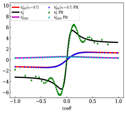
Figure 1: The function $b^{z}$ in KSHS [Eq. (13)], harmonic [Eq. (17)] and MH [Eq. (23)] coordinates with $\alpha=0.7$. Solid lines represent $b^{z}$, whereas triangles represent the Legendre-Gauss collocation approximation to each function $b^{z}$ using $20$ Legendre polynomials. The spin of the BH is $a=0.95\,M$. $b^{z}$ is better approximated by a fixed number ($l=20$) of Legendre polynomials for MH than for harmonic coordinates.

Previous studies have shown success in high-spin BBH simulations with SKS initial data up to spins of $\chi=0.998$ Scheel et al. (2015). A natural question to ask is whether the spatial or the time coordinates are more important in allowing KS coordinates to better resolve highly-spinning black holes. Therefore, we also investigate the behavior of $b^{z}_{\text{KSHS}}$ (see Sec. III.3) in which the time coordinate is harmonic but the spatial coordinates are Kerr-Schild. Again, we represent $b^{z}_{\text{KSHS}}$ with twenty Legendre-Gauss collocation points and a BH spin of $a=0.95M$, as shown in Fig. 1. The representation is much better than the case of harmonic coordinates. And we also confirm that with such mixed coordinates, BBH initial data can be indeed extended to higher spins. However, as we show later, they do not lead to a smaller amount of junk radiation than SKS initial data.

Looking more closely at Fig. 1, $b^{z}_{\text{KSHS}}$ has fewer structures than $b_{\text{H}}^{z}$, which makes $b^{z}_{\text{KSHS}}$ easier to represent by Legendre polynomials. More quantitatively, we write

$$b_{\text{H}}^{z}\sim\frac{1}{u^{2}+\frac{\epsilon}{1+\epsilon}},$$ (18)

with

$$u=\frac{a}{r_{+}-M}\cos\theta,\quad\epsilon=\frac{(r_{+}-M)^{2}}{(r_{+}-M)^{2}+a^{2}}.$$ (19)

In Eq. (18), we have omitted unimportant functions of $\cos\theta$ since they are well represented by Legendre polynomials. We see $b_{\text{H}}^{z}$ has two poles $u=\pm i\sqrt{\epsilon/(1+\epsilon)}$. The domain of convergence for Legendre series $P_{n}(\cos\theta)$ is an elliptic region on the complex plane Boyd (2001). If we restrict ourselves to the real axis, we can obtain the radius of convergence as

$$|\cos\theta|\lesssim\sqrt{\frac{1+2\epsilon}{1+\epsilon}}\frac{r_{+}-M}{a}.$$ (20)

The radius becomes less than 1 if $a\gtrsim 0.75M$, thus in that case the Legendre polynomials fail to provide a good representation for the metric. This is the main reason that BBH simulations using SH become difficult when spins are larger than about $a=0.7M$ Varma et al. (2018). We remark that Chebyshev series have the same domain of convergence as Legendre series; hence we do not expect the situation can be improved by changing basis.

III.6 Modified Harmonic coordinates

We have seen that $b^{z}_{\text{H}}$ is sensitive to $\cos\theta$ for high-spin BHs. To reduce such dependence, we define a more general coordinate system

$$\frac{x_{\text{MH}}^{2}+y_{\text{MH}}^{2}}{(r-\alpha M)^{2}+a^{2}}+\frac{z_{\text{MH}}^{2}}{(r-\alpha M)^{2}}=1,\quad t_{\text{MH}}=t_{\text{H}}\,,$$ (21)

which leads to

$$(r-\alpha M)^{2}=\frac{1}{2}(x_{\text{MH}}^{2}+y_{\text{MH}}^{2}+z_{\text{MH}}^{2}-a^{2})$$

$$+\left[\frac{1}{4}(x_{\text{MH}}^{2}+y_{\text{MH}}^{2}+z_{\text{MH}}^{2}-a^{2})^{2}+a^{2}z_{\text{MH}}^{2}\right]^{1/2}\,.$$ (22)

Here we introduce a new constant parameter $\alpha$. As mentioned earlier, we refer to this new choice of spatial coordinates as the modified harmonic (MH) coordinate system. MH coordinates become harmonic (spatial) coordinates when $\alpha=1$ [Eq. (15)] and become KS (spatial) coordinates when $\alpha=0$ [Eq. (7)]. Meanwhile, the time slicing of MH coordinates is the same as in harmonic, regardless of the value of $\alpha$. With this new coordinate system, the radius of the outer horizon along the spin direction is $(1-\alpha)M+\sqrt{M^{2}-a^{2}}$. For $a\to M$, this radius goes to $M$ for KS coordinates ($\alpha=0$) and it goes to zero for harmonic coordinates ($\alpha=1$). Therefore, the horizon with harmonic coordinates is highly compressed in the spin direction. However, if we let $\alpha$ be a number smaller than, but still close to 1, the horizon will be less distorted. On the other hand, since $\alpha$ is close to 1, we can expect that it still shares some similar properties (e.g. less junk radiation) with harmonic coordinates.

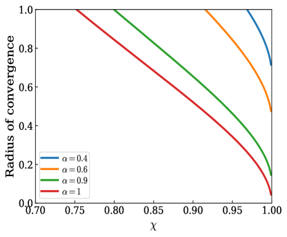
Figure 2: The radius of convergence given in Eq. (25).

As in Sec. III.5, we use the function $b^{z}$ as an example to see the improvement offered by MH coordinates. In the MH coordinate system, we have

$$b^{z}_{\text{MH}}=\frac{M^{2}z_{\text{MH}}}{(r_{+}-\alpha M)^{4}+(az_{\text{MH}})^{2}}\,.$$ (23)

Now $(r_{+}-M)^{2}$ is replaced by $(r_{+}-\alpha M)^{2}$. The problematic part of $b^{z}_{\text{MH}}$ takes the same form as Eq. (18), except that

$$u=\frac{a}{r_{+}-\alpha M}\cos\theta,\quad\epsilon=\frac{(r_{+}-\alpha M)^{2}}{(r_{+}-\alpha M)^{2}+a^{2}}.$$ (24)

And the radius of convergence is given by

$$|\cos\theta|\lesssim\sqrt{\frac{1+2\epsilon}{1+\epsilon}}\frac{r_{+}-\alpha M}{a}.$$ (25)

In Fig. 2, we plot the radius of convergence as a function of $\chi=a/M$ for several values of $\alpha$. We see the convergent region for a fixed $\chi$ is enlarged if $\alpha$ becomes smaller. As a consequence, it should be easier for Legendre polynomials to represent $b^{z}_{\text{MH}}$. To see that this is the case, in Fig. 2 we plot $b^{z}_{\text{MH}}$ with $\alpha=0.7$ and $a=0.95\,M$, using the same set of angular Legendre-Gauss collocation points as for the other curves in the figure. As expected, the representation in Legendre polynomials of $b^{z}_{\text{MH}}$ shows an enormous improvement over the same representation of $b^{z}_{\text{H}}$.

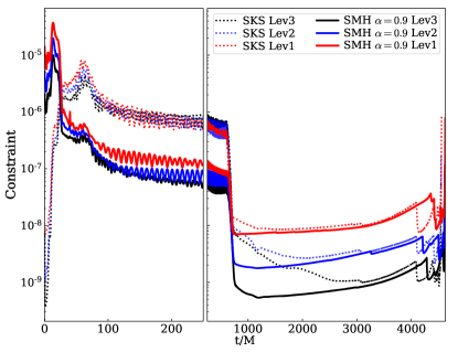
Figure 3: The volume-weighted generalized harmonic constraint energy for evolutions of Case I, with both SKS (dotted lines) and SMH (solid lines) initial data. Three resolutions are shown, labeled ’Lev1’ (red), ’Lev2’ (blue), and ’Lev3’ (black) in order of decreasing AMR tolerance (i.e. in order of increasing numerical resolution). At the beginning, BHs of SMH initial data are more distorted on the grid so the constraints are worse. However, as the gauge transition proceeds, the constraints decay quickly. During most of the junk stage $(25M\lesssim t\lesssim 700M)$, the constraints of SMH initial data are smaller than SKS by an order of magnitude. They also converge with resolution. After the junk stage, SKS and SMH finally become comparable.

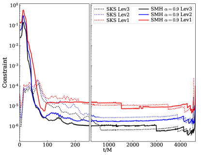
Figure 4: Same as Fig. 3, except that $L^{2}$ norm is used.

IV Results

In this section we investigate the numerical behavior of BBHs evolved starting with SMH initial data, compared to evolution of SKS data. We pick four cases, as summarized in Table 1. To make comparisons, we consider constraint violations, computational efficiency, changes of BH parameters (mass and spin), and junk radiation. For the first three factors, we show the general features of SMH by focusing on Case I. For junk radiation, we study all cases. For each simulation, we evolve with three resolutions (labeled Lev 1,2,3 in order of increasing resolution). The resolution is chosen by specifying different numerical error tolerances to the adaptive mesh refinement (AMR) algorithm Szilágyi (2014). The orbital eccentricity is iteratively reduced to below $\sim 10^{-3}$ Buonanno et al. (2011). The coordinate sizes of the black holes are different for SMH and SKS, so the excision boundaries (which are placed just inside each apparent horizon) are also different for SMH and SKS; this means that the grids are not exactly the same beween the two cases, but the grid points are chosen by AMR so that the two cases have the same approximate numerical error.

Table 1: A summary of parameters (mass ratio $q$ and dimensionless spins $\bm{\chi}$) for four simulations, where the spins of Case II are chosen randomly. The orbital angular momentum is pointing along $(0,0,1)$. In the final column, we show the value of $\alpha$ for MH coordinates.

Simulation label	$q$	$\bm{\chi}_{1}$	$\bm{\chi}_{2}$	$\alpha$
Case I	1	$(0,0,0.8)$	$(0,0,0.8)$	0.9
Case II	1	$(0.44,0.44,0.50)$	$(0.13,0.64,0.46)$	0.9
Case III	2	$(0,0,0.7)$	$(0,0,0.8)$	0.8
Case IV	1	$(0,0,0.9)$	$(0,0,0.9)$	0.7

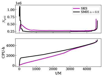
Figure 5: Computational efficiency of evolutions of SMH $(\alpha=0.9)$ and SKS initial data for Case I, with the highest resolution. The upper panel is the total number of grid points as a function of time. At the beginning, the SMH initial data requires many more grid points to meet the error tolerance. As the gauge transition to damped harmonic gauge proceeds (on a time scale of $\sim 50\,M$), the BHs become less distorted, so AMR gradually drops points. At the same time, several concentric spherical shells around each of the BHs are dropped, which leads to discontinuous jumps in the number of grid points. In the end, evolutions of SMH initial data has fewer collocation points than for SKS. The lower panel is the accumulated CPU hours versus time. The SMH initial data is extremely slow at the beginning. As the collocation points and subdomains are adjusted, it speeds up. The total CPU hours for evolutions of both initial data sets are similar.

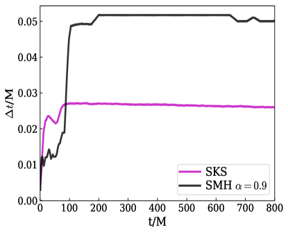
Figure 6: The time step as a function of evolution time. The resolution is Lev 3. Initially, the time step for evolutions of SKS initial data is larger than for SMH. However, after several jumps due to the shell-dropping algorithm, SMH eventually has a larger time step than SKS.

IV.1 Constraint violations and computational efficiency

Figure 3 shows the evolution of the volume-weighted generalized harmonic constraint energy $N_{\mathrm{volume}}$, which is given by [Eq. (53) of Ref. Lindblom et al. (2006)]

$$N_{\mathrm{volume}}=\sqrt{\frac{\int_{V}F(x)^{2}d^{3}x}{\int_{V}d^{3}x}},$$ (26)

with $F(x)$ the generalized harmonic constraint energy at $x$. For the first $\sim 25\,M$ of evolution, the constraints of SMH are much larger than those of SKS. This is because BHs with SMH initial data are more distorted than SKS, and the metric is more difficult to resolve; however, the metric is much easier to resolve for SMH than SH (which is not shown because even constructing the initial data for SH is problematic with a spin of $\chi=0.8$). Furthermore, at slightly later times, constraints decrease rapidly. During the junk stage ($t\lesssim 700\,M$), the constraints for the evolution of SMH initial data are smaller than those of SKS by an order of magnitude. After the junk leaves the system, the evolution of SMH initial data is still a little bit better than that of SKS initial data, although constraints of SKS and SMH become similar at late times ($t\gtrsim 3000\,M$ for Lev 3 and $t\gtrsim 2000\,M$ for Lev 2).

During the junk stage we make no attempt to resolve the junk oscillations, i.e., the AMR algorithm is intentionally set to change the grid very infrequently (and not at all in the wave zone) during the junk stage of the evolution. We do this because resolving junk is computationally expensive and because the junk is not part of the physical solution we care about. Accordingly, the SKS curves in Figure 3 are not well-resolved during the junk stage and do not show good convergence. However, we notice that the simulations of SMH initial data are better resolved than for SKS, and they converge with resolution even during the junk stage; convergence during the junk stage was also observed for SH with low-spin BHs Varma et al. (2018).

The convergence plot looks slightly different when the norm of the constraint energy is determined using a pointwise $L^{2}$ norm over grid points rather than an integral over the volume, as given by

$$N_{\mathrm{pointwise}}=\sqrt{\frac{\sum\limits_{i=1}^{N}(F_{i})^{2}}{N}},$$ (27)

where the subscript $i$ stands for the index of a grid point, and $N$ is the total number of grid points. The pointwise norm is shown in Fig.4. For the pointwise norm the improvement of convergence of SMH over SKS is not as good as for the volume-weighted norm. This is because the pointwise norm gives larger weight to the interior regions near the BHs where there are more points, whereas the volume norm gives larger weight to the exterior wave zone which covers more volume. The difference beween Figs. 3 and 4 illustrates that the improvement of the constraints in the case of SMH mainly comes from the outer region, where the high-frequency components in the waveforms are smaller (i.e., less junk radiation). Figure 4 also shows that the pointwise norms ($L^{2}$ norm) for evolutions of both initial data sets become comparable much earlier than the volume norms ($t\sim 200\,M$). This is because the pointwise norms are monitored by AMR, and therefore their values remain consistent with the numerical error tolerance in AMR during the evolution as AMR makes changes to the grid resolution.

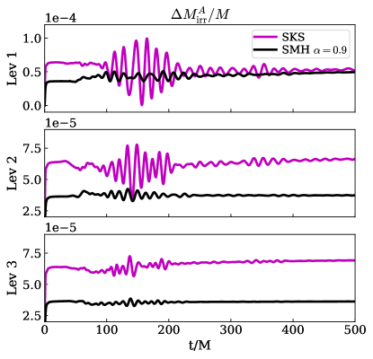
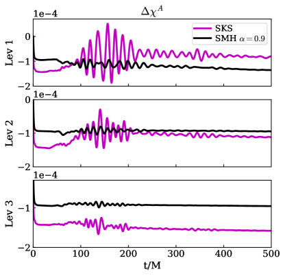
Figure 7: The evolution of irreducible mass (left) and dimensionless spin (right) of the first BH for Case I, with three resolutions. The quantities shown are deviations from their values at $t=0$. Evolutions of SMH initial data have fewer oscillations than SKS. Deviations of three parameters for both initial data sets are on the same order.

To understand how the computational efficiency of the evolution depends on the initial data, in Fig. 5 we show the total number of grid points in the computational domain as a function of time. At the beginning, SMH needs many more points than SKS. As the gauge gradually transforms to the damped harmonic gauge, the BHs become less distorted and AMR decides to drop grid points. During the evolution, there are two factors that mainly control the number of grid points. One is AMR, which adjusts grid points based on the numerical error tolerance. The other one is the domain decomposition Ossokine et al. (2015). SpEC splits the entire computation region into various subdomains. In particular, there are a series of concentric spherical shells around each BH. The subdomain boundaries are fixed in the “grid frame”, the frame in which the BHs do not move, but these boundaries do move in the “inertial frame”, the frame in which the BHs orbit and approach each other Scheel et al. (2006). As the separation between the BHs decreases, the inertial-frame widths of the subdomains between them decreases as well. During the evolution, the inertial-frame widths of the spherical shells are monitored. Once one of the shells becomes sufficiently squeezed, the algorithm drops one of the shells and redistributes the computational domain. In Ref. Varma et al. (2018), the authors pointed out that evolutions of SH initial data are faster than for SKS initial data. However, that statement is not true at very early times, when SH starts with more spherical shells and more grid points, which leads to low speed. The evolution of SH initial data then gradually speeds up after several spherical shells are dropped, and eventually becomes faster than the corresponding evolution of SKS data. Our simulation here is similar. In Fig. 5, AMR modifies $N_{\text{grid}}$ smoothly, while the discontinuous jump is caused by the shell-dropping algorithm. For each BH, we have six spherical shells initially. However, four of them are dropped during the first $\sim 200\,M$. In the end, the number of grid points for evolutions of SMH is smaller than for evolutions of SKS. This not only improves the computational efficiency of each time step, but also increases the time step $\Delta t$ allowed by the Courant limit ($\Delta t\sim N^{-2}_{\text{grid}}$). As shown in Fig. 6, the time step for SMH jumps several times because of the shell-dropping algorithm. In the end, $\Delta t$ for SMH is larger than the one for SKS. Both $N_{\text{grid}}$ and $\Delta t$ contributes to the high speed of evolutions of SH and SMH initial data. And we have checked that the increase of $\Delta t$ plays the major role in the speed increase.

The bottom panel of Fig. 5 shows the accumulated CPU hours of the simulation. At first, the evolution of SMH is extremely slow. Once several shells are dropped, the simulation gradually speeds up. This suggests that both SH and SMH initial data start with more shells than necessary. Therefore, it might be possible to further improve the computational efficiency solely by reducing the number of shells.

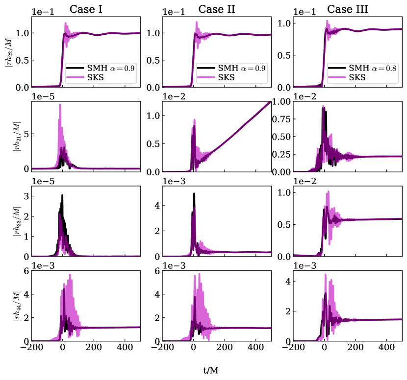
Figure 8: Mode amplitudes of waveforms for Case I, II and III with the highest resolution. Columns correspond to three cases, and rows are for different modes. For SMH initial data, we pick $\alpha=0.9$ for Case I and II, and $\alpha=0.8$ for Case III. Note that the linear growth of $h_{21}$ for Case II appears because only the initial part of the waveform is shown. Over the entire evolution, the mode is oscillatory. In general, the junk radiation of SMH initial data leaves the system faster. It is also smaller than the junk radiation of SKS for most of the modes. However, there are some modes, such as $h_{33}$, that have the same peak as SKS.

IV.2 Junk radiation and changes in parameters

Since the BHs in the initial data are not in true quasi-equilibrium, the masses and spins of BHs relax once the evolution begins, resulting in slight deviations from their initial values. In Figure 7, we show the change of irreducible mass $\Delta M_{\text{irr}}(t)=|M_{\text{irr}}(t)-M_{\text{irr}}(t=0)|$ and the change of spin $\Delta\chi(t)=|\chi(t)-\chi(t=0)|$ as functions of time, for three resolutions. We can see the variations are on the same order for both SMH and SKS initial data, but SMH has smaller oscillations. With the highest resolution, the deviation of SMH is smaller by a factor of $\sim 1.5-2$.

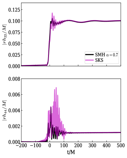
Figure 9: The $h_{22}$ and $h_{44}$ modes for the highest resolution of Case IV, an equal-mass BBH system with larger spins. The spins for both BHs are $(0,0,0.9)$, which we have not been able to run with SH initial data. We can still see that the junk radiation for SMH is less than SKS.

To study the junk radiation in the waveform, in Fig. 8 we plot the amplitudes of different spin weighted spherical harmonic modes $h_{lm}$, for Case I, II and III listed in Table 1 (Case IV will be discussed later). Note that the linear growth of $h_{21}$ for Case II appears because only the initial part of the waveform is shown; over the entire evolution, the mode is oscillatory.

We can see that the junk radiation of evolutions of SMH initial data is less than for SKS for most of the modes. In general, the junk radiation leaves the system faster for SMH initial data than for SKS. However, the decrease of junk radiation for SMH is not as significant as SH for low-spin BHs Varma et al. (2018). Some modes of SMH initial data, such as $h_{33}$, are similar to SKS. Comparing Cases II and III, we note that the junk radiation of $\alpha=0.8$ SMH is larger than that of $\alpha=0.9$ , presumably because $\alpha=0.8$ deviates more from SH initial data ($\alpha=1$). Note that Case II has similar junk radiation as Case III when both cases are evolved from SKS initial data; this suggests that the difference in junk radiation between Cases II and III seen in Figure 8 is probably not due to differences in parameters like the mass ratio.

For Case IV, a BBH system with dimensionless spins 0.9, we need to decrease $\alpha$ to 0.7, since for that large of spin $\alpha=0.8$ requires too high resolution and sometimes the initial data solver doesn’t converge. To speed up the evolution, we start the SMH initial data with fewer spherical shells around each BH than the standard choice made by SpEC. The comparison of the waveform is in Fig. 9, where we show only $h_{22}$ and $h_{44}$. We can see the junk radiation for SMH initial data is still less than for SKS. But the improvement is not as good as other cases. For modes other than $h_{22}$ and $h_{44}$ , we do not see improvements. The main reason appears to be that $\alpha=0.7$ deviates too much from $\alpha=1$, so that the benefit of SH initial data is reduced. In addition, in Fig. 10 we compare the accumulated CPU hours for evolutions of both initial data sets. We can see the initial computational efficiency for SMH initial data is much lower, but it gradually catches up after several shells are dropped. For evolutions of only a few orbits, the expense of evolving SMH initial data may not be worth the extra computational cost. But for evolutions of many orbits, the extra cost at the beginning of the evolution will be comparatively small.

In most of the evolutions shown here, shortly after the beginning of the simulation several spherical shells around each BH are dropped, leading to a smaller number of grid points, a larger time step, and overall greater computational efficiency. However, for a general evolution, we are not always ‘lucky’ enough to gain this efficiency, since the current algorithm for dropping spherical shells aims only to avoid narrow shells rather than to speed up the simulation. To improve the computational efficiency for all simulations, we could start with fewer spherical shells at $t=0$. However, the benefit of this change is limited without changing the shell-dropping algorithm. One workaround is to use smaller $\alpha$, which speeds up the simulation, but if $\alpha$ deviates too much from $\alpha=1$, we cannot have less junk radiation. Therefore, we suggest that the algorithm that divides the domain in to subdomains should be modified to account for computational efficiency during the evolution, or a better algorithm should be developed to initialize subdomains. Given such future algorithmic improvements, we could potentially run high-spin BBH evolution with larger $\alpha$, which can lead to less junk radiation.

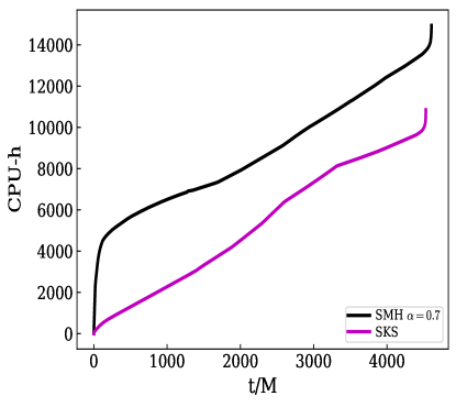
Figure 10: The accumulated CPU hours for evolutions of SMH and SKS initial data as functions of time. The BBH system is Case IV, and we plot results for the highest resolution. The initial computational efficiency of SMH initial data is much lower than for SKS, but after a short time both evolutions proceed at the same number of CPU hours per simulation time.

V Conclusion

In this paper, we extended SH initial data Varma et al. (2018) to higher-spin BBHs by introducing a class of spatial coordinate systems that represent a time-independent slicing of a single Kerr black hole and are characterized by a continuous parameter $\alpha$. This coordinate representation of Kerr is used to supply free data for the initial-value problem for BBH systems; we call the resulting initial-value solution SMH initial data. The harmonic $(\alpha=1)$ and KS $(\alpha=0)$ coordinate representations of Kerr are only two special cases of our new representation. The coordinate shape of the horizon becomes less spherical and more distorted for larger $\alpha$. Therefore for high-spin BHs, we pick $\alpha<1$ to decrease the distortion and ease requirements on very high resolution during the BBH simulation. At the same time, $\alpha$ should be close to 1 so that SMH initial data still has the desirable properties of SH initial data as shown in Ref. Varma et al. (2018), such as less junk radiation. We have tested that for SMH initial data with $\alpha=0$, i.e, harmonic time slicing with KS spatial coordinates, there is more junk radiation than for SKS initial data.

We have evolved four BBH systems with dimensionless spins 0.8 or 0.9 starting from SMH initial data with $\alpha$ between 0.7 and 0.9, and we compared with evolutions of the same system starting from SKS initial data. The first three cases, all with dimensionless spins 0.8, represent different situations: a non-precessing system with equal masses, a precessing system with random spin directions, and a non-precessing system with unequal masses. In general, the junk radiation of SMH initial data leaves the system faster than that of SKS. For most gravitational wave modes, the SMH initial data leads to less junk radiation. The exceptions, like the $h_{33}$ mode and the $h_{21}$ mode for Case III, have bursts with amplitudes similar to SKS. Furthermore, $\alpha=0.8$ SMH has more junk radiation than $\alpha=0.9$.

Using Case I as an example, we also studied other properties of the evolution, including constraint violations, computational efficiency, and changes in parameters. We found the values of the volume-weighted constraints for SMH initial data are smaller than those of SKS by factors of 10. Furthermore, the volume-weighted constraints of SMH initial data converge with resolution during the junk stage. However, $L^{2}$-norm constraints do not have such convergence. Therefore, the benefit is mainly from the outer regions, where there is less junk radiation.

At the beginning of the evolution for Case I, SMH requires more collocation points than SKS to reach the error tolerance because the horizon is distorted, hence it proceeds more slowly. At later times, SKS and SMH run at approximately the same rate, after both the computational efficiency on each time slice and the size of the time step increase for the SMH case.

For Case IV, which has BHs with dimensionless spin $0.9$, we found that we needed to decrease $\alpha$ to $0.7$. We simulated an equal-mass BBH system with equal dimensionless spins $\bm{\chi}_{1,2}=(0,0,0.9)$ and compared $h_{22}$ and $h_{44}$ for both SMH and SKS initial data sets. Junk radiation for SMH is still less than for SKS, but the improvement is not as good as the case of lower spin. The comparison of CPU hours for these two cases show that the initial computation efficiency for SMH initial data is much lower. But it gradually becomes the same as SKS after several shells are dropped.

We also found that the algorithm for choosing the number and sizes of subdomains in SpEC could use some improvement, particularly for the initial choice of subdomains and the early stages of the evolution. In most simulations but not all, AMR eventually chooses a subdomain distribution that increases computational efficiency. Some improvements can be gained by simply starting with fewer spherical shells around each BH, but we find that the effects of this change are limited. Therefore, the evolution of SMH initial data for high-spin BBH will benefit from either an algorithm to adjust subdomain sizes based on computational efficiency during the evolution, or a better algorithm to initialize subdomains. Those algorithmic improvements could allow us to run high-spin BBH evolutions with larger $\alpha$, which can give rise to less junk radiation.

Appendix A Details of MH coordinates

For a Kerr BH with an arbitrary spin vector $\bm{a}$, the transformations between KS spatial coordinates and MH spatial coordinates are given by

$$\bm{x}_{\text{KS}}= \frac{a^{2}+r(r-\alpha M)}{a^{2}+(r-\alpha M)^{2}}\bm{x}_{\text{MH}}$$

$$+ \frac{\alpha M}{a^{2}+(r-\alpha M)^{2}}(\bm{x}_{\text{MH}}\times\bm{a})$$

$$+ (\bm{x}_{\text{MH}}\cdot\bm{a})\bm{a}\frac{\alpha M}{(r-\alpha M)[a^{2}+(r-\alpha M)^{2}]},$$ (28)

where $a^{2}=\bm{a}\cdot\bm{a}$, and $r$ is the radial Boyer-Lindquist coordinate. For $\alpha=0$, we have $\bm{x}_{\text{KS}}=\bm{x}_{\text{MH}}$, i.e., the identity transformation. The Jacobian $C^{ij}_{\text{MH}}=\partial x_{\text{KS}}^{i}/\partial x_{\text{MH}}^{j}$ between KS and MH coordinates is given by

$$C^{ij}_{\text{MH}} =\frac{a^{2}+r(r-\alpha M)}{a^{2}+(r-\alpha M)^{2}}\delta^{ij}+\frac{\alpha M}{a^{2}+(r-\alpha M)^{2}}a_{k}\epsilon^{ijk}$$

$$+a^{i}a^{j}\frac{\alpha M}{(r-\alpha M)[a^{2}+(r-\alpha M)^{2}]}$$

$$+\frac{M\alpha[a^{2}-(r-M\alpha)^{2}]}{[a^{2}+(r-M\alpha)^{2}]^{2}}x_{\text{MH}}^{i}\partial^{j}r$$

$$-\frac{2M\alpha(r-M\alpha)}{(a^{2}+(r-M\alpha)^{2})^{2}}x^{\text{MH}}_{m}a_{k}\epsilon^{imk}\partial^{j}r$$

$$-x_{\text{MH}}^{m}a_{m}a^{i}\partial^{j}r\frac{M\alpha[a^{2}+3(r-M\alpha)^{2}]}{[a^{2}+(r-M\alpha)^{2}]^{2}(r-\alpha M)^{2}},$$ (29)

where $\epsilon^{ijk}$ is the Levi-Civita symbol, $\delta^{ij}$ is the Kronecker delta, and the Einstein summation convention is used. For $\alpha=1$, $C^{ij}_{\text{MH}}$ becomes $C^{ij}$ defined in Sec. III.4. By differentiating Eq. (22), we have

$$\partial_{i}r=\frac{x_{i}^{\text{MH}}+(\bm{a}\cdot\bm{x}^{\text{MH}})a_{i}/(r-\alpha M)^{2}}{2(r-\alpha M)\left[1-\frac{\bm{x}^{\text{MH}}\cdot\bm{x}^{\text{MH}}-a^{2}}{2(r-\alpha M)^{2}}\right]}.$$ (30)

With MH coordinates, the null covariant vector $l$ in Eq. (5) can be written as

$$l =\left(dt_{\text{MH}}+\frac{2M}{r-r_{-}}dr\right)$$

$$+\frac{(r-\alpha M)\bm{x}_{\text{MH}}-\bm{a}\times\bm{x}_{\text{MH}}+(\bm{a}\cdot\bm{x}_{\text{MH}})\bm{a}/(r-\alpha M)}{(r-\alpha M)^{2}+a^{2}}\cdot d\bm{x}_{\text{MH}},$$ (31)

where the first bracket corresponds to $dt_{\text{KS}}$ [see Eq. (12), with $t_{\text{MH}}=t_{\text{H}}$]. The scalar function $H$ in Eq. (5) is given by

$$H=\frac{Mr(r-\alpha M)^{2}}{r^{2}(r-\alpha M)^{2}+(\bm{a}\cdot\bm{x}_{\text{MH}})^{2}}.$$ (32)

In addition, the lapse function $N$ and the shift vector $N^{i}$ in MH coordinates are given by

$$N^{-2}=1+\frac{2M(r-\alpha M)^{2}}{r^{2}(r-\alpha M)^{2}+(\bm{a}\cdot\bm{x}_{\text{MH}})^{2}}\frac{r^{2}+(r+2M)r_{+}}{r-r_{-}},$$ (33)

$$N^{i}=N^{r}l^{i}+N^{\phi}\frac{a_{j}x^{\text{MH}}_{k}\epsilon^{jki}}{a},$$ (34)

with

$$N^{r}=N^{2}\frac{2Mr_{+}}{\rho^{2}},\quad N^{\phi}=-N^{2}\frac{a}{\rho^{2}}\frac{2M}{r-r_{-}},$$ (35)

$$\rho^{2}=r^{2}+a^{2}\cos^{2}\theta=r^{2}+\frac{(\bm{a}\cdot\bm{x}_{\text{MH}})^{2}}{(r-\alpha M)^{2}},\quad l^{i}=l_{i},$$ (36)

where $\theta$ is the polar Boyer-Lindquist coordinate, and $l_{i}$ is the spatial component of the null covariant vector $l$.

References

- Abbott et al. (2016) B. P. Abbott et al. (LIGO Scientific, Virgo), Phys. Rev. Lett. 116, 061102 (2016), arXiv:1602.03837 [gr-qc] .
- Abbott et al. (2019) B. Abbott et al. (LIGO Scientific, Virgo), Phys. Rev. X 9, 031040 (2019), arXiv:1811.12907 [astro-ph.HE] .
- Abbott et al. (2020) R. Abbott et al. (LIGO Scientific, Virgo), Phys. Rev. Lett. 125, 101102 (2020), arXiv:2009.01075 [gr-qc] .
- 190 (a) https://gracedb.ligo.org/superevents/S190412m/view/ (a).
- 190 (b) https://gracedb.ligo.org/superevents/S190425z/view/ (b).
- 190 (c) https://gracedb.ligo.org/superevents/S190814bv/view/ (c).
- Abadie et al. (2010) J. Abadie et al. (LIGO Scientific, VIRGO), Class. Quant. Grav. 27, 173001 (2010), arXiv:1003.2480 [astro-ph.HE] .
- Varma et al. (2019a) V. Varma, S. E. Field, M. A. Scheel, J. Blackman, D. Gerosa, L. C. Stein, L. E. Kidder, and H. P. Pfeiffer, Phys. Rev. Research. 1, 033015 (2019a), arXiv:1905.09300 [gr-qc] .
- Varma et al. (2019b) V. Varma, S. E. Field, M. A. Scheel, J. Blackman, L. E. Kidder, and H. P. Pfeiffer, Phys. Rev. D 99, 064045 (2019b), arXiv:1812.07865 [gr-qc] .
- Ossokine et al. (2020) S. Ossokine et al., (2020), arXiv:2004.09442 [gr-qc] .
- Cotesta et al. (2018) R. Cotesta, A. Buonanno, A. Bohé, A. Taracchini, I. Hinder, and S. Ossokine, Phys. Rev. D 98, 084028 (2018), arXiv:1803.10701 [gr-qc] .
- Bohé et al. (2017) A. Bohé et al., Phys. Rev. D95, 044028 (2017), arXiv:1611.03703 [gr-qc] .
- Pratten et al. (2020a) G. Pratten et al., (2020a), arXiv:2004.06503 [gr-qc] .
- García-Quirós et al. (2020) C. García-Quirós, M. Colleoni, S. Husa, H. Estellés, G. Pratten, A. Ramos-Buades, M. Mateu-Lucena, and R. Jaume, (2020), arXiv:2001.10914 [gr-qc] .
- Pratten et al. (2020b) G. Pratten, S. Husa, C. Garcia-Quiros, M. Colleoni, A. Ramos-Buades, H. Estelles, and R. Jaume, (2020b), arXiv:2001.11412 [gr-qc] .
- Alvi (2000) K. Alvi, Phys. Rev. D 61, 124013 (2000), arXiv:gr-qc/9912113 .
- Yunes and Tichy (2006) N. Yunes and W. Tichy, Phys. Rev. D 74, 064013 (2006), arXiv:gr-qc/0601046 .
- Johnson-McDaniel et al. (2009) N. K. Johnson-McDaniel, N. Yunes, W. Tichy, and B. J. Owen, Phys. Rev. D80, 124039 (2009), arXiv:0907.0891 [gr-qc] .
- Kelly et al. (2010) B. J. Kelly, W. Tichy, Y. Zlochower, M. Campanelli, and B. F. Whiting, Numerical relativity and data analysis. Proceedings, 3rd Annual Meeting, NRDA 2009, Potsdam, Germany, July 6-9, 2009, Class. Quant. Grav. 27, 114005 (2010), arXiv:0912.5311 [gr-qc] .
- Reifenberger and Tichy (2012) G. Reifenberger and W. Tichy, Phys. Rev. D 86, 064003 (2012), arXiv:1205.5502 [gr-qc] .
- Tichy (2017) W. Tichy, Rept. Prog. Phys. 80, 026901 (2017), arXiv:1610.03805 [gr-qc] .
- Lovelace (2009) G. Lovelace, Numerical relativity data analysis. Proceedings, 2nd Meeting, NRDA 2008, Syracuse, USA, August 11-14, 2008, Class. Quant. Grav. 26, 114002 (2009), arXiv:0812.3132 [gr-qc] .
- Varma et al. (2018) V. Varma, M. A. Scheel, and H. P. Pfeiffer, Phys. Rev. D98, 104011 (2018), arXiv:1808.08228 [gr-qc] .
- (24) https://www.black-holes.org/.
- York (1999) J. W. York, Jr., Phys. Rev. Lett. 82, 1350 (1999), arXiv:gr-qc/9810051 [gr-qc] .
- Pfeiffer and York (2003) H. P. Pfeiffer and J. W. York, Jr., Phys. Rev. D67, 044022 (2003), arXiv:gr-qc/0207095 [gr-qc] .
- Cook and Scheel (1997) G. B. Cook and M. A. Scheel, Phys. Rev. D 56, 4775 (1997).
- Boyle et al. (2019) M. Boyle et al., Class. Quant. Grav. 36, 195006 (2019), arXiv:1904.04831 [gr-qc] .
- Lovelace et al. (2008) G. Lovelace, R. Owen, H. P. Pfeiffer, and T. Chu, Phys. Rev. D78, 084017 (2008), arXiv:0805.4192 [gr-qc] .
- Szilagyi et al. (2009) B. Szilagyi, L. Lindblom, and M. A. Scheel, Phys. Rev. D80, 124010 (2009), arXiv:0909.3557 [gr-qc] .
- Kerr (1963) R. P. Kerr, Phys. Rev. Lett. 11, 237 (1963).
- Scheel et al. (2015) M. A. Scheel, M. Giesler, D. A. Hemberger, G. Lovelace, K. Kuper, M. Boyle, B. Szilágyi, and L. E. Kidder, Class. Quant. Grav. 32, 105009 (2015), arXiv:1412.1803 [gr-qc] .
- Boyd (2001) J. P. Boyd, Chebyshev and Fourier spectral methods (Courier Corporation, 2001).
- Szilágyi (2014) B. Szilágyi, Int. J. Mod. Phys. D23, 1430014 (2014), arXiv:1405.3693 [gr-qc] .
- Buonanno et al. (2011) A. Buonanno, L. E. Kidder, A. H. Mroue, H. P. Pfeiffer, and A. Taracchini, Phys. Rev. D83, 104034 (2011), arXiv:1012.1549 [gr-qc] .
- Lindblom et al. (2006) L. Lindblom, M. A. Scheel, L. E. Kidder, R. Owen, and O. Rinne, Class. Quant. Grav. 23, S447 (2006), arXiv:gr-qc/0512093 [gr-qc] .
- Ossokine et al. (2015) S. Ossokine, F. Foucart, H. P. Pfeiffer, M. Boyle, and B. Szilágyi, Class. Quant. Grav. 32, 245010 (2015), arXiv:1506.01689 [gr-qc] .
- Scheel et al. (2006) M. A. Scheel, H. P. Pfeiffer, L. Lindblom, L. E. Kidder, O. Rinne, and S. A. Teukolsky, Phys. Rev. D 74, 104006 (2006), arXiv:gr-qc/0607056 .