Exciton Dynamics in Conjugated Polymers

Abstract

Exciton dynamics in $\pi$-conjugated polymers encompass multiple time and length scales. Ultrafast femtosecond processes are intrachain and involve a quantum mechanical correlation of the exciton and nuclear degrees of freedom. In contrast, post-picosecond processes involve the incoherent Förster transfer of excitons between polymer chains. Exciton dynamics is also strongly determined by the spatial and temporal disorder that is ubiquitous in conjugated polymers. Since excitons are delocalized over hundreds of atoms, a theoretical understanding of these processes is only realistically possible by employing suitably parametrized coarse-grained exciton-phonon models. Moreover, to correctly account for ultrafast processes, the exciton and phonon modes must be treated on the same quantum mechanical basis and the Ehrenfest approximation must be abandoned. This further implies that sophisticated numerical techniques must be employed to solve these models. This review describes our current theoretical understanding of exciton dynamics in conjugated polymer systems. We begin by describing the energetic and spatial distribution of excitons in disordered polymer systems, and define the crucial concept of a ‘chromophore’ in conjugated polymers. We also discuss the role of exciton-nuclear coupling, emphasizing the distinction between ‘fast’ and ‘slow’ nuclear degrees of freedom in determining ‘self-trapping’ and ‘self-localization’ of exciton-polarons. Next, we discuss ultrafast intrachain exciton decoherence caused by exciton-phonon entanglement, which leads to fluorescence depolarization on the timescale of 10-fs. Interactions of the polymer with its environment causes the stochastic relaxation and localization of high-energy delocalized excitons onto chromophores. The coupling of excitons with torsional modes also leads to various dynamical processes. On sub-ps timescales it causes exciton-polaron formation (i.e., exciton localization and local polymer planarization), while on post-ps timescales stochastic torsional fluctuations cause exciton-polaron diffusion along the polymer chain. Finally, we describe a first-principles, Förster-type model of intrachain exciton transfer and diffusion, whose starting point is a realistic description of the donor and acceptor chromophores. We survey experimental results and explain how they can be understood in terms of our theoretical description of exciton dynamics coupled to information on polymer multiscale structures. The review also contains a brief critique of computational methods to simulate exciton dynamics.

I Introduction

The theoretical study of exciton dynamics in conjugated polymer systems is both a fascinating and complicated subject. One reason for this is that characterizing excitonic states themselves is a challenging task: conjugated polymers exhibit strong electron-electron interactions and electron-nuclear coupling, and are subject to spatial and temporal disorder. Another reason is that exciton dynamics is characterised by multiple (and often overlapping) time scales; it is determined by both intrinsic processes (e.g., coupling to nuclear degrees of freedom and electrostatic interactions) and extrinsic processes (e.g., polymer-solvent interactions); and it is both an intrachain and interchain process. Consequently, to make progress in both characterizing exciton states and correctly describing their dynamics, simplified, but realistic models are needed. Moreover, as even these simplified models describe many quantized degrees of freedom, sophisticated numerical techniques are required to solve them. Luckily, fundamental theoretical progress in developing numerical techniques means that simplified one-dimensional models of conjugated polymers are now soluble to a high degree of accuracy.

In addition to the application of various theoretical techniques to understand exciton dynamics, a wide range of time-resolved spectroscopic techniques have also been deployed. These include fluorescence depolarizationGrage et al. (2003); Ruseckas et al. (2005); Wells et al. (2007); Dykstra et al. (2009), three-pulse photon-echoDykstra et al. (2005); Yang, Dykstra, and Scholes (2005); Wells and Blank (2008); Sperling et al. (2008) and coherent electronic two-dimensional spectroscopyConsani et al. (2015). Some of the timescales extracted from these experiments are listed in Table 1; the purpose of this review is to describe their associated physical processes.

Polymer	State	Timescales	Citation
MEH-PPV	Solution	$\tau_{1}=50$ fs, $\tau_{2}=1-2$ ps	RefRuseckas et al. (2005)
MEH-PPV	Solution	$\tau_{1}=5-10$ fs, $\tau_{2}=100-200$ fs	RefCollini and Scholes (2009)
PDOPT	Film	$\tau=0.5-4$ ps	RefWestenhoff et al. (2006)
PDOPT	Solution	$\tau_{1}<1$ ps, $\tau_{2}=15-23$ ps	RefWestenhoff et al. (2006)
P3HT	Film	$\tau_{1}=300$ fs, $\tau_{2}=2.5$ ps, $\tau_{3}=40$ ps	RefWestenhoff et al. (2006)
P3HT	Solution	$\tau_{1}=700$ fs, $\tau_{2}=6$ ps, $\tau_{3}=41$ ps, $\tau_{4}=530$ ps	RefBanerji et al. (2011)
P3HT	Solution	$\tau_{1}=60-200$ fs, $\tau_{2}=1-2$ ps, $\tau_{3}=14-20$ ps	RefBusby et al. (2011)
P3HT	Solution	$\tau_{1}\lesssim 100$ fs, $\tau_{2}\sim 1-10$ ps	RefWells et al. (2007)

Table 1: Some of the dynamical timescales observed in conjugated polymers whose associated physical processes are summarized in Table 2.

As well as being of intrinsic interest, the experimental and theoretical activities to understand exciton dynamics in conjugated polymer systems are also motivated by the importance of this process in determining the efficiency of polymer electronic devices. In photovoltaic devices, large exciton diffusion lengths are necessary so that excitons can migrate efficiently to regions where charge separation can occur. However, precisely the opposite is required in light emitting devices, since diffusion leads to non-radiative quenching of the exciton.

Perhaps one of the reasons for the failure to fully exploit polymer electronic devices has been the difficulty in establishing the structure-function relationships which allow the development of rational design strategies. An understanding of the principles of exciton dynamics, relating this to multiscale polymer structures, and interpreting the associated spectroscopic signatures are all key ingredients to developing structure-function relationships. An earlier review explored the connection between structure and spectroscopyBarford and Marcus (2017). In this review we describe our current understanding of the important dynamical processes in conjugated polymers, beginning with photoexcitation and intrachain relaxation on ultrafast timescales ($\sim 10$ fs) to sub-ns interchain exciton transfer and diffusion. These key processes are summarized in Table 2.

Process	Consequences	Timescale	Section
Exciton-polaron self-trapping via coupling to fast C-C bond vibrations.	Exciton-site decoherence; ultrafast fluorescence depolarization.	$\sim 10$ fs	III.1
Energy relaxation from high-energy quasi-extended exciton states (QEESs) to low-energy local exciton ground states (LEGSs) via coupling to the environment.	Stochastic exciton density localization onto chromophores.	$\sim 100-200$ fs	III.2
Exciton-polaron self-localization via coupling to slow bond rotations in the under-damped regime.	Exciton density localization on a chromophore; ultrafast fluorescence depolarization.	$\sim 200-600$ fs	III.3
Exciton-polaron self-localization via coupling to slow bond rotations in the over-damped regime.	Exciton density localization on a chromophore; post-ps fluorescence depolarization.	$\sim 1-10$ ps	III.3
Stochastic torsional fluctuations inducing exciton ‘crawling’ and ‘skipping’ motion.	Intrachain exciton diffusion and energy fluctuations.	$\sim 3-30$ ps	IV
Interchromophore Förster resonant energy transfer.	Interchromophore exciton diffusion; post-ps spectral diffusion and fluorescence depolarization.	$\sim 10-100$ ps	V
Radiative decay.		$\sim 500$ ps

Table 2: The life and times of an exciton: Some of the key exciton dynamical processes, encompassing over four-orders of magnitude, that occur in conjugated polymer systems.

The plan of this review is the following. We begin by briefly describing some theoretical techniques for simulating exciton dynamics and emphasize the failures of simple methods. As already mentioned, excitons themselves are fascinating quasiparticles, so before describing their dynamics, in Section III we start by describing their stationary states. We stress the role of low-dimensionality, disorder and electron-phonon coupling, and we discuss the fundamental concept of a chromophore. Next, in Section IV, we describe the sub-ps processes of intrachain exciton decoherence, relaxation and localization, which - starting from an arbitrary photoexcited state - results in an exciton forming a chromophore. We next turn to describe the exciton (and energy) transfer processes occurring on post-ps timescales. First, in Section V, we describe the primarily adiabatic intrachain motion of excitons caused by stochastic torsional fluctuations, and second, in Section VI, we describe nonadiabatic interchain exciton transfer. We conclude and address outstanding questions in Section VII.

II A Brief Critique of Theoretical Techniques

A theoretical description of exciton dynamics in conjugated polymers poses considerable challenges, as it requires a rigorous treatment of electronic excited states and their coupling to the nuclear degrees of freedom. Furthermore, conjugated polymers consist of thousands of atoms and tens of thousands of electrons. Thus, as the Hilbert space grows exponentially with the number of degrees of freedom, approximate treatments of excitonic dynamics are therefore inevitable. There are two broad approaches to a theoretical treatment. One approach is to construct ab initio Hamiltonians, with an exact as possible representation of the degrees of freedom, and then to solve these Hamiltonians with various degrees of accuracy. Another approach (albeit less common in theoretical chemistry) is to construct effective Hamiltonians with fewer degrees of freedom, such as the Frenkel-Holstein model described in Section IV. These effective Hamiltonians might be parameterized via a direct mapping from ab initio Hamiltonians (e.g., see Appendix H in refBarford (2013a), Appendix A in refBarford and Marcus (2014) and various papers by Burghardt and coworkersBinder et al. (2014, )) or else semiempiricallyMarcus, Tozer, and Barford (2014). A significant advantage of effective Hamiltonians over their ab initio counterparts is that they can be solved for larger systems over longer timescales and to a higher level of accuracy.

As the Ehrenfest method is a widely used approximation to study charge and exciton dynamics in conjugated polymers, we briefly explain this method and describe the important ways in which it fails. (For a fuller treatment, seeHorsfield et al. (2006); Nelson et al. (2020).) The Ehrenfest method makes two key approximations. The first approximation is to treat the nuclei classically. This means that nuclear quantum tunneling and zero-point energies are neglected, and that exciton-polarons are not correctly described (see Section III.3). The second assumption is that the total wavefunction is a product of the electronic and nuclear wavefunctions. This means that there is no entanglement between the electrons and nuclei, and so the nuclei cannot cause decoherence of the electronic degrees of freedom (see Section IV.1). A simple product wavefunction also implies that the nuclei move in a mean field potential determined by the electrons. This means that a splitting of the nuclear wave packet when passing through a conical intersection or an avoided crossing does not occur (see Section IV.2), and that there is an incorrect description of energy transfer between the electronic and nuclear degrees of freedom (see Section V.4). As will be discussed in the course of this review, these failures mean that in general the Ehrenfest method is not a reliable one to treat ultrafast excitonic dynamics in conjugated polymers.

Various theoretical techniques have been proposed to rectify the failures of the Ehrenfest method; for example, the surface-hopping techniqueTully (1990, 2012), while still keeping the nuclei classical, partially rectifies the failures at conical interactions. More sophisticated approaches, for example the MC-TDHF and TEBD methods, quantize the nuclear degrees of freedom and do not assume a product wavefunction.

For a given electronic potential energy surface (PES), the multiconfigurational-time dependent Hartree-Fock (MC-TDHF) methodBeck et al. (2000) is an (in principle) exact treatment of nuclear wavepacket propagation, although in practice exponential scaling of the Hilbert space means that a truncation is required. In addition, this method is only as reliable as the representation of the PES.

In the time-evolving block decimation (TEBD) methodVidal (2003, 2004) a quantum state, $|\Psi\rangle$, is represented by a matrix product state (MPS)Schöllwock (2011). Its time evolution is determined via

$$|\Psi(t+\delta t\rangle=\exp(-\textrm{i}\hat{H}\delta t/\hbar)|\Psi(t)\rangle,$$ (1)

where $\hat{H}$ is the system Hamiltonian and the action of the evolution operator is performed via a Trotter decomposition. Since the action of the evolution operator expands the Hilbert space, $|\Psi\rangle$ is subsequently compressed via a singular value decomposition (SVD). Importantly, this approach is ‘numerically exact’ as long as the truncation parameter exceeds $2^{S}$, where $S$ is the entanglement entropy, defined by $S=-\sum_{\alpha}\omega_{\alpha}\textrm{ln}_{2}\omega_{\alpha}$ and $\{\omega\}$ are the singular values obtained at the SVD. The TEBD method permits the electronic and nuclear degrees of freedom to be treated as quantum variables on an equal footing. It thus rectifies all of the failures of the Ehrenfest method described above and, unlike the MC-TDHF method, it is not limited by the representation of the PES. It can, however, only be applied to quantum systems described by one-dimensional lattice HamiltoniansMannouch, Barford, and Al-Assam (2018). Luckily, as described in Section IV, such model Hamiltonians are readily constructed to describe exciton dynamics in conjugated polymers.

III Excitons in Conjugated Polymers

Before discussing the dynamics of excitons, we begin by describing exciton stationary states in static conjugated polymers.

III.1 Two-particle model

An exciton is a Coulombically bound electron-hole pair formed by the linear combination of electron-hole excitations (for further details seeBarford (2013a); Kobayashi (1993); Barford (2013b)). In a one-dimensional conjugated polymer an exciton is described by the two-particle wavefunction, $\Phi_{mj}(r,R)=\psi_{m}(r)\Psi_{j}(R)$.

$\Psi_{j}(R)$ is the center-of-mass wavefunction, which will be discussed shortly. Before doing that, we first discuss the relative wavefunction, $\psi_{m}(r)$, which describes a particle bound to a screened Coulomb potential, where $r$ is the electron-hole separation and $m$ is the principal quantum number. The electron and hole of an exciton in a one-dimensional semiconducting polymer are more strongly bound than in a three-dimensional inorganic semiconductor for two key reasons.Barford (2013a, b) First, because of the low dielectric constant and relatively large electronic effective mass in $\pi$-conjugated systems the effective Rydberg is typically $50$ times larger than for inorganic systems. Second, dimensionality plays a role: in particular, the one-dimensional Schrödinger equation for the relative particleLoudon (2016); Barford, Bursill, and Smith (2002) predicts a strongly bound state split-off from the Rydberg series. This state is the $m=1$ Frenkel (‘$1B_{u}$’) exciton, with a binding energy of $\sim 1$ eV and an electron-hole wavefunction confined to a single monomer. The first exciton in the ‘Rydberg’ series is the $m=2$ charge-transfer (‘$2A_{g}$’) exciton.

With the exception of donor-acceptor copolymers, conjugated polymers are generally non-polar, which means that each $p$-orbital has an average occupancy of one electron. This implies an approximate electron-hole symmetry. Electron-hole symmetry has a number of consequences for the character and properties of excitons. First, it means that the relative wavefunction exhibits electron-hole parity, i.e., $\psi_{m}(r)=+\psi_{m}(-r)$ when $m$ is odd and $\psi_{m}(r)=-\psi_{m}(-r)$ when $m$ is even. Second, the transition density, $\langle\textrm{EX}|\hat{N}_{i}|\textrm{GS}\rangle$, vanishes for odd-parity (i.e., even $m$) excitons. This means that such excitons are not optically active, and importantly for dynamical processes, their Förster exciton transfer rate (defined in Section VI.1) vanishes.

Since Frenkel excitons are the primary photoexcited states of conjugated polymers, their dynamics is the subject of this review. Their delocalization along the polymer chain of $N$ monomers is described by the Frenkel Hamiltonian,

$$\hat{H}_{F} = \sum_{n=1}^{N}\epsilon_{n}\hat{N}_{n}+\sum_{n=1}^{N-1}J_{n}\hat{T}_{n,n+1},$$ (2)

where $n=(R/d)$ labels a monomer and $d$ is the intermonomer separation. The energy to excite a Frenkel exciton on monomer $n$ is $\epsilon_{n}$, where $\hat{N}_{n}=\ket{n}\bra{n}$ is the Frenkel exciton number operator.

In principle, excitons delocalize along the chain via two mechanismsBarford and Trembath (2009); Barford (2013b). First, for even-parity (odd $m$) singlet excitons there is a Coulomb-induced (or through space) mechanism. This is the familiar mechanism of Förster energy transfer. The exciton transfer integral for this process is

$$J_{DA}=\sum_{\begin{subarray}{c}i\in D\\ j\in A\end{subarray}}V_{ij}\left[{{}_{D}}\langle\textrm{GS}|\hat{N}_{i}|\textrm{EX}\rangle_{D}\right]\left[{{}_{A}}\langle\textrm{EX}|\hat{N}_{j}|\textrm{GS}\rangle_{A}\right].$$ (3)

The sum is over sites $i$ in the donor monomer and $j$ in the acceptor monomer, and $V_{ij}$ is the Coulomb interaction between these sites. In the point-dipole approximation Eq. (3) becomes

$$J_{DA}=\frac{\kappa_{mn}\mu_{0}^{2}}{4\pi\varepsilon_{r}\varepsilon_{0}R_{mn}^{3}},$$ (4)

where $\mu_{0}$ is the transition dipole moment of a single monomer and ${R}_{mn}$ is the distance between the monomers $m$ and $n$. $\kappa_{mn}$ is the orientational factor,

$$\kappa_{mn}=\bm{\hat{r}_{m}}\cdot\bm{\hat{r}_{n}}-3(\bm{\hat{R}_{mn}}\cdot\bm{\hat{r}_{m}})(\bm{\hat{R}_{mn}}\cdot\bm{\hat{r}_{n}}),$$ (5)

where $\bm{\hat{r}_{m}}$ is a unit vector parallel to the dipole on monomer $m$ and $\bm{\hat{R}_{mn}}$ is a unit vector parallel to the vector joining monomers $m$ and $n$. For colinear monomers, the nearest neighbor through space transfer integral is

$$J_{DA}=-\frac{2\mu_{0}^{2}}{4\pi\varepsilon_{r}\varepsilon_{0}d^{3}}.$$ (6)

Second, for all excitons there is a super-exchange (or through bond) mechanism, whose origin lies in a virtual fluctuation from a Frenkel exciton on a single monomer to a charge-transfer exciton spanning two monomers back to a Frenkel exciton on a neighboring monomer. The energy scale for this process, obtained from second order perturbation theoryBarford (2013a), is

$$J_{SE}(\theta)\propto-\frac{t(\theta)^{2}}{\Delta E},$$ (7)

where $t(\theta)$ (defined in Eq. (12)) is proportional to the overlap of $p$-orbitals neighboring a bridging bond, i.e., $t(\phi)\propto\cos\theta$ and $\theta$ is the torsional (or dihedral) angle between neighboring monomers. $\Delta E$ is the difference in energy between a charge-transfer and Frenkel exciton.

The total exciton transfer integral is thus

$$J_{n}=J_{\text{DA}}+J_{\text{SE}}^{0}\cos^{2}{\theta_{n}}.$$ (8)

The bond-order operator,

$$\hat{T}_{n,n+1}=\left(\ket{n}\bra{n+1}+\ket{n+1}\bra{n}\right),$$ (9)

represents the hopping of the Frenkel exciton between monomers $n$ and $n+1$. Evidently, $J_{SE}$ vanishes when $\theta=0$, but $J_{DA}$ will not. Therefore, even if $J_{SE}$ vanishes because of negligible $p$-orbital overlap between neighboring monomers, singlet even-parity excitons can still retain phase coherence over the ‘conjugation break’Barford et al. (2010). This observation has important implications for the definition of chromophores, as discussed in Section III.2.

Eq. (2) represents a ‘coarse-graining’ of the exciton degrees of freedom. The key assumption is that we can replace the atomist detail of each monomer (or moiety) and replace it by a ‘coarse-grained’ site, as illustrated in Fig. 1. All that remains is to describe how the Frenkel exciton delocalises along the chain, which is controlled by the two sets of parameters, $\{\epsilon\}$ and $\{J\}$. Since $J$ is negative, a conjugated polymer is equivalent to a molecular J-aggregate.

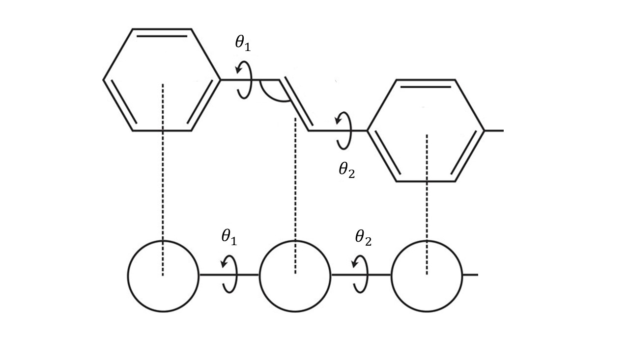
Figure 1: The mapping of a polymer chain conformation to a coarse-grained linear site model. Each site corresponds to a moiety along the polymer chain, with the connection between sites characterised by the torsional (or dihedral) angle, $\theta$.

The eigenfunctions of $\hat{H}_{F}$ are the center-of-mass wavefunctions, $\Psi_{j}(n)$, where $j$ is the associated quantum number. For a linear, uniform polymer (i.e., $\epsilon_{n}\equiv\epsilon_{0}$ and $J_{n}\equiv J_{0}$)

$$\Psi_{j}(n)=\left(\frac{2}{N+1}\right)^{1/2}\sum_{n=1}^{N}\sin\left(\frac{\pi jn}{N+1}\right),$$ (10)

forming a band of states with energy

$$E_{j}=\epsilon_{0}+2J_{0}\cos\left(\frac{\pi j}{N+1}\right).$$ (11)

The family of excitons with different $j$ values corresponds to the Frenkel exciton band with different center-of-mass momenta. In emissive polymers the $j=1$ Frenkel exciton is generally labeled the $1^{1}B_{u}$ state.

III.2 Role of static disorder: local exciton ground states and quasiextended exciton states

Polymers are rarely free from some kind of disorder and thus the form of Eq. (10) is not valid for the center-of-mass wavefunction in realistic systems. Polymers in solution are necessarily conformationally disordered as a consequence of thermal fluctuations (as described in Section V). Polymers in the condensed phase usually exhibit glassy, disordered conformations as consequence of being quenched from solution. Conformational disorder implies that the dihedral angles, $\{\theta\}$ are disordered, which by virtue of Eq. (8) implies that the exciton transfer integrals are also disordered.

As well as conformational disorder, polymers are also subject to chemical and environmental disorder (arising, for example, from density fluctuations). This type of disorder affects the energy to excite a Frenkel exciton on a monomer (or coarse-grained site).

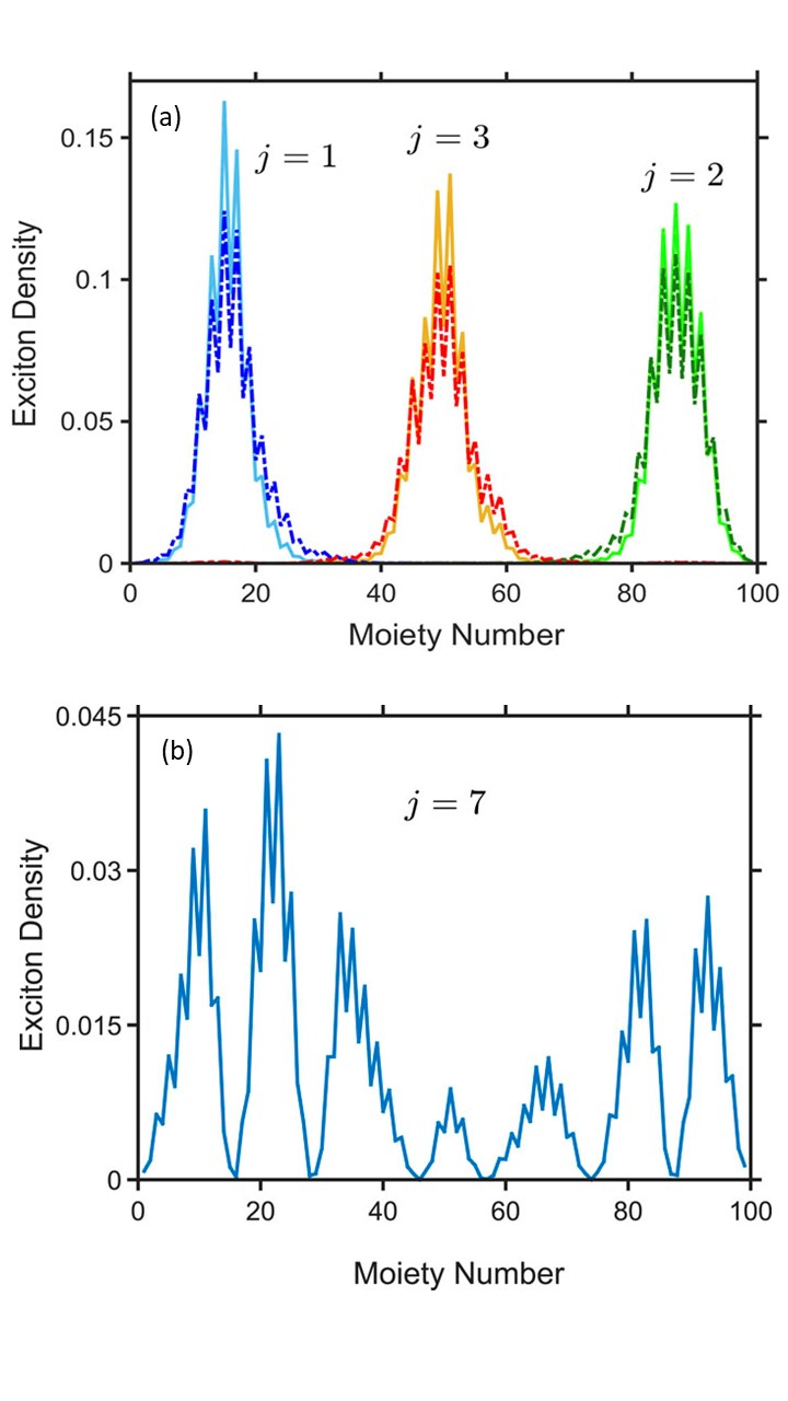
Figure 2: (a) The density of three local exciton ground states (LEGSs, dotted curves) and the three vibrationally relaxed states (VRSs, solid curves) for one particular static conformation of a PPV polymer chain made up of 50 monomers. The exciton center-of-mass quantum number, $j$, for each state is also shown. (b) The exciton density of a quasiextended exciton state (QEES), with quantum number $j=7$. Reproduced from J. Chem. Phys. 148, 034901 (2018) with the permission of AIP publishing.

As first realized by AndersonAnderson (1958), disorder localizes a quantum particle (in our case, the exciton center-of-mass particle), and determines their energetic and spatial distributions. The origin of this localization is the wave-like nature of a quantum particle and the constructive and destructive interference it experiences as it scatters off a random potential. Malyshev and MalyshevMalyshev and Malyshev (2001a, b) further observed that in one-dimensional systems there are a class of states in the low energy tail of the density of states that are superlocalized, named local exciton ground states (LEGSsMalyshev and Malyshev (2001a, b); Makhov and Barford (2010)). LEGSs are essentially nodeless, non-overlapping wavefunctions that together spatially span the entire chain. They are local ground states, because for the individual parts of the chain that they span there are no lower energy states. A consequence of the essentially nodeless quality of LEGSs is that the square of their transition dipole moment scales as their sizeMakhov and Barford (2010). Thus, LEGSs define chromophores (or spectroscopic segments), namely the irreducible parts of a polymer chain that absorb and emit light. Fig. 2(a) illustrates the three LEGSs for a particular conformation of PPV with 50 monomers.

Some researchers claim that ‘conjugation-breaks’ (or more correctly, minimum thresholds in the $p_{z}$-orbital overlap) define the boundaries of chromophoresAthanasopoulos et al. (2008). In contrast, we suggest that it is the disorder that determines the average chromophore size, but ‘conjugation-breaks’ can ‘pin’ the chromophore boundaries. Thus, if the average distance between conjugation breaks is smaller than the chromophore size, chromophores will span conjugation breaks but they may also be separated by them. Conversely, if average distance between conjugation breaks is larger than the chromophore size the chromophore boundaries are largely unaffected by the breaks. The former scenario occurs in polymers with shallow torsional potentials, e.g., polythiopheneBarford et al. (2010).

Higher energy lying states are also localized, but are nodeful and generally spatially overlap a number of low-lying LEGSs. These states are named quasiextended exciton states (QEESs) and an example is illustrated in Fig. 2(b).

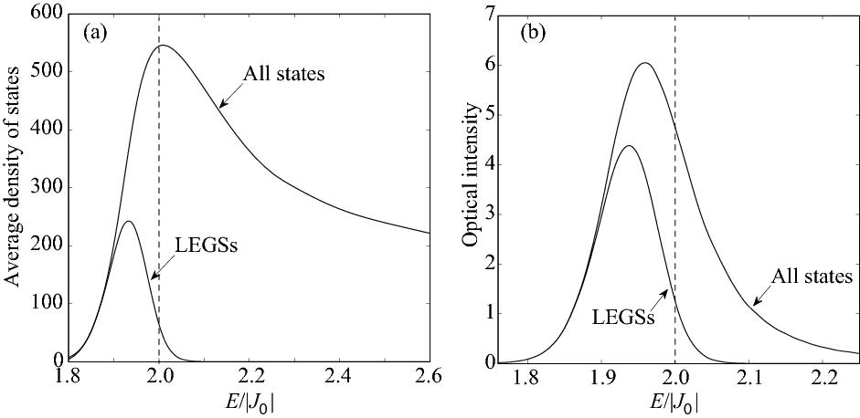
Figure 3: (a) The energy density of states and (b) the optical absorption (neglecting the vibronic progression) of the manifold of Frenkel excitons (where $|\sigma_{J}/J_{0}|=0.1$). The width of the LEGSs density of states $\sim|J_{0}||\sigma_{J}/J_{0}|^{4/3}$. Similarly, the width of the optical absorption from both the LEGSs and all states $\sim|J_{0}||\sigma_{J}/J_{0}|^{4/3}$. The band edge for an ordered chain is at $2|J_{0}|$ (indicated by the dashed lines), so LEGSs generally lie in the Lifshitz (or Urbach) tail of the density of states, i.e., $E<2|J_{0}|$.

When the disorder is Gaussian distributed with a standard deviation $\sigma$, single parameter scaling theoryKramer and Mackinnon (1993) provides some exact results about the spatial and energetic distribution of the exciton center-of-mass states:

1. The localization length $L_{loc}\sim({|J_{0}|}/{\sigma})^{2/3}$ at the band edge and as $L_{loc}\sim({|J_{0}|}/{\sigma})^{4/3}$ at the band center.

2. As a consequence of exchange narrowing, the width of the density of states occupied by LEGSs scales as $\sigma/\sqrt{L_{loc}}\sim\sigma^{4/3}$. Similarly, the optical absorption is inhomogeneously narrowed with a line width $\sim\sigma^{4/3}$.

3. The fraction of LEGSs scales as $1/L_{loc}\sim\sigma^{2/3}$.

These points are illustrated in Fig. 3, which shows the Frenkel exciton density of states and optical absorption for a particular value of disorder. Evidently, although LEGSs are a small fraction of the total number of states, they dominate the optical absorption.

This section has described LEGSs (or chromophores) as static objects defined by static disorder. However, as discussed in Section V, dynamically torsional fluctuations also render the conformational disorder dynamic causing the LEGSs to evolve adiabatically. As a consequence, the chromophores ‘crawl’ along the polymer chain.

III.3 Role of electron-nuclear coupling: exciton-polarons

As well as disorder, another important process in determining exciton dynamics and spectroscopy is the coupling of an exciton to nuclear degrees of freedom; in a conjugated polymer these are fast C-C bond vibrations and slow monomer rotations. In this section we briefly review the origin of this coupling and then discuss exciton-polarons.

III.3.1 Origin of electron-nuclear coupling

When a nucleus moves, either by a linear displacement or by a rotation about a fixed point, there is a change in the electronic overlap between neighboring atomic orbitals. Assuming that neighboring $p$-orbitals lie in the same plane normal to the bond with a relative twist angle of $\theta$, the resonance integral between a pair of orbitals separated by $r$ isMulliken et al. (1949)

$$t(\theta)=t(r)\cos\theta=\beta\exp(-\alpha r)\cos\theta,$$ (12)

where $t(r)<0$. The kinetic energy contribution to the Hamiltonian is

$$\hat{H}_{\textrm{ke}}=t(r)\cos\theta\times{\hat{T}},$$ (13)

where the bond-order operator, ${\hat{T}}$, is defined in Eq. (9). Treating $r$ and $\theta$ as dynamical variables, suppose that the $\sigma$-electrons of a conjugated molecule and steric hinderances provide equilibrium values of $r=r_{0}$ and $\theta=\theta_{0}$, with corresponding elastic potentials of

$$V_{\textrm{vib}}=\frac{1}{2}K_{\textrm{vib}}^{\sigma}(r-r_{0})^{2}$$ (14)

and

$$V_{\textrm{rot}}=\frac{1}{2}K_{\textrm{rot}}^{\sigma}(\theta-\theta_{0})^{2}.$$ (15)

The coupling of the $\pi$-electrons to the nuclei changes these equilibrium values and the elastic constants.

To see this, we use the Hellmann-Feynman to determine the force on the bond. The linear displacement force is

$$f=-\frac{\partial E}{\partial r} =-\big{\langle}\frac{\partial\hat{H}_{\textrm{ke}}}{\partial r}\big{\rangle}$$ (16)

$$=\alpha t(r)\cos\theta\langle{\hat{T}}\rangle-K_{\textrm{vib}}^{\sigma}(r-r_{0}).$$

Thus, to first order in the change of bond length, $\delta r=(r-r_{0})$, the equilibrium distortion is

$$\delta r=\alpha t(r_{0})\cos\theta\langle{\hat{T}}\rangle/K_{\textrm{vib}}^{\sigma},$$ (17)

which is negative because it is favorable to shorten the bond to increase the electronic overlap.

Similarly, the torque around the bond is

$$\Gamma=-\frac{\partial E}{\partial\theta} =-\big{\langle}\frac{\partial\hat{H}_{ke}}{\partial\theta}\big{\rangle}$$ (18)

$$=t(r)\sin\theta\langle{\hat{T}}\rangle-K_{\textrm{rot}}^{\sigma}(\theta-\theta_{0})$$

and the equilibrium change of bond angle, $\delta\theta=(\theta-\theta_{0})$, is

$$\delta\theta=t(r)\sin\theta_{0}\langle{\hat{T}}\rangle/K_{\textrm{rot}}^{\sigma},$$ (19)

which is also negative, again because it is favorable to increase the electronic overlap. Thus, the $\pi$-electron couplings act to planarize the chain.

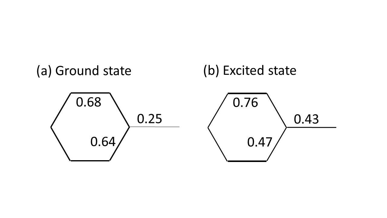
Figure 4: The $\pi$-bond order expectation values, $\langle\hat{T}\rangle$, for (a) the ground state and (b) the excited state, showing the benzenoid-quinoid transition. As Eq. (19) and Eq. (III.3.1) indicate, the larger bond order of the bridging bond in the excited state implies a smaller dihedral angle and a stiffer torsional potential than the ground state.

The electron-nuclear coupling also changes the elastic constants. Assuming a harmonic potential, the new rotational spring constant is

$$K_{\textrm{rot}}^{\pi}= \frac{\partial^{2}E}{\partial\theta^{2}}$$

$$= -t(r_{0})\cos\theta_{0}\langle{\hat{T}}\rangle+K_{\textrm{rot}}^{\sigma}$$ (20)

and thus $K_{\textrm{rot}}^{\pi}>K_{\textrm{rot}}^{\sigma}$ (because $t(r_{0})<0$).

Interestingly, as shown in Fig. 4, because $\langle{\hat{T}}\rangle_{EX}>\langle{\hat{T}}\rangle_{GS}$ for the bridging bond in phenyl-based systems, the torsional angle is smaller and the potential is stiffer in the excited state (as a result of the benzenoid to quinoid distortion)Beenken and Lischka (2005).

III.3.2 Exciton-polarons

An exciton that couples to a set of harmonic oscillators, e.g., bond vibrations or torsional oscillations, becomes ‘self-trapped’. Self-trapping means that the coupling between the exciton and oscillators causes a local displacement of the oscillator that is proportional to the local exciton densityRashba (1957a, b, c); Holstein (1959a, b) (as illustrated in the next section). Alternatively, it is said that the exciton is dressed by a cloud of oscillators. Such a quasiparticle is named an exciton-polaron. As there is no barrier to self-trapping in one-dimensional systemsRashba and Sturge (1982), there is always an associated relaxation energy.

If the exciton and oscillators are all treated quantum mechanically, then in a translationally invariant system the exciton-polaron forms a Bloch state and is not localized. However, if the oscillators are treated classically, the non-linear feedback induced by the exciton-oscillator coupling self-localizes the exciton-polaron and ‘spontaneously’ breaks the translational symmetry. This is a self-localized (or auto-localized) ‘Landau polaron’.Landau (1933); Campbell, Bishop, and Fesser (1982) Notice that self-trapping is a necessary but not sufficient condition for self-localization. Self-localization always occurs in the limit of vanishing oscillator frequency (i.e., the adiabatic or classical limit) and vanishing disorder.Tozer and Barford (2014)

Whether or not an exciton-polaron is self-localized in practice, however, depends on the strength of the disorder and the vibrational frequency of the oscillators. Qualitatively, an exciton coupling to fast oscillators (e.g., C-C bond vibrations) forms an exciton-polaron with an effective mass only slightly larger than a bare excitonTozer and Barford (2014). For realistic values of disorder, such an exciton-polaron is not self-localized. This is illustrated in Fig. 2(a), which shows the three lowest solutions of the Frenkel-Holstein model (described in Section IV.1), known as vibrationally relaxed states (VRSs). As we see, the density of the VRSs mirrors that of the Anderson-localized LEGSs. Conversely, an exciton coupling to slow oscillators (e.g., bridging-bond rotations) forms an exciton-polaron with a large effective mass. Such an exction-polaron is self-localized (as described in Section IV.3 and shown in Fig. 6).

IV Intrachain Decoherence, Relaxation and Localization

Having qualitatively described the stationary states of excitons in conjugated polymers, we now turn to a discussion of exciton dynamics.

IV.1 Role of fast C-C bond vibrations

After photoexcitation or charge combination after injection, the fastest process is the coupling of the exciton to C-C bond stretches. We now describe the resulting exciton-polaron formation and the loss of exciton-site coherence.

As we saw in Section III.3, bond distortions couple to electrons. Using Eq. (13), it can be shownMarcus, Tozer, and Barford (2014) that the coupling of local normal modes (e.g., vinyl-unit bond stretches or phenyl-ring symmetric breathing modes) to a Frenkel exciton is conveniently described by the Frenkel-Holstein modelHolstein (1959a); Marcus, Tozer, and Barford (2014),

$$\hat{H}_{FH} = \hat{H}_{F}-A\hbar\omega_{\textrm{vib}}\sum_{n=1}^{N}\tilde{Q}_{n}\hat{N}_{n}+\frac{\hbar\omega_{\textrm{vib}}}{2}\sum_{n=1}^{N}\left(\tilde{Q}_{n}^{2}+\tilde{P}_{n}^{2}\right).$$

$\hat{H}_{F}$ is the Frenkel Hamiltonian, defined in Eq. (2), while $\tilde{Q}=(K_{\textrm{vib}}/\hbar\omega_{\textrm{vib}})^{1/2}Q$ and $\tilde{P}=(\omega_{\textrm{vib}}/\hbar K_{\textrm{vib}})^{1/2}P$ are the dimensionless displacement and momentum of the normal mode. The second term on the right-hand-side of Eq. (IV.1) indicates that the normal mode couples linearly to the local exciton density. $A$ is the dimensionless exciton-phonon coupling constant, which introduces the important polaronic parameter, namely the local Huang-Rhys factor

$$S=\frac{A^{2}}{2}.$$ (22)

The final term is the sum of the elastic and kinetic energies of the harmonic oscillator, where $\omega_{\textrm{vib}}$ and $K_{\textrm{vib}}$ are the angular frequency and force constant of the oscillator, respectively. The Frenkel-Holstein model is another example of a coarse-grained Hamiltonian which, in addition to coarse-graining the exciton motion, assumes that the atomistic motion of the carbon nuclei can be replaced by appropriate local normal modes.

Exciton-nuclear dynamics is often modeled via the Ehrenfest approximation, which treats the nuclear coordinates as classical variables moving in a mean field determined by the exciton. However, as described in Section II, the Ehrenfest approximation fails to correctly describe ultrafast dynamical processes. A correct description of the coupled exciton-nuclear dynamics therefore requires a full quantum mechanical treatment of the system. This is achieved by introducing the harmonic oscillator raising and lowering operators, $\hat{b}_{n}^{\dagger}$ and $\hat{b}_{n}$, for the normal modes i.e., $\tilde{Q}_{n}\rightarrow\hat{\tilde{Q}}_{n}=(\hat{b}_{n}^{\dagger}+\hat{b}_{n})/\sqrt{2}$ and $\tilde{P}_{n}\rightarrow\hat{\tilde{P}}_{n}=i(\hat{b}_{n}^{\dagger}-\hat{b}_{n})\sqrt{2}$. The time evolution of the quantum system can then conveniently be simulated via the TEBD method, as briefly described in Section II.

Since the photoexcited system has a different electronic bond order than the ground state, an instantaneous force is established on the nuclei. As described in Section III.3, this force creates an exciton-polaron, whose spatial size is quantified by the exciton-phonon correlation functionHoffmann and Soos (2002)

$$C_{n}^{\textrm{ex-ph}}(t)\propto\sum_{m}\langle\hat{N}_{m}\hat{\tilde{Q}}_{m+n}\rangle.$$ (23)

$C_{n}^{\textrm{ex-ph}}$ correlates the local phonon displacement, $Q$, with the instantaneous exciton density, $N$, $n$ monomers away. $C_{n}^{\textrm{ex-ph}}(t)$, illustrated in Fig. 5, shows that the exciton-polaron is established within 10 fs (i.e., within half the period of a C-C bond vibration) of photoexcitation. The temporal oscillations, determined by the C-C bond vibrations, are damped as energy is dissipated into the vibrational degrees of freedom, which acts as a heat bath for the exciton. The exciton-phonon spatial correlations decay exponentially, extending over ca. 10 monomers. This short range correlation occurs because the C-C bond can respond relatively quickly to the exciton’s motion.

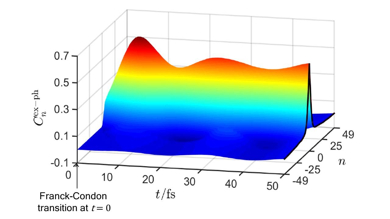
Figure 5: The time-dependence of the exciton-phonon correlation function, Eq. (23), after photoexcitation at time $t=0$. It fits the form $C_{n}^{\text{ex-ph}}=C_{0}\exp(-n/\xi)$ as $t\rightarrow\infty$, where $\xi\sim 10$. $n$ is a monomer index. The vibrational period is $20$ fs.

The ultrafast establishment of quantum mechanically correlated exciton-phonon motion causes an ultrafast decay of off-diagonal-long-range-order (ODLRO) in the exciton site-basis density matrix. This is quantified viaKuhn and Sundstrom (1997); Smyth, Fassioli, and Scholes (2012)

$$C_{n}^{\textrm{coh}}(t)=\sum_{m}\left|\rho_{m,m+n}\right|,$$ (24)

where $\rho_{m,m^{\prime}}$ is the exciton reduced density matrix obtained by tracing over the vibrational degrees of freedom. $C_{n}^{\textrm{coh}}(t)$ is displayed in Fig. 6, showing that ODLRO is lost within 10 fs. The loss of ODLRO is further quantified by the coherence number, defined by

$$N^{\textrm{coh}}=\sum_{n}C_{n}^{\textrm{coh}},$$ (25)

and shown in the inset of Fig. 6. Again, $N^{\textrm{coh}}$ decays to ca. 10 monomers in ca. 10 fs, reflecting the localization of exciton coherence resulting from the short range exciton-phonon correlations. As discussed in Section IV.5, the loss of ODLRO leads to ultrafast fluorescence depolarizationMannouch, Barford, and Al-Assam (2018).

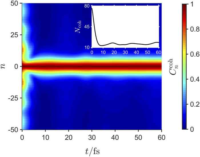
Figure 6: The time dependence of the exciton coherence correlation function, $C_{n}^{\textrm{coh}}$, Eq. (24). The time dependence of the associated coherence number, $N^{\textrm{coh}}$ (Eq. (25)), is shown in the inset. $N^{\textrm{coh}}$ decays within $10$ fs, i.e., within half a vibrational period. Reproduced from J. Chem. Phys. 148, 034901 (2018) with the permission of AIP publishing.

We emphasise that the prediction of an electron-polaron with short range correlations is a consequence of treating the phonons quantum mechanically, while the decay of exciton-site coherences is a consequence of the exciton and phonons being quantum mechanically entangled. Neither of these predictions are possible within the Ehrenfest approximation.

IV.2 Role of system-environment interactions

For an exciton to dissipate energy it must first couple to fast internal degrees of freedom (as described in the last section) and then these degrees of freedom must couple to the environment to expell heat. For a low-energy exciton (i.e., a LEGS) this process will cause adiabatic relaxation on a single potential energy surface, forming a VRSTretiak et al. (2002); Karabunarliev and Bittner (2003); Sterpone and Rossky (2008); De Leener et al. (2009). As shown in Fig. 3(a), however, for a kinetically hot exciton (i.e., a QEES) this relaxation is through a dense manifold of states and is necessarily a nonadiabatic interconversion between different potential energy surfaces. As already stated in Section II, the Ehrenfest approximation fails to correctly describe this process.

Dissipation of energy from an open quantum system arising from system-environment coupling is commonly described by a Lindblad master equationBreuer and Petruccione (2002)

$$\frac{\partial\hat{\rho}}{\partial{t}}=-\frac{i}{\hbar}\left[\hat{H},\hat{\rho}\right]-\frac{{\gamma}}{2}\sum_{n}\left(\hat{L}_{n}^{\dagger}\hat{L}_{n}\hat{\rho}+\hat{\rho}\hat{L}_{n}^{\dagger}\hat{L}_{n}-2\hat{L}_{n}\hat{\rho}\hat{L}_{n}^{\dagger}\right),$$ (26)

where $\hat{L}_{n}^{\dagger}$ and $\hat{L}_{n}$ are the Linblad operators, and $\hat{\rho}$ is the system density operator. In practice, a direct solution of the Lindblad master equation is usually prohibitively expensive, as the size of Liouville space scales as the square of the size of the associated Hilbert space. Instead, Hilbert space scaling can be maintained by performing ensemble averages over quantum trajectories (evaluated via the TEBD method), where the action of the Linblad dissipator is modeled by quantum jumps.Daley (2014)

In this section we assume that the C-C bond vibrations couple directly with the environmentMannouch, Barford, and Al-Assam (2018); Bednarz, Malyshev, and Knoester (2002), in which case the Linblad operators are the associated raising and lowering operators (i.e., $\hat{L}_{n}\equiv\hat{b}_{n}$, introduced in the last section). In addition,

$$\hat{H}=\hat{H}_{\text{FH}}+\frac{{\gamma}\hbar}{4}\sum_{n}\left(\hat{\tilde{Q}}_{n}\hat{\tilde{P}}_{n}+\hat{\tilde{P}}_{n}\hat{\tilde{Q}}_{n}\right).$$ (27)

(In Section V we discuss coupling of the torsional modes with the environmentAlbu and Yaron (2013).)

The ultrafast localization of exciton ODLRO (or exciton-site decoherence) described in Section IV.1 occurs via the coupling of the exciton to internal degrees of freedom, namely the C-C bond vibrations. We showed in Section III.3 (see Fig. 2(a)) that this coupling does not cause exciton density localization. However, dissipation of energy to the environment causes an exciton in a higher energy QEES to relax onto a lower energy LEGS (i.e., onto a chromophore) and thus the exciton density becomes localized.

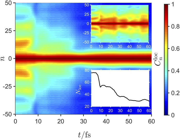
Figure 7: The time dependence of the exciton localization correlation function, $C^{\textrm{loc}}_{n}$ (Eq. (28)), for an initial high-energy QEES. The main figure corresponds to the time evolution with the dissipation time $T=\gamma^{-1}=100$ fs. The time dependence of the exciton density localization number, $N^{\textrm{loc}}$ (Eq. (29)), is given in the lower inset. The upper inset corresponds to the time evolution without external dissipation showing that in this case exciton denisty localization does not occur. Reproduced from J. Chem. Phys. 148, 034901 (2018) with the permission of AIP publishing.

The spatial extent of the exciton density, averaged over an ensemble of quantum trajectories, is quantified by the correlation functionSpano et al. (2008), approximated by

$$C_{n}^{\text{loc}}=\sum_{m}\left|\Psi_{m}\Psi_{m+n}^{*}\right|.$$ (28)

Fig. 7 shows the time dependence of $C_{n}^{\text{loc}}$ with an external dissipation time $T=\gamma^{-1}=100$ fs. The time scale for localization is seen from the time dependence of the exciton localization lengthTempelaar et al. (2014),

$$N_{\text{loc}}={\sum_{n}\left|n\right|C_{n}^{\text{loc}}}/{\sum_{n}C_{n}^{\text{loc}}},$$ (29)

which corresponds to the average distance between monomers for which the exciton wavefunction overlap remains non-zero, and is given in the lower inset of Fig. 7. Evidently, the coupling to the environment - and specifically, the damping rate - controls the timescale for energy relaxation and exciton density localization onto chromophores. In contrast, the upper inset to Fig. 7 shows an absence of localization without external dissipation, indicating that exciton density localization is an extrinsic process.

Figure 7 is obtained by averaging over an ensemble of trajectories. To understand the physical process of localization onto a chromophore, Fig. 8 illustrates the exciton density of a single quantum trajectory for a photoexcited QEES (shown in Fig. 2(b)). At a time ca. 20 fs a ‘quantum jump’ caused by the stochastic application of a Lindblad jump operator causes the exciton to localize onto the $j=2$ LEGS, shown in Fig. 2(a), i.e., the high-energy extended state has randomly localized onto a chromophore because of a ‘measurement’ by the environment.

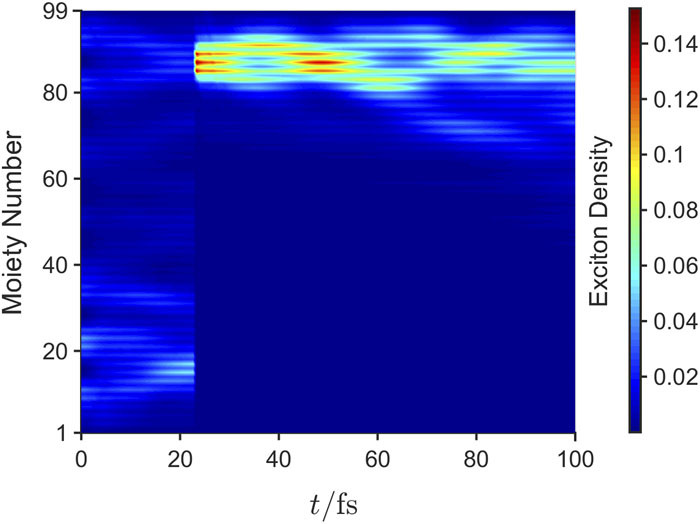
Figure 8: The time dependence of the exciton density for a single trajectory of the quantum jump trajectory method. The discontinuity in the density at ca. 20 fs is a ‘quantum jump’ caused by the stochastic application of a Lindblad jump operator. The dynamics were performed for an initial high energy QEES given in Fig. 2(b), showing localization onto the LEGSs (i.e., a chromophore) labeled $j=2$ in Fig. 2(a). Reproduced from J. Chem. Phys. 148, 034901 (2018) with the permission of AIP publishing.

IV.3 Role of slow bond rotations

By dissipating energy into the environment on sub-ps timescales, hot excitons relax into localized LEGSs, i.e., onto chromophores. The final intrachain relaxation and localization process now takes place, namely exciton-polaron formation via coupling to the torsional degrees of freedom. For this relaxation to occur bond rotations must be allowed, which means that this process is highly dependent on the precise chemical structure of the polymer and its environment.

Assuming that bond rotations are not sterically hindered, their coupling to the excitons is conveniently modeled (via Eq. (7) and Eq. (12)) by supplementing the Frenkel-Holstein model (i.e., Eq. (IV.1)) byBarford and Mannouch (2018)

$$\hat{H}_{\textrm{rot}}=-\sum_{n=1}^{N-1}B(\theta_{n}^{0})\times({\phi}_{n+1}-{\phi}_{n})\hat{T}_{n,n+1}+\frac{1}{2}\sum_{n=1}^{N}\left(K_{\textrm{rot}}{\phi}_{n}^{2}+{L}_{n}^{2}/I\right).$$

Here, ${\phi}$ is the angular displacement of a monomer from its groundstate equilibrium value and ${L}$ is the associated angular momentum of a monomer around its bridging bonds.

The first term on the right-hand-side of Eq. (IV.3) indicates that the change in the dihedral angle, $\Delta{\theta}_{n}=({\phi}_{n+1}-{\phi}_{n})$, couples linearly to the bond-order operator, $\hat{T}_{n,n+1}$, where

$$B(\theta_{n}^{0})=J_{SE}\sin 2\theta_{n}^{0}$$ (31)

is the exciton-roton coupling constant and $\theta_{n}^{0}$ is the groundstate dihedral angle for the $n$th bridging bond. The final term is the sum of the elastic and kinetic energies of the rotational harmonic oscillator.

The natural angular frequency of oscillation is $\omega_{\textrm{rot}}=(K_{\textrm{rot}}/I)^{1/2}$, where $K_{\textrm{rot}}$ is the elastic constant of the rotational oscillator and $I$ is the moment of inertia, respectively. As discussed in Section III.3.1, $K_{\textrm{rot}}$ is larger for the bridging bond in the excited state than the groundstate, because of the increase in bond order. Also notice that both the moment of inertia (and thus $\omega_{\textrm{rot}}$) of a rotating monomer and its viscous damping from a solvent are strongly dependent on the side groups attached to it. As discussed in the next section, this observation has important implications for whether the motion is under or over damped and on its characterstic timescales.

Unlike C-C bond vibrations, being over 10 times slower torsional oscillations can be treated classicallyBarford and Mannouch (2018). Furthermore, since we are now concerned with adiabatic relaxation on a single potential energy surface, we may employ the Ehrenfest approximation. Thus, using Eq. (IV.3), the torque on each ring is

$$\Gamma_{n} = -\frac{\partial\langle\hat{H}_{rot}\rangle}{\partial{\phi}_{n}}$$ (32)

$$= -K_{\textrm{rot}}{\phi}_{n}+\lambda_{n}$$

where we define

$$\lambda_{n}=B(\theta_{n-1}^{0})\langle\hat{T}_{n-1,n}\rangle-B(\theta_{n}^{0})\langle\hat{T}_{n,n+1}\rangle.$$ (33)

Setting $\Gamma_{n}=0$ gives the equilibrium angular displacements in the excited state as ${\phi}_{n}^{\textrm{eq}}=\lambda_{n}/K_{\textrm{rot}}$. ${\phi}_{n}$ is subject to the Ehrenfest equations of motion,

$$I\frac{d{\phi}_{n}}{d{t}}={L}_{n},$$ (34)

and

$$\frac{d{L}_{n}}{d{t}} =\Gamma_{n}-\gamma L_{n},$$ (35)

where the final term represents the damping of the rotational motion by the solvent.

IV.3.1 A single torsional oscillator

Before considering a chain of torsional oscillators, it is instructive to review the dynamics of a single, damped oscillator subject to both restoring and displacement forces. The equation of motion for the angular displacement is

$$\frac{d^{2}\phi(t)}{dt^{2}}=-\omega_{\textrm{rot}}^{2}(\phi(t)-\phi_{\textrm{eq}})-\gamma\frac{d\phi(t)}{dt,}$$ (36)

where $\phi_{\textrm{eq}}=\lambda/K_{rot}$ is proportional to the displacement force.

In the underdamped regimeFrench (1971), defined by $\gamma<2\omega_{\textrm{rot}}$,

$$\phi(t)=\phi_{\textrm{eq}}\left(1-\cos(\omega t)\exp(-\gamma t/2)\right),$$ (37)

where $\omega=(\omega_{\textrm{rot}}^{2}-\gamma^{2}/4)^{1/2}$. In this regime, the torsional angle undergoes damped oscillations with a period $T=2\pi/\omega$ and a decay time $\tau=2/\gamma$.

Conversely, in the overdamped regimeFrench (1971), defined by $\gamma>2\omega_{\textrm{rot}}$,

$$\phi(t)=\phi_{\textrm{eq}}\left(1-\frac{1}{4\beta}\left(\gamma_{1}\exp(-\gamma_{2}t/2)-\gamma_{2}\exp(-\gamma_{1}t/2)\right)\right),$$

where $\gamma_{1}=\gamma+2\beta$, $\gamma_{2}=\gamma-2\beta$ and $\beta=(\gamma^{2}/4-\omega_{\textrm{rot}}^{2})^{1/2}$. Now, the torsional angle undergoes damped biexponential decay with the decay times $\tau_{1}=2/\gamma_{1}$ and $\tau_{2}=2/\gamma_{2}$. In the limit of strong damping, i.e., $\gamma\gg 2\omega_{\textrm{rot}}$, there is a fast relaxation time $\tau_{1}=1/\gamma=\tau/2$ and a slow relaxation time $\tau_{2}=\gamma/\omega_{\textrm{rot}}^{2}\gg\tau$. In this limit, as the slow relaxation dominates at long times, the torsional angle approaches equilibrium with an effective mono-exponential decay.

For a polymer without alkyl side groups, e.g., PPP and PPV, $\omega_{\textrm{rot}}\sim\gamma\sim 10^{13}$ s^-1 and are thus in the underdamped regime with sub-ps relaxation. However, polymers with side groups, e.g., P3HT, MEH-PPV and PFO, have a rotational frequency up to ten times smaller and a larger damping rate, and are thus in the overdamped regimeWells and Blank (2008).

IV.3.2 A chain of torsional oscillators

An exciton delocalized along a polymer chain in a chromophore couples to multiple rotational oscillators resulting in collective oscillator dynamics. Eq. (31) and Eq. (33) indicate that torsional relaxation only occurs if the monomers are in a staggered arrangement in their groundstate, i.e., $\theta_{n}^{0}=(-1)^{n}\theta^{0}$. In this case the torque acts to planarize the chain. Furthermore, since the torsional motion is slow, the self-trapped exciton-polaron thus formed is ‘heavy’ and in the under-damped regime becomes self-localized on a timescale of a single torsional period, i.e., $200-600$ fs. In this limit the relaxed staggered bond angle displacement mirrors the exciton density. Thus, the exciton is localized precisely as for a ‘classical’ Landau polaron and is spread over $\sim 10$ monomersBarford and Mannouch (2018).

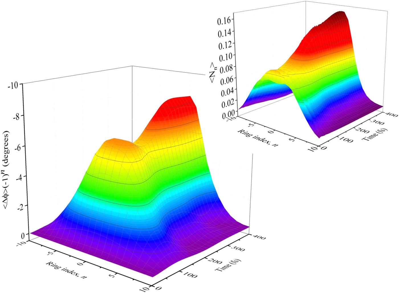
Figure 9: The time-evolution of the staggered angular displacement, $\langle{\phi}_{n}\rangle\times(-1)^{n}$. The change of dihedral angle is $\Delta\theta_{n}=(\phi_{n+1}-\phi_{n})$, showing local planarization for a PPP chain of 21 monomers. The inset displays the time-evolution of the exciton density, $\langle N_{n}\rangle$, showing exciton density localization after a single torsional period ($\sim 200$ fs). In the long-time limit (i.e., $t\gtrsim 400$ fs) $\langle{\phi}_{n}\rangle\propto\langle N_{n}\rangle\times(-1)^{n}$, illustrating classical (Landau) polaron formation. Reproduced from J. Chem. Phys. 149, 214107 (2018) with the permission of AIP publishing.

The time-evolution of the staggered angular displacement, $\langle{\phi}_{n}\rangle\times(-1)^{n}$, is shown in Fig. 9 illustrating that these displacements reach their equilibrated values after two torsional periods (i.e., $t\gtrsim 400$ fs). The inset also displays the time-evolution of the exciton density, $\langle N_{n}\rangle$, showing exciton density localization after a single torsional period ($\sim 200$ fs).

So far we have described how exciton coupling to torsional modes causes a spatially varying planarization of the monomers that acts as a one-dimensional potential which self-localizes the exciton. The exciton ‘digs a hole for itself’, forming an exciton-polaronLandau (1933). Some researchersWestenhoff et al. (2006), however, argue that torsional relaxation causes an exciton to become more delocalized. A mechanism that can cause exciton delocalization occurs if the disorder-induced localization length is shorter than the intrinsic exciton-polaron size. Then, in this case for freely rotating monomers, the stiffer elastic potential in the excited state causes a decrease both in the variance of the dihedral angular distribution, $\sigma_{\theta}^{2}=k_{B}T/K_{\textrm{rot}}$, and the mean dihedral angle, $\theta_{0}$. This, in turn, means that the exciton band width, $|4J|$, increases and the diagonal disorderMarcus, Tozer, and Barford (2014), $\sigma_{J}=J_{SE}\sigma_{\theta}\sin 2\theta_{0}$, decreases. Hence, the disorder-induced localization, $L_{\textrm{loc}}\sim(|J|/\sigma_{J})^{2/3}$, increases (see Section III.2).

IV.4 Summary

The conclusions that we draw from the previous three sections are that a band edge excitation (i.e., a LEGS, which is an exciton spanning a single chromophore) undergoes ultrafast exciton site decoherence via its coupling to fast C-C bond stretches. It subsequently couples to slow torsional modes causing planarization and exciton density localization on the chromophore. A hot exciton (i.e., a QEES) also undergoes ultrafast exciton site decoherence. However, exciton density localization within a chromophore only occurs after localization onto the chromophore via a stochastic interaction with the environment.

IV.5 Time resolved fluorescence anisotropy

For general polymer conformations, the loss of ODLRO (or the localization of the exciton coherence function) causes a reduction and rotation of the transition dipole moment. The rotation is quantified by the fluorescence anisotropy, defined byLakowicz (2006)

$$r=\frac{I_{\parallel}-I_{\perp}}{I_{\parallel}+2I_{\perp}},$$ (39)

where $I_{\parallel}$ and $I_{\perp}$ are the intensities of the fluorescence radiation polarised parallel and perpendicular to the incident radiation, respectively.

For an arbitrary state of a quantum system, $|\Psi\rangle$, the integrated fluorescence intensity polarised along the $x$-axis is related to the $x$ component of the transition dipole operator, $\hat{\mu}_{x}$, by

$$I_{x}\propto\sum_{v}\left|\langle\Psi|\hat{\mu}_{x}|\textrm{GS},v\rangle\right|^{2},$$ (40)

where $|\textrm{GS},v\rangle$ corresponds to the system in the ground electronic state, with the nuclear degrees of freedom in the state characterised by the quantum number $v$.

The averaged fluorescence anisotropy is defined by

$$\langle r\left(t\right)\rangle=0.4\times\frac{\sum_{i}I_{i}\left(t\right)r_{i}\left(t\right)}{\sum_{i}I_{i}\left(t\right)},$$ (41)

where $I_{i}\left(t\right)$ is the total fluorescence intensity and $r_{i}\left(t\right)$ is the fluorescence anisotropy, associated with a particular conformation $i$ at time $t$. The factor of 0.4 is included on the assumption that the polymers are oriented uniformly in the bulk material.Lakowicz (2006) Fig. 10 shows the simulated $\langle r\left(t\right)\rangle$ for both a high energy QEES and a low energy LEGS for an ensemble of conformationally disordered polymers.

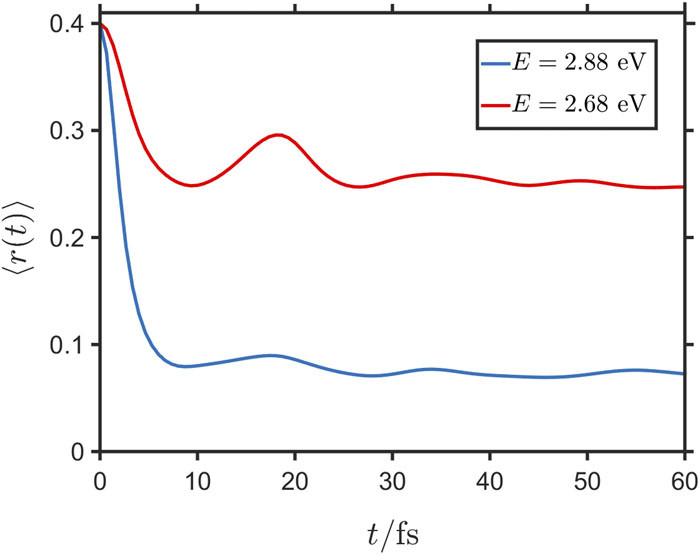
Figure 10: The time dependence of the fluorescence anisotropy, $\langle r\left(t\right)\rangle$, for two initial Frenkel excitons coupled to C-C bond stretches. The red curve corresponds to an initial LEGS, while the blue curve corresponds to a QEES. Reproduced from J. Chem. Phys. 148, 034901 (2018) with the permission of AIP publishing.

Figure 11: The experimental time dependence of the fluorescence anisotropy, $\langle R\left(t\right)\rangle$, in polythiophene in solution. $\langle R\left(t\right)\rangle$ has decayed from $0.4$ to $\sim 0.25$ within 10 fs, consistent with the theoretical predictions shown in Fig. 10. Subsequent fluorescence depolarization is caused by slower torsional relaxation on timescales of $1-10$ ps followed by possible conformational changesWells et al. (2007). Reproduced from J. Phys. Chem. C 111, 15404 (2007) with the permission of ACS publishing.

It is instructive to express Eq. (40) as

$$I_{x}\propto\sum_{m,n}s_{m}^{x}s_{n}^{x}\rho_{mn},$$ (42)

where $s^{x}_{m}$ is the $x$-component of the unit vector for the $m$th monomer and $\rho_{mn}$ is the exciton reduced density matrix. Then, using Eq. (24), Eq. (25), and Eq. (42), we observe that the emission intensity, $I_{x}$, is related to the coherence length, $N^{\textrm{coh}}$. Thus, not surprisingly, the dynamics of $\langle r\left(t\right)\rangle$ resembles that of $N^{\textrm{coh}}(t)$ shown in Fig. 6. In particular, we observe a loss of fluorescence anisotropy within 10 fs, mirroring the reduction of $N^{\textrm{coh}}$ in the same time. Furthermore, since there is greater exciton coherence localization for the QEES than for the LEGS, the former exhibits a greater loss of anisotropy. This predicted loss of fluorescence anisotropy within 10 fs has been observed experimentally, as shown in Fig. 11. Slower sub-ps decay of anisotropy occurs because of exciton density localization via coupling to torsional modes.

V Intrachain Exciton Motion

The last section described the relaxation and localization of higher energy excited states onto chromophores, and the subsequent torsional relaxation and localization on the chromophore. We now consider the relaxation and dynamics of these relaxed excitons caused by the stochastic torsional fluctuations experienced by a polymer in a solvent.

Environmentally-induced intrachain exciton relaxation in poly(phenylene ethynylene) was modeled by Albu and YaronAlbu and Yaron (2013) using the Frenkel exciton model supplemented by the torsional degrees of freedom, i.e., $\hat{H}=\hat{H}_{F}+\hat{H}_{rot}$ (given by Eq. (2) and Eq. (IV.3), respectively). Fast vibrational modes were neglected because although they cause self-trapping, they do not cause self-localization, and these modes can be assumed to respond instantaneously to the torsional modes. The polymer-solvent interactions were modeled by the Langevin equation. For chains longer than the exciton localization length the excited-state relaxation showed biexponential behavior with a shorter relaxation time of a few ps and a longer relaxation time of tens of ps.

After photoexcitation of the $n=2$ (charge-transfer) exciton in oligofluorenes, Clark et al.Clark et al. (2012) reported torsional relaxation on sub-100 fs timescales. Since this timescale is faster than the natural rotational period of an undamped monomer, they ascribed it to the electronic energy being rapidly converted to kinetic energy via nonadiabatic transitions. They argue that this is analogous to inertial solvent reorganization.

Tozer and BarfordTozer and Barford (2015) using the same model as Albu and Yaron to model intrachain exciton motion in PPP where the exciton dynamics were simulated on the assumption that at time $t+\delta t$ the new exciton target state is the eigenstate of $\hat{H}(t+\delta t)$ with the largest overlap with the previous target state at time $t$.

A more sophisticated simulation of exciton motion in poly(p-phenylene vinylene) and oligothiophenes chains was performed by Burghardt and coworkersBinder and Burghardt ; Binder et al. ; Binder and Burghardt (2020); Hegger, Binder, and Burghardt (2020) where high-frequency C-C bond stretches were also included, the solvent was modeled by a set of harmonic oscillators with an Ohmic spectral density, and the system was evolved via the multilayer-MCTDH method. Their results, however, are in quantitative agreement with those of Tozer and Barford in the ‘low-temperature’ limit (discussed in Section V.3), namely activationless, linearly temperature-dependent exciton diffusion with exciton diffusion coefficients larger, but close to experimental values.

The Brownian forces excerted by the solvent on the polymer monomers have two consequences. First, as already noted in Section III.2, the instantaneous spatial dihedral angle fluctuations Anderson localize the Frenkel center-of-mass wavefunction. Second, the temporal dihedral angle fluctuations cause the exciton to migrate via two distinct transport processes.

At low temperatures there is small-displacement adiabatic motion of the exciton-polaron as a whole along the polymer chain, which we will characterize as a ‘crawling’ motion. At higher temperatures the torsional modes fluctuate enough to cause the exciton to be thermally excited out of the self-localized polaron state into a more delocalized LEGS or quasi-band QEES. While in this more delocalized state, the exciton momentarily exhibits quasi-band ballistic transport, before the wavefunction ‘collapses’ into an exciton-polaron in a different region of the polymer chain. We will characterize this large-scale displacement as a non-adiabatic ‘skipping’ motion.

Before describing the details of these types of motion, we first describe a model of solvent dynamics and consider again exciton-polaron formation in a polymer subject to Brownian fluctuations.

V.1 Solvent dynamics

If the solvent molecules are subject to spatially and temporally uncorrelated Brownian fluctuations, then the monomer rotational dynamics are controlled by the Langevin equation

$$\frac{dL_{n}(t)}{dt}=\Gamma_{n}(t)+R_{n}(t)-\gamma L_{n}(t),$$ (43)

where $\Gamma_{n}(t)$ is the systematic torque given by Eq. (32). $R_{n}(t)$ is the stochastic torque on the monomer due to the random fluctuations in the solvent and $\gamma$ is the friction coefficient for the specific solvent. From the fluctuation-dissipation theorem, the distribution of random torques is given by

$$\langle R_{m}(t)R_{n}(0)\rangle=2I\gamma k_{B}T\delta_{mn}\delta(t),$$ (44)

which are typically sampled from a Gaussian distribution with a standard deviation of $\sigma_{R}=(2I\gamma k_{B}T)^{\frac{1}{2}}$. As a consequence of these Brownian fluctuations the monomer rotations are characterized by the autocorrelation functionNitzan (2006)

$$\langle\delta\phi(t)\delta\phi(0)\rangle=$$

$$\langle\delta\phi^{2}\rangle\left(\cos(\omega_{rot}t)+\left(\frac{\gamma}{2\omega_{rot}}\right)\sin(\omega_{rot}t)\right)\exp(-\gamma t/2),$$ (45)

where $\langle\delta\phi^{2}\rangle={k_{B}T}/{K_{rot}}$, $K_{rot}$ is the stiffness and $\omega_{rot}=\sqrt{K_{rot}/I}$ is the angular frequency of the torsional mode.

V.2 Polaron formation

As we saw in Section IV.3, at zero temperature torsional modes couple to the exciton, forming an exciton-polaron. At finite temperatures, however, a combination of factors affect the localization of the exciton. First, the exciton will still attempt to form a polaron. However, the thermally induced fluctuations in the torsional angles will affect the size of this exciton-polaron, as there is a non-negligible probability that the exciton will be excited out of its polaron potential well into a more delocalized state at high enough temperatures. Second, the exciton states will be Anderson localized by the instantaneous torsional disorder.

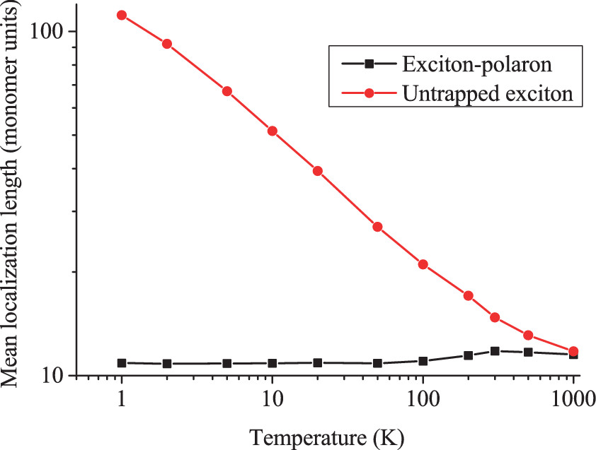
Figure 12: The exciton localization length as a function of temperature for the ‘free’ (i.e., ‘untrapped’) exciton (red circles) and exciton-polaron (i.e., ‘self-trapped’) (black squares). The untrapped exciton localization length obeys $L_{\textrm{loc}}^{\textrm{free}}\propto T^{-1/3}$. The lengths coincide when $k_{B}T\sim$ the exciton-polaron binding energy. Reproduced from J. Chem. Phys. 143, 084102 (2015) with the permission of AIP publishing.

Fig. 12 shows how the average localization length varies with temperature both with and without coupling between the exciton and the torsional modes (i.e., ‘self-trapped’ and ‘free’ exciton, respectively). As described in Section III.2, the localization length for the ‘free’ exciton is determined by Anderson localization. For small angular displacements from equilibrium a Gaussian distribution of dihedral angles implies a Gaussian distribution of exciton transfer integrals. Then, as confirmed by the simulation results shown in Fig. 12, from single-parameter scaling theory, $L_{\textrm{loc}}^{\textrm{free}}\propto\sigma_{\theta}^{-2/3}=\langle\delta\theta^{2}\rangle^{-1/3}\propto T^{-1/3}$.

In contrast, the localization length of the ‘self-trapped’ exciton slowly increases with temperature because of the thermal excitation of the exciton from the self-localized polaron to a more delocalized LEGS or QEES. The two values coincide when $k_{B}T$ equals the exciton-polaron binding energy (i.e., $T\sim 1500$ K in PPP).

V.3 Adiabatic ‘crawling’ motion

At low temperatures ($\lesssim 100$ K) the exciton has only a small amount of thermal energy, and not enough to regularly break free from its polaronic torsional distortions. Thus, the exciton-polaron migrates quasi-adiabatically and diffusively as a single unit. This is a collective motion of the exciton and the torsional degrees of freedom, as the torsional planarization accompanies the exciton. The random walk motion is illustrated in Fig. 13, which shows that the mean-square-distance traveled by the exciton-polaron is proportional to time, i.e., $\langle L^{2}\rangle=2D_{A}(T)t$, where $D_{A}$ is the diffusion coefficient. Since the migration of the exciton-polaron is an activationless process, as the gradients of Fig. 13 indicate, at low temperatures it obeys the Einstein-Smoluchowski equation, $D_{A}(T)=\mu k_{B}T$, where $\mu$ is the mobility of the particle.

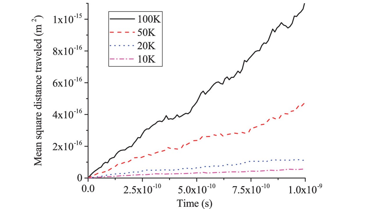
Figure 13: The intrachain mean-square-distance traveled by an exciton-polaron at low temperatures caused by stochastic torsional fluctuations. The motion is diffusive, as shown by the mean-square-distance increasing linearly with time: $\langle L^{2}\rangle=2D_{A}(T)t$. The gradients satisfy the Einstein-Smoluchowski equation, $D_{A}(T)=\mu k_{B}T$. Reproduced from J. Chem. Phys. 143, 084102 (2015) with the permission of AIP publishing.

The time taken for an exciton to diffuse a distance $L$ along the chain is determined by the equation for a one-dimensional random walk, i.e., $\tau_{D}=\langle L^{2}\rangle/2D$. As shown in Fig. 12, the typical exciton-polaron localization length is $\sim 12$ monomers or $\sim 6$ nm in PPP. This characteristic length scale implies a characteristic timescale, namely the time taken for the exciton to diffuse along a chromophore length. As shown in Table 3, these timescales are typically $3-30$ ps at room temperature depending on the solvent friction coefficient, being shorter at higher temperatures and smaller damping rates. As we show in Section V, these timescales are an order of magnitude shorter than Förster transfer times in the condensed phase.

As the exciton-polaron migrates along the polymer chain it experiences a different potential energy landscape, so its energy will also fluctuate on a timescale $\sim\tau_{D}$. Interestingly, these timescales are consistent with the longer timescale found experimentally in biexponential fits of relaxation processes of polymers in solution (see Table I) and correspond to the longer timescale simulated by Albu and YaronAlbu and Yaron (2013) in longer polymers.

$\gamma$ (s-1)	$T$ (K)	$D_{A}$ ($\textrm{cm}^{2}\textrm{ s}^{-1}$)	$\tau_{D}$ (ps)
$10^{11}$	300	$6.0\times 10^{-2}$	3.0
$10^{11}$	100	$2.0\times 10^{-2}$	9.0
$10^{12}$	300	$2.7\times 10^{-2}$	6.7
$10^{12}$	100	$9.0\times 10^{-3}$	20
$10^{13}$	300	$6.0\times 10^{-3}$	30
$10^{13}$	100	$2.0\times 10^{-3}$	90

Table 3: Calculated intrachain adiabatic exciton diffusion coefficients, $D_{A}$, and times, $\tau_{D}$, in PPP from refTozer and Barford (2015). $\tau_{D}$ is the time taken for an exciton to diffuse along a chromophore of linear size $6$ nm in a solvent at temperature, $T$, with a damping rate $\gamma$. From simulationsTozer and Barford (2015), $\tau_{D}\sim\gamma^{1/2}/T$. Hegger et al.Hegger, Binder, and Burghardt (2020) obtained $D_{A}\sim 10^{-2}$ $\textrm{cm}^{2}\textrm{ s}^{-1}$ in oligothiophenes at 300 K and $\gamma=5\times 10^{12}$ s^-1.

V.4 Nonadiabatic ‘skipping’ motion

At higher temperatures, adiabatic ‘crawling’ migration of the exciton-polaron, as described above, still occurs. However, a second non-adiabatic mechanism for the dynamics plays an important role. This mechanism involves the exciton-polaron being excited to a high enough energy by the thermal fluctuations to be excited out of the polaron potential well, resulting in a breakdown of the polaron and the exciton to enter an untrapped local exciton ground state (LEGS), or a higher energy quasi-extended exciton state (QEES). Once in this more delocalized state the exciton has quasi-band characteristics and travels quasi-ballistically.

As described in Section IV, however, on a sub-ps timescale the hot exciton will shed some of its excess kinetic energy and relax back into an exciton-polaron. As a result, the time-averaged exciton localization length calculations of Fig. 12 show only a slight increase in localization length with increasing temperatures, as the majority of its lifetime is still spent in self-localized exciton-polarons.

The requirement that the exciton is excited out of the polaron potential well means that this process is activated. Thus, from a simple Fermi golden rule analysis it can be shown thatBarford and Tozer (2014)

$$D_{NA}(T)\sim T^{2/3}\exp\Bigg{(}-\frac{\Delta E}{k_{B}T}\Bigg{)},$$ (46)

where $\Delta E$ is the exciton-polaron binding energy. At 300 K $D_{NA}$ is approximately twice as large as $D_{A}$ and thus the overall diffusion coefficient is considerably enhanced by this skipping motion.

The role of exciton transport in disordered one-dimensional systems via higher-energy quasi-band states has been discussed in refBednarz, Malyshev, and Knoester (2002), where in that work phonons in the condensed phase environment induced non-adiabatic transitions.

VI Interchain Exciton Motion

The stochastic, torsionally-induced intrachain exciton diffusion in polymers in solution described in the last section is not expected to be the primary cause of exciton diffusion in polymers in the condensed phase. Instead, owing to restricted monomer rotations and the proximity of neighboring chains, exciton transfer is determined by Coulomb-induced, Förster-like processes. Moreover, since dissipation rates are typicallySterpone and Rossky (2008); De Leener et al. (2009) $10^{12}-10^{13}$ s^-1, whereas exciton transfer rates are typically $10^{9}-10^{11}$ s^-1, exciton migration is an incoherent or diffusive processHwang and Scholes (2011).

Early models of condensed phase diffusion assumed that the donors and acceptors are point-dipoles whose energy distribution is a Gaussian random variableMovaghar et al. (1986); Movaghar, Ries, and Grunewald (1986); Meskers et al. (2001). An advantage of these models is that they allow for analytical analysis, for example predicting how the diffusion length varies with disorder and temperatureAthanasopoulos, Bässler, and Köhler (2019). They also reproduce some experimental features, such as the time-dependence of spectral diffusion. A disadvantage, however, is that there is no quantitative link between the model and actual polymer conformations and morphology.

More recent approaches have attempted to make the link between random polymer conformations and the energetic and spatial distributions of the donors and acceptors via the concept of extended chromophoresBeljonne et al. (2002); Hennebicq et al. (2005); Athanasopoulos et al. (2008); Singh et al. (2009) and using transition densities to compute transfer integrals. However, the usual practice has been to arbitrarily define chromophores via a minimum threshold in the $p$-orbital overlaps, and then obtain a distribution of energies by assuming that the excitons delocalize freely on the chromophores thus defined as a ‘particle-in-a-box’.

As discussed in Section III.2, an unambiguous link between polymer conformations and chromophores may be made by defining chromophores via the spatial extent of local exciton ground states (LEGSs). Using this insight, a more realistic first-principles model that accounts for polymer conformations can be developedBarford, Bittner, and Ward (2012); Barford and Tozer (2014). This is described in Section VI.1, while its predictions and comparisons to experimental observations are described in Section VI.2.

VI.1 Modified Förster theory

The Förster exciton transfer rate from a donor (D) to an acceptor (A) has the general Golden rule form

$$k_{DA}=\left(\frac{2\pi}{\hbar}\right)\left|J_{DA}\right|^{2}\int D(E)A(E)dE,$$ (47)

where $J_{DA}$ is the Coulomb-induced donor-acceptor transfer integral defined by Eq. (3). As we remarked in Section III.1, the transition density vanishes for odd-parity singlet excitons; it also vanishes for all triplet excitons.

$D(E)$ and $A(E)$ are the donor and acceptor spectral functions, respectively, defined by

$$D(E)=\sum_{v}F_{0v}^{D}\delta(E+{E}^{D}_{0v})$$ (48)

and

$$A(E)=\sum_{v}F_{0v}^{A}\delta(E-{E}^{A}_{0v}),$$ (49)

where $F_{0v}$ is the effective Franck-Condon factor, defined in Eq. (51). $E^{A}_{0v}=(E^{A}_{00}+v\hbar\omega_{vib})$ is the excitation energy of the acceptor, while $E^{D}_{0v}=-(E^{D}_{00}-v\hbar\omega_{vib})$ is the de-excitation energy of the donor.

The link between actual polymer conformations and a realistic model of exciton diffusion is made by realising that the donors and acceptors for exciton transfer are LEGSs (i.e., chromophores). This assumption is based on the observation that exciton transfer occurs at a much slower rate than state interconversion, so the donors are LEGSs, while the spectral overlap between LEGSs and higher energy QEESs is small, so the acceptors are also LEGSs. Moreover, the energetic and spatial distribution of LEGSs is entirely determined by the conformational and site disorder, as described in Section III.2. Finally, polaronic effects are incorporated by an effective Huang-Rhys factor for each chromophore and the Condon approximation may be assumed as C-C vibrational modes do not cause exciton self-localization.

Then, as proved rigorously in refBarford and Tozer (2014):

1. $J_{DA}$ is evaluated by invoking the Condon approximation and using the line-dipole approximationBarford (2013a, 2007)

   $$J_{DA}=\left(\frac{1}{4\pi\varepsilon_{r}\varepsilon_{0}}\right)\sum_{\begin{subarray}{c}n\in D\\ n^{\prime}\in A\end{subarray}}\frac{\kappa_{nn^{\prime}}}{R_{nn^{\prime}}^{3}}\mu_{D}\Psi_{D}(n)\mu_{A}\Psi_{A}(n^{\prime}),$$ (50)

   where $\Psi(n)$ is the LEGS center-of-mass wavefunction on monomer $n$ determined from the disordered Frenkel exciton model (Eq. (2)). Since the spatial extent of $\Psi(n)$ defines a chromophore, the sum over $n$ and $n^{\prime}$ is implicitly over monomers of a donor and acceptor chromophore, respectively. $\mu_{X}$ is the transition dipole moment of a single monomer of the donor ($X=D$) or acceptor ($X=A$) chromophores (so $\mu_{X}\Psi_{X}(n)$ is the transition dipole moment of monomer $n$ as part of the chromophore). $\kappa_{nn^{\prime}}$ is the orientational factor, defined in Eq. (5), and $R_{nn^{\prime}}$ is the separation of monomers on the donor and acceptor chromophores. The line-dipole approximation is valid when the monomer sizes are much smaller than their separation on the donor and acceptor chromophores; it becomes the point-dipole approximation when the chromophore sizes are much smaller than their separation.

2. The spectral functions describe ‘polaronic’ effects, by containing effective Franck-Condon factors which describe the chromophores coupling to effective modes with reduced Huang-Rhys parameters:

   $$F_{0v}=\frac{S_{\textrm{eff}}^{v}\exp(-S_{\textrm{eff}})}{v!},$$ (51)

   where $S_{\textrm{eff}}=S/\textrm{PN}$, $S$ is the local Huang-Rhys parameter (defined by Eq. (22)) and $\textrm{PN}=\left(\sum_{n}|\Psi_{n}|^{4}\right)^{-1}$ is the participation number (or size) of the chromophoreBarford and Marcus (2014).

3. Similarly, the $0-0$ transition energy is defined by $E_{00}=(E^{\textrm{vert}}-E^{\textrm{relax}})$, where $E^{\textrm{vert}}$ is determined from the Frenkel exciton model and $E^{\textrm{relax}}=\hbar\omega S_{\textrm{eff}}$ is the effective reorganisation energy for the effective mode.

VI.2 Condensed-phase exciton diffusion

We might attempt to anticipate the results of the simulation of exciton diffusion from the properties of the exciton transfer rate, $k_{DA}$. When the chromophore size, $L$, is much smaller than the donor-acceptor separation, $R$, the point-dipole approximation is valid. In this limit $k_{DA}\sim L^{2}/R^{6}$ and thus the hopping rate increases with increasing chromophore size. Conversely, when the chromophore size is much larger than the donor-acceptor separation, the line-dipole approximation predicts that for straight, parallel or collinear chromophoresWong, Bagchi, and Rossky (2004); Das and Ramasesha (2010); Barford (2010) $k_{DA}\sim 1/(LR)^{2}$ and thus the hopping rate decreases with increasing chromophore size.

In practice, Monte Carlo simulations assuming a statistical model of polymer conformations find that the exciton hopping rate is essentially independent of disorder and hence of chromophore size. This is presumably because neither the assumption of straight, parallel chromophores nor point dipoles are valid. These simulations also show that the average time taken for the first exciton hop to occur after photoexcitation is $\sim 10$ ps, whereas the time intervals between hops just prior to radiative recombination is over 10 times longer, and indeed becoming so long that a radiative transition is competitive. This increase in hopping time intervals occurs because as an exciton diffuses through the polymer system it continuously looses energy. Thus, the energetic condition for exciton transfer to occur, namely $E_{A}\leq E_{D}$, becomes harder to satisfy and in general the spectral overlap between the donor and acceptor decreases. As the excitons diffuse they eventually become trapped in ‘emissive’ chromophores, from which they radiate. As shown in Fig. 14, these emissive chromophores occupy the low energy tail of the LEGSs density of states. Their quasi-Gaussian distribution explains spectral diffusionHayes, Samuel, and Phillips (1995); Meskers et al. (2001): a time-dependent change in the fluorescence energy, satisfying $E\propto-\log t$.

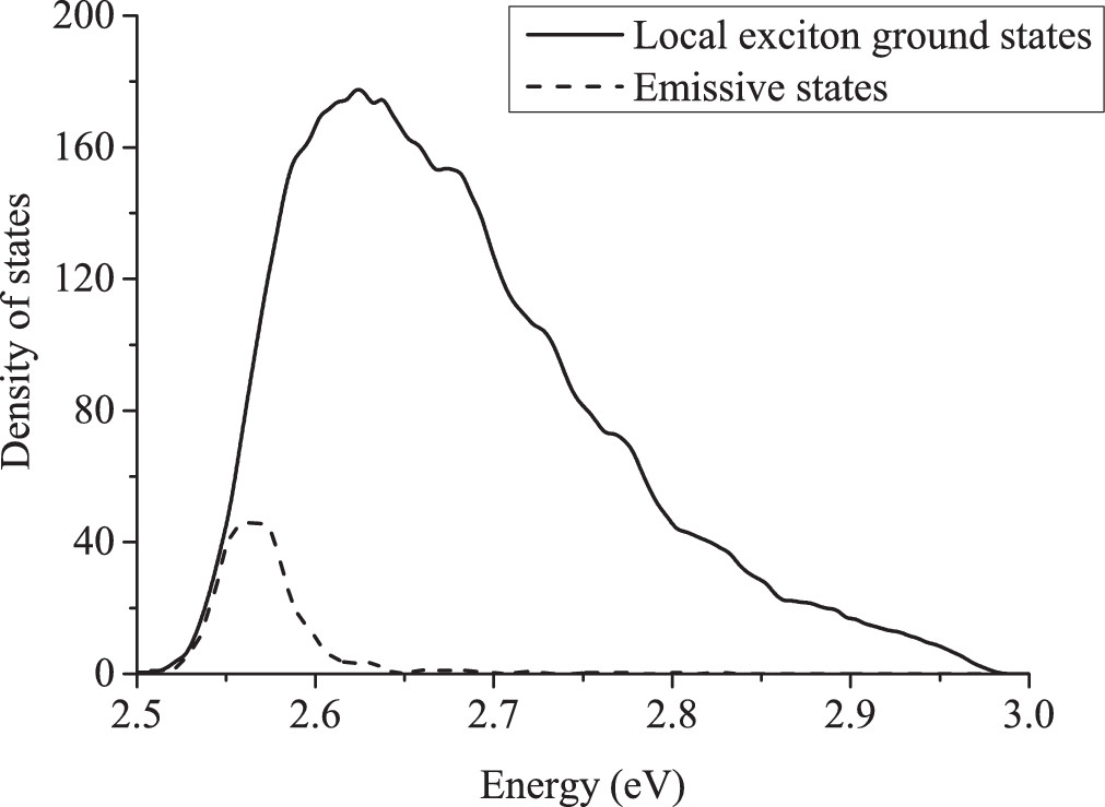
Figure 14: The density of states for absorbing LEGSs (solid line) and emitting trap states (dashed line) for an ensemble of PPV chains, with a Gaussian distribution of dihedral angles. $\langle\theta_{0}\rangle=10^{0}$, $\sigma_{\theta_{0}}=5^{0}$, and $\sigma_{\theta}=5^{0}$. Reproduced from J. Chem. Phys. 141, 164103 (2014) with the permission of AIP publishing.

Typically, the average hop distance is between 4 nm (for strong disorder giving an average chromophore length of 8 nm) to 6 nm (for weak disorder giving an average chromophore length of 30 nm). On average, an exciton only makes four hops before radiating, and thus average diffusion lengths are between $\sim 8-12$ nm, being longer for more ordered systems. These theoretical predictions are consistent with experimental values obtained via various techniquesMarkov et al. (2005); Lewis et al. (2006); Scully and McGehee (2006) (see Köhler and BässlerKöhler and Bässler (2015) for further experimental references). The diffusion length is remarkably insensitive to disorder, and from simulation satisfies $L_{D}\sim L_{\textrm{loc}}^{1/4}\sim\sigma^{-1/6}$; a result that can be explained by the spatial distribution of chromophores in randomly coiled polymersBarford, Bittner, and Ward (2012).

An interesting prediction of Anderson localization is that for the same mean dihedral angle lower energy chromophores are shorter than higher energy chromophores. Now, as the intensity ratio of the vibronic peaks in the emission spectrum, ${I_{00}}/{I_{01}}$, is proportional to the chromophore sizeSpano and Yamagata (2011); Yamagata and Spano (2014); Barford and Marcus (2014); Marcus, Tozer, and Barford (2014), i.e.,

$$\frac{I_{00}}{I_{01}}\propto\frac{1}{S_{\textrm{eff}}}=\frac{\langle\textrm{PN}\rangle}{S},$$ (52)

spectral diffusion also implies that ${I_{00}}/{I_{01}}$ reduces in time, as observed in time-resolved photoluminescence spectra in MEH-PPV (see Fig. 3 of refHayes, Samuel, and Phillips (1995)). According to simulationsBarford and Tozer (2014), ${I_{00}}/{I_{01}}\propto-\log t$.

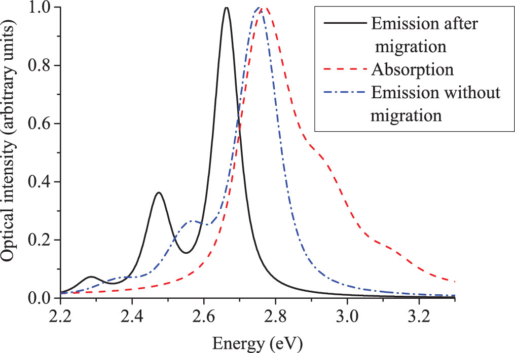
Figure 15: The calculated optical spectra of PPV assuming a statistical model of random polymer conformations. Exciton migration prior to emission causes a red-shift in energy, a narrowing of the inhomogeneous broadening, and a decrease in $I_{00}/I_{01}$. Reproduced from J. Chem. Phys. 141, 164103 (2014) with the permission of AIP publishing.

Some of the key features of exciton relaxation and dynamics described in this review are nicely encapsulated by Fig. 15. This figure shows the simulated absorption to all absorbing states, the fluorescence via emission from all LEGSs (which occurs in the absence of exciton migration), and the time-integrated fluorescence following exciton migration and emission from ‘trap’ chromophores. We observe that:

• The absorption spectrum and the emission spectrum assuming no exciton migration are broadly a mirror image. However, the absorption is broader and has a high energy tail as absorption occurs to both LEGSs and QEESs (as also shown in Fig. 3(b)), whereas, from Kasha’s law, emission occurs only from LEGSs following interconversion from QEESs.

• The emission following exciton migration is red-shifted, because the emissive states are in the low-energy tail of the density of states (as shown in Fig. 14).

• The inhomogeneous broadening of the post-migration emission is narrowed, because the emissive states have a narrower density of states than LEGSs.

• Similarly the intensity ratio, $I_{00}/I_{01}$, decreases, because on average emissive chromophores have shorter conjugation lengths than LEGSs.

VII Summary and Concluding Remarks

We have reviewed the various exciton dynamical processes in conjugated polymers. In summary, they are:

• Following photoexcitation, the initial dynamical process is the correlation of the exciton and phonons associated with high-frequency C-C bond vibrations. This quantum mechanical entanglement causes exciton-site decoherence, which is manifest as sub-10 fs fluorescence depolarization (see Section IV.1).

• Next, the energy that is transferred from the exciton to the nuclei is dissipated into the environment on a timescale determined by the strength of the system-bath interactions. For a hot exciton (i.e., a QEES) the system-bath interactions cause the entangled exciton-nuclear wavefunction to stochastically ‘collapse’ into a particular LEGS, causing the exciton density to be localized on a ‘chromophore’ (see Section IV.2).

• The fate of an exciton on a chromophore is now strongly dependent on the polymer chemical structure and the type of environment. For underdamped, freely rotating monomers, the coupling of the exciton to the low-frequency torsional modes creates an exciton-polaron, with associated planarization and exciton-density localization (see Section IV.3).

• For a polymer in solution, stochastic torsional fluctuations also causes the exciton-polaron to diffuse along the polymer chain; a process known as environment-assisted quantum transportRebentrost et al. (2009). The diffusion coefficient is linearly proportional to temperature (see Section V).

• For a polymer in the condensed phase, the dominant post-ps process is Förster resonant energy transfer and exciton diffusion. An exciton diffusing in the random energy landscape soon gets trapped in chromophores occupying the low-energy tail of the LEGSs density of states, exhibiting $\log t$ spectral diffusion. An exciton typically diffuses $\sim 10$ nm before radiative decay, with the diffusion length weakly increasing with decreasing disorder (see Section VI).

In this review we have argued that theoretical modeling of exciton dynamics over multiple time and length scales is only realistically possible by employing suitably parametrized coarse-grained exciton-phonon models. Moreover, to correctly account for the ultrafast processes of exciton-site decoherence and the relaxation of hot excitons onto chromophores, the exciton and vibrational modes must be treated on the same quantum mechanical basis and importantly the Ehrenfest approximation must be abandoned. We have also repeatedly noted that spatial and temporal disorder play a key role in exciton spectroscopy and dynamics; and it is for this reason that exciton dynamics is conjugated polymers is essentially an incoherent process.

In a previous reviewBarford and Marcus (2017) we explained how spectroscopic signatures are highly-dependent on polymer multiscale structures, and how - in principle - good theoretical modeling of excitons and spectroscopy can be used as a tool to predict these polymer structures. This review builds on that prospectus by describing how time-resolved spectroscopy can be understood via a theoretical description of exciton dynamics coupled to information on polymer multiscale structures. Again, the reverse proposition follows: time-resolved spectroscopy coupled to a theoretical description of exciton dynamics can be used to provide insights into polymer multiscale structures.