Understanding population annealing Monte Carlo simulations

Abstract

Population annealing is a recent addition to the arsenal of the practitioner in computer simulations in statistical physics and beyond that is found to deal well with systems with complex free-energy landscapes. Above all else, it promises to deliver unrivaled parallel scaling qualities, being suitable for parallel machines of the biggest calibre. Here we study population annealing using as the main example the two-dimensional Ising model which allows for particularly clean comparisons due to the available exact results and the wealth of published simulational studies employing other approaches. We analyze in depth the accuracy and precision of the method, highlighting its relation to older techniques such as simulated annealing and thermodynamic integration. We introduce intrinsic approaches for the analysis of statistical and systematic errors, and provide a detailed picture of the dependence of such errors on the simulation parameters. The results are benchmarked against canonical and parallel tempering simulations.

I Introduction

Over the last 70 years or so, computer simulations have undoubtedly developed into what can be considered a third pillar in science, complementing the classic duality of experiment and analytical theory Gramelsberger (2011). While this would not have been possible without the enormous increase of computational power available (spanning at least seven orders of magnitude), the invention of new and the improvement of existing algorithms for many problems has made a contribution of similar significance. The recent acceleration of the move towards higher and higher degrees of parallelism in computational architectures has added a new twist to this challenge: invent powerful algorithms that also have the potential to parallelize well over thousands or even millions of cores.

The hardest computational problems relate to systems with complex free-energy landscapes, often featuring phase transitions, entropic barriers and slow relaxation Janke (2007). To cope with such systems, that cover a broad range of areas from (spin) glasses through biopolymers to constraint optimization problems, simulators require methods that ensure a wide exploration of phase space, overcome energetic and entropic barriers, and artificially speed up slow dynamics. In Monte Carlo simulations, besides methods relating to the set of moves employed, that are typically highly tailored to the specific systems at hand such as in cluster updates for spin systems Swendsen and Wang (1987); Wolff (1989), the most important approaches are meta-algorithms that simulate a problem in a generalized ensemble. The most well-known schemes of this type are multicanonical simulations Berg and Neuhaus (1992), simulated and parallel tempering Geyer (1991); Hukushima and Nemoto (1996), and Wang-Landau sampling Wang and Landau (2001).

A more recent addition to this simulational toolbox are population annealing Monte Carlo simulations, where an ensemble of system copies is propagated in parallel while undergoing a gradual cooling process accompanied by periodic resampling steps Iba (2001); Hukushima and Iba (2003); Machta (2010). While this technique has only received significant attention in recent years Wang et al. (2015a, b); Barash et al. (2017a, b); Callaham and Machta (2017); Barash et al. (2019); Amey and Machta (2018); Barzegar et al. (2018); Christiansen et al. (2019); Rose and Machta (2019); Perera et al. (2020), related approaches have been known and used as particle filters in statistics Doucet and Johansen (2011) and as diffusion methods in quantum Monte Carlo von der Linden (1992). Also, there are closely related algorithms such as replication techniques Garel and Orland (1990) and the pruned-enriched Rosenbluth method (PERM) Grassberger (1997) for walks and polymers, or the nested sampling method for determining the density of states Pártay et al. (2014). In contrast to the more widely used Markov chain Monte Carlo (MCMC) methods, these approaches are based on the sequential sampling paradigm Doucet et al. (2001). While originating in Monte Carlo, it was recently demonstrated that it is indeed possible to generalize the scheme to molecular dynamics simulations Christiansen et al. (2019), and further generalization are likely to be found in the future.

Due to the employment of a population of system copies, the method is ideally suited for highly parallelized implementations, and excellent scaling results have been reported in applications Barash et al. (2017a); Barzegar et al. (2018); Weigel (2018); Christiansen et al. (2019); Russkov et al. (2021). The method hence bears great potential for attacking hard simulational problems, and indeed significant successes have been reported for problems such as spin glasses Wang et al. (2015b); Perera et al. (2020); Barash et al. (2019), hard disks Amey and Machta (2018) and biopolymers Christiansen et al. (2019). The theoretical understanding of the approach, however, is still in its infancy. While population annealing formally is a sequential Monte Carlo method Doucet et al. (2001), it requires as a crucial ingredient a way of additionally randomizing configurations through embedded single-replica Monte Carlo steps. This element is conveniently chosen to be a MCMC method, bearing the additional advantage of further driving the population towards equilibrium. As a consequence of this hybrid composition of the approach, its performance hence depends on the subtle interplay of correlations introduced into the population through resampling and the decorrelating effect of the MCMC moves. It is the purpose of the present paper to illustrate the implementation and properties of the method for a simple reference system, to provide a clear picture of how the statistical and systematic errors depend on the parameters of the method, and to provide techniques for monitoring the convergence of the simulation and analyzing the resulting data. The above mentioned success reports for non-trivial problems notwithstanding, the method has previously not been used for a non-trivial but well controlled model system (but see Ref. Machta and Ellis (2011) for a simple two-well problem). We fill this gap here by providing an in-depth study of population annealing applied to the fruit fly of statistical physics, the two-dimensional Ising model.

The rest of the paper is organized as follows. In Secs. II–IV we formally introduce the population annealing algorithm, followed by a short illustration of potential issues in applying it to the Ising model. Section V is devoted to an exploration of correlations introduced into the population through resampling. We show how these can be quantified through a blocking analysis on the tree-ordered population, leading to the introduction of the effective population size $R_{\mathrm{eff}}$, and how this approach can be used to estimate statistical errors from a single run. The dependence of statistical errors on the simulation parameters is further explored in Sec. VI. In Sec. VII we introduce the free-energy estimator and illustrate its relation to thermodynamic integration, as well as discussing the relevance and choice of weights for averaging over independent runs. Section VIII is devoted to a detailed analysis of the systematic errors of the method and their dependence on the simulation parameters. Finally, in Sec. IX we survey the performance of the approach and compare it to some more standard methods before presenting our conclusions in Sec. X.

II Algorithm

As outlined above, the approach is a hybrid of sequential algorithm and MCMC that simulates a population of configurations at each time, updating them with an embedded MCMC step and resampling the population periodically as the temperature is gradually lowered. Population annealing (PA) can hence be summarized as follows:

1. Set up an equilibrium ensemble of $R_{0}=R$ independent copies (replicas) of the system at inverse temperature $\beta_{0}$. Typically $\beta_{0}=0$, where this can be easily achieved.

2. Change the inverse temperature from $\beta_{i-1}$ to $\beta_{i}>\beta_{i-1}$. To maintain uniform weights, resample configurations $j=1,\ldots,R_{i-1}$ with their relative Boltzmann weight $\tau_{i}(E_{j})=\exp[-(\beta_{i}-\beta_{i-1})E_{j}]/Q_{i}$, where

   $$Q_{i}\equiv Q(\beta_{i-1},\beta_{i})=\frac{1}{R_{i-1}}\sum_{j=1}^{R_{i-1}}\exp[-(\beta_{i}-\beta_{i-1})E_{j}],$$ (1)

   resulting in a new population of size $R_{i}$.

3. Update each replica by $\theta$ rounds of an MCMC algorithm at inverse temperature $\beta_{i}$.

4. Calculate estimates for observable quantities ${\cal O}$ as population averages $\sum_{j=1}^{R_{i}}{\cal O}_{j}/R_{i}$.

5. Goto step 2 unless the target temperature $\beta_{\mathrm{f}}$ has been reached.

If we choose $\beta_{0}=0$, equilibrium configurations for the replicas can be generated by simple sampling, i.e., by assigning independent, purely random configurations to each copy. For systems without hard constraints such as typical spin models, this process can be implemented straightforwardly. For constrained systems such as polymers, one might need to revert to an MCMC simulation at a sufficiently high temperature instead.

To understand the origin of the resampling factors, it is useful to consider a more general algorithm, where resampling occurs less frequently or it is completely omitted. It is then necessary to keep track of the weight of each replica in the annealing process Iba (2001); Doucet and Johansen (2011). On changing the temperature from $\beta_{i-1}$ to $\beta_{i}$ the Boltzmann weight $W_{i-1}^{j}$ of a replica at energy $E_{j}$ is multiplied by the incremental importance weight $\gamma_{i}^{j}$ to arrive at the new weight $W_{i}^{j}$ at inverse temperature $\beta_{i}$,

$$W_{i}^{j}=W_{i-1}^{j}\gamma_{i}^{j},\;\;\;\gamma_{i}^{j}=\frac{Z_{\beta_{i-1}}}{Z_{\beta_{i}}}e^{-(\beta_{i}-\beta_{i-1})E_{j}^{i-1}},$$ (2)

where $Z_{\beta_{i}}$ is the canonical partition function. Note that at each temperature step it is the current energy $E_{j}^{i-1}$ of replica $j$ before resampling that enters here, hence the additional superscript $i-1$. The initial configurations are drawn from the uniform distribution, $W_{0}=1/Z_{0}$. If no MCMC steps according to step 3 would be performed such that $E_{j}^{i}=E_{j}^{0}$ for all $i$, this would correspond to simple sampling and the total weight would yield the canonical probability distribution, i.e, $W_{i}^{j}=Z_{\beta_{i}}^{-1}\exp(-\beta_{i}E_{j})$. In any case, if resampling occurs according to the prescription outlined in step 2 of the above algorithm, the average number of copies created for each replica equals $\tau_{i}(E_{j})$. To keep the overall distribution invariant, the weight of each surviving copy needs to be reduced by a factor $1/\tau_{i}(E_{j})$, resulting in a modified weight of

$$\begin{split}\widetilde{W}_{i}^{j}&=\widetilde{W}_{i-1}^{j}\frac{\gamma_{i}^{j}}{\tau_{i}(E_{j})}=\widetilde{W}_{i-1}^{j}\frac{Z_{\beta_{i-1}}}{Z_{\beta_{i}}}Q_{i}\\ &=W_{0}^{j}\frac{Z_{0}}{Z_{\beta_{1}}}\cdots\frac{Z_{\beta_{i-1}}}{Z_{\beta_{i}}}\prod_{k=1}^{i}Q_{k}=\frac{1}{Z_{\beta{i}}}\prod_{k=1}^{i}Q_{k}.\end{split}$$ (3)

These weights are now independent of the replica number $j$, such that estimates of observables follow from plain averages over the population as indicated in step 4. The product of factors $Q_{k}$, however, depends on the particular realization of PA run. As we discuss in Sec. VII.2 this has some consequences for combining results from different runs.

The resampling process in step 2 can be implemented in different ways Hukushima and Iba (2003); Machta (2010). As described in Ref. Hukushima and Iba (2003), in the process of resampling a total of $R_{i-1}$ replicas are chosen according to the probabilities $\tau_{i}(E_{j})/R_{i-1}$ using a multinomial distribution. As $R_{i}=R_{i-1}=R$, this amounts to a simulation at a fixed population size that might be particularly useful for an implementation of the algorithm on a distributed machine. Alternatively, one could use other resampling schemes with a fixed population size with a similar effect Gessert et al. . On the other hand, following Ref. Machta (2010) it is also possible to use a sum of Poisson distributions, leading to a fluctuating population size. To keep the fluctuations of the population size small in this case, it is useful to define the rescaled probabilities

$$\hat{\tau}_{i}(E_{j})=(R/R_{i-1})\tau_{i}(E_{j})$$ (4)

and draw the number of copies to make of replica $j$ according to a Poisson distribution of mean $\hat{\tau}_{i}(E_{j})$. Sampling from a multinomial or Poisson distribution using uniform (pseudo) random numbers efficiently is not completely straightforward Gentle (2003), so a useful and particularly simple alternative is to draw a random number $r$ uniformly in $[0,1)$ and take the number of copies of replica $j$ in the new population to be

$$r_{i}^{j}=\left\{\begin{array}[]{ll}\lfloor\hat{\tau}_{i}(E_{j})\rfloor&\mathrm{if}\;\;r>\hat{\tau}_{i}(E_{j})-\lfloor\hat{\tau}_{i}(E_{j})\rfloor\\ \lfloor\hat{\tau}_{i}(E_{j})\rfloor+1&\mathrm{otherwise}\end{array}\right..$$ (5)

Here, $\lfloor x\rfloor$ denotes the largest integer that is less than or equal to $x$ (i.e., rounding down). The new population size is $R_{i}=\sum_{j=1}^{R_{i-1}}r_{i}^{j}$. This method requires only a single call to the random number generator for each replica in the current population and no lookup tables, and additionally leads to very small fluctuations in the total population size. In general, it is possible to use an arbitrary distribution ${\cal P}(r_{i}^{1},\ldots,r_{i}^{R_{i-1}})$ as long as $\langle r_{i}^{j}\rangle=\hat{\tau}_{i}(E_{j})$, but the comparison of resampling methods is outside of the scope of the present work Li et al. (2020); Gessert et al. . Note that it is common that $r_{i}^{j}=0$ for some replicas, in which case these copies disappear from the population, while other configurations will be replicated several times.

In the standard setup, steps of equal size in inverse temperature are taken, i.e.,

$$\beta_{i}=\beta_{i-1}+\Delta\beta,$$ (6)

and $\Delta\beta$ is an adjustable parameter. It is also possible to make the temperature steps self-adaptive Barash et al. (2017a), but we do not discuss this possibility in the present paper that is focused on an analysis of the plain vanilla algorithm in the (possibly) simplest non-trivial system. Regarding the MCMC updates in step 3, we focus here on single-spin flip Metropolis and heatbath updates, i.e., local moves. The algorithm is completely general, however, and a combination with other techniques such as non-local cluster updates is straightforward Barzegar et al. (2018). Some possible effects of the choice of spin-update algorithm are discussed below in Sec. IV.2.

To allow for a fair comparison between PA and standard approaches, we usually consider simulations of the same overall run-time. As will be shown below in Sec. IX, the time overhead for resampling is quite negligible in most situations, almost all simulation time is spent flipping spins. For each population member, $\theta$ calls to the MCMC subroutine are performed after each resampling step. In the most general case, during these updates $\mu$ measurements are taken at equidistant time steps, followed by a temperature step $\beta\to\beta^{\prime}=\beta+\Delta\beta$. As a result, at each temperature step a sample of size $N=\mu R$ is available for all quantities considered. For the sake of simplicity and because we want to analyze the behavior of the algorithm as initially proposed, in the present work we focus on $\mu=1$, but we point out that choosing $\mu>1$ will in general improve the results Rose and Machta (2019).

III Model and observables

While many of the considerations developed below are fairly general, the numerical work is focused on the case of the two-dimensional ferromagnetic Ising model in zero field with Hamiltonian

$${\cal H}=-J\sum_{\langle i,j\rangle}s_{i}s_{j},$$ (7)

where interactions are only considered between nearest neighbors $\langle i,j\rangle$ on an $L\times L$ square lattice, and periodic boundary conditions are applied throughout. In the following we set $J=1$ to fix units. As is well known, this model undergoes a continuous phase transition at the inverse temperature $\beta_{c}=\frac{1}{2}\ln(1+\sqrt{2})$ McCoy and Wu (1973). In addition to the closed-form solution of the model first derived by Onsager Onsager (1944), many results are available also for finite systems Kaufman (1949); Ferdinand and Fisher (1969); Beale (1996), such that we can compare our simulation results to exact data.

For the simulations discussed here, at each temperature step we recorded the configurational energy $E_{k}$ and the magnetization $M_{k}$, $k=1,\ldots,N$ . From these we calculate the average energy per spin,

$$e=\frac{1}{L^{d}N}\sum_{k=1}^{N}E_{k},$$ (8)

where $d=2$ for the present case, the specific heat per spin,

$$C_{V}=\beta^{2}L^{d}\left(\frac{1}{L^{2d}N}\sum_{k=1}^{N}E_{k}^{2}-e^{2}\right),$$ (9)

as well as the (modulus of the) magnetization per spin,

$$m=\frac{1}{L^{d}N}\sum_{k=1}^{N}|M_{k}|,$$ (10)

and the magnetic susceptibility per spin,

$$\chi=\beta L^{d}\left(\frac{1}{L^{2d}N}\sum_{k=1}^{N}M_{k}^{2}-m^{2}\right).$$ (11)

It is of course easily possible to add other observables such as correlation lengths, overlaps, or correlation functions, but these will not be discussed explicitly here.

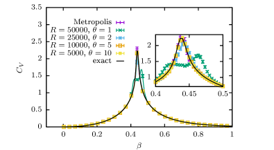
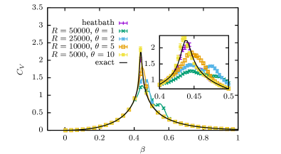
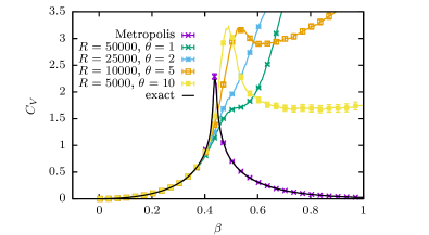
Figure 1: Top: Specific heat as estimated from population annealing with Metropolis update and fixed temperature steps $\Delta\beta=1/300$ for $L=64$. The pure Metropolis simulation shown for comparison uses $R=1$ with a total of $50\,000$ sweeps and measurements. The exact reference data are calculated according to Ref. Kaufman (1949); Ferdinand and Fisher (1969). Middle: Same as top panel, but for the heatbath update. Bottom: Results of PA simulations with the same parameters as in the top panel, but with the resampling step turned off. To make the comparison as fair as possible, in contrast to the rest of the paper all runs shown here use $\mu=\theta$ measurements per temperature step. The insets in the top and middle panels show detail around the peak close to the critical point of the system.

IV Initial assessment

IV.1 Equilibration

All comparisons in this section are for simulations of approximately the same overall run-time. That is, if $R$ is the population size, $\theta$ is the number of equilibration steps, and $N_{T}$ is the number of simulation temperatures, respectively, we keep the product $R\theta N_{T}$ constant. Also, the total number of measurements (samples in averages) is the same for each data set.

As is seen in the top panel of Fig. 1, a small number $\theta$ of equilibration steps is not sufficient to keep the population in equilibrium, at least in the critical region. On the other hand, it is clear that the resampling itself also has an equilibrating effect, as the deviations are much larger for identical runs with the resampling step switched off, cf. the bottom panel of Fig. 1.

From these initial experiments it becomes clear that a more systematic understanding of the behavior of the algorithm is required. In particular, we want to analyze the dependence of the quality of estimation on the parameters of the approach. In the following, we will present a principled study of the statistical and systematic error (bias) as a function of the main control parameters, the population size $R$, the size $\Delta\beta$ of the inverse temperature step, and the number $\theta$ of calls to the MCMC subroutine.

IV.2 Spin updates

The efficiency of the MCMC step clearly depends on the spin update employed. This is also visible comparing the top to the middle panel of Fig. 1, where the latter shows the specific heat for the discussed simulations, but using the heatbath update. For the Ising model studied here, single-spin flip updates essentially come in the Metropolis and heatbath variants (the Glauber update is equivalent to heatbath for Ising spins see, e.g., Ref. Janke (2008a)). Alternatively, one could also employ cluster updates which would clearly lead to vastly improved decorrelation in the critical region, but an investigation of these updates embedded in the population annealing heuristic is postponed to a later study.

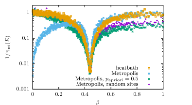
Figure 2: Inverse of the integrated autocorrelation time $\tau_{\mathrm{int}}(E)$ of the energy estimated from simulations of a $L=128$ system with a single replica and different spin updates.

Figure 2 shows the (inverse) integrated autocorrelation times of the internal energy for different variants of Metropolis updates as compared to the heatbath algorithm. For most temperatures, the sequential Metropolis update is found to lead to the smallest values of $\tau_{\mathrm{int}}(E)$. It is well known that Metropolis updates are more efficient than heatbath for Ising spins (in contrast to systems with more micro-states such as the $q$-state Potts model with $q>2$, see Ref. Loison et al. (2004)). This effect is well visible in Fig. 2, especially in the critical region. Also, sequential updating, while (or because) it violates detailed balance and only fulfills the necessary condition of balance, in general leads to faster decorrelation Berg (2004); Ren and Orkoulas (2006). Initially surprisingly, however, the sequential Metropolis update does not work well at high temperatures. As is easily seen, the Metropolis acceptance probability $\min[1,\exp(-\beta\Delta E)]\to 1$ as $\beta\to 0$, hence virtually all proposed spin flips are accepted for very small $\beta$. In a sequential scheme, however, this means that the full spin configuration is being almost perfectly inverted through each sweep, which clearly does not lead to a proper decorrelation of configurations. In other words, the sequential Metropolis update is not ergodic in the limit $\beta\to 0$. A number of modifications can be applied to amend this, for instance the introduction of an a priori flipping probablity less than one in the sequential update or a reversion to the random-order update. As can be seen from Fig. 2, these recitify the problem of non-ergodicity for $\beta\to 0$, but at the expense of somewhat increased autocorrelation times for all the other temperatures. In practice, the non-ergodicity of the sequential Metropolis update does not cause any major problems in PA simulations unless one is interested in results at very small $\beta$, and we have hence used this update for a range of the simulations reported here. The effects of deviations for the smallest $\beta$ can be seen in some of the figures, for instance Figs. 5 and 10.

V Correlations

V.1 Families

It is clear that the quality of approximation and, in particular, the statistical errors will crucially depend on the level of correlations built up through resampling in the population. A conservative way of estimating these effects is based on the study of families Wang et al. (2015c, a), i.e., the descendants of a single configuration in the initial population. If the simulation is started with configurations created by simple sampling at $\beta=0$, these are rigorously independent of each other. (This is only approximately the case for systems with constraints where the initial configurations might be generated by sampling them from a single simulation at high temperatures Christiansen et al. (2019).) To assess statistical errors in a PA simulation, we would like to estimate the variance of the mean

$$\overline{\cal O}=\frac{1}{R}\sum_{j=1}^{R}{\cal O}_{j}$$ (12)

of an observable ${\cal O}$. Following arguments proposed in Ref. Wang et al. (2015a), we first consider the case that ${\cal O}$ takes the same value for all replicas of each family, corresponding to the limit $\theta=0$. Denote the fraction of the present population that descends from an initial replica $k$ as $\mathfrak{n}_{k}$. Then,

$$\overline{\cal O}=\sum_{k=1}^{f}\mathfrak{n}_{k}{\cal O}_{k},$$ (13)

where $\mathcal{O}_{k}$ denotes the value of the observable ${\cal O}$ in the $k$-th family (at the current temperature), and $f$ is the number of surviving families at the current step. To estimate the variance $\sigma^{2}(\overline{\cal O})$, we further assume that $\sigma^{2}({\cal O}_{k})=\sigma^{2}({\cal O})$, implying that the variance is not correlated with the family size. Since the families are uncorrelated, the individual variances add up and one finds

$$\sigma^{2}(\overline{\cal O})=\sigma^{2}({\cal O})\sum_{k}\mathfrak{n}_{k}^{2}.$$ (14)

In the fully uncorrelated case where each family has only one member, one has $\mathfrak{n}_{k}=1/R$ and hence

$$\sigma^{2}(\overline{\cal O})=\frac{\sigma^{2}({\cal O})}{R},$$ (15)

as expected for the variance of the mean of uncorrelated random variables. More generally, we might consider the quantity $R_{t}=R/\rho_{t}$ with

$$\rho_{t}=R\sum_{k}{\mathfrak{n}}_{k}^{2}$$ (16)

an effective number of uncorrelated replicas in the $\theta=0$ limit . $\rho_{t}$ represents the mean square family size Wang et al. (2015a).

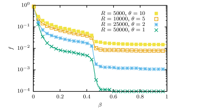
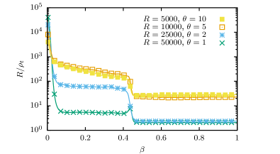
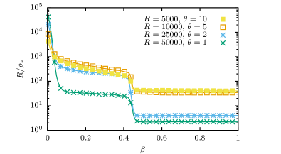
Figure 3: Effective number of independent replicas as estimated from the family statistics for PA simulations with $L=64$ (Metropolis update, $\Delta\beta=1/300$). Top: number $f$ of surviving families. Middle: $R/\rho_{t}$ according to Eq. (16). Bottom: $R/\rho_{s}$ according to Eq. (18).

Alternatively, it was also proposed in Ref. Wang et al. (2015a) to consider the entropy of the family size distribution,

$$S_{f}=-\sum_{k}\mathfrak{n}_{k}\ln\mathfrak{n}_{k},$$ (17)

such that $R_{s}=R/\rho_{s}$ with

$$\rho_{s}=R/\exp(S_{f})$$ (18)

can be considered as an alternative measure of the effective number of independent measurements. Figure 3 summarizes the behavior of these family-related correlation measures for runs of the 2D Ising model. It is clear that they are quite similar to each other, showing a general decline through the loss of diversity from resampling. It can be shown that at the early stages of the process the decay in family numbers is exponential, as in each step a fraction of $1-\kappa_{i}$ is lost, where $\kappa_{i}$ is the overlap of the energy histograms (i.e., the probability distribution of energies) at temperature steps $i$ and $i+1$. At intermediate stages, however, the decay levels off as families consist of more than one member and so the probability of their extinction is decreased. In the vicinity of the critical point there is a further steep decline in all three quantities. This effect has two causes, namely (1) due to the overlap of energy histograms at neighboring temperatures having a minimum close to $\beta_{c}$, there is a stronger multiplication of replicas in the low-energy wing of the distribution leading to a stronger correlation in surviving families, and (2) at least for small $\theta$ the population members are not fully relaxed at a given temperature, leading to a further reduction of the overlap of the actual histogram at the higher temperature and the equilibrium histogram at the lower one.

V.2 Effective population size

These measures related to the family statistics, however, neglect the effect of the spin flips which, as is seen in Fig. 1 are of crucial importance for the effectiveness of the full algorithm (in order to get correct results from resampling alone exponentially large population sizes would be required). We expect, for instance, that at low temperatures $\beta\gg\beta_{c}$ the local dynamics will have no problem at equilibrating the population (although, formally, the typical single spin-flip dynamics are not rapidly mixing as there remains a barrier between the pure phases, but this is not seen in the behavior of energetic quantities). Hence, it is clearly not the case that the “diversity” in the population is minimal at the lowest temperature, but we rather expect it to become minimal in the vicinity of the critical point and then to come up again due to the spin-flip updates.

This behavior is captured in correlations between different members of the population, which are the property we are actually trying to measure when considering the family statistics. This is analogous to temporal correlations in standard MCMC simulations which can be analyzed with a well-known toolbox of techniques weigel:09 ; Sokal (1997). Consider an observable ${\cal O}$. In an uncorrelated sample, we know that the variance of the mean $\overline{\cal O}$ is inversely linear in the sample size $R$ Feller (1968),

$$\sigma^{2}(\overline{{\cal O}})=\frac{\sigma^{2}({\cal O})}{R}.$$ (19)

In reality, however, there are correlations introduced through the resampling process (but reduced by the effect of the MCMC subroutine), such that the variance of the mean decays only with an effective number of samples $R_{\mathrm{eff}}({\cal O})\leq R$, i.e.,

$$\sigma^{2}(\overline{{\cal O}})=\frac{\sigma^{2}({\cal O})}{R_{\mathrm{eff}}}=\frac{\sigma^{2}({\cal O})}{R/2\tau_{R}^{\mathrm{int}}},$$ (20)

where $\tau_{R}^{\mathrm{int}}=\tau_{R}^{\mathrm{int}}({\cal O})$ measures the degree of correlation in replica space. Assuming that we can estimate $\sigma^{2}(\overline{{\cal O}})$ and $\sigma^{2}({\cal O})$, this provides an estimate of the effective number of independent measurements ,

$$R_{\mathrm{eff}}({\cal O})=\frac{\sigma^{2}({\cal O})}{\sigma^{2}(\overline{{\cal O}})}.$$ (21)

In general, the variance of the mean is given by

$$\sigma^{2}(\overline{{\cal O}})=\frac{1}{R^{2}}\sum_{i,j=1}^{R}\left(\langle{\cal O}_{i}{\cal O}_{j}\rangle-\langle{\cal O}_{i}\rangle\langle{\cal O}_{j}\rangle\right)=\frac{1}{R^{2}}\sum_{i,j=1}^{R}\Gamma_{ij},$$ (22)

where $\Gamma_{ij}$ is the covariance matrix of the measurements ${\cal O}_{i}$, $i=1,\ldots,R$. Members of the population are more strongly correlated the more recently in terms of previous temperature steps they have originated from the same common ancestor. We can localize these correlations by deliberately always putting offspring of the same parent configuration next to each other in the resampled population. We then expect the correlations to be local, i.e., $\lim_{|i-j|\to\infty}\Gamma_{ij}=0$ sufficiently fast, such that the variance of the mean can be determined by considering the statistics of a blocked series of $n$ bins with averages Flyvbjerg and Petersen (1989)

$${\cal O}_{i}^{\mathrm{B}}=\frac{1}{B}\sum_{j=(i-1)B+1}^{iB}{\cal O}_{j},\;\;\;\;i=1,\ldots,n,$$ (23)

where $B=R/n$ is the number of elements per block (for simplicity, we assume that $n$ is chosen to divide $R$). If blocks are large enough, they will be effectively uncorrelated and we can use the naive (uncorrelated) variance estimator to find the variance of the mean,

$$\hat{\sigma}^{2}(\overline{{\cal O}})=\frac{1}{n(n-1)}\sum_{i=1}^{n}({\cal O}^{\mathrm{B}}_{i}-\overline{{\cal O}^{\mathrm{B}}})^{2}.$$ (24)

Alternatively, in particular to reduce bias for non-linear functions of observables, one might want to use an analysis based on jackknife blocks, where all data apart from the $i$-th block of Eq. (23) are gathered in block $i$, i.e.,

$${\cal O}_{i}^{\mathrm{J}}=\frac{B}{R-B}\sum_{j\neq i}{\cal O}_{j}^{\mathrm{B}},\;\;\;\;i=1,\ldots,n.$$ (25)

The variance of the mean then follows from the corresponding jackknife estimator Efron and Tibshirani (1994),

$$\hat{\sigma}^{2}(\overline{{\cal O}})=\frac{n-1}{n}\sum_{i=1}^{n}({\cal O}^{\mathrm{J}}_{i}-\overline{{\cal O}^{\mathrm{J}}})^{2}.$$ (26)

The variance $\sigma^{2}({\cal O})$, on the other hand, can be estimated by the standard (uncorrelated) variance estimator on the unblocked series, where bias corrections are proportional to $\tau_{R}^{\mathrm{int}}/R$ and are hence not relevant in the desirable case where $R\gg\tau_{R}^{\mathrm{int}}$.

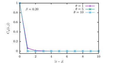
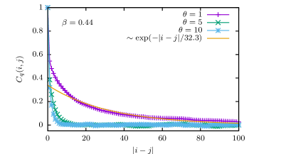
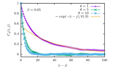
Figure 4: Distance dependence of the overlap correlation function $C_{q}(i,j)$ according to Eq. (27) for PA runs of a $L=16$ system with $R=50\,000$ and $\theta=1$, $5$, and $10$, respectively. Top: at high temperatures the population is nearly uncorrelated. Middle: close to criticality, significant correlations develop that asymptotically follow the form $C_{q}(i,j)\sim\exp(-|i-j|/\tau_{R})$ with $\tau_{R}=32.3$ ($\theta=1$), $\tau_{R}=3.0$ ($\theta=5$), and $\tau_{R}=1.8$ ($\theta=10$), respectively. Bottom: for the overlap, correlations persist in the ordered phase.

For the present problem, locality of correlations can be ensured through the resampling process by placing the $r_{i}^{j}$ copies of each member of the parent population according to Eq. (5) at adjacent indices of the resampled population. Hence at each stage members of the same families are grouped together. Correlations between population members then decay with the distance $|i-j|$ in index space since the larger this separation the further in the past of the resampling tree do the instances have a common ancestor, with the extreme case being that of members of different families that are by construction completely uncorrelated. To illustrate this, we consider the distance dependence of the configurational overlap between replicas, i.e.,

$$C_{q}(i,j)=\frac{1}{L^{d}}\sum_{k=1}^{L^{d}}s_{k}^{(i)}s_{k}^{(j)},$$ (27)

where $s_{k}^{(i)}$ denotes the $k$-th spin variables in replica $i$. We expect $C_{q}(i,j)$ to be translationally invariant in replica-index space, and so Fig. 4 illustrates the behavior of $C_{q}(|i-j|)$ at different temperatures for runs of $R=50\,000$ replicas. It is seen that there is a clear decay of $C_{q}(i,j)$ with the replica distance $|i-j|$, and it is compatible with an exponential asymptotic form,

$$C_{q}(i,j)\sim\exp(-|i-j|/\tau_{R}),$$ (28)

where $\tau_{R}$ is negligible for high temperatures. Close to criticality for $\beta=0.44$, the tail of $C_{q}(i,j)$ for $\theta=1$ is compatible with the form (28) with $\tau_{R}\approx 32.3$, while for $\theta=5$ it is reduced to $\tau_{R}\approx 3.0$, and for $\theta=10$ we find $\tau_{R}\approx 1.8$. At least for $\theta=1$ it is clearly seen that the initial decay does not follow the same single exponential. This is in line with the behavior of time series in MCMC, where the decay is in general understood to be a superposition of many exponentials Sokal (1997). One effect contributing to this behavior for the present case of correlations in the population of PA is that even for nearby replicas there is a chance of them belonging to different families, which are by definition completely uncorrelated. The decay of correlations in the regime of very small $|i-j|$ is therefore faster than the asymptotic decay, cf. the middle and lower panel of Fig. 4.

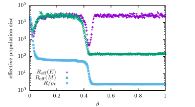
Figure 5: Effective number of statistically independent samples (for the energy measurement) in PA and standard canonical simulations for an $L=64$ system and different population sizes for the Metropolis (top panel) and heatbath updates (middle panel; for the legend of data sets see the upper panel). The bottom panel shows the effective population sizes $R_{\mathrm{eff}}(E)$ for the energy and $R_{\mathrm{eff}}(M)$ for the magnetization for $R=25\,000$, $\theta=2$ in comparison to the quantity $R/\rho_{t}$ based on family statistics alone, illustrating that the latter is a lower bound for the former, but it is far from being tight. All simulations shown use inverse temperature steps of size $\Delta\beta=1/300$.

Applying the blocking analysis to the thus ordered population allows one to determine an effective number of statistically independent replicas according to Eq. (21). The resulting values extracted from the variances of the energy estimates are shown in Fig. 5. Initially, for $\beta=0$, the population is uncorrelated and hence $R_{\mathrm{eff}}=R$. The resampling generates correlations, leading to a general decay of $R_{\mathrm{eff}}$. The spin flips, on the other hand, decorrelate replicas and therefore work towards increasing $R_{\mathrm{eff}}$. On approaching the critical point, spin flips become less and less effective, leading to a decay of $R_{\mathrm{eff}}$ there, similar to what is observed for the family-related observables $R/\rho_{t}$ and $R/\rho_{s}$ in Fig. 3. In contrast to the latter quantities that do not feel the effect of spin flips, however, $R_{\mathrm{eff}}(E)$ is able to recover to $R_{\mathrm{eff}}(E)=R$ deep in the ordered phase. As we shall see below, $R_{\mathrm{eff}}$ plays a central role in the characterization of the performance of a PA run. The bottom panel of Fig. 5 illustrates the fact that the family-related quantity $R/\rho_{t}$ is a lower bound for $R_{\mathrm{eff}}$, but it is far from tight and it can in fact be orders of magnitude below $R_{\mathrm{eff}}$. Due to the dynamic ergodicity breaking, $R_{\mathrm{eff}}(M)$ does not recover in the ordered phase in the way observed for $R_{\mathrm{eff}}(E)$. Note, however, that this is dependent on the update algorithm employed and, for instance, if using a cluster-update method Swendsen and Wang (1987); Wolff (1988, 1989) both $R_{\mathrm{eff}}(E)$ and $R_{\mathrm{eff}}(M)$ approach $R$ also in the ordered phase.

VI Statistical errors

Note that the same blocking analysis provides estimates of statistical errors of quantities sampled in PA from a single simulation run, such that the error estimates through multiple runs initially proposed in Ref. Machta (2010) are no longer necessary. To this end one can use the blocked estimator (24) or, equivalently, the jackknife estimator (26) for the variance of the mean. For non-linear observables such as the specific heat, correlation length etc. one should instead always use the jackknife form (26) in order to minimize the statistical bias in error estimates Efron and Tibshirani (1994); Janke (2002); Young (2015).

A useful check of self-consistency is to monitor the number of independent samples estimated through Eq. (21). The ratio $R/R_{\mathrm{eff}}$ is like an integrated autocorrelation time. It should be much smaller than the size $B=R/n$ of a block for the approach to be self-consistent. This is the case if

$$R_{\mathrm{eff}}\gg n.$$ (29)

Since we typically use $n=100$ to arrive at reliable error estimates, $R_{\mathrm{eff}}$ should not fall below a few thousand replicas to avoid bias in the error estimation. At the same time, however, the PA simulation itself is no longer reliable if this condition is not met as we do not have sufficient statistically independent information to sample the energy distribution faithfully. As we shall see below, $R_{\mathrm{eff}}$ also affects the simulation bias. Monitoring $R_{\mathrm{eff}}$ hence serves as an important indicator of the trustability of the simulation results – much like the integrated autocorrelation time provides such an indicator for MCMC simulations Sokal (1997).

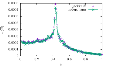
Figure 6: Estimated standard deviation of the mean (a.k.a. error bar) of the internal energy, $\sigma(\overline{E})$, for the $L=32$ Ising model as estimated from PA simulations with the blocking technique using Eq. (26) compared to the unbiased estimate resulting from repeating the full simulation 200 times with different sequences of random numbers ($R=50\,000$, $\theta=10$, $\Delta\beta=0.01$). All simulations use the Metropolis update.

To confirm the reliability of this way of estimating statistical errors, we show in Fig. 6 a comparison of the error bars thus computed to the errors estimated independently from repeating the PA simulation 200 times with independent seeds of the random-number generator. These simulations for $L=32$, $R=50\,000$ and $\theta=10$ show full compatibility between the two approaches. A more detailed analysis shown in Fig. 7 illustrates the dependence on population size (which shows no differences between the two approaches) and the number $\theta$ of rounds of spin flips. It is clear that as soon as the number $R_{\mathrm{eff}}$ of independent samples becomes too small, and hence the population too strongly correlated, the blocking analysis becomes unreliable (we find that $R_{\mathrm{eff}}\approx 600$ for $R=50\,000$ near criticality for $\theta=1$). As in the analysis of MCMC simulations, it is hence quite easily possible to monitor the self-consistency of the error analysis.

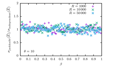
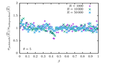
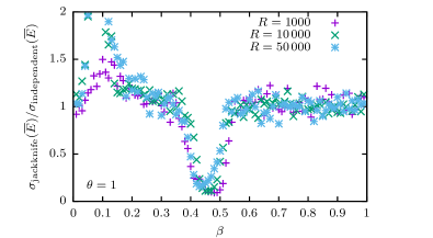
Figure 7: Ratio of error bars estimated from the jackknife analysis of a single PA run and from the fluctuation between 200 independent runs for PA simulations of the 2D Ising model with $L=32$ ($\Delta\beta=0.01$). Deviations from the target value 1.0 occur if the number $R_{\mathrm{eff}}$ of independent measurements becomes too small and hence the blocks in the analysis are no longer independent. In this case the blocking or jackknifing approach underestimates the errors (bottom panel).

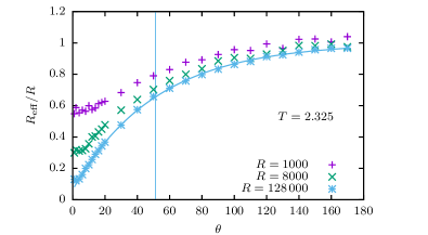
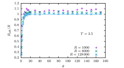
Figure 8: Effective relative number of independent members of the population, $R_{\mathrm{eff}}/R$, for PA simulations of the $L=64$ system with $\Delta\beta=0.005$ and varying population sizes in dependence of the $\theta$ values. Upper panel: runs at temperature $T=2.325$, close to the critical point. Lower panel: runs at $T=2.5$ in the disordered phase. The lines show fits of the functional form (30) to the data with $\tau_{\mathrm{eff}}=51.2$ (upper panel) and $\tau_{\mathrm{eff}}=2.2$ (lower panel), respectively.

It remains to discuss the dependence of statistical errors on the parameters $R$, $\Delta\beta$ and $\theta$ of the PA simulation. At each resampling step, correlations are introduced into the population through the creation of identical copies of some members and the elimination of others, leading to a reduction of the effective population size $R_{\mathrm{eff}}$. The subsequent application of spin flips onto each replica, on the other hand, works towards removing such correlations between population members with common ancestors. The quantitative effect of these processes is discussed in more detail in Appendix A. The corresponding correlation and decorrelation of replicas depends on the model as well as on temperature, such that the overall effect on $R_{\mathrm{eff}}$ after a number of temperature steps is hard to infer in closed form. Overall, however, one clearly expects an exponential dependence of $R_{\mathrm{eff}}$ on $\theta$, and we find the following relation to accurately describe the data,

$$R_{\mathrm{eff}}=R\left[1-c\exp(-\theta/\tau_{\mathrm{eff}})\right],$$ (30)

where $c$ is some constant that might depend on further simulation parameters such as $\Delta\beta$ (see below). To illustrate this, in Fig. 8 we show the behavior of $R_{\mathrm{eff}}/R$ as a function of $\theta$ for temperatures $T=2.325$ and $T=2.5$ and a range of different population sizes. As the population size is increased, $R_{\mathrm{eff}}$ approaches the form (30), which is very well observed for the largest population with $R=128\,000$ as is illustrated by the fit of the form (30) shown in the upper panel of Fig. 8 that yields $\tau_{\mathrm{eff}}\approx 51.2$. Given that we used $B=31$, $62$ and $250$ bins for $R=1000$, $8000$, and $128\,000$, respectively, our self-consistency condition $R_{\mathrm{eff}}\gg n$, which in practice we read as $R_{\mathrm{eff}}>50n$, implies that all estimates of $R_{\mathrm{eff}}$ for $R=1000$ are unreliable, while this applies only to $R_{\mathrm{eff}}/R\leq 0.4$ for $R=8000$ and $R_{\mathrm{eff}}/R\leq 0.09$ for $R=128\,000$, which appears to be in line with the observed deviations in the upper panel of Fig. 8 . As is apparent from the lower panel, such problems only occur for the smallest values of $\theta$ for the higher temperature $T=2.5$. There, the functional form (30) works well for all three population sizes, and a fit yields $\tau_{\mathrm{eff}}\approx 2.2$.

Regarding the dependence of statistical errors on the (inverse) temperature step $\Delta\beta$, it is clear that $R_{\mathrm{eff}}$ should approach $R$ as $\Delta\beta\to 0$ since there is no correlating effect from resampling for $\Delta\beta=0$ and the number of Monte Carlo sweeps performed in a given temperature interval increases inversely proportional to $\Delta\beta$. In Fig. 9 we show $1-R_{\mathrm{eff}}/R$ as a function of $\Delta\beta$ for different choices of $\theta$, and it is clear that the behavior is linear for small $\Delta\beta$. In fact, it is possible to derive this scaling for the behavior in a single temperature step from the arguments laid out in Appendix A. We hence generalize relation (30) to include the effect of varying temperature steps,

$$R_{\mathrm{eff}}=R\left[1-\frac{\Delta\beta}{\Delta\beta_{0}}\exp(-\theta/\tau_{\mathrm{eff}})\right],$$ (31)

which is correct in the limit $\Delta\beta\to 0$. Here, $\Delta\beta_{0}$ is an empirical constant, and from the fits shown in Fig. 9 we find $\Delta\beta_{0}\approx 0.005$, which is in line with the results of Fig.  8, where we found $c\approx 1$ for the step size $\Delta\beta=0.005$ used there.

The population size affects the statistical errors in the expected way. In well equilibrated simulations statistical errors decay as $1/\sqrt{R}$ which is an immediate consequence of the number of families growing linearly with $R$, such that the number of independent samples must also grow linearly with the population size. This fact is illustrated in the scaling plots for the error bars of the energy in Fig. 10. For $\theta=10$ the simulations are sufficiently close to equilibrium everywhere and clear $1/\sqrt{R}$ scaling of statistical errors is observed. For $\theta=1$, however, such behavior is almost nowhere observed: for very high temperatures this is prevented by the non-ergodicity of the sequential Metropolis update (cf. Sec. IV.2), and in the critical region it is prevented by critical slowing down. Only for very low temperatures a scaling collapse is observed.

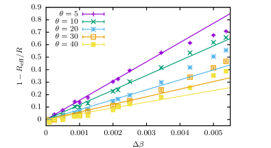
Figure 9: Relative deviation of the effective population size $R_{\mathrm{eff}}$ from the actual population size $R$ as a function of $\Delta\beta$ for an $L=64$ system close to criticality for a range of different values of $\theta$ ($\beta=0.43$, $R=10\,000$). The data are averaged over 200 independent runs. The lines show one-parameter fits of the form $1-R_{\mathrm{eff}}/R=A\Delta\beta$.

VII Free energies

VII.1 Free-energy estimate

As was already shown by Hukushima and Iba Hukushima and Iba (2003), population annealing naturally allows to estimate partition-function ratios or, equivalently, free-energy differences. This can be motivated by the following telescopic product expansion of the partition function,

$$\begin{split}-\beta_{i}F(\beta_{i})&=\ln Z_{\beta_{i}}=\ln\left(\frac{Z_{\beta_{i}}}{Z_{\beta_{i-1}}}\frac{Z_{\beta_{i}-1}}{Z_{\beta_{i-2}}}\cdots\frac{Z_{\beta_{1}}}{Z_{\beta_{0}}}Z_{\beta_{0}}\right)\\ &=\ln Z_{\beta_{0}}+\sum_{j=0}^{i-1}\ln\frac{Z_{\beta_{j+1}}}{Z_{\beta_{j}}}.\end{split}$$ (32)

The partition function ratios on the r.h.s. are equivalent to expectation values of ratios of Boltzmann factors, $\langle\exp[-(\beta_{k}-\beta_{k-1})E]\rangle_{\beta}=Z_{\beta_{k}}/Z_{\beta_{k-1}}$, which in turn are estimated in PA by the normalization factors $Q(\beta_{k-1},\beta_{k})$, cf. Eq. (1). As a consequence, a natural estimator of the free energy at inverse temperature $\beta_{i}$, $i=0,\ldots,N_{T}$ (there are $N_{T}+1$ temperatures including $\beta_{0}$) is given by Machta (2010)

$$-\beta_{i}\hat{F}_{i}=\ln Z_{\beta_{0}}+\sum_{k=1}^{i}\ln Q(\beta_{k-1},\beta_{k}).$$ (33)

If $\beta_{0}=0$ is chosen, $Z_{\beta_{0}}$ corresponds to the number of microstates, which usually can be worked out exactly. For the present case of Ising systems, we have $\ln Z_{\beta_{0}}=L^{d}\ln 2$.

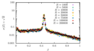
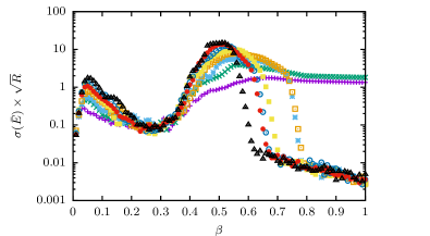
Figure 10: Estimated standard deviation of the mean times $\sqrt{R}$ for the energy of the $L=64$ Ising model for PA simulations with a range of different population sizes $R$ for $\theta=10$ (top) and $\theta=1$ (bottom), respectively ($\Delta\beta=0.01$).

While the form Eq. (33) might appear like an expression that is specific to the PA method, it is in fact a slight generalization of what is more traditionally known in the field of Monte Carlo simulations as thermodynamic integration. This is easily seen by noting that in the limit $\Delta\beta\to 0$ of small (inverse) temperature steps we have

$$\begin{split}-\beta_{i}F(\beta_{i})&=\ln Z_{0}+\ln\prod_{k=1}^{i}\langle e^{-(\beta_{k}-\beta_{k-1})E}\rangle_{\beta_{k-1}}\\ \stackrel{{\scriptstyle\Delta\beta_{k}\to 0}}{{\longrightarrow}}&\sum_{k}(-\Delta\beta_{k})\langle E\rangle_{\beta_{k-1}}+\ln Z_{o}\\ \stackrel{{\scriptstyle\Delta\beta_{k}\to 0}}{{\longrightarrow}}&\int_{\beta_{0}}^{\beta_{i}}\langle-E(\beta^{\prime})\rangle\,\mathrm{d}\beta^{\prime}+\ln Z_{0},\\ \end{split}$$ (34)

where $\Delta\beta_{k}=\beta_{k}-\beta_{k-1}$. Equation (34) is the standard expression for calculating free energies via thermodynamic integration Janke (2003); Landau and Binder (2015); Barash et al. (2017b). In fact, the above relation can be read in the opposite direction also, telling us that a more accurate version of thermodynamic integration that disposes of the requirement of taking small inverse temperature steps is given by the first line of Eq. (34). (Something which surely must have been observed somewhere else before.)

Apart from being an interesting observation, relation (34) provides a useful guideline allowing us to understand the behavior of PA in the limit of small temperature steps. In the above limit $\Delta\beta\to 0$ of thermodynamic integration, an alternative PA estimator of the free energy is given by

$$-\beta\tilde{F}(\beta)=\ln Z_{0}-\int_{\beta_{0}}^{\beta}\overline{E}(\beta^{\prime})\,\mathrm{d}\beta^{\prime},$$ (35)

where $\overline{E}(\beta_{i})=(1/R_{i})\sum_{j}E_{j}$ is the population average of the internal energy. As we shall see in Sec. VII.2 the variance of the free-energy estimate is of some relevance for the reliability of PA. According to Eq. (35) the variance of $\beta\tilde{F}$ is given by

$$\sigma^{2}(\beta\tilde{F})=\sigma^{2}\left[\int_{\beta_{0}}^{\beta}\overline{E}(\beta^{\prime})\,\mathrm{d}\beta^{\prime}\right].$$ (36)

If the populations at successive temperatures are statistically independent of each other, one can interchange the variance and the integral to find

$$\sigma^{2}(\beta\tilde{F})\approx\Delta\beta\int_{\beta_{0}}^{\beta}\sigma^{2}\left[\overline{E}(\beta^{\prime})\right]\,\mathrm{d}\beta^{\prime}.$$ (37)

Hence, the variance of the free energy estimator corresponds to the integral (sum) of the squared error bars of the energies along the trajectory in $\beta$. Clearly, the variance of $\beta\tilde{F}$ is proportional to the temperature step $\Delta\beta$ in this limit. As we shall see below in Sec. VIII.2, this implies that the bias of PA is also linear in $\Delta\beta$. If also the members of the population at a given temperature are uncorrelated to each other, one concludes that

$$\sigma^{2}(\beta\tilde{F})\approx\frac{\Delta\beta}{R}\int_{\beta_{0}}^{\beta}\sigma^{2}\left[E(\beta^{\prime})\right]\,\mathrm{d}\beta^{\prime}.$$ (38)

Finally, if the simulation is in equilibrium at all times, one can also write this as

$$\sigma^{2}(\beta\tilde{F})\approx\frac{\Delta\beta}{R}\int_{\beta_{0}}^{\beta}\frac{C_{V}(\beta^{\prime})L^{d}}{\beta^{\prime 2}}\,\mathrm{d}\beta^{\prime}.$$ (39)

The inversely linear dependence of the variance of the free-energy estimate on $R$ is expected, and a more general argument in support of this relation is discussed below in Sec. VIII.2. In the presence of correlations between population members, Eq. (38) becomes instead

$$\sigma^{2}(\beta\tilde{F})\approx\Delta\beta\int_{\beta_{0}}^{\beta}\frac{\sigma^{2}\left[E(\beta^{\prime})\right]}{R_{\mathrm{eff}}(\beta^{\prime})}\,\mathrm{d}\beta^{\prime}.$$ (40)

This relation shows the intimate relation of $\sigma^{2}(\beta\tilde{F})$ and the effective population size $R_{\mathrm{eff}}$. Effectively differentiating relation (35), we find for the free-energy contribution of one step in the limit $\beta\to 0$,

$$\beta\Delta\tilde{F}\approx\Delta\beta\overline{E}(\beta),$$ (41)

and hence

$$\begin{split}\sigma^{2}(\beta\Delta\tilde{F})&\approx(\Delta\beta)^{2}\sigma^{2}[\overline{E}(\beta)]\\ &=(\Delta\beta)^{2}\frac{\sigma^{2}(E)}{R_{\mathrm{eff}}}=(\Delta\beta)^{2}\frac{C_{V}L^{d}}{\beta^{2}R_{\mathrm{eff}}}.\end{split}$$ (42)

To illustrate the regime of validity of the thermodynamic integration approximation, we show in Fig. 11 the variance of the free-energy estimator (33) as estimated from the statistics over 200 independent runs in comparison to the approximations of Eqs. (39) and (40), respectively. For $\Delta\beta=0.01$ the approximations track the independent estimate quite well until reaching the critical regime, where significant deviations start to appear. It is clear, however, that the expression (40) involving $R_{\mathrm{eff}}$ is a more accurate description than the estimator (39). As the inverse temperature step is decreased to $\Delta\beta=0.0025$ and finally to $\Delta\beta=0.001$ the agreement with the independent estimate of $\sigma^{2}(\beta\hat{F})$ improves significantly.

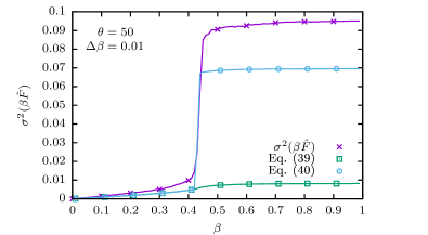
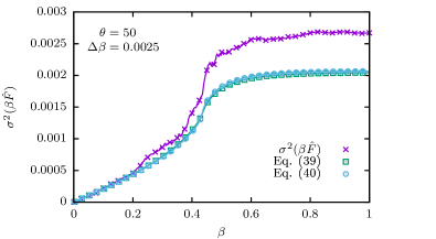
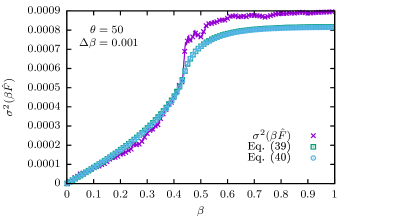
Figure 11: Variance of the free-energy estimator $\beta\hat{F}$ for different choices of the inverse temperature step $\Delta\beta$. The purple crosses show the variance of the quantity (33) as estimated from 200 independent PA runs. The green squares and blue circles show the estimates derived via Eqs. (39) and (40), respectively, from the same simulations ($L=64$, $R=10\,000$, $\theta=50$). For clarity of presentation, only every 10th temperature point is plotted with a symbol.

VII.2 Weighted averages

For technical reasons, it is not always possible to consider in a single PA run as big a population size as would be desirable. In this case one may resort to performing several independent runs with smaller populations and then averaging the results. Instead of using a plain arithmetic average, it was proposed by Machta in Ref. Machta (2010) to employ weighted averages of the independent runs to reduce bias and statistical errors of the final answers. The necessity of such weighting follows immediately from the configurational weights $W_{i}^{j}$ discussed in Sec. II. For the version of the algorithm where resampling according to $\tau_{i}(E_{j})$ is performed at each temperature step, at inverse temperature $\beta_{i}$ the replicas carry a weight $\widetilde{W}_{i}^{j}$ according to Eq. (3),

$$\widetilde{W}_{i}^{j}=\frac{1}{Z_{\beta_{i}}}\prod_{k=1}^{i}Q_{k}=\frac{1}{Z_{0}Z_{\beta_{i}}}\exp(-\beta_{i}\hat{F}_{i}).$$ (43)

While these weights are the same for all replicas of the same run, and so they do not enter any of the thermal averages for one run, they should be taken into account when combining data from different PA simulations. If we perform $M$ independent PA runs with initial population sizes $R^{m}$, we hence should take a weighted average of observables according to

$$\overline{O}(\beta_{i})=\sum_{m=1}^{M}\omega_{i}^{m}\overline{O}_{m}(\beta_{i}),$$ (44)

with

$$\omega_{i}^{m}=\frac{R_{i}^{m}\exp(-\beta_{i}\hat{F}_{i}^{m})}{\sum_{m}R_{i}^{m}\exp(-\beta_{i}\hat{F}_{i}^{m})}.$$ (45)

Note that $\widetilde{W}_{i}^{j}$ refers to single replicas, and so the prefactors $R_{i}^{m}$ in Eq. (45) make sure that each replica gets the same weight in the average over several runs. It is worthwhile to point out that these weights are temperature dependent, in particular they are different at each temperature step of the simulation. As resampling proportional to $\tau_{i}(E_{j})$ is only really reasonable for the case of a constant population size, in practice one has $R_{i}^{m}=R^{m}$ in Eq. (45).

On the other hand, for resampling procedures with a fluctuating population size such as the Poisson and nearest-integer schemes the considerations of Ref. Machta (2010) need to be generalized. In this case, population members are replicated proportional to $\hat{\tau}_{i}(E_{j})=(R/R_{i-1})\tau_{i}(E_{j})$, cf. Eq. (4). As a consequence, in this case the weights $\widetilde{W}_{i}^{j}$ become

$$\widetilde{W}_{i}^{j}=\frac{1}{Z_{0}Z_{\beta_{i}}}\prod_{k=1}^{i}\left(\frac{R_{k-1}}{R}\right)\exp(-\beta_{i}\hat{F}_{i}),$$ (46)

such that in this more general situation the weights of Eq. (45) turn into

$$\omega_{i}^{m}=\frac{R_{i}^{m}\prod_{k=1}^{i}(R_{k-1}^{m}/R^{m})\exp(-\beta_{i}\hat{F}_{i}^{m})}{\sum_{m}R_{i}^{m}\prod_{k=1}^{i}(R_{k-1}^{m}/R^{m})\exp(-\beta_{i}\hat{F}_{i}^{m})},$$ (47)

and hence the standard choice (45) is formally not correct for fluctuating population size. In practice the difference between the weights (45) and (47) is rather small, however . Note that the $R$ related factors in Eq. (47) incorporate the effect of two types of variations in population size: (1) independent PA runs with different target population sizes $R^{m}$ (extrinsic fluctuations), and (2) the fluctuations of actual population size $R_{i}^{m}$ in a given simulation at inverse temperature $\beta_{i}$ induced by using a resampling method such as the Poisson or nearest-integer schemes (intrinsic fluctuations).

Regarding the behavior of the weights $\omega_{i}^{m}$, one sees from the small $\Delta\beta$ expression (35) that $\beta\hat{F}_{i}^{m}$ should follow a normal distribution for small $\Delta\beta$ and large $R$. We expect this to be the case also for $\Delta\beta$ that are not very small. Disregarding the effect of the much more slowly fluctuating denominator in Eq. (45), it is then clear that $\omega_{i}^{m}$ will follow a log-normal distribution. (While this is for the case of constant population size, similar conclusions would be reached when considering Eq. (47) representing the more general situation of fluctuating $R_{i}^{m}$.) If $\hat{F}_{i}^{m}\sim{\cal N}(\mu,\sigma^{2})$, we see that

$$\omega_{i}^{m}=\frac{R^{m}\exp(-\beta\hat{F}_{i}^{m})}{\sum_{m}R^{m}\exp(-\beta\hat{F}_{i}^{m})}=\frac{R^{m}\exp(-\beta\underline{\hat{F}}_{i}^{m})}{\sum_{m}R^{m}\exp(-\beta\underline{\hat{F}}_{i}^{m})},$$ (48)

where $\underline{\hat{F}}_{i}^{m}\sim{\cal N}(0,\sigma^{2})$. Checking the properties of the log-normal distribution, we see that the mean of $\exp(-\beta\underline{\hat{F}}_{i}^{m})$ is $\exp[\sigma^{2}(\beta\underline{\hat{F}}_{i}^{m})/2]$ and the most likely value (mode) is at $\exp[-\sigma^{2}(\beta\underline{\hat{F}}_{i}^{m})]$. If $\sigma^{2}(\beta\underline{\hat{F}}_{i}^{m})\equiv\sigma^{2}(\beta\hat{F}_{i}^{m})$ is at least of order $1$, average and typical value are substantially different and hence the weighted average will be dominated by the tails of the distribution. Numerical estimates will then be unstable. Interestingly, there is no further scale in this relation and it is indeed the comparison of $\sigma^{2}(\beta\hat{F}_{i}^{m})$ and unity that distinguishes the two limiting cases. Also note that it is the variance of the total free energy and not the free energy per site that matters here, so there is an important size dependence. For $\sigma^{2}(\beta\hat{F}_{i}^{m})>1$ weighted averages will be poor, but it does not mean that bias and/or statistical error for any other observable of a single run must be bad. A clear-cut case would be the Ising model simulated with PA using cluster updates. In that case the dynamics are rapidly mixing everywhere Guo and Jerrum (2017), in particular also in the ordered phase where single-spin flips are not able to connect configurations in the two pure phases in polynomial time. Hence for a Swendsen-Wang update in the ordered phase there are no biases if we simulate for long enough ($\theta$ sufficiently large), however, depending on the other parameters it could well be that $\sigma^{2}(\beta\hat{F}_{i}^{m})>1$. This clearly shows that the value of $\sigma^{2}(\beta\hat{F}_{i}^{m})$ is not suitable as a sole general measure of equilibration. Numerically, we find that the range of situations where weighted averaging is beneficial is rather limited as when $\sigma^{2}(\beta\hat{F}_{i}^{m})\ll 1$ the weights are very nearly equal to each other, such that the weighted average reduces to a plain average, whereas for $\sigma^{2}(\beta\hat{F}_{i}^{m})>1$ the weighting scheme breaks down for the reasons outlined above.

It is also useful to revisit the estimates of $\sigma^{2}(\beta\tilde{F})$ found in the previous Section. In the limit $\theta\to\infty$ where the population is perfectly in equilibrium and perfectly uncorrelated at each step, Eq. (39) implies that there is still some variance of $\beta\tilde{F}$ which could well be larger than one if the specific heat is large enough, although the population is perfectly in equilibrium. Hence there is an intrinsic component of the variance of the free energy that is independent of any correlations in the population, but which might lead to biased estimates.

VIII Bias

Bias in PA results from two sources, the finite population size affecting the resampling step and the usual equilibration bias present in the MCMC subroutine. The former is related to the reweighting bias well known from reweighting techniques in MCMC ferrenberg : on using the distribution at inverse temperature $\beta$ for estimating that at $\beta^{\prime}>\beta$, events in the relatively badly sampled wing of the current distribution are amplified, whereas those in the peak are suppressed, leading to bias from bad statistics in this wing, especially if $\Delta\beta=\beta^{\prime}-\beta$ is chosen (too) large. There is a second bias effect connected to the resampling which is through the introduction of correlations in the population effected by the resampling step, thus also deteriorating the quality of the representation of the energy distribution $p_{\beta}(E)$ by the population of replicas through a reduction of the effective population size (see the discussion in Sec. V).

VIII.1 Behavior without resampling

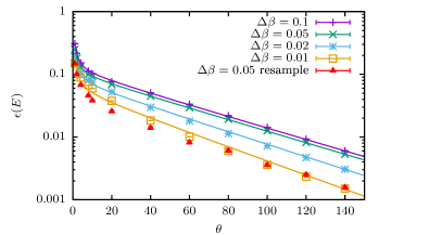
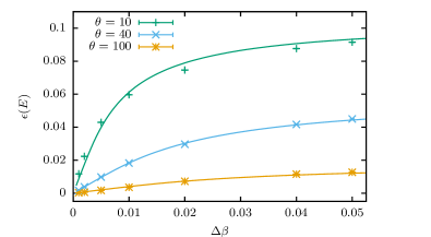
Figure 12: Relative deviation $\epsilon(E)=(E-E_{\mathrm{exact}})/E_{\mathrm{exact}}$ of the internal energy at the critical inverse temperature $\beta_{c}=\frac{1}{2}\ln(1+\sqrt{2})$ for an $L=32$ system sampled in PA runs without resampling on a population of size $R=10\,000$. The results are averaged over $m=200$ independent runs to reduce statistical errors. Top: relative deviation as a function of $\theta$ together with fits of the functional form $\epsilon(E)=ae^{-\theta/\tau_{\mathrm{rel}}}(1+b/\theta)$ motivated by (56) to the data. Bottom: relative deviation as a function of $\Delta\beta$ with fits of the functional form $\epsilon(E)=a\Delta\beta\left(1-e^{-b/\Delta\beta}\right)$.

We first consider the case of the PA algorithm without resampling, where the only source of bias is the relaxation process as the population is cooled in steps. Assume that the population is in equilibrium at inverse temperature $\beta$. If a temperature step $\Delta\beta$ is taken, the system needs to relax towards the new equilibrium energy at $\beta+\Delta\beta$. Assuming a purely exponential relaxation process , the energy will decay as

$$E(t)=\langle E\rangle_{\beta+\Delta\beta}-[\langle E\rangle_{\beta+\Delta\beta}-\langle E\rangle_{\beta}]e^{-t/\tau_{\mathrm{rel}}},$$ (49)

where $\tau_{\mathrm{rel}}=\tau_{\mathrm{rel}}^{E}(\beta+\Delta\beta)$ is the exponential relaxation time of the internal energy at inverse temperature $\beta+\Delta\beta$ Sokal (1997). For sufficiently small temperature steps, a first-order Taylor expansion of the energy as a function of (inverse) temperature implies that Janke (2008a)

$$\langle E\rangle_{\beta+\Delta\beta}-\langle E\rangle_{\beta}\approx\frac{\partial\langle E\rangle}{\partial\beta}\Delta\beta=-\beta^{-2}L^{d}C_{V}\Delta\beta,$$ (50)

and hence we find that the remaining bias $\Delta E$ after $\theta$ sweeps of spin flips is

$$\Delta E=E(\theta)-\langle E\rangle_{\beta+\Delta\beta}\approx\beta^{-2}L^{d}C_{V}\Delta\beta e^{-\theta/\tau_{\mathrm{rel}}}.$$ (51)

To simplify notation, in the following we use $E^{\prime}=\partial E/\partial\beta=-\beta^{-2}L^{d}C_{V}$. For an annealing sweep starting in equilibrium from temperature $\beta_{0}$ (for instance for $\beta_{0}=0$) that arrives at temperature $\beta$, there are remaining biases from all previous temperature steps,

$$\Delta E_{i}=-E^{\prime}_{i}\Delta\beta e^{-\theta/\tau_{\mathrm{rel},i}}+\Delta E_{i-1}e^{-\theta/\tau_{\mathrm{rel},i}},$$ (52)

where $E^{\prime}_{i}=E^{\prime}(\beta_{i})$ refers to the slope of the energy curve at step $i$, and $\tau_{\mathrm{rel},i}=\tau_{\mathrm{rel}}^{E}(\beta_{i})$. Iterating one finds with $\Delta E_{0}=0$ that

$$\Delta E_{i}\approx-\sum_{j=0}^{i-1}E^{\prime}_{i-j}\Delta\beta\,\exp\left[-\theta\sum_{k=0}^{j}1/\tau_{\mathrm{rel},i-k}\right].$$ (53)

While this expression yields the expected bias at inverse temperature $\beta_{i}$, in order to study the dependence on the inverse temperature step $\Delta\beta$, we need to express the bias directly as a function of $\beta$,

$$\Delta E(\beta)\approx-\sum_{j=1}^{n(\beta)}E^{\prime}(\beta_{0}+j\Delta\beta)\Delta\beta\,\exp\left[-\theta\sum_{k=j}^{n(\beta)}1/\tau_{\mathrm{rel},k}\right],$$ (54)

where $n(\beta)=(\beta-\beta_{0})/\Delta\beta$ is the number of temperature steps up to inverse temperature $\beta$. Often one will use small inverse temperature steps $\Delta\beta$ such that we can approximate the sums by integrals to find

$$\Delta E(\beta)\approx-\int_{\beta_{0}}^{\beta}E^{\prime}(\tilde{\beta})\,\exp\left[-\frac{1}{\kappa}\int_{\tilde{\beta}}^{\beta}\frac{{\mathrm{d}}\hat{\beta}}{\tau_{\mathrm{rel}}(\hat{\beta})}\right]{\mathrm{d}}\tilde{\beta},$$ (55)

where $\kappa=\Delta\beta/\theta$ is the cooling rate. Inspecting Eq. (54), we immediately see that to leading order $\Delta E_{i}\sim\Delta\beta$, but note that a change of inverse temperature step changes the whole sequence of the $\beta_{i}$ and hence has additional effects on $\Delta E_{i}$. Considering the dependence on $\theta$, we note that $\Delta E_{i}$ depends on a sequence of exponentials for all higher temperatures, that decay with the harmonic mean of the corresponding relaxation times.

We cannot proceed any further in evaluating the bias of (54) without further simplifying assumptions. In the extreme case where all $\tau_{\mathrm{rel},i}=\tau_{\mathrm{rel}}$ are equal and $E^{\prime}$ is independent of $\beta$, we have from Eq. (54)

$$\begin{split}\Delta E(\beta)&\approx-E^{\prime}\Delta\beta\sum_{j=1}^{n(\beta)}\exp\left[-\frac{\theta}{\Delta\beta\tau_{\mathrm{rel}}}(\beta-[j-1]\Delta\beta)\right]\\ &=-E^{\prime}\Delta\beta\frac{e^{-\theta/\tau_{\mathrm{rel}}}}{1-e^{-\theta/\tau_{\mathrm{rel}}}}\left[1-\exp\left(-\frac{\theta\beta}{\tau_{\mathrm{rel}}\Delta\beta}\right)\right]\end{split}$$ (56)

where we have set $\beta_{0}=0$ for simplicity. We note that while these assumptions are not accurate in general for the 2D Ising model studied here, they will be a good approximation for small $\Delta\beta$ when the rates of change of $\tau_{\mathrm{rel}}$ and $E^{\prime}$ are small. For small inverse temperature steps $\Delta\beta$ the term in square brackets will be negligible. In this case, we expect the $\theta$ dependence to be purely exponential $\Delta E=-E^{\prime}\Delta\beta e^{-\theta/\tau_{\mathrm{rel}}}$ for $\theta/\tau_{\mathrm{rel}}\gg 1$, with a crossover to the inverse linear behavior $\Delta E\approx-E^{\prime}\Delta\beta\tau_{\mathrm{rel}}/\theta$ for $\theta/\tau_{\mathrm{rel}}\ll 1$. Note also that for this simple scenario the form (56) ensures that $\Delta E(\beta_{0}=0)=0$ (which will always be the case by assumption) and bias increases away from $\beta_{0}$ in an exponential fashion to its temperature independent limiting form. Regarding the dependence on temperature step, we see that for small $\Delta\beta$ this is linear, with an exponential crossover to the constant $\Delta E\approx-E^{\prime}\beta(1-\theta/2\tau_{\mathrm{rel}})$ expected in the limit of large steps $\Delta\beta$. In Fig. 12 we show the relative deviation of internal energies at the critical coupling $\beta_{c}$ from the exact result, $\epsilon(E)=(E-E_{\mathrm{exact}})/E_{\mathrm{exact}}$, calculated from PA runs for $L=32$ with resampling turned off. The data have been averaged over $m=200$ runs to reduce statistical errors, such that $\epsilon(E)$ is indeed representative of the systematic error. As is seen from the fits shown together with the data, which are of the form derived above but with independent amplitudes to take account of the approximations involved, the simplified model fits the simulation data very well. The effective relaxation time $\tau_{\mathrm{rel}}=45.4(6)$ (extracted from the fit for $\Delta\beta=0.1$) is comparable, but somewhat smaller than the integrated critical autocorrelation time of $\tau_{\mathrm{int}}=72\pm 14$ extracted from a blocking analysis. Note that in general the bias is not a function of the cooling rate $\kappa$ alone as might be naively assumed, although as the analysis of the simplified form (56) above shows, this is the dependence in certain limiting cases.

We note that while these calculations are for the energy bias $\Delta E$, similar results hold for biases in other quantities with the energy derivative $\partial\langle E\rangle/\partial\beta=-\beta^{-2}L^{d}C_{V}$ replaced by the corresponding derivative of the observable considered and with using the corresponding relaxation times.

VIII.2 Effect of resampling

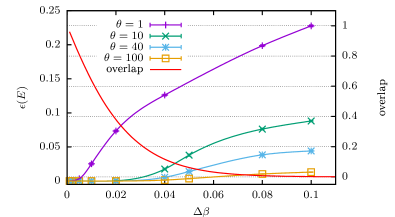
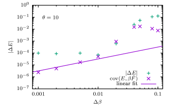
Figure 13: Top: relative deviation $\epsilon(E)=(E-E_{\mathrm{exact}})/E_{\mathrm{exact}}$ of the internal energy at the critical inverse temperature $\beta_{c}$ for an $L=32$ system sampled in PA runs with resampling on a population of size $R=10\,000$ as a function of inverse temperature step $\Delta\beta$. The interpolating lines are merely guides to the eye. The red line shows the exact histogram overlap $\alpha$ at criticality as a function of step size (right scale). Bottom: bias $|\Delta E|=|E-E_{\mathrm{exact}}|$ for the run with $\theta=10$ as compared to the covariance $\operatorname{cov}(E,\beta\hat{F})$ of Eq. (57) together with a linear fit for small values of $\Delta\beta$.

We now turn to the situation of PA with the resampling step enabled. We find that resampling leads to a reduction in bias that is almost independent of the number $\theta$ of equilibration sweeps, such that in this respect it is similar to choosing a reduced inverse temperature step. This is illustrated for $\Delta\beta=0.05$ in the additional data set in the upper panel of Fig. 12. The resampling procedure introduces an additional dependence on the step size $\Delta\beta$ due to histogram overlap as outlined above. To understand this effect, we extend the analysis proposed by Wang et al. Wang et al. (2015a). It was shown there that in the limit of large population sizes the bias $\Delta{\cal O}=\langle\hat{\cal O}\rangle-\langle{\cal O}\rangle$ of an observable ${\cal O}$, i.e., the difference of the expected value of the estimator $\hat{\cal O}$ from PA runs with a given set of parameters and the thermal expectation value of ${\cal O}$, is given by its covariance with the free-energy estimate,

$$\Delta{\cal O}=\operatorname{cov}(\hat{\cal O},\beta\hat{F}).$$ (57)

In Ref. Wang et al. (2015a) it is argued that the size of this bias is essentially determined by the variance $\sigma^{2}(\beta\hat{F})$, namely if one decomposes

$$\Delta\mathcal{O}=\operatorname{cov}(\hat{\cal O},\beta\hat{F})=\sigma^{2}(\beta\hat{F})\left[\frac{\operatorname{cov}(\hat{\cal O},\beta\hat{F})}{\sigma^{2}(\beta\hat{F})}\right],$$ (58)

the quantity in square brackets is claimed to be asymptotically independent of $R$. If and when the estimator $\beta\hat{F}$ of Eq. (33) [together with Eq. (1)] is a sum of many uncorrelated contributions of finite variance stemming from effectively uncorrelated sub-populations, the central limit theorem implies that its variance $\sigma^{2}(\beta\hat{F})\propto 1/R$. In these cases, we can expect the bias in $R$ to decay as $1/R$. We will discuss the numerical findings regarding this behavior below. For completeness, let us mention that it is useful to define the quantity Wang et al. (2015a)

$$\rho_{f}=R\,\sigma^{2}(\beta\hat{F}),$$ (59)

which will attain a finite value in the limit $R\to\infty$ if the above scaling holds. As was discussed above in Sec. VII.2, weighted averages are dominated by outliers for $\sigma^{2}(\beta\hat{F})\gtrsim 1$, and it is hence reasonable to demand that $R\gg\rho_{f}$ for reliable results, justifying the name equilibration population size for $\rho_{f}$ Wang et al. (2015a).

Before turning to our numerical results for the $R$ dependence of bias, we study the dependence of $\operatorname{cov}(\hat{\cal O},\beta\hat{F})$ and $\sigma^{2}(\beta\hat{F})$ on the inverse temperature step $\Delta\beta$. To investigate $\sigma^{2}(\beta\hat{F})$, we note that the estimator (33) is a sum of $i+1$ terms. Neglecting correlations between these terms, the variance of the sum will be the sum of the variances Feller (1968). While the constant $\ln Z_{\beta_{0}}$ does not contribute to the variance, each of the other terms $\delta\beta_{k}\hat{F}_{k}\equiv\ln Q(\beta_{k-1},\beta_{k})$ yields

$$\begin{split}\sigma^{2}(\delta\beta_{k}\hat{F}_{k})&=\sigma^{2}[\ln Q(\beta_{k-1},\beta_{k})]\\ &\approx\sigma^{2}\left[\ln\sum_{j=1}^{R_{k-1}}e^{-\Delta\beta E_{j}}\right],\\ \end{split}$$ (60)

where we have used the fact that the prefactor $R_{k-1}$ in Eq. (1) has only tiny fluctuations or the algorithm could also be formulated for fixed $R_{k-1}=R$. Error propagation implies that to leading order and neglecting correlations between the random variables $E_{j}$, $j=1,\ldots,R_{k-1}$ we have

$$\sigma^{2}(\delta\beta_{k}\hat{F}_{k})\approx(\Delta\beta)^{2}\sum_{j}\frac{e^{-2\Delta\beta E_{j}}}{\left[\sum_{l}e^{-\Delta\beta E_{l}}\right]^{2}}\sigma^{2}(E_{j}).$$ (61)

Since the number of temperature steps up to a given, fixed inverse temperature $\beta$ is inversely proportional to $\Delta\beta$, we find the leading behavior

$$\sigma^{2}(\beta\hat{F})\approx\sum_{k}\sigma^{2}(\delta\beta_{k}\hat{F}_{k})\propto\Delta\beta.$$ (62)

While in reality there will be correlations between the estimates of the different free-energy differences as well as between the energies in the population, we do not expect these to alter the leading scaling behavior. For the covariance $\operatorname{cov}(\hat{\cal O},\beta\hat{F})$ an analogous argument shows that in one step $\operatorname{cov}(\hat{\cal O},\delta\beta_{k}\hat{F}_{k})\propto\Delta\beta$. However, in contrast to $\sigma^{2}(\beta\hat{F})=\operatorname{cov}(\beta\hat{F},\beta\hat{F})$ where ${\cal O}=\beta\hat{F}$ depends on all previous temperature steps, for a “regular” observable ${\cal O}$ such as the energy or magnetization that is a function only of the population at inverse temperature $\beta$, there are no contributions of previous temperature steps to the covariance, and hence the dependence of the total number of temperature steps on $\Delta\beta$ is not relevant for the scaling of $\operatorname{cov}(\hat{\cal O},\delta\beta_{k}\hat{F}_{k})$ with $\Delta\beta$ such that we have

$$\operatorname{cov}(\hat{\cal O},\beta\hat{F})\propto\Delta\beta.$$ (63)

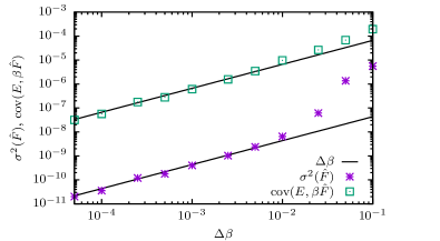
Figure 14: Variance $\sigma^{2}(\beta\hat{F})$ and covariance $\operatorname{cov}(\beta\hat{F},E)$ averaged over the temperature range $0\leq\beta\leq 1$ for $L=32$ as a function of the inverse temperature step $\Delta\beta$. Both scale proportional to $\Delta\beta$ in the limit of small steps as the linear fits illustrate.

To check these predictions of limiting behaviors we performed simulations for a wide range of step sizes $0.5\times 10^{-5}\leq\Delta\beta\leq 10^{-1}$ and MCMC steps $1\leq\theta\leq 200$. The results are summarized in the upper panel of Fig. 13. For larger values of $\Delta\beta$ we find a moderate reduction of bias as compared to the algorithm without resampling (lower panel of Fig. 12), but substantially increased fluctuations. (Note that the topmost data set in the lower panel of Fig. 12 is for $\theta=10$ while that in the top panel of Fig. 13 is for $\theta=1$.) Such increased fluctuations occur due to the loss of diversity in the population induced by the resampling. For $\Delta\beta\geq 0.05$ we have an overlap of energy histograms at inverse temperatures $\beta_{c}$ and $\beta_{c}+\Delta\beta$ of less than 10% (right scale of the top panel of Fig. 13), such that the amount of statistically independent information in the population is reduced by more than a factor of ten in each step — an effect that is only partially made up by the intermediate equilibration sweeps. Only for $\Delta\beta\lesssim 0.02$, is the histogram overlap large enough to counterbalance this effect and lead to a significantly reduced bias without an accompanying increase in statistical fluctuation (cf. also the discussion of the balance of these effects in Appendix A). We note that the histogram overlap decays exponentially away from $\Delta\beta=0$. It is minimal around the critical point and, as one reads off from Fig. 13, for the $L=32$ system it is about $0.3$ for $\Delta\beta=0.02$ at $\beta_{c}$, which could therefore be considered a reasonable maximal inverse temperature step for this case.

To investigate the functional dependence of $\Delta E$ on $\Delta\beta$, consider the lower panel of Fig. 13, where $\Delta E$ from the upper panel is shown for the case of $\theta=10$, but now in a doubly logarithmic plot, displayed together with the expected bias $\operatorname{cov}(E,\beta\hat{F})$ according to Eq. (57). One can distinguish three regimes: for $\Delta\beta\gtrsim 0.04$ the actual bias clearly exceeds $\operatorname{cov}(E,\beta\hat{F})$, indicating that the assumptions made in the derivation leading to the form (57) (in particular the Gaussian nature of fluctuations) are not fulfilled there. For $0.01\lesssim\Delta\beta\lesssim 0.04$, the measured bias agrees with the prediction from the covariance. Finally, for $\Delta\beta\lesssim 0.01$ the bias in the actual simulation drops below the noise level and hence its further reduction cannot be observed. In this latter regime, the predicted bias $\operatorname{cov}(E,\beta\hat{F})$ follows the linear decay $\propto\Delta\beta$ expected from Eq. (63). That the variance $\sigma^{2}(\beta\hat{F})$ as well as the covariance $\operatorname{cov}(E,\beta\hat{F})$ indeed decay proportional to $\Delta\beta$ for sufficiently small steps is more cleanly demonstrated by the data for the temperature-averaged bias presented in Fig. 14 (the dependence on $\Delta\beta$ is found to be uniform in $\beta$), showing the linear decay to hold over several orders of magnitude for sufficiently small $\Delta\beta$ for both quantities. It again turns out to be crucial to ensure sufficient histogram overlap to observe this behavior, which is achieved for $\Delta\beta\lesssim 0.02$ for this system size.

VIII.3 Dependence on population size

It remains to discuss the dependence of systematic errors on the population size. The analysis in Ref. Machta and Ellis (2011) for a double-well model in the absence of any autocorrelations as well as the arguments from Ref. Wang et al. (2015a) discussed in the previous subsection suggesting that $\sigma^{2}(\hat{F})\propto 1/R$ for large $R$ would indicate that bias decays inversely in $R$. To scrutinize the behavior for the PA simulations of the Ising model considered here, in the top panel of Fig. 15 we show the relative deviation in the internal energy, $\epsilon(E)=(E-E_{\mathrm{exact}})/E_{\mathrm{exact}}$, as a function of $R$. In the critical region it decays much more slowly than $1/R$ and one sees hardly any reduction in bias although $R$ is varied over three orders of magnitude. In contrast, the middle panel shows the bias as a function of $\theta$, where corresponding data sets in the two panels belong to calculations with the same computational effort (and the scales on the axes are the same). Here, the decay is fast and consistent with an asymptotically exponential drop as expected. As is illustrated in the bottom panel of Fig. 15 showing the deviation relative to the statistical error, for $\theta\gtrsim 50$ the bias drops below the level of the noise.

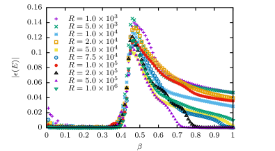
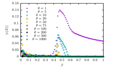
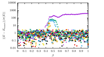
Figure 15: Top: Relative deviation $|\epsilon(E)|=|(E-E_{\mathrm{exact}})/E_{\mathrm{exact}}|$ of the internal energy from PA simulations for $L=64$, $\Delta\beta=0.01$, and $\theta=1$ (heatbath update) and population sizes ranging from $R=10^{3}$ to $R=10^{6}$. Middle: The same bias for a population $R=1000$ for different choices of $1\leq\theta\leq 1000$. Bottom: Energy deviation relative to the statistical error in a logarithmic representation, illustrating that for $\theta\gtrsim 50$, the bias drops below the statistical fluctuations [symbols of data sets as in the middle panel]. Corresponding data sets in all panels amount to the same total computational effort.

It is also instructive to examine the expression for the bias in the “thermodynamic integration limit” $\Delta\beta\to 0$ discussed above. To the extent that the MC is efficient and hence the populations at successive temperature points are not very strongly correlated, one could replace the free-energy estimate $\beta\hat{F}$ in Eq. (57) by the last increment $\beta\Delta\hat{F}$,

$$\Delta{\cal O}\approx\operatorname{cov}(\hat{\cal O},\beta\Delta\hat{F}).$$ (64)

In the limit $\Delta\beta\ll 1$ one then finds from Eqs. (41) and recalling Eq. (20)

$$\begin{split}\Delta{\cal O}&\approx\Delta\beta\operatorname{cov}[\hat{\cal O},\overline{E}(\beta)]=\Delta\beta\sigma^{2}(\overline{E})\frac{\operatorname{cov}(\hat{\cal O},\overline{E})}{\sigma^{2}(\overline{E})}\\ &\approx\Delta\beta\frac{\sigma^{2}(E)}{R_{\mathrm{eff}}}\left[\frac{\operatorname{cov}(\hat{\cal O},\overline{E})}{\sigma^{2}(\overline{E})}\right].\end{split}$$ (65)

Assuming that the term in square brackets has only a weak dependence on $R$ (analogous to the argument used above in Sec. VIII.2), one would conclude that

$$\Delta{\cal O}\propto\frac{1}{R_{\mathrm{eff}}}.$$ (66)

The significance of this observation for the performance of the algorithm is discussed in the following section.

VIII.4 Pure resampling and effective population size

Above, we have considered the PA algorithm and its bias in the absence of resampling. It is also possible and instructive to analyze the method in the opposite limit of a pure resampling method, i.e., for $\theta\to 0$. In this case, the size of the temperature step does not matter as one works only with the configurations of the initial population. Since the resampling factors multiply over different temperature steps,

$$\begin{split}\exp(-\beta_{k}E_{j})=&\exp[-(\beta_{k}-\beta_{0})E_{j}]\\ &=\prod_{i=1}^{k}\exp[-(\beta_{i}-\beta_{i-1})E_{j}],\end{split}$$ (67)

the statistical weight of a configuration of the initial population ($\beta_{0}=0$) at a given lower temperature $\beta_{k}$ is independent of the number (and spacing) of temperature steps taken in between. Due to the normalization of resampling factors, which suppresses fluctuations, the above identity is only approximately realized in the actual PA method, but numerically we find that (for reasonable values of $R$) the results for $\theta=0$ are almost perfectly independent of $\Delta\beta$.

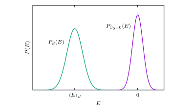
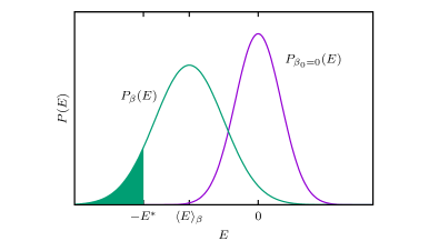
Figure 16: Schematic of energy distributions in $\theta=0$ population annealing. Top: $P_{\beta_{0}=0}$ corresponds to the initial population, $P_{\beta}$ to the distribution at a lower temperature. Bottom: in a finite population of size $R$ at $\beta_{0}=0$, there are typically no replicas with energies lower than $-E^{\ast}$ (and similarly none with energies higher than $E^{\ast}$), where $P_{\beta_{0}}(E^{\ast})=1/R$.

In PA with $\theta=0$, estimating the energy distribution $P_{\beta}(E)$ (or any derived quantity) amounts to reweighting from the distribution at $\beta_{0}=0$. This is in fact just the situation encountered for simple-sampling Monte Carlo, and so the following analysis applies to this problem as well. Because of the finite number $R$ of samples in the histogram $\hat{P}_{\beta_{0}}(E)$, there are no samples with energies very far away from the peak of the distribution at $E=0$. We assume that the width of these histograms is smaller than their distance, cf. the upper panel of Fig. 16. If $P_{\beta_{0}}(E=\langle E\rangle_{\beta})\leq 1/R$, there will essentially be no events in $\hat{P}_{\beta_{0}}(E)$ that have substantial weight in the distribution $P_{\beta}(E)$. In this case, the resampled histogram will be dominated by the few replicas of smallest energies in $\hat{P}_{\beta_{0}}(E)$, and all replicas at inverse temperature $\beta$ will be copies of these few replicas. Hence in this limit we have $R_{\mathrm{eff}}\approx 1$. Since $P_{\beta_{0}}(E)$ is Gaussian (for not too small system size), we can determine $\beta$ for the marginal case by requiring

$$P_{\beta_{0}}(E=\langle E\rangle_{\beta})=\frac{1}{\sqrt{2\pi\sigma_{0}^{2}}}e^{-\langle E\rangle_{\beta}^{2}/2\sigma_{0}^{2}}=\frac{1}{R_{0}},$$ (68)

where $R_{0}$ is the population size starting from which one can expect to find a reasonable result for $P_{\beta}(E)$ without MCMC steps, and $\sigma_{0}^{2}=zL^{d}/2$ with $z=4$ and $d=2$ for the square lattice. In other words, one expects substantial biases to occur as soon as the point from which on there are no entries in the population at $\beta_{0}$ reaches the peak of the distribution at $\beta$. The required population size therefore grows as

$$R_{0}\sim e^{\langle E\rangle_{\beta}^{2}/2\sigma_{0}^{2}},$$ (69)

i.e., exponentially in the total energy $\langle E\rangle_{\beta}\propto L^{d}$. Conversely, for a given population size $R$ strong biases are expected for inverse temperatures $\beta\geq\beta^{\ast}$ where

$$\langle E\rangle_{\beta^{\ast}}^{2}=2\sigma_{0}^{2}\ln\frac{R}{\sqrt{2\pi\sigma_{0}^{2}}}.$$ (70)

This is illustrated in Fig. 17 showing results of PA simulations with $\theta=0$. The vertical lines in the detailed view of the middle panel indicate the values of $\beta^{\ast}$ corresponding to the chosen $R$.

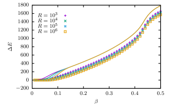
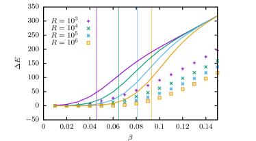
Figure 17: Top: Bias of the (total, not per site) internal energy estimate from PA simulations for $L=32$ and $\theta=0$ and different population sizes. The lines show the conservative bias estimate resulting from Eq. (74). Middle: Detail of the upper panel. The vertical lines indicate the maximum inverse temperature, $\beta^{\ast}$ from which strong biases are expected according to Eq. (70). Bottom: Value of the normalized cut-off energy $e_{<}=(-E^{\ast}-\langle E\rangle_{\beta})/\sigma_{\beta}$.

To understand the behavior of the bias as a function of $\beta$ and $R$, we use a simplified analysis based on the above argument for $R_{0}$ and a Gaussian shape of the energy distribution. If we want to estimate $\langle E\rangle_{\beta}$ from the population at $\beta_{0}$, the above arguments imply that there are no events in the empirical (reweighted) histogram at $\beta$ for energies below $-E^{\ast}$ determined by Eq. (70) for $E^{\ast}=\langle E\rangle_{\beta^{\ast}}$, see the bottom panel of Fig. 16. Hence the PA estimate of the average energy will be systematically too large, namely

$$\hat{E}_{\beta}=\int_{-\infty}^{\infty}\hat{P}_{\beta}(E)E\,\mathrm{d}E\approx\langle E\rangle_{\beta}-\int_{-\infty}^{-E^{\ast}}P_{\beta}(E)E\,\mathrm{d}E.$$ (71)

If we assume that $P_{\beta}(E)$ is Gaussian, which is exact for $\beta=0$, but otherwise will be a good approximation for all temperatures apart from the critical regime, the resulting bias is

$$\begin{split}\Delta E&=\hat{E}_{\beta}-\langle E\rangle_{\beta}=-\int_{-\infty}^{-E^{\ast}}P_{\beta}(E)E\,\mathrm{d}E\\ &=-\frac{1}{\sqrt{2\pi\sigma_{\beta}^{2}}}\int_{-\infty}^{-E^{\ast}}e^{-\frac{(E-\langle E\rangle_{\beta})^{2}}{2\sigma_{\beta}^{2}}}E\,\mathrm{d}E.\end{split}$$ (72)

We note that $\sigma_{\beta}^{2}=C_{V}(\beta)L^{d}/\beta^{2}$, where $C_{V}$ is the specific heat. With the abbreviation

$$e_{<}=(-E^{\ast}-\langle E\rangle_{\beta})/\sigma_{\beta}$$ (73)

we find

$$\begin{split}\Delta E&=-\langle E\rangle_{\beta}\Phi(e_{<})+\frac{\sigma_{\beta}}{\sqrt{2\pi}}\exp(-{e_{<}}^{2}/2)\\ &\equiv\Delta E_{1}+\Delta E_{2}.\end{split}$$ (74)

Here, $\Phi$ denotes the cumulative standard normal distribution function. Figure 17 shows the bias in energy observed from PA simulations with $\theta=0$ performed for the $L=32$ model as well as the estimate from Eq. (74). The latter follows the general behavior of the actual bias, but systematically overestimates it. This is expected, however, as in reality there can be occasional events with energies less than $-E^{\ast}$, just with a probability less than one per energy bin. From the data of Fig. 17 it seems clear that while for very small $\beta\lesssim 0.1$ one can see a decay of bias towards zero, this is not the case for significantly lower temperatures, where the bias is almost unchanged even on increasing $R$ over three orders of magnitude. This is in quite strong contrast to the general law of a $1/R$ decay of bias proposed in Ref. Wang et al. (2015a) (and earlier in Ref. Machta and Ellis (2011)), but in line with the observations for the Ising model shown above in Fig. 15.

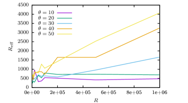
Figure 18: Effective population size $R_{\mathrm{eff}}$ at $\beta=0.44$ as estimated from the blocking analysis for PA runs for $L=64$ and the indicated values of $R$ and $\theta$. For $R<R_{0}(\theta)$, $R_{\mathrm{eff}}$ is essentially independent of $R$, while for $R\geq R_{0}(\theta)$, $R_{\mathrm{eff}}\propto R$.

To understand the $R$ dependence of bias more systematically, we study the functional form of Eq. (74). The behavior crucially depends on the normalized cut-off energy $e_{<}$ of Eq. (73) which according to the bottom panel of Fig. 17 changes sign on moving away from $\beta=0$. This sign-change occurs when the cut-off energy $-E^{\ast}$ coincides with the average energy $\langle E\rangle_{\beta}$, such that beyond that point there are practically no relevant events in the histogram at $\beta_{0}=0$ that would allow to estimate the energy at $\beta$. Hence, any reasonable reweighting can only occur in the regime where $e_{<}<0$. For very small $\beta$, we can use the asymptotic expansion of $\Phi(z)$ abramowitz:book ,

$$\Phi(z)=-\frac{\exp(-z^{2}/2)}{\sqrt{2\pi}z}\left(1-\frac{1}{z^{2}}+\cdots\right),$$ (75)

for $z\to-\infty$ to see that the leading-order $R$ dependence of both $\Delta E_{1}$ and $\Delta E_{2}$ is due to $\sim\exp(-e_{<}^{2}/2)$. On substituting $e_{<}$ from Eq. (73) and using Eq. (70) one finds

$$e^{-e_{<}^{2}/2}=\left(\frac{\sqrt{2\pi\sigma_{0}^{2}}}{R}\right)^{\alpha(R,\beta)}e^{-\langle E\rangle_{\beta}^{2}/2\sigma_{\beta}^{2}},$$ (76)

where the exponent $\alpha(R,\beta)$ is given by

$$\alpha(R,\beta)=\frac{\sigma_{0}^{2}}{\sigma_{\beta}^{2}}-\frac{\sqrt{2\sigma_{0}^{2}}}{\sigma_{\beta}^{2}}|\langle E\rangle_{\beta}|\left(\ln\frac{R}{\sqrt{2\pi\sigma_{0}^{2}}}\right)^{-1/2}.$$ (77)

This is a rather interesting relation: asymptotically, it indicates power-law decay in $1/R$ with an exponent that depends on the ratio $\sigma_{0}/\sigma_{\beta}$ of widths of the corresponding energy distributions. In the limit of small $\beta$ considered here, corresponding to small temperature steps in the $\theta>0$ case, $\sigma_{0}/\sigma_{\beta}\to 1$ and so the bias decays as $1/R$. However, due to the second term in Eq. (77) the crossover to the leading $1/R$ behavior is extremely (logarithmically) slow and, for example, for $R=10^{6}$ and $\beta=0.03$ one finds $\alpha(R,\beta)\approx 0.36$ for $L=32$.

On the other hand, in the limit of large $\beta$, which for the $L=32$ Ising system and population sizes between $10^{3}$ and $10^{6}$ already sets in for $\beta\gtrsim 0.2$ where $e_{<}\gtrsim 5$ and hence $1-\Phi(e_{<})\lesssim 10^{-7}$ (cf. the bottom panel of Fig. 17), $\Phi(e_{<})\approx 1$ to a high accuracy, such that $\Delta E_{1}\approx-\langle E\rangle_{\beta}$, while $\Delta E_{2}$ no longer decays (but note that it is strongly suppressed by a factor $\exp[-\langle E\rangle_{\beta}^{2}/2\sigma_{\beta}^{2}]$). Hence the bias is essentially independent of population size in this regime. Clearly, the onset of this regime gradually shifts to larger $\beta$ for increasing $R$, but according to Eq. (70) this happens logarithmically slowly in $R$.

For a PA simulation with $\theta>0$ the strength of bias effects will depend on the efficiency of the Monte Carlo sweeps. In temperature regions where $\theta\gg\tau_{\mathrm{rel}}$ we will always be in the weak-bias regime and the $1/R$ decay can be observed at least asymptotically. In regions where $\theta\ll\tau_{\mathrm{rel}}$, on the other hand, such as close to the critical point in the Ising model for small values of $\theta$ or big systems, one is in the strong-bias regime found above for $e_{<}>0$, where there is essentially no population-size dependence of the bias within practically achievable population sizes. This is exactly the behavior found for simulations of the Ising model as reported in Fig. 15. Note that this effect only occurs for problems where the energy is a relatively slow mode. For spin glasses this is not the case, and so it is much easier to see the $1/R$ decay of the bias there (see also the data presented in Ref. Wang et al. (2015a)).

Another effect of the tail domination of the resampling weights with a lack of (efficient) MC moves is that for population sizes below $R_{0}$ the resampled population is dominated by copies of one or a few replicas in the parent population that happen to have the lowest energies. In these cases, the effective population size following the discussion in Sec. V.2 is essentially $R_{\mathrm{eff}}\approx 1$ . Hence for $\theta=0$ the effective population size is

$$R_{\mathrm{eff}}=\left\{\begin{array}[]{ll}\approx 1&\mbox{for}\;R\leq R_{0}\\ \mathrm{const.}\times R&\mbox{for}\;R>R_{0}\end{array}\right..$$ (78)

For $\theta>0$ we expect a similar behavior unless the MCMC alone is able to equilibrate the replicas, i.e., we expect $R_{\mathrm{eff}}=R[1-\exp(-\theta/\tau_{\mathrm{eff}})]$ to hold only for $R>R_{0}$. (But note that $R_{0}$ should depend on $\theta$ too in this case.) This is illustrated in Fig. 18 that shows the effective population size as determined from the energy observable for $\beta=0.44$, very close to the critical point. We observe that $R_{\mathrm{eff}}$ is approximately constant and equal to a minimal value (limited by the choice of the number of bins for the blocking analysis which is $B=100$ here) for $R<R_{0}(\theta)$ and only proportional to $R$ for $R\geq R_{0}$. For $\theta=30$, $R_{0}$ appears to be around $R=2\times 10^{5}$.

IX Performance

Population annealing requires only relatively moderate modifications of standard simulation codes that are typically based on MCMC, such as the single-spin flip Metropolis or heatbath dynamics for the Ising model considered here. The main change relates to the simulation of an ensemble of configurations rather than a single copy. The resulting potential for the efficient utilization of highly parallel architectures has been discussed elsewhere Barash et al. (2017a); Christiansen et al. (2019). The computational overhead incurred by the resampling step results from the calculation of the resampling weights $Q$ and $\hat{\tau}_{i}(E_{j})$ of Eqs. (1) and (4), drawing the numbers $r_{i}^{j}$ of copies from the chosen resampling distribution, and the actual copy operations of configurations in memory or, for a distributed implementation, over the network. In shared memory systems this overhead is often rather moderate. For the serial CPU reference code used for the present study, we show a comparison of a PA simulation and the pure single-spin flip code in Fig. 19. At the scale of the total simulation time, no difference is visible for the chosen parameters. As the inset illustrates, the relative overhead of performing the resampling step is below 1% for $L=16$ and dropping to less than 1‰ for $L>128$. For a discussion of the situation on GPU see Ref. Barash et al. (2017a). As here the temperature step was chosen to scale with $L$ as $\Delta\beta=16/75L$ to follow the expected scaling of the histogram overlap in this model Janke (2008a), the overall runtime scales with $L^{3}$ as is illustrated by the straight line in Fig. 19.

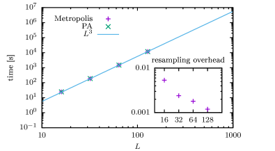
Figure 19: Run times of sample PA simulations for the 2D Ising model and system sizes $L=16$, $\ldots$, $128$ for a population size of $R=5000$, $\theta=10$, $\Delta\beta=16/75L$. The inset shows the relative excess time as compared to simulations with the resampling step turned off.

The algorithmic performance of population annealing as a meta-algorithm is clearly dependent on the model under consideration. For the reference case of the 2D Ising model studied here, we do not expect massive improvements over the underlying MCMC dynamics as the main difficulty in simulating the Ising model’s continuous transition lies in the critical slowing down near the transition, and not in a complex free-energy landscape. The Ising model can in fact be very efficiently simulated with the help of cluster algorithms Swendsen and Wang (1987); Wolff (1989), which can also be combined with PA, but this is not the subject of the present study. Here, instead, we focus on any possible reductions in bias and statistical errors that result from implanting the MCMC into the PA framework. Figure 20 shows the ratio of squared error bars for the specific heat (top) and susceptibility (middle) for simulations using PA as compared to single-spin flip runs with the same statistics. While for most temperatures where the MCMC is easily able to decorrelate configurations the statistics are equivalent leading to a unit ratio of variances, in the critical regime the consideration of an ensemble of configurations together with resampling leads to decreased correlations as compared to the time series of a single MCMC run and hence reduced error bars. The “speedup” displayed in Fig. 20 corresponds to the number of such single-spin flip simulations required to get the statistical errors to the same level as in a single PA run. It is found to reach up to about 10 for the specific heat and up to about 20 for the susceptibility, but no particularly clear scaling behavior is found with increasing the system size. Note that it is crucial for the relatively good performance of the single-spin flip simulations that the final configuration at $\beta_{i-1}$ is used as starting configuration at $\beta_{i}$ (hence these runs correspond to what is called equilibrium simulated annealing in Ref. Rose and Machta (2019)). For the chosen parameter combinations, bias is far below the threshold of statistical error, so we do not provide a detailed comparison of methods in this respect, but overall for the Ising model we do expect the exponential decay of bias with the number of MCMC sweeps as compared to the inverse decay with population size as discussed in Sec. VIII to put the single-spin flip simulations in a position of advantage as compared to PA runs in this respect.

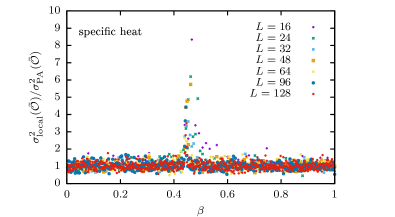
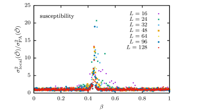
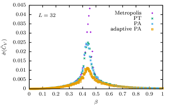
Figure 20: Relative squared error bars of observable estimates from Metropolis temperature sweeps against PA runs with the same number of spin flips. The resulting “speedups” relate to the specific heat (top panel) and the magnetic susceptibility (middle panel), respectively. PA updates are for $R=50\,000$, $\theta=(L/16)^{2}$, $\Delta\beta=16/75L$ and Metropolis runs are for $R=1$, $\theta=50\,000\times(L/16)^{2}$ and the same temperature sequence. Bottom panel: error bar of the specific heat estimate for $L=32$ and Metropolis and parallel tempering simulations as compared to standard and adaptive PA runs.

It is further instructive to compare the effect of the PA meta-heuristic to that of the more established parallel tempering method Geyer (1991); Hukushima and Nemoto (1996). To allow for a relatively fair comparison, we employ the same temperature sequence and the same total number of spin flips. As is clear from the presentation of the results in the bottom panel of Fig. 20, the reduction achieved in statistical errors by applying parallel tempering on top of the Metropolis spin-flip dynamics is practically identical to that seen for PA, at least for the parameters used here. This is in line with previous observations indicating that the algorithmic performance of PA in improving simulations and exploring the state space is quite comparable to that effected by the more traditional parallel-tempering heuristic Wang et al. (2015c, a); Christiansen et al. (2019). In this respect, the main advantage of the PA method must be sought in the far superior parallel scaling in large simulations Christiansen et al. (2019).

There is a great potential for further improvements to the PA method, however, and while these haven been Barash et al. (2017a); Barzegar et al. (2018); Amey and Machta (2018); Barash et al. (2019) and will be Weigel et al. discussed elsewhere, we show for comparison in Fig. 20 the error bars achieved by combining an adaptive temperature schedule Barash et al. (2017a) with overlap $\alpha=0.9$ and an adaptive flip schedule that dynamically modifies $\theta$ to ensure sufficient decorrelation. In addition to the reduction in statistical errors, through the dynamic flip schedule the adaptive simulation needs only about a fifth of the runtime as compared to the other methods.

X Conclusions

We have provided a detailed analysis of the properties of the population annealing algorithm, using as a controlled and generic example the case of the two-dimensional Ising model for which manifold exact and previous numerical results are available. Our focus was on a systematic study of the dependence of systematic and statistical errors on the parameters of the simulation, most notably the population size $R$, the number of rounds of spin flips $\theta$, and the inverse temperature step $\Delta\beta$.

At the core of population annealing is the resampling step that replicates particularly well equilibrated replicas while eliminating those that are not representative of the current temperature, cf. Fig. 1. While selective replication helps to drive the simulation towards equilibrium, the correlations between replicas built up in this process naturally increase statistical errors. On the other hand, they also work towards increasing the fluctuations in the distribution of configuration weights that are responsible for systematic error (bias). The strength of such correlations is hence the central quantity for assessing the quality of approximation. A particularly useful proxy of the actual correlations taking the correlating effect of replication as well as the decorrelation of the Monte Carlo moves into account is given by the effective population size $R_{\mathrm{eff}}$ that can be readily estimated using a standard blocking procedure. For the Ising model, $R_{\mathrm{eff}}(E)$ is dramatically reduced in the critical regime — indicative of the presence of critical slowing down — but can recover in the ordered phase, in contrast to correlation measures based entirely on the analysis of the family tree.

Apart from providing $R_{\mathrm{eff}}$, the blocking and jackknifing procedure also allows for estimates of statistical errors from within a single PA simulation. Such error estimates are reliable as long as $R_{\mathrm{eff}}$ is never less than a few thousand replicas. It should hence be monitored in any PA simulation, preferably for several relevant observables. We established an effective description of the dependence of $R_{\mathrm{eff}}$ on the PA parameters, namely

$$R_{\mathrm{eff}}=R\left[1-\frac{\Delta\beta}{\Delta\beta_{0}}\exp(-\theta/\tau_{\mathrm{eff}})\right],$$

that holds for small $\Delta\beta$ and $R_{\mathrm{eff}}$ satisfying the self-consistency condition. Here, $\tau_{\mathrm{eff}}$ is an effective autocorrelation time that is related to the relaxation time of the underlying MCMC algorithm. By definition, statistical errors decay as $1/\sqrt{R_{\mathrm{eff}}}$.

For systematic errors $\Delta{\cal O}$ (bias), we have provided a description of PA without resampling, where the behavior is determined by the spectrum of relaxation times at all temperature points above the one considered. Including selective replication does not affect the exponential functional dependence on $\theta$, but leads to a much stronger sensitivity with respect to $\Delta\beta$ since alike to the swap moves in parallel tempering it is only in the presence of sufficient overlap of the energy histograms at neighboring temperatures that the resampling works reliably. For small steps the bias is linear in $\Delta\beta$ — we find this to hold numerically and additionally derive it from the relation of bias to the covariance of the considered observable with the free-energy estimator that was previously suggested in Ref. Wang et al. (2015a). Studying this estimator in the limit of small (inverse) temperature steps reveals that it is in fact thermodynamic integration in disguise, and it is possible to understand that in this limit the variance of the free-energy estimator is proportional to $\Delta\beta/R_{\mathrm{eff}}\propto\Delta\beta/R$. These findings can be summarized as

$$\Delta{\cal O}\sim\frac{\Delta\beta}{R_{\mathrm{eff}}}e^{-\theta/\tau_{\mathrm{rel}}}.$$

In practice, however, it can be quite difficult to reach the asymptotic regime where $\Delta{\cal O}\propto 1/R$. In cases where the energy itself is slow to relax and if $\theta$ is too small to keep the population in equilibrium at a given temperature step, $R_{\mathrm{eff}}$ is effectively independent of population size up to large values of $R$. Increasing the size of the population is an extremely inefficient way of improving equilibration in such situations, and instead the only viable option is to increase $\theta$ and/or choose a more efficient MCMC algorithm.

In view of the above, one might wonder how to best choose the simulation parameters $R$, $\theta$ and $\Delta\beta$. Unfortunately, the above relations for statistical error and bias are asymptotic, and hence rules derived from them might not yield the best compromise for a given computational budget. Nevertheless, it is possible to derive a number of guiding principles for the implementation of successful PA simulations:

1. Choose $\Delta\beta$ to (just) ensure sufficient histogram overlap, for instance $\alpha>0.7$. This might involve different inverse temperature steps at different temperatures. Ideally revert to using adaptive stepping Barash et al. (2017a); Amey and Machta (2018).

2. In the regime where the MCMC is efficient, ensure that $\theta$ is chosen large enough to ascertain equilibration of the population at each temperature step. In a regime where the relaxation times become too large — for example on entering a phase of broken ergodicity — spin flips will likely become less relevant Rose and Machta (2019). Potentially choose a more efficient MCMC algorithm if it is available.

3. With any remaining computational resources adapt the population size to bring down statistical errors (that will asymptotically dominate) to the desired level.

4. Monitor $R_{\mathrm{eff}}$ during the course of the simulation, ensuring that it is $\gtrsim 1000$–$5000$ at all times; potentially consider $R_{\mathrm{eff}}$ for different relevant observables, including the configurational overlap.

5. Make use of the potential for extensive parallelization of the algorithm, potentially allowing to arbitrarily reduce statistical and systematic errors of the estimates at the same overall wallclock time if and when sufficient parallel resources are available Weigel (2018).

6. Evaluate statistical errors, including the variance and covariances involving the free-energy estimator using a jackknife block analysis of the tree-ordered population of replicas.

When considering any such general guidelines for optimizing population annealing, it is important to also keep in mind the different levels of relevance of bias and statistical errors in different applications. While in studies of pure systems systematic errors can typically be brought under control by the employment of suitable MCMC algorithms and long runs, the sitution is different for simulations of systems with quenched disorder, where the main source of error are sample-to-sample fluctuations and hence runs for individual disorder configurations are relatively short compared to the relevant relaxation times Wang et al. (2015a). Further, so far unexplored applications might have yet different intricacies.

While the present study delivers a rather detailed picture of the performance of the established population annealing algorithm following Ref. Machta (2010), a range of improvements have already been proposed Barash et al. (2017a); Barzegar et al. (2018); Amey and Machta (2018); Barash et al. (2019), and many more are conceivable, including adaptive $\theta$ and $R$ schedules Weigel et al. , the study of further thermodynamic ensembles Rose and Machta (2019), or generalized resampling schemes Gessert et al. . This flexibility, together with the essentially unlimited potential for parallelization turn population annealing into one of the most versatile and promising generalized-ensemble simulation schemes available.

Appendix A Effective population size

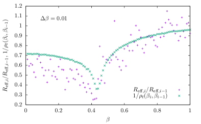
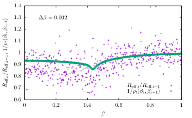
Figure 21: Ratio of effective population sizes before and after the resampling step as compared to the inverse of the one-step mean-square family size according to Eq. (80) for two sizes of the inverse temperature steps ($L=32$, $\theta=20$, $R=50\,000$).

In view of the observed relation Eq. (30) for $R_{\mathrm{eff}}$ it is worthwhile to consider the effect of the individual elements of the algorithm on the effective population size. The resampling step creates identical copies of some replicas while eliminating other members of the population and hence must normally reduce the effective population size. To understand this effect, we consider the variance of the mean. In a population of perfectly uncorrelated members the behavior follows Eq. (19) and hence $R_{\mathrm{eff}}=R$ initially . After resampling (but before applying the spin flips) each copy $k$ of the original population at temperature step $i$ has been replaced by $r^{k}_{i}$ identical copies in the descendant population (where $r^{k}_{i}=0$ for replicas that have died out), cf. Eq. (5). If we assume that $\sigma^{2}({\cal O})$ is the same for all replicas (i.e., the variance is not correlated with the number of children), it is easy to see that the variance of the mean becomes

$$\sigma^{2}(\overline{\cal O})=\sigma^{2}({\cal O})\left(\sum_{k}\frac{{r^{k}_{i}}^{2}}{R^{2}}\right).$$ (79)

It is then natural to define a generalization of the mean square family size $\rho_{t}$ as

$$\rho_{t}(\beta_{j},\beta_{i})=R\sum_{k}{\mathfrak{n}_{k}(\beta_{j},\beta_{i})}^{2},\;\;\;j<i,$$ (80)

where $\mathfrak{n}_{k}(\beta_{j},\beta_{i})$ is the fraction of the population at $\beta_{i}$ coming down from the $k$th member of the population at $\beta_{j}$. Clearly, $\rho_{t}\equiv\rho_{t}(\beta_{0},\beta_{i})$. Since $r^{k}_{i}/R=\mathfrak{n}_{k}(\beta_{i-1},\beta_{i})$, we have

$$\sigma^{2}(\overline{\cal O})=\frac{\sigma^{2}({\cal O})}{R/\rho_{t}(\beta_{i-1},\beta_{i})}.$$

Repeating these arguments for a correlated population with $R_{\mathrm{eff}}<R$, one concludes that after resampling

$$R_{\mathrm{eff},i}=\frac{R_{\mathrm{eff},i-1}}{\rho_{t}(\beta_{i-1},\beta_{i})}.$$ (81)

As is shown in Fig. 21 this relation indeed describes the overall behavior correctly. The deviations, which are particularly visible for $\beta<\beta_{c}$, remind us that the variance (and indeed the mean) of ${\cal O}$ is not necessarily independent of the number of children. In particular, for ${\cal O}=E$ as considered here, we note that such correlations must exist since replicas with lower energies will have more children than those with higher energies.

Note that there should be good reasons to assume that maximizing $\rho_{t}(\beta_{i-1},\beta_{i})$ and hence minimizing the reduction of $R_{\mathrm{eff}}$ through the resampling step should be a desirable goal for choosing among different possible resampling schemes (although the effect on bias is not completely clear at present).

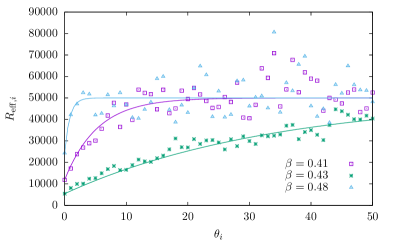
Figure 22: Effective population size $R_{\mathrm{eff},i}$ at inverse temperature $\beta_{i}=0.41$, $0.43$ and $0.48$, respectively, after applying a number of $\theta_{i}$ MCMC steps. The effective population size relaxes to the total population size $R$ according to Eq. (82) as $\theta_{i}$ is increased. The lines show fits of the form (82) with parameter $\tau_{\mathrm{rel},i}$ to the data, the best fit being achieved for $\tau_{\mathrm{rel},i}=5.3$ ($\beta=0.41$), $33.9$ ($\beta=0.43$), and $0.8$ ($\beta=0.48$), respectively ($L=32$, $\theta=10$, $R=50\,000$, $\Delta\beta=0.01$).

After the resampling step that tends to reduce $R_{\mathrm{eff}}$, the spin flips serve to remove some of the correlations in the population. As these are here assumed to be implemented as an MCMC process, such decorrelation will have an exponential time dependence. Focusing on the single leading exponential and taking into account that $R_{\mathrm{eff}}\to R$ as $\theta\to\infty$, the expected behavior is

$$R_{\mathrm{eff},i}=R_{\mathrm{eff},i-1}+(R-R_{\mathrm{eff},i-1})(1-e^{-\theta_{i}/\tau_{\mathrm{rel},i}}).$$ (82)

Here, $\tau_{\mathrm{rel},i}$ denotes the relevant relaxation time at the inverse temperature $\beta_{i}$. This functional form is indeed consistent with the observed data, see the results presented in Fig. 22, showing the behavior of $R_{\mathrm{eff},i}$ as a function of the number $\theta_{i}$ of MCMC steps applied. The lines show one-parameter fits of the functional form (82) to the data, with $R=50\,000$ and $R_{\mathrm{eff},i-1}$ determined after resampling, but before the MCMC steps, via the blocking scheme of Sec. V.2.

From relations (81) and (82) one might deduce conditions for adjusting the population size $R_{i}$ or the number of rounds of spin flips $\theta_{i}$ at each temperature step such as to avoid a possible drop in $R_{\mathrm{eff}}$, but such attempts are left for future work.

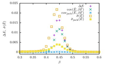
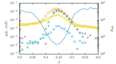
Figure 23: Top: Bias and statistical errors of the average internal energy $\overline{E}$ for the $L=32$ square-lattice Ising model as estimated from independent runs as well as from the jackknife blocking method ($R=50\,000$, $\theta=1$, $\Delta\beta=0.01$). Bottom: The same data in a logarithmic scale shown in comparison to the effective population size $R_{\mathrm{eff}}$ (solid line, right scale).

Appendix B Bias — further numerical observations

Is the bias really represented fully by the covariance with the free-energy estimator? How accurate are the estimates of covariance and variance from the blocking method? These questions are addressed in the plots of Fig. 23 showing the result of a PA run for $L=32$ with a target population size $R=50\,000$ and fixed temperature steps $\Delta\beta=0.01$ with $\theta=1$. Here, we compare for the energy observable (1) the error bars (standard deviation) as estimated from a jackknife block analysis as well as from $m=200$ independent runs, and (2) the bias estimated via $\operatorname{cov}(\overline{E},\beta\hat{F})$, cf. Eq. (57), as determined either from the jackknife or from independent runs with the actual bias as computed via comparison of the simulation data to the exact result Kaufman (1949); Ferdinand and Fisher (1969). Relevant observations are:

• As expected, bias and statistical errors are small everywhere but in the critical region.

• Bias is below statistical error everywhere, even in the critical region, such that (at least for the observable $E$ and for the choice of parameters considered here), a dynamical comparison of bias and statistical error in the sense of an adaptive algorithm would never have suggested to increase $\theta$.

• The covariance with the free energy estimator (as estimated from independent runs) is consistent with the actual bias everywhere. (There might be some small deviations very close to the peak, though.)

• The estimates of both the statistical error and the covariance from the blocking method are consistent with the results from independent runs apart from in the critical regime.

• The deviations of the blocking estimates from the correct results set in exactly when $R_{\mathrm{eff}}$ gets small and hence estimates from blocking can naturally not be trusted.

We note that the data from “independent runs” was produced on GPU while the data for the blocking method are from a CPU run. Since a checkerboard update is used on GPU but sequential updates on CPU, this should lead to slightly different decorrelation properties, which might have resulted in some differences between the shown data sets.

References

- Gramelsberger (2011) G. Gramelsberger, ed., From Science to Computational Sciences: Studies in the History of Computing and Its Influence on Today’s Sciences (diaphanes, Zurich, 2011).
- Janke (2007) W. Janke, ed., Rugged Free Energy Landscapes — Common Computational Approaches to Spin Glasses, Structural Glasses and Biological Macromolecules, Lect. Notes Phys., Vol. 736 (Springer, Berlin, 2007).
- Swendsen and Wang (1987) R. H. Swendsen and J. S. Wang, Phys. Rev. Lett. 58, 86 (1987).
- Wolff (1989) U. Wolff, Phys. Rev. Lett. 62, 361 (1989).
- Berg and Neuhaus (1992) B. A. Berg and T. Neuhaus, Phys. Rev. Lett. 68, 9 (1992).
- Geyer (1991) C. J. Geyer, in Computing Science and Statistics: Proceedings of the 23rd Symposium on the Interface (American Statistical Association, New York, 1991) pp. 156–163.
- Hukushima and Nemoto (1996) K. Hukushima and K. Nemoto, J. Phys. Soc. Jpn. 65, 1604 (1996).
- Wang and Landau (2001) F. Wang and D. P. Landau, Phys. Rev. Lett. 86, 2050 (2001).
- Iba (2001) Y. Iba, Trans. Jpn. Soc. Artif. Intell. 16, 279 (2001).
- Hukushima and Iba (2003) K. Hukushima and Y. Iba, AIP Conf. Proc. 690, 200 (2003).
- Machta (2010) J. Machta, Phys. Rev. E 82, 026704 (2010).
- Wang et al. (2015a) W. Wang, J. Machta, and H. G. Katzgraber, Phys. Rev. E 92, 063307 (2015a).
- Wang et al. (2015b) W. Wang, J. Machta, and H. G. Katzgraber, Phys. Rev. B 92, 094410 (2015b).
- Barash et al. (2017a) L. Y. Barash, M. Weigel, M. Borovský, W. Janke, and L. N. Shchur, Comput. Phys. Commun. 220, 341 (2017a).
- Barash et al. (2017b) L. Y. Barash, M. Weigel, L. N. Shchur, and W. Janke, Eur. Phys. J. Special Topics 226, 595 (2017b).
- Callaham and Machta (2017) J. Callaham and J. Machta, Phys. Rev. E 95, 063315 (2017) .
- Barash et al. (2019) L. Barash, J. Marshall, M. Weigel, and I. Hen, New. J. Phys. 21, 073065 (2019).
- Amey and Machta (2018) C. Amey and J. Machta, Phys. Rev. E 97, 033301 (2018).
- Barzegar et al. (2018) A. Barzegar, C. Pattison, W. Wang, and H. G. Katzgraber, Phys. Rev. E 98, 053308 (2018).
- Christiansen et al. (2019) H. Christiansen, M. Weigel, and W. Janke, Phys. Rev. Lett. 122, 060602 (2019).
- Rose and Machta (2019) N. Rose and J. Machta, Phys. Rev. E 100, 063304 (2019).
- Perera et al. (2020) D. Perera, F. Hamze, J. Raymond, M. Weigel, and H. G. Katzgraber, Phys. Rev. E 101, 023316 (2020).
- Doucet and Johansen (2011) A. Doucet and A. M. Johansen, in Handbook of Nonlinear Filtering, edited by D. Crisan and B. Rozovsky (Oxford University Press, Oxford, 2011) pp. 656–704.
- von der Linden (1992) W. von der Linden, Phys. Rep. 220, 53 (1992).
- Garel and Orland (1990) T. Garel and H. Orland, J. Phys. A 23, L621 (1990).
- Grassberger (1997) P. Grassberger, Phys. Rev. E 56, 3682 (1997).
- Pártay et al. (2014) L. B. Pártay, A. P. Bartók, and G. Csányi, Phys. Rev. E 89, 022302 (2014).
- Doucet et al. (2001) A. Doucet, N. de Freitas, and N. Gordon, eds., Sequential Monte Carlo Methods in Practice (Springer, New York, 2001).
- Weigel (2018) M. Weigel, in Order, Disorder and Criticality, Vol. 5, edited by Y. Holovatch (World Scientific, Singapore, 2018) pp. 271–340.
- Russkov et al. (2021) A. Russkov, R. Chulkevich, and L. N. Shchur, Comput. Phys. Commun. 261, 107786 (2021).
- Machta and Ellis (2011) J. Machta and R. S. Ellis, J. Stat. Phys. 144, 541 (2011).
- (32) D. Gessert, M. Weigel, and W. Janke, in preparation.
- Gentle (2003) J. E. Gentle, Random Number Generation and Monte Carlo Methods, 2nd ed. (Springer, Berlin, 2003).
- Li et al. (2020) Y. Li, W. Wang, K. Deng, and J. S. Liu, preprint arXiv:2004.01975 .
- McCoy and Wu (1973) B. M. McCoy and T. T. Wu, The Two-Dimensional Ising Model (Harvard University Press, Massachusetts, 1973).
- Onsager (1944) L. Onsager, Phys. Rev. 65, 117 (1944).
- Kaufman (1949) B. Kaufman, Phys. Rev. 76, 1232 (1949).
- Ferdinand and Fisher (1969) A. E. Ferdinand and M. E. Fisher, Phys. Rev. 185, 832 (1969).
- Beale (1996) P. D. Beale, Phys. Rev. Lett. 76, 78 (1996).
- Note (1) Here and in the following sections for notational convenience we assume a constant population size even though a resampling scheme with fluctuating population size could be used. It should be clear how to generalize the resulting expressions to cover this case by replacing with at each step.
- Janke (2008a) W. Janke, in Computational Many-Particle Physics, edited by H. Fehske, R. Schneider, and A. Weiße (Springer, Berlin, 2008) pp. 79–140.
- Loison et al. (2004) D. Loison, C. L. Qin, K. D. Schotte, and X. F. Jin, Eur. Phys. J. B 41, 395 (2004).
- Berg (2004) B. A. Berg, Markov Chain Monte Carlo Simulations and Their Statistical Analysis (World Scientific, Singapore, 2004).
- Ren and Orkoulas (2006) R. Ren and G. Orkoulas, J. Chem. Phys. 124, 064109 (2006).
- Wang et al. (2015c) W. Wang, J. Machta, and H. G. Katzgraber, Phys. Rev. E 92, 013303 (2015c).
- Note (2) But note that this incorporates the additional assumption of an absence of correlations between the variance and the family size. In Ref. Wang et al. (2015a) is defined as the limit of Eq. (16\@@italiccorr) for , but a consideration for finite population sizes is more appropriate in our formalism of considering an effective number of independent replicas.
- Sokal (1997) A. D. Sokal, in Functional Integration: Basics and Applications, Proceedings of the 1996 NATO Advanced Study Institute in Cargèse, edited by C. DeWitt-Morette, P. Cartier, and A. Folacci (Plenum Press, New York, 1997) pp. 131–192.
- (48) M. Weigel and W. Janke, Phys. Rev. Lett. 102, 100601 (2009); Phys. Rev. E 81, 066701 (2010).
- Feller (1968) W. Feller, An Introduction to Probability Theory and its Applications, Vol. 1 (John Wiley & Sons, New York, 1968).
- Note (3) Note that we use somewhat sloppy notation here in not clearly distinguishing between probabilistic parameters and their estimates.
- Flyvbjerg and Petersen (1989) H. Flyvbjerg and H. G. Petersen, J. Chem. Phys. 91, 461 (1989).
- Efron and Tibshirani (1994) B. Efron and R. J. Tibshirani, An Introduction to the Bootstrap (Chapman and Hall, Boca Raton, 1994).
- Wolff (1988) U. Wolff, Nucl. Phys. B 300, 501 (1988).
- Janke (2002) W. Janke, in Proceedings of the Euro Winter School “Quantum Simulations of Complex Many-Body Systems: From Theory to Algorithms”, NIC Series, Vol. 10, edited by J. Grotendorst, D. Marx, and A. Muramatsu (John von Neumann Institute for Computing, Jülich, 2002) pp. 423–445.
- Young (2015) A. P. Young, Everything You Wanted to Know About Data Analysis and Fitting But Were Afraid to Ask, SpringerBriefs in Physics (Springer, Berlin, 2015) .
- Note (4) Note that the ratio will always be overestimated if the blocks in the binning analysis are not sufficiently independent. This leads to an approach of the asymptotic form of Eq. (30\@@italiccorr) from above as is seen in Fig. 8.
- Janke (2003) W. Janke, in Computer Simulations of Surfaces and Interfaces, NATO Science Series, II. Mathematics, Physics and Chemistry, Vol. 114, edited by B. Dünweg, D. P. Landau, and A. I. Milchev (Kluwer Academic Publishers, Dordrecht, 2003) pp. 111–135, proceedings of the NATO Advanced Study Institute, Albena, Bulgaria, 9–20 September 2002.
- Landau and Binder (2015) D. P. Landau and K. Binder, A Guide to Monte Carlo Simulations in Statistical Physics, 4th ed. (Cambridge University Press, Cambridge, 2015).
-
Note (5)
To see this, consider the variance of the product . If the population sizes
are uncorrelated, we can approximate
where we used the fact that and . Hence the effect of the additional factors depending on is small whenever , which should normally be the case. - Guo and Jerrum (2017) H. Guo and M. Jerrum, in Proceedings of the Twenty-Eighth Annual ACM-SIAM Symposium on Discrete Algorithms (SIAM, 2017) pp. 1818–1827.
- (61) A. M. Ferrenberg and R. H. Swendsen, Phys. Rev. Lett. 61, 2635 (1988); 63, 1658 (E) (1989); 63, 1195 (1989).
- Note (6) This is, in general, a simplification, but the scaling results derived below are expected to be independent of this assumption.
- (63) M. Abramowitz and I. A. Stegun, eds., Handbook of Mathematical Functions with Formulas, Graphs, and Mathematical Tables (Dover Books on Advanced Mathematics), 9th ed. (Dover Publications, New York, 1972).
- Note (7) Note that for a determination of via the blocking method using blocks the estimate of is (up to fluctuations) bounded by . In this case, the degree of correlation is actually too strong to be determined from the given population and number of blocks.
- (65) M. Weigel, L. Y. Barash, W. Janke, and L. N. Shchur, “Adaptive population annealing algorithm,” in preparation.
- Note (8) As in Sec. V.2 we ignore the effect of fluctuating population size here, but it is straightforward to adapt the resulting expressions to account for this factor.