Optimisation of an active heat engine

Abstract

Optimisation of heat engines at the micro-scale has applications in biological and artificial nano-technology, and stimulates theoretical research in non-equilibrium statistical physics. Here we consider non-interacting overdamped particles confined by an external harmonic potential, in contact either with a thermal reservoir or with a stochastic self-propulsion force (active Ornstein-Uhlenbeck model). A cyclical machine is produced by periodic variation of the parameters of the potential and of the noise. An exact mapping between the passive and the active model allows us to define the effective temperature $T_{eff}(t)$ which is meaningful for the thermodynamic performance of the engine. We show that $T_{eff}(t)$ is different from all other known active temperatures, typically used in static situations. The mapping allows us to optimise the active engine, whatever are the values of the persistence time or self-propulsion velocity. In particular - through linear irreversible thermodynamics (small amplitude of the cycle) - we give explicit formula for the optimal cycle period and phase delay (between the two modulated parameters, stiffness and temperature) achieving maximum power with Curzon-Ahlborn efficiency. In the quasi-static limit, the formula for $T_{eff}(t)$ simplifies and coincides with a recently proposed temperature for stochastic thermodynamics, bearing a compact expression for the maximum efficiency. A point - overlooked in recent literature - is made about the difficulty in defining efficiency without a consistent definition of effective temperature.

I Introduction

In his talk “There is plenty of room at the bottom,” Feynman envisioned a microscopic motor working at small scales, even at the single-atom level Feynamn (1960). Such a motor would be the first step required to achieve the ability of “manipulating and controlling things on a small scale”. Sixty years later, Feynman’s idea has been realised in several experiments and its theoretical implications have been deeply analysed Blickle and Bechinger (2012); Roßnagel et al. (2014); Martinez et al. (2015a).

A motor is a device that delivers mechanical work, for instance by pushing a weight in a given direction. Work is obtained by converting a fraction of energy taken from reservoirs: such a fraction represents the motor’s efficiency. In the microscopic world, the list of available energy reservoirs is not substantially different from the macroscopic scale, i.e. mainly chemical or electro-chemical reservoirs or chemically-induced heat reservoirs . In physics of course the choice of heat reservoirs is the one that better stimulates theoretical research as it involves translating principles of thermodynamics to small scales, far from the thermodynamic limit Martinez et al. (2017). The challenge, with microscopic heat engines, is to achieve optimal control of thermal fluctuations, which are involved not only as energy source and sink (as in macroscopic heat engines) but also spoil the stability and reliability of the delivered work. Microscopic work, and therefore efficiency, are in fact highly fluctuating quantities Verley et al. (2014). The effect, also beneficial, of fluctuations on motor efficiency is one of the most intriguing recent discoveries in the field of stochastic thermodynamics Pietzonka and Seifert (2018).

I.1 Passive microscopic heat engine

Microscopic heat engines have been at the center of theoretical and experimental research in the last decade. They have been realised with colloidal particles in optical traps, for instance in Stirling cycles with isochoric and isothermal transformations Blickle and Bechinger (2012) and Carnot cycles with adiabatic and isothermal transformations Martinez et al. (2015a). The realisation of adiabatic passages (which would require complete isolation of the Brownian particle) is obtained through a protocol where both characteristic volume and temperature of the system are changed in such a way that the entropy of the system is conserved Martinez et al. (2015b). Heat engines have also been realised at the atomic scales, by manipulating a trapped ion Roßnagel et al. (2016). The exploitation, at single-atom level, of so-called quantum squeezed states has also been proposed as a way to circumvent Carnot limit in efficiency Roßnagel et al. (2014). The theoretical research on small-scale engines has involved also the possibility of designing specific cycles with optimal power or efficiency Schmiedl and Seifert (2008). An important challenge, in this field, is going beyond the single-particle limit and achieve control/design of systems made of a small number (e.g. $100-1000$) of particles, which can be meaningful for biophysical applications Cerino et al. (2016).

A severe limitation against a straightforward experimental realisation of a heat engine stems from the difficulty of controlling the temperature with due precision, plagued by the unwanted development of gradients and the presence of large relaxation times Martinez et al. (2017). A typical workaround is to replace the high-temperature reservoir with a source of noise, e.g. an applied noisy voltage as in Blickle and Bechinger (2012); Martinez et al. (2015a). A different fascinating possibility is to consider engines made of a different kind of working substances which stay at an effective temperature different (typically higher) than the environment/solvent Puglisi et al. (2017). This can be achieved by means of active particles, i.e. particles which are self-propelled, for instance bacteria or sperms or active colloids (e.g. Janus particles) Bechinger et al. (2016).

I.2 Active heat engines

Every active particle has its own internal motor which induces, in the presence of a viscous solvent, a typical speed $v_{0}$. Of course $v_{0}$ is unrelated to the thermal speed, that is $v_{0}\neq\sqrt{k_{B}T/m}$ where $T$ is the temperature of the environment, $k_{B}$ is the Boltzmann constant and $m$ is the mass of the particle. Most importantly - considering that active micro-swimmers move through overdamped kinematics - their unconfined diffusivity $D_{a}$ is typically much larger than molecular diffusivity $D$: $D_{a}=\tau_{a}v_{0}^{2}\gg D=k_{B}T/\gamma$, being $\tau_{a}$ the active persistency time and $\gamma$ the viscous drag of the particle Bechinger et al. (2016). This consideration leads naturally to define a diffusivity-based active temperature $T_{D}=\gamma D_{a}/k_{B}\gg T$. The equilibrium limit $\tau\to 0$ is typically taken in such a way that $T_{D}\to T$, which requires $v_{0}^{2}\to D/\tau_{a}$.

First studies and experiments demonstrating the possibility of converting random self-propulsion into directed motion or work have been realised in the realm of active ratchets Leonardo et al. (2010); Sokolov et al. (2010); Vizsnyiczai et al. (2017); Reichhardt and Reichhardt (2017); Pietzonka et al. (2019), which are autonomous engines. In the most recent years several proposals of cyclical heat engines have been done and in few cases also experimentally realised.

In Krishnamurthy et al. (2016) a first example of Stirling engine (two isotherms and two isochores) was obtained, where bacteria were involved as bath and the central system was made of a trapped colloidal particle: an external control of the solvent temperature was reflected in a variation of the average speed (activity) of the bacteria, measured through tracking the position fluctuations of the colloidal particles. The authors verified that iso-thermal transformations (compressions and expansions) were also “iso-active”, i.e. activity did not depend appreciably upon the trap stiffness. The advantage of such a bacterial bath was to achieve a much larger range of effective (active) temperatures than in the passive case.

The concept of an active Stirling engine was investigated in a more recent theoretical study Zakine et al. (2017). The authors show that the performances of the engine depend upon what is the “temperature” which is kept fixed during the iso-thermal transformations: the two considered candidates (here we set $k_{B}=1$) are $T_{var}=k\langle x^{2}\rangle$, as chosen in Krishnamurthy et al. (2016), related to energy in a harmonic potential of stiffness $k$, and the diffusion temperature $T_{D}$ defined above, as proposed in Wu and Libchaber (2000). At equilibrium (ie. for thermal particles at temperature $T$) of course $T_{var}=T_{D}=T$. The authors consider several different models for the bacterial bath (including non-Gaussian effects and/or temporal correlations, i.e. persistency), concluding that if $T_{var}$ is kept constant in iso-thermal transformations then the equilibrium limit for efficiency (given by Carnot value) cannot be surpassed, while different things may happen if $T_{D}$ is adopted for the iso-thermal branches of the cycle.

Other authors Martin et al. (2018) have considered a different theoretical model where the central particle is a self-propelled particle (pushed by a random force with exponentially decaying autocorrelation - with typical time $\tau_{a}$ - as in AOUP model, see below) immersed in a bath of passive particles. The authors consider both Stirling type engines (cyclical modulation of temperature and stiffness at fixed $\tau_{a}$) and engines with modulation of $\tau_{a}$ and stiffness, at fixed temperature. Of course the second case has not a passive counterpart and therefore there is no direct way to compare performances. It is important to stress that the authors, here, have decided to connect the thermal bath temperature to the self-propulsion speed, similar to what happens in Krishnamurthy et al. (2016), making more difficult to disentangle their contributions.

In Saha and Marathe (2019) a new heat engine is proposed where a passive particle is trapped in a harmonic potential with time-dependent stiffness and is put in contact with a thermal bath in the first half of the cycle and with an active bath (time-persistent noise) in the second half. In this paper the relevance of $T_{var}$ as a sort of effective temperature and a general equation for its evolution - for a broad class of choices of the driving noise - is shown (an equation discussed in greater detail in the later Holubec et al. (2020)).

In Kumari et al. (2020) a Stirling engine is considered where the central substance is a particle that changes its nature during the cycle itself, i.e. it is passive for three of the four steps, and is an active Ornstein-Uhlenbeck particle (AOUP) during the fourth step which is the isothermal compression. In this paper a higher efficiency (with respect to the passive case) is claimed when activity is present, a fact which evidently depends upon the chosen definition of efficiency.

In Ekeh et al. (2020) the authors consider a model with many active Brownian particles (ABP, i.e. such that their self-propulsion velocity has fixed magnitude and diffusing orientation). The external potential (which also act on propulsion’s orientation) has many parameters that can be varied. The presence of many potential’s parameters allows one to design cycles without changing other properties (such as bath temperature or properties of the activity). Efficiency appears to be proportional to the extracted power and both are optimal together.

We conclude this overview of the very recent literature with Holubec et al. (2020), where the authors propose a general mapping from an active heat engine to a passive heat engine. The mapping can be made explicit when the confining potential is harmonic, and this can be done for whatever model of self-propulsion is proposed: only the auto-correlation of the self-propulsion affects the evolution of the effective temperature. The authors give explicit examples of their formalism using an ABP particle in a harmonic trap, where a Stirling-like cycle is operated by tuning stiffness, temperature and parameters of activity (both speed and persistency time). The important point raised by the authors, also relevant for the interpretation of the experiments in Krishnamurthy et al. (2016), is that the effective temperature may change also during the (apparently) “isothermal” transformations, because it depends upon all the system’s parameters.

I.3 This paper

Here, we propose a study which is complementary to that done in Holubec et al. (2020). We consider AOUP particles which have a natural mapping to passive systems with an active temperature, $T_{a}$(t), which in fact depends upon the potential’s parameters, in the low persistence limit. A recent study of entropy production for AOUP particles also revealed the existence of a Clausius relation that connects entropy changes with a an active heat flow divided by a temperature $T_{cl}(t)$ Marconi et al. (2017); Puglisi and Marconi (2017). Our main point is that the proper effective temperature, $T_{eff}(t)$, relevant for the thermodynamic behaviour of the engine, can be quite different from $T_{a}(t)$ and $T_{cl}(t)$, as well as from other temperatures such as $T_{var}$, $T_{D}$ or $T_{a}$. Later, in Table 1 we summarise some of the most used definitions of temperatures in this context.

The knowledge of the correct effective temperature is crucial to optimize the engine’s performance, for instance of its delivered power. As an explicit application of this concept, we show how to achieve maximum power by tuning $T_{eff}$ through the control of self-propulsion speed, a possibility which has been experimentally realised, recently, with light-controlled bacteria Vizsnyiczai et al. (2017); Arlt et al. (2019) and colloids Schmidt et al. (2019).

Let us summarise the structure of the paper. In Section II we introduce a few standard thermodynamic tools which are useful for finite-size/time thermodynamics (i.e. when models are stochastic and the period of a cyclic transformation is not infinite): in this Section we briefly discuss the correct definition of heat flow coming from the high-temperature thermostat, which is important already for non-active systems, and becomes even more important for active heat engines where the temperature is not directly under control. In Section III we present the passive and active models investigated in the paper, showing the mapping that brings them to be equivalent from the point of view of heat engine performances Holubec et al. (2020). In Section IV we study the periodic heat engine model with only passive particles, particularly in the limit of linear irreversible thermodynamics, deriving a few results which are complementary to those given for the same model in Brandner et al. (2015). In Section V we show how to transfer the knowledge of the passive engine to optimise the active one. In the last section we draw conclusions and perspectives.

II Work and heat for microscopic (passive) heat engines

In the context of microscopic engines, basic thermodynamic concepts, such as heat and work, need a definition in terms of stochastic quantities, even if only averages are needed. For simplicity we consider models with a single (passive or active) particle in a solvent fluid which is viscous enough to make inertia negligible. The particle therefore obeys dynamical equations which result from some external potential $\mathcal{H}({\bf x},{\bf\lambda}_{t})$, thermal fluctuations and self-propulsion (in the active case). An external agent can control the parameters ${\bf\lambda}_{t}$ of the potential and also the properties of the thermal bath and the active self-propulsion: in doing so, it performs or extracts work. In stochastic thermodynamics the definition of stochastic work injection rate (or injected power), is related to the variation of the external potential, i.e. Seifert (2012):

$$\dot{W}=\sum_{i}\frac{\partial\mathcal{H}}{\partial\lambda_{i}}\lambda_{i}=\frac{\partial\mathcal{H}}{\partial t}.$$ (1)

A way to verify the consistency of this relation with thermodynamics Jarzynski (2007) is to study what happens in the quasi-static limit when no active forces are present. This amounts to consider the limit $t_{F}\to\infty$ (where $t_{F}$ is the duration of the transformation). In this limit the system is constantly close to its equilibrium distribution $p_{0}$ at given potential’s parameters ${\bf\lambda}_{t}$, where

$$p_{0}=\frac{1}{\mathcal{Z}({\bf\lambda}_{t})}e^{-\beta\mathcal{H}({\bf x},{\bf\lambda}_{t})},$$ (2)

with

$$\mathcal{Z}({\bf\lambda}_{t})=\int d{\bf x}e^{-\beta\mathcal{H}({\bf x},{\bf\lambda}_{t})}$$ (3)

and $\beta$ the inverse temperature. In particular one has

$$\partial_{t}p_{0}=-\beta\big{[}\partial_{t}\mathcal{H}\big{]}p_{0}-\frac{\partial_{t}\mathcal{Z}(\lambda_{t})}{\mathcal{Z}(\lambda_{t})}p_{0}=\mathcal{O}\Big{(}\frac{1}{t_{F}}\Big{)},$$ (4)

and therefore, according to definition (1), the average work done in the quasi-static limit corresponds - as expected - to the free energy variation

$$\int\big{[}\partial_{t}\mathcal{H}\big{]}p_{0}d{\bf x}=\partial_{t}\Big{[}-\frac{1}{\beta}\ln\mathcal{Z}(\lambda_{t})\Big{]}+\mathcal{O}\Big{(}\frac{1}{t_{F}}\Big{)}.$$ (5)

Instantaneous heat exchange is defined for complementarity from work, i.e.

$$\dot{Q}=\frac{dH}{dt}-\dot{W},$$ (6)

so that the first principle is guaranteed. When the parameters $\lambda_{t}$ are tuned according to a cyclical protocols, i.e. $\lambda_{t+t_{cycle}}=\lambda_{t}$ with $t_{cycle}$ the machine period, most of the models and the initial conditions lead to a limit cycle where averages are periodic with the same period $t_{cycle}$. It is then meaningful to consider the average work integrated in a period

$$W_{p}=\int_{t_{0}}^{t_{0}+t_{cycle}}dt\langle\dot{W}\rangle,$$ (7)

(where $t_{0}$ is a time large enough to consider the system in the limit cycle). We recall that $W_{p}$ - in our notation - must be negative to have a working machine.

II.1 Adsorbed heat

For the purpose of computing the engine’s efficiency, it is crucial to define a measure of energy consumption through heat:

$$Q_{h}=\int_{t_{0}}^{t_{0}+t_{cycle}}dtw_{ads}(t)\langle\dot{Q}\rangle,$$ (8)

where $w_{ads}(t)\in[0,1]$ is a (periodic) weighting function that discriminates how much heat is to be considered as energy gain, while the remaining fraction $1-w_{ads}(t)$ is to be considered as dissipation.

We believe that a good choice (and a good understanding) of $w_{ads}(t)$ - even in the framework of passive, not active, particles - deserves a brief discussion, since it seems that there is not unanimous agreement about it in the literature, even the recent one. In Carnot’s original heat engine, there are two well defined thermostats, i.e. the one at high temperature $T_{h}$ and the one at low temperature $T_{c}$, with adiabatic connections: then, heat is only adsorbed when in contact with $T_{h}$ and is only released when at $T_{c}$. This means that one can safely set

$$w_{ads}(t)=\Theta[\langle\dot{Q}\rangle(t)],$$ (9)

where $\Theta$ is the Heaviside theta function Martinez et al. (2015a, b). However, in more general cases, definition (9) has drawbacks. For instance the Stirling engine - even in the quasi-static limit - exchanges heat during the isochoric branches of the cycle, when in contact with intermediate values $T_{c}<T(t)<T_{h}$: if Eq. (9) is adopted, then $Q_{h}$ takes a contribution also from one of the isochores and the quasi-static efficiency is, in general, smaller than the Carnot one Blickle and Bechinger (2012); Zakine et al. (2017). Such a definition is also problematic from the conceptual point of view, since $Q_{h}$ should be related to heat flowing from a thermostat to a different one, however Eq. (9) gives $Q_{h}>0$ also when there is a single thermostat, i.e. when $Q_{h}$ comes from the same thermostat which - considering the whole transformation - dissipates heat: this happens in several examples with a time-dependent Hamiltonian (periodically modulated potential energy) at a constant temperature. Notwithstanding this drawbacks, definition (9) is frequently adopted Blickle and Bechinger (2012); Krishnamurthy et al. (2016); Zakine et al. (2017); Martin et al. (2018) .

An alternative recipe is offered in Brandner et al. (2015); Cerino et al. (2016), adopted by us in the present study:

$$w_{ads}(t)=\frac{\beta(t)-\beta_{c}}{\beta_{h}-\beta_{c}},$$ (10)

where $\beta(t)=1/T(t)$, $\beta_{c(h)}=1/T_{c(h)}$. This definition weighs more heat (whatever its sign) coming from higher temperature. Eq. (10) is justified by splitting the entropy production into two contributions that depend upon two different thermodynamic forces, one related to the variation of potential energy (which generates work) and one related to the variation of temperature (which generates a heat flux $Q_{h}$ going through the system from high to low temperature) Brandner et al. (2015). Such a recipe also guarantees that in the quasi-static limit the Carnot efficiency $\eta_{c}=1-T_{c}/T_{h}$ is always reached, including the Stirling engine .

Once work and adsorbed heat are defined, one can define the average power

$$P=\frac{W_{p}}{t_{cycle}},$$ (11)

and the average efficiency

$$\eta=-\frac{W_{p}}{Q_{h}}.$$ (12)

II.2 Active-passive equivalence

A fundamental observation can be done for harmonic potentials, i.e. when

$$\mathcal{H}(t)=\frac{1}{2}k(t)x^{2}(t).$$ (13)

For such a choice, work (and total heat which is the opposite of work, in a period) are known through the knowledge of $\sigma(t)=\langle x^{2}\rangle$ and $k(t)$ only Holubec et al. (2020):

$$W_{p}=\int_{t_{0}}^{t_{0}+t_{cycle}}dt\frac{1}{2}\dot{k}(t)\sigma(t),$$ (14)

The same holds true for the instantaneous total heat $\langle\dot{Q}\rangle$, see Eq. (6) as well as for its integral over a period. On the contrary, and at variance with what concluded in Holubec et al. (2020), adsorbed heat

$$Q_{h}=\int_{t_{0}}^{t_{0}+t_{cycle}}dtw_{ads}(t)\frac{1}{2}k(t)\dot{\sigma}(t)$$ (15)

in general does not depend only upon $\sigma(t)$ and $k(t)$, since the definition of $w_{ads}(t)$ could depend upon other parameters, for instance - in the definition adopted by us, Eq. (10) - it depends upon $T(t)$.

III Particle models

In this section we discuss the model of active (and passive) particle and the adopted cycle for the heat engine we want to study. We stick to a harmonic potential with time-dependent stiffness and we adopt the AOUP model for self-propulsion.

III.1 Passive model

As a reference, we consider first an overdamped passive particle with time-dependent diffusivity $D(t)=\frac{k_{B}T(t)}{\gamma}$. We choose units such that the viscous drag $\gamma$ and the Boltzmann constant $k_{B}$ are both set to $1$. The model then reads

$$dx(t)=-k(t)x(t)dt+\sqrt{2T(t)}dw(t),$$ (16)

where $x(t)$ is particle’s position at time $t$, $k(t)$ is the time-dependent harmonic stiffness, and $dw(t)$ is the infinitesimal increment of the Wiener process. The model has been studied in details in Schmiedl and Seifert (2008). The model has a Gaussian propagator and - in the absence of drifts and initial displacements - its dynamics is fully described by the variance of the position $\sigma(t)$ which obeys:

$$\dot{\sigma}(t)=-2k(t)\sigma(t)+2T(t).$$ (17)

In the quasi-static limit of $t_{cycle}\to\infty$, one can change the time-variable in Eq. (17) defining $s=\frac{t}{t_{cycle}}$ (so that in $s$ the period is $1$) and obtaining

$$-2k(s)\sigma(s)+2T(s)=\mathcal{O}(1/t_{cycle}).$$ (18)

which of course in the limit $t_{cycle}\to\infty$ gives $\sigma(t)=\frac{T(t)}{k(t)}$.

III.2 AOUP active model

The AOUP model is considered a good description for a colloid in a bath of swimmers such as bacteria Maggi et al. (2015). This model has some properties in common with the ABP model, for instance the exponentially decaying time-correlation of the cartesian components of the self-propulsion force (but ABP has non-Gaussian fluctuations and therefore it is more complicate to get analytical results). The AOUP model has the advantage of being more accessible to calculations, in particular it has a very well studied approximation in the passive limit (see below), where – in the case of constant parameters – it is mapped into a passive model. We will see, however, how this mapping is not the proper one to understand the performance of this model as a heat engine.

We consider non-interacting AOUP particles (in one dimension) in the hypothesis of large viscosity, that is inertia is neglected and the dynamics is overdamped. We also neglect the thermal noise (which has a small effect with respect to activity), writing :

$$\begin{cases}dx(t)=[-k(t)x(t)+f_{a}(t)]dt\>\>\\ df_{a}(t)=-\frac{1}{\tau_{a}}f_{a}(t)+\frac{{2D_{a}}^{1/2}}{\tau_{a}}dw(t).\end{cases}$$ (19)

The role of self-propulsion is played by $f_{a}(t)$ which is a coloured noise with exponentially decaying time-correlation:

$$\langle f_{a}(t)f_{a}(s)\rangle=\frac{D_{a}}{\tau_{a}}e^{-(t-s)/\tau_{a}},$$ (20)

modelling a force which remains persistent for a time of order $\tau_{a}$. The self-propulsion model has two parameters: the persistence time $\tau_{a}$ and the active diffusivity $D_{a}$. In the absence of external potential and if $D_{a}$ is constant, at large times $t\gg\tau_{a}$, the particle displays normal diffusivity with coefficient $D_{a}$. From it one can define the average self-propulsion speed $v_{0}(t)=\sqrt{D_{a}(t)/(\tau_{a})}$. The passive model is recovered taking $\tau_{a}\to 0$ and $v_{0}(t)\to\infty$ with $D_{a}\to D$. The more general case we consider is a time-dependent $D_{a}(t)$ or $v_{0}(t)$, a situation which has been demonstrated experimentally, for instance in Vizsnyiczai et al. (2017).

The model, being the external potential harmonic, is again a Markovian diffusive model with Gaussian propagator. Again, in the absence of drifts and initial displacements, the dynamics is fully described by the entries of the covariance matrix, that obey the following system of coupled equations:

$$\frac{d{\langle f_{a}^{2}\rangle}}{dt} =-\frac{2}{\tau_{a}}\langle f_{a}^{2}\rangle+\frac{2v_{0}^{2}}{\tau_{a}}$$ (21a)

$$\frac{d{\langle xf_{a}\rangle}}{dt} =\langle f_{a}^{2}\rangle-\frac{1+\tau_{a}k}{\tau_{a}}{\langle xf_{a}\rangle}$$ (21b)

$$\frac{d{\langle x^{2}\rangle}}{dt}=\dot{\sigma}= -2k{\langle x^{2}\rangle}+2{\langle xf_{a}\rangle}$$ (21c)

The latter is equivalent to Eq. (15) of Holubec et al. (2020) and defines - for direct comparison with Eq. (17) - the effective temperature

$$T_{eff}(t)=\langle xf_{a}\rangle(t),$$ (22)

that is the temperature of the passive system which gives the same $\sigma(t)$ and therefore the same delivered work or power. Remarkably, this expression of $T_{eff}$ is directly proportional to the kinetic temperature $T_{kin}=m\langle v^{2}\rangle/d$ (where $d$ is the dimensionality) recently calculated in a static harmonic potential for an inertial AOUP model Caprini and Marini Bettolo Marconi (2021). Interestingly, it is also proportional to the so-called swim pressure Takatori et al. (2014); Winkler et al. (2015).

In the present case, $T_{eff}(t)$ obeys quite a simple differential equation, i.e. (from joining together equations (21a) and (21b))

$$\ddot{T}_{eff}+\left(\frac{3+\tau_{a}k(t)}{\tau_{a}}\right)\dot{T}_{eff}+\\ +\left[\dot{k}(t)+2\frac{1+\tau_{a}k(t)}{\tau_{a}^{2}}\right]T_{eff}(t)-2\frac{v_{0}^{2}(t)}{\tau_{a}}=0,$$ (23)

which represents a central result of this paper. In the passive limit $\tau_{a}\to 0$ with $\tau_{a}v_{0}^{2}(t)\to D_{a}(t)$ the above equation gives the correct expectation $T_{eff}(t)\to T_{D}(t)$. However, already at first order in $\tau_{a}$, one has $T_{eff}(t)\neq T_{D}$.

When the parameters are constant or vary very slowly ($\omega=2\pi/t_{cycle}\to 0$ as done in Eq. (18)), the system reaches a (steady or quasi-static) state where

$$\langle f_{a}^{2}\rangle(t) =v_{0}^{2}(t)$$ (24a)

$$\langle xf_{a}\rangle(t) =T_{eff}(t)=\frac{v_{0}^{2}(t)\tau_{a}}{1+\tau_{a}k(t)}$$ (24b)

$$\langle x^{2}\rangle(t) =\sigma(t)=\frac{v_{0}^{2}(t)\tau_{a}}{k(t)[1+\tau_{a}k(t)]}=\frac{T_{eff}(t)}{k(t)}.$$ (24c)

It is useful to stress that, even in the quasi-static limit (very slow transformations), $T_{eff}(t)\neq T_{D}(t)$ if $\tau_{a}>0$, i.e. if the system is active. In other terms, even with very slow transformations, an active system has a different thermodynamics with respect to a passive one. Interestingly in the recent literature a temperature equal to $T_{eff}$ in the quasi-static limit, $T_{cl}=\frac{v_{0}^{2}\tau_{a}}{1+\tau_{a}k}$ has shown to bear thermodynamic properties, as it underlies a Clausius relation for the entropy change of active particles Marconi et al. (2017); Puglisi and Marconi (2017).

We conclude this section remarking that the meaning of the effective temperature $T_{eff}(t)$ is twofold: first it is the temperature which - replaced into $T(t)$ in the passive model Eq. (16) - gives the same evolution of $\sigma(t)$ in the presence of the same protocol $k(t)$, which guarantees that work, heat and power are exactly the same; second, in the steady state (and in quasi-static transformations) it rules the Boltzmann distribution $p(x)\sim e^{-k(t)x^{2}/T_{eff}(t)}$.

III.3 An approximation for small persistency

It is easy to show Maggi et al. (2015) that the model in (19) can be mapped, without any approximation to a Klein-Kramers model with an effective mass $\tau_{a}$, a harmonic force with an effective stiffness $\dot{k}+\frac{k}{\tau_{a}}$ and a viscous bath with effective drag coefficient $1+\tau_{a}k(t)$:

$$\begin{cases}dx=vdt\\ dv=-\frac{\Gamma(t)}{\tau_{a}}vdt-\left(\dot{k}+\frac{k}{\tau_{a}}\right)xdt+\sqrt{\frac{2v_{0}^{2}(t)}{\tau_{a}}}dw\end{cases},$$ (25)

with

$$\Gamma(t)=1+\tau_{a}\partial_{x}^{2}\mathcal{H}=1+\tau_{a}k(t).$$ (26)

Again, the model has a Gaussian propagator and its dynamics is described by the coefficient of the covariance matrix:

$$\begin{cases}\frac{d\langle v^{2}\rangle}{dt}=-\frac{2\Gamma(t)}{\tau_{a}}\langle v^{2}\rangle+2\frac{\tau_{a}\dot{k}+k}{\tau_{a}}\langle xv\rangle+\frac{2v_{0}^{2}}{\tau_{a}}\\ \frac{\langle xv\rangle}{dt}=\langle v^{2}\rangle+\frac{\Gamma(t)}{\tau_{a}}\langle xv\rangle-\frac{\tau_{a}\dot{k}+k}{\tau_{a}}\langle x^{2}\rangle\\ \frac{\langle x^{2}\rangle}{dt}=2{\langle xv\rangle}\end{cases}$$ (27)

whose steady (or quasi-static) state reads

$$\begin{cases}\langle v^{2}\rangle(t)=\frac{v_{0}^{2}(t)}{\Gamma(t)}=\frac{T_{cl}(t)}{\tau}\\ \langle xv\rangle=0\\ \langle x^{2}\rangle(t)=\frac{v_{0}^{2}(t)\tau_{a}}{k(t)\Gamma(t)}=\frac{T_{cl}(t)}{k(t)}.\end{cases}$$ (28)

In the limit of $\tau_{a}\to 0$, the model in Eqs. (25) can be approximated by a heuristic procedure, equivalent to overdamping, where “inertia” (i.e. $dv$ ) is neglected. This procedure generalises to the case of time-dependent parameters the so-called UCNA expansion Jung and Hänggi (1987); Hänggi and Jung (1995)) and (for the case of a harmonic potential) gives

$$dx=-\frac{\tau_{a}\dot{k}+k}{1+\tau_{a}k}xdt+\sqrt{\frac{2v_{0}^{2}\tau_{a}}{(1+\tau_{a}k)^{2}}}dw.$$ (29)

For simplicity, in the rest of the paper we call this model ”dynamical UCNA” approximation. We notice that it is equivalent to passive model, Eq. (16), and therefore has variance satisfying Eq. (17), with $k(t)$ and $T(t)$ replaced by

$$k_{a}(t) =\frac{\tau_{a}\dot{k}(t)+k(t)}{1+\tau_{a}k(t)},$$ (30a)

$$T_{a}(t) =\frac{v_{0}^{2}(t)\tau_{a}}{(1+\tau_{a}k(t))^{2}}.$$ (30b)

We highlight that $T_{a}(t)\neq T_{eff}(t)$, even at first order in $\tau_{a}$. Of course in the passive limit ($\tau_{a}\to 0$ and $v_{0}^{2}(t)\tau_{a}\to D_{a}(t)$) both temperatures $T_{a}(t)$ and $T_{eff}(t)$ go to $T_{D}(t)$.

In the steady or quasi-static regime (constant or very slowly varying $k(t)$ and $v_{0}(t)$), $T_{a}(t)$ and $T_{eff}(t)$ are still different, even at first order in $\tau_{a}$:

$$T_{eff}(t) \approx\tau_{a}v_{0}^{2}\left[1-k(t)\tau_{a}+\mathcal{O}(\tau_{a}^{2})\right]$$ (31a)

$$T_{a}(t) \approx\tau_{a}v_{0}^{2}\left[1-2k(t)\tau_{a}+\mathcal{O}(\tau_{a}^{2})\right]$$ (31b)

However $\sigma(t)=T_{a}(t)/k_{a}(t)$ coincides with that in Eq. (24c). For small $\tau_{a}$, it takes the form

$$\sigma=\frac{v_{0}^{2}\tau_{a}}{k}(1-\tau_{a}k)+\mathcal{O}(\tau_{a}^{3}).$$ (32)

It is important to understand that the ”passive” problem with parameters $k_{a}(t)$ and $T_{a}(t)$ is not thermodynamically equivalent to our original active problem, since the work (and therefore power) of the original problem must be evaluated against the original stiffness $k(t)$ and not against $k_{a}(t)$. Therefore the analogy appearing in Eq. (29) cannot be immediately used for optimisation purposes. In Table 1 we resume the main definition of temperatures used in this paper. We also summarise, in Table 2, the important physical limits which can be considered when discussing active heat engines.

Name	Definition	Application
$T_{D}$	$\gamma D_{a}/k_{B}$	free diffusion Bechinger et al. (2016)
$T_{var}$	$k\langle x^{2}\rangle/k_{B}$	steady states Krishnamurthy et al. (2016)
$T_{kin}$	$m\langle v^{2}\rangle/k_{B}$	steady states with inertia Caprini and Marini Bettolo Marconi (2021)
$T_{a}(t)$	$\frac{\gamma}{k_{B}}\frac{v_{0}^{2}(t)\tau_{a}}{[1+\tau_{a}k(t)]^{2}}$	dynamical UCNA Maggi et al. (2015)
$T_{cl}(t)$	$\frac{\gamma}{k_{B}}\frac{v_{0}^{2}(t)\tau_{a}}{1+\tau_{a}k(t)}$	Clausius relation Marconi et al. (2017); Puglisi and Marconi (2017) (and $\lim_{\omega\to 0}T_{eff}(t)\;$)
$T_{eff}(t)$	see Eq. (23)	heat engines Holubec et al. (2020).

Table 1: A table with the main definitions of effective temperatures used in the context of active particle models (in one dimension). We recall that $\gamma$ is the viscous drag coefficient and $k_{B}$ the Boltzmann constant, both set to $1$ throughout the paper.

Name	Definition
Passive limit	$\tau_{a}\to 0$, $v_{0}\to\infty$, $\tau_{a}v_{0}^{2}\to D_{a}$
Quasi-static limit	$t_{cycle}\to\infty$ ($\omega\to 0$)
Linear limit	cycle amplitude ($\epsilon$, $\epsilon_{k}$, $\epsilon_{T}$) $\to 0$.

Table 2: A table with the three important physical limits which can be considered when discussing an active heat engine (the definition of cycle amplitudes $\epsilon_{k}$, $\epsilon_{T}$ or $\epsilon$ are given in Section IV.A).

III.4 Possible strategies for optimizing the active heat engine

We have shown that the active engine with parameters $\tau_{a},k(t),v_{0}(t)$ is equivalent, for the purpose of both the evolution of $\sigma(t)$ and the computation of work, to a passive engine model defined in Eq. (16) with parameters $k(t)$ and $T_{eff}(t)$ obeying Eq. (23). Such an equivalence allows to transfer results coming from the study of the passive model to the active heat engine.

Note that the passive model has maximum efficiency (using for $w_{ads}(t)$ the definition of Brandner et al. (2015), that is Eq. (10)) given by the Carnot efficiency in the quasi-static limit:

$$\eta\leq\eta_{c}=1-\frac{T_{min}}{T_{max}}$$ (33)

where $T_{min}$ and $T_{max}$ are the minimum and maximum of $T(t)$ respectively.

In the active case this limit holds for the “equivalent” efficiency, but one must take $T_{min}$ and $T_{max}$ as the minimum and maximum of $T_{eff}(t)$ given by Eq. (23). The efficiency of an active heat engine, however, is not an univocal concept. It depends, through Eq. (12), upon the definition of $Q_{h}$, which is already ambivalent for passive particles (see discussion at the end of Section II) and is even more ambivalent for active ones, since it could rely on the adopted choice of effective temperature. Our point of view is that the choice of $T_{eff}$ for reference temperature, together with the choice illustrated in Brandner et al. (2015) for $Q_{h}$ (that is using Eq. (10), detailed in Section IV.B), guarantee that $\eta$ reaches the Carnot efficiency in the quasi-static limit, for any choice of the other parameters (including activity). Therefore, it is a meaningful figure of merit, in the sense that it makes clear how far is the machine from the maximum deliverable power. Of course a more severe measure of efficiency could be considered, where $Q_{h}$ includes the energy spent to feed the active particles, but this is of course out of the scope of the paper (see discussion in Holubec et al. (2020)).

IV Discussion of the passive heat engine

The optimisation of the passive model has been first studied in Schmiedl and Seifert (2008) where a specific Carnot-like protocol (two isothermal and two adiabatic) is considered and optimisation is done towards the maximum power at fixed minimum/maximum $\sigma$. A study of the same model within the framework of linear irreversible thermodynamics Izumida and Okuda (2010); Callen (1985) is presented in Brandner et al. (2015): in that study the Onsager coefficient relative to the passive model for cyclical protocols $k(t)$ and $T(t)$ - undergoing small variations - are given, with formula for efficiency and power as function of the parameters of the model. Optimisation is done by fixing efficiency and the temperature protocol and looking for the optimal stiffness protocol producing maximum power. In this Section we consider a class of harmonic protocols with phase shift (between stiffness and temperature), investigating the more common question of the efficiency at maximum power which - in this protocol class - results to be equivalent to the Curzon-Ahlborn formula Curzon and Ahlborn (1975).

In this paper we consider $k(t)$ and $T(t)$ to be periodic functions with period $t_{cycle}$ corresponding to an angular frequency $\omega=2\pi/t_{cycle}$. The maximum variation of $k(t)$ and $T(t)$ are proportional to $\epsilon_{k}$ and $\epsilon_{T}$ respectively. In some situations we consider $\epsilon_{k}\propto\epsilon_{T}\propto\epsilon$.

Equation  (17) has a formal solution

$$\sigma(t)=\biggl{[}\int_{0}^{t}e^{K(t^{\prime})}\>2T(t^{\prime})dt^{\prime}+\sigma(0)\biggr{]}e^{-K(t)}$$ (34)

where $\dot{K}(t)=2k(t)$. In general, whatever the initial variance $\sigma(0)$, given the periodic protocols described above one observes a relaxation of Eq. (34) towards a limit cycle. We assume that this relaxation is achieved within a time $t_{0}$ (typically a few periods are sufficient). Power and efficiency of the model, are computed through integration of Equations (14) and (15) with $\sigma(t)$ given by the solution in (34). This task can be non trivial to be processed analytically, even for simple protocols such as sinusoidal functions. We resort to numerical integration of differential equations for $\sigma(t)$, $W_{p}$ and $Q_{h}$  and, to get analytical formula, to the linear response regime, i.e. when the amplitude of variations of $k(t)$ and $T(t)$ is small.

IV.1 Qualitative picture of the cycle thermodynamics

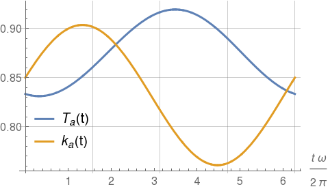
To get a first qualitative picture it is useful to set the protocols to simple sinusoidal functions (with same relative amplitude):

$$k(t) =k_{0}+\epsilon_{k}\sin(\omega t)$$ (35)

$$T(t) =T_{c}+\epsilon_{T}\frac{1-\cos(\omega t)}{2}.$$ (36)

Figure 1: A sketch of the stiffness and temperature protocols used in Section IV.A. In Section IV.B we consider a phase shift (denoted with $\phi$) with respect to the case shown in the figure, for $T(t)$, which can be adjusted to optimise the delivered power. In this plot we have chosen $T_{c}=k_{0}=1$ and $\epsilon_{k}=\epsilon_{T}=0.1$

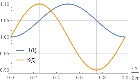
The protocol is illustrated in Fig. 1. The stiffness and temperature variations are out of phase by a fourth of a period: the temperature maximum is synchronised with the instant where the expansion (decreasing stiffness) is fastest. This choice is inspired by the classical idealised Stirling engine. In the discussion of the linear response regime, below, we show that this choice is not optimal (i.e. a slightly different lag between temperature and stiffness can be found to increase delivered power), a fact rarely discussed.

Figure 2: Study of the passive engine. A: work per cycle $W_{p}$ in the case at $\epsilon_{T}=0.1$ (blue curve, constant $T(t)=T_{c}$) and in the case $\epsilon_{T}=0.1$ (yellow curve, variable temperature). B and C: the Clapeyron plane and the different senses of rotation for two different frequencies of the engine cycle: $\omega=0.2$ (B) and $\omega=2$ (C). Parameters: in all plots $k_{0}=1$, $\epsilon_{k}=0.1$ and $T_{c}=1$.

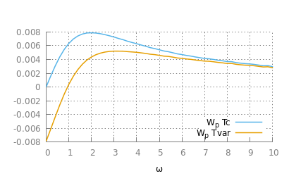
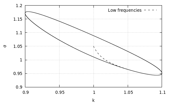
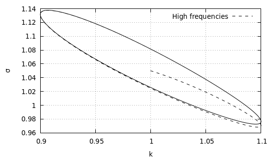
In Figure 2 we summarise the behaviour of the passive heat engine with protocol given by Eqs. (35). Frame A shows the total work per cycle $W_{p}$ as a function of $\omega$ for $\epsilon_{k}=0.1$ (with $k_{0}=1$ and $T_{c}=1$). The blue curve is for $\epsilon_{T}=0$ i.e. when the temperature does not change during the cycle (it is constant at $T=T_{c}$): the work in a period is never negative, a fact which is consistent with expectation from thermodynamics, i.e. there is no way to extract work from a single thermostat. Moreover, in the quasi-static limit $\omega\to 0$ one has $\sigma(t)=T/k(t)$ at each time. In this limit one gets $W_{p}=0$ because the curve in the $k,\sigma$ plane goes back and forth along the same route and the enclosed area is empty. As soon as a temperature variation is introduced, as seen in the yellow curve computed for $\epsilon_{T}=0.1$, the work may become negative i.e. there can be a positive power output so that the system behaves as a heat engine. This occurs at small frequencies (including the limit $\omega\to 0$), while at high frequency the work comes back to be positive and the machine stops acting as an engine. In frames B and C we show what happens in the plane $k,\sigma$. It is seen directly from Eq. (14) that a negative (= produced) work occurs when the limit cycle in that plane is swept in anti-clockwise direction, as it is observed for low frequencies (frame B) and opposite to high frequencies (frame C).

The facts observed above can be understood analytically in the small perturbation limit, computing an approximated expression for $\sigma(t)$, even before going to the full linear response treatment discussed in the next section. For this purpose we consider two simplified situations: 1) a situation where only the stiffness is perturbed so that $\epsilon_{k}=k_{0}\epsilon$ and $\epsilon_{T}=0$; 2) a situation where we assume that the two perturbations (stiffness and temperature) are similar, more precisely we set $\epsilon_{k}=k_{0}\epsilon$ and $\epsilon_{T}=\epsilon T_{c}$. In both cases we set $\sigma(t)=\sigma_{0}(t)+\epsilon\sigma_{1}(t)$ and then replace it in the expanded Eq. (17), equating equal powers in $\epsilon$, concluding by dropping terms with powers of $\epsilon$ larger than $1$.

In the first situation ($\epsilon_{k}=k_{0}\epsilon$ and $\epsilon_{T}=0$) we get

$$\frac{\sigma}{\sigma_{s}}=1+\epsilon\frac{2k_{0}}{\omega^{2}+4k_{0}^{2}}\left[-2k_{0}\sin(\omega t)+\omega\cos(\omega t)\right]$$ (37)

where we have defined the static variance $\sigma_{s}=T_{c}/k_{0}$ (the formula given here are valid if $0<\sigma_{s}<\infty$). Power adsorbed in this case reads

$$P=\epsilon^{2}k_{0}T_{c}\frac{\omega^{2}}{2(4k_{0}^{2}+\omega^{2})},$$ (38)

which is always non-negative, meaning that with $\epsilon_{T}=0$ this machine cannot do useful work, but only adsorb it.

In the second situation ($\epsilon_{k}=k_{0}\epsilon$ and $\epsilon_{T}=\epsilon T_{c}$), instead, we get:

$$\frac{\sigma}{\sigma_{s}}=1+\epsilon\left\{\frac{1}{2}+\right.\\ \left.k_{0}\;\frac{2(\omega-k_{0})\cos(\omega t)-(4k_{0}+\omega)\sin(\omega t)}{\omega^{2}+4k_{0}^{2}}\right\}$$ (39)

Integration of Eq. (14) with the latter approximated expression of $\sigma(t)$ gives for the average power

$$P=\frac{\omega}{2}k_{0}T_{c}\epsilon^{2}\frac{\omega-k_{0}}{\omega^{2}+4k_{0}^{2}}.$$ (40)

Such a formula is consistent with the observation of a critical frequency separating a regime (at low frequency) where the model produces work, i.e. $P<0$, and a regime (at high frequency) where it adsorbs work, i.e. $P>0$: in this small $\epsilon$ limit the critical frequency is $\omega^{*}=k_{0}$. Efficiency is more complicated to get, since it requires integrating the heat on the heat-adsorbing part of the cycle. In the next subsection we do the calculation of heat and efficiency, again in the linear regime, following a more powerful approach, i.e. recalling the study of Onsager coefficients done in Brandner et al. (2015) and discussing the possible optimisation strategies for the passive engine with the chosen protocols.

IV.2 Linear irreversible thermodynamics

In order to exploit general results obtained in Brandner et al. (2015), we consider here the following choices of the parameter time-dependence:

$$k(t) =k_{0}+\epsilon_{k}\gamma_{w}(t),$$ (41a)

$$T(t) =\frac{T_{c}T_{h}}{T_{h}-\epsilon_{T}\gamma_{q}(t)}\approx T_{c}+\epsilon_{T}\gamma_{q}(t),$$ (41b)

with the cold temperature $T_{c}$, the hot temperature $T_{h}=T_{c}+\epsilon_{T}$ and $\gamma_{w}(t),\gamma_{q}(t)$ two adimensional periodic functions with period $t_{cycle}$ oscillating the first between $+1$ and $-1$ and the second between $0$ and $1$. The new temperature protocols then oscillates with the same period between $T_{c}$ and $T_{c}+\epsilon_{T}$. With such a protocol one may easily see that the weighting function for adsorbed heat, needed in Eq. (8), according to the recipe in Eq. (10), is $w_{ads}(t)=\gamma_{q}(t)$. Here, we adopt the choice $\gamma_{w}(t)=\sin(\omega t)$ and $\gamma_{q}=\frac{1}{2}[1-\cos(\omega t+\phi)]$. With such a choice for small $\epsilon$ the protocol, for $\phi=0$ is identical to the protocol discussed in the previous section. The advantage of form (41b) is the possibility of inheriting all the results presented in Brandner et al. (2015) where the linear thermodynamics study of the same model has been discussed in wide generality.

Linear thermodynamics Callen (1985) is a framework where there are thermodynamic fluxes $J_{w}$ and $J_{q}$, proportional to power and rate of adsorbed heat respectively, and conjugate thermodynamic forces $F_{w}$ and $F_{q}$, proportional to maximal variations of stiffness and temperature ($\epsilon_{k}$ and $\epsilon_{T}$) respectively. More precisely, one sets

$$J_{w}=\frac{P}{T_{c}F_{w}}$$ (42)

$$J_{q}=\frac{Q_{h}}{t_{cycle}}$$ (43)

$$F_{w}=2\frac{\epsilon_{k}}{k_{0}}$$ (44)

$$F_{q}=\frac{1}{T_{c}}-\frac{1}{T_{c}+\epsilon_{T}}\approx\frac{\epsilon_{T}}{T_{c}^{2}}$$ (45)

for the fluxes and the forces respectively. We stress that in our definitions work and power are positive when adsorbed, so that $J_{w}$ has the same sign of $P$, which is different from the definition in Brandner et al. (2015). When forces are small, $F_{w}\ll 1$ and $F_{q}\ll 1$ it is possible to write linear relations between fluxes and forces, through the introduction of so-called Onsager coefficients $L_{\alpha\beta}$ with $\alpha$ and $\beta$ indices that take the value $w$ or $q$:

$$J_{w} =L_{ww}F_{w}+L_{wq}F_{q}+\mathcal{O}(F^{2}),$$ (46)

$$J_{q} =L_{qw}F_{w}+L_{qq}F_{q}+\mathcal{O}(F^{2}).$$ (47)

This immediately gives an expression for power, heat and efficiency:

$$P =T_{c}F_{w}(L_{ww}F_{w}+L_{wq}F_{q}),$$ (48)

$$\frac{Q_{h}}{t_{cycle}} =L_{qw}F_{w}+L_{qq}F_{q},$$ (49)

$$\eta =-\frac{T_{c}F_{w}(L_{ww}F_{w}+L_{wq}F_{q})}{L_{qw}F_{w}+L_{qq}F_{q}}$$ (50)

(the reader should remember that the machine does useful work when $P<0$ and $\eta>0$).

The coefficients are given by Eqs. (72) of Brandner et al. (2015) which we rewrite with our notation:

$$L_{\alpha\beta}=-\frac{2T_{c}^{2}\xi_{\alpha}\xi_{\beta}}{t_{cycle}}\int_{0}^{t_{cycle}}dt[ \dot{\gamma}_{\alpha}(t)\gamma_{\beta}(t)-$$ (51)

$$\dot{\gamma}_{\alpha}(t)\Gamma_{\alpha\beta}(t))]$$

$$\Gamma_{\alpha\beta}(t)=\int_{0}^{\infty}d\tau\dot{\gamma}_{\beta}(t-\tau)e^{-2k_{0}\tau}$$ (52)

$$\xi_{w}=\frac{1}{4T_{c}}\;\;\;\;\xi_{q}=-\frac{1}{2}$$ . (53)

For the present case (i.e. chosen harmonic potential and chosen temporal protocols), direct calculations give

$$L_{ww}(k_{0},\omega) =\frac{k_{0}\omega^{2}}{8(4k_{0}^{2}+\omega^{2})}$$ (54a)

$$L_{qq}(k_{0},\omega) =\frac{k_{0}\omega^{2}T_{c}^{2}}{8(4k_{0}^{2}+\omega^{2})}$$ (54b)

$$L_{wq}(k_{0},T_{c},\omega,\phi) =-\frac{k_{0}\omega T_{c}(2k_{0}\cos(\phi)+\omega\sin(\phi))}{8(4k_{0}^{2}+\omega^{2})}$$ (54c)

$$L_{qw}(k_{0},T_{c},\omega,\phi) =-L_{wq}(k_{0},T_{c},\omega,-\phi).$$ (54d)

The positivity of $L_{ww}$ confirms that, in the absence of a temperature variation, the work is always positive, i.e. it is always adsorbed. The relation between the off-diagonal coefficients $L_{wq}$ and $L_{qw}$ are consistent with reciprocity which is expected from the assumption of underlying time-reversible dynamics (when in the absence of thermodynamic forces) which here takes the form $L_{wq}[k(t),T(t)]=L_{qw}[k(-t),T(-t)]$ Brandner et al. (2015).

From the expressions (54) one gets the expressions for power, heat and efficiency as functions of the model’s parameters.

$$P =\frac{\omega\epsilon_{k}}{4k_{0}}\;\frac{2\epsilon_{k}\omega T_{c}-\epsilon_{T}k_{0}f_{+}(\phi,k_{0},\omega)}{4k_{0}^{2}+\omega^{2}}$$ (55a)

$$\frac{Q_{h}}{t_{cycle}} =\frac{\omega}{8}\;\frac{\epsilon_{T}k_{0}\omega+2\epsilon_{k}T_{c}f_{-}(\phi,k_{0},\omega)}{4k_{0}^{2}+\omega^{2}}$$ (55b)

$$\eta =2\frac{\epsilon_{k}}{k_{0}}\;\frac{-2\frac{\epsilon_{k}}{k_{0}}\omega+\frac{\epsilon_{T}}{T_{c}}f_{+}(\phi,k_{0},\omega)}{\frac{\epsilon_{T}}{T_{c}}\omega+2\frac{\epsilon_{k}}{k_{0}}f_{-}(\phi,k_{0},\omega)},$$ (55c)

where we have introduced the two phase-dependent frequencies $f_{\pm}(\phi,k_{0},\omega)=2k_{0}\cos(\phi)\pm\omega\sin(\phi)$. Note that the efficiency is always lower than the Carnot efficiency which is reached when $\omega\to 0$:

$$\eta(\omega>0)\leq\eta(\omega=0)=\frac{\epsilon_{T}}{T_{c}}\approx 1-\frac{T_{c}}{T_{h}}=\eta_{c}.$$ (56)

Power is negative (i.e. the machine produces work) only in a range of (non-negative) frequencies, at given $\phi$, defined by

$$\frac{\omega}{k_{0}}<r(\phi)=\eta_{c}\frac{2\cos(\phi)}{2\frac{\epsilon_{k}}{k_{0}}-\eta_{c}\sin(\phi)},$$ (57)

which implies that valid frequencies can be found only for ranges of $\phi$ such that $r(\phi)\geq 0$ (such ranges depend upon $\eta_{c}$ and $\epsilon_{k}/k_{0}$).

In formula (55a) we find interesting the role of $\phi$, which seems to us overlooked in the literature. At constant $\omega$ one can get relevant improvement in power or efficiency by tuning $\phi$: it is sufficient to consider for instance that at $\phi=0$ the range of working frequencies is $\omega<k_{0}\eta_{c}\frac{k_{0}}{\epsilon_{k}}$, but in general such a range extends to higher frequencies when $\phi$ is increased.

In conclusion we also report the expressions for power and efficiencies for the case of proportional thermodynamic forces, i.e. $\epsilon_{T}/T_{c}=\epsilon_{k}/k_{0}=\epsilon$:

$$P =\frac{\omega\epsilon^{2}k_{0}T_{c}}{4}\;\frac{2\omega-f_{+}(\phi,k_{0},\omega)}{4k_{0}^{2}+\omega^{2}}$$ (58a)

$$\eta =2\epsilon\;\frac{-2\omega+f_{+}(\phi,k_{0},\omega)}{\omega+2f_{-}(\phi,k_{0},\omega)}$$ (58b)

We note that power for $\phi=0$ has the same expression as in (40).

IV.3 Optimization of power

In Fig. 3 we show the surface $-P$ as function of $\omega,\phi$, with given $k_{0}=T_{c}=1$ and $\epsilon_{T}=\epsilon_{k}=0.1$.

Figure 3: Delivered power $-P$ as function of $\omega$ and $\phi$, with $k_{0}=T_{c}=1$ and $\epsilon_{T}=\epsilon_{k}=0.1$.

.

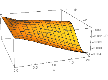
As a general feature, the surface has a positive part in the low $\omega$ and low $|\phi|$ region.

Now we find the optimal phase and frequency to get the maximum delivered power $-P$ at given $\epsilon_{T}$, $\epsilon_{k}$, $k_{0}$ and $T_{c}$. This maximum is obtained by imposing the simultaneous condition $\partial_{\phi}P=0$ and $\partial_{\omega}P=0$, and excluding solutions with $\omega\leq 0$. The result of the procedure is the following formula for the optimal values $\omega^{*}$ and $\phi^{*}$ and the corresponding values of power and efficiency:

$$\omega^{*} =2k_{0}\frac{\epsilon_{T}k_{0}}{\sqrt{(4\epsilon_{k}T_{c})^{2}-(\epsilon_{T}k_{0})^{2}}}$$ (59a)

$$\phi^{*} =\arctan\left(\frac{\omega^{*}}{2k_{0}}\right)$$ (59b)

$$-P(\phi^{*},\omega^{*}) =\frac{k_{0}\epsilon_{T}^{2}}{32T_{c}}$$ (59c)

$$\eta(\phi^{*},\omega^{*}) =\frac{\epsilon_{T}}{2T_{c}}\approx 1-\sqrt{\frac{T_{c}}{T_{h}}}$$ (59d)

Several comments are in order after looking at those formula. First of all we notice that the optimal frequency exists only if $\epsilon_{T}/T_{c}<4\epsilon_{k}/k_{0}$. Second, we confirm the interesting role of $\phi$ which must be tuned consistently to achieve maximum power. Finally we underline that the efficiency at maximum power is given by the Curzon-Ahlborn formula (approximated for small $\epsilon_{T}$) Curzon and Ahlborn (1975).

V The active heat engine

In this Section we analyze how the previous results obtained for the passive engine model can be exploited to get an optimal active heat engine. In the first subsection - for the purpose of a knowledge of all possibilities - we discuss what can be done using the dynamical UCNA approximation (small $\tau_{a}$) elaborated in Section III.3 (and frequently used in the literature for problems with constant parameters): such an approximation is useful to get a first idea of when an active machine can do useful work, however it is not obvious how it can be optimized. In the second subsection on the contrary we discuss the result of the exact equivalence between the active model and a passive one, with temperature obeying Eq. (23), exploiting the optimisation strategies of the passive model.

V.1 The small $\tau_{a}$ limit and the role of the active temperature in the dynamical UCNA approximation

As discussed in Section III.3 the dynamical UCNA approximation obtained in a weak active regime ($\tau_{a}\to 0$) constitutes an alternative mapping of an active AOUP system into a passive one, with respectively active stiffness $k_{a}(t)$ and temperature $T_{a}(t)$ given by Eqs. (30). The fact that, in the dynamical UCNA approximation, the active temperature is spontaneously time-dependent even when the characteristic energy, dictated by the active speed, $v_{0}^{2}$ is constant, leads us to argue that it is in principle possible that a thermic machine is at work by modulating in time $k(t)$ only: this would be a remarkable results, in view of the fact that for passive particles it is forbidden (see Sec. IV.A) and that it would be a great advantage for experiments, where modulating $v_{0}$ in time can be complicate.

To test this hypothesis we plug our simple protocol $k(t)$ (Eq. (35)) in the equation for the variance, obtaining $T_{a}(t)$. Then, similarly to what we did with the passive heat engine, we look for a formal solution of $\sigma(t)$ (by replacing $k$ with $k_{a}$, $T$ with $T_{a}$ in expression (34)). Given the difficulty to write explicitly this form, we move, as usual, to the linear response regime and to a numerical approach.

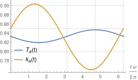
The numerical integration betrays our expectations showing that work in a cycle is positive at any frequency $\omega$ (Fig. 4)A. This is furthermore verified by the small perturbation in $\epsilon$. We proceed as in Section IV.1, expanding $\sigma(t)=\sigma_{0}(t)+\epsilon\sigma_{1}(t)$, and computing an approximated expression for $k_{a}$ and $T_{a}$ to be inserted in (17).

$$k_{a} =\frac{k_{0}}{\Gamma_{0}}+\epsilon\frac{k_{0}}{\Gamma_{0}^{2}}[\Gamma_{0}\omega\tau_{a}\cos(\omega t)+\sin(\omega t)]$$ (60a)

$$T_{a} =\frac{v_{0}^{2}\tau_{a}}{\Gamma_{0}^{2}}\bigg{[}1-\epsilon\frac{2\tau_{a}k_{0}}{\Gamma_{0}}\sin(\omega t)\bigg{]}$$ (60b)

We have used $\Gamma_{0}=1+\tau_{a}k_{0}$.

Figure 4: Study of thermodynamics for the AOUP model at small $\tau$. A: work per cycle $W_{p}$ as a function of $\omega$ in the case of constant self-propulsion speed $v_{0}$: no work is produced for $\tau_{a}=0.01$ (higher curve)$-0.1$ (lower curve). B: Active stiffness and temperature (in the case with $\tau_{a}=0.1,\omega=1$) when $v_{0}^{2}\tau_{a}=1$ is constant: maxima of $T_{a}(t)$ are always in phase with minima of $k_{a}(t)$, failing to meet a working machine condition. C: Work $W_{p}$ and adsorbed heat $Q_{h}$ per cycle when $v_{0}(t)$ is time-dependent. D: Active stiffness and temperature (with $\tau_{a}=0.2,\omega=1$) in the time-dependent $v_{0}(t)$ case. The time modulation of $v_{0}$ in C,D occurs with parameters $\tau_{a}u^{2}=1,\epsilon_{u}=0.1u^{2}$. In all plots $k_{0}=1$ and $\epsilon_{k}=0.1$.

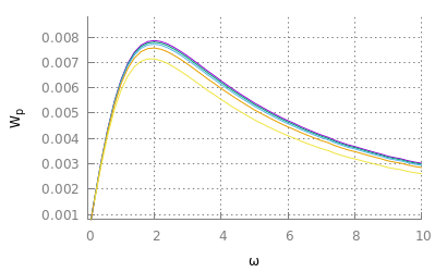
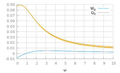
The related work $W_{p}=\epsilon^{2}(v_{0}^{2}\tau_{a})\frac{k_{0}}{2\Gamma_{0}}\>\>\frac{\omega^{2}}{4k_{0}^{2}+(\Gamma_{0}\omega)^{2}}$ is positive and does not cross 0 for any frequency value $\omega>0$. Note that in the passive limit we recover the expression for the power (38).

The fact that the pure modulation of $k(t)$, i.e. keeping $v_{0}$ constant, does not produce a working machine in the small $\tau$ limit, can be understood on a more general ground, i.e. independently of the small $\epsilon$ limit and of the choice of the protocol $k(t)$. In fact, following the qualitative discussion given in section IV, we suggest that the form of $T_{a}(t)$ with $v_{0}$ constant does not meet the requirement of a working Stirling engine: the expansions ($\dot{k}_{a}<0$) are not in phase with the maximum temperature $T_{a}$ (See Fig. 4B as an example). Given the positivity of $k$, it is straigthforward to see that the following constraints are never satisfied at the same time:

$$\begin{cases}\dot{T}_{a}=0\quad\ ;\quad\ \ddot{T}_{a}>0\\ \dot{k}_{a}<0\end{cases}$$ (61)

The presence of a lag between stiffness and temperature, such that the temperature maximum is in the expansion phase of the confining potential is decisive in the realisation of a working engine, similarly to the passive case. We need to let $v_{0}(t)$ vary in time, in order to force $T_{a}(t)$ to take the required form.

For small $\tau_{a}$ note that $k_{a}\to k$ and $T_{a}\to T_{D}=v_{0}^{2}\tau_{a}$, so it is natural to propose a $v_{0}$ which resembles the passive temperature in  (35). We take

$$v_{0}^{2}(t)=u^{2}+{\epsilon_{u}}\frac{1-\cos(\omega t)}{2}$$ (62)

This intuition is qualitatively right: the active AOUP model with a time-dependent typical velocity is able to produce work, as we can see in Fig. 4C. Along with the numerical result, it is possible to repeat our linearization strategy for $\sigma(t)$ and show that the power, obtained with the correct approximation for $T_{a}$, is $P=\epsilon^{2}(v_{0}^{2}\tau_{a})\frac{k_{0}}{2\Gamma_{0}}\>\>\frac{\omega(\omega-k_{0})}{4k_{0}^{2}+(\Gamma_{0}\omega)^{2}}$. We stress out a regime change for $\omega=k_{0}$ and the agreement with expression  (40) in the passive limit. In order to evaluate the efficiency of this working machine, in particular its behavior with $\tau_{a}$, we resort to numerical integration of adsorbed heat and work. For adosrbed heat we use definition (10) for $w_{ads}(t)$, using $T_{D}(t)=\tau_{a}v_{0}^{2}(t)$ in place of $T(t)$. The results for efficiency are represented in Fig.5: we emphasize that it is maximum in the quasi-static and in the passive limits. The effect of self-propulsion, within this approach, seems to decrease efficiency, but this is basically due to the fact that the chosen protocol is not sensitive to $\tau_{a}$ and $k(t)$, while the real effective temperature $T_{eff}$ is. Changing $\tau$ without adapting the protocol degrades the efficiency.

Figure 5: Efficiency - rescaled by the Carnot efficiency in the passive limit, $\eta_{c}=\epsilon_{u}/u^{2}=0.1$ - in small $\tau$ AOUP model when $v_{0}(t)$ follows protocol in Eq. (62), inspired by dynamical UCNA approximation. The efficiency decreases with activity. Parameters: $\omega=0.1,\epsilon_{k}=0.1,k_{0}=1$, $u^{2}=1/\tau_{a}$ and $\epsilon_{u}=0.1u^{2}$

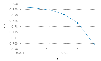
In the next section we explore the aforementioned passive-active equivalence, which gives the possibility to adjust the protocol when $\tau_{a}$ is varied, in order to control power and efficiency of the engine.

V.2 Optimisation by passive equivalence

The idea of exploiting passive-active equivalence is the following. Whatever is the particular optimisation procedure applied to the passive model, one gets optimal passive protocols $k^{*}(t)$ and $T^{*}(t)$. At that point the ”mapping equation”, Eq. (23), can be used to derive the corresponding protocols for the active models: such protocols will give exactly the same power and the same efficiency and therefore will be optimal in that particular protocols’ set. Note that, if the passive engine is optimised in the family of protocols $k(t),T(t)$ given by Equations (41a), with parameters $k_{0},T_{c},\epsilon_{k},\epsilon_{T},\omega,\phi$, the family of protocols which is spanned in the optimisation procedure is given by the same $k(t)$ and a function $v_{0}(t)$ which satisfies Eq. (23) with $T_{eff}=T(t)$. Putting Eqs. (41a) into Eq. (23), we get the corresponding family of protocols for $v_{0}(t)$

$$v_{0}^{2}(t)\tau_{a}=T(t)+\tau_{a}k(t)T(t)+$$ (63a)

$$\frac{3}{4}\omega\tau_{a}\epsilon_{T}\sin(\omega t+\phi)+$$ (63b)

$$\frac{\omega\tau_{a}^{2}}{2}\left[\epsilon_{k}\cos(\omega t)T(t)+\frac{\epsilon_{T}}{2}\sin(\omega t+\phi)k(t)\right]+$$ (63c)

$$\frac{\omega^{2}\tau_{a}^{2}\epsilon_{T}}{4}\cos(\omega t+\phi),$$ (63d)

which is parametrized by $k_{0},T_{c},\epsilon_{k},\epsilon_{T},\omega,\phi$ and also $\tau_{a}$.

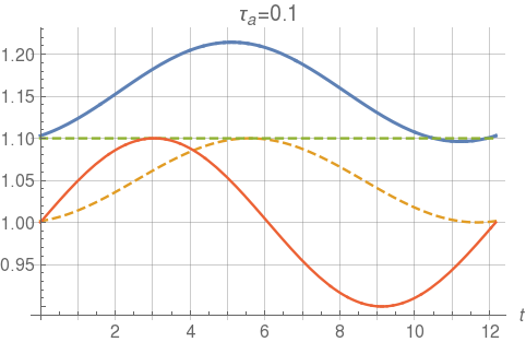
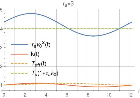
Summing up, if $\tau_{a}$ and $k(t)$ are imposed by the experiment, and one looks for an optimal $v_{0}(t)$, the task is relatively easy, i.e. one may 1) choose arbitrary values for $T_{c}$ and small $\epsilon_{T}$ (see below) and then 2) directly find the optimal $\omega^{*}$ and $\phi^{*}$ for the passive problem (in the family of sinusoidal passive protocols given by Eqs. (41a)), i.e. formula in Eqs. (59) and finally 3) use formula (63), to get the corresponding active optimal protocol for $v_{0}(t)$ which guarantees the maximum possible power and a corresponding Curzon-Ahlborn efficiency, whatever is the value of $\tau_{a}$. Given that $\epsilon_{T}/T_{c}$ must be small and therefore it is not really a free number (reasonable values are $0.1$ or smaller), some freedom remains in choosing $T_{c}$, which can be exploited in two ways: 1) one may set the desired optimal frequency $\omega^{*}$ (based upon possible experimental requirements) and then invert equation (59a) to get the corresponding $T_{c}$ or, in alternative, 2) observe that Eq. (23) is invariant for common rescaling of $T_{eff}$ (and therefore $T_{c}$) and $v_{0}^{2}$, that is one may meet any experimental upper or lower limit for $v_{0}^{2}$ by accordingly rescaling $T_{c}$.

In Figure 6 we show the optimal protocols for a given choice of $T_{c},k_{0},\epsilon_{T},\epsilon_{k}$. As anticipated, there is an important difference between the optimal protocol for $\tau_{a}v_{0}^{2}(t)$ and $T_{eff}(t)$. We underline that, following this strategy, if one spans a range of $\tau_{a}$ - keeping the same $k(t)$ - the optimal effective temperature $T_{eff}(t)$ is not changed: what is changed is the corresponding protocol for $v_{0}(t)$; if one follows it, whatever is the value of $\tau_{a}$, the power and the efficiency of the engine will always be the same. Also for this reason it is useless to show a plot with efficiencies as a function of $\tau_{a}$. The constancy of power and efficiency as a function of $\tau_{a}$ already demonstrates the superiority of this approach with respect to other approaches not informed with the correct formula for $T_{eff}$ (for instance the one of previous Section, where the efficiency decays with $\tau_{a}$, see Figure 5).

The situation is more complicate if $\tau_{a}$ and $v_{0}(t)$ are imposed by the experiment and one wants to look for the optimal $k(t)$. In such a case, a possible strategy is to use Eq. (23) to get a functional constraint between $k(t)$ and $T_{eff}(t)$; thereafter, one needs to solve the passive problem with a variation of the coupled protocols $k(t),T_{eff}(t)$ with the given constraint.

Strategies of passive-to-active equivalence are substantially simplified if very slow transformations are considered, i.e. in the limit of large period $t_{cycle}$, more precisely by taking $\tau_{a}/t_{cycle}\ll 1$. In this limit Eq. (23) is considerably simpler, as it reduces to the identity (valid for any magnitude of forces $\epsilon_{k}$ and $\epsilon_{T}$)

$$T_{eff}(t)=\frac{\tau_{a}v_{0}^{2}(t)}{1+k(t)\tau_{a}}.$$ (64)

As mentioned, in this limit $T_{eff}(t)$ is still different from $T_{a}(t)$, even at first order in $\tau_{a}$, see Eq. (31a). We underline that the same problem discussed above (see discussion above Eqs. (61)) occurs for the expression of $T_{eff}(t)$ in formula (64): if $v_{0}(t)$ is taken constant, the resulting effective temperature is always in opposition of phase with $k(t)$ (ie. maxima of $k$ correspond to minima of $T_{eff}$ and viceversa). Several empirical attempts, by numerical integration of $W_{p}$ for a wide range of choices of all the parameters convinced us that such a situation always leads to $W_{p}\geq 0$ ie. a machine that does not produce work. We recall that this is rigorously proven in the linear forcing regime (see Section IV.B and formula (55a), the opposition of phase between $k(t)$ and $T(t)$ corresponds to $\phi=-\pi/2$).

Equation (64) gives an extimate of the maximum efficiency (to be attained in the $\omega\to 0$ limit, that is at vanishing power), i.e.

$$\eta_{c}=1-\min\left\{\frac{v_{0}^{2}(t)}{1+\tau_{a}k(t)}\right\}\max\left\{\frac{v_{0}^{2}(t)}{1+\tau_{a}k(t)}\right\}^{-1}$$ (65)

which is a striking evidence of the non-trivial relation between the two thermodynamic forces (for temperature and volume forces) in shaping the efficiency of active heat engines.

Figure 6: Examples of the optimal protocol $\tau_{a}v_{0}^{2}(t)$ for an active engine to achieve maximum power when $k_{0}=T_{c}=1$ and $\epsilon_{T}=\epsilon_{k}=0.1$ (which, according to formula (59), give $\omega^{*}\approx 0.52$ and $\phi^{*}\approx 0.25$) and $\tau_{a}=0.1$. Two values are considered: $\tau_{a}=0.1$ and $\tau_{a}=3$. We underline that in both cases the engine gives the same maximum power $\approx 3\;10^{-4}$ and the same Curzon-Ahlborn efficiency $\approx 0.05$. The blue curve is $\tau_{a}v_{0}^{2}(t)$ and the red curve is $k(t)$. For reference we also put $T(t)=T_{eff}(t)=T_{c}+\epsilon_{T}\frac{1}{2}[1-\cos(\omega^{*}t+\phi^{*})]$ (yellow dashed curve), and the constant $T_{c}(1+\tau_{a}k_{0})$ (green dashed curve) which is the approximation of Eq. (63) at $0$ order in $\omega,\epsilon_{k},\epsilon_{T}$.

Equation (64) can be also used to find the shape of $v_{0}(t)$ to get any desired efficiency $\eta_{c}$ (at vanishing power, $\omega\to 0$). This is achieved by imposing that $\eta_{c}=\epsilon_{T}/(T_{c}+\epsilon_{T})$ and recalling the non-linear expression for $T(t)$, see (41b). Then we obtain

$$v_{0}^{2}(t)=\frac{T_{c}}{\tau_{a}}\frac{1+\tau_{a}k(t)}{1-\eta_{c}\gamma_{q}(t)}\xrightarrow{\tau_{a}\rightarrow\infty}\frac{T_{c}k(t)}{1-\eta_{c}\gamma_{q}(t)}.$$ (66)

We warn, however, that Eq. (64) only guarantees that the passive model with temperature $T_{eff}(t)$ gives the same evolution for $\sigma(t)$ and therefore produces/adsorbs the same work, but is not necessarily a heat engine. The positivity of work production (which in our notation corresponds to $W_{p}<0$) depends upon the phase shift between $T_{eff}(t)$ and $k(t)$. Therefore, in Eq. (66) one needs to put the proper $k(t)$ and $\gamma_{q}(t)$, i.e. the correct choices of $\omega$, $k_{0}$ and $\phi$ : the desired efficiency is reached, provided that the machine does useful work. We know however that, for small $\epsilon_{k}$ and $\epsilon_{T}$ (as demonstrated by Eq. (58a) in the $\omega\to 0$ limit), such a condition is satisfied for $\phi\in(-\pi/2,\pi/2)$.

VI Conclusions

A well defined thermostat temperature is a crucial ingredient for definitions of basic thermodynamic tools (e.g. adsorbed heat and efficiency) as well as to transfer known results valid for thermal systems: for the lack of such a well defined temperature, active heat engines elude intuition and expectation in stochastic thermodynamics. Here, building upon an important observation made in Holubec et al. (2020), we have shown an example where such a temperature can be defined and gives important advantages, useful also in experiments.

The effective temperature for this particular model satisfies Eq. (23) and is different from all other temperatures based upon particular - usually static - configurations (e.g. $T_{D}$ related to unconfined diffusion, $T_{var}$ related to equilibrium steady states, $T_{a}$ related to the small $\tau_{a}$ limit, etc.). It represents, exactly, the thermostat of an equivalent passive model which gives - in the presence of the same external harmonic potential - the same position variance and therefore the same power and the same total heat exchanged. An observation about the most correct definition of adsorbed heat (see discussion at the end of Section II) suggests that the equivalence noted in Holubec et al. (2020) cannot be extended to efficiency. Strictly speaking, efficiency of a model without a temperature is not defined at all because it is not evident how to discriminate, properly, between heat adsorbed and heat dissipated. We have bypassed this conceptual point, by considering the efficiency of the equivalent passive model. Since it is designed to give Carnot efficiency in the quasi-static limit, whatever the values of other parameters, one can use it as a proper figure of merit for the purpose of evaluating the performance of the machine.

The active-passive equivalence, Eq. (23), which contains time-derivatives of $T(t)$ and $k(t)$, suggests to study the optimisation of a passive model with smooth protocols, that is different from what usually done with piecewise linear modulations (for Carnot-like or Stirling-like engines). Therefore we have extended previous studies to a family of smooth protocols where the lag (between temperature and stiffness modulation) is varied to improve efficiency. In the linear approximation of fluxes we have found the optimal frequency and phase lag (Eqs. (59a)-(59b)) that produces maximum power output (and correspondingly Curzon-Ahlborn efficiency, roughly half of Carnot efficiency), a result which is readily translated to active engines through Eq. (23). This equivalence equation also immediately gives the Carnot efficiency of an active engine, see Eq. (65), which is valid for any activity time $\tau_{a}$ (i.e. also far from the passive limit) and any amplitude of the protocols (i.e. also far from the linear regime), but of course can be attained only in the quasi-static limit, that is at vanishing power.

Future investigations concern the possibility of extending, through suitable approximations, the results of our study to non-harmonic potentials Holubec et al. (2020), as well as to other active particle models. It is also interesting to consider fluctuations of the relevant quantities, such as power or efficiency, which constitute an important ingredient of microscopic engines. Finally, a promising direction of research is to consider bunches of active particles with interactions, in order to probe the effect of collective behavior on the performance of such kinds of heat machines.