Control of COVID-19 dynamics through a fractional-order model

Abstract

We investigate, through a fractional mathematical model, the effects of physical distance on the SARS-CoV-2 virus transmission. Two controls are considered in our model for eradication of the spread of COVID-19: media education, through campaigns explaining the importance of social distancing, use of face masks, etc., towards all population, while the second one is quarantine social isolation of the exposed individuals. A general fractional order optimal control problem, and associated optimality conditions of Pontryagin type, are discussed, with the goal to minimize the number of susceptible and infected while maximizing the number of recovered. The extremals are then numerically obtained.

url]https://orcid.org/0000-0002-2427-7704

url]https://orcid.org/0000-0002-0170-5286

url]https://orcid.org/0000-0001-8641-2505

url]https://orcid.org/0000-0002-5460-3718

1 Introduction

The availability of easy-to-use precise estimation models are essential to get an insight into the effects of transferable infectious diseases. In outbreak diseases, policy makers and institutions make decisions based on forecasting models to decide on future policies and to check the efficiency of existing policies [1].

Coronaviruses are a group of viruses that can be transmitted between humans, livestock and wild animals. Person to person spread of COVID-19 happens through close contact, up to six feet. This group of viruses mainly affects the hepatic, neurological and respiratory systems [2, 3, 4].

In the end of 2019, the World Health Organization (WHO) reported a novel coronavirus in China, which causes severe damage to the respiratory system. The virus was first found in Wuhan city, and was named as severe acute respiratory syndrome coronavirus 2 (SARS-CoV-2) [5]. After the outbreak of the virus, the Chinese government put several cities on lock down [6, 7]. However, the number of affected people increased daily within China and in other countries. In March 11, 2020, COVID-19 was declared as a global pandemic by WHO. At the time we write these lines, January 6, 2021, approximately 87 million people were infected with 1.9 million of deaths, worldwide [8].

Recently, many mathematical models were proposed to understand disease transmission and project handful controls: see, e.g., [9, 10, 11] and references therein. Simultaneously, all health organizations are trying to drive the most lethal infectious diseases towards eradication, using educational and enlightenment campaigns, vaccination, treatment, etc. However, many of these infectious diseases will become eventually endemic because of interventions to mitigate the spread in time and lack of adequate policies. For control of infectious diseases, proactive steps are required, specially for diseases having vaccine and cure. Indeed, some times it is more difficult to control the spread of an infectious disease than to cure it. Regarding COVID-19, several vaccines begin to be available [12].

Optimal control theory is a branch of mathematical optimization that deals with finding a control for a dynamical system, over a period of time, such that an objective function is minimized or maximized. Along the years, optimal control theory has found applications in several fields, containing process control, aerospace, robotics, economics, bio-engineering, management sciences, finance, and medicine [13, 14, 15]. In particular, the study of epidemic models is strongly related to the study of control strategies, as screening and educational campaigns [16], vaccination [17], and resource allocation [18].

In the current pandemic situation of COVID-19, due to best presentation of memory effects and its usefulness in many different and widespread phenomena [19, 20, 21, 22, 23, 24, 25], fractional (non-integer order) models are receiving the attention of many researchers: see, e.g., [26, 27, 28, 29, 30, 31, 32, 33, 34, 35, 36, 37, 38]. Here, with the purpose to control the current pandemic, we follow two control variables, in the form of media (education) campaigns, social distance, and use of mask for protection of susceptible individuals; and quarantine (social isolation) for the exposed. For a general non-integer order optimal control problem, necessary optimality conditions are presented, with the help of Caputo derivatives. One of the great advantages of the Caputo fractional derivative is that it allows traditional initial or boundary conditions to be included in the formulation of the problem. More concretely, we minimize the number of susceptible and infected, while maximizing the number of recovered population from COVID-19. The optimal levels of the proposed two controls are characterized using the fractional version of Pontryagin’s maximum principle. The resulting optimality system is then solved numerically with Matlab.

The rest of the paper is arranged as follows. In Section 2, we present our fractional mathematical model. Section 3 recalls the fundamental definitions and the main result of fractional optimal control. We then derive an optimal control problem in Section 4, while parameter estimation with numerical results are discussed in Section 5. We finish with some remarks and conclusions, in Section 6.

2 The fractional model

Our model consists of four classes: $S(t)$, which represents the vulnerable individuals (healthy people but who may get the disease in a near future); $E(t)$, representing the exposed population or individuals who are infected but not yet infectious; the group $I(t)$, devoted to the population who are confirmed infected (individuals who have contracted the disease and are now sick with it and are infectious); the group $R(t)$, defined as the recovered population (individuals who have recovered from COVID-19). For the dynamics of this base model, see [28]. Thus, the fractional order model we consider here is given by

$$\left\{\begin{array}[]{rcl}{}_{0}^{C}D_{t}^{\alpha}S(t)&=&\Lambda-\beta_{1}S(t)E(t)-\beta_{2}S(t)I(t)-\mu S(t)+\tau R(t),\cr{}_{0}^{C}D_{t}^{\alpha}E(t)&=&\beta_{1}S(t)E(t)+\beta_{2}S(t)I(t)-(\mu+\rho)E(t),\cr{}_{0}^{C}D_{t}^{\alpha}I(t)&=&\rho E(t)-(\gamma+d+\mu)I(t),\cr{}_{0}^{C}D_{t}^{\alpha}R(t)&=&\gamma I(t)-(\mu+\tau)R(t),\end{array}\right.$$ (1)

where $\Lambda$ is the recruitment rate, $\beta_{1}$ and $\beta_{2}$ are the incidence rates, $\tau$ is the relapse rate, $\mu$ is the natural death rate, $\rho$ the rate at which the exposed population of COVID-19 join the infectious class, $\gamma$ the recovery rate of infected population, and $d$ is the death rate of infected class due to the SARS-CoV-2 virus. The total population $N(t)$ is given, at each instant of time, by

$$N(t)=S(t)+E(t)+I(t)+R(t).$$ (2)

By adding all the equations of system (1), we have

$$_{0}^{C}D_{t}^{\alpha}N(t)=\Lambda-\mu N(t)-dI(t)\leq\Lambda-\mu N(t).$$ (3)

3 Basics of fractional control theory

In this section we recall the basic definitions of Caputo fractional calculus and the central result of fractional optimal control theory [23, 39], which are required for the coming sections.

Definition 1.

For $f\in C^{m}$, $m\in\mathbb{N}$, the left-sided Caputo fractional derivative is given by

$${{}_{a}^{C}D_{t}^{\alpha}}f(t)=\frac{1}{\Gamma(m-\alpha)}\int_{a}^{t}(t-\tau)^{m-\alpha-1}\left(\frac{d}{d\tau}\right)^{m}f(\tau)d\tau,$$ (4)

while the right-sided Caputo fractional derivative is given by

$${{}_{t}^{C}D_{b}^{\alpha}}f(t)=\frac{1}{\Gamma(m-\alpha)}{\int_{t}^{b}}(\tau-t)^{m-\alpha-1}\left(-\frac{d}{d\tau}\right)^{m}f(\tau)d\tau,$$ (5)

where $\alpha$ stands for order of the derivative, $m-1<\alpha\leq m$.

Definition 2.

For $f$ an integrable function, the left-sided Riemann–Liouville fractional derivative is defined by

$${{}_{a}D_{t}}^{\alpha}f(t)=\frac{1}{\Gamma(m-\alpha)}\left(\frac{d}{dt}\right)^{m}\int_{a}^{t}(t-\tau)^{m-\alpha-1}f(\tau)d\tau,$$ (6)

while the right-sided Riemann–Liouville derivative of $f$ is given by

$${{}_{t}D_{b}^{\alpha}}f(t)=\frac{1}{\Gamma(m-\alpha)}\left(-\frac{d}{dt}\right)^{m}{\int_{t}^{b}}(\tau-t)^{m-\alpha-1}f(\tau)d\tau,$$ (7)

where $\alpha$ is the order of the derivative with $m-1<\alpha\leq m$, $m\in\mathbb{N}$.

Our control system is described by a fractional differential system (FDS) with a given/fixed initial condition as follows:

$$\begin{cases}{}_{0}^{C}D_{t}^{\alpha}X(t)=f\left(X(t),u(t),t\right),\\ X(0)=X_{0},\end{cases}$$ (8)

where $\alpha\in(0,1]$, the $n$-dimensional $X(t)$ is the state vector, $f$ is a given vector-valued function, $t\in[0,t_{f}]$ with $t_{f}>0$ the ending time of the control process, and $m$-dimensional $u(t)$ is the control vector. A fractional optimal control problem consists to minimize or maximize a performance index

$$J\left[u(\cdot)\right]=\theta\left(X(t_{f}),t_{f}\right)+\int\limits_{0}^{t_{f}}\phi\left(X(t),u(t),t\right)dt$$ (9)

subject to the control system (8) (see, e.g., [39, 40]). Functions $\theta$ and $\phi$ will be specified in Section 4. Note that here $t_{f}$ is fixed but $X(t_{f})$ is free. For finding the optimal control law $u(t)$ solution to the optimal control problem (8)–(9), we use the fractional version of Pontryagin maximum principle, which coincides with the classical Pontryagin maximum principle when $\alpha=1$:

Theorem 3 (See, e.g., [39, 40]).

For the optimality of (8)–(9), a necessary condition is given by

$$\begin{cases}\frac{\partial\phi}{\partial u}\left(X(t),u(t),t\right)+\lambda^{T}\frac{\partial f}{\partial u}\left(X(t),u(t),t\right)=0,\\ {}_{0}^{C}D_{t}^{\alpha}X(t)=f\left(X(t),u(t),\left(t\right)\right),\quad X(0)=X_{0},\\ {}_{t}D_{t_{f}}^{\alpha}\lambda(t)=\frac{\partial\phi}{\partial X}\left(X(t),u(t),t\right)+\lambda^{T}\frac{\partial f}{\partial X}\left(X(t),u(t),t\right),\quad\lambda(t_{f})=\frac{\partial\theta}{\partial X}\left(X(t_{f}),t_{f}\right).\end{cases}$$

In the next section, we compute the optimal control strategy for the fractional order COVID-19 model, which is a hot topic in current times.

4 Fractional-order model with controls

We implement an optimal control technique to the fractional order model (1). With the purpose to control the spread of the COVID-19 pandemic in the world, we use two control variables in the form of media (educational) campaigns, social distance, and use of masks — the control $u_{1}(t)$ — applied to the susceptible class; and quarantine (social isolation) — the control $u_{2}(t)$ — applied to the exposed class. Then, the new system with controls is given by

$$\begin{cases}{}_{0}^{C}D_{t}^{\alpha}S(t)=\Lambda-\beta_{1}S(t)E(t)-\beta_{2}S(t)I(t)-\mu S(t)+\tau R(t)-u_{1}(t)S(t),\cr{}_{0}^{C}D_{t}^{\alpha}E(t)=\beta_{1}S(t)E(t)+\beta_{2}S(t)I(t)-(\mu+\rho)E(t)-u_{2}(t)E(t),\cr{}_{0}^{C}D_{t}^{\alpha}I(t)=\rho E(t)-(\gamma+d+\mu)I(t)+(1-p)u_{2}(t)E(t),\cr{}_{0}^{C}D_{t}^{\alpha}R(t)=\gamma I(t)-(\mu+\tau)R(t)+u_{1}(t)S(t)+pu_{2}(t)E(t),\end{cases}$$ (10)

where the fractional order $\alpha$ is a real number in the interval $(0,1]$ and $p$ can be interpreted as the probability of infected individuals to recover by quarantine. In vector form, the system (10) can be written as

$$_{0}^{C}D_{t}^{\alpha}{X(t)}=f\left(X(t),u(t)\right),$$ (11)

where $X(t)=\left(S(t),E(t),I(t),R(t)\right)$ represents the state-vector and $u(t)=\left(u_{1}(t),u_{2}(t)\right)$ stands for the control-vector.

Our optimal control problem consists to minimize the spread of COVID-19 and maximize the number of recovered population. The following objective functional is defined with this purpose:

$$J[u(\cdot)]=A_{3}S(t_{f})+A_{4}E(t_{f})+\int_{0}^{t_{f}}A_{1}I(t)-A_{2}R(t)+\frac{1}{2}\left(r_{1}u_{1}^{2}(t)+r_{2}u_{2}^{2}(t)\right)dt\longrightarrow\min,$$ (12)

where the positive weights $A_{i}$, $i=1,2,3,4$, and $r_{i}$, $i=1,2$, are used to balance the control factors. The objective functional (12) is a particular case of the general form (9) discussed in Section 3, and can be written as

$$J[u(\cdot)]=\theta\left(X(t_{f})\right)+\int_{0}^{t_{f}}\phi\left(X(t),u(t)\right)dt$$ (13)

with $\theta\left(X(t_{f})\right)=A_{3}S(t_{f})+A_{4}E(t_{f})$ and

$$\phi\left(X(t),u(t)\right)=A_{1}I(t)-A_{2}R(t)+\frac{1}{2}\left(r_{1}u_{1}^{2}(t)+r_{2}u_{2}^{2}(t)\right).$$

Similar functionals (13) to be optimized, e.g. for optimal control problems in the combat of Zika and Ebola, have been previously considered in the literature, see [41, 42] and references therein. By using Theorem 3, the following necessary optimality conditions can be written: the control system and its initial condition,

$$\begin{cases}{}_{0}^{C}D_{t}^{\alpha}X=f\left(X,u\right),\\ X(0)=X_{0},\end{cases}$$ (14)

the adjoint system and its transversality condition,

$$\begin{cases}{}_{t}D_{t_{f}}^{\alpha}\lambda(t)=\frac{\partial\phi}{\partial X}+\lambda^{T}\frac{\partial f}{\partial X},\\ \lambda(t_{f})=\left.\frac{\partial\theta}{\partial X}\right|_{t_{f}},\end{cases}$$ (15)

and the stationary condition

$$\frac{\partial\phi}{\partial u}+\lambda^{T}\frac{\partial f}{\partial u}=0,$$ (16)

where $\lambda(t)=\left(\lambda_{1}(t),\lambda_{2}(t),\lambda_{3}(t),\lambda_{4}(t)\right)$ and $f=\left(f_{1},f_{2},f_{3},f_{4}\right)$ with

$$\begin{split}f_{1}&=\alpha-\beta_{1}S(t)E(t)-\beta_{2}S(t)I(t)-\mu S(t)+\tau R(t)-u_{1}(t)S(t),\\ f_{2}&=\beta_{1}S(t)E(t)+\beta_{2}S(t)I(t)-(\mu+\rho)E(t)-u_{2}(t)E(t),\\ f_{3}&=\rho E(t)-(\gamma+d+\mu)I(t)+(1-p)u_{2}(t)E(t),\\ f_{4}&=\gamma I(t)-(\mu+\tau)R(t)+u_{1}(t)S(t)+pu_{2}(t)E(t).\end{split}$$

The adjoint system of Pontryagin’s maximum principle asserts that

$$\begin{cases}{}_{t}D_{t_{f}}^{\alpha}\lambda_{1}(t)=-\lambda_{1}\beta_{1}E(t)-\lambda_{1}\beta_{2}I(t)-\lambda_{1}\mu+\lambda_{2}\beta_{1}E(t)+\lambda_{2}\beta_{2}I(t),\cr{}_{t}D_{t_{f}}^{\alpha}\lambda_{2}(t)=-\lambda_{1}\beta_{1}S(t)+\lambda_{2}\beta_{1}S(t)-\lambda_{2}\mu-\lambda_{2}\rho+\lambda_{3}\rho,\cr{}_{t}D_{t_{f}}^{\alpha}\lambda_{3}(t)=A_{1}-\beta_{2}\lambda_{1}S(t)+\beta_{2}\lambda_{2}S(t)-(\gamma+d+\mu)\lambda_{3}+\gamma\lambda_{4},\cr{}_{t}D_{t_{f}}^{\alpha}\lambda_{4}(t)=\tau\lambda_{1}-\lambda_{4}(\tau+\mu)-A_{2},\end{cases}$$ (17)

subject to the transversality conditions

$$\begin{cases}\lambda_{1}(t_{f})=A_{3},\cr\lambda_{2}(t_{f})=A_{4},\cr\lambda_{3}(t_{f})=0,\cr\lambda_{4}(t_{f})=0.\end{cases}$$ (18)

The optimal control variables are given by the stationary conditions:

$$\begin{cases}u_{1}(t)=\frac{(\lambda_{1}(t)-\lambda_{4}(t))S(t)}{r_{1}},\cr u_{2}(t)=\frac{(\lambda_{2}-(1-\rho)\lambda_{3}-\rho\lambda_{4})E(t)}{r_{2}}.\end{cases}$$ (19)

These analytic necessary optimality conditions are solved numerically in Section 5.

5 Numerical simulations

To illustrate the theoretical results presented in previous sections, here we use numerical simulations. For this purpose, a program was developed in Matlab to integrate the necessary optimality conditions and, with the help of a number of simulations, a detailed output is comprehensively verified. As explained in Section 4, we obtain the optimality system for the proposed optimal control problem from the state and adjoint equations subject to suitable boundary conditions: the initial conditions $X(0)=X_{0}$ on the state variables, see (14); and the terminal conditions on the adjoint variables provided by the transversality conditions, see (18). Furthermore, we obtain the optimal control strategies from the stationary system, see (19). We use a forward time/backward space finite-difference numerical method. Beginning with an initial guess for the adjoint variables, a forward time and backward space finite-difference method is used to solve the state equations. The key is to rewrite the control system (11) into the equivalent integral form

$$X(t)=X(0)+\frac{1}{\Gamma(\alpha)}{\displaystyle\int\limits_{0}^{t}}(t-\tau)^{\alpha-1}f(X(\tau),u(\tau))d\tau$$

and then use the generalized Adams-type predictor-corrector method [21, 22] for solution. Further, these state values are used for the solution of the adjoint equations by a backward time and forward space finite-difference method, because of the transversality conditions. System (15) is written, in an equivalent way, as the integral equation

$$\lambda(t)=\left.\frac{\partial\theta}{\partial X}\right|_{t_{f}}+\frac{1}{\Gamma(\alpha)}{\displaystyle\int\limits_{t}^{t_{f}}}(\tau-t)^{\alpha-1}\left[\frac{\partial\phi}{\partial X}+\lambda^{T}\frac{\partial f}{\partial X}\right]d\tau.$$

Using a steepest-method to generate a successive approximation of the optimal control form, we continue iterating until convergence is achieved. For illustrative purposes, take the initial values as $S(0)=220$, $E(0)=100$, $I(0)=3$, $R(0)=0$ and parameter values as $\Lambda=0.271$, $\beta_{1}=0.00035$, $\beta_{2}=0.00040$, $\mu=0.001$, $\rho=0.00580$, $\gamma=0.007$, $\tau=0.002$, $p=0.3$, and $d=0.00025$.

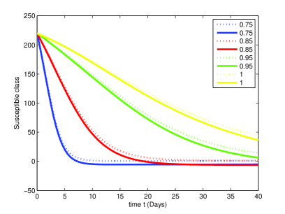
In Figure 1, we plot the susceptible population of systems (1) and (10). The doted lines denote the population of class $S$ in the uncontrolled system (1), without controls, while the solid lines denote the population of $S(t)$ in the controlled system (10), under optimal controls for $\alpha=0.75$, $0.85$, $0.95$ and $1$.

Figure 1: The susceptible population $S(t)$, with and without controls, respectively solid and doted lines, for $\alpha=0.75,0.85,0.95,1$.

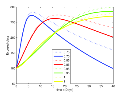
Figure 2 represents the exposed population of both systems (1) and (10). The doted lines show that there are more exposed individuals when no control measures are implemented.

Figure 2: The exposed class $E(t)$ of individuals, with and without controls, respectively solid and doted lines, for $\alpha=0.75,0.85,0.95,1$.

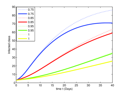
Figure 3 illustrates the infectious population $I(t)$ of system (1), without any control, and that of system (10) with controls. The doted lines make it clear that there are more infectious individuals when no control is implemented.

Figure 3: Infected population for systems with and without controls, respectively solid and doted lines, for $\alpha=0.75,0.85,0.95,1$.

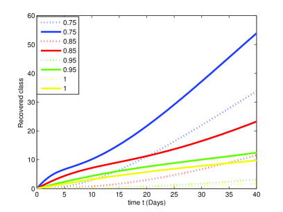
Finally, Figure 4 illustrates the recovered population $R(t)$. We see that there are more recovered individuals in the case one uses optimal control theory (because there is less susceptible, exposed and infected).

Figure 4: Recovered individuals for systems with and without controls, respectively solid and doted lines, for $\alpha=0.75,0.85,0.95,1$.

6 Conclusion

The current pandemic situation due to COVID-19 affects the whole world on an unprecedented scale. In this work, we implemented optimal control techniques to the COVID-19 pandemic through a fractional order model. For the eradication of virus spread throughout the world, we applied two controls in the form of media (education) campaigns, social distance, use of masks and protection for the susceptible class; and quarantine (social isolation) for the exposed individuals. We discussed necessary optimality conditions for a general fractional optimal control problem, whose fractional system is described in the Caputo sense while the adjoint system involves Riemann–Liouville derivatives. In the COVID-19 setting, we minimize the number of susceptible and infected population, while maximizing the number of recovered population from SARS-CoV-2 virus. Using the fractional version of Pontryagin’s maximum principle, we characterize the optimal levels of the proposed controls. The resulting optimality system is solved numerically in the Matlab numerical computing environment. Our numerical experiments were based on data of [27]. In a future work, we plan to use real data of Africa, USA and UK.

References

- [1] Chatterjee, K., Chatterjee, K., Kumar, A., & Shankar, S. (2020). Healthcare impact of COVID-19 epidemic in India: A stochastic mathematical model. Medical Journal Armed Forces India, 76(2), 147–155. https://doi.org/10.1016/j.mjafi.2020.03.022
- [2] Duan, L., & Zhu, G. (2020). Psychological interventions for people affected by the COVID-19 epidemic. The Lancet Psychiatry, 7(4), 300–302. https://doi.org/10.1016/S2215-0366(20)30073-0
- [3] Schett, G., Sticherling, M., & Neurath, M. F. (2020). COVID-19: risk for cytokine targeting in chronic inflammatory diseases? Nature Reviews Immunology, 20(5), 271–272. https://doi.org/10.1038/s41577-020-0312-7
- [4] Seah, I., & Agrawal, R. (2020). Can the coronavirus disease 2019 (COVID-19) affect the eyes? A review of coronaviruses and ocular implications in humans and animals. Ocular Immunology and Inflammation, 28(3), 391–395. https://doi.org/10.1080/09273948.2020.1738501
- [5] Lau, H., Khosrawipour, V., Kocbach, P., Mikolajczyk, A., Schubert, J., Bania, J., & Khosrawipour, T. (2020). The positive impact of lockdown in Wuhan on containing the COVID-19 outbreak in China. Journal of Travel Medicine, 27(3), taaa037. https://doi.org/10.1093/jtm/taaa037
- [6] Liang, R., Lu, Y., Qu, X., Su, Q., Li, C., Xia, S., Liu, Y., Zhang, Q., Cao, X., Chen, Q., & Niu, B. (2020) Prediction for global African swine fever outbreaks based on a combination of random forest algorithms and meteorological data. Transbound Emerg. Dis., 67, 935–946. https://doi.org/10.1111/tbed.13424
- [7] Liu, W., Zhang, Q., Chen, J., Xiang, R., Song, H., Shu, S., & You, L. (2020). Detection of Covid-19 in children in early January 2020 in Wuhan, China. New England Journal of Medicine, 382(14), 1370–1371. https://doi.org/10.1056/NEJMc2003717
- [8] Worldometer, COVID-19 Coronavirus Pandemic, Last accessed: 06-Jan-2021. https://www.worldometers.info/coronavirus
- [9] Lemos-Paião, A.P., Silva, C.J., & Torres, D.F.M. (2020) A new compartmental epidemiological model for COVID-19 with a case study of Portugal, Ecological Complexity, 44, Art. 100885, 8 pp. https://doi.org/10.1016/j.ecocom.2020.100885 arXiv:2011.08741
- [10] Ndaïrou, F., Area, I., Nieto, J.J., & Torres, D.F.M. (2020) Mathematical modeling of COVID-19 transmission dynamics with a case study of Wuhan, Chaos Solitons Fractals, 135, 109846, 6 pp. https://doi.org/10.1016/j.chaos.2020.109846 arXiv:2004.10885
- [11] Zine, H., Boukhouima, A., Lotfi, E.M., Mahrouf, M., Torres, D.F.M., & Yousfi, N. (2020) A stochastic time-delayed model for the effectiveness of Moroccan COVID-19 deconfinement strategy, Math. Model. Nat. Phenom., 15, Paper No. 50, 14 pp. https://doi.org/10.1051/mmnp/2020040 arXiv:2010.16265
- [12] The New York Times, Coronavirus Vaccine Tracker, Last accessed: 30-Nov-2020. https://www.nytimes.com/interactive/2020/science/coronavirus-vaccine-tracker.html
- [13] Kostylenko, O., Rodrigues, H.S., & Torres, D.F.M. (2019) The risk of contagion spreading and its optimal control in the economy, Stat. Optim. Inf. Comput., 7(3), 578–587. https://doi.org/10.19139/soic.v7i3.833 arXiv:1812.06975
- [14] Lemos-Paião, A.P., Silva, C.J., Torres, D.F.M., & Venturino, E. (2020) Optimal control of aquatic diseases: a case study of Yemen’s cholera outbreak, J. Optim. Theory Appl., 185(3), 1008–1030. https://doi.org/10.1007/s10957-020-01668-z arXiv:2004.07402
- [15] Sidi Ammi, M.R., & Torres, D.F.M. (2019) Optimal control of a nonlocal thermistor problem with ABC fractional time derivatives, Comput. Math. Appl., 78(5), 1507–1516. https://doi.org/10.1016/j.camwa.2019.03.043 arXiv:1903.07961
- [16] Castilho, C. (2006) Optimal control of an epidemic through educational campaigns, Electron. J. Differential Equations, 2006(125), 11 pp. https://ejde.math.txstate.edu/Volumes/2006/125/castilho.pdf
- [17] Brandeau, M.L., Zeric, G.S., & Richter, A. (2003) Resource allocation for control of infectious diseases in multiple independent populations: Beyond cost-effectiveness analysis, Journal of Health Economics 22(4), 575–598. https://doi.org/10.1016/S0167-6296(03)00043-2
- [18] Ball, F., & Becker, N. G. (2006) Control of transmission with two types of infection, Math. Biosci., 200(2), 170–187. https://doi.org/10.1016/j.mbs.2005.12.024
- [19] Anastasio, T.J. (1994) The fractional order dynamics of bainstem vestibulooculomotor neurons, Biolog. Cybern., 72, 69–79. https://doi.org/10.1007/BF00206239
- [20] Agrawal, O.P. (2004) A general formulation and solution scheme for fractional optimal control problems, Nonlinear Dyn., 38, 323–337. https://doi.org/10.1007/s11071-004-3764-6
- [21] Diethelm, K., Ford, N.J., & Freed, A.D. (2002) A predictor-corrector approach for the numerical solution of fractional differential equations, Nonlinear Dyn., 29, 3–22. https://doi.org/10.1023/A:1016592219341
- [22] Diethelm, K. , Ford, N.J., & Freed, A.D. (2004), Detailed error analysis for a fractional Adams method, Numer. Algo., 36(1), 31–52. https://doi.org/10.1023/B:NUMA.0000027736.85078.be
- [23] Agrawal, O.P. (2008) A quadratic numerical scheme for fractional optimal control problems, J. Dyn. Syst. Meas. Control, 130(1), 1–6. https://doi.org/10.1115/1.2814055
- [24] Tricaud, C., & Chen, Y. (2010) An approximation method for numerically solving fractional order control problems of general form, Comput. Math. Appl., 59(5), 1644–1655. https://doi.org/10.1016/j.camwa.2009.08.006
- [25] Biswas, R.K., & Sen, S. (2011) Fractional optimal control problems with specified final time, J. Comput. Non. Dyn., 6(2), 021009, 6 pp. https://doi.org/10.1115/1.4002508
- [26] Ali, S.A., Baloch, M., Ahmed, N., Ali, A.A., & Iqbal, A. (2020) The outbreak of coronavirus disease 2019 (COVID-19)—An emerging global health threat, Journal of Infection and Public Health., 13(4), 644–646. https://doi.org/10.1016/j.jiph.2020.02.033
- [27] Ndaïrou, F., Area, I., Nieto, J.J., Silva, C.J., & Torres, D.F.M. (2021) Fractional model of COVID-19 applied to Galicia, Spain and Portugal, Chaos Solitons Fractals 144 (2021), Art. 110652, 7 pp. https://doi.org/10.1016/j.chaos.2021.110652 arXiv:2101.01287
- [28] Zhang, Z. (2020) A novel COVID-19 mathematical model with fractional derivatives: Singular and nonsingular kernels, Chaos Solitons Fractals, 139, 110060, https://doi.org/10.1016/j.chaos.2020.110060
- [29] Zeb, A., Alzahrani, E., Erturk, V.S., & Zaman, G. (2020) Mathematical model for coronavirus disease 2019 (COVID-19) containing isolation class, BioMed Research International, Article ID 3452402, 7 pp. https://doi.org/10.1155/2020/3452402
- [30] Yousaf, M., Muhammad, S.Z., Muhammad, R.S., & Shah, H.K. (2020) Statistical analysis of forecasting COVID-19 for upcoming month in Pakistan, Chaos, Solitons & Fractals, 138, 109926. https://doi.org/10.1016/j.chaos.2020.109926
- [31] Shah, K., Abdeljawad, T., Mahariq, I., & Jarad, F. (2020) Qualitative analysis of a mathematical model in the time of COVID-19, 2020, ID 5098598, 11 pp. https://doi.org/10.1155/2020/5098598
- [32] Din, R.U., Shah, K., Ahmad, I., & Abdeljawad, T. (2020) Study of transmission dynamics of novel COVID-19 by using mathematical model, Advances in Difference Equations, 2020(323), https://doi.org/10.1186/s13662-020-02783-x
- [33] Zhang, Z., Zeb, A., Egbelowo, O.F., & Erturk, V.S. (2020) Dynamics of a fractional order mathematical model for COVID-19 epidemic, Advances in Difference Equations, 2020, Art. 420, 16 pp. https://doi.org/10.1186/s13662-020-02873-w
- [34] Zhang, Z., Zeb, A., Hussain, S., & Alzahrani, E. (2020) Dynamics of COVID-19 mathematical model with stochastic perturbation, Advances in Difference Equations, 2020, Art. 451, 12 pp. https://doi.org/10.1186/s13662-020-02909-1
- [35] Atangana, A. (2018) Blind in a commutative world: Simple illustrations with functions and chaotic attractors, Chaos, Solitons & Fractals, 114, 347–363. https://doi.org/10.1016/j.chaos.2018.07.022
- [36] Atangana, A. (2020) Fractional discretization: The African’s tortoise walk, Chaos, Solitons & Fractals, 130, 109399. https://doi.org/10.1016/j.chaos.2019.109399
- [37] Atangana, A. (2017) Fractal-fractional differentiation and integration: Connecting fractal calculus and fractional calculus to predict complex system, Chaos, Solitons & Fractals, 102, 396–406. https://doi.org/10.1016/j.chaos.2017.04.027
- [38] Ghanbari, B., & Atangana, A. (2020) Some new edge detecting techniques based on fractional derivatives with non-local and non-singular kernels, Advances in Difference Equations, 2020, Article 435, 19 pp. https://doi.org/10.1186/s13662-020-02890-9
- [39] Agarwal, R.P., Baleanu, D., Nieto, J.J., Torres, D.F.M., & Zhou, Y. (2018) A survey on fuzzy fractional differential and optimal control nonlocal evolution equations, J. Comput. Appl. Math., 339, 3–29. https://doi.org/10.1016/j.cam.2017.09.039 arXiv:1709.07766
- [40] Almeida, R., Pooseh, S., & Torres, D.F.M. (2015) Computational methods in the fractional calculus of variations, Imperial College Press, London. https://doi.org/10.1142/p991
- [41] Ndaïrou, F., Area, I., Nieto, J. J., Silva, C. J., & Torres, D.F.M. (2018) Mathematical modeling of Zika disease in pregnant women and newborns with microcephaly in Brazil, Math. Methods Appl. Sci., 41(18), 8929–8941. https://doi.org/10.1002/mma.4702 arXiv:1711.05630
- [42] Area, I., Ndaïrou, F., Nieto, J. J., Silva, C. J., & Torres, D.F.M. (2018) Ebola Model and Optimal Control with Vaccination Constraints, J. Ind. Manag. Optim. 14 (2018), no. 2, 427–446. https://doi.org/10.3934/jimo.2017054 arXiv:1703.01368