Quasiparticle Pattern of Phenomena in Exotic Superconductors

Abstract

The quasiparticle formalism invented by Lev Landau for description of conventional Fermi liquids is generalized to exotic superconductivity attributed to Cooper pairing, whose measured properties defy explanation within the standard BCS-Fermi Liquid description. We demonstrate that in such systems the quasiparticle number remains equal to particle number, just as in common Fermi liquids. We are then able to explain the puzzling relationship between the variation with doping $x$ of two key properties of the family La_2-xSr_xCu0₄ of exotic superconductors, namely the $T=0$ superfluid density $\rho_{s0}(x)$ and the coefficient $A_{1}(x)$ in the linear-in-$T$ component of the normal-state low-$T$ resistivity $\rho(T)=\rho_{0}+A_{1}T+A_{2}T^{2}$, in terms of the presence of interaction-induced flat bands in the ground states of these metals.

The BCS paradigm BCS ; gor'kov ; eliash , emergent more than half a century ago, has successfully explained the phenomenon of superconductivity discovered by Kamerlingh Onnes in 1911. This success rests upon (i) the Cooper scenario for electron pairing in metals cooper and (ii) the Landau quasiparticle formalism, applicable to the normal state of a Fermi liquid (FL) provided the damping $\gamma$ of single-particle excitations is small compared with their energy $\epsilon({\bf p})$ measured from the chemical potential $\mu$ lan1 ; lan2 . Subsequently, Larkin and Migdal (LM) adapted the BCS-FL theory to quantitative description of superfluid liquid ³He LM ; migdal . One of the prominent LM results is that the $T=0$ superfluid density $\rho_{s0}$ coincides with total density $\rho$, irrespective of the strength of interparticle forces.

However, the LM theory fails to describe superconducting alloys. In the presence of impurity-induced electron scattering, the damping $\gamma$ becomes finite, rendering the Landau postulate $\gamma/|\epsilon({\bf p})|\ll 1$ inapplicable. In the analysis of the properties of these metals pioneered by Abrikosov and Gor’kov(AG) AG , an additional dimensionless parameter $\gamma/T_{c}(x)$ comes into play, resulting in substantial suppression of $\rho_{s0}$ as observed experimentally, with $\rho_{s0}(x)$ coming to naught at a doping value $x_{c}$, in tandem with the critical temperature $T_{c}(x)$. Although the effects of $e-e$ interaction are ignored in AG theory, their involvement within the standard BCS-FL approach makes little difference prb2019 . These findings suggest that the replacement of FL quasiparticles by more realistic quasiparticles of finite lifetime is instrumental to elucidating the properties of superconducting alloys.

The BCS-FL-AG era ended dramatically with the discovery by Bednorz and Müller (BM) BM of exotic superconductivity, whose properties defy explanation within the BCS paradigm, opening up a new chapter of condensed-matter physics devoted to studies of non-Fermi-liquid (NFL) behavior of strongly correlated electron systems leggett . Results of extensive later experimental studies of the evolution of superfluid density with doping $x$ and temperature $T$, performed in overdoped high-$T_{c}$ superconducting LSCO compounds, have confirmed the collapse of the BCS-FL-AG formalism zaanen ; bozovic ; bozprl ; bozltp . Given this situation, an implicit question drives our agenda: Is it possible to further modify the Landau formalism so as to adapt it to description of such NFL behavior, well documented in recent years? As will be seen, the answer to this question is positive.

Any version of the quasiparticle pattern is based on decomposition of the single-particle Green’s function $G$ into the sum lan2 ; AGD

$$G({\bf p},\varepsilon)\equiv zG^{q}({\bf p},\varepsilon)+G^{r}({\bf p},\varepsilon).$$ (1)

Here $G^{r}({\bf p},\varepsilon)$ is the regular part of $G$, while $G^{q}({\bf p},\varepsilon)$, entering with quasiparticle weight $z$, is the pole term. In FL theory, one has

$$G^{q}({\bf p},\varepsilon)=\frac{1-n_{L}({\bf p})}{\varepsilon-\epsilon({\bf p})+i\gamma(\varepsilon)}+\frac{n_{L}({\bf p})}{\varepsilon-\epsilon({\bf p})-i\gamma(\varepsilon)},$$ (2)

with the damping $\gamma$ small compared to $|\epsilon({\bf p})|$ and the Landau quasiparticle momentum distribution

$$n_{L}({\bf p})=\theta(-\epsilon({\bf p})),$$ (3)

normalized by $\rho=(2/2\pi^{3})\int n_{L}({\bf p})d^{3}{\bf p}$ .

FL theory is designed to express all low-$T$ characteristics of Fermi systems in terms of the quasiparticle Green’s functions $G^{q}$ and a universal phenomenological interaction function $f$ that absorbs all contributions from $G^{r}$. An integral feature of the FL pattern is equality between the particle and quasiparticle numbers, known as the celebrated Landau-Lüttinger (LL) theorem.

In dealing with superconducting alloys, Eq. (3) still holds when $\gamma$ becomes finite, while remaining small compared with the bandwidth even in the dirtiest alloys. Given the obvious violation of the FL condition $\gamma/|\epsilon({\bf p})|\ll 1$, the FL formalism has never been applied to check for any analogs of the LL theorem in these systems. Furthermore, the authors of some theoretical articles (see e.g. pjh2 ) claim that violation of this condition rules out the possibility of creating a quasiparticle pattern of phenomena in strongly correlated Fermi systems. However, as we will see, this is not the case: the quasiparticle picture can still apply, including the equality between the quasiparticle and particle numbers, at any realistic value of the ratio $\gamma/|\epsilon({\bf p})|$.

Upgrade of the FL proof of the LL theorem AGD is based on analysis of specific behavior of a Fermi system placed in an external long-wavelength longitudinal field ${\bf p}{\bf E}({\bf k},\omega)$. While the effect of the field is absent in the limit ${\bf k}=0,\omega\neq 0$, it becomes well pronounced in the opposite case $\omega=0,{\bf k}\neq 0$, no matter how small the wave vector ${\bf k}$. To make proper use of this unique feature, we rewrite the usual formula for $\rho$ in terms of the corresponding response function:

$$\rho=\frac{N}{V}=-\frac{2}{3}\int\!\!\!\!\int_{C}p_{n}\frac{\partial G({\bf p},\varepsilon)}{\partial p_{n}}\frac{d^{3}{\bf p}\,d\varepsilon}{(2\pi)^{4}i}\qquad\qquad\qquad$$

$$=\frac{2}{3}\int\!\!\!\!\int_{C}\!\!p_{n}K({\bf p},\varepsilon)\frac{\partial G^{-1}({\bf p},\varepsilon)}{\partial p_{n}}\frac{d^{3}{\bf p}\,d\varepsilon}{(2\pi)^{4}i},$$ (4)

where $p_{n}$ is the normal component of momentum ${\bf p}$ and $K({\bf p},\varepsilon)=\lim_{{\bf k}\to 0}G({\bf p},\varepsilon)\,G({\bf p}{+}{\bf k},\varepsilon)$. That the integral (4) does represent the longitudinal response function follows from the relation ${\cal T}({\bf p},\varepsilon;{\bf k}\to 0,\omega=0)=-\partial G^{-1}({\bf p},\varepsilon)/\partial{\bf p}$ based on gauge invariance AGD .

In accord with results from pioneering work of Migdal migp , $\rho$ decomposes into a sum $\rho=\rho_{L}+\rho_{R}$, with

$$\rho_{L} = \frac{2}{3}\int\!\!\!\!\int_{L}\!\!p_{n}K({\bf p},\varepsilon)\frac{\partial G^{-1}({\bf p},\varepsilon)}{\partial p_{n}}\frac{d^{3}{\bf p}\,d\varepsilon}{(2\pi)^{4}i},$$

$$\rho_{R} = \frac{2}{3}\int\!\!\!\!\int_{R}\!\!p_{n}G({\bf p},\varepsilon)\,G({\bf p},\varepsilon)\frac{\partial G^{-1}({\bf p},\varepsilon)}{\partial p_{n}}\frac{d^{3}{\bf p}\,d\varepsilon}{(2\pi)^{4}i}.$$ (5)

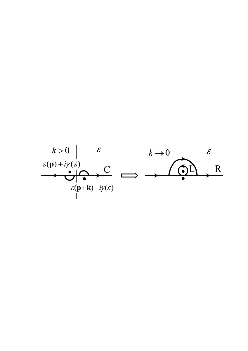
Figure 1: Arrangement of the contour $C$ for the energy integration in Eq. (4)

The term $\rho_{L}$ containing a loop integral absorbs quasiparticle contributions from the poles of $G^{q}$ having the form (2). Implicitly, quasiparticle contributions are also present in a term $\rho_{R}$ associated with integration along the remaining part $R$ of the contour $C$ (see Fig. 1). To prove this we employ the relation AGD

$$-\nabla G^{-1}({\bf p},\varepsilon)={\bf v}_{0}({\bf p})+\int\!\!\!\!\int_{C}\!\!{\cal U}({\bf p},\varepsilon,{\bf l},\omega)\nabla G({\bf l},\omega)\frac{d^{3}{\bf l}\,d\omega}{(2\pi)^{4}i}$$ (6)

derived within many-body theory assuming gauge invariance. Here ${\bf v}_{0}=\nabla\epsilon^{0}_{{\bf p}}$ is the bare group velocity, while ${\cal U}$ represents the block of Feynman diagrams for the scattering amplitude irreducible in the particle-hole channel, and $\nabla=\partial/\partial{\bf p}$.

The first step of our program, adapted from FL theory, is implemented by introducing an interaction amplitude $\Gamma^{R}$ determined by the Landau equation lan2 ; AGD

$$\Gamma^{R}({\bf p},\varepsilon,{\bf p}_{1},\varepsilon_{1})={\cal U}({\bf p},\varepsilon,{\bf p}_{1},\varepsilon_{1})$$

$$+2\int\!\!\!\!\int_{R}\!\!{\cal U}({\bf p},\varepsilon,{\bf l},\omega)G({\bf l},\omega)G({\bf l},\omega)\Gamma^{R}({\bf l},\omega,{\bf p}_{1},\varepsilon_{1})\frac{d^{3}{\bf l}\,d\omega}{(2\pi)^{4}i}.$$ (7)

Hereafter we employ FL symbolic notations, with round brackets implying summation and integration over all intermediate variables, supplemented by respective normalization factors. Thereby Eq. (7) becomes

$$\Gamma^{R}={\cal U}+\Bigl{(}\Gamma^{R}K{\cal U}\Bigr{)}_{\!R}\equiv{\cal U}+\Bigl{(}{\cal U}K\Gamma^{R}\Bigr{)}_{\!R}.$$ (8)

Further, as usual, we multiply Eq. (6) from the left by $\Gamma^{R}GG$ and perform R-integration to obtain

$$-\nabla G^{-1}={\bf v}_{0}+\Bigl{(}\Gamma^{R}K{\bf v}_{0}\Bigr{)}_{\!R}+\Bigl{(}\Gamma^{R}\nabla G\Bigr{)}_{\!L}.$$ (9)

Both Eqs. (8) and (6) were employed to obtain this result. Upon its substitution into the second integral of Eq. (5), one finds

$$\rho_{R}=\Bigl{(}{\bf p}K\nabla G^{-1}\Bigr{)}_{\!R}=-\biggl{(}\Bigl{[}{\bf p}+\Bigl{(}{\bf p}K\Gamma^{R}\Bigr{)}_{\!R}\Bigr{]}K{\bf v}_{0}\biggr{)}_{\!R}$$

$$+\biggl{(}\!\Bigl{(}{\bf p}K\Gamma^{R}\Bigr{)}_{\!R}K\nabla G^{-1}\biggl{)}_{\!\!L}.$$ (10)

After employing the relation migdal ; pit

$$\frac{\partial G^{-1}({\bf p},\varepsilon)}{\partial\varepsilon}{\bf p}={\bf p}+\Bigl{(}{\bf p}K\Gamma^{R}\Bigr{)}_{\!R},$$ (11)

applicable provided the momentum operator ${\bf p}$ commutes with the total Hamiltonian of the system, Eq. (10) is significantly facilitated, taking the form

$$\rho_{R}=\Bigl{(}{\bf p}\Bigl{[}\frac{\partial G^{-1}({\bf p},\varepsilon)}{\partial\varepsilon}-1\Bigr{]}K\nabla G^{-1}\Bigr{)}_{\!\!L},$$ (12)

upon noting that the first term on the r.h.s. of Eq. (10), rewritten as $-\Bigl{(}p_{n}(\partial G^{-1}/\partial\varepsilon)GGv^{0}_{n}\Bigr{)}_{\!R}=\Bigl{(}p_{n}v^{0}_{n}\partial G/\partial\varepsilon\Bigr{)}_{\!R}$, vanishes upon energy integration.

Summation of $\rho_{R}$ from Eq. (12) and $\rho_{L}$ as given by the first of the integrals (5) yields the desired result

$$\rho=\frac{2}{3}\int\!\!\!\!\int_{L}\!\!\frac{\partial G^{-1}({\bf p},\varepsilon)}{\partial\varepsilon}p_{n}K({\bf p},\varepsilon)\frac{\partial G^{-1}({\bf p},\varepsilon)}{\partial p_{n}}\frac{d^{3}{\bf p}\,d\varepsilon}{(2\pi)^{4}i}.$$ (13)

Near the pole, one has $\partial G^{-1}({\bf p},\varepsilon)/\partial\varepsilon=z^{-1}$, while $\nabla G^{-1}({\bf p},\varepsilon)=-z^{-1}\nabla\epsilon({\bf p})$. Given that the Fermi surface (FS) remains simply connected, insertion of these results into Eq. (13) produces

$$\rho=-\frac{2}{3}\int\!\!\!\!\int_{L}p_{n}\frac{\partial G^{q}({\bf p},\varepsilon)}{\partial p_{n}}\frac{d^{3}{\bf p}\,d\varepsilon}{(2\pi)^{4}i}=2\!\int n_{L}({\bf p})\frac{d^{3}p}{(2\pi)^{3}}=\frac{p^{3}_{F}}{3\pi^{2}}.$$ (14)

This result, known as the Landau-Lüttinger (LL) theorem, remains valid as long as the equation

$$\epsilon({\bf p},n_{L})=0$$ (15)

has a single root lifshitz ; volovik . This is indeed the case, provided the change $\delta E(n_{L})=\sum_{{\bf p}}\epsilon({\bf p};n_{L})\delta n_{L}({\bf p})$ of the energy of the Landau state remains non-negative under any variation of the momentum distribution $n_{L}({\bf p})$ compatible with the Pauli principle physrep . This is true for homogeneous Fermi liquids where $\epsilon(p,n_{L})=v_{F}(\rho)(p-p_{F})$, provided the Fermi velocity $v_{F}=p_{F}/m^{*}$ remains positive lan1 . It then follows that the quantities $\epsilon({\bf p})$ and $\delta n({\bf p})$ always have the same sign, to guarantee $\delta E>0$.

Analogous manipulations performed for Eq. (6) lead to the Pitaevskii equation pit

$$\frac{\partial\epsilon({\bf p};n_{L})}{\partial{\bf p}}=\frac{\partial\epsilon_{0}({\bf p})}{\partial{\bf p}}+2\int f({\bf p},{\bf l})\frac{\partial n_{L}({\bf l})}{\partial{\bf l}}\frac{d^{3}{\bf l}}{(2\pi)^{3}}$$ (16)

involving the interaction function $f=z^{2}\Gamma^{R}$. Given its form, Eq. (16) can be solved numerically to yield the quasiparticle spectrum $\epsilon({\bf p};n_{L})$ in all of momentum space physrep ; zkp . However, Eqs. (14) and (16) need to be rearranged when Eq. (15) acquires additional roots that occur if the Fermi velocity $v_{F}$, calculated for the given Landau state, changes sign. In the 2D homogeneous electron liquid of MOSFETs, such a situation occurs at a critical density $\rho_{\infty}=0.8\times 10^{11}\,{\rm cm}^{-2}$ mokashi where both the density of states and the effective mass diverge. Beyond this topological critical point (TCP), countless options for breakdown of the original Landau state arise.

The anisotropy of the electron spectrum in solids furnishes additional opportunities for topological rearrangement of the Landau state. These effects are associated with the inflow of the TCPs where the function $v_{F}(p,{\bf n};n_{L})$ found from Eq. (16) changes sign at certain points of the Fermi surface, occurring automatically if the respective solutions of Eq. (16) attain boundaries of the Brillouin zone. Presumably, such a situation is realized in twisted bilayer graphene (TBLG), where $v_{F}(\rho,\theta)$ passes through zero at a critical twist angle $\theta_{m}\simeq 1.1^{\circ}$, inducing an inevitable topological rearrangement of nearly-flat-band solutions, which have been identified in Ref. bm . In this case, variations $\delta E(n_{L})$ inescapably acquire a negative sign ubiquitously in the whole momentum region where $v_{F}(n_{L})<0$, implying that the number of roots of Eq. (15) becomes infinite again.

A relevant solution of the problem can be found, requiring the associated energy variations

$$\delta E(n_{*})=\sum_{\bf p}\epsilon({\bf p};n_{*})\delta n_{*}({\bf p})$$ (17)

of the state with the rearranged quasiparticle momentum distribution $n_{*}(p)$ to be non-negative. Allowing the permissible occupation numbers $n({\bf p};n_{*})$ to lie between 0 and 1, both signs of $\delta n_{*}({\bf p})$ come into play. Non-negativity of $\delta E(n_{*})$ can then be ensured, provided the energy $\epsilon({\bf p},n_{*})$ vanishes identically in the momentum region $\Omega$. Accordingly, in this regime the single-particle spectrum becomes completely flat ks ; vol1 ; noz ; ktsn1 ; volovik ; prb2008 ; m100 ; annals ; ktsn2 ; book yielding

$$0=\frac{\partial\epsilon_{0}({\bf p})}{\partial{\bf p}}+2\int f({\bf p},{\bf l})\frac{\partial n_{*}({\bf l})}{\partial{\bf l}}\frac{d^{3}{\bf l}}{(2\pi)^{3}},\quad{\bf p}\in\Omega,$$ (18)

while remaining unchanged outside $\Omega$ (except for the obvious replacement $n_{L}\to n_{*}$).

Previously prb2008 ; m100 , we have investigated the fate of the LL theorem in Fermi systems harboring the fermion condensate (FC), where the pole term $G^{q}$ becomes

$$G^{q}({\bf p},\varepsilon)=\frac{1-n_{*}({\bf p})}{\varepsilon-\epsilon({\bf p})+i\gamma(\varepsilon)}+\frac{n_{*}({\bf p})}{\varepsilon-\epsilon({\bf p})-i\gamma(\varepsilon)},$$ (19)

with $\epsilon({\bf p})$ now determined from Eq. (18). In Refs. prb2008 ; m100 , we have obtained the relation

$$\rho=2\int n_{*}({\bf p})\frac{d^{3}{\bf p}}{(2\pi)^{3}},$$ (20)

which also follows from Eq. (14) upon inserting Eq. (19).

A salient feature inherent in states having an interaction-induced flat band is exhibited in the advent of an entropy excess $S_{*}$ given by Landau-like formula

$$\frac{S_{*}}{V}=-2\int_{\Omega}[n_{*}({\bf p})\ln n_{*}({\bf p})+(1-n_{*}({\bf p}))\ln(1-n_{*}({\bf p})]\frac{d^{3}{\bf p}}{(2\pi)^{3}}.$$ (21)

In essence, Eqs. (18)-(21) form the basis of the interaction-induced flat-band scenario, also called the theory of fermion condensation.

Adaptation of the foregoing strategy to the description of superconducting alloys naturally requires the introduction of Gor’kov equations involving two different single-particle Green’s functions AGD ; gor'kov ; migdal ; gor ,

$$G_{s}({\bf p},\varepsilon) = \Bigl{[}G^{-1}({\bf p},\varepsilon)+\Delta^{2}({\bf p})G(-{\bf p},-\varepsilon)\Bigr{]}^{-1},$$

$$F({\bf p},\varepsilon) = G(-{\bf p},-\varepsilon)\Delta({\bf p})G_{s}({\bf p},\varepsilon).$$ (22)

Here the normal-state Green’s function $G({\bf p},\varepsilon)$ obeys formulas (1) and (2), as before.

Within the framework of the BCS approach, the superconducting gap $\Delta$ is supposed to be $p-$ and $\varepsilon-$independent, which greatly facilitates further analysis. Eq. (4) is then replaced by

$$\rho=-\frac{2}{3}\int\!\!\!\!\int_{C}p_{n}\frac{\partial G_{s}({\bf p},\varepsilon)}{\partial p_{n}}\frac{d^{3}{\bf p}\,d\varepsilon}{(2\pi)^{4}i}$$

$$=\frac{2}{3}\int\!\!\!\!\int_{C}\!\!{\bf p}K_{s}({\bf p},\varepsilon)\nabla G^{-1}({\bf p},\varepsilon)\frac{d^{3}{\bf p}\,d\varepsilon}{(2\pi)^{4}i},$$ (23)

where

$$K_{s}({\bf p},\varepsilon)=\lim_{{\bf k}\to 0}[G_{s}({\bf p},\varepsilon)G_{s}({\bf p}+{\bf k},\varepsilon)-F({\bf p},\varepsilon)F({\bf p}+{\bf k},\varepsilon)].$$ (24)

In symbolic notations, one now has

$$\rho_{R} = \Bigl{(}{\bf p}K_{s}\nabla G^{-1}\Bigr{)}_{\!R},\quad\Gamma^{R}={\cal U}+\Bigl{(}\Gamma^{R}K_{s}{\cal U}\Bigr{)}_{\!R},$$

$$-\nabla G^{-1} = {\bf v}_{0}+\Bigl{(}\Gamma^{R}K_{s}{\bf v}_{0}\Bigr{)}_{\!R}+\Bigl{(}\Gamma^{R}\nabla G\Bigr{)}_{\!L},$$

$$\frac{\partial G^{-1}({\bf p},\varepsilon)}{\partial\varepsilon}{\bf p} = {\bf p}+\Bigl{(}{\bf p}K_{s}\Gamma^{R}\Bigr{)}_{\!R}.$$ (25)

These formulas are obtained from those derived for a normal Fermi liquid through the replacement $K\to K_{s}$.

Proceeding farther along the same lines as before, we find

$$\rho_{R}=-\Bigl{(}\frac{\partial G^{-1}}{\partial\varepsilon}K_{s}{\bf v}_{0}\Bigr{)}_{\!R}+\Bigl{(}{\bf p}\Bigl{[}\frac{\partial G^{-1}({\bf p},\varepsilon)}{\partial\varepsilon}-1\Bigr{]}K_{s}\nabla G^{-1}\Bigr{)}_{\!\!L}.$$ (26)

The first term in the sum vanishes again, since $K_{s}\partial G^{-1}/\partial\varepsilon\equiv\partial G_{s}/\partial\varepsilon$, and hence its integration over energy vanishes. Thus we arrive at a nontrivial result: regular (R) contributions to the density $\rho$ associated with the contour R that may in principle depend on the gap value drop out identically, so we are left with the pole contributions (L) tied to the loop contour L. Indeed, upon summation of $\rho_{R}$ with $\rho_{L}$, we are led to

$$\rho=\frac{2}{3}\int\!\!\!\!\int_{L}\!\!\frac{\partial G^{-1}({\bf p},\varepsilon)}{\partial\varepsilon}p_{n}K_{s}({\bf p},\varepsilon)\frac{\partial G^{-1}({\bf p},\varepsilon)}{\partial p_{n}}\frac{d^{3}{\bf p}\,d\varepsilon}{(2\pi)^{4}i}.$$ (27)

Near the quasiparticle pole $G_{s}({\bf p},\varepsilon)=zG^{q}_{s}({\bf p},\varepsilon)$ and $K_{s}({\bf p},\varepsilon)=z^{2}[G_{s}^{q}({\bf p},\varepsilon)G_{s}^{q}({\bf p},\varepsilon)-F^{q}({\bf p},\varepsilon)F^{q}({\bf p},\varepsilon)]$, with LM ; migdal

$$G_{s}^{q}({\bf p},\varepsilon)=\frac{u^{2}({\bf p})}{\varepsilon-E({\bf p})+i\delta}+\frac{v^{2}({\bf p})}{\epsilon+E({\bf p})-i\delta},$$ (28)

and $v^{2}({\bf p})=(E({\bf p})-\epsilon({\bf p}))/2E({\bf p})$, where $E({\bf p})=\sqrt{\epsilon^{2}({\bf p})+\Delta^{2}({\bf p})}$ is the Bogolyubov quasiparticle energy. Upon performing loop integrations in Eq. (27), all the $z$-factors cancel out again to arrive at

$$\rho=-\frac{2}{3}\int\!\!\!\!\int p_{n}\frac{\partial G_{s}^{q}({\bf p},\varepsilon)}{\partial p_{n}}\frac{d^{3}{\bf p}\,d\varepsilon}{(2\pi)^{4}i}=2\!\int\!v^{2}({\bf p})\frac{d^{3}{\bf p}}{(2\pi)^{3}}.$$ (29)

Therewith we have demonstrated the coincidence between the particle and quasiparticle densities in Cooper superconductors, irrespective of the ratio $\Delta/T_{F}$ and the magnitude of the damping $\gamma$ in normal states.

We are now in a position to analyze one of the most challenging results of recent extensive experimental studies of overdoped LSCO compounds. This is the deep connection between anomalous properties of their superconducting and normal states, revealed by comparison of the critical temperature $T_{c}(x)$ of termination of exotic superconductivity with the linear-in-$T$ term $A_{1}(x)$ in the low-$T$ normal-state resistivity $\rho(T>T_{c})=\rho_{0}+A_{1}T+A_{2}T^{2}$ (identified over a decade ago in Refs. hussey1 ; paglione ). This connection is exhibited in a striking correlation between variations of the $T=0$ LSCO superfluid density $\rho_{s0}(x)$ with doping $x$ zaanen and the normal-state coefficient $A_{1}(x)$ bozovic . Permanence of the ratio ${\cal R}(x)=A_{1}(x)/\rho_{s0}(x)$ as a function of doping $x$, as confirmed by data shown in Fig. 2, rules out all attempts to explain the outstanding experimental results of Refs. bozovic ; bozltp ; bozprl within the BCS-AG concept and its modifications. This includes the scaling theory of Refs. broun1 ; broun2 , where the $e-e$ interactions are completely ignored. There the theoretical value of the ratio ${\cal R}(x)$ is identically zero, since the NFL effects are not accounted for in the BCS-AG approach, and therefore $A_{1}$ is simply nonexistent.

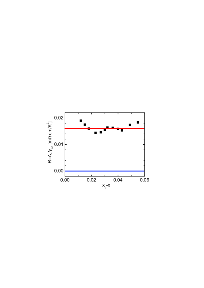
Figure 2: Ratio ${\cal R}(x)=A_{1}(x)/\rho_{s0}(x)$ of the coefficient $A_{1}$ of the linear-in-$T$ term in the low-$T$ normal-state resistivity of La_2-xSr_xCuO₄ compounds to their $T=0$ superfluid density $\rho_{s0}$, versus doping $x$ measured from its critical value $x_{c}$ for gap termination. Black squares show ${\cal R}(x)$ extracted from the data of Ref. bozovic . The horizontal red line illustrates the prediction for ${\cal R}(x)={\rm const.}$ within the FC scenario, its value being chosen to match the experimental data, while the blue line shows the zero value of this ratio within the BCS-AG concept.

On the other hand, the experimental behavior of $A_{1}(x)\propto x_{c}-x$ hussey1 ; paglione ; bozovic is properly explained within the FC scenario, where its value

$$A_{1}(x)\propto\rho_{FC}(x)$$ (30)

turns out to be proportional to the density $\rho_{FC}$ of the fermion condensate. (For details, we refer the reader to recent articles jetplett2015 ; PLA2018 ; RC2020 ).

Evaluation of the superfluid density $\rho_{s}$ reduces to finding the response function $Q_{ij}$ that connects a $T=0$ electric current ${\bf j}$ with the transverse vector potential ${\bf A}$ AGD ,

$$j_{i}({\bf k})=-\frac{\rho e^{2}}{m_{e}}Q_{ij}({\bf k})A_{j}({\bf k}).$$ (31)

One has $Q_{ij}(k)=(\delta_{ij}-k_{i}k_{j}/k^{2})Q(k)$ and $\rho_{s0}=Q(0)\rho$. The function $Q(0)$ is known to contain a vacuum contribution $Q_{\rm vac}=1$ coming from the term $\delta^{2}{\cal H}=e^{2}A^{2}/2m_{e}$ in the corresponding second variation of the vacuum Hamiltonian ${\cal H}$, which responsible, notably, for light scattering by electrons. Thereby one obtains $Q(0)=1+P_{s}(0)$. Importantly, in evaluation of the current-current correlator $P_{s}(0)$, the propagator $L_{s}=G_{s}G_{s}+FF$ replaces $K_{s}=G_{s}G_{s}-FF$ AGD (which enters in the above proof of the LL-like theorem in superconducting systems). Otherwise, the renormalization is carried out along the same lines as in the foregoing proof of the equality between the quasiparticle and particle numbers to yield prb2019

$$\rho_{s0}(x)/\rho=I(x)/[1+(\alpha-1)(1-I(x))],$$ (32)

where $\alpha=m^{*}/m_{e}$ and

$$I(x)\propto\int\!\!\!\int F^{2}(\epsilon,\zeta)\,d\epsilon\,d\zeta=\int\!\!\!\int\frac{\Delta^{2}\eta^{2}(\zeta)\,d\epsilon\,d\zeta}{\Bigl{(}(\zeta^{2}+\Delta^{2})\eta^{2}(\zeta)+\epsilon^{2}\Bigr{)}^{2}},$$ (33)

with

$$\eta(\zeta)=\frac{1}{2}\left(1+\frac{\gamma}{2\sqrt{\zeta^{2}+\Delta^{2}}}\right)\qquad\qquad\qquad\qquad$$

$$+\left[\frac{1}{4}\left(1+\frac{\gamma}{2\sqrt{\zeta^{2}+\Delta^{2}}}\right)^{2}+\frac{\gamma}{\pi}\frac{\rho_{FC}}{\rho}\frac{\varepsilon_{F}}{\zeta^{2}+\Delta^{2}}\right]^{1/2}.$$ (34)

The FC contribution to the integral (34) is found to be insignificant at small FC density $\rho_{FC}$ because this contribution is proportional to $\Delta_{0}\rho_{FC}$. Thus, the result of our calculations prb2019 , namely

$$\rho_{s0}(x)\propto\Delta_{0}(x)\frac{m_{e}}{\gamma_{tr}m^{*}},$$ (35)

turns out to be correct at any $x_{c}-x$. Since the gap value $\Delta_{0}$ is proportional to the FC density $\rho_{FC}$ as well ks ; jetpl2017 , the function ${\cal R}(x)$ is indeed doping-independent, in agreement with experiment.

This article is a logical complement to earlier work addressing the origin of topological disorder RC2020 arising in strongly correlated electron systems. The quasiparticle formalism developed here furnishes the proper theoretical foundation for the analysis of such phenomena. Importantly, this formalism applies to superconducting states with nontrivial topology as well, providing the basis for quantitative analysis of interaction-induced effects in cuprates and other high-$T_{c}$ superconductors, including magic-angle TBLG where the standard near-flat-band solutions bm must experience a topological rearrangement.

In conclusion, the authors are deeply grateful to V. Shaginyan and G. Volovik for discussing issues addressed in this article.

References

(1) J. Bardeen, L. N. Cooper, J. R. Schrieffer, Phys. Rev. 106, 162 (1957); 108, 1175 (1957).
(2) L. P. Gor’kov, Sov. Phys. JETP 7, 505 (1958).
(3) G. M. Eliashberg, Sov. Phys. JETP 11, 696 (1960).
(4) L. N. Cooper, Phys. Rev. 104, 1159 (1957).
(5) L. D. Landau, Sov. Phys. JETP 3, 920 (1957).
(6) L. D. Landau, Sov. Phys. JETP 8, 70 (1958).
(7) A. I. Larkin, A. B. Migdal, Sov. Phys. JETP 17,1146 (1963).
(8) A. B. Migdal, Theory of Finite Fermi Systems and Applications to Atomic Nuclei (Wiley, New York, 1967).
(9) A. A. Abrikosov, L. P. Gor’kov, Sov. Phys. JETP, 8, 1090, (1959); ibid12, 1243 (1960).
(10) V. A. Khodel, J. W. Clark, M. V. Zverev, Phys. Rev. B99, 184503 (2019).
(11) J. G. Bednorz, K. A. Müller, Z. Phys. B64, 189 (1986).
(12) A. J. Leggett, Lecture Notes on Exotic Superconductivity, University of Tokyo Open Course Ware, June 2011.
(13) J. Zaanen, Nature 536, 282 (2016).
(14) I. Bozovic̀, X. He, J. Wu, A. T. Bollinger, Nature 536, 309 (2016).
(15) F. Mahmood, X. He, I. Bozovic̀, N. P. Armitage, Phys. Rev. Lett. 122, 027003 (2019).
(16) I. Bozovic̀, A. T. Bollinger, J. Wu, X. He, Low Temp. Phys. 44, 519 (2018).
(17) A. A. Abrikosov, L. P. Gor’kov, I. E. Dzjaloshinskii, Methods of Quantum Field Theory in Statistical Physics (Pergamon Press, Oxford, 1965).
(18) Y. Cao et al., Phys. Rev. Lett. 124, 076801 (2020).
(19) A. B. Migdal, Sov. Phys. JETP 5, s333 (1957).
(20) L. P. Pitaevskii, Sov. JETP 10, 1267 (1960).
(21) I. M. Lifshitz, Sov. Phys. JETP 11, 1130 (1960).
(22) G. E. Volovik, Springer Lecture Notes in Physics 718, 31 (2007).
(23) V. A. Khodel, V. V. Khodel and V. R. Shaginyan, Phys. Rep. 249, 1 (1994).
(24) M. V. Zverev, V. A. Khodel, S. S. Pankratov, JETP Lett. 96, 192 (2012).
(25) A. Mokashi et al., Phys. Rev. Lett. 109, 096405 (2012).
(26) R. Bistritzer and A. H. McDonald, Proc. Natl. Acad. Sci. U.S.A. 108, 12233 (2011).
(27) G. E. Volovik, JETP Lett. 53, 222 (1991).
(28) V. Yu. Irhin, A. A. Katanin, M. I. Katsnelson, Phys. Rev. Lett. 89, 076401 (2002).
(29) V. A. Khodel and V. R. Shaginyan, JETP Lett. 51, 553 (1990).
(30) P. Nozières, J. Phys. I France 2, 443 (1992).
(31) V. A. Khodel, J. W. Clark, M. V. Zverev, Phys. Rev. B 78, 075120 (2008).
(32) V. A. Khodel, J. W. Clark, M. V. Zverev, Phys. At. Nucl. 74, 1237 (2011).
(33) J. W. Clark, M. V. Zverev, V. A. Khodel, Ann. Phys. 327, 3063 (2012).
(34) D. Yudin et al., Phys. Rev. Lett. 112, 070403 (2014).
(35) M. Ya. Amusya, V. R. Shaginyan, Strongly Correlated Fermi systems: A New State of Matter, Springer Tracts in Modern Physics Vol. 283 (Springer International Publishing, 2020).
(36) L. P. Gor’kov, Theory of Superconducting Alloys, edited by K. H. Bennemann and J. B. Ketterson, Superconductivity Vol. 1 (Springer-Verlag, New York, 2008).
(37) R. A. Cooper et al., Science 323, 603 (2009).
(38) K. Jin et al., Nature 476, 73 (2011).
(39) N. R. Lee-Hone et al., Phys. Rev. 96, 024501 (2017).
(40) N. R. Lee-Hone et al., Phys. Rev. 98, 054506 (2018).
(41)V. A. Khodel et al., JETP Lett. 101, 413 (2015).
(42) V. A. Khodel, J. W. Clark, M. V. Zverev, Phys. Lett. A 382, 3281 (2018).
(43) V. A. Khodel, J. W. Clark, M. V. Zverev, JETP Lett. A 105, 267 (2017).
(44) V. A. Khodel, J. W. Clark, M. V. Zverev, Phys. Rev. B 102, 201108(R) (2020).