Higher Order Generalization Error for
First Order Discretization of Langevin Diffusion

Abstract

We propose a novel approach to analyze generalization error for discretizations of Langevin diffusion, such as the stochastic gradient Langevin dynamics (SGLD). For an $\epsilon$ tolerance of expected generalization error, it is known that a first order discretization can reach this target if we run $\Omega(\epsilon^{-1}\log(\epsilon^{-1}))$ iterations with $\Omega(\epsilon^{-1})$ samples. In this article, we show that with additional smoothness assumptions, even first order methods can achieve arbitrarily runtime complexity. More precisely, for each $N>0$, we provide a sufficient smoothness condition on the loss function such that a first order discretization can reach $\epsilon$ expected generalization error given $\Omega(\epsilon^{-1/N}\log(\epsilon^{-1}))$ iterations with $\Omega(\epsilon^{-1})$ samples.

1 Introduction

Let $f:\mathbb{R}^{d}\times\mathcal{Z}\to\mathbb{R}$ be a known loss function with respect to parameters $x\in\mathbb{R}^{d}$ and a single data point $z\in\mathcal{Z}$. We define $F(x):=\mathbb{E}\,f(x,z)$ where the expectation is over $z\sim\mathcal{D}$ for an unknown distribution $\mathcal{D}$ over $\mathcal{Z}$. We consider the problem of minimizing an expected loss function

$$\min_{x\in\mathbb{R}^{d}}F(x)\,.$$ (1.1)

Since the distribution is unknown, we rely on a sample of $n$-independent and identically distributed (i.i.d.) data points $\mathbf{z}=\{z_{i}\}_{i=1}^{n}\sim\mathcal{D}^{n}$, and evaluate the empirical loss function denoted by $F_{\mathbf{z}}(x):=\frac{1}{n}\sum_{i=1}^{n}f(x,z_{i})$. In this setting, a learning algorithm is a random map $X:\mathcal{Z}^{n}\to\mathbb{R}^{d}$, and we use $X_{\mathbf{z}}$ to denote the output. Since the empirical loss $F_{\mathbf{z}}(X_{\mathbf{z}})$ can be evaluated, it remains to study the expected generalization error

$$\mathbb{E}\,F(X_{\mathbf{z}})-\mathbb{E}\,F_{\mathbf{z}}(X_{\mathbf{z}})\,,$$ (1.2)

where the expectation is over both the randomness of $X$ and $\mathbf{z}\sim\mathcal{D}^{n}$.

In this article, we are interested in the class of algorithms that can be viewed as a discretization of the (overdamped) Langevin diffusion, defined by the stochastic differential equation (SDE)

$$dX(t)=-\nabla F_{\mathbf{z}}(X(t))\,dt+\sqrt{\frac{2}{\beta}}\,dW(t)\,,$$ (1.3)

where $\beta>0$ is the inverse temperature parameter, and $\{W(t)\}_{t\geq 0}$ is a standard Brownian motion in $\mathbb{R}^{d}$. It is well known that the Langevin diffusion converges (as $t\to\infty$) to the Gibbs distribution $\rho_{\mathbf{z}}(x)\propto\exp(-\beta F_{\mathbf{z}}(x))$ (Bakry et al., 2013). Furthermore, using the uniform stability condition introduced by Bousquet and Elisseeff (2002), the Gibbs distribution is shown to have generalization error $O(n^{-1})$ (Raginsky et al., 2017). Many optimization results also rely on the Gibbs distribution’s minimizing property (Raginsky et al., 2017; Xu et al., 2017; Erdogdu et al., 2018).

Using this approach, Xu et al. (2017) studied a first order discretization of the Langevin diffusion $\{X_{\mathbf{z},k}\}_{k\geq 0}$ with step size $\eta>0$, and showed the approximation error between the algorithm and the Gibbs distribution is on the order of $O(e^{-\Omega(k\eta)}+\eta)$, where $k>0$ is the number of iterations. In terms of runtime and sample complexity for an $\epsilon$ tolerance on generalization error, this implies we need to choose a small step size $\eta=O(\epsilon)$, leading to $k\geq\Omega(\epsilon^{-1}\log\epsilon^{-1})$ and $n\geq\Omega(\epsilon^{-1})$. This approach corresponds to the top path of approximation steps to generalization error in Figure 1.

Figure 1: Overview of approximation steps taken to bound the generalization error $\mathbb{E}\,F_{\mathbf{z}}(X_{\mathbf{z},\infty})-\mathbb{E}\,F(X_{\mathbf{z},\infty})$. Here we use $X_{\mathbf{z},\infty}$ to denote a sample from the stationary distribution, $O(\cdot)$ to display an approximation error bound with dependence on step size $\eta$ and number of samples $n$, and $\rho_{\mathbf{z}}(F)$ to denote the integral $\int F\,d\rho_{\mathbf{z}}$.

In contrast to previous works, our approach avoids viewing first order methods as a discretization of Langevin diffusion. Instead, we view first order methods as higher order discretizations of a modified process, which we construct via weak backward error analysis (Debussche and Faou, 2011; Kopec, 2013, 2015). With the explicit construction, we can recover the stationary distribution $\pi^{N}_{\mathbf{z}}$ of the modified process, which approximates the first order methods to order $O(\eta^{N})$, where $N>0$ depends on the smoothness of $f(\cdot,z)$. Then our main result establishes a generalization bound of $O(n^{-1})$ for this distribution $\pi^{N}_{\mathbf{z}}$, which is of the same order as Gibbs. As a result, our approach shows that the generalization property of Gibbs is actually a generic property of Poisson equations. Putting these together, our results imply we can choose a much larger stepsize of $\eta=O(\epsilon^{1/N})$, leading to an improved runtime complexity of $k\geq\Omega(\epsilon^{-1/N}\log\epsilon^{-1})$ while keeping the same sample complexity of $n\geq\Omega(\epsilon^{-1})$. This is described in the bottom path in Figure 1.

We summarize our main contributions as follows. We provide an explicit construction of the modified process approximating SGLD, as well as the stationary distribution $\pi^{N}_{\mathbf{z}}$, up to an error of order $O(\eta^{N})$. Under additional smoothness conditions, we provide an improved generalization bound for first order discretizations of Langevin diffusion.

The rest of the article is organized as follows. We discuss related works and comparison next in Section 1.1. In Section 2, we introduce the precise notation and main results. In Section 3, we provide an overview of the proofs, deferring technical details to the appendix. In Section 4, we discuss the assumptions and further extensions of this work. In Sections 5, 6 and 7, we provide the proof of the main results in full detail.

1.1 Related Works

Langevin algorithms for sampling and optimization have been very well studied (Gelfand and Mitter, 1991; Raginsky et al., 2017; Cheng et al., 2018; Dalalyan and Karagulyan, 2019; Durmus and Moulines, 2017; Erdogdu et al., 2018; Li et al., 2019; Vempala and Wibisono, 2019; Erdogdu and Hosseinzadeh, 2020). Most of these articles establish approximations using the Langevin diffusion, either in finite time or in terms of stationary distributions. In particular, several existing works have studied the approximation of stationary distributions (Talay and Tubaro, 1990; Mattingly et al., 2010; Erdogdu et al., 2018). This line of work is most similar to our approach in studying the error in the distributional sense.

Paper	Regularity Assumptions	Steps $k\geq\Omega(\cdot)$ to reach $\epsilon$ generalization error
Raginsky et al. (2017)	Gradient Lipschitz	$\epsilon^{-4}(\log(\epsilon^{-1}))^{3}$
Xu et al. (2017)	Gradient Lipschitz	$\epsilon^{-1}\log(\epsilon^{-1})$
Erdogdu et al. (2018)	$f(\cdot,z)\in C^{4}_{\operatorname{pol}}$	$\epsilon^{-2}$
Present Work	Gradient Lipschitz, $f(\cdot,z)\in C^{6N+2}_{\operatorname{pol}}$	$\epsilon^{-1/N}\log(\epsilon^{-1})$

Table 1: Comparison of the assumptions and resulting runtime complexities to reach $\epsilon$ approximation error by recent works. Here $C^{\ell}_{\operatorname{pol}}$ denotes the space of $C^{\ell}$ functions where all derivatives have polynomial growth, and $\Omega(\,\cdot\,)$ notation hides constants independent of $\epsilon$. We emphasize that all previous works have approximated the Langevin algorithm using the Gibbs density, while the present work constructs a modified density. We provide precise details on assumptions and results in Section 2.

The idea of backward error analysis traces back to the study of numerical linear algebra (Wilkinson, 1960) and numerical methods for ordinary differential equations (ODEs) (Hairer et al., 2006). This approach views each update step of a numerical algorithm as the exact solution of a modified differential equation. For example, if we solve the ODE $y^{\prime}(t)=y(t)^{2}$ with the Euler update $y_{k+1}=y_{k}+\eta y_{k}^{2}$ for some $\eta>0$, then the modified equation can be written as an infinite series (Hairer et al., 2006, Chapter IX, Example 1.1)

$$\widetilde{y}^{\prime}=\widetilde{y}^{2}-\eta\widetilde{y}^{3}+\eta^{2}\frac{3}{2}\widetilde{y}^{4}-\eta^{3}\frac{8}{3}\widetilde{y}^{5}+\eta^{4}\frac{31}{6}\widetilde{y}^{6}+\cdots\,,$$

where given initial condition $\widetilde{y}(0)=y_{k}$, we will have that $\widetilde{y}(\eta)=y_{k+1}$.

However, directly extending this construction to SDEs pathwise is not straightforward (Shardlow, 2006). Instead, Debussche and Faou (2011) introduced a construction approximating the numerical method in distribution. The authors derived a partial differential equation (PDE) describing the evolution of the distribution for the numerical algorithm, and consequently the stationary distribution as well. We will provide more details in Section 3. This work has been extended to implicit Langevin algorithms (Kopec, 2013, 2015), higher order discretizations (Abdulle et al., 2012, 2014; Laurent and Vilmart, 2020), and stochastic Hamiltonian systems with symplectic schemes (Wang et al., 2016; Anton, 2017, 2019).

We summarize a comparison of related approximation results for SGLD in Table 1.

2 Main Results

Throughout the article we denote the Euclidean inner product by $\langle x,y\rangle$ for $x,y\in\mathbb{R}^{d}$, and the corresponding norm by $\left|x\right|:=\langle x,x\rangle^{1/2}$. Unless otherwise specified, all expectations $\mathbb{E}[\,\cdot\,]$ are with respect to all sources of randomness including ${\mathbf{z}}$. We denote the conditional expectation on a random variable using the subscript notation, more precisely we use $\mathbb{E}_{\mathbf{z}}[\,\cdot\,]:=\mathbb{E}[\,\cdot\,|{\mathbf{z}}]$. For any measure or density $\pi$ on $\mathbb{R}^{d}$, we denote the integral $\int\phi\,d\pi$ as $\pi(\phi)$. We also use the subscript notation on distributions $\pi_{\mathbf{z}}$ (and other objects) to denote the dependence on the dataset $\mathbf{z}\in\mathcal{Z}^{n}$.

Given a multi-index $\alpha=(\alpha_{1},\ldots,\alpha_{d})\in\mathbb{N}^{d}$, we define $|\alpha|=\alpha_{1}+\cdots+\alpha_{d}$. For any function $\phi\in C^{\infty}(\mathbb{R}^{d})$, we define the short hand derivative notation $\partial_{\alpha}\phi(x)=(\partial_{x_{1}})^{\alpha_{1}}\cdots(\partial_{x_{d}})^{\alpha_{d}}\phi(x)$. For all $k,\ell\in\mathbb{N}$, we also define the function norm $\|\phi\|_{k,\ell}:=\sup_{\begin{subarray}{c}|\alpha|\leq k\end{subarray}}\,\sup_{x\in\mathbb{R}^{d}}|\partial_{\alpha}\phi(x)|(1+|x|^{\ell})^{-1}.$ This leads to the natural function space $C^{k}_{\ell}(\mathbb{R}^{d}):=\{\phi\in C^{k}(\mathbb{R}^{d}):\|\phi\|_{k,\ell}<\infty\}$.

We are now ready to state the main assumptions on the loss function $f(x,z)$.

Assumption 2.1 (Regularity).

There exists positive integers $N,\ell$ such that $f(\cdot,z)\in C^{6N+2}_{\ell}(\mathbb{R}^{d})$ and $\sup_{z\in\mathcal{Z}}\|f(\cdot,z)\|_{6N+2,\ell}<\infty$. Furthermore, there exists a constant $M>0$ such that

$$\left|\nabla f(x,z)-\nabla f(y,z)\right|\leq M\left|x-y\right|,\quad\forall x,y\in\mathbb{R}^{d}\,.$$ (2.1)

Without loss of generality, this assumption implies for each $\alpha\in\mathbb{N}^{d}$ with $|\alpha|\leq 6N+2$, there exists a constant $M_{\alpha}>0$ such that $\sup_{z\in\mathcal{Z}}|\partial_{\alpha}f(x,z)|\leq M_{\alpha}(1+|x|^{\ell})$. For each $k\in\mathbb{N}$, we define $M_{k}=\sum_{|\alpha|=k}M_{\alpha}$.

Assumption 2.2 (Dissipative).

There exist constants $m>0$ and $b\geq 0$ such that

$$\langle x,\nabla f(x,z)\rangle\geq m\left|x\right|^{2}-b,\quad\forall x\in\mathbb{R}^{d},z\in\mathcal{Z}.$$ (2.2)

We remark this is a commonly used sufficient condition for exponential convergence of Langevin diffusion (Raginsky et al., 2017; Bakry et al., 2008), and it can be replaced by any other sufficient condition (Villani, 2009; Bakry et al., 2013).

We define stochastic gradient Langevin dynamics (SGLD) by the following update rule

$$X_{k+1}=X_{k}-\eta\nabla F_{\zeta_{k}}(X_{k})+\sqrt{\frac{2\eta}{\beta}}\xi_{k}\,,$$ (2.3)

where $X_{0}=x\in\mathbb{R}^{d}$ is a deterministic initial condition, $\eta>0$ is a constant step size (or learning rate), $\beta>0$ is the inverse temperature parameter, $\{\zeta_{k}\}_{k\in\mathbb{N}}$ are uniform (minibatch) subsamples of ${\mathbf{z}}$ (with replacement) of size $n_{b}\leq n$, and $\{\xi_{k}\}_{k\in\mathbb{N}}$ are i.i.d. samples from $\mathcal{N}(0,I_{d})$. Here we let $\{\zeta_{k}\}_{k\in\mathbb{N}},\{\xi_{k}\}_{k\in\mathbb{N}}$ be independent conditioned on ${\mathbf{z}}$.

We are ready to state our first main result.

Theorem 2.3 (Approximation of SGLD).

Suppose $f(x,z)$ satisfies Assumption 2.1 and 2.2 with order of approximation $N\in\mathbb{N}$. Then there exist positive constants $C,\lambda,\ell^{\prime}$ (depending on $N$), such for all step sizes $0<\eta<\frac{2m}{M^{2}}$ and $\mathbf{z}\in\mathcal{Z}^{n}$, we can construct a modified stationary measure $\pi^{N}_{\mathbf{z}}$, with the property that for all steps $k\geq 0$, initial condition $X_{0}=x$, and test function $\phi\in C^{6N+2}_{\ell}(\mathbb{R}^{d})$, the following approximation bound on the SGLD algorithm $\{X_{k}\}_{k\geq 0}$ (2.3) holds

$$\left|\,\mathbb{E}_{\mathbf{z}}\,\phi(X_{k})-\pi^{N}_{\mathbf{z}}(\phi)\,\right|\leq C\left(e^{-\lambda k\eta/2}+\eta^{N}\right)(1+|x|)^{\ell^{\prime}}\,\|\phi-\rho_{\mathbf{z}}(\phi)\|_{6N+2,\ell}\,.$$ (2.4)

In particular, the above result holds for $\phi\in\{F,F_{\mathbf{z}}\}$.

The full proof can be found in Section 5.

Our second main result is on bounding the generalization error of the approximate stationary distribution. Here we note that beyond SGLD, many discretizations of Langevin diffusion admits a higher order approximate stationary distribution $\pi^{N}_{\mathbf{z}}$ via the same weak backward error analysis construction. In particular, the implicit Euler method (Kopec, 2013) and weak Runge-Kutta methods (Laurent and Vilmart, 2020) are well studied. Therefore, we state the result for all such methods.

Theorem 2.4 (Generalization Bound of $\pi^{N}_{\mathbf{z}}$).

Suppose $\{X_{k}\}_{k\geq 0}$ is any discretization of Langevin diffusion (1.3) with an approximate stationary distribution $\pi^{N}_{\mathbf{z}}$ as in Theorem 2.3. Then there exists a constant $C>0$ (depending on $N$), such that for all choices of $k,n$ and $\eta\in(0,1)$ the following expected generalization bound holds

$$\left|\,\mathbb{E}\left[\pi^{N}_{\mathbf{z}}(F)-\pi^{N}_{\mathbf{z}}(F_{\mathbf{z}})\right]\,\right|\leq\frac{C}{n(1-\eta)}\,,$$ (2.5)

where the expectation is with respect to $\mathbf{z}\sim\mathcal{D}^{n}$.

The full proof can be found in Section 6. As a corollary of the two results, we have a runtime complexity as follows.

Corollary 2.5 (Runtime Complexity).

Suppose $\{X_{k}\}_{k\geq 0}$ is any discretization of Langevin diffusion (1.3) admiting an approximate stationary distribution $\pi^{N}_{\mathbf{z}}$ of the type in Theorem 2.3. Then there exists a constant $C>0$ (depending on $N$), such that for all

$$\epsilon>0\,,\quad 0<\eta<\min\left\{\frac{2m}{M^{2}}\,,C\epsilon^{1/N}\right\}\,,\quad n\geq\frac{C}{\epsilon(1-\eta)}\,,\quad k\geq\frac{C}{\epsilon^{1/N}}\log\frac{1}{\epsilon}\,,$$ (2.6)

we achieve the following expected generalization bound

$$\left|\,\mathbb{E}\left[F(X_{k})-F_{\mathbf{z}}(X_{k})\right]\,\right|\leq\epsilon\,.$$ (2.7)

The proof can be found in Section 7. Once again, we remark this implies a runtime complexity of $k\geq\Omega(\epsilon^{-1/N}\log(\epsilon^{-1}))$ despite $\{X_{k}\}_{k\geq 0}$ being a first order discretization of Langevin diffusion.

3 Proof Overview

In this section, we provide a sketch of the main results. Here we omit most of the technical details, with the goal of explaining the core ideas clearly and concisely.

3.1 Construction of $\pi^{N}_{\mathbf{z}}$

Before we go to the distributional setting, it is instructive to build intuitions from ODEs. In particular, we return to (Hairer et al., 2006, Chapter IX, Example 1.1), where we consider solving $y^{\prime}(t)=y(t)^{2}$ with the Euler update $y_{k+1}=y_{k}+\eta y_{k}^{2}$ for some $\eta>0$. Following this example, we hypothesize the existence of a modified ODE as the formal series

$$\widetilde{y}^{\prime}(t)=\widetilde{y}(t)^{2}+\sum_{\ell=1}^{\infty}c_{\ell}(\widetilde{y}(t))\,\eta^{\ell}\,,$$ (3.1)

such that $\widetilde{y}(0)=y_{k}$ and $\widetilde{y}(\eta)=y_{k+1}$. If $\widetilde{y}$ has a Taylor expansion satisfying the constraint $\widetilde{y}(\eta)=\widetilde{y}(0)+\eta\widetilde{y}(0)^{2}$, we can solve for all the coefficients $c_{\ell}(\widetilde{y}(t))$ by matching the terms with the same polynomial order of $\eta^{\ell}$.

Observe that if this formal series converges, we have an exact reconstruction of the Euler method $\{y_{k}\}_{k\geq 1}$ via a modified ODE. However, since this is often not easy (or even possible), we alternatively consider a truncation of this series, leading to a high order approximation. This is exactly the approach known as backward error analysis (Hairer et al., 2006). We plot this particular example in Figure 2.

(a) (b)

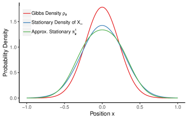
Figure 2: (a): A plot of backward error analysis for the example ODE (3.1), where truncations of $\widetilde{y}(t)$ are taken to better approximate the Euler discretization. (b): A toy example to show how the distribution $\pi^{N}_{\mathbf{z}}$ constructed using weak backward error analysis compares against the true stationary distribution of SGLD $\mathcal{L}(X_{\infty})$. In this case, we choose the loss to be $f(x,z)=\frac{1}{2}x^{2}$ so we can obtain explicit formulas for the densities. We observe a large discrepancy between the Gibbs measure $\rho_{\mathbf{z}}$ and $\mathcal{L}(X_{\infty})$ (for SGLD), where as the first order approximation $\pi^{1}_{\mathbf{z}}$ is a much better approximation to $\mathcal{L}(X_{\infty})$. See Appendix B for details of the calculations.

Once again, we emphasize that extending this method directly through pathwise approximation of the diffusion will be difficult (Shardlow, 2006). However, if we forego the pathwise information of the Langevin diffusion $\{X(t)\}_{t\geq 0}$ (1.3), and only consider its distribution via $\mathbb{E}\phi(X(t))$ for some test function $\phi$, we can study the evolution via the Kolmogorov backward equation

$$\partial_{t}u(t,x)=L_{\mathbf{z}}\,u(t,x)\,,\quad u(0,x)=\phi(x)\,,$$ (3.2)

where $L_{\mathbf{z}}\,u:=\langle-\nabla F_{\mathbf{z}},\nabla u\rangle+\frac{1}{\beta}\Delta u$ is the Itô generator, and $u(t,x)=\mathbb{E}[\phi(X(t))|X_{0}=x]$ is the well known stochastic representation (Pardoux and Răşcanu, 2014, Theorem 3.43).

Since the evolution of Langevin diffusion’s distribution can be interpreted as Wasserstein gradient flow in the space of probability distributions (Jordan et al., 1998), it is natural to consider extending backward error analysis in the space of distributions. Indeed, this is the approach taken by Debussche and Faou (2011) using a modified PDE instead.

Similar to 3.1, we instead write down a modified Kolmogorov equation as a formal series

$$\partial_{t}v=L_{\mathbf{z}}v+\sum_{\ell=1}^{\infty}\eta^{\ell}\,L_{\ell,\mathbf{z}}\,v\,,\quad v(0,x)=\phi(x)\,,$$ (3.3)

where $\{L_{\ell,\mathbf{z}}\}_{\ell\geq 1}$ are differential operators playing the same role as the coefficients $c_{\ell}$ in 3.1. These operators are solved such that an Itô type Taylor expansion matches the distribution of SGLD in the sense $v(\eta,x)=\mathbb{E}[\phi(X_{1})|X_{0}=x]$ formally, where $X_{1}$ is the one step update of 2.3 and $\phi$ is the same test function as in 3.3.

Once again, this formal series is an exact reconstruction of SGLD’s evolution if the series is convergent. Similar to the modified equation for ODEs, we avoid justifying the convergence by taking a truncation at order $N$, matching the regularity condition of Assumption 2.1, which is required for the Taylor type expansion in $\eta$. More precisely, we construct the truncation using functions $v_{m}(t,x)$ defined recursively as the solutions of the following equations

$$\partial_{t}v_{m}-L_{\mathbf{z}}v_{m}=\sum_{\ell=1}^{m}L_{\ell,\mathbf{z}}v_{m-\ell}\,,\quad v_{m}(0,x)=\begin{cases}\phi(x)\,,&m=0\,,\\ 0\,,&m>0\,.\end{cases}$$ (3.4)

Using this construction, we show that the truncation of $v$ defined by $v^{(N)}=\sum_{\ell=0}^{N}\eta^{\ell}v_{\ell}$ approximates $\mathbb{E}[\phi(X_{1})|X_{0}=x]$ up to an error of $O(\eta^{N+1})$ .

Next, we establish the convergence of the truncation terms $v_{m}$ via a standard spectral gap argument for non-homogenous parabolic PDEs (Pardoux et al., 2003). More precisely, we can write

$$\left|v_{m}(t,x)-\lim_{s\to\infty}v_{m}(s,x)\right|\leq C\,e^{-\lambda t/2}\,,$$ (3.5)

where $\lambda>0$ is the Poincaré constant arising as a consequence of Assumption 2.2 (Bakry et al., 2008; Raginsky et al., 2017). By standard adjoint equation arguments (Pavliotis, 2014, Theorem 2.2), we can recover the stationary measure from (3.4) by setting $\partial_{t}v_{m}=0$ and replacing all differential operators with their corresponding adjoint. More precisely, we have $\lim_{t\to\infty}v_{m}(t,x)=\rho_{\mathbf{z}}(\phi\,\mu_{m,\mathbf{z}})$, where the Radon-Nikodym derivative $\mu_{m,\mathbf{z}}(x)$ is the unique solution of the Poisson equation

$$L_{\mathbf{z}}\mu_{m,\mathbf{z}}=-\sum_{\ell=1}^{m}L_{\ell,\mathbf{z}}^{*}\mu_{m-\ell,\mathbf{z}}\,,$$ (3.6)

where we use $L_{\ell,\mathbf{z}}^{*}$ to denote the adjoint operator of $L_{\ell,\mathbf{z}}$ in $L^{2}(\rho_{\mathbf{z}})$, and $\mu_{0,\mathbf{z}}=1$. Observe the above equation is exactly stationary adjoint of (3.4), where we note $L_{\mathbf{z}}^{*}=L_{\mathbf{z}}$ is self-adjoint.

Using linearity of expectation over $\rho_{\mathbf{z}}$, we can write

$$\lim_{t\to\infty}v^{(N)}(t,x)=\rho_{\mathbf{z}}\left(\phi\,\sum_{\ell=0}^{N}\eta^{\ell}\,\mu_{\ell,\mathbf{z}}\right)\,,$$ (3.7)

hence we recover the approximate stationary measure as $\pi^{N}_{\mathbf{z}}=\rho_{\mathbf{z}}\sum_{\ell=0}^{N}\eta^{\ell}\mu_{\ell,\mathbf{z}}$.

Finally, to extend the one step error bound of $O(\eta^{N+1})$ to arbitrary steps, we use a telescoping argument to write

$$\left|\,\mathbb{E}_{\mathbf{z}}\,\phi(X_{k})-v^{(N)}(t,x)\,\right| \leq\mathbb{E}\,\sum_{\ell=1}^{k}\,\left|\mathbb{E}[v^{(N)}((\ell-1)\eta,X_{k-\ell+1})-v^{(N)}(\ell\eta,X_{k-\ell})|\mathcal{F}_{k-\ell}]\right|$$ (3.8)

$$\leq C\,\eta^{N+1}\sum_{\ell=1}^{k}e^{-\lambda\ell\eta/2}\,,$$

where $\{\mathcal{F}_{k}\}_{k\geq 0}$ is the filtration generated by the algorithm $\{X_{k}\}_{k\geq 0}$. Here, we used the one step error bound and exponential convergence (3.5). Note that we can bound the geometric series by $\frac{1}{1-e^{-\lambda\eta/2}}=O(\eta^{-1})$, hence leading to the error order of $O(\eta^{N})$ in Theorem 2.3. We plot an example construction of $\pi^{1}_{\mathbf{z}}$, where we can compute the density explicitly in Figure 2.

3.2 Generalization Bound

We start by recalling the definition and generalization property of the uniform stability (Bousquet and Elisseeff, 2002) for distributions.

Definition 3.1 (Uniform Stability).

A collection of distributions $\{\pi_{\mathbf{z}}\}$ on $\mathbb{R}^{d}$ indexed by $\mathbf{z}\in\mathcal{Z}^{n}$ is said to be $\epsilon$-uniformly stable if for all $\mathbf{z},\overline{\mathbf{z}}\in\mathcal{Z}^{n}$ with only one differing coordinate

$$\sup_{z\in\mathcal{Z}}\left|\pi_{\mathbf{z}}(f(\cdot,z))-\pi_{\overline{\mathbf{z}}}(f(\cdot,z))\right|\leq\epsilon.$$ (3.9)

Proposition 3.2 (Generalization).

Suppose the collection of distributions $\{\pi_{\mathbf{z}}\}$ is $\epsilon$-uniformly stable, and that for all $(\mathbf{z},z)\in\mathcal{Z}^{n+1}$, we also have $f(\cdot,z)\in L^{1}(\pi_{\mathbf{z}})$. Then the expected generalization error of $\{\pi_{\mathbf{z}}\}$ is bounded by $\epsilon$, or more precisely

$$\left|\,\mathbb{E}\left[\pi_{\mathbf{z}}(F_{\mathbf{z}})-\pi_{\mathbf{z}}(F)\right]\,\right|\leq\epsilon\,.$$ (3.10)

Additional details can be found in Appendix A. With this approach in mind, we introduce several additional notations. Without loss of generality, we let $\mathbf{z}=\{z_{1},\cdots,z_{i},\cdots,z_{n}\}$ and $\overline{\mathbf{z}}=\{z_{1},\cdots,\overline{z}_{i},\cdots,z_{n}\}$ such that they only differ in the $i^{\text{th}}$ coordinate. We also define $\mathbf{z}^{(i)}:=\mathbf{z}\cap\overline{\mathbf{z}}$ and extend previous notations

$$F_{\mathbf{z}^{(i)}}:=\frac{1}{n}\sum_{j=1,j\neq i}^{n}f(x,z_{i})\,,\quad\rho_{\mathbf{z}^{(i)}}:=\frac{1}{Z^{(i)}}\,\exp(-\beta F_{\mathbf{z}^{(i)}})\,,\quad q_{z_{i}}:=\frac{Z^{(i)}}{Z}\,\exp\left(-\frac{\beta}{n}f(x,z_{i})\right)\,,$$ (3.11)

such that we can write $F_{\mathbf{z}^{(i)}}+f(\cdot,z_{i})=F_{\mathbf{z}}$, $\rho_{\mathbf{z}^{(i)}}q_{z_{i}}=\rho_{\mathbf{z}}$, and vice versa for the $\overline{z}_{i}$ and $\overline{\mathbf{z}}$ terms. We also define the norm $\|\phi\|_{L^{2}(\rho_{\mathbf{z}^{(i)}})}:=\left[\rho_{\mathbf{z}^{(i)}}(\phi^{2})\right]^{1/2}$.

We start by putting the two integrals with respect to $\pi^{N}_{\mathbf{z}},\pi^{N}_{\overline{\mathbf{z}}}$ under one integral with respect to $\rho_{\mathbf{z}^{(i)}}$, and use triangle and Cauchy-Schwarz inequalities to get

$$\left|\pi_{\mathbf{z}}(f)-\pi_{\overline{\mathbf{z}}}(f)\right| =\left|\rho_{\mathbf{z}^{(i)}}\left(f\sum_{\ell=0}^{N}\eta^{\ell}\,(\mu_{\ell,\mathbf{z}}q_{z_{i}}-\mu_{\ell,\overline{\mathbf{z}}}q_{\overline{z}_{i}})\right)\right|$$ (3.12)

$$\leq\sum_{\ell=0}^{N}\eta^{\ell}\,\|f\|_{L^{2}(\rho_{\mathbf{z}^{(i)}})}\,\|\mu_{\ell,\mathbf{z}}q_{z_{i}}-\mu_{\ell,\overline{\mathbf{z}}}q_{\overline{z}_{i}}\|_{L^{2}(\rho_{\mathbf{z}^{(i)}})}\,.$$

This implies that it is sufficient to bound the norm $\|\mu_{\ell,\mathbf{z}}q_{z_{i}}-\mu_{\ell,\overline{\mathbf{z}}}q_{\overline{z}_{i}}\|_{L^{2}(\rho_{\mathbf{z}^{(i)}})}$ to achieve uniform stability (Lemma 6.2). At the same time, we recall from (3.6) that $\mu_{m,\mathbf{z}},\mu_{m,\overline{\mathbf{z}}}$ solve very similar Poisson equations

$$L_{\mathbf{z}}\mu_{m,\mathbf{z}} =-\sum_{\ell=1}^{m}L_{\ell,\mathbf{z}}^{*}\,\mu_{m-\ell,\mathbf{z}}=:G_{m,\mathbf{z}}\,,$$ (3.13)

$$L_{\overline{\mathbf{z}}}\mu_{m,\overline{\mathbf{z}}} =-\sum_{\ell=1}^{m}L_{\ell,\overline{\mathbf{z}}}^{*}\,\mu_{m-\ell,\overline{\mathbf{z}}}=:G_{m,\overline{\mathbf{z}}}\,,$$

where we observe the left hand side operator only differs by $(L_{\mathbf{z}}-L_{\overline{\mathbf{z}}})\mu=\frac{1}{n}\langle\nabla f(x,\overline{z}_{i})-\nabla f(x,z_{i}),\nabla\mu\rangle$, which is of order $O(\frac{1}{n})$. Furthermore, the right hand side only depends on $\mu_{\ell,\mathbf{z}},\mu_{\ell,\overline{\mathbf{z}}}$ for $\ell<m$. This suggests the following induction structure

$$\mu_{\ell,\mathbf{z}}q_{z_{i}}-\mu_{\ell,\overline{\mathbf{z}}}q_{\overline{z}_{i}}=O\left(\frac{1}{n}\right)\text{ for all }{{0\leq\ell\leq m-1}}$$ (3.14)

$$\implies G_{m,\mathbf{z}}q_{z_{i}}-G_{m,\overline{\mathbf{z}}}q_{\overline{z}_{i}}=O\left(\frac{1}{n}\right)$$

$$\implies \mu_{\ell,\mathbf{z}}q_{z_{i}}-\mu_{\ell,\overline{\mathbf{z}}}q_{\overline{z}_{i}}=O\left(\frac{1}{n}\right)\text{ for all }{{0\leq\ell\leq m}}\,,$$

where we observe the induction step incremented the set of $\ell\in\{0,1,\cdots,m-1\}$ to $\{0,1,\cdots,m\}$.

To complete the proof of uniform stability, we need to make the above sketch precise. This requires the control of norms for higher order derivatives of $\mu$ and $G$ terms, which is detailed in Lemma 6.7.

4 Discussion

On the Poincaré Constant. Without a careful analysis, a non-convex potential $f(\cdot,z)$ generally lead to a Poincaré constant with exponentially poor dependence on the inverse temperature $\beta$ and dimension $d$ (Raginsky et al., 2017). However, there are many useful applications with universal Poincaré constants (independent of $\beta,d$). Most famously, when $F$ is strongly convex, we can use the Bakry-Émery curvature condition to achieve an universal constant (Bakry et al., 2013). Cattiaux and Guillin (2021) and references within have studied many perturbations of convex potential $f$ with applications to Bayesian inference. Menz and Schlichting (2014); Li and Erdogdu (2020) have also extended universal Poincaré constant to non-convex $f$, where all critical points are either strict saddle or the unique secondary order stationary point. In particular, this class now contains the Burer–Monteiro relaxation of semidefinite programs (Burer and Monteiro, 2003; Boumal et al., 2016).

On the Smoothness Conditions. In Assumption 2.1, we assumed $f(\cdot,z)\in C^{6N+2}$. Indeed, without additional smoothness, there is a lower bound on the runtime complexity (Cao et al., 2020), and therefore higher order analysis is not appropriate in this setting. In fact, higher order discretizations in general require higher order smoothness (Hairer et al., 2006). Therefore, any application that calls for a higher order discretization can be studied using the approximation method of this work. Furthermore, we remark that one can always consider smoothing the Gibbs distribution via convolution with a Gaussian (Chaudhari et al., 2019; Block et al., 2020), which leads to an infinitely smooth potential.

On Further Extensions. While this article is focused on the analysis of generalization error, the framework can be extended to other analyses of interest. In general, weak backward error analysis saves the approximation error between the discrete time algorithm to the diffusion process. Therefore, any property of the algorithm can be studied via the approximate stationary distribution $\pi^{N}_{\mathbf{z}}$. For example, the expected suboptimality of Langevin discretizations is often analyzed via the Gibbs distribution (Raginsky et al., 2017; Erdogdu et al., 2018; Li and Erdogdu, 2020), which implies an opportunity to analyze the suboptimality of $\pi^{N}_{\mathbf{z}}$ instead.

5 Weak Backward Error Analysis: Proof of Theorem 2.3

In this section, we will complete the proof for Theorem 2.3. Here, we adopt the notation $C^{\infty}_{\operatorname{pol}}(\mathbb{R}^{d}):=\cap_{m\geq 0}\cup_{\ell\geq 0}C^{m}_{\ell}(\mathbb{R}^{d})$ for all smooth functions with polynomial growth. We remark while all the results in this sections are stated for $C^{\infty}_{\operatorname{pol}}(\mathbb{R}^{d})$ functions, we only ever differentiate $6N+2$ times, therefore it does not contradict Assumption 2.1.

We start by stating a few technical estimates required for the main result. The first result states that the moments of all order of the continuous process $(X(t))_{t\geq 0}$ are all uniformly bounded in time. This result is a minor modification to Kopec (2013, Proposition 2.2). The proof is added in Section 5.1 for completeness and simply consists on adding the dependence on $\beta$.

Proposition 5.1 (Moment Estimates on the Continuous Process).

Let $x_{0}\in\mathbb{R}^{d}$ and $(X(t))_{t\geq 0}$ satisfying 1.3. Under Assumption Assumption 2.2, for each $p\geq 1$ and $0<\gamma<2m$, there exists a positive constant $C_{p}$ such that

$$\mathbb{E}\left(\left|X(t)\right|^{2p}\right)\leq C_{p}\left(|x_{0}|^{2p}\exp(-\gamma t)+1\right),\quad\forall t>0\,.$$ (5.1)

In particular, we have the recursive formula for $C_{p}$

$$C_{p}=\max\left(\left(2pb+\frac{2p}{\beta}(d+2p-2)\right)C_{p-1}+1,1\right)\max\left(\frac{1}{2pm-\gamma_{1}},1\right),$$

where we observe $C_{p}$ is on the order of $\mathcal{O}((d/\beta)^{p})$.

Before the next result, we will state a technical lemma from Raginsky et al. (2017, Lemma 3.1).

Lemma 5.2 (Quadratic Bounds on $f(\cdot,z)$).

Under Assumption 2.1 and 2.2, for all $x\in\mathbb{R}^{d}$ and $z\in\mathcal{Z}$, we have

$$|\nabla f(x,z)|\leq M|x|+M_{1},$$

and

$$\frac{m}{3}|x|^{2}-\frac{b}{2}\log 3\leq f(x,z)\leq\frac{M}{2}|x|^{2}+M_{1}|x|+M_{0},$$

We will need the similar estimates for the solution of the discrete equation as the ones obtained in 5.1. For this proof, we followed similar arguments from Raginsky et al. (2017, Lemma 3.2) and (Kopec, 2013, Proposition 2.5).

Proposition 5.3 (Moment Estimates on the Discrete Process).

Let $x_{0}\in\mathbb{R}^{d}$ and $(X_{k})_{k\in\mathbb{N}}$ be the discrete Langevin algorithm satisfying 2.3. Under Assumption 2.1 and 2.2, if we set $0<\eta<\frac{2m}{M^{2}}$, then for each $p\geq 1$, there exists a positive constant $C_{p}$ uniform in $k$, such that

$$\mathbb{E}\left(\left|X_{k}\right|^{2p}\right)\leq C_{p}\left(|x_{0}|^{2p}+1\right),\quad\forall k>0.$$

The proof can be found in Section 5.2.

The moments estimates, together with the Markov property, are used to extend the local analysis to the global analysis. The next result corresponds to a small modification of Debussche and Faou (2011, Theorem 3.2), where we need to apply a moment estimate using Proposition 5.3.

Before we state the result, we will define the semi-norm

$$|\phi|_{l,k}:=\sup_{\begin{subarray}{c}\alpha\in\mathbb{N}^{d}\\ 0<|\alpha|\leq l\end{subarray}}\,\sup_{x\in\mathbb{R}^{d}}|\partial_{\alpha}\phi(x)|(1+|x|^{k})^{-1}.$$

This next result is key to developing the modified PDE (3.3), as we prove an asymptotic expansion of the discrete time SGLD process (2.3).

Proposition 5.4 (Asymptotic Expansion for SGLD).

Let $\phi\in C^{\infty}_{\operatorname{pol}}(\mathbb{R}^{d})$, then for all $N\in\mathbb{N}$ there exists an integer $l_{2N+2}$ such that $\phi\in C^{2N+2}_{l_{2N+2}}(\mathbb{R}^{d})$. Let $\{X_{k}\}_{k\in\mathbb{N}}$ be the discrete time SGLD algorithm from 2.3. Then for every integer $j\geq 0$, there exist differential operators $A_{j}$ of order $2j$ with coefficients from $C^{\infty}_{\operatorname{pol}}(\mathbb{R}^{d})$, such that for all integer $N\geq 1$ there exist constants $C_{N}$ and integer $\alpha$ depending on N and the polynomial growth rate of $F_{\mathbf{z}}(\cdot)$ and its derivatives, such that for all $\eta<\frac{2m}{M^{2}}$ we have

$$\left|\mathbb{E}\phi(X_{1})-\sum_{j=0}^{N}\eta^{j}A_{j}\phi(x)\right|\leq C_{N}\eta^{N+1}(1+|x|^{\alpha})|\phi|_{2N+2,l_{2N+2}},\quad\forall x\in\mathbb{R}^{d},$$

where in particular we have $A_{0}=I$ and $A_{1}=L$.

The proof can be found in Section 5.3.

The rest of the results will follow directly from the steps of Kopec (2013), which is an extension of Debussche and Faou (2011) from a torus to $\mathbb{R}^{d}$. We will sketch the steps here, and check the conditions that leads to the results of Kopec (2013).

Specifically, we will construct operators $\{L_{j}\}_{j\in\mathbb{N}}$ such that the operator

$$\mathcal{L}:=L+\eta L_{1}+\cdots+\eta^{j}L_{j}+\cdots\,,$$

satisfies the following identity in a formal sense

$$\exp(\eta\mathcal{L})=\sum_{\ell=0}^{\infty}\frac{\eta^{\ell}}{\ell!}(L+\eta L_{1}+\eta^{2}+L_{2}+\cdots)^{\ell}=\sum_{j=0}^{\infty}\eta^{j}A_{j}\,.$$ (5.2)

Observe that it is sufficient to the coefficients to each term of the power series, i.e. $\eta^{j}$. Using a formal series inverse approach from Hairer et al. (2006), we obtain the following formal equivalence

$$L_{j}=A_{j+1}+\sum_{\ell=1}^{j}\frac{B_{\ell}}{\ell!}\sum_{n_{1}+\cdots+n_{\ell+1}=n-\ell}L_{n_{1}}\cdots L_{n_{\ell}}A_{n_{\ell+1}+1}\,,$$ (5.3)

where $\{B_{\ell}\}$ are the Bernoulli numbers.

Using this construction, we can define the following modified PDE as before in (3.3)

$$\frac{\partial v}{\partial t}=(L_{\mathbf{z}}+\eta L_{1,\mathbf{z}}+\eta^{2}L_{2,\mathbf{z}}+\cdots)v,\quad v(0,x)=\phi(x),$$ (5.4)

such that we can write the formal solution as

$$v(\eta,x)=e^{\eta\mathcal{L}}\phi(x).$$

Using the formal equivalence for the operators in Equation (5.2), we can obtain the formal equivalence of the solutions as well, i.e.

$$v(\eta,x)=e^{\eta\mathcal{L}}\phi(x)=\sum_{j=0}^{\infty}\eta^{j}A_{j}\phi(x)=\mathbb{E}_{\mathbf{z}}[\phi(X_{1})|X_{0}=x].$$

Finally, we can study the stationary distribution $\pi_{\mathbf{z}}=\mu_{\mathbf{z}}\rho_{\mathbf{z}}$ by writing down the adjoint equation that $\mu_{\mathbf{z}}$ must satisfy

$$\mathcal{L}^{*}\mu_{\mathbf{z}}=0,$$

where $\mathcal{L}^{*}$ is the adjoint operator with respect to $\rho_{\mathbf{z}}$.

While the above construction is formal, Debussche and Faou (2011); Kopec (2013) made these statements precise for truncated series by proving error bounds with the desired order in $\eta$. In particular, the same authors constructed the truncation by the following decomposition of $\pi^{N}_{\mathbf{z}}$

$$\pi^{N}_{\mathbf{z}}=\rho_{\mathbf{z}}\mu^{N}_{\mathbf{z}}:=\rho_{\mathbf{z}}(1+\eta\mu_{1}+\cdots+\eta^{N}\mu_{N}),$$ (5.5)

and if each $\mu_{k}$ satisfies the Poisson equation

$$L\mu_{k}=-\sum_{\ell=1}^{k}L_{\ell}^{*}\mu_{k-\ell}\,,$$ (5.6)

then we can show that

$$(L^{*}+\eta L_{1}^{*}+\cdots+\eta^{N}L_{N}^{*})\mu^{N}=\mathcal{O}(\eta^{N+1}),$$

which is sufficient close to the desired truncation to preserve the order of approximation error.

To summarize, we will restate and prove the main result of Theorem 2.3.

Theorem 5.5 (Approximation of SGLD).

Suppose $f(x,z)$ satisfies Assumption 2.1 and 2.2 with order of approximation $N\in\mathbb{N}$. Then there exist positive constants $C,\lambda,\ell^{\prime}$ (depending on $N$), such for all step size $0<\eta\leq\frac{2m}{M^{2}}$ and $\mathbf{z}\in\mathcal{Z}^{n}$, we can construct a modified stationary measure $\pi^{N}_{\mathbf{z}}$, with the property that for all steps $k\geq 0$, initial condition $X_{0}=x$, and test function $\phi\in C^{6N+2}_{\ell}(\mathbb{R}^{d})$, the following approximation bound on the SGLD algorithm $\{X_{k}\}_{k\geq 0}$ (2.3) holds

$$\left|\,\mathbb{E}_{\mathbf{z}}\,\phi(X_{k})-\pi^{N}_{\mathbf{z}}(\phi)\,\right|\leq C\left(e^{-\lambda k\eta/2}+\eta^{N}\right)(1+|x|)^{\ell^{\prime}}\,\|\phi-\rho_{\mathbf{z}}(\phi)\|_{6N+2,\ell}\,.$$ (5.7)

In particular, the above result holds for $\phi\in\{F,F_{\mathbf{z}}\}$.

Proof.

It is sufficient to check that we have all the technical conditions to use the main result of Kopec (2013, Proposition 5.4).

We start by checking that the modified flow result of Kopec (2013, Theorem 4.1) only requires the asymptotic expansion result of Proposition 5.4. In particular, the only difference between our results are the construction of the operators $\{A_{j}\}$. Since all the definitions of $\{L_{j}\}$ are in terms of $\{A_{j}\}$, the result follows by the exact same proof.

Next we observe that Kopec (2013, Proposition 5.1 and 5.3) does hinge on any earlier technical estimates.

And finally the construction of the invariant measure in Kopec (2013, Proposition 5.4) relies on the above intermediate results, and additionally requires bounding the discrete moments $\mathbb{E}|X_{k}|^{2p}$ given by Proposition 5.3. Specifically, our discrete moment estimate replaces Kopec (2013, Proposition 2.5). Therefore, the result follows from the same proof.

∎

5.1 Proof of Proposition 5.1

Proof.

Let $N\in\mathbb{N}$ be a positive integer, and we define the stopping time

$$\tau_{{N}}:=\inf\{t\geq 0:{\left|X(t)\right|}\geq N\}.$$

We will prove by induction both the main statement 5.1 and the following: for all $p\in\mathbb{N}$ positive, $0<\gamma<2m$, there exists a constant $C_{p}>0$ such for all $t\geq 0$ we have

$$\mathbb{E}\int_{0}^{t\wedge\tau_{N}}|X(s)|^{2p}\exp(\gamma s){ds}\leq C_{p}\left(|x_{0}|^{2p}+1+\mathbb{E}\exp(\gamma(t\wedge\tau_{N}))\right).$$ (5.8)

To prove the case for $p=1$, we start by making the following computation

$$L|x|^{2}=-2\langle x,{\nabla}F_{\mathbf{z}}(x)\rangle+\frac{2d}{\beta}\leq-2m|x|^{2}+2b+\frac{2d}{\beta},$$ (5.9)

where we used Assumption 2.2.

Next we let $0<\gamma_{1}<2m$, and apply Itô’s Lemma to
$|X(t\wedge\tau_{N})|^{2}\exp(\gamma_{1}(t\wedge\tau_{N}))$ we obtain $\forall t\geq 0$

$$|X(t\wedge\tau_{N})|^{2}\exp(\gamma_{1}(t\wedge\tau_{N}))= \,|X(0)|^{2}+\gamma_{1}\int_{0}^{t\wedge\tau_{N}}|X(s)|^{2}\exp(\gamma_{1}s)ds$$

$$+\int_{0}^{t\wedge\tau_{N}}L(|X(s)|^{2})\exp(\gamma_{1}s)ds$$

$$+\int_{0}^{t\wedge\tau_{N}}{2X(s)\exp(\gamma_{1}s)}dW(s).$$

Using the fact that stopping at $\tau_{N}$ bounds all terms of the integrals, we have that the final stochastic integral is a martingale. Next we take the expectation and use the above computation to get $\forall t\geq 0$

$$\mathbb{E}|X(t\wedge\tau_{N})|^{2}\exp(\gamma_{1}(t\wedge\tau_{N}))\leq \,|x_{0}|^{2}+(\gamma_{1}-2m)\mathbb{E}\int_{0}^{t\wedge\tau_{N}}|X(s)|^{2}\exp(\gamma_{1}s)ds$$ (5.10)

$$+\left(2b+\frac{2d}{\beta}\right)\mathbb{E}\int_{0}^{t\wedge\tau_{N}}\exp(\gamma_{1}s)ds.$$

Since $\gamma_{1}<2m$, we can drop the first integral term. Next we use Fatou’s Lemma on the left hand side, and Monotone Convergence Theorem on the right hand side to get $\forall t\geq 0$

$$\mathbb{E}|X(t)|^{2}\exp(\gamma_{1}t)\leq|x_{0}|^{2}+\frac{2b+\frac{2d}{\beta}}{\gamma_{1}}\exp(\gamma_{1}t),$$

which proves 5.1 for $p=1$.

To prove 5.8 for $p=1$, we return to 5.10 and move the term $(\gamma_{1}-2m)$ to the left hand side and use the estimate above to get

$$(2m-\gamma_{1})\mathbb{E}\int_{0}^{t\wedge\tau_{N}}|X(s)|^{2}\exp(\gamma_{1}s)ds\leq|x_{0}|^{2}+\frac{2b+\frac{2d}{\beta}}{\gamma_{1}}\mathbb{E}\exp(\gamma_{1}(t\wedge\tau_{N})).$$

This implies we have the constant

$$C_{1}=\max\left(\frac{2b+\frac{2d}{\beta}}{\gamma_{1}},1\right)\cdot\max\left(\frac{1}{2m-\gamma_{1}},1\right).$$

Now we prove the induction step for $p$, assuming the results 5.1 and 5.8 holds for $p-1$. Similarly we make the following computations

$$\nabla|x|^{2p} =2p|x|^{2p-2}x,$$

$$(\nabla\cdot\nabla)|x|^{2p} =2p|x|^{2p-2}d+2p(2p-2)|x|^{2p-4}\langle x,x\rangle,$$

$$L|x|^{2p} =-2p|x|^{2p-2}\langle x,\nabla F_{\mathbf{z}}(x)\rangle+\frac{2p}{\beta}(d+2p-2)|x|^{2p-2}$$

$$\leq-2pm|x|^{2p}+2pb|x|^{2p-2}+\frac{2p}{\beta}(d+2p-2)|x|^{2p-2},$$

where we used Assumption 2.2 in the last inequality.

Then we can apply Itô’s Lemma to $|X(t\wedge\tau_{N})|^{2p}\exp(\gamma_{1}(t\wedge\tau_{N}))$ for some $0<\gamma_{1}<2m$ to get that $\forall t\geq 0$

$$\quad\mathbb{E}|X(t\wedge\tau_{N})|^{2p}\exp(\gamma_{1}(t\wedge\tau_{N}))$$ (5.11)

$$=|x_{0}|^{2p}+\gamma_{1}\mathbb{E}\int_{0}^{t\wedge\tau_{N}}\exp(\gamma_{1}s)|X(s)|^{2p}ds+\mathbb{E}\int_{0}^{t\wedge\tau_{N}}L(|X(s)|^{2p})\exp(\gamma_{1}s)ds$$

$$\leq|x_{0}|^{2p}+(\gamma_{1}-2pm)\mathbb{E}\int_{0}^{t\wedge\tau_{N}}\exp(\gamma_{1}s)|X(s)|^{2p}ds$$

$$\quad+\left(2pb+\frac{2p}{\beta}(d+2p-2)\right)\mathbb{E}\int_{0}^{t\wedge\tau_{N}}|X(s)|^{2p-2}\exp(\gamma_{1}s)ds,$$

where we used the above computation to in the last step.

Using the fact that $\gamma<2m\leq 2pm$, and 5.8 for $p-1$, we get that

$$\quad\mathbb{E}|X(t\wedge\tau_{N})|^{2p}\exp(\gamma_{1}(t\wedge\tau_{N}))$$

$$\leq|x_{0}|^{2p}+\left(2pb+\frac{2p}{\beta}(d+2p-2)\right)C_{p-1}\left(|x_{0}|^{2p-2}+1+\mathbb{E}\exp(\gamma_{1}(t\wedge\tau_{N}))\right).$$

Once again using Fatou’s Lemma and Monotone Convergence Theorem, we have proved 5.1 for $p$, with constant

$$\widetilde{C}_{p}=\max\left(\left(2pb+\frac{2p}{\beta}(d+2p-2)\right)C_{p-1}+1,1\right).$$

To prove 5.8, we return to an earlier step at 5.11 and using the above estimate to get

$$\quad(2pm-\gamma_{1})\mathbb{E}\int_{0}^{t\wedge\tau_{N}}|X(s)|^{2p}\exp(\gamma_{1}s)ds$$

$$\leq\widetilde{C}_{p}\left(|x_{0}|^{2p}+1+\mathbb{E}\exp(\gamma_{1}(t\wedge\tau_{N}))\right).$$

This completes the induction proof with the constant

$$C_{p} =\widetilde{C}_{p}\max\left(\frac{1}{2pm-\gamma_{1}},1\right)$$

$$=\max\left(\left(2pb+\frac{2p}{\beta}(d+2p-2)\right)C_{p-1}+1,1\right)\max\left(\frac{1}{2pm-\gamma_{1}},1\right)\,.$$

∎

5.2 Proof of Proposition 5.3

Proof.

We start by showing a basic inequality: for every $l\in\mathbb{N}^{*},\epsilon>0$, there exist a constant $C_{l,\epsilon}>0$, such that for all $x\in\mathbb{R}^{d}$ we have

$$|x|^{2(l-1)}\leq\epsilon|x|^{2l}+C_{l,\epsilon}.$$ (5.12)

The result follows from the fact that $|x|^{2(l-1)}=\epsilon|x|^{2l}$ when $|x|=\epsilon^{-1}$, and therefore it is sufficient to choose $C_{l,\epsilon}=\epsilon^{-2(l-1)}$ to satisfy 5.12.

Next we consider expanding $\mathbb{E}|X_{k+1}|^{2p}$ directly

$$\quad\;\mathbb{E}|X_{k+1}|^{2p}$$

$$=\mathbb{E}\left|X_{k}-\eta\nabla F_{\zeta_{k}}(X_{k})-\sqrt{\frac{2\eta}{\beta}}\xi_{k}\right|^{2p}$$

$$=\mathbb{E}\left(|X_{k}-\eta\nabla F_{\zeta_{k}}(X_{k})|^{2}+\frac{2\eta}{\beta}|\xi_{k}|^{2}-2\left\langle X_{k}-\eta\nabla F_{\zeta_{k}}(X_{k}),\sqrt{\frac{2\eta}{\beta}}\xi_{k}\right\rangle\right)^{p}$$

$$=\mathbb{E}\sum_{i+j+l=p}\frac{p!}{i!j!l!}|X_{k}-\eta\nabla F_{\zeta_{k}}(X_{k})|^{2i}\left(\frac{2\eta}{\beta}|\xi_{k}|^{2}\right)^{j}(-2)^{l}\left\langle X_{k}-\eta\nabla F_{\zeta_{k}}(X_{k}),\sqrt{\frac{2\eta}{\beta}}\xi_{k}\right\rangle^{l}.$$

Here we observe that whenever $l$ is odd, the term has zero mean due to an odd power of $\xi_{k}$. Therefore using the Cauchy-Schwarz inequality we get

$$\mathbb{E}|X_{k+1}|^{2p} \leq\mathbb{E}\sum_{i+j+2l=p}\frac{p!}{i!j!(2l)!}|X_{k}-\eta\nabla F_{\zeta_{k}}(X_{k})|^{2(i+l)}\left(\frac{2\eta}{\beta}|\xi_{k}|^{2}\right)^{j+l}2^{2l}$$ (5.13)

$$=\mathbb{E}|X_{k}-\eta\nabla F_{\zeta_{k}}(X_{k})|^{2p}$$

$$\quad+\sum_{\begin{subarray}{c}i+j+2l=p\\ i>0\end{subarray}}\frac{p!}{i!j!(2l)!}|X_{k}-\eta\nabla F_{\zeta_{k}}(X_{k})|^{2(i+l)}\left(\frac{2\eta}{\beta}|\xi_{k}|^{2}\right)^{j+l}2^{2l}$$

Then we observe after replacing the index $l$ with $2l$, whenever $i\neq p$, we have that $i+l<p$, so we can isolate the only term with $|X_{k}-\eta\nabla F_{\zeta_{k}}(X_{k})|^{2p}$. At the same time, since $|\xi_{k}|^{2}\sim\chi_{d}$, all the moments are bounded. This implies we have for all $i+j+2l=p,i>0$ we have

$$\quad\mathbb{E}_{X_{k}}\frac{p!}{i!j!(2l)!}|X_{k}-\eta\nabla F_{\zeta_{k}}(X_{k})|^{2(i+l)}\left(\frac{2\eta}{\beta}|\xi_{k}|^{2}\right)^{j+l}2^{2l}$$

$$=C|X_{k}-\eta\nabla F_{\zeta_{k}}(X_{k})|^{2(i+l)}$$

$$\leq C\epsilon|X_{k}-\eta\nabla F_{\zeta_{k}}(X_{k})|^{2p}+C_{2(i+l),\epsilon},$$

where $\mathbb{E}_{X_{k}}$ denotes the expectation conditioned on ${X_{k}}$, and $\epsilon>0$ can be chosen arbitrarily small using 5.12.

It is then sufficient to control the terms of the form $|X_{k}-\eta\nabla F_{\zeta_{k}}(X_{k})|^{2p}$

$$|X_{k}-\eta\nabla F_{\zeta_{k}}(X_{k})|^{2p} =\left\langle X_{k}-\eta\nabla F_{\zeta_{k}}(X_{k}),X_{k}-\eta\nabla F_{\zeta_{k}}(X_{k})\right\rangle^{p}$$

$$=\left(|X_{k}|^{2}+\eta^{2}|\nabla F_{\zeta_{k}}(X_{k})|^{2}-2\eta\langle X_{k},\nabla F_{\zeta_{k}}(X_{k})\rangle\right)^{p}$$

$$\leq\left(|X_{k}|^{2}+\eta^{2}\left(M|X_{k}|+M_{1}\right)^{2}-2\eta m|X_{k}|^{2}+2\eta b\right)^{p}$$

$$=\left((1-2\eta m+\eta^{2}M^{2})|X_{k}|^{2}+2\eta^{2}MM_{1}|X_{k}|+\eta^{2}M_{1}^{2}+2\eta b\right)^{p}$$

where for the inequality we used Lemma 5.2 and Assumption 2.2 on $F_{\zeta_{k}}(x)$. We remark that this is possible since $F_{\zeta_{k}}(x)=\frac{1}{n_{b}}\sum_{z\in\zeta_{k}}f(x,z)$, and clearly an empirical average satisfies the same properties.

At this point we can use the condition $0<\eta<\frac{2m}{M^{2}}$, which implies we can get $r:=(1-2\eta m+\eta^{2}M^{2})<1$. Now we separate into two cases, first when $0<r<1$ we have

$$|X_{k}-\eta\nabla F_{\zeta_{k}}(X_{k})|^{2p}\leq r^{p}|X_{k}|^{2p}+C\epsilon|X_{k}|^{2p}+C\leq R|X_{k}|^{2p}+C,$$

where we used 5.12 with $\epsilon$ sufficiently small such that $0<R<1$.

In the second case when we have $r\leq 0$, observe

$$0\leq|X_{k}-\eta\nabla F_{\zeta_{k}}(X_{k})|^{2}\leq r|X_{k}|^{2}+C|X_{k}|+C\leq C|X_{k}|+C.$$

From here we can use 5.12 again to control the coefficients such that for some $0<R<1$ we have the same desired result

$$|X_{k}-\eta\nabla F_{\zeta_{k}}(X_{k})|^{2p}\leq R|X_{k}|^{2p}+C.$$

To complete the proof we return to 5.13, and rewrite the terms as

$$\mathbb{E}|X_{k+1}|^{2p} \leq R\,\mathbb{E}|X_{k}|^{2}p+C+\sum_{\begin{subarray}{c}i+j+2l=p\\ i>0\end{subarray}}\epsilon\,C_{ijl}\,\mathbb{E}|X_{k}|^{2p}+C_{ijl,\epsilon}$$

$$\leq\widetilde{R}\,\mathbb{E}|X_{k}|^{2p}+\widetilde{C},$$

where we choose $\epsilon$ sufficiently small such that $0<\widetilde{R}<1$. Then we can simply expand the $X_{k}$ terms recursively to get

$$\mathbb{E}|X_{k+1}|^{2p} \leq\widetilde{R}^{k+1}|x_{0}|^{2p}+\sum_{l=0}^{k+1}\widetilde{R}^{l}\widetilde{C}\leq|x_{0}|^{2p}+\frac{\widetilde{C}}{1-\widetilde{R}},$$

where choosing $C_{p}=\max\left(\frac{\tilde{C}}{1-\tilde{R}},1\right)$ leads to desired result from the statement.

∎

5.3 Proof of Proposition 5.4

The proof to construct an asymptotic expansion of $\mathbb{E}\phi\left(X_{k}\right)$ follows along the lines of Debussche and Faou (2011), for any $\phi\in C^{\infty}_{\operatorname{pol}}(\mathbb{R}^{d})$. Before we start the proof, we define a continuous time process $\widetilde{X}(t)$ corresponding to the discrete SGLD algorithm $\{X_{k}\}$ as the following

$$\widetilde{X}(t):=X_{k}-(t-k\eta)\nabla F_{\zeta_{k}}(X_{k})+\sqrt{\frac{2}{\beta}}\left(W(t)-W(k\eta)\right),\quad\forall t\in[k\eta,(k+1)\eta].$$ (5.14)

This leads to the following SDE representation

$$d\widetilde{X}(t)=-\nabla F_{\zeta_{k}}(X_{k})dt+\sqrt{\frac{2}{\beta}}dW(t),\quad\forall t\in[k\eta,(k+1)\eta],$$

where most importantly when $0\leq t\leq\eta$ we have the infinitesimal generator $\widetilde{L}$ only depending on the initial condition $X_{0}=x$

$$\widetilde{L}(x,\zeta_{0})\phi(\widetilde{X}(t)):=\sum_{i=1}^{d}-\partial_{i}F_{\zeta_{0}}(x)\partial_{i}\phi(\widetilde{X}(t))+\sum_{i=1}^{d}\frac{1}{\beta}\partial_{ii}\phi(\widetilde{X}(t)),$$

and furthermore we also have $\mathbb{E}\widetilde{L}(x,\zeta_{0})=L(x)$, since the subsample gradient $\nabla F_{\zeta_{0}}$ is an unbiased estimate of the true gradient $\nabla F_{\mathbf{z}}(x)$.

Proof.

To start the proof we apply Itô’s Lemma on $\phi(\widetilde{X}(t))$ for $0\leq t\leq\eta$ to get

$$\phi(\widetilde{X}(t))=\phi(x)+\int_{0}^{t}\widetilde{L}(x,\zeta_{0})\phi(\widetilde{X}(s))ds+\sum_{i=1}^{d}\int_{0}^{t}\sqrt{\frac{2}{\beta}}\partial_{i}\phi(\widetilde{X}(s))dW^{i}(s).$$ (5.15)

Here we define the operator

$$R_{0,i}(x):=\sqrt{\frac{2}{\beta}}\partial_{i},$$

and continue to expand by applying 5.15 on $\partial_{i}\phi(\widetilde{X}(t))$ and $\partial_{ii}\phi(\widetilde{X}(t))$ to get

$$\widetilde{L}(x,\zeta_{0})\phi(\widetilde{X}(s_{1}))$$

$$= \widetilde{L}(x,\zeta_{0})\phi(x)$$

$$+\int_{0}^{s_{1}}\sum_{i_{1},i_{2}=1}^{d}\partial_{i_{1}}F_{\zeta_{0}}(x)\partial_{i_{2}}F_{\zeta_{0}}(x)\partial_{i_{1}i_{2}}\phi(\widetilde{X}(s_{2}))-\partial_{i_{1}}F_{\zeta_{0}}(x)\frac{1}{\beta}\partial_{i_{1}i_{2}i_{2}}\phi(\widetilde{X}(s_{2}))ds_{2}$$

$$+\int_{0}^{s_{1}}\sum_{i_{1},i_{2}=1}^{d}-\frac{1}{\beta}\partial_{i_{2}}F_{\zeta_{0}}(x)\partial_{i_{1}i_{1}i_{2}}\phi(\widetilde{X}(s_{2}))+\frac{1}{\beta^{2}}\partial_{i_{1}i_{1}i_{2}i_{2}}\phi(\widetilde{X}(s_{2}))ds_{2}$$

$$+\sum_{i_{1},i_{2}=1}^{d}\int_{0}^{s_{1}}-\partial_{i_{1}}F_{\zeta_{0}}(x)\sqrt{\frac{2}{\beta}}\partial_{i_{1}i_{2}}\phi(\widetilde{X}(s_{2}))+\frac{1}{\beta}\sqrt{\frac{2}{\beta}}\partial_{i_{1}i_{1}i_{2}}\phi(\widetilde{X}(s_{2}))dW^{i_{2}}(s_{2}).$$

Here we can define

$$\widetilde{A}_{1}(x,\zeta_{0}) :=\widetilde{L}(x,\zeta_{0}),$$

$$\widetilde{A}_{2}(x,\zeta_{0}) :=\sum_{i_{1},i_{2}=1}^{d}\partial_{i_{1}}F_{\zeta_{0}}(x)\partial_{i_{2}}F_{\zeta_{0}}(x)\partial_{i_{1}i_{2}}-\partial_{i_{1}}F_{\zeta_{0}}(x)\frac{1}{\beta}\partial_{i_{1}i_{2}i_{2}}$$

$$\quad\quad+\sum_{i_{1},i_{2}=1}^{d}-\frac{1}{\beta}\partial_{i_{2}}F_{\zeta_{0}}(x)\partial_{i_{1}i_{1}i_{2}}+\frac{1}{\beta^{2}}\partial_{i_{1}i_{1}i_{2}i_{2}},$$

$$\widetilde{R}_{1,i_{2}}(x,\zeta_{0}) :=\sum_{i_{1}=1}^{d}-\partial_{i_{1}}F_{\zeta_{0}}(x)\sqrt{\frac{2}{\beta}}\partial_{i_{1}i_{2}}+\frac{1}{\beta}\sqrt{\frac{2}{\beta}}\partial_{i_{1}i_{1}i_{2}},$$

which would lead to

$$\phi(\widetilde{X}(t)) =\phi(x)+t\widetilde{A}_{1}(x,\zeta_{0})\phi(x)+\int_{0}^{t}\int_{0}^{s_{1}}\widetilde{A}_{2}(x,\zeta_{0})\phi(\widetilde{X}(s_{2}))ds_{2}$$

$$\quad+\sum_{i_{2}=1}^{d}\int_{0}^{t}\int_{0}^{s_{1}}\widetilde{R}_{1,i_{2}}(x,\zeta_{0})\phi(\widetilde{X}(s_{2}))dW^{i_{2}}(s_{2})ds_{1}$$

$$\quad+\sum_{i_{1}=1}^{d}\int_{0}^{t}R_{0,i_{1}}\phi(\widetilde{X}(s_{1}))dW^{i_{1}}(s_{1}).$$

At this point we observe that the last two integrals are local martingales, therefore a localization argument can remove them in expectation. To be precise, we will define the stopping time $\tau_{c}:=\inf\{t\geq 0:|\widetilde{X}(t)|\geq c\}$ for some $c>0$. Therefore we have that

$$\mathbb{E}\phi(\widetilde{X}(t\wedge\tau_{c}))=\phi(x)+(t\wedge\tau_{c})A_{1}(x)\phi(x)+\mathbb{E}\int_{0}^{t\wedge\tau_{c}}\int_{0}^{s_{1}}A_{2}(x)\phi(\widetilde{X}(s_{2}))ds_{2},$$

where $A_{i}(x)=\mathbb{E}\widetilde{A}_{i}(x,\zeta_{0})$ is the expectation over the subsampling randomness $\zeta_{0}$.

Here we observe that $A_{2}(x)$ is a $4^{\text{th}}$ order differential operator, with $C_{2}^{\infty}(\mathbb{R}^{d})$ coefficients, since we have $|\partial_{i}F_{\zeta_{0}}(x)|\leq C(1+|x|)$ from Lemma 5.2. Therefore with $N=1$ we have

$$|A_{2}(x)\phi(\widetilde{X}(s_{2}))|\leq C(1+|x|^{2})(1+|\widetilde{X}(s_{2})|^{l_{2N+2}})|\phi|_{2N+2,l_{2N+2}},$$

for some $l_{2N+2}$ satisfying the Proposition statement.

Now applying the moment estimate from Proposition 5.3 with $\eta=s_{2}$ we have that

$$\quad\left|\mathbb{E}\phi(\widetilde{X}(t\wedge\tau_{c}))-\phi(x)-(t\wedge\tau_{c})A_{1}(x)\phi(x)\right|$$

$$\leq C(t\wedge\tau_{c})^{2}(1+|x|^{2})(1+\mathbb{E}|\widetilde{X}(s_{2})|^{l_{2N+2}})|\phi|_{2N+2,l_{2N+2}}$$

$$\leq C_{N}\eta^{N+1}(1+|x|^{\alpha})|\phi|_{2N+2,l_{2N+2}},$$

where $\alpha=l_{2N+2}+2$, and we take $N=1$ here. And since we can take $t=\eta$ and $c>0$ is arbitrary, we have proven the Proposition statement for $N=1$.

For the general statement, we will prove inductively the following statement for all $N$

$$\phi(\widetilde{X}(t))= \phi(x)+t\widetilde{L}(x,\zeta_{0})\phi(x)+\sum_{j=2}^{N}t^{j}\widetilde{A}_{j}(x,\zeta_{0})\phi(x)$$ (5.16)

$$+\int_{0}^{t}\cdots\int_{0}^{s_{N}}\widetilde{A}_{N+1}(x,\zeta_{0})\phi(\widetilde{X}(s_{N+1}))ds_{N+1}\cdots ds_{1}$$

$$+\sum_{j=0}^{N}\sum_{i=1}^{d}\int_{0}^{t}\cdots\int_{0}^{s_{j}}\widetilde{R}_{j,i}(x,\zeta_{0})\phi(\widetilde{X}(s_{j+1}))dW^{i}(s_{j+1})ds_{j}\cdots ds_{1}.$$

Assume the above statement is true for $N$, with $\widetilde{A}_{N+1}(x,\zeta_{0})$ and $\widetilde{R}_{N,i}(x,\zeta_{0})$ are known, and we will proceed to prove the case for $N+1$.

Here we start by decomposing $\widetilde{A}_{N+1}(x,\zeta_{0})$ into

$$\widetilde{A}_{N+1}(x,\zeta_{0})=\sum_{\mathbf{k}}\widetilde{A}_{N+1}^{\mathbf{k}}(x,\zeta_{0})\partial_{\mathbf{k}},$$

where $\mathbf{k}\in\mathbb{N}^{d}$ are multi-indices, and each $\widetilde{A}_{N+1}^{\mathbf{k}}(\cdot,\zeta_{0})\in C^{\infty}_{\operatorname{pol}}(\mathbb{R}^{d})$ since they are products of $\partial_{i}F_{\zeta_{0}}(x)$ and $\frac{1}{\beta}$.

Then we similarly apply 5.15 to each of the terms $\partial_{\mathbf{k}}\phi(\widetilde{X}(s_{N+1}))$ to get

$$\sum_{\mathbf{k}}\widetilde{A}^{\mathbf{k}}_{N+1}(x,\zeta_{0})\partial_{\mathbf{k}}\phi(\widetilde{X}(s_{N+1}))$$

$$= \sum_{\mathbf{k}}\widetilde{A}^{\mathbf{k}}_{N+1}(x,\zeta_{0})\partial_{\mathbf{k}}\phi(x)$$

$$+\sum_{\mathbf{k}}\int_{0}^{s_{N+1}}\sum_{i=1}^{d}\widetilde{A}^{\mathbf{k}}_{N+1}(x,\zeta_{0})(-\partial_{i}F_{\zeta_{0}}(x))\partial_{i}\partial_{\mathbf{k}}\phi(\widetilde{X}(s_{N+2}))ds_{N+2}$$

$$+\sum_{\mathbf{k}}\int_{0}^{s_{N+1}}\sum_{i=1}^{d}\widetilde{A}^{\mathbf{k}}_{N+1}(x,\zeta_{0})\frac{1}{\beta}\partial_{ii}\partial_{\mathbf{k}}\phi(\widetilde{X}(s_{N+2}))ds_{N+2}$$

$$+\sum_{\mathbf{k}}\sum_{i=1}^{d}\int_{0}^{s_{N+1}}\widetilde{A}^{\mathbf{k}}_{N+1}(x,\zeta_{0})\sqrt{\frac{2}{\beta}}\partial_{i}\partial_{\mathbf{k}}\phi(\widetilde{X}(s_{N+2}))dW^{i}(s_{N+2}).$$

This implies the following definitions

$$\widetilde{A}_{N+2}(x,\zeta_{0}) :=\sum_{\mathbf{k}}\sum_{i=1}^{d}\widetilde{A}^{\mathbf{k}}_{N+1}(x,\zeta_{0})(-\partial_{i}F_{\zeta_{0}}(x))\partial_{i}\partial_{\mathbf{k}}+\widetilde{A}^{\mathbf{k}}_{N+1}(x,\zeta_{0})\frac{1}{\beta}\partial_{ii}\partial_{\mathbf{k}},$$

$$\widetilde{R}_{N+1,i}(x,\zeta_{0}) :=\sum_{\mathbf{k}}\sum_{i=1}^{d}\widetilde{A}^{\mathbf{k}}_{N+1}(x,\zeta_{0})\sqrt{\frac{2}{\beta}}\partial_{i}\partial_{\mathbf{k}},$$

which implies all coefficients of $\widetilde{A}_{N}(\cdot,\zeta_{0})$ are in $C^{\infty}_{N}(\mathbb{R}^{d})$, hence we obtained the result from 5.16 with $N+1$.

Using the same localization argument for $N=1$, we can obtain the desired result.

∎

6 Uniform Stability: Proof of Theorem 2.4

6.1 Proof Overview

To help make the lengthy proof more readable, we start with a high level section outlining the key technical Lemmas containing the most important high level ideas.

6.1.1 Notations and Steps of the Proof

Here, we adopt the notation $C^{\infty}_{\operatorname{pol}}(\mathbb{R}^{d}):=\cap_{m\geq 0}\cup_{\ell\geq 0}C^{m}_{\ell}(\mathbb{R}^{d})$ for all smooth functions with polynomial growth. We remark while all the results in this sections are stated for $C^{\infty}_{\operatorname{pol}}(\mathbb{R}^{d})$ functions, we only ever differentiate $6N+2$ times, therefore it does not contradict Assumption 2.1.

Without loss of generality, let $i$ be the differing coordinate between two data points $\mathbf{z}$ and $\overline{\mathbf{z}}$, i.e. $\mathbf{z}=(z_{1},\ldots,z_{i},\ldots,z_{n})$ and $\overline{\mathbf{z}}=(z_{1},\ldots,\overline{z_{i}},\ldots,z_{n})$. We will add the subscript $\mathbf{z}$ or $\overline{\mathbf{z}}$ to make the dependence on the data explicit, for example $L_{\mathbf{z}},\mu_{k,\mathbf{z}},G_{k,\mathbf{z}},\pi^{N}_{\mathbf{z}}$ etc. We also define $\mathbf{z}^{(i)}:=\mathbf{z}\cap\overline{\mathbf{z}}$ as the common set of data, and let

$$F_{\mathbf{z}^{(i)}}:=\frac{1}{n}\sum_{j=1,j\neq i}^{n}f(x,z_{j}).$$

Thus $F_{\mathbf{z}}=F_{\mathbf{z}^{(i)}}+\frac{1}{n}f(x,z_{i})$ and we define a new Gibbs probability measure $\rho_{\mathbf{z}^{(i)}}$ as

$$\rho_{\mathbf{z}^{(i)}}:=\frac{1}{Z^{(i)}}\exp(-\beta F_{\mathbf{z}^{(i)}}),$$

where $Z^{(i)}=\int_{\mathbb{R}^{d}}\exp(-\beta F_{\mathbf{z}^{(i)}})dx$ is the normalizing constant. Finally, we define Radon-Nikodym derivatives of $\rho_{\mathbf{z}}$ and $\rho_{\overline{\mathbf{z}}}$ with respect to $\rho_{\mathbf{z}^{(i)}}$

$$q_{z_{i}}:=\frac{d\rho_{\mathbf{z}}}{d\rho_{\mathbf{z}^{(i)}}}=\frac{Z^{(i)}}{Z}\exp\left(-\frac{\beta}{n}f(x,z_{i})\right),\quad q_{\overline{z_{i}}}:=\frac{d\rho_{\overline{\mathbf{z}}}}{d\rho_{\mathbf{z}^{(i)}}}=\frac{Z^{(i)}}{\overline{Z}}\exp\left(-\frac{\beta}{n}f(x,\overline{z_{i}})\right),$$

where $\overline{Z}$ is the normalizing constant for $\rho_{\overline{\mathbf{z}}}$, so that we can write $\rho_{\mathbf{z}}=\rho_{\mathbf{z}^{(i)}}q_{z_{i}}$ and $\rho_{\overline{\mathbf{z}}}=\rho_{\mathbf{z}^{(i)}}q_{\overline{z_{i}}}$.

In this section, we prove a uniform stability bound for the modified invariant measure $\pi^{N}_{\mathbf{z}}$. This will imply a generalization bound on $T_{2}$ using Proposition 3.2. The result is given below.

Theorem 6.1 (Generalization Bound of $\pi^{N}_{\mathbf{z}}$).

Suppose $\{X_{k}\}_{k\geq 0}$ is any discretization of Langevin diffusion (1.3) with an approximate stationary distribution $\pi^{N}_{\mathbf{z}}$ of the type in Theorem 2.3. Then there exists a constant $C>0$ (depending on $N$), such that for all choices of $k,n$ and $\eta\in(0,1)$ the following expected generalization bound holds

$$\left|\,\mathbb{E}\left[\pi^{N}_{\mathbf{z}}(F)-\pi^{N}_{\mathbf{z}}(F_{\mathbf{z}})\right]\,\right|\leq\frac{C}{n(1-\eta)}\,,$$ (6.1)

where the expectation is with respect to $\mathbf{z}\sim\mathcal{D}^{n}$.

From Section 5, we recall the invariant measure $\pi^{N}_{\mathbf{z}}$ is constructed inductively using the terms $\mu_{k,\mathbf{z}}$ (5.5), and each terms $\mu_{k,\mathbf{z}}$ in the asymptotic expansion satisfies a Poisson equation in $\mathbb{R}^{d}$ for the elliptic operators $L_{\mathbf{z}}$, i.e. for all $k\geq 0$ we have

$$L_{\mathbf{z}}\mu_{k,\mathbf{z}}=G_{k,\mathbf{z}},$$ (6.2)

$$L_{\overline{\mathbf{z}}}\mu_{k,\overline{\mathbf{z}}}=G_{k,\overline{\mathbf{z}}}.$$ (6.3)

The main idea of the proof relies on comparing the different of solutions for the pairs of Poisson equations in $\mathbb{R}^{d}$. We will breakdown the proof of this result into several steps:

1. Sufficient condition for uniform stability and spectral gap: We derive a sufficient condition for uniform stability, reducing the problem down to studying the pairs of Poisson equations separately. Using the common Gibbs measure $\rho_{\mathbf{z}^{(i)}}$, we provide bounds on the desired norms using a spectral gap on this measure. Standard results guarantee the existence of a spectral gap of size $\lambda^{\prime}>0$ for the measure $\rho_{\mathbf{z}^{(i)}}$ and equivalently a Poincaré inequality with constant $\lambda^{\prime}$. This result will be used to derive the following energy estimates.

2. Zeroth-order energy estimates: We give a further sufficient condition for uniform stability on the non-homogeneous terms $G_{k,\mathbf{z}}$ and $G_{k,\mathbf{z}}$. The bounds are obtained using standard energy estimate techniques for the Poisson equations (Evans, 2010, Section 6.2.2) and the Poincaré inequality.

3. Higher order energy estimates: We complete the proof by proving that the sufficient condition from the previous part holds, as $G_{k,\mathbf{z}}$ is defined recursively from $\mu_{l,\mathbf{z}}$ with $l<k$. This requires us to obtain higher order energy estimates using similar techniques.

6.1.2 Sufficient Condition for Uniform Stability and Spectral Gap

We provide a sufficient condition for uniform stability, which allows us to reduce the problem to finding a bound on the difference $\mu_{k,\mathbf{z}}q_{z_{i}}-\mu_{k,\overline{\mathbf{z}}}q_{\overline{z_{i}}}$.

Lemma 6.2 (Sufficient to Bound $L^{2}$ norms).

A sufficient condition for uniform stability of $\pi^{N}_{\mathbf{z}}$ is if for each $k=1,\ldots,N$, there exist a constant $C_{\mu_{k}}>0$, independent of data and $n$, such that

$$\|\mu_{k,\mathbf{z}}q_{z_{i}}-\mu_{k,\overline{\mathbf{z}}}q_{\overline{z_{i}}}\|_{L^{2}(\rho_{\mathbf{z}^{(i)}})}:=\left[\int_{\mathbb{R}^{d}}(\mu_{k,\mathbf{z}}q_{z_{i}}-\mu_{k,\overline{\mathbf{z}}}q_{\overline{z_{i}}})^{2}d\rho_{\mathbf{z}^{(i)}}\right]^{1/2}\leq\frac{C_{\mu_{k}}}{n}.$$ (6.4)

The proof can be found in Section 6.4.

An important tool is the following Poincaré inequality for the space $C^{1}(\mathbb{R}^{d})\cap L^{2}(\rho_{\mathbf{z}^{(i)}})$. We will use this Lemma to derive energy estimates and obtain uniform stability bound of order $\mathcal{O}(1/n)$.

Lemma 6.3 (Poincaré Inequality for $\rho_{\mathbf{z}^{(i)}}$).

There exists a uniform spectral gap constant $\lambda^{\prime}>0$ so that, for every $\mathbf{z}^{(i)}\in\mathcal{Z}^{n-1}$ and every function $u\in C^{1}(\mathbb{R}^{d})\cap L^{2}(\rho_{\mathbf{z}^{(i)}})$,

$$\int_{\mathbb{R}^{d}}ud\rho_{\mathbf{z}^{(i)}}=0\Longrightarrow\int_{\mathbb{R}^{d}}\left|u\right|^{2}d\rho_{\mathbf{z}^{(i)}}\leq\frac{1}{\lambda^{\prime}}\int_{\mathbb{R}^{d}}\left|\nabla u\right|^{2}d\rho_{\mathbf{z}^{(i)}}.$$

Proof.

The proof follows the same argument as in Raginsky et al. (2017, Appendix B), using Lyapunov functional techniques developed by Bakry et al. (2008). Assumption 2.1 and 2.2 are sufficient to guarantee that $\lambda^{\prime}>0$ for $\rho_{\mathbf{z}^{(i)}}$. ∎

6.1.3 Zeroth-Order Energy Estimates

Based on Lemma 6.2, we must prove an inequality of the form (6.6). Our approach is based on energy estimates for the solutions to the Poisson equations (6.2) and (6.3). The following Lemma simply states that if the difference $G_{k,\mathbf{z}}q_{z_{i}}-G_{k,\overline{\mathbf{z}}}q_{\overline{z_{i}}}$ is of order $\mathcal{O}(1/n)$, then inequality (6.6) holds, and the measure $\pi^{N}_{\mathbf{z}}$ is uniformly stable.

Lemma 6.4 (Zeroth-Order Energy Estimates).

For all $k\geq 0$, assume there exists a non-negative constant $C_{G_{k}}$ such that

$$\left\|G_{k,\mathbf{z}}q_{z_{i}}-G_{k,\overline{\mathbf{z}}}q_{\overline{z_{i}}}\right\|_{L^{2}\left(\rho_{\mathbf{z}^{(i)}}\right)}\leq\frac{C_{G_{k}}}{n}.$$

Then there exists another non-negative constant $C_{\mu_{k}}$ such that

$$\left\|\mu_{k,\mathbf{z}}q_{z_{i}}-\mu_{k,\overline{\mathbf{z}}}q_{\overline{z_{i}}}\right\|_{L^{2}\left(\rho_{\mathbf{z}^{(i)}}\right)}\leq\frac{C_{\mu_{k}}}{n}.$$

The proof is can be found in Section 6.5.

6.1.4 Higher Order Energy Estimates

To complete the proof of Theorem 2.4, we need to show that the sufficient condition in Lemma 6.2 holds. This implies we need to control the $L^{2}\left(\rho_{\mathbf{z}^{(i)}}\right)$ norm of the difference $G_{k,\mathbf{z}}q_{z_{i}}-G_{k,\overline{\mathbf{z}}}q_{\overline{z_{i}}}$ for all $k\geq 0$. Let us recall that by definition $G_{k,\mathbf{z}}:=-\sum_{\ell=1}^{k}L^{*}_{\ell,\mathbf{z}}\mu_{k-\ell,\mathbf{z}},$ which lets us write

$$G_{k,\mathbf{z}}q_{z_{i}}-G_{k,\overline{\mathbf{z}}}q_{\overline{z_{i}}} =-\sum_{\ell=1}^{k}L^{*}_{\ell,\mathbf{z}}\mu_{k-\ell,\mathbf{z}}q_{z_{i}}-L^{*}_{\ell,\overline{\mathbf{z}}}\mu_{k-\ell,\overline{\mathbf{z}}}q_{\overline{z_{i}}}$$ (6.5)

$$=-\sum_{\ell=1}^{k}(L^{*}_{\ell,\mathbf{z}}\mu_{k-\ell,\mathbf{z}}q_{z_{i}}-L^{*}_{\ell,\mathbf{z}}\mu_{k-\ell,\overline{\mathbf{z}}}q_{\overline{z_{i}}})+(L^{*}_{\ell,\mathbf{z}}-L^{*}_{\ell,\overline{\mathbf{z}}})\mu_{k-\ell,\overline{\mathbf{z}}}q_{\overline{z_{i}}}$$

$$=:-\sum_{\ell=1}^{k}T_{1,\ell}+T_{2,\ell}\,.$$

Note that in the above expressions all operators $L^{*}_{\ell,\mathbf{z}}$ only act on the smooth functions $\mu$ and not on $q$.

To control $T_{2,\ell}$, notice that all operators $L^{*}_{\ell,\mathbf{z}}$ can be written in non-divergence form with $C^{\infty}_{\operatorname{pol}}(\mathbb{R}^{d})$ coefficients.

Lemma 6.5 ($C^{\infty}_{\operatorname{pol}}(\mathbb{R}^{d})$ Coefficients).

For all $\ell\geq 0$ and $\alpha\in\mathbb{N}^{d}$, the operator $L_{\ell,\mathbf{z}}^{*}$ has $C^{\infty}_{\operatorname{pol}}(\mathbb{R}^{d})$ coefficients. I.e. there exist functions $\phi_{\ell,\alpha}\in C^{\infty}_{pol}(\mathbb{R}^{d})$ such that we can write

$$L^{*}_{\ell,\mathbf{z}}=\sum_{0\leq\left|\alpha\right|\leq 2\ell+2}\phi_{\ell,\alpha}(x)\partial_{\alpha}\,.$$

The proof can bound found in Section 6.9.

It is easy to see that a control on the terms $T_{2,\ell}$ directly follows from the following Lemma.

Lemma 6.6.

For all $\ell>0$, there exists a differential operator $\widehat{L}_{\ell}:=\widehat{L}_{\ell}(x)$ of order $2\ell+2$ with $C^{\infty}_{\operatorname{pol}}(\mathbb{R}^{d})$ coefficients, and independent of $n$, such that we can write

$$\frac{1}{n}\widehat{L}_{\ell}^{*}=L^{*}_{\ell,\mathbf{z}}-L^{*}_{\ell,\overline{\mathbf{z}}}\,.$$

Furthermore, for all $\ell\geq 0$, $\phi\in C^{\infty}_{\operatorname{pol}}(\mathbb{R}^{d})$, and $\alpha\in\mathbb{N}^{d}$, there exist non-negative constants $C_{\ell,\phi\partial_{\alpha}}$, depending on the $L^{2}\left(\rho_{\mathbf{z}^{(i)}}\right)$-norm of $\mu_{k-\ell,\overline{\mathbf{z}}}$ and its derivatives up to order $2\ell+2+|\alpha|$, such that

$$\left\|\phi\partial_{\alpha}((L^{*}_{\ell,\mathbf{z}}-L^{*}_{\ell,\overline{\mathbf{z}}})\mu_{k-\ell,\overline{\mathbf{z}}})q_{\overline{z_{i}}}\right\|_{L^{2}\left(\rho_{\mathbf{z}^{(i)}}\right)}\leq\frac{C_{\ell,\phi\partial_{\alpha}}}{n}\,.$$

The proof is done by induction on the recursive construction of the operators $A_{j}$ and $L_{j}$. All operators are linear in the potential function $F_{\mathbf{z}}$ and $F_{\overline{\mathbf{z}}}$. The full proof is in Section 6.10

It remains to control the terms $T_{1,\ell}$. From the expression of $L^{*}_{\ell,\mathbf{z}}$, it is clear that zeroth-order estimates given in Lemma 6.4 are not sufficient to conclude the proof. we need to obtain estimates on higher order derivatives with non-constant coefficients.

Lemma 6.7 (Higher Order Energy Estimates).

Fix $k\in\mathbb{N}$. If for all $\phi\in C^{\infty}_{\operatorname{pol}}(\mathbb{R}^{d})$, $\ell<k$, and multi-index $\alpha\in\mathbb{N}^{d}$, there exists a constant $C_{\phi\partial_{\alpha}G_{\ell}}>0$, such that we have

$$\|\phi(\partial_{\alpha}G_{\ell,\mathbf{z}})q_{z_{i}}-\phi(\partial_{\alpha}G_{\ell,\overline{\mathbf{z}}})q_{\overline{z_{i}}}\|_{L^{2}(\rho_{\mathbf{z}^{(i)}})}\leq\frac{C_{\phi\partial_{\alpha}G_{\ell}}}{n},$$

then for all $J\in\mathbb{N}$, and degree-$J$ differential operator $L$ with coefficients in $C^{\infty}_{\operatorname{pol}}(\mathbb{R}^{d})$ (i.e.
$L:=\sum_{0\leq|\alpha|\leq J}\phi^{\alpha}(x)\partial_{\alpha},$ where $\phi^{\alpha}(x)\in C^{\infty}_{\operatorname{pol}}(\mathbb{R}^{d})$ for each $|\alpha|\leq J$), there exist a constant $C_{L\mu_{k}}>0$ such that

$$\|L\mu_{k,\mathbf{z}}q_{z_{i}}-L\mu_{k,\overline{\mathbf{z}}}q_{\overline{z_{i}}}\|_{L^{2}(\rho_{\mathbf{z}^{(i)}})}\leq\frac{C_{L\mu_{k}}}{n}.$$

In particular, the above inequality holds for $L=\phi^{\prime}\partial_{\alpha^{\prime}}L^{*}_{\ell,\mathbf{z}}$ with $\phi^{\prime}\in C^{\infty}_{\operatorname{pol}}(\mathbb{R}^{d})$, $\alpha^{\prime}\in\mathbb{N}^{d}$, and $J=2\ell+2+|\alpha^{\prime}|$, therefore there exists a constant $C_{\phi^{\prime}\partial_{\alpha^{\prime}}G_{k}}>0$ such that

$$\|\phi^{\prime}(\partial_{\alpha^{\prime}}G_{k,\mathbf{z}})q_{z_{i}}-\phi^{\prime}(\partial_{\alpha^{\prime}}G_{k,\overline{\mathbf{z}}})q_{\overline{z_{i}}}\|_{L^{2}(\rho_{\mathbf{z}^{(i)}})}\leq\frac{C_{\phi^{\prime}\partial_{\alpha^{\prime}}G_{k}}}{n},$$

hence proving the induction step from $k-1$ to $k$.

The proof can be found in Section 6.8.

Using the above result, we can finally provide a proof for uniform stability.

Proof.

(of Theorem 2.4)

We first apply Lemma 6.2 so that it is sufficient to show that for each $k\in\mathbb{N}$, there exists a positive constant $C_{\mu_{k}}$ independent of $n$ and data such that

$$\|\mu_{k,\mathbf{z}}q_{z_{i}}-\mu_{k,\overline{\mathbf{z}}}q_{\overline{z_{i}}}\|_{L^{2}(\rho_{\mathbf{z}^{(i)}})}\leq\frac{C_{\mu_{k}}}{n}\,.$$

Then using Lemma 6.4, it is sufficient to show that for all $k\in\mathbb{N},\phi\in C^{\infty}_{\operatorname{pol}}(\mathbb{R}^{d}),\alpha\in\mathbb{N}^{d}$, there exists a positive constant $C_{\phi\partial_{\alpha}G_{k}}$ such that

$$\|\phi\partial_{\alpha}G_{k,\mathbf{z}}q_{z_{i}}-\phi\partial_{\alpha}G_{k,\overline{\mathbf{z}}}q_{\overline{z_{i}}}\|_{L^{2}(\rho_{\mathbf{z}^{(i)}})}\leq\frac{C_{\phi\partial_{\alpha}G_{k}}}{n}\,.$$

Finally we will prove the above condition using induction on $k$. Recalling the definition of $G_{k,\mathbf{z}}=0$ when $k=0$, then the $k=0$ case follows trivially. Now assuming the cases $0,1,\cdots,k-1$ are true, we follow the decomposition in 6.5, and apply Lemmas 6.6, 6.5 and 6.7 on the terms $\phi\partial_{\alpha}T_{1,\ell}$ and $\phi\partial_{\alpha}T_{2,\ell}$, for arbitrary $\phi\in C^{\infty}_{\operatorname{pol}}(\mathbb{R}^{d})$ and $\alpha\in\mathbb{N}^{d}$. This proves the desired control for the difference $\phi\partial_{\alpha}G_{k,\mathbf{z}}q_{z_{i}}-\phi\partial_{\alpha}G_{k,\overline{\mathbf{z}}}q_{\overline{z_{i}}}$, hence showing the induction step for $k$. ∎

6.2 Poisson Equation Results

Before we start the proofs, we will state a result of existence, uniqueness, and polynomial growth estimate for solutions of Poisson equations adapted from Pardoux and Veretennikov (2001, Theorem 1) and Pardoux et al. (2003, Proposition 1) to fit our assumptions.

Proposition 6.8.

Under Assumption 2.1 and 2.2, for Poisson equations of the form

$$L_{\mathbf{z}}u=G,$$

where $\int_{\mathbb{R}^{d}}Gd\rho_{\mathbf{z}}=0$, there exist a unique function $u$ that solves this equation. Furthermore, if we have for some constants $C>0,k>0$ such that

$$|G(x)|\leq C(1+|x|^{k}),$$

then for all $k^{\prime}>k+2$, there exists a constant $C^{\prime}>0$ such that

$$|u(x)|+|\nabla u(x)|\leq C^{\prime}(1+|x|^{k^{\prime}}).$$

We note here that Pardoux and Veretennikov (2001); Pardoux et al. (2003) proved the above result under much more general conditions, and it is straight forward to verify that our assumptions fall under a special case of the original result.

To get higher regularity, we will first state standard a higher regularity result from for bounded domains.

Theorem 6.9.

(Evans, 2010, Section 6.3.1, Theorem 3, Infinite Differentiability in the Interior) Let $U\subset\mathbb{R}^{d}$ be a bounded open domain with boundary $\partial U\in C^{1}$, $L$ be a uniformly elliptic operator with smooth ($C^{\infty}(U)$) coefficients, $f\in C^{\infty}(U)$, and $u$ is a weak solution of the equation

$$Lu=f\,.$$

Then we have $u\in C^{\infty}(U)$.

We will adapt this classical result to our problem.

Proposition 6.10.

Suppose Assumption 2.1 and 2.2 for Poisson equations of the form

$$L_{\mathbf{z}}u=G\,,$$

where $\int_{\mathbb{R}^{d}}Gd\rho_{\mathbf{z}}=0$. If additionally $F_{\mathbf{z}},G\in C^{\infty}_{\operatorname{pol}}(\mathbb{R}^{d})$, then we have $u\in C^{\infty}_{\operatorname{pol}}(\mathbb{R}^{d})$.

Proof.

Since we already have existence and uniqueness of solutions for the Poisson equation from Proposition 6.8, we can restrict the solution $u$ to any open bounded domain $U$ with smooth boundary. Then using Theorem 6.9, on any cover of $\mathbb{R}^{d}$ using open bounded domains with smooth boundary $\{U_{i}\}_{i\in I}$, we obtain that $u\in C^{\infty}(\mathbb{R}^{d})$.

To show polynomial growth, we will consider an induction on $k=|\alpha|$, where $\alpha\in\mathbb{N}^{d}$ is a multi-index. We start by observing that the $k=0$ case follows trivially from Proposition 6.8. Assuming the case is true for $0,1,\ldots,k-1$, we will prove the case for $|\alpha|=k$. We start by computing

$$\partial_{\alpha}(L_{\mathbf{z}}u)=L_{\mathbf{z}}\partial_{\alpha}u+\sum_{l=1}^{J}\sum_{\begin{subarray}{c}\alpha_{1}+\alpha_{2}=\alpha\\ |\alpha_{1}|=l\end{subarray}}(\partial_{\alpha_{1}}L_{\mathbf{z}})(\partial_{\alpha_{2}}u)=\partial_{\alpha}G\,.$$

This implies $v=\partial_{\alpha}u$ solves the Poisson equation

$$L_{\mathbf{z}}v=\widetilde{G}:=\partial_{\alpha}G-\sum_{l=1}^{J}\sum_{\begin{subarray}{c}\alpha_{1}+\alpha_{2}=\alpha\\ |\alpha_{1}|=l\end{subarray}}(\partial_{\alpha_{1}}L_{\mathbf{z}})(\partial_{\alpha_{2}}u)\,,$$

where we define for any $\phi\in C^{1}(\mathbb{R}^{d})$

$$(\partial_{\alpha_{1}}L_{\mathbf{z}})\phi:=-\langle\nabla\partial_{\alpha_{1}}F_{\mathbf{z}},\nabla\phi\rangle.$$

Since all the $|\alpha_{2}|<k$, then by the induction hypothesis, we have that there exist constants $C,k>0$, such that for all $\alpha_{1}+\alpha_{2}=\alpha,|\alpha_{2}|<k$, we have

$$|(\partial_{\alpha_{1}}L_{\mathbf{z}})(\partial_{\alpha_{2}}u)|\leq C(1+|x|^{k})\,.$$

Therefore $\widetilde{G}$ must also only have polynomial growth. Finally, applying Proposition 6.8 on $v=\partial_{\alpha}u$, we obtain that there exist constants $C^{\prime},k^{\prime}>0$ such that

$$|\partial_{\alpha}u|\leq C^{\prime}(1+|x|^{k^{\prime}})\,,$$

which is the desired result.

∎

6.3 Moment Bounds for $\rho_{\mathbf{z}},\rho_{\mathbf{z}^{(i)}}$

Lemma 6.11.

For all $k\in\mathbb{N}$, we have that

$$\int_{\mathbb{R}^{d}}|x|^{k}d\rho_{\mathbf{z}}<\infty\,.$$

Additionally, by absorbing any factors of the type $\frac{n-1}{n}$ or $\frac{n+1}{n}$ into $\beta$, we have for all $\phi\in C^{\infty}_{\operatorname{pol}}(\mathbb{R}^{d})$,

$$\|\phi\|_{L^{2}(\rho_{\mathbf{z}^{(i)}})}+\|\phi q_{z_{i}}\|_{L^{2}(\rho_{\mathbf{z}^{(i)}})}+\|\phi\nabla f(x,z_{i})q_{z_{i}}\|_{L^{2}(\rho_{\mathbf{z}^{(i)}})}<\infty\,.$$

Proof.

These bounds follows directly from Proposition 5.1, since we can write for even $k$

$$\int_{\mathbb{R}^{d}}|x|^{k}d\rho_{\mathbf{z}}=\lim_{t\to\infty}\mathbb{E}|X(t)|^{k}\leq C_{k/2}\,.$$

For an odd $k$, we use Young’s inequality to write

$$|x|^{k}\leq C|x|^{k+1},$$

for some constant $C$.

Since $\phi<C_{\phi}(1+|x|^{k_{\phi}})$, we have $\|\phi\|_{L^{2}(\rho_{\mathbf{z}^{(i)}})}<\infty$ follows immediately.

At the same time, we can write

$$q_{z_{i}}^{2}\rho_{\mathbf{z}^{(i)}}=\frac{1}{Z^{\prime}}\exp\left(-\beta\left(F_{\mathbf{z}}+\frac{1}{n}f(x,z_{i})\right)\right)=\widehat{\rho}\,.$$

Therefore we can obtain a new bound as

$$\|\phi q_{z_{i}}\|_{L^{2}(\rho_{\mathbf{z}^{(i)}})}=\|\phi\|_{L^{2}(\widehat{\rho})}<\infty\,,$$

where the same argument from Proposition 5.1 can be applied.

To complete the proof, we simply observe that $|\phi\nabla f(x,z_{i})|\in C^{\infty}_{\operatorname{pol}}(\mathbb{R}^{d})$, and the bound can be obtained from the previous case.

∎

6.4 Proof of Lemma Lemma 6.2

We begin by restating the Lemma for easier reference.

Lemma 6.12 (Sufficient to Bound $L^{2}$ norms).

A sufficient condition for uniform stability of $\pi^{N}_{\mathbf{z}}$ is if for each $k=1,\ldots,N$, there exist a constant $C_{\mu_{k}}>0$, independent of data and $n$, such that

$$\|\mu_{k,\mathbf{z}}q_{z_{i}}-\mu_{k,\overline{\mathbf{z}}}q_{\overline{z_{i}}}\|_{L^{2}(\rho_{\mathbf{z}^{(i)}})}:=\left[\int_{\mathbb{R}^{d}}(\mu_{k,\mathbf{z}}q_{z_{i}}-\mu_{k,\overline{\mathbf{z}}}q_{\overline{z_{i}}})^{2}d\rho_{\mathbf{z}^{(i)}}\right]^{1/2}\leq\frac{C_{\mu_{k}}}{n}.$$ (6.6)

Proof.

We start by rewriting the definition of $\pi^{N}_{\mathbf{z}}$ using the new definitions

$$\pi^{N}_{\mathbf{z}}=\rho_{\mathbf{z}}\sum_{k=0}^{N}\eta^{k}\mu_{k,\mathbf{z}}=\rho_{\mathbf{z}^{(i)}}\sum_{k=0}^{N}\eta^{k}\mu_{k,\mathbf{z}}q_{z_{i}}.$$

Using this fact, we can apply the triangle inequality on the uniform stability condition to get

$$\sup_{z\in\mathcal{Z}}\left|\int_{\mathbb{R}^{d}}f(x,z)(\pi^{N}_{\mathbf{z}}-\pi^{N}_{\overline{\mathbf{z}}})dx\right| \leq\sup_{z\in\mathcal{Z}}\sum_{k=0}^{N}\eta^{k}\left|\int_{\mathbb{R}^{d}}f(x,z)\rho_{\mathbf{z}^{(i)}}(\mu_{k,\mathbf{z}}q_{z_{i}}-\mu_{k,\overline{\mathbf{z}}}q_{\overline{z_{i}}})dx\right|$$

$$\leq\sup_{z\in\mathcal{Z}}\sum_{k=0}^{N}\eta^{k}\|f(x,z)\|_{L^{2}(\rho_{\mathbf{z}^{(i)}})}\|\mu_{k,\mathbf{z}}q_{z_{i}}-\mu_{k,\overline{\mathbf{z}}}q_{\overline{z_{i}}}\|_{L^{2}(\rho_{\mathbf{z}^{(i)}})},$$

where the last line follows from the Cauchy-Schwarz inequality. Since $f(x,z)$ is has a bound independent of $z$ from Lemma 6.11, we can define a bounded constant $C_{1}:=\sup_{z\in\mathcal{Z}}\|f(x,z)\|_{L^{2}(\rho_{\mathbf{z}^{(i)}})}$. Using the premise of the Lemma statement, we have

$$\sup_{z\in\mathcal{Z}}\left|\int_{\mathbb{R}^{d}}f(x,z)(\pi^{N}_{\mathbf{z}}-\pi^{N}_{\overline{\mathbf{z}}})dx\right|\leq C_{1}\sum_{k=0}^{N}\eta^{k}\frac{C_{\mu_{k}}}{n}\leq\frac{\widetilde{C}}{n(1-\eta)},$$

for some new constant $\widetilde{C}$, hence proving uniform stability.

∎

6.5 Proof of Lemma 6.4

We will once again restate the Lemma.

Lemma 6.13 (Zeroth Order Energy Estimate).

For all $k\geq 0$, assume there exists a non-negative constant $C_{G_{k}}$ such that

$$\left\|G_{k,\mathbf{z}}q_{z_{i}}-G_{k,\overline{\mathbf{z}}}q_{\overline{z_{i}}}\right\|_{L^{2}\left(\rho_{\mathbf{z}^{(i)}}\right)}\leq\frac{C_{G_{k}}}{n}.$$

Then there exists another non-negative constant $C_{\mu_{k}}$ such that

$$\left\|\mu_{k,\mathbf{z}}q_{z_{i}}-\mu_{k,\overline{\mathbf{z}}}q_{\overline{z_{i}}}\right\|_{L^{2}\left(\rho_{\mathbf{z}^{(i)}}\right)}\leq\frac{C_{\mu_{k}}}{n}.$$

Proof.

We first recall existence and uniqueness results for Poisson equations from Lemma 6.8.

$$L_{\mathbf{z}}\mu_{k,\mathbf{z}}=G_{k,\mathbf{z}},$$ (6.7)

$$L_{\overline{\mathbf{z}}}\mu_{k,\overline{\mathbf{z}}}=G_{k,\overline{\mathbf{z}}}.$$ (6.8)

Then for all $g\in C^{\infty}_{\operatorname{pol}}(\mathbb{R}^{d})$, we can write the weak formulation associated to Equation (6.7)

$$\int_{\mathbb{R}^{d}}-gL_{\mathbf{z}}\mu_{k,\mathbf{z}}d\rho_{\mathbf{z}}=\int_{\mathbb{R}^{d}}-gG_{k,\mathbf{z}}d\rho_{\mathbf{z}}.$$

Applying the Green’s Theorem to the left hand side term gives

$$\int_{\mathbb{R}^{d}}-gL_{\mathbf{z}}\mu_{k,\mathbf{z}}d\rho_{\mathbf{z}}=\frac{1}{\beta}\int_{\mathbb{R}^{d}}\langle\nabla g,\nabla\mu_{k,\mathbf{z}}\rangle d\rho_{\mathbf{z}}=\frac{1}{\beta}\int_{\mathbb{R}^{d}}\langle\nabla g,\nabla\mu_{k,\mathbf{z}}q_{z_{i}}\rangle d\rho_{\mathbf{z}^{(i)}}.$$

Since $\nabla\mu_{k,\mathbf{z}}q_{z_{i}}=\nabla(\mu_{k,\mathbf{z}}q_{z_{i}})-\mu_{k,\mathbf{z}}\nabla q_{z_{i}}$, we can write

$$\frac{1}{\beta}\int_{\mathbb{R}^{d}}\langle\nabla g,\nabla(\mu_{k,\mathbf{z}}q_{z_{i}})\rangle d\rho_{\mathbf{z}^{(i)}}=\int_{\mathbb{R}^{d}}-gG_{k,\mathbf{z}}q_{z_{i}}d\rho_{\mathbf{z}^{(i)}}+\frac{1}{\beta}\int_{\mathbb{R}^{d}}\langle\nabla g,\mu_{k,\mathbf{z}}\nabla q_{z_{i}}\rangle d\rho_{\mathbf{z}^{(i)}}.$$ (6.9)

We proceed similarly for Equation (6.8) and write

$$\frac{1}{\beta}\int_{\mathbb{R}^{d}}\langle\nabla g,\nabla(\mu_{k,\overline{\mathbf{z}}}q_{\overline{z_{i}}})\rangle d\rho_{\mathbf{z}^{(i)}}=\int_{\mathbb{R}^{d}}-gG_{k,\overline{\mathbf{z}}}q_{\overline{z_{i}}}d\rho_{\mathbf{z}^{(i)}}+\frac{1}{\beta}\int_{\mathbb{R}^{d}}\langle\nabla g,\mu_{k,\overline{\mathbf{z}}}\nabla q_{\overline{z_{i}}}\rangle d\rho_{\mathbf{z}^{(i)}}.$$ (6.10)

We now take the difference of the two integral formulations 6.9 and 6.10. Applying the Cauchy-Schwarz inequality in $L^{2}\left(\rho_{\mathbf{z}^{(i)}}\right)$, we get

$$\frac{1}{\beta} \int_{\mathbb{R}^{d}}\langle\nabla g,\nabla(\mu_{k,\mathbf{z}}q_{z_{i}}-\mu_{k,\overline{\mathbf{z}}}q_{\overline{z_{i}}})\rangle d\rho_{\mathbf{z}^{(i)}}$$ (6.11)

$$=\int_{\mathbb{R}^{d}}-g(G_{k,\mathbf{z}}q_{z_{i}}-G_{k,\overline{\mathbf{z}}}q_{\overline{z_{i}}})d\rho_{\mathbf{z}^{(i)}}+\frac{1}{\beta}\int_{\mathbb{R}^{d}}\langle\nabla g,\mu_{k,\mathbf{z}}\nabla q_{z_{i}}-\mu_{k,\overline{\mathbf{z}}}\nabla q_{\overline{z_{i}}}\rangle d\rho_{\mathbf{z}^{(i)}}$$

$$\leq\left\|g\right\|_{L^{2}\left(\rho_{\mathbf{z}^{(i)}}\right)}\left\|G_{k,\mathbf{z}}q_{z_{i}}-G_{k,\overline{\mathbf{z}}}q_{\overline{z_{i}}}\right\|_{L^{2}\left(\rho_{\mathbf{z}^{(i)}}\right)}+\frac{1}{\beta}\left\|\nabla g\right\|_{L^{2}\left(\rho_{\mathbf{z}^{(i)}}\right)}\left\|\mu_{k,\mathbf{z}}\nabla q_{z_{i}}-\mu_{k,\overline{\mathbf{z}}}\nabla q_{\overline{z_{i}}}\right\|_{L^{2}\left(\rho_{\mathbf{z}^{(i)}}\right)}\,.$$

Taking $g=\mu_{k,\mathbf{z}}q_{z_{i}}-\mu_{k,\overline{\mathbf{z}}}q_{\overline{z_{i}}}$ and using Lemma 6.3, on the spectral gap for $\rho_{\mathbf{z}^{(i)}}$, we obtain that

$$\quad\,\frac{1}{\beta}\left\|\nabla\left(\mu_{k,\mathbf{z}}q_{z_{i}}-\mu_{k,\overline{\mathbf{z}}}q_{\overline{z_{i}}}\right)\right\|_{L^{2}\left(\rho_{\mathbf{z}^{(i)}}\right)}$$ (6.12)

$$\leq\frac{1}{\lambda^{\prime}}\left\|G_{k,\mathbf{z}}q_{z_{i}}-G_{k,\overline{\mathbf{z}}}q_{\overline{z_{i}}}\right\|_{L^{2}\left(\rho_{\mathbf{z}^{(i)}}\right)}+\frac{1}{\beta}\left\|\mu_{k,\mathbf{z}}\nabla q_{z_{i}}-\mu_{k,\overline{\mathbf{z}}}\nabla q_{\overline{z_{i}}}\right\|_{L^{2}\left(\rho_{\mathbf{z}^{(i)}}\right)}\,.$$

From the assumption in this Lemma and from the equality

$$\nabla q_{z_{i}}=\frac{-\beta}{n}\nabla f(x,z_{i})q_{z_{i}},$$

we conclude that

$$\left\|\nabla\left(\mu_{k,\mathbf{z}}q_{z_{i}}-\mu_{k,\overline{\mathbf{z}}}q_{\overline{z_{i}}}\right)\right\|_{L^{2}\left(\rho_{\mathbf{z}^{(i)}}\right)}\leq\frac{\beta}{\lambda^{\prime}}\frac{C_{G_{k}}}{n}+\frac{1}{n}\left\|h\right\|_{L^{2}\left(\rho_{\mathbf{z}^{(i)}}\right)},$$ (6.13)

where $h=\mu_{k,\mathbf{z}}\nabla f(x,z_{i})q_{z_{i}}-\mu_{k,\overline{\mathbf{z}}}\nabla f(x,\overline{z_{i}})q_{\overline{z_{i}}}$, and we can use Lemma 6.11 to bound the norm of $h$. We conclude the proof using the Poincaré inequality.

∎

6.6 A Couple of Corollaries

Corollary 6.14 (Generalized Zeroth Order Energy Estimate).

If $u_{\mathbf{z}},u_{\overline{\mathbf{z}}},G_{\mathbf{z}},G_{\overline{\mathbf{z}}}$ are known functions that satisfy the pair of PDEs

$$\begin{cases}L_{\mathbf{z}}u_{\mathbf{z}}=G_{\mathbf{z}},\\ L_{\overline{\mathbf{z}}}u_{\overline{\mathbf{z}}}=G_{\overline{\mathbf{z}}},\end{cases}$$

and there exist constants $C_{\overline{u}}>0,C_{G}>0$ independent of data and $n$, such that

$$\left|\int_{\mathbb{R}^{d}}u_{\mathbf{z}}d\rho_{\mathbf{z}}-\int_{\mathbb{R}^{d}}u_{\overline{\mathbf{z}}}d\rho_{\overline{\mathbf{z}}}\right| \leq\frac{C_{\overline{u}}}{n}\,,$$

$$\|G_{\mathbf{z}}q_{z_{i}}-G_{\overline{\mathbf{z}}}q_{\overline{z_{i}}}\|_{L^{2}(\rho_{\mathbf{z}^{(i)}})} \leq\frac{C_{G}}{n}\,.$$

Then there exists a new constant $C_{u}>0$ such that

$$\|u_{\mathbf{z}}q_{z_{i}}-u_{\overline{\mathbf{z}}}q_{\overline{z_{i}}}\|_{L^{2}(\rho_{\mathbf{z}^{(i)}})}\leq\frac{C_{u}}{n}\,.$$

Proof.

Observe the only condition from Lemma 6.4 that we fail to satisfy is that $\overline{u}:=\int_{\mathbb{R}^{d}}u_{\mathbf{z}}d\rho_{\mathbf{z}}\neq 0$. As a result, we need to use the Poincaré inequality on the centered function, i.e. for all $g\in C^{\infty}_{\operatorname{pol}}(\mathbb{R}^{d})$ we have

$$\|g\|^{2}_{L^{2}(\rho_{\mathbf{z}^{(i)}})}=\|g-\overline{g}\|^{2}_{L^{2}(\rho_{\mathbf{z}^{(i)}})}+(\overline{g})^{2}\leq\frac{1}{\lambda^{\prime}}\|\nabla g\|^{2}_{L^{2}(\rho_{\mathbf{z}^{(i)}})}+(\overline{g})^{2}\,.$$

Letting $g=u_{\mathbf{z}}q_{z_{i}}-u_{\overline{\mathbf{z}}}q_{\overline{z_{i}}}$, it is then sufficient to bound $(\overline{g})^{2}$. To complete the proof, we can rewrite $g$ to match the assumption

$$(\overline{g})^{2}=\left(\int_{\mathbb{R}^{d}}u_{\mathbf{z}}q_{z_{i}}-u_{\overline{\mathbf{z}}}q_{\overline{z_{i}}}d\rho_{\mathbf{z}^{(i)}}\right)^{2}\leq\left(\frac{C_{\overline{u}}}{n}\right)^{2}\,,$$

which gives us the desired bound of

$$\|u_{\mathbf{z}}q_{z_{i}}-u_{\overline{\mathbf{z}}}q_{\overline{z_{i}}}\|^{2}_{L^{2}(\rho_{\mathbf{z}^{(i)}})}\leq\frac{C_{u-\overline{u}}^{2}+C_{\overline{u}}^{2}}{n^{2}}\,,$$

where $C_{u-\overline{u}}$ is the same as $C_{\mu_{k}}$ from Lemma 6.4.

∎

Corollary 6.15 (First Order Energy Estimate).

If there exist a constant $C_{G_{k}}>0$ such that

$$\|G_{k,\mathbf{z}}q_{z_{i}}-G_{k,\overline{\mathbf{z}}}q_{\overline{z_{i}}}\|_{L^{2}(\rho_{\mathbf{z}^{(i)}})}\leq\frac{C_{G_{k}}}{n},$$

then there exist new constant $C_{\nabla\mu_{k}}>0$ such that

$$\|\nabla\mu_{k,\mathbf{z}}q_{z_{i}}-\nabla\mu_{k,\overline{\mathbf{z}}}q_{\overline{z_{i}}}\|_{L^{2}(\rho_{\mathbf{z}^{(i)}})}\leq\frac{C_{\nabla\mu_{k}}}{n}.$$

Proof.

We start by using the product rule $\nabla\mu_{k,\mathbf{z}}q_{z_{i}}=\nabla(\mu_{k,\mathbf{z}}q_{z_{i}})-\mu_{k,\mathbf{z}}\nabla q_{z_{i}}$ to write

$$\quad\|\nabla\mu_{k,\mathbf{z}}q_{z_{i}}-\nabla\mu_{k,\overline{\mathbf{z}}}q_{\overline{z_{i}}}\|_{L^{2}(\rho_{\mathbf{z}^{(i)}})}$$ (6.14)

$$\leq\|\nabla(\mu_{k,\mathbf{z}}q_{z_{i}}-\mu_{k,\overline{\mathbf{z}}}q_{\overline{z_{i}}})\|_{L^{2}(\rho_{\mathbf{z}^{(i)}})}+\|\mu_{k,\mathbf{z}}\nabla q_{z_{i}}-\mu_{k,\overline{\mathbf{z}}}\nabla q_{\overline{z_{i}}}\|_{L^{2}(\rho_{\mathbf{z}^{(i)}})}$$

$$=:T_{1}+T_{2}.$$

Now observe that in the proof of Lemma 6.4, we already proved a bound for $T_{1}=\|\nabla g\|_{L^{2}(\rho_{\mathbf{z}^{(i)}})}$, which we can write as

$$T_{1}\leq\frac{(\lambda^{\prime})^{1/2}C_{\mu_{k}}}{n}.$$

To control $T_{2}$, we simply need to compute $\nabla q_{z_{i}}=\frac{-\beta}{n}\nabla f(x,z_{i})q_{z_{i}}$ to get

$$T_{2}\leq\frac{\beta}{n}\|\mu_{k,\mathbf{z}}\nabla f(x,z_{i})q_{z_{i}}-\mu_{k,\overline{\mathbf{z}}}\nabla f(x,\overline{z_{i}})q_{\overline{z_{i}}}\|_{L^{2}(\rho_{\mathbf{z}^{(i)}})}.$$

Denoting $h=|\mu_{k,\mathbf{z}}\nabla f(x,z_{i})q_{z_{i}}-\mu_{k,\overline{\mathbf{z}}}\nabla f(x,\overline{z_{i}})q_{\overline{z_{i}}}|$, we can put the two bounds together and get the desired result

$$\|\nabla\mu_{k,\mathbf{z}}q_{z_{i}}-\nabla\mu_{k,\overline{\mathbf{z}}}q_{\overline{z_{i}}}\|_{L^{2}(\rho_{\mathbf{z}^{(i)}})}\leq\frac{(\lambda^{\prime})^{1/2}C_{\mu_{k}}+\beta\|h\|_{L^{2}(\rho_{\mathbf{z}^{(i)}})}}{n},$$

where we can provide a bound on $h$ using Lemma 6.11.

∎

6.7 Energy Estimate with Weighted Norm

Lemma 6.16 (Energy Estimate with $C^{\infty}_{\operatorname{pol}}(\mathbb{R}^{d})$ Coefficient).

If for all $\phi\in C^{\infty}_{\operatorname{pol}}(\mathbb{R}^{d})$, there exists a constant $C_{\phi G_{k}}>0$ such that

$$\|\phi G_{k,\mathbf{z}}q_{z_{i}}-\phi G_{k,\overline{\mathbf{z}}}q_{\overline{z_{i}}}\|_{L^{2}(\rho_{\mathbf{z}^{(i)}})}\leq\frac{C_{\phi G_{k}}}{n},$$

then there exists a new constant $C_{\phi\mu_{k}}>0$ depending on $\phi$ such that

$$\|\phi\mu_{k,\mathbf{z}}q_{z_{i}}-\phi\mu_{k,\overline{\mathbf{z}}}q_{\overline{z_{i}}}\|_{L^{2}(\rho_{\mathbf{z}^{(i)}})}\leq\frac{C_{\phi\mu_{k}}}{n}.$$

Proof.

Step 1. Reduction to a Recursive Argument on the Polynomial Degree

We will start by making the observation that since $\phi\in C^{\infty}_{\operatorname{pol}}(\mathbb{R}^{d})$, there exist constants $C_{\phi}>0,k_{\phi}\in\mathbb{N}$ such that

$$|\phi(x)|\leq C_{\phi}\left(1+\sum_{j=1}^{d}|x_{j}|^{k_{\phi}}\right)=:\widehat{\phi}(x)\,.$$

Then observe it is sufficient to bound the case where $\phi(x)$ is exactly a polynomial of the $\widehat{\phi}(x)$ type, i.e.

$$\|\phi\mu_{k,\mathbf{z}}q_{z_{i}}-\phi\mu_{k,\overline{\mathbf{z}}}q_{\overline{z_{i}}}\|_{L^{2}(\rho_{\mathbf{z}^{(i)}})}\leq\|\widehat{\phi}(\mu_{k,\mathbf{z}}q_{z_{i}}-\mu_{k,\overline{\mathbf{z}}}q_{\overline{z_{i}}})\|_{L^{2}(\rho_{\mathbf{z}^{(i)}})}.$$

The choice for the form of $\widehat{\phi}$ has a couple of advantages. Observe that for any first order differential operator $\partial_{j}$, we have that $|\partial_{j}\widehat{\phi}|=C_{\phi}k_{\phi}|x_{j}|^{k_{\phi}-1}$ only depends on a single coordinate. Furthermore, $|\partial_{j}^{k_{\phi}}\widehat{\phi}|=C_{\phi}(k_{\phi}!)$ is also a constant.

This implies it is sufficient to prove a bound of the form

$$\quad\|\nabla(\widehat{\phi}(\mu_{k,\mathbf{z}}q_{z_{i}}-\mu_{k,\overline{\mathbf{z}}}q_{\overline{z_{i}}}))\|^{2}_{L^{2}(\rho_{\mathbf{z}^{(i)}})}$$ (6.15)

$$\leq\frac{\widehat{C}_{1,\phi}}{n^{2}}+\widehat{C}_{2,\phi}\sum_{j=1}^{d}\|\nabla(\partial_{j}\widehat{\phi}(\mu_{k,\mathbf{z}}q_{z_{i}}-\mu_{k,\overline{\mathbf{z}}}q_{\overline{z_{i}}}))\|^{2}_{L^{2}(\rho_{\mathbf{z}^{(i)}})}$$

$$\quad+\widehat{C}_{3,\phi}\sum_{j=1}^{d}\|\nabla(\partial_{j}^{2}\widehat{\phi}(\mu_{k,\mathbf{z}}q_{z_{i}}-\mu_{k,\overline{\mathbf{z}}}q_{\overline{z_{i}}}))\|^{2}_{L^{2}(\rho_{\mathbf{z}^{(i)}})}.$$

Observe that since $\partial_{j}\widehat{\phi},\partial_{j}^{2}\widehat{\phi}$ are lower degree polynomials, we can recursively apply the above bound to all terms involving $\widehat{\phi}$ until they vanish, hence recovering the desired result using Lemma 6.4. In particular, when $\widehat{\phi}$ is a degree-$1$ polynomial, the result follows directly from 6.15. From this point onwards, we will assume without loss of generality $\phi$ is a polynomial of the form $\widehat{\phi}$ defined previously.

Step 2. Energy Estimate

To prove the desired bound in 6.15, we will follow the same proof structure as Lemma 6.4, and write down the weak form of the Poisson equation in terms of the quantity we want to bound. To start, we will first compute

$$L_{\mathbf{z}}(\phi\mu_{k,\mathbf{z}}) =-\langle\nabla F_{\mathbf{z}},\nabla(\phi\mu_{k,\mathbf{z}})\rangle+\frac{1}{\beta}(\Delta\phi\mu_{k,\mathbf{z}}+2\langle\nabla\phi,\nabla\mu_{k,\mathbf{z}}\rangle+\phi\Delta\mu_{k,\mathbf{z}})$$

$$=\phi L_{\mathbf{z}}\mu_{k,\mathbf{z}}+\mu_{k,\mathbf{z}}L_{\mathbf{z}}\phi+\frac{2}{\beta}\langle\nabla\phi,\nabla\mu_{k,\mathbf{z}}\rangle$$

$$=\phi G_{k,\mathbf{z}}+\mu_{k,\mathbf{z}}L_{\mathbf{z}}\phi+\frac{2}{\beta}\langle\nabla\phi,\nabla\mu_{k,\mathbf{z}}\rangle$$

Then we once again write the equation in integral form for any test function $g\in C^{\infty}_{\operatorname{pol}}(\mathbb{R}^{d})$

$$\quad\frac{1}{\beta}\int_{\mathbb{R}^{d}}\langle\nabla g,\nabla(\phi\mu_{k,\mathbf{z}})\rangle d\rho_{\mathbf{z}}$$

$$=\int_{\mathbb{R}^{d}}-g\phi G_{k,\mathbf{z}}-g\mu_{k,\mathbf{z}}L_{\mathbf{z}}\phi-\frac{2}{\beta}g\langle\nabla\phi,\nabla\mu_{k,\mathbf{z}}\rangle d\rho_{\mathbf{z}}$$

$$=\int_{\mathbb{R}^{d}}-g\phi G_{k,\mathbf{z}}+\frac{1}{\beta}\langle\nabla(g\mu_{k,\mathbf{z}}),\nabla\phi\rangle-\frac{2}{\beta}g\langle\nabla\phi,\nabla\mu_{k,\mathbf{z}}\rangle d\rho_{\mathbf{z}}$$

$$=\int_{\mathbb{R}^{d}}-g\phi G_{k,\mathbf{z}}+\frac{1}{\beta}\langle\mu_{k,\mathbf{z}}\nabla g,\nabla\phi\rangle-\frac{1}{\beta}\langle g\nabla\mu_{k,\mathbf{z}},\nabla\phi\rangle d\rho_{\mathbf{z}},$$

where we used Green’s Theorem in the third line above.

In the same way as Lemma 6.4, we will use the product-rule to write $\nabla(\phi\mu_{k,\mathbf{z}})q_{z_{i}}=\nabla(\phi\mu_{k,\mathbf{z}}q_{z_{i}})-\phi\mu_{k,\mathbf{z}}\nabla q_{z_{i}}$, and get the equation in the following form

$$\quad\frac{1}{\beta}\int_{\mathbb{R}^{d}}\langle\nabla g,\nabla(\phi\mu_{k,\mathbf{z}}q_{z_{i}})\rangle d\rho_{\mathbf{z}^{(i)}}$$

$$=\int_{\mathbb{R}^{d}}-g\phi G_{k,\mathbf{z}}q_{z_{i}}+\frac{1}{\beta}\langle\mu_{k,\mathbf{z}}q_{z_{i}}\nabla g,\nabla\phi\rangle-\frac{1}{\beta}\langle g\nabla\mu_{k,\mathbf{z}}q_{z_{i}},\nabla\phi\rangle+\frac{1}{\beta}\langle\nabla g,\phi\mu_{k,\mathbf{z}}\nabla q_{z_{i}}\rangle d\rho_{\mathbf{z}^{(i)}}.$$

We can choose $g=\phi(\mu_{k,\mathbf{z}}q_{z_{i}}-\mu_{k,\overline{\mathbf{z}}}q_{\overline{z_{i}}})$, and taking the difference with the $\overline{\mathbf{z}}$ equation to get

$$\frac{1}{\beta}\int_{\mathbb{R}^{d}}\langle\nabla g,\nabla g\rangle d\rho_{\mathbf{z}^{(i)}} =\int_{\mathbb{R}^{d}}-g\phi(G_{k,\mathbf{z}}q_{z_{i}}-G_{k,\overline{\mathbf{z}}}q_{\overline{z_{i}}})d\rho_{\mathbf{z}^{(i)}}$$ (6.16)

$$\quad+\frac{1}{\beta}\int_{\mathbb{R}^{d}}\langle\nabla g(\mu_{k,\mathbf{z}}q_{z_{i}}-\mu_{k,\overline{\mathbf{z}}}q_{\overline{z_{i}}}),\nabla\phi\rangle d\rho_{\mathbf{z}^{(i)}}$$

$$\quad-\frac{1}{\beta}\int_{\mathbb{R}^{d}}\langle g(\nabla\mu_{k,\mathbf{z}}q_{z_{i}}-\nabla\mu_{k,\overline{\mathbf{z}}}q_{\overline{z_{i}}}),\nabla\phi\rangle d\rho_{\mathbf{z}^{(i)}}$$

$$\quad+\frac{1}{\beta}\int_{\mathbb{R}^{d}}\langle\nabla g,\phi\mu_{k,\mathbf{z}}\nabla q_{z_{i}}-\phi\mu_{k,\overline{\mathbf{z}}}\nabla q_{\overline{z_{i}}}\rangle d\rho_{\mathbf{z}^{(i)}}$$

$$=:T_{1}+T_{2}+T_{3}+T_{4}.$$

Step 3. Controlling Terms $T_{1},T_{2},T_{3},T_{4}$

Since $\overline{g}:=\int_{\mathbb{R}^{d}}gd\rho_{\mathbf{z}^{(i)}}\neq 0$, we need to use a modified Poincaré inequality, namely

$$\|g\|^{2}_{L^{2}(\rho_{\mathbf{z}^{(i)}})}\leq\frac{1}{\lambda^{\prime}}\|\nabla g\|^{2}_{L^{2}(\rho_{\mathbf{z}^{(i)}})}+(\overline{g})^{2}.$$ (6.17)

Observe that we can apply the Cauchy-Schwarz inequality to $\overline{g}$ and get

$$|\overline{g}| \leq\int_{\mathbb{R}^{d}}|\phi||\mu_{k,\mathbf{z}}q_{z_{i}}-\mu_{k,\overline{\mathbf{z}}}q_{\overline{z_{i}}}|d\rho_{\mathbf{z}^{(i)}}$$ (6.18)

$$\leq\|\phi\|_{L^{2}(\rho_{\mathbf{z}^{(i)}})}\|\mu_{k,\mathbf{z}}q_{z_{i}}-\mu_{k,\overline{\mathbf{z}}}q_{\overline{z_{i}}}\|_{L^{2}(\rho_{\mathbf{z}^{(i)}})}$$

$$\leq\frac{C_{\mu_{k}}}{n}\|\phi\|_{L^{2}(\rho_{\mathbf{z}^{(i)}})},$$

where we used the result of Lemma 6.4. Here we note the norm of $\phi$ can be bounded using Lemma 6.11.

Returning to 6.16, we will control $T_{1}$ using Young’s inequality and the assumption, i.e.

$$T_{1} \leq\frac{1}{2c_{y_{1}}}\|g\|^{2}_{L^{2}(\rho_{\mathbf{z}^{(i)}})}+\frac{c_{y_{1}}}{2}\|\phi(G_{k,\mathbf{z}}q_{z_{i}}-G_{k,\overline{\mathbf{z}}}q_{\overline{z_{i}}})\|^{2}_{L^{2}(\rho_{\mathbf{z}^{(i)}})}$$ (6.19)

$$\leq\frac{1}{2c_{y_{1}}\lambda^{\prime}}\|\nabla g\|^{2}_{L^{2}(\rho_{\mathbf{z}^{(i)}})}+\frac{1}{2c_{y_{1}}}\frac{C_{\mu_{k}}^{2}}{n^{2}}\|\phi\|^{2}_{L^{2}(\rho_{\mathbf{z}^{(i)}})}+\frac{c_{y_{1}}}{2}\frac{C_{G_{k}}^{2}}{n^{2}},$$

where we also used the modified Poincaré inequality (6.17) above with the $|\overline{g}|$ bound.

To control $T_{2}$, we will apply Cauchy-Schwarz and Young’s inequalities to separate $\nabla g$, i.e.

$$T_{2} \leq\frac{1}{\beta}\int_{\mathbb{R}^{d}}|\nabla g||(\mu_{k,\mathbf{z}}q_{z_{i}}-\mu_{k,\overline{\mathbf{z}}}q_{\overline{z_{i}}})\nabla\phi|d\rho_{\mathbf{z}^{(i)}}$$

$$\leq\frac{1}{2\beta c_{y_{2}}}\|\nabla g\|^{2}_{L^{2}(\rho_{\mathbf{z}^{(i)}})}+\frac{c_{y_{2}}}{2\beta}\|(\mu_{k,\mathbf{z}}q_{z_{i}}-\mu_{k,\overline{\mathbf{z}}}q_{\overline{z_{i}}})\nabla\phi\|^{2}_{L^{2}(\rho_{\mathbf{z}^{(i)}})}.$$

To convert to the desired form of 6.15, we observe

$$\quad\|(\mu_{k,\mathbf{z}}q_{z_{i}}-\mu_{k,\overline{\mathbf{z}}}q_{\overline{z_{i}}})\nabla\phi\|^{2}_{L^{2}(\rho_{\mathbf{z}^{(i)}})}$$

$$=\int_{\mathbb{R}^{d}}\sum_{j=1}^{d}(\partial_{j}\phi)^{2}(\mu_{k,\mathbf{z}}q_{z_{i}}-\mu_{k,\overline{\mathbf{z}}}q_{\overline{z_{i}}})^{2}d\rho_{\mathbf{z}^{(i)}}$$

$$=\sum_{j=1}^{d}\|\partial_{j}\phi(\mu_{k,\mathbf{z}}q_{z_{i}}-\mu_{k,\overline{\mathbf{z}}}q_{\overline{z_{i}}})\|^{2}_{L^{2}(\rho_{\mathbf{z}^{(i)}})}$$

$$\leq\sum_{j=1}^{d}\frac{1}{\lambda^{\prime}}\|\nabla(\partial_{j}\phi(\mu_{k,\mathbf{z}}q_{z_{i}}-\mu_{k,\overline{\mathbf{z}}}q_{\overline{z_{i}}}))\|^{2}_{L^{2}(\rho_{\mathbf{z}^{(i)}})}+\|\partial_{j}\phi\|^{2}_{L^{2}(\rho_{\mathbf{z}^{(i)}})}\frac{C_{\mu_{k}}^{2}}{n^{2}},$$

where we used the modified form of the Poincaré inequality (6.17) and the bound on $|\overline{g}|$. Putting everything together, we have the following bound

$$T_{2} \leq\frac{1}{2\beta c_{y_{2}}}\|\nabla g\|^{2}_{L^{2}(\rho_{\mathbf{z}^{(i)}})}+\frac{c_{y_{2}}}{2\beta}\sum_{j=1}^{d}\frac{1}{\lambda^{\prime}}\|\nabla(\partial_{j}\phi(\mu_{k,\mathbf{z}}q_{z_{i}}-\mu_{k,\overline{\mathbf{z}}}q_{\overline{z_{i}}}))\|^{2}_{L^{2}(\rho_{\mathbf{z}^{(i)}})}$$ (6.20)

$$\quad+\frac{c_{y_{2}}}{2\beta}\sum_{j=1}^{d}\|\partial_{j}\phi\|^{2}_{L^{2}(\rho_{\mathbf{z}^{(i)}})}\frac{C_{\mu_{k}}^{2}}{n^{2}}.$$

To control $T_{3}$, we will apply a similar approach as $T_{2}$. We will start with Young’s inequality to isolate $g$ first

$$T_{3} \leq\frac{1}{\beta}\int_{\mathbb{R}^{d}}\frac{1}{2c_{y_{3}}}g^{2}+\frac{c_{y_{3}}}{2}\langle\nabla\mu_{k,\mathbf{z}}q_{z_{i}}-\nabla\mu_{k,\overline{\mathbf{z}}}q_{\overline{z_{i}}},\nabla\phi\rangle^{2}d\rho_{\mathbf{z}^{(i)}}$$

$$\leq\frac{1}{2c_{y_{3}}\lambda^{\prime}\beta}\|\nabla g\|^{2}_{L^{2}(\rho_{\mathbf{z}^{(i)}})}+\frac{c_{y_{3}}}{2\beta}\||\nabla\mu_{k,\mathbf{z}}q_{z_{i}}-\nabla\mu_{k,\overline{\mathbf{z}}}q_{\overline{z_{i}}}|\,|\nabla\phi|\|^{2}_{L^{2}(\rho_{\mathbf{z}^{(i)}})}.$$

Next we can rewrite in terms of a sum again

$$\||\nabla\mu_{k,\mathbf{z}}q_{z_{i}}-\nabla\mu_{k,\overline{\mathbf{z}}}q_{\overline{z_{i}}}|\,|\nabla\phi|\|^{2}_{L^{2}(\rho_{\mathbf{z}^{(i)}})}=\sum_{j=1}^{d}\|\partial_{j}\phi(\nabla\mu_{k,\mathbf{z}}q_{z_{i}}-\nabla\mu_{k,\overline{\mathbf{z}}}q_{\overline{z_{i}}})\|^{2}_{L^{2}(\rho_{\mathbf{z}^{(i)}})}.$$

Using the product rule, we can write

$$\nabla\mu_{k,\mathbf{z}}q_{z_{i}}\partial_{j}\phi=\nabla(\mu_{k,\mathbf{z}}q_{z_{i}}\partial_{j}\phi)-\mu_{k,\mathbf{z}}\nabla(q_{z_{i}}\partial_{j}\phi),$$

then we use the inequality $(a+b)^{2}\leq 2a^{2}+2b^{2}$ twice to write

$$\quad\|\partial_{j}\phi(\nabla\mu_{k,\mathbf{z}}q_{z_{i}}-\nabla\mu_{k,\overline{\mathbf{z}}}q_{\overline{z_{i}}})\|^{2}_{L^{2}(\rho_{\mathbf{z}^{(i)}})}$$

$$\leq 2\|\nabla(\partial_{j}\phi\mu_{k,\mathbf{z}}q_{z_{i}}-\partial_{j}\phi\mu_{k,\overline{\mathbf{z}}}q_{\overline{z_{i}}})\|^{2}_{L^{2}(\rho_{\mathbf{z}^{(i)}})}+2\|\mu_{k,\mathbf{z}}\nabla(q_{z_{i}}\partial_{j}\phi)-\mu_{k,\overline{\mathbf{z}}}\nabla(q_{\overline{z_{i}}}\partial_{j}\phi)\|^{2}_{L^{2}(\rho_{\mathbf{z}^{(i)}})}$$

$$\leq 2\|\nabla(\partial_{j}\phi\mu_{k,\mathbf{z}}q_{z_{i}}-\partial_{j}\phi\mu_{k,\overline{\mathbf{z}}}q_{\overline{z_{i}}})\|^{2}_{L^{2}(\rho_{\mathbf{z}^{(i)}})}+4\|(\mu_{k,\mathbf{z}}\nabla q_{z_{i}}-\mu_{k,\overline{\mathbf{z}}}\nabla q_{\overline{z_{i}}})\partial_{j}\phi\|^{2}_{L^{2}(\rho_{\mathbf{z}^{(i)}})}$$

$$\quad+4\|(\mu_{k,\mathbf{z}}q_{z_{i}}-\mu_{k,\overline{\mathbf{z}}}q_{\overline{z_{i}}})\nabla\partial_{j}\phi\|^{2}_{L^{2}(\rho_{\mathbf{z}^{(i)}})}.$$

Recalling $\nabla q_{z_{i}}=q_{z_{i}}\frac{-\beta}{n}\nabla f(x,z_{i})$, we have

$$\quad\|(\mu_{k,\mathbf{z}}\nabla q_{z_{i}}-\mu_{k,\overline{\mathbf{z}}}\nabla q_{\overline{z_{i}}})\partial_{j}\phi\|^{2}_{L^{2}(\rho_{\mathbf{z}^{(i)}})}$$

$$\leq\frac{\beta^{2}}{n^{2}}\|(\mu_{k,\mathbf{z}}q_{z_{i}}\nabla f(x,z_{i})-\mu_{k,\overline{\mathbf{z}}}q_{\overline{z_{i}}}\nabla f(x,\overline{z_{i}}))\partial_{j}\phi\|^{2}_{L^{2}(\rho_{\mathbf{z}^{(i)}})}$$

$$=:\frac{\beta^{2}}{n^{2}}\|h_{1,j}\|^{2}_{L^{2}(\rho_{\mathbf{z}^{(i)}})}.$$

Since $\partial_{j}\phi$ is only a function of $x_{j}$, we also have

$$\quad\|(\mu_{k,\mathbf{z}}q_{z_{i}}-\mu_{k,\overline{\mathbf{z}}}q_{\overline{z_{i}}})\nabla\partial_{j}\phi\|^{2}_{L^{2}(\rho_{\mathbf{z}^{(i)}})}$$

$$=\|(\mu_{k,\mathbf{z}}q_{z_{i}}-\mu_{k,\overline{\mathbf{z}}}q_{\overline{z_{i}}})\partial_{j}^{2}\phi\|^{2}_{L^{2}(\rho_{\mathbf{z}^{(i)}})}$$

$$\leq\frac{1}{\lambda^{\prime}}\|\nabla((\mu_{k,\mathbf{z}}q_{z_{i}}-\mu_{k,\overline{\mathbf{z}}}q_{\overline{z_{i}}})\partial_{j}^{2}\phi)\|^{2}_{L^{2}(\rho_{\mathbf{z}^{(i)}})}+\|\partial_{j}^{2}\phi\|^{2}_{L^{2}(\rho_{\mathbf{z}^{(i)}})}\frac{C_{\mu_{k}}^{2}}{n^{2}}$$

Putting everything together, we have the following bound

$$T_{3} \leq\frac{1}{2c_{y_{3}}\lambda^{\prime}\beta}\|\nabla g\|^{2}_{L^{2}(\rho_{\mathbf{z}^{(i)}})}+\frac{c_{y_{3}}}{2\beta}\sum_{j=1}^{d}2\|\nabla(\partial_{j}\phi\mu_{k,\mathbf{z}}q_{z_{i}}-\partial_{j}\phi\mu_{k,\overline{\mathbf{z}}}q_{\overline{z_{i}}})\|^{2}_{L^{2}(\rho_{\mathbf{z}^{(i)}})}$$ (6.21)

$$\quad+\frac{c_{y_{3}}}{2\beta}\sum_{j=1}^{d}\left(4\frac{\beta^{2}}{n^{2}}\|h_{1,j}\|^{2}_{L^{2}(\rho_{\mathbf{z}^{(i)}})}+\frac{4}{\lambda^{\prime}}\|\nabla((\mu_{k,\mathbf{z}}q_{z_{i}}-\mu_{k,\overline{\mathbf{z}}}q_{\overline{z_{i}}})\partial_{j}^{2}\phi)\|^{2}_{L^{2}(\rho_{\mathbf{z}^{(i)}})}+\frac{4C_{\mu_{k}}^{2}}{n^{2}}\right),$$

which satisfies the desired form in 6.15.

Lastly we have control over $T_{4}$ due to the computation $\nabla q_{z_{i}}=q_{z_{i}}\frac{-\beta}{n}\nabla f(x,z_{i})$, which leads to

$$T_{4} \leq\int_{\mathbb{R}^{d}}\frac{1}{\beta}|\nabla g|\frac{\beta}{n}|\phi(\mu_{k,\mathbf{z}}q_{z_{i}}\nabla f(x,z_{i})-\mu_{k,\overline{\mathbf{z}}}q_{\overline{z_{i}}}\nabla f(x,\overline{z_{i}}))|d\rho_{\mathbf{z}^{(i)}}$$ (6.22)

$$\leq\frac{1}{2c_{y_{4}}}\|\nabla g\|^{2}_{L^{2}(\rho_{\mathbf{z}^{(i)}})}+\frac{c_{y_{4}}}{2n^{2}}\|h_{2}\|^{2}_{L^{2}(\rho_{\mathbf{z}^{(i)}})},$$

where we define $h_{2}:=|\phi(\mu_{k,\mathbf{z}}q_{z_{i}}\nabla f(x,z_{i})-\mu_{k,\overline{\mathbf{z}}}q_{\overline{z_{i}}}\nabla f(x,\overline{z_{i}}))|$.

Putting together 6.19, 6.20, 6.21 and 6.22, we have a bound of the desired form

$$\quad\|\nabla(\phi(\mu_{k,\mathbf{z}}q_{z_{i}}-\mu_{k,\overline{\mathbf{z}}}q_{\overline{z_{i}}}))\|^{2}_{L^{2}(\rho_{\mathbf{z}^{(i)}})}$$ (6.23)

$$\leq\frac{\widehat{C}_{1,\phi}}{n^{2}}+\widehat{C}_{2,\phi}\sum_{j=1}^{d}\|\nabla(\partial_{j}\phi(\mu_{k,\mathbf{z}}q_{z_{i}}-\mu_{k,\overline{\mathbf{z}}}q_{\overline{z_{i}}}))\|^{2}_{L^{2}(\rho_{\mathbf{z}^{(i)}})}$$

$$\quad+\widehat{C}_{3,\phi}\sum_{j=1}^{d}\|\nabla(\partial_{j}^{2}\phi(\mu_{k,\mathbf{z}}q_{z_{i}}-\mu_{k,\overline{\mathbf{z}}}q_{\overline{z_{i}}}))\|^{2}_{L^{2}(\rho_{\mathbf{z}^{(i)}})}.$$

where we have the constants

$$\widehat{C}_{0,\phi} =\frac{1}{\beta}-\frac{1}{2c_{y_{1}}\lambda^{\prime}}-\frac{1}{2\beta c_{y_{2}}}-\frac{1}{2c_{y_{3}}\beta\lambda^{\prime}}-\frac{1}{2c_{y_{4}}}\,,$$

$$\widehat{C}_{1,\phi} =\frac{1}{\widehat{C}_{0,\phi}}\bigg{(}\frac{C_{\mu_{k}}^{2}}{2c_{y_{1}}}\|\phi\|^{2}_{L^{2}(\rho_{\mathbf{z}^{(i)}})}+\frac{c_{y_{1}}C_{G_{k}}^{2}}{2}+\frac{c_{y_{2}}}{2\beta}\|\nabla\phi\|^{2}_{L^{2}(\rho_{\mathbf{z}^{(i)}})}C_{\mu_{k}}^{2}$$

$$\quad+2c_{y_{3}}\beta\sum_{j=1}^{d}\|h_{1,j}\|^{2}_{L^{2}(\rho_{\mathbf{z}^{(i)}})}+\frac{2c_{y_{3}}C_{\mu_{k}}^{2}d}{\beta}+\frac{c_{y_{4}}}{2}\|h_{2}\|^{2}_{L^{2}(\rho_{\mathbf{z}^{(i)}})}\bigg{)}\,,$$

$$\widehat{C}_{2,\phi} =\frac{1}{\widehat{C}_{0,\phi}}\frac{c_{y_{2}}}{2\beta\lambda^{\prime}}\,,$$

$$\widehat{C}_{3,\phi} =\frac{1}{\widehat{C}_{0,\phi}}\frac{2c_{y_{3}}}{\beta\lambda^{\prime}}\,.$$

Here we note the terms $h_{1,j},h_{2}$ have bounded norms due Lemma 6.11.

Step 4. Completing the Proof

We start by observing that $\|\nabla(\partial_{j}\phi(\mu_{k,\mathbf{z}}q_{z_{i}}-\mu_{k,\overline{\mathbf{z}}}q_{\overline{z_{i}}}))\|^{2}_{L^{2}(\rho_{\mathbf{z}^{(i)}})}$ satisfy an inequality in the same form as 6.23, i.e. we can get a bound in the form of

$$\quad\|\nabla(\phi(\mu_{k,\mathbf{z}}q_{z_{i}}-\mu_{k,\overline{\mathbf{z}}}q_{\overline{z_{i}}}))\|^{2}_{L^{2}(\rho_{\mathbf{z}^{(i)}})}$$

$$\leq\frac{\overline{C}_{1,l}}{n^{2}}+\sum_{j=1}^{d}\overline{C}_{2,l,j}\|\nabla(\partial_{j}^{l+1}\phi(\mu_{k,\mathbf{z}}q_{z_{i}}-\mu_{k,\overline{\mathbf{z}}}q_{\overline{z_{i}}}))\|^{2}_{L^{2}(\rho_{\mathbf{z}^{(i)}})}$$

$$\quad+\sum_{j=1}^{d}\overline{C}_{3,l,j}\|\nabla(\partial_{j}^{l+2}\phi(\mu_{k,\mathbf{z}}q_{z_{i}}-\mu_{k,\overline{\mathbf{z}}}q_{\overline{z_{i}}}))\|^{2}_{L^{2}(\rho_{\mathbf{z}^{(i)}})},$$

where we have the following recursion update for constants

$$\overline{C}_{1,l+1} =\overline{C}_{1,l}+\sum_{j=1}^{d}\overline{C}_{2,l,j}\widehat{C}_{1,\partial_{j}^{l+1}\phi}\,,$$

$$\overline{C}_{2,l+1,j} =\overline{C}_{2,l,j}\widehat{C}_{2,\partial_{j}^{l+1}}+\overline{C}_{3,l,j}\,,$$

$$\overline{C}_{3,l+1,j} =\overline{C}_{2,l,j}\widehat{C}_{3,\partial_{j}^{l+1}\phi}\,.$$

Finally, we obtain the desired bound from using the modified Poincaré (6.17) and Cauchy-Schwarz inequalities

$$\quad\|\phi(\mu_{k,\mathbf{z}}q_{z_{i}}-\mu_{k,\overline{\mathbf{z}}}q_{\overline{z_{i}}})\|^{2}_{L^{2}(\rho_{\mathbf{z}^{(i)}})}$$

$$\leq\frac{1}{\lambda^{\prime}}\|\nabla(\phi(\mu_{k,\mathbf{z}}q_{z_{i}}-\mu_{k,\overline{\mathbf{z}}}q_{\overline{z_{i}}}))\|^{2}_{L^{2}(\rho_{\mathbf{z}^{(i)}})}+\|\phi\|^{2}_{L^{2}(\rho_{\mathbf{z}^{(i)}})}\|\mu_{k,\mathbf{z}}q_{z_{i}}-\mu_{k,\overline{\mathbf{z}}}q_{\overline{z_{i}}}\|^{2}_{L^{2}(\rho_{\mathbf{z}^{(i)}})}$$

$$\leq\frac{\overline{C}_{1,k_{\phi}}}{\lambda^{\prime}n^{2}}+\left(\frac{d\overline{C}_{2,k_{\phi}}C_{\phi}^{2}(k_{\phi}!)^{2}}{\lambda^{\prime}}+\frac{\|\phi\|^{2}_{L^{2}(\rho_{\mathbf{z}^{(i)}})}}{\lambda^{\prime}}\right)\|\nabla(\mu_{k,\mathbf{z}}q_{z_{i}}-\mu_{k,\overline{\mathbf{z}}}q_{\overline{z_{i}}})\|^{2}_{L^{2}(\rho_{\mathbf{z}^{(i)}})}$$

$$\leq\left(\frac{\overline{C}_{1,k_{\phi}}}{\lambda^{\prime}}+d\overline{C}_{2,k_{\phi}}C_{\phi}^{2}(k_{\phi}!)^{2}C_{\mu_{k}}^{2}+\|\phi\|^{2}_{L^{2}(\rho_{\mathbf{z}^{(i)}})}\right)\frac{1}{n^{2}}\,.$$

∎

6.8 Proof of Lemma 6.7

We will once again restate the Lemma for easier reference.

Lemma 6.17 (Higher Order Energy Estimates).

Fix $k\in\mathbb{N}$. If for all $\phi\in C^{\infty}_{\operatorname{pol}}(\mathbb{R}^{d})$, $\ell<k$, and multi-index $\alpha\in\mathbb{N}^{d}$, there exists a constant $C_{\phi\partial_{\alpha}G_{\ell}}>0$, such that we have

$$\|\phi(\partial_{\alpha}G_{\ell,\mathbf{z}})q_{z_{i}}-\phi(\partial_{\alpha}G_{\ell,\overline{\mathbf{z}}})q_{\overline{z_{i}}}\|_{L^{2}(\rho_{\mathbf{z}^{(i)}})}\leq\frac{C_{\phi\partial_{\alpha}G_{\ell}}}{n},$$

then for all $J\in\mathbb{N}$, and degree-$J$ differential operator $L$ with coefficients in $C^{\infty}_{\operatorname{pol}}(\mathbb{R}^{d})$ (i.e.
$L:=\sum_{0\leq|\alpha|\leq J}\phi^{\alpha}(x)\partial_{\alpha},$ where $\phi^{\alpha}(x)\in C^{\infty}_{\operatorname{pol}}(\mathbb{R}^{d})$ for each $|\alpha|\leq J$), there exist a constant $C_{L\mu_{k}}>0$ such that

$$\|L\mu_{k,\mathbf{z}}q_{z_{i}}-L\mu_{k,\overline{\mathbf{z}}}q_{\overline{z_{i}}}\|_{L^{2}(\rho_{\mathbf{z}^{(i)}})}\leq\frac{C_{L\mu_{k}}}{n}.$$

In particular, the above inequality holds for $L=\phi^{\prime}\partial_{\alpha^{\prime}}L^{*}_{\ell,\mathbf{z}}$ with $\phi^{\prime}\in C^{\infty}_{\operatorname{pol}}(\mathbb{R}^{d})$, $\alpha^{\prime}\in\mathbb{N}^{d}$, and $J=2\ell+2+|\alpha^{\prime}|$, therefore there exists a constant $C_{\phi^{\prime}\partial_{\alpha^{\prime}}G_{k}}>0$ such that

$$\|\phi^{\prime}(\partial_{\alpha^{\prime}}G_{k,\mathbf{z}})q_{z_{i}}-\phi^{\prime}(\partial_{\alpha^{\prime}}G_{k,\overline{\mathbf{z}}})q_{\overline{z_{i}}}\|_{L^{2}(\rho_{\mathbf{z}^{(i)}})}\leq\frac{C_{\phi^{\prime}\partial_{\alpha^{\prime}}G_{k}}}{n},$$

hence proving the induction step from $k-1$ to $k$.

Proof.

We start by using the triangle inequality on the definition of $L$ to get

$$\|L\mu_{k,\mathbf{z}}q_{z_{i}}-L\mu_{k,\overline{\mathbf{z}}}q_{\overline{z_{i}}}\|_{L^{2}(\rho_{\mathbf{z}^{(i)}})}\leq\sum_{0\leq|\alpha|\leq J}\|\phi^{\alpha}(\partial_{\alpha}\mu_{k,\mathbf{z}}q_{z_{i}}-\partial_{\alpha}\mu_{k,\overline{\mathbf{z}}}q_{\overline{z_{i}}})\|_{L^{2}(\rho_{\mathbf{z}^{(i)}})}\,.$$

Therefore it is sufficient to prove the case when $L=\phi^{\alpha}\partial_{\alpha}$, and sum the up the constants after.

At this point, we will prove the desired result using induction on $J=|\alpha|$.

Step 1. Induction Case $J=1$

The case when $\phi(x)=1,J=1$ follows from Corollary 6.15. To prove this result for all $\phi\in C^{\infty}_{\operatorname{pol}}(\mathbb{R}^{d})$, we start by computing

$$\partial_{\alpha}(L_{\mathbf{z}}\mu_{k,\mathbf{z}})=(\partial_{\alpha}L_{\mathbf{z}})\mu_{k,\mathbf{z}}+L_{\mathbf{z}}(\partial_{\alpha}\mu_{k,\mathbf{z}}),$$

where we define $\partial_{\alpha}L_{\mathbf{z}}$ as the derivative only on its coefficients, i.e.

$$\partial_{\alpha}L_{\mathbf{z}}:=\sum_{\mathbf{k}}\partial_{\alpha}\phi^{\mathbf{k}}\partial_{\mathbf{k}}\,.$$

Now we observe that $\partial_{\alpha}\mu_{k,\mathbf{z}}$ satisfies a Poisson equation

$$L_{\mathbf{z}}\partial_{\alpha}\mu_{k,\mathbf{z}} =\partial_{\alpha}(L_{\mathbf{z}}\mu_{k,\mathbf{z}})-(\partial_{\alpha}L_{\mathbf{z}})\mu_{k,\mathbf{z}}$$

$$=\partial_{\alpha}G_{k,\mathbf{z}}+\langle\nabla\partial_{\alpha}F_{\mathbf{z}},\nabla\mu_{k,\mathbf{z}}\rangle$$

$$=:\widetilde{G}_{\mathbf{z}}.$$

Using this equation, it is now sufficient to check the conditions of Corollary 6.14. To this end, we write

$$\|\widetilde{G}_{\mathbf{z}}q_{z_{i}}-\widetilde{G}_{\mathbf{z}}q_{\overline{z_{i}}}\|_{L^{2}(\rho_{\mathbf{z}^{(i)}})} \leq\|\partial_{\alpha}G_{k,\mathbf{z}}q_{z_{i}}-\partial_{\alpha}G_{k,\overline{\mathbf{z}}}q_{\overline{z_{i}}}\|_{L^{2}(\rho_{\mathbf{z}^{(i)}})}$$

$$\quad+\|\langle\nabla\partial_{\alpha}F_{\mathbf{z}^{(i)}},\nabla\mu_{k,\mathbf{z}}q_{z_{i}}-\nabla\mu_{k,\overline{\mathbf{z}}}q_{\overline{z_{i}}}\rangle\|_{L^{2}(\rho_{\mathbf{z}^{(i)}})}$$

$$\quad+\frac{1}{n}\|\langle\nabla\partial_{\alpha}f(x,z_{i}),\nabla\mu_{k,\mathbf{z}}q_{z_{i}}\rangle\|_{L^{2}(\rho_{\mathbf{z}^{(i)}})}$$

$$\quad+\frac{1}{n}\|\langle\nabla\partial_{\alpha}f(x,\overline{z_{i}}),\nabla\mu_{k,\overline{\mathbf{z}}}q_{\overline{z_{i}}}\rangle\|_{L^{2}(\rho_{\mathbf{z}^{(i)}})}$$

$$=T_{1}+T_{2}+T_{3}+T_{4}\,.$$

Notice that $T_{1}$ is bounded by assumption, and $T_{3},T_{4}$ are bounded by Lemma 6.11. We now turn to $T_{2}$, denoting $\phi=\partial_{\alpha}F_{\mathbf{z}^{(i)}}$, we can write

$$T_{2} \leq\|\,|\nabla\phi|\,|\nabla\mu_{k,\mathbf{z}}q_{z_{i}}-\nabla\mu_{k,\overline{\mathbf{z}}}q_{\overline{z_{i}}}|\,\|_{L^{2}(\rho_{\mathbf{z}^{(i)}})}$$

$$=\sum_{j=1}^{d}\|\partial_{j}\phi|\nabla\mu_{k,\mathbf{z}}q_{z_{i}}-\nabla\mu_{k,\overline{\mathbf{z}}}q_{\overline{z_{i}}}|\,\|_{L^{2}(\rho_{\mathbf{z}^{(i)}})}$$

$$\leq\sum_{j=1}^{d}\|\nabla(\partial_{j}\phi\mu_{k,\mathbf{z}})q_{z_{i}}-\nabla(\partial_{j}\phi\mu_{k,\overline{\mathbf{z}}})q_{\overline{z_{i}}}\|_{L^{2}(\rho_{\mathbf{z}^{(i)}})}$$

$$\quad+\sum_{j=1}^{d}\|\nabla\partial_{j}\phi\mu_{k,\mathbf{z}}q_{z_{i}}-\nabla\partial_{j}\phi\mu_{k,\overline{\mathbf{z}}}q_{\overline{z_{i}}}\|_{L^{2}(\rho_{\mathbf{z}^{(i)}})}\,$$

$$\leq\frac{1}{n}\sum_{j=1}^{d}C_{\nabla(\partial_{j}\phi\mu_{k})}+C_{|\nabla\partial_{j}\phi|\mu_{k}}\,,$$

where both bounds follow from Lemma 6.16. To summarize we have the following bound

$$\|\widetilde{G}_{\mathbf{z}}q_{z_{i}}-\widetilde{G}_{\mathbf{z}}q_{\overline{z_{i}}}\|_{L^{2}(\rho_{\mathbf{z}^{(i)}})}\leq\frac{1}{n}\left[C_{\partial_{\alpha}G_{k}}+\sum_{j=1}^{d}C_{\nabla(\partial_{j}\phi\mu_{k})}+C_{|\nabla\partial_{j}\phi|\mu_{k}}+\|h_{1}\|_{L^{2}(\rho_{\mathbf{z}^{(i)}})}+\|h_{2}\|_{L^{2}(\rho_{\mathbf{z}^{(i)}})}\right]\,,$$

where we define $h_{1}:=|\langle\nabla\partial_{\alpha}f(x,z_{i}),\nabla\mu_{k,\mathbf{z}}q_{z_{i}}\rangle|,h_{2}:=|\langle\nabla\partial_{\alpha}f(x,\overline{z_{i}}),\nabla\mu_{k,\overline{\mathbf{z}}}q_{\overline{z_{i}}}\rangle|$.

Step 2. Induction Step

Assuming the estimates in the Lemma statement are true for $1,2,\cdots,J-1$, we will now prove the inequality for the case $J$. We begin by computing the product rule

$$\partial_{\alpha}(L_{\mathbf{z}}\mu_{k,\mathbf{z}})=L_{\mathbf{z}}\partial_{\alpha}\mu_{k,\mathbf{z}}+\sum_{l=1}^{J}\sum_{\begin{subarray}{c}\alpha_{1}+\alpha_{2}=\alpha\\ |\alpha_{1}|=l\end{subarray}}(\partial_{\alpha_{1}}L_{\mathbf{z}})(\partial_{\alpha_{2}}\mu_{k,\mathbf{z}}),$$

where we define for all $|\alpha|>0$

$$(\partial_{\alpha}L_{\mathbf{z}})\phi:=-\langle\nabla\partial_{\alpha}F_{\mathbf{z}},\nabla\phi\rangle.$$

Here we also observe the Laplacian term is contained in $L_{\mathbf{z}}\partial_{\alpha}\mu_{k,\mathbf{z}}$.

By invoking the original equation $L_{\mathbf{z}}\mu_{k,\mathbf{z}}=G_{k,\mathbf{z}}$, we can write a new Poisson equation of the form

$$L_{\mathbf{z}}\partial_{\alpha}\mu_{k,\mathbf{z}}=\partial_{\alpha}G_{k,\mathbf{z}}-\sum_{l=1}^{J}\sum_{\begin{subarray}{c}\alpha_{1}+\alpha_{2}=\alpha\\ |\alpha_{1}|=l\end{subarray}}(\partial_{\alpha_{1}}L_{\mathbf{z}})(\partial_{\alpha_{2}}\mu_{k,\mathbf{z}}),$$ (6.24)

where we note that $|\alpha_{2}|<J$ on the right hand side.

By using Lemma 6.4 and Corollary 6.14, we observe it is sufficient to provide an $L^{2}(\rho_{\mathbf{z}^{(i)}})$-norm bound on quantities of the type

$$g:=(\partial_{\alpha_{1}}L_{\mathbf{z}})(\partial_{\alpha_{2}}\mu_{k,\mathbf{z}})q_{z_{i}}-(\partial_{\alpha_{1}}L_{\overline{\mathbf{z}}})(\partial_{\alpha_{2}}\mu_{k,{\overline{\mathbf{z}}}})q_{\overline{z_{i}}}.$$

Then we can rewrite $g$ by decomposing into more familiar terms

$$g =-\langle\nabla\partial_{\alpha_{1}}F_{\mathbf{z}^{(i)}},(\nabla\partial_{\alpha_{2}}\mu_{k,\mathbf{z}})q_{z_{i}}-(\nabla\partial_{\alpha_{2}}\mu_{k,{\overline{\mathbf{z}}}})q_{\overline{z_{i}}}\rangle$$

$$\quad-\frac{1}{n}\langle\nabla\partial_{\alpha_{1}}f(x,z_{i}),(\nabla\partial_{\alpha_{2}}\mu_{k,\mathbf{z}})q_{z_{i}}\rangle$$

$$\quad+\frac{1}{n}\langle\nabla\partial_{\alpha_{1}}f(x,\overline{z_{i}}),(\nabla\partial_{\alpha_{2}}\mu_{k,{\overline{\mathbf{z}}}})q_{\overline{z_{i}}}\rangle$$

$$=:T_{1}+T_{2}+T_{3}.$$

To control $T_{1}$, we start by denoting $\phi=|\nabla\partial_{\alpha_{1}}F_{\mathbf{z}^{(i)}}|$ and use Cauchy-Schwarz and the product rule to get

$$\|T_{1}\|_{L^{2}(\rho_{\mathbf{z}^{(i)}})} \leq\|\phi(\nabla\partial_{\alpha_{2}}\mu_{k,\mathbf{z}})q_{z_{i}}-\phi(\nabla\partial_{\alpha_{2}}\mu_{k,{\overline{\mathbf{z}}}})q_{\overline{z_{i}}}\|_{L^{2}(\rho_{\mathbf{z}^{(i)}})}$$

$$\leq\|\nabla(\phi\partial_{\alpha_{2}}\mu_{k,\mathbf{z}})q_{z_{i}}-\nabla(\phi\partial_{\alpha_{2}}\mu_{k,{\overline{\mathbf{z}}}})q_{\overline{z_{i}}}\|_{L^{2}(\rho_{\mathbf{z}^{(i)}})}$$

$$\quad+\|\nabla\phi(\partial_{\alpha_{2}}\mu_{k,\mathbf{z}})q_{z_{i}}-\nabla\phi(\partial_{\alpha_{2}}\mu_{k,{\overline{\mathbf{z}}}})q_{\overline{z_{i}}}\|_{L^{2}(\rho_{\mathbf{z}^{(i)}})}$$

$$\leq\frac{C_{\nabla(\phi\partial_{\alpha_{2}}\mu_{k})}}{n}+\sum_{j=1}^{d}\frac{C_{\partial_{j}\phi\partial_{\alpha_{2}}\mu_{k}}}{n},$$

where we get the bound from the induction assumption since $|\alpha_{2}|<J$.

To control $T_{2},T_{3}$, it is sufficient to apply Lemma 6.11.

To complete the proof, it is sufficient to invoke Lemma 6.16 on 6.24, so that we can handle operators of the form $L=\phi^{\alpha}\partial_{\alpha}$, where $\phi^{\alpha}\in C^{\infty}_{\operatorname{pol}}(\mathbb{R}^{d})$.

∎

6.9 Proof of Lemma 6.5

We will once again state the Lemma for easier reference.

Lemma 6.18 ($C^{\infty}_{\operatorname{pol}}(\mathbb{R}^{d})$ Coefficients).

For all $\ell\geq 0$ and $\alpha\in\mathbb{N}^{d}$, the operator $L_{\ell,\mathbf{z}}^{*}$ has $C^{\infty}_{\operatorname{pol}}(\mathbb{R}^{d})$ coefficients. I.e. there exist functions $\phi_{\ell,\alpha}\in C^{\infty}_{pol}(\mathbb{R}^{d})$ such that we can write

$$L^{*}_{\ell,\mathbf{z}}=\sum_{0\leq\left|\alpha\right|\leq 2\ell+2}\phi_{\ell,\alpha}(x)\partial_{\alpha}\,.$$

Proof.

We start by writing out the recursive definition of the operator $A_{N+1}$, where if $A_{N}=\sum_{\alpha}A_{N}^{\alpha}(x)\partial_{\alpha}$, then we have

$$A_{N+1}=\sum_{\alpha}\sum_{j=1}^{d}A_{N}^{\alpha}(x)\left(-\partial_{j}F_{\mathbf{z}}\partial_{j}+A_{N}^{\alpha}\frac{1}{\beta}\partial_{jj}\right)\partial_{\alpha}.$$

Since the only coefficients of $L_{\mathbf{z}}$ are $F_{\mathbf{z}}$ and $1/\beta$, all products of such coefficients must also be $C^{\infty}_{\operatorname{pol}}(\mathbb{R}^{d})$.

Next we will prove $L_{N}$ has $C^{\infty}_{\operatorname{pol}}(\mathbb{R}^{d})$ coefficients by induction on $N$. The $N=0$ case follows trivially since $L_{0}=I$. Now assuming the case for $0,1,\ldots,N-1$, we will prove the case for $L_{N}$.

We recall the definition of $L_{N}$

$$L_{N}=A_{N+1}+\sum_{l=1}^{N}\frac{B_{l}}{l!}\sum_{n_{1}+\cdots n_{l+1}=n-l}L_{n_{1}}\cdots L_{n_{l}}A_{n_{l+1}+1}\,.$$

Observe any composition of operators with $C^{\infty}_{\operatorname{pol}}(\mathbb{R}^{d})$ is still an operator with $C^{\infty}_{\operatorname{pol}}(\mathbb{R}^{d})$ coefficients. And since $L_{N}$ is defined recursively using $L_{j}$ with $j<N$, we have that $L_{N}$ must have $C^{\infty}_{\operatorname{pol}}(\mathbb{R}^{d})$ coefficients.

We will now compute the adjoint operator using integration by parts. First we let $\psi_{\alpha}\in C^{\infty}_{\operatorname{pol}}(\mathbb{R}^{d})$ be the coefficients of $L_{N}$, i.e.

$$L_{N}=\sum_{0\leq|\alpha|\leq 2N+2}\psi_{\alpha}\partial_{\alpha}\,.$$

Then for any $f,g\in C^{\infty}_{\operatorname{pol}}(\mathbb{R}^{d})$, we have

$$\int_{\mathbb{R}^{d}}fL_{N}g\rho dx =\int_{\mathbb{R}^{d}}g\sum_{0\leq\left|\alpha\right|\leq 2N+2}\psi_{\alpha}(x)\partial_{\alpha}g\rho dx$$

$$=\int_{\mathbb{R}^{d}}\sum_{0\leq\left|\alpha\right|\leq 2N+2}(-1)^{|\alpha|}f\partial_{\alpha}(g\psi_{\alpha}\rho)dx\,.$$

Since $g,\psi_{\alpha},F_{\mathbf{z}}\in C^{\infty}_{\operatorname{pol}}(\mathbb{R}^{d})$, we must then also have that $\partial_{\alpha}(g\psi_{\alpha}\rho)=:\phi_{\alpha}\rho$ with $\phi_{\alpha}\in C^{\infty}_{\operatorname{pol}}(\mathbb{R}^{d})$, which is the desired result.

∎

6.10 Proof of Lemma 6.6

We will once again start by restating the Lemma.

Lemma 6.19.

For all $\ell>0$, there exists a differential operator $\widehat{L}_{\ell}:=\widehat{L}_{\ell}(x)$ of order $2\ell+2$ with $C^{\infty}_{\operatorname{pol}}(\mathbb{R}^{d})$ coefficients, and independent of $n$, such that we can write

$$\frac{1}{n}\widehat{L}_{\ell}^{*}=L^{*}_{\ell,\mathbf{z}}-L^{*}_{\ell,\overline{\mathbf{z}}}\,.$$

Furthermore, for all $\ell\geq 0$, $\phi\in C^{\infty}_{\operatorname{pol}}(\mathbb{R}^{d})$, and $\alpha\in\mathbb{N}^{d}$, there exist non-negative constants $C_{\ell,\phi\partial_{\alpha}}$, depending on the $L^{2}\left(\rho_{\mathbf{z}^{(i)}}\right)$-norm of $\mu_{k-\ell,\overline{\mathbf{z}}}$ and its derivatives up to order $2\ell+2+|\alpha|$, such that

$$\left\|\phi\partial_{\alpha}((L^{*}_{\ell,\mathbf{z}}-L^{*}_{\ell,\overline{\mathbf{z}}})\mu_{k-\ell,\overline{\mathbf{z}}})q_{\overline{z_{i}}}\right\|_{L^{2}\left(\rho_{\mathbf{z}^{(i)}}\right)}\leq\frac{C_{\ell,\phi\partial_{\alpha}}}{n}\,.$$

Proof.

We will separate the proof into several steps.

Step 1. Write $\frac{1}{n}\widehat{A}_{N}=A_{N,\mathbf{z}}-A_{N,\overline{\mathbf{z}}}$

We start by recalling $\zeta_{0}$ is a uniform subsample of $\mathbf{z}$ of size $n_{b}$, but we can further define without loss of generality $\overline{\zeta_{0}}$ as a uniform subsample of $\overline{\mathbf{z}}$, such that they $\zeta_{0}=\overline{\zeta_{0}}$ whenever $z_{i}\notin\zeta_{0}$. Then we have

$$A_{N,\mathbf{z}}=\mathbb{E}_{\mathbf{z}}\widetilde{A}_{N,\zeta_{0}},$$

where the expectation is over the randomness of $\zeta_{0}$ only.

We will then write out the recursive definition of the operator $\widetilde{A}_{N+1}(x,\zeta_{0})$, where we expand the coefficients of the operator as $\widetilde{A}_{N}(x,\zeta_{0})=\sum_{\alpha}\widetilde{A}_{N}^{\alpha}(x,\zeta_{0})\partial_{\alpha}$, then we can write

$$\widetilde{A}_{N+1}(x,\zeta_{0})=\sum_{\alpha}\sum_{j=1}^{d}\widetilde{A}_{N}^{\alpha}(x,\zeta_{0})\left(-\partial_{j}F_{\zeta_{0}}\partial_{j}+\frac{1}{\beta}\partial_{jj}\right)\partial_{\alpha}.$$

Since $A_{0}=I,A_{1}=L$, we can observe this forms a binomial type expansion, where formally if we define a sense of multiplication such that the differential operators $\partial_{\alpha}$ does not interact with the coefficients, we can write

$$``\widetilde{A}_{N}(x,\zeta_{0})=\left(\sum_{j=1}^{d}-\partial_{j}F_{\zeta_{0}}\partial_{j}+\frac{1}{\beta}\partial_{jj}\right)^{N}"\,,$$

where we write in quotation marks to denote the fact that we are defining a new multiply operation.

Rigorously, we can write all terms of $\widetilde{A}_{N}(x,\zeta_{0})$ as follows

$$\widetilde{A}_{N}(x,\zeta_{0}) =\sum_{l=0}^{N}\binom{N}{l}\sum_{i_{1},\ldots,i_{N}=1}^{d}(-1)^{l}\partial_{i_{1}}F_{\zeta_{0}}\cdots\partial_{i_{l}}F_{\zeta_{0}}\frac{1}{\beta^{N-l}}\partial_{i_{1}}\cdots\partial_{i_{l}}(\partial_{i_{l+1}}\cdots\partial_{i_{N}})^{2}$$

$$=:\sum_{\alpha}c_{\alpha}\partial_{i_{1}}F_{\zeta_{0}}\cdots\partial_{i_{l}}F_{\zeta_{0}}\partial_{\alpha}\,,$$

where we slightly abuse the notation in the last sum, such that the sum is still over $l,i_{1},\ldots,i_{N}$, and therefore $\alpha$ may repeat.

Now consider the same definition for $\overline{\mathbf{z}}$ and $\overline{\zeta_{0}}$, we can write

$$\widetilde{A}_{N}(x,\zeta_{0})-\widetilde{A}_{N}(x,\overline{\zeta_{0}})=\sum_{\alpha}c_{\alpha}(\partial_{i_{1}}F_{\zeta_{0}}\cdots\partial_{i_{l}}F_{\zeta_{0}}-\partial_{i_{1}}F_{\overline{{\zeta_{0}}}}\cdots\partial_{i_{l}}F_{\overline{{\zeta_{0}}}})\partial_{\alpha}\,.$$

To find an operator $\widehat{A}_{N}$ such that $\frac{1}{n}\widehat{A}_{N}=A_{N,\mathbf{z}}-A_{N,\overline{\mathbf{z}}}$, it is sufficient to show that for each $\alpha$, we can find a function $\phi^{\alpha}$ independent of $n$ such that

$$\frac{1}{n}\phi^{\alpha}=\mathbb{E}_{\mathbf{z}}\bigg{(}\partial_{i_{1}}F_{\zeta_{0}}\cdots\partial_{i_{l}}F_{\zeta_{0}}-\partial_{i_{1}}F_{\overline{{\zeta_{0}}}}\cdots\partial_{i_{l}}F_{\overline{{\zeta_{0}}}}\bigg{)}\,.$$

To this end, we can use the decompositions

$$F_{\mathbf{z}}=F_{\mathbf{z}^{(i)}}+\frac{1}{n}f(x,z_{i}),\quad F_{\zeta_{0}}=F_{\zeta_{0}^{(i)}}+\frac{1}{n_{b}}f(x,z_{i})\mathds{1}_{B},$$

where $\mathds{1}$ is the indicator function, and the event $B$ is defined as $B=\{z_{i}\in\zeta_{0}\}=\{\overline{z_{i}}\in\overline{\zeta_{0}}\}$.

This leads to

$$\quad\partial_{i_{1}}F_{\zeta_{0}}\cdots\partial_{i_{l}}F_{\zeta_{0}}-\partial_{i_{1}}F_{\overline{{\zeta_{0}}}}\cdots\partial_{i_{l}}F_{\overline{{\zeta_{0}}}}$$

$$=\partial_{i_{1}}F_{\zeta_{0}^{(i)}}(\partial_{i_{2}}F_{\zeta_{0}}\cdots\partial_{i_{l}}F_{\zeta_{0}}-\partial_{i_{2}}F_{\overline{\zeta_{0}}}\cdots\partial_{i_{l}}F_{\overline{\zeta_{0}}})$$

$$\quad+\frac{1}{n_{b}}\mathds{1}_{B}\left(\partial_{i_{1}}f(x,z_{i})\partial_{i_{2}}F_{\zeta_{0}}\cdots\partial_{i_{l}}F_{\zeta_{0}}-\partial_{i_{1}}f(x,\overline{z_{i}})\partial_{i_{2}}F_{\overline{\zeta_{0}}}\cdots\partial_{i_{l}}F_{\overline{\zeta_{0}}}\right),$$

where we observe that the terms inside the second bracket are $n$-independent. If we take the expectation $\mathbb{E}_{\mathbf{z}}$ on these terms, we will be averaging over $\binom{n}{n_{b}}$ terms, and only $\frac{n_{b}}{n}\binom{n}{n_{b}}=\binom{n-1}{n_{b}-1}$ of these terms will be non-zero due to the indicator function $\mathds{1}_{B}$.

Hence if we let $\phi_{\zeta_{0}}$ be any $n$-independent function, we will have

$$\mathbb{E}_{\mathbf{z}}\frac{1}{n_{b}}\mathds{1}_{B}\phi_{\zeta_{0}}=\frac{1}{n_{b}}\frac{1}{n}\sum_{\zeta_{0}\subset\mathbf{z}}\mathds{1}_{B}\phi_{\zeta_{0}}=\frac{1}{n}\widetilde{\phi},$$ (6.25)

where $\widetilde{\phi}$ is also $n$-independent.

We can continue taking the expansion to get

$$\quad\partial_{i_{1}}F_{\zeta_{0}}\cdots\partial_{i_{l}}F_{\zeta_{0}}-\partial_{i_{1}}F_{\overline{{\zeta_{0}}}}\cdots\partial_{i_{l}}F_{\overline{{\zeta_{0}}}}$$

$$=\frac{1}{n_{b}}\mathds{1}_{B}\sum_{j=1}^{l}\partial_{i_{1}}F_{\zeta_{0}^{(i)}}\cdots\partial_{i_{j-1}}F_{\zeta_{0}^{(i)}}\partial_{i_{j}}f(x,z_{i})\partial_{i_{j+1}}F_{\zeta_{0}}\cdots\partial_{i_{l}}F_{\zeta_{0}}$$

$$\quad-\frac{1}{n_{b}}\mathds{1}_{B}\sum_{j=1}^{l}\partial_{i_{1}}F_{\zeta_{0}^{(i)}}\cdots\partial_{i_{j-1}}F_{\zeta_{0}^{(i)}}\partial_{i_{j}}f(x,\overline{z_{i}})\partial_{i_{j+1}}F_{\overline{\zeta_{0}}}\cdots\partial_{i_{l}}F_{\overline{\zeta_{0}}}$$

$$=:\frac{1}{n_{b}}\mathds{1}_{B}\phi^{\alpha}_{\zeta_{0},\overline{\zeta_{0}}}\,,$$

where the sum follows from recursively applying the first step to the terms $\partial_{i_{1}}F_{\zeta_{0}^{(i)}}(\partial_{i_{2}}F_{\zeta_{0}}\cdots\partial_{i_{l}}F_{\zeta_{0}}-\partial_{i_{2}}F_{\overline{\zeta_{0}}}\cdots\partial_{i_{l}}F_{\overline{\zeta_{0}}})$.

Computing the expectation using Equation (6.25), we get that

$$\mathbb{E}_{\mathbf{z}}\frac{1}{n_{b}}\mathds{1}_{B}\phi^{\alpha}_{\zeta_{0},\overline{\zeta_{0}}}=\frac{1}{n}\phi^{\alpha}.$$

This implies we can define the desired operator as

$$\widehat{A}_{N}=\sum_{\alpha}c_{\alpha}\phi^{\alpha}\partial_{\alpha},$$

hence completing the proof for the first step.

Step 2. Finding $\widehat{L}_{N}$

We will prove by induction over $N$ that there exists an operator $\widehat{L}_{N}$ independent of $n$ such that $\frac{1}{n}\widehat{L}_{N}=L_{N,\mathbf{z}}-L_{N,\overline{\mathbf{z}}}$.

For the $N=1$ case, it follows by computing

$$L_{N,\mathbf{z}}-L_{N,\overline{\mathbf{z}}}=L_{\mathbf{z}}-L_{\overline{\mathbf{z}}}=\frac{1}{n}\sum_{j=1}^{d}-\partial_{j}(f(x,z_{i})-f(x,\overline{z_{i}}))\partial_{j}.$$

Now assuming the case for $N-1$, we will prove the statement for case $N$. We first recall the definition of $L_{N}$

$$L_{N}=A_{N+1}+\sum_{l=1}^{N}\frac{B_{l}}{l!}\sum_{n_{1}+\cdots n_{l+1}=n-l}L_{n_{1}}\cdots L_{n_{l}}A_{n_{l+1}+1}\,.$$

Since $A_{N,\mathbf{z}}-A_{N,\overline{\mathbf{z}}}=\frac{1}{n}\widehat{A}_{N}$, it is sufficient to analyze

$$\quad L_{n_{1},\mathbf{z}}\cdots L_{n_{l},\mathbf{z}}A_{n_{l+1}+1,\mathbf{z}}-L_{n_{1},\overline{\mathbf{z}}}\cdots L_{n_{l},\overline{\mathbf{z}}}A_{n_{l+1}+1,\overline{\mathbf{z}}}$$

$$=(L_{n_{1},\mathbf{z}}\cdots L_{n_{l},\mathbf{z}}-L_{n_{1},\overline{\mathbf{z}}}\cdots L_{n_{l},\overline{\mathbf{z}}})A_{n_{l+1}+1,\mathbf{z}}+L_{n_{1},\overline{\mathbf{z}}}\cdots L_{n_{l},\overline{\mathbf{z}}}\frac{1}{n}\widehat{A}_{n_{l+1}+1}$$

Now observe that since $n_{1},\cdots,n_{l}<N$, we have $\frac{1}{n}\widehat{L}_{n_{j}}=L_{n_{j},\mathbf{z}}-L_{n_{j},\overline{\mathbf{z}}}$ for all $j=1,\cdots,l$. This allows us to write

$$\quad L_{n_{1},\mathbf{z}}\cdots L_{n_{l},\mathbf{z}}-L_{n_{1},\overline{\mathbf{z}}}\cdots L_{n_{l},\overline{\mathbf{z}}}$$

$$=(L_{n_{1},\mathbf{z}}-L_{n_{1},\overline{\mathbf{z}}})L_{n_{2},\mathbf{z}}\cdots L_{n_{l},\mathbf{z}}+L_{n_{1},\overline{\mathbf{z}}}(L_{n_{2},\mathbf{z}}\cdots L_{n_{l},\mathbf{z}}-L_{n_{2},\overline{\mathbf{z}}}\cdots L_{n_{l},\overline{\mathbf{z}}})$$

$$=\frac{1}{n}\widehat{L}_{n_{1}}L_{n_{2},\mathbf{z}}\cdots L_{n_{l},\mathbf{z}}+L_{n_{1},\overline{\mathbf{z}}}(L_{n_{2},\mathbf{z}}\cdots L_{n_{l},\mathbf{z}}-L_{n_{2},\overline{\mathbf{z}}}\cdots L_{n_{l},\overline{\mathbf{z}}})$$

$$=\frac{1}{n}\sum_{j=1}^{l}L_{n_{1},\overline{\mathbf{z}}}\cdots L_{n_{j-1},\overline{\mathbf{z}}}\widehat{L}_{n_{j}}L_{n_{j+1},\mathbf{z}}\cdots L_{n_{l},\mathbf{z}}$$

Putting it together we have

$$\quad\widehat{L}_{N}$$

$$=\widehat{A}_{N+1}+\sum_{l=1}^{N}\frac{B_{l}}{l!}\sum_{n_{1}+\cdots n_{l+1}=n-l}\sum_{j=1}^{l}L_{n_{1},\overline{\mathbf{z}}}\cdots L_{n_{j-1},\overline{\mathbf{z}}}\widehat{L}_{n_{j}}L_{n_{j+1},\mathbf{z}}\cdots L_{n_{l},\mathbf{z}}A_{n_{l+1}+1,\mathbf{z}}$$

$$\quad+\sum_{l=1}^{N}\frac{B_{l}}{l!}\sum_{n_{1}+\cdots n_{l+1}=n-l}L_{n_{1},\overline{\mathbf{z}}}\cdots L_{n_{l},\overline{\mathbf{z}}}\widehat{A}_{n_{l+1}+1}\,.$$

Since the adjoint operation is linear, we can compute the adjoint for each operator separately. Hence we have the desired result

$$\frac{1}{n}\widehat{L}^{*}_{N}=L_{N,\mathbf{z}}-L_{N,\overline{\mathbf{z}}}\,.$$

Step 3. Providing the Bound

To complete the bound it is sufficient to observe

$$\left\|\phi\partial_{\alpha}((L^{*}_{\ell,\mathbf{z}}-L^{*}_{\ell,\overline{\mathbf{z}}})\mu_{k-\ell,\overline{\mathbf{z}}})q_{\overline{z_{i}}}\right\|_{L^{2}\left(\rho_{\mathbf{z}^{(i)}}\right)}=\frac{1}{n}\left\|\phi\partial_{\alpha}(\widehat{L}_{N}^{*}\mu_{k-\ell,\overline{\mathbf{z}}})q_{\overline{z_{i}}}\right\|_{L^{2}\left(\rho_{\mathbf{z}^{(i)}}\right)}\leq\frac{C}{n},$$

where the bound follows from Lemma 6.11.

∎

7 Runtime Complexity: Proof of Corollary 2.5

We will restate and prove the result here.

Corollary 7.1 (Runtime Complexity).

Suppose $\{X_{k}\}_{k\geq 0}$ is any discretization of Langevin diffusion (1.3) admiting an approximate stationary distribution $\pi^{N}_{\mathbf{z}}$ of the type in Theorem 2.3. Then there exists a constant $C>0$ (depending on $N$), such that for all

$$\epsilon>0\,,\quad 0<\eta<\min\left\{\frac{2m}{M^{2}}\,,C\epsilon^{1/N}\right\}\,,\quad n\geq\frac{C}{\epsilon(1-\eta)}\,,\quad k\geq\frac{C}{\epsilon^{1/N}}\log\frac{1}{\epsilon}\,,$$ (7.1)

we achieve the following expected generalization bound

$$\left|\,\mathbb{E}\left[F(X_{k})-F_{\mathbf{z}}(X_{k})\right]\,\right|\leq\epsilon\,.$$ (7.2)

Proof.

We will start by decomposing the generalization error via an approximation step with $\pi^{N}_{\mathbf{z}}$

$$\left|\,\mathbb{E}\left[F(X_{k})-F_{\mathbf{z}}(X_{k})\right]\,\right|$$ (7.3)

$$\leq \left|\,\mathbb{E}\left[F(X_{k})-\pi^{N}_{\mathbf{z}}(F)\right]\,\right|+\left|\,\mathbb{E}\left[\pi^{N}_{\mathbf{z}}(F)-\pi^{N}_{\mathbf{z}}(F_{\mathbf{z}})\right]\,\right|+\left|\,\mathbb{E}\left[\pi^{N}_{\mathbf{z}}(F_{\mathbf{z}})-F_{\mathbf{z}}(X_{k})\right]\,\right|$$

$$\leq C(e^{-\lambda k\eta/2}+\eta^{N})+\frac{C}{n(1-\eta)}\,,$$

where we used the results of Theorems 2.3 and 2.4 and absorbed dependence on $x,F,F_{\mathbf{z}}$ into the constant $C$.

It is then sufficient to confirm all three terms are of order $O(\epsilon)$. Observe clearly choosing $\eta=O(\epsilon^{1/N})$ and $n=\Omega(\epsilon^{-1})$ is sufficient for the latter two terms. We will then observe that

$$e^{-\lambda k\eta/2}=O(\epsilon)\iff k=\Omega(\eta^{-1}\log(\epsilon^{-1}))\,,$$ (7.4)

and substituting in the choice of $\eta^{-1}=\epsilon^{-1/N}$ gives us the desired result.

∎

Appendix A Signed Measure Results

We start this section by mentioning that the approximate stationary measure constructed using weak backward error analysis can be a signed measure.

Proposition A.1 (The Approximate Stationary Measure is Signed).

Consider the following simple Ornstein-Uhlenbeck process in $\mathbb{R}^{d}$

$$dX(t)=-X(t)dt+\sqrt{\frac{2}{\beta}}dW(t),$$

with $f(x,z)=\frac{1}{2}|x|^{2}$ for all $z\in\mathcal{Z}$. We have that whenever $\frac{2}{d}<\eta$, the approximate density $\pi^{1}(x)$ is not always positive, specifically

$$\pi^{1}(0)=(1+\eta\mu_{1}(0))\rho(0)<0.$$

Proof.

We first write down the generator of this process

$$L\phi=\sum_{i=1}^{d}-x_{i}\partial_{i}\phi+\frac{1}{\beta}\partial_{ii}\phi,$$

and therefore leading to the following operator $A_{2}$,

$$A_{2}\phi =\sum_{\mathbf{k}}\sum_{i=1}^{d}A^{\mathbf{k}}_{1}(x)\left[(-x_{i})\partial_{i}+\frac{1}{\beta}\partial_{ii}\right]\partial_{\mathbf{k}}\phi$$

$$=\sum_{\mathbf{k}}\sum_{i,j=1}^{d}x_{i}x_{j}\partial_{ij}\phi-\frac{2}{\beta}x_{i}\partial_{ijj}\phi+\frac{1}{\beta^{2}}\partial_{iijj}\phi.$$

Following the definition of $L_{1}$ (5.3), we can compute

$$L_{1}=A_{2}+B_{1}L_{0}A_{1}=A_{2}+B_{1}L^{2},$$

where $B_{1}$ is the first Bernoulli number. Now observe that since $L$ is self-adjoint with respect to $L^{2}(\rho)$, i.e. $L^{\star}=L$, we have

$$L_{1}^{\star}1=A_{2}^{\star}+B_{1}(L^{\star})^{2}1=A_{2}^{\star}1.$$

Here we will compute explicitly $A_{2}^{\star}1$, and we start by writing

$$(A_{2}^{\star}1)\rho=\sum_{i,j=1}^{d}\partial_{ij}(x_{i}x_{j}\rho)+\frac{2}{\beta}\partial_{ijj}(x_{i}\rho)+\frac{1}{\beta^{2}}\partial_{iijj}\rho=:T_{1}+T_{2}+T_{3}.$$

We first compute one derivative of $T_{3}$ to match $T_{2}$ to get

$$T_{3}=\sum_{i,j=1}^{d}\partial_{ijj}\frac{1}{\beta}(-x_{i}\rho),$$

this implies that we can combine $T_{2}$ and $T_{3}$

$$T_{2}+T_{3}=\sum_{i,j=1}^{d}\partial_{ijj}\frac{1}{\beta}(x_{i}\rho)=\sum_{i,j=1}^{d}\partial_{ij}\left(\frac{\delta_{ij}}{\beta}\rho-x_{i}x_{j}\rho\right),$$

where $\delta_{ij}$ denotes the Kronecker delta, and we add the $T_{1}$ term as well to get

$$T_{1}+T_{2}+T_{3}=\sum_{i,j=1}^{d}\partial_{ij}\frac{\delta_{ij}}{\beta}\rho=\sum_{i=1}^{d}\partial_{ii}\frac{1}{\beta}\rho=\sum_{i=1}^{d}\partial_{i}\left(-x_{i}\rho\right)=\sum_{i=1}^{d}\beta x_{i}^{2}\rho-d\rho.$$

This implies we have the following PDE for $\mu_{1}$

$$L\mu_{1}=-L_{1}^{\star}1\implies\sum_{i=1}^{d}-x_{i}\partial_{i}\mu_{1}+\frac{1}{\beta}\partial_{ii}\mu_{1}=d-\sum_{i=1}^{d}\beta x_{i}^{2}.$$

Since the equation has a unique solution that satisfies the integral constraint $\int\mu_{1}d\rho=0$ (see Proposition 6.8), we can explicitly guess the solution

$$\mu_{1}=\frac{\beta}{2}|x|^{2}-c,$$

where to satisfy the integral constraint, we must have

$$c=\int\frac{\beta}{2}|x|^{2}\frac{1}{(2\pi/\beta)^{d/2}}\exp\left(\frac{-\beta|x|^{2}}{2}\right)dx=\frac{d}{2}.$$

This implies

$$\inf_{x}\mu_{1}=\mu_{1}(0)=-\frac{d}{2}.$$

Finally this implies that whenever $\eta>\frac{2}{d}$, we have

$$\pi^{1}(0)=\left(1-\eta\frac{d}{2}\right)\rho(0)<0.$$

∎

Now that we know our approximate measure $\pi^{N}$ can be signed, we can no longer define uniform stability with respect to an expectation over the random algorithm. Instead we naturally extend the definition based on the integral with respect to the signed measure instead.

Definition A.2 (Uniform Stability).

A collection of distributions $\{\pi_{\mathbf{z}}\}$ on $\mathbb{R}^{d}$ indexed by $\mathbf{z}\in\mathcal{Z}^{n}$ is said to be $\epsilon$-uniformly stable if for all $\mathbf{z},\overline{\mathbf{z}}\in\mathcal{Z}^{n}$ with only one differing coordinate

$$\sup_{z\in\mathcal{Z}}\left|\pi_{\mathbf{z}}(f(\cdot,z))-\pi_{\overline{\mathbf{z}}}(f(\cdot,z))\right|\leq\epsilon.$$ (A.1)

Proposition A.3 (Generalization).

Suppose the collection of distributions $\{\pi_{\mathbf{z}}\}$ is $\epsilon$-uniformly stable, and that for all $(\mathbf{z},z)\in\mathcal{Z}^{n+1}$, we also have $f(\cdot,z)\in L^{1}(\pi_{\mathbf{z}})$. Then $\{\pi_{\mathbf{z}}\}$ has $\epsilon$-expected generalization error, or more precisely

$$\left|\,\mathbb{E}\left[\pi_{\mathbf{z}}(F_{\mathbf{z}})-\pi_{\mathbf{z}}(F)\right]\,\right|\leq\epsilon\,.$$ (A.2)

Proof.

it is sufficient to realize that since $f(\cdot,z)$ is integrable with respect to $\pi_{\mathbf{z}}$, all the usual manipulations are well defined. We will include the proof for completeness as it is an unintuitive claim.

We will start by denoting $\mathbf{z}=(z_{1},\ldots,z_{n})$, $\widehat{\mathbf{z}}=(\overline{z_{1}},\ldots,\overline{z_{n}})$, and also the replaced one data set $\widehat{\mathbf{z}}^{(i)}=(z_{1},\ldots,z_{i-1},\overline{z_{i}},z_{i+1},\ldots,z_{n})$.

With this we can write

$$\mathbb{E}_{\mathbf{z}\sim\mathcal{D}^{n}}\int_{\mathbb{R}^{d}}\frac{1}{n}\sum_{i=1}^{n}f(x,z_{i})d\pi_{\mathbf{z}}(x) =\mathbb{E}_{(\mathbf{z},\widehat{\mathbf{z}})\sim\mathcal{D}^{2n}}\int_{\mathbb{R}^{d}}\frac{1}{n}\sum_{i=1}^{n}f(x,\overline{z_{i}})d\pi_{\widehat{\mathbf{z}}^{(i)}}(x)$$

$$=\mathbb{E}_{(\mathbf{z},\widehat{\mathbf{z}})\sim\mathcal{D}^{2n}}\int_{\mathbb{R}^{d}}\frac{1}{n}\sum_{i=1}^{n}f(x,\overline{z_{i}})d\pi_{\mathbf{z}}(x)+\delta,$$

where we define $\delta$ as

$$\delta:=\mathbb{E}_{(\mathbf{z},\widehat{\mathbf{z}})\sim\mathcal{D}^{2n}}\int_{\mathbb{R}^{d}}\frac{1}{n}\sum_{i=1}^{n}f(x,\overline{z_{i}})d\pi_{\widehat{\mathbf{z}}^{(i)}}(x)-\int_{\mathbb{R}^{d}}\frac{1}{n}\sum_{i=1}^{n}f(x,\overline{z_{i}})d\pi_{\mathbf{z}}(x).$$

Therefore, $\epsilon$-uniform stability implies the difference between the two integrals is at most $\epsilon$, hence we have the generalization error is $|\delta|\leq\epsilon$.

∎

We observe that uniform stability is a stronger notion than needed here. In fact, we will only need a sense of stability in expectation for generalization in expectation (Shalev-Shwartz et al., 2010). Regardless, we have shown that if $\pi^{N}_{\mathbf{z}}$ is $\epsilon$-uniformly stable, then we have also have that $|T_{2}|\leq\epsilon$ as desired.

Appendix B Additional Calculations

In this section, we will consider the Ornstein-Uhlenbeck process in $\mathbb{R}$, or $d=1$

$$dX(t)=-X(t)dt+\sqrt{2/\beta}\,dW(t),$$

where $W(t)$ is the standard one-dimensional Brownian motion. This corresponds to the loss function being $F(x)=\frac{1}{2}x^{2}$. This implies we have the Gibbs distribution is a one-dimensional Gaussian

$$\rho(x)=\frac{1}{\sqrt{2\pi/\beta}}\exp\left(-\frac{\beta x^{2}}{2}\right).$$

B.1 Computing the Relevant Operators

The above definition leads us to the following simple generator

$$L\phi=-x\partial\phi+\frac{1}{\beta}\partial^{2}\phi,$$

and therefore leading to the operators

$$A_{k}=\sum_{\ell=0}^{k}\binom{k}{\ell}(-x)^{\ell}\frac{1}{\beta^{k-\ell}}\partial^{2k-\ell}.$$

We will also obtain the operators

$$L_{0} =L,$$

$$L_{1} =A_{2}+B_{1}L_{0}A_{1}=A_{2}+B_{1}L^{2},$$

$$L_{2} =A_{3}+B_{1}(L_{0}A_{2}+L_{1}A_{1})+B_{2}(L_{0}L_{0}A_{1}).$$

Next we will compute several adjoint operators with respect to $L^{2}(\rho)$.

First we recall $L$ is self-adjoint, i.e. $L^{*}=L$.

Then we can compute for all $f,g\in C^{\infty}_{\operatorname{pol}}(\mathbb{R})$

$$\int\partial fg\rho dx=\int-f\partial g\rho-fg\partial\rho dx=\int f(-\partial+\beta x)g\rho dx,$$

which means $(\partial)^{*}=-\partial+\beta x$.

At this point, we will use Mathematica (Inc., ) to compute all adjoint operators by composition of the first order adjoint operator. For example, we can compute all of the following using a recursion scheme, where $a\in C^{\infty}_{\operatorname{pol}}(\mathbb{R})$

$$(a\partial)^{*} =-a\partial-\partial a+\beta xa,$$

$$(\partial^{2})^{*} =\partial^{2}-2\beta x\partial+\beta^{2}x^{2}-\beta,$$

$$(a\partial^{2})^{*} =a\partial^{2}+2(\partial a-\beta xa)\partial+(\partial^{2}a-\beta a-2\beta x\partial a+\beta^{2}x^{2}a),$$

$$(\partial^{3})^{*} =-\partial^{3}+3\beta x\partial^{2}+(3\beta-3\beta^{2}x^{2})\partial+(\beta^{3}x^{3}-3\beta^{2}x).$$

Next we will compute $A_{2}^{*},A_{3}^{*}$

$$A_{2}^{*} =\left(x^{2}\partial^{2}-\frac{2x}{\beta}\partial^{3}+\frac{1}{\beta^{2}}\partial^{4}\right)^{*}$$

$$=\frac{1}{\beta^{*}}\partial^{4}-\frac{2x}{\beta}\partial^{3}+x^{2}\partial^{2}-2x\partial+(\beta x-1).$$

$$A_{3}^{*} =\left(-x^{3}\partial^{3}+\frac{3x^{2}}{\beta}\partial^{4}+\frac{-3x}{\beta^{2}}\partial^{5}+\frac{1}{\beta^{3}}\partial^{6}\right)^{*}$$

$$=\frac{1}{\beta^{3}}\partial^{6}-\frac{3x}{\beta^{2}}\partial^{5}+\frac{3x^{2}}{\beta}\partial^{4}-\left(x^{3}+\frac{6x}{\beta}\right)\partial^{3}+\left(9x^{2}-\frac{9}{\beta}\right)\partial^{2}-(9x-3\beta x^{3})\partial.$$

Finally, we can conclude

$$L_{1}^{*} =A_{2}^{*}+B_{1}L^{2},$$

$$L_{2}^{*} =A_{3}^{*}+B_{1}(A_{2}^{*}L+LL_{1}^{*})+B_{2}L^{3}.$$

B.2 Solving the PDEs

To compute the approximations for $\pi^{2}=\rho(1+\eta\mu_{1}+\eta^{2}\mu_{2})$, we will need to solve the following two PDEs

$$L\mu_{1}=-L_{1}^{*}1,\quad L\mu_{2}=-L_{1}^{*}\mu_{1}-L_{2}^{*}1,$$

with the natural constraint that $\int\mu_{1}d\rho=\int\mu_{2}d\rho=0$.

B.2.1 First PDE

From the previous section, we have that

$$-L_{1}^{*}1=-(A_{2}^{*}+B_{1}L^{2})1=-A_{2}^{*}1=1-\beta x^{2}.$$

This means we need to first solve

$$-x\partial\mu_{1}+\frac{1}{\beta}\partial^{2}\mu_{1}=1-\beta x^{2}.$$

Here we can guess the solution $\mu_{1}=\frac{\beta}{2}x^{2}+c$, which gives us

$$-x(\beta x)+\frac{1}{\beta}\beta=1-\beta x^{2},$$

and the constant is naturally

$$c=-\int\frac{\beta}{2}x^{2}d\rho=-\frac{\beta}{2}\frac{1}{\beta}=\frac{-1}{2},$$

where we used the fact that the Gaussian variance is $1/\beta$.

B.2.2 Second PDE

We need to compute $-L_{1}^{*}\mu_{1}=-(A_{2}^{*}+B_{1}L^{2})\mu_{1}$, starting with the first term $A_{2}^{*}\mu_{1}$

$$\left(\frac{1}{\beta^{2}}\partial^{4}-\frac{2x}{\beta}\partial^{3}+x^{2}\partial^{2}-\frac{1}{\beta}\partial^{2}+\beta x^{2}-1\right)\left(\frac{\beta}{2}x^{2}-\frac{1}{2}\right)=\frac{1}{2}(\beta x^{2}-1).$$

B.3 Toy Example

In this subsection, we consider a one-dimensional problem of optimizing a loss function $F(x)=\frac{1}{2}x^{2}$ with deterministic gradient. The Langevin update can be written as

$$X_{k+1}=X_{k}-\eta X_{k}+\sqrt{\frac{2\eta}{\beta}}\xi_{k},\quad X_{0}=x.$$

where $\xi_{k}\sim N(0,1)$ are i.i.d. random variables.

In this case, the corresponding continuous time Langevin process is described by the following SDE

$$dX(t)=-X(t)dt+\sqrt{\frac{2}{\beta}}dW(t),\quad X(0)=x,$$

where $W(t)$ is a standard Brownian motion.

Observe we can compute the time-marginal distributions of both processes. Let’s start by observing that $X_{k}$ is a sum of i.i.d. normal random variables, hence it must also be a normal random variable. We simply need to estimate the mean and variance.

To compute the parameters, we start by rewriting the update rule as

$$X_{k+1} =X_{k}-\eta X_{k}+\sqrt{\frac{2\eta}{\beta}}\xi_{k}$$

$$=(1-\eta)X_{k}+\sqrt{2\eta}{\beta}\xi_{k}$$

$$=(1-\eta)\left((1-\eta)X_{k-1}+\sqrt{\frac{2\eta}{\beta}}\xi_{k-1}\right)+\sqrt{2\eta}{\beta}\xi_{k}$$

$$=(1-\eta)^{k+1}X_{0}+\sum_{\ell=0}^{k}\sqrt{2\eta}{\beta}(1-\eta)^{\ell}\xi_{\ell},$$

this implies $\mathbb{E}X_{k}=(1-\eta)^{k+1}x$, and we also have the variance

$$\mathbb{E}(X_{k}-\mathbb{E}X_{k})^{2}=\sum_{\ell=0}^{k}\frac{2\eta}{\beta}(1-\eta)^{2\ell}=\frac{2}{\beta(2-\eta)}\left[1-(1-\eta)^{2(k+1)}\right].$$

It is well known that the continuous time SDE is the Ornstein-Uhlenbeck process, which has the following solution (Kuo, 2006)

$$X(t)=X(0)e^{-t}+\int_{0}^{t}e^{-(t-s)}dW(s),$$

which is a Gaussian process. The mean and variance can also be computed as

$$\mathbb{E}X(t) =xe^{-t},$$

$$\mathbb{E}(X(t)-\mathbb{E}X(t))^{2} =\int_{0}^{t}e^{-2(t-s)}ds=\frac{1}{\beta}(1-e^{-2t}).$$

In the actual plot of Figure 2 (b), we used parameters $\beta=20,\eta=0.5$. Additionally, the stationary distribution of the discrete Langevin algorithm is found by a kernel density smoothing for $10,000$ steps of simulation of $X_{k}$, and we smoothed using a normal density with parameter $\sigma=0.1$.

B.4 Plot for Figure 2 (a)

In the plot, we consider the forward Euler discretization of the ODE

$$\frac{dy}{dt}=y^{2},\quad y(0)=1,$$

which gives the following update

$$y_{k+1}=y_{k}+\eta y_{k}^{2},\quad y_{0}=1.$$

The true solution is given by

$$y(t)=\frac{1}{1-t},$$

which the modified equation is given by

$$\frac{dv}{dt}=v^{2}-\eta v^{3}+\eta^{2}\frac{3}{2}v^{4}+\cdots,\quad v(0)=1.$$

To generate the plot in Figure 2 (a), we used a step size $\eta=\frac{1}{6}$ for the forward Euler solver, and for the modified equation we approximated the solution using forward Euler with step size $\eta^{\prime}=\frac{1}{600}$ so it is sufficiently close to the true solution.

References

• Abdulle et al. (2012) Assyr Abdulle, David Cohen, Gilles Vilmart, and Konstantinos C Zygalakis. High weak order methods for stochastic differential equations based on modified equations. SIAM Journal on Scientific Computing, 34(3):A1800–A1823, 2012.
• Abdulle et al. (2014) Assyr Abdulle, Gilles Vilmart, and Konstantinos C Zygalakis. High order numerical approximation of the invariant measure of ergodic sdes. SIAM Journal on Numerical Analysis, 52(4):1600–1622, 2014.
• Anton (2017) Cristina Anton. Error expansion for a symplectic scheme for stochastic hamiltonian systems. In International Conference on Applied Mathematics, Modeling and Computational Science, pages 567–577. Springer, 2017.
• Anton (2019) Cristina Anton. Weak backward error analysis for stochastic hamiltonian systems. BIT Numerical Mathematics, 59(3):613–646, 2019.
• Bakry et al. (2013) D. Bakry, I. Gentil, and M. LeDoux. Analysis and Geometry of Markov Diffusion Operators. Springer, 2013. ISBN 9783319002286.
• Bakry et al. (2008) Dominique Bakry, Franck Barthe, Patrick Cattiaux, and Arnaud Guillin. A simple proof of the poincaré inequality for a large class of probability measures. Electronic Communications in Probability [electronic only], 13:60–66, 2008.
• Block et al. (2020) Adam Block, Youssef Mroueh, Alexander Rakhlin, and Jerret Ross. Fast mixing of multi-scale langevin dynamics underthe manifold hypothesis. arXiv preprint arXiv:2006.11166, 2020.
• Boumal et al. (2016) Nicolas Boumal, Vlad Voroninski, and Afonso Bandeira. The non-convex burer-monteiro approach works on smooth semidefinite programs. In Advances in Neural Information Processing Systems, pages 2757–2765, 2016.
• Bousquet and Elisseeff (2002) Olivier Bousquet and André Elisseeff. Stability and generalization. J. Mach. Learn. Res., 2:499–526, March 2002. ISSN 1532-4435.
• Burer and Monteiro (2003) Samuel Burer and Renato DC Monteiro. A nonlinear programming algorithm for solving semidefinite programs via low-rank factorization. Mathematical Programming, 95(2):329–357, 2003.
• Cao et al. (2020) Yu Cao, Jianfeng Lu, and Lihan Wang. Complexity of randomized algorithms for underdamped langevin dynamics. arXiv preprint arXiv:2003.09906, 2020.
• Cattiaux and Guillin (2021) Patrick Cattiaux and Arnaud Guillin. Functional inequalities for perturbed measures with applications to log-concave measures and to some bayesian problems, 2021.
• Chaudhari et al. (2019) Pratik Chaudhari, Anna Choromanska, Stefano Soatto, Yann LeCun, Carlo Baldassi, Christian Borgs, Jennifer Chayes, Levent Sagun, and Riccardo Zecchina. Entropy-sgd: Biasing gradient descent into wide valleys. Journal of Statistical Mechanics: Theory and Experiment, 2019(12):124018, 2019.
• Cheng et al. (2018) Xiang Cheng, Niladri S Chatterji, Yasin Abbasi-Yadkori, Peter L Bartlett, and Michael I Jordan. Sharp convergence rates for langevin dynamics in the nonconvex setting. arXiv preprint arXiv:1805.01648, 2018.
• Dalalyan and Karagulyan (2019) Arnak S Dalalyan and Avetik Karagulyan. User-friendly guarantees for the langevin monte carlo with inaccurate gradient. Stochastic Processes and their Applications, 129(12):5278–5311, 2019.
• Debussche and Faou (2011) A. Debussche and E. Faou. Weak backward error analysis for SDEs. ArXiv e-prints, May 2011.
• Durmus and Moulines (2017) Alain Durmus and Eric Moulines. Nonasymptotic convergence analysis for the unadjusted langevin algorithm. The Annals of Applied Probability, 27(3):1551–1587, 2017.
• Erdogdu et al. (2018) M. A. Erdogdu, L. Mackey, and O. Shamir. Global Non-convex Optimization with Discretized Diffusions. ArXiv e-prints, October 2018.
• Erdogdu and Hosseinzadeh (2020) Murat A Erdogdu and Rasa Hosseinzadeh. On the convergence of langevin monte carlo: The interplay between tail growth and smoothness. arXiv preprint arXiv:2005.13097, 2020.
• Evans (2010) Lawrence C Evans. Partial differential equations. 2010.
• Gelfand and Mitter (1991) Saul B Gelfand and Sanjoy K Mitter. Recursive stochastic algorithms for global optimization in r^d. SIAM Journal on Control and Optimization, 29(5):999–1018, 1991.
• Hairer et al. (2006) Ernst Hairer, Christian Lubich, and Gerhard Wanner. Geometric numerical integration: structure-preserving algorithms for ordinary differential equations, volume 31. Springer Science & Business Media, 2006.
• (23) Wolfram Research, Inc. Mathematica, Version 12.0. Champaign, IL, 2019.
• Jordan et al. (1998) Richard Jordan, David Kinderlehrer, and Felix Otto. The variational formulation of the fokker–planck equation. SIAM journal on mathematical analysis, 29(1):1–17, 1998.
• Kopec (2013) M. Kopec. Weak backward error analysis for overdamped Langevin processes. ArXiv e-prints, October 2013.
• Kopec (2015) Marie Kopec. Weak backward error analysis for langevin process. BIT Numerical Mathematics, 55(4):1057–1103, 2015.
• Kuo (2006) H.H. Kuo. Introduction to Stochastic Integration. Universitext. Springer New York, 2006. ISBN 9780387310572.
• Laurent and Vilmart (2020) Adrien Laurent and Gilles Vilmart. Exotic aromatic b-series for the study of long time integrators for a class of ergodic sdes. Mathematics of Computation, 89(321):169–202, 2020.
• Li and Erdogdu (2020) Mufan Bill Li and Murat A Erdogdu. Riemannian langevin algorithm for solving semidefinite programs. stat, 1050:21, 2020.
• Li et al. (2019) Xuechen Li, Yi Wu, Lester Mackey, and Murat A Erdogdu. Stochastic runge-kutta accelerates langevin monte carlo and beyond. In Advances in Neural Information Processing Systems, pages 7748–7760, 2019.
• Mattingly et al. (2010) J.C. Mattingly, A.M. Stuart, and M. Tretyakov. Convergence of numerical time-averaging and stationary measures via the poisson equation. SIAM Journal of Numerical Analysis, 48:552–577, 2010.
• Menz and Schlichting (2014) Georg Menz and André Schlichting. Poincaré and logarithmic sobolev inequalities by decomposition of the energy landscape. The Annals of Probability, 42(5):1809–1884, 2014.
• Pardoux and Veretennikov (2001) E. Pardoux and Yu. Veretennikov. On the poisson equation and diffusion approximation. i. Ann. Probab., 29(3):1061–1085, 07 2001. doi: 10.1214/aop/1015345596.
• Pardoux et al. (2003) E Pardoux, A Yu Veretennikov, et al. On poisson equation and diffusion approximation 2. The Annals of Probability, 31(3):1166–1192, 2003.
• Pardoux and Răşcanu (2014) Etienne Pardoux and Aurel Răşcanu. Stochastic differential equations. In Stochastic Differential Equations, Backward SDEs, Partial Differential Equations, pages 135–227. Springer, 2014.
• Pavliotis (2014) Grigorios A Pavliotis. Stochastic processes and applications: diffusion processes, the Fokker-Planck and Langevin equations, volume 60. Springer, 2014.
• Raginsky et al. (2017) Maxim Raginsky, Alexander Rakhlin, and Matus Telgarsky. Non-convex learning via stochastic gradient langevin dynamics: a nonasymptotic analysis. In Proceedings of the 30th Conference on Learning Theory, COLT 2017, Amsterdam, The Netherlands, 7-10 July 2017, pages 1674–1703, 2017.
• Shalev-Shwartz et al. (2010) Shai Shalev-Shwartz, Ohad Shamir, Nathan Srebro, and Karthik Sridharan. Learnability, stability and uniform convergence. Journal of Machine Learning Research, 11:2635–2670, 2010.
• Shardlow (2006) Tony Shardlow. Modified equations for stochastic differential equations. BIT Numerical Mathematics, 46(1):111–125, 2006.
• Talay and Tubaro (1990) Denis Talay and Luciano Tubaro. Expansion of the global error for numerical schemes solving stochastic differential equations. Stochastic analysis and applications, 8(4):483–509, 1990.
• Vempala and Wibisono (2019) Santosh S Vempala and Andre Wibisono. Rapid convergence of the unadjusted langevin algorithm: Log-sobolev suffices. arXiv preprint arXiv:1903.08568, 2019.
• Villani (2009) Cédric Villani. Hypocoercivity. Memoirs of the American Mathematical Society, 202(950), 2009.
• Wang et al. (2016) Lijin Wang, Jialin Hong, and Liying Sun. Modified equations for weakly convergent stochastic symplectic schemes via their generating functions. BIT Numerical Mathematics, 56(3):1131–1162, 2016.
• Wilkinson (1960) James H Wilkinson. Error analysis of floating-point computation. Numerische Mathematik, 2(1):319–340, 1960.
• Xu et al. (2017) P. Xu, J. Chen, D. Zou, and Q. Gu. Global Convergence of Langevin Dynamics Based Algorithms for Nonconvex Optimization. ArXiv e-prints, July 2017.