H Marks the Spot:
Searching for Exotic Production of Higgs + X to Map Out New Physics

Abstract

We propose leveraging our proficiency for detecting Higgs resonances by using the Higgs as a tagging object for new heavy physics. In particular, we argue that searches for exotic Higgs production from decays of color-singlet fields with electroweak charges could beat current searches at the LHC which look for their decays to vectors. As an example, we study the production and decay of vector-like leptons which admit Yukawa couplings with SM leptons. We find that bounds from Run 2 searches are consistent with anywhere from hundreds to many thousands of Higgses having been produced in their decays over the same period, depending on the representation. Dedicated searches for these signatures may thus be able to significantly improve our reach at the electroweak energy frontier.

I Introduction

With the discovery of the Higgs boson at the Large Hadron Collider (LHC) [1, 2], we have completely explored the map of the basic ingredients of the Standard Model (SM)—as drawn up by particle physicists in the 1960s and 70s. Through the combined efforts of thousands of physicists over decades of work, we indeed found treasure buried each place we were told to look, and this has opened a new era in the quest to understand particle physics. But we may not rest on our laurels—there is far more yet unknown, lying somewhere off where there be dragons, perhaps already sketched out in one of the many maps our theoretical cartographers have dreamt up. Questions from the origins of neutrino masses to the microphysics of dark matter to the mechanism of baryogenesis tell us we must keep searching. And as in any good mystery, our discovery of this newest clue has raised even more questions regarding the origins of the Higgs. In particular, in recent years the much-loved top-down frameworks tying the Higgs to the above questions, in addition to classic ideas about the Higgs itself, have seen growing empirical tension. But while experimental signatures have remained elusive so far, there have been an array of new strategies proposed for looking beyond the SM (BSM).

One such strategy is leveraging our most recent clue about the universe to try to find further new evidence, as any good detective knows. Such strategies have already been investigated and implemented in multiple frontiers. Precision measurements of Higgs couplings can reveal clues about extended scalar sectors, as called for in a wide variety of models from supersymmetric extensions to more general two-Higgs-doublet models and beyond (e.g. [3, 4, 5, 6]). Out in the sky, the dynamics of the Higgs field during inflation can imprint features to be seen in cosmological experiments (e.g. [7, 8, 9, 10]) and later its tachyonic potential around the origin may lead to electroweak baryogenesis and signatures imprinted in gravitational waves (e.g. [11, 12, 13, 14]). In colliders we already have nontrivial constraints on dark sectors from the Higgs invisible branching ratio (e.g. [15, 16, 17, 18]), and can probe even more sharply BSM Higgs decays into long-lived particles (e.g. [19, 20, 21, 22, 23, 24, 25, 26, 27]). Needless to say, the use of Higgs physics to probe a menagerie of epochs in diverse ways is but one of the many benefits to Particle Physics that the discovery of the Higgs has provided.

Here our focus is on the application of this strategy to our exploration of the highest energies in view. In particular we study the prospects of searching for on-shell production of new particles with SM gauge charges via their decays to on-shell Higgses at colliders. Given our newfound skill at looking for products of Higgs decays, this can give us a powerful probe of new particles which decay into Higgs + X–where X is some SM particle–so can be seen in both 2- and 3-body invariant mass spectra. In fact this strategy of bootstrapping our knowledge of particle physics using previous discoveries has paid off before. Since the discovery of the W and Z bosons, both new fundamental particles—the top quark [28, 29] and the Higgs—have been discovered among channels using the decay into an on-shell W/Z boson. Against this backdrop, the suggestion to look for signatures of new heavy particles decaying into on-shell Higgses is a particularly natural one. In this manner we can hope to sequentially build the steps in our stairway to heavy-duty understanding of the universe—standing firmly on our most-recently-built stair allows us to work on the next.

BSM production of the Higgs has seen previous study mainly in the specific contexts of weak-scale supersymmetry (e.g. [30, 31, 32, 33, 34, 35, 36, 37, 38, 39, 40, 41, 42]) and other two-Higgs-doublet models (e.g. [43, 44, 45, 46, 47, 48]), often coming along with large MET or a high multiplicity of final states from cascade decays (see also [49, 50] for earlier proposals to discover the Higgs with BSM production modes). We note in particular the work of Yu [51] on the difficult task of disentangling SM and BSM production modes using information from differential distributions, which will be essential in maximizing the efficiency of realistic searches. In this light, our main message is that the Higgs can do even more for us—there is a far wider variety of new physics models which searches for exotic Higgs production can usefully help us probe.

In particular we are motivated by the desire to search for the next-lightest field with SM gauge charges, independent of any specific UV model. As is well known, the SM effective field theory (SMEFT) provides a powerful tool to organize the possible effects of such heavy fields on the SM fields, by adding irrelevant operators constructed from the SM fields and suppressed by a high-energy cutoff in a series expansion. However, it is not necessarily the case that new fields will have masses high enough that their effects will be amenable to an EFT analysis at a collider. Indeed, for the class of new fields of interest (to be discussed momentarily), the regime where a SMEFT analysis would be justified lies outside the possible reach of the LHC. Which is just to say that a benefit of the energy frontier is that we may produce these particles on-shell, where poles in their amplitudes lead to greatly enhanced, resonant production. This allows a fantastic complementarity with the precision frontier, where model-independent bounds placed directly on SMEFT operators can be translated into constraints on new fields [52].

At a collider we are thus in need of a more general framework for the effects of new particles which knows something more about their identities. While one may despair that we now have an infinitude of possible representations of look for, we may sensibly still use the SMEFT as an organizing principle. Ref [53] constructed a dictionary of single-field extensions of the SM by non-trivial, non-chiral representations which contribute to the SMEFT at dimension six or less. This requirement restricts to fields whose gauge charges allow them to have some non-minimal coupling to SM fields—past that dictated solely by gauge invariance. As a result of this, the field is generally destabilized and picks up decays to SM particles (barring some further symmetry). This is the interesting class of such representations which we expect to see in SM final states at a collider, so is the appropriate place to focus our attention. Of course there are far more phenomenological possibilities when more than one new field is added, and there are many ways to get more exotic signatures at a collider—from missing energy to long-lived invisible decays or disappearing tracks. Heuristically, our considerations should hold in extensions where there is some separation of scales between the lightest new state with SM charges and the mass of further new states, where the couplings are generic, and where the new states don’t have large branching ratios to SM-neutral fields.

This dictionary of possible single-field extensions so serves as a concrete, well-motivated ‘to do’ list by which we can measure our progress on exploring the general potential extensions to the Standard Model. So how is it going thus far? While the Large Hadron Collider has allowed us to constrain new fields charged under the strong force often to many TeV, the energy frontier for new electroweak states which are color singlets is far less explored by comparison. As it stands, many fields which interact with the electroweak gauge bosons have lower mass limits below 1 TeV—sometimes by a factor of a few.

In the coming decades we may be able to make direct progress in this direction with a relatively cheap and relatively compact muon collider, which has seen increased interest of late (e.g. [54, 55, 56, 57, 58, 59, 60, 61, 62, 63]). At high energies such a machine effectively becomes an electroweak gauge boson collider, as the SM vectors dominate the muon PDF, and so produce particles with electroweak charges copiously. Thankfully, there are experimental collaborations actively working to develop the technology needed (e.g. [64, 65, 66, 67]). And this is not merely construction of a streetlight to look under; there are fantastic possibilities that exploration of the uncolored electroweak energy frontier can reveal. While the hierarchy problem has these past decades motivated focusing on our reach for discovering new colored particles, the LHC increasingly rebuffs the traditional models spurring such hopes. But important questions such as baryogenesis and neutrino masses could be resolved by electroweak-charged but color-singlet physics that may be accessible at the electroweak energy frontier. In recent years there has also been much work on models addressing the hierarchy problem without new colored particles, including those which still have other SM charges (e.g. [68, 69, 70, 71]). For a recent pedagogical introduction to the hierarchy problem which discusses the tension of classic solutions with LHC data and the novel directions this has spurred, see Ref. [72].

In the meantime, we must leave no stone unturned in squeezing the best constraints we can out of the LHC, which means optimizing the limited bandwidth of triggers and analyses, which in turn means understanding the best possible searches for each new particle whose presence we wish to explore. It is with that philosophy in the front of our minds that we explore the usage of Higgs resonances as a powerful probe of new fields with electroweak charges. As a result of the Goldstone equivalence theorem, heavy such fields which decay appreciably to electroweak vectors necessarily have appreciable branching ratios to Higgses. So events where those new fields are produced at the LHC include decays to all of the on-shell electroweak bosons. But this theorem doesn’t dictate that the electroweak bosons themselves have similar branching ratios, as decay is clearly not a high energy process in the rest frame. Thus, while the electroweak gauge bosons often decay to light quarks, leading to jets that may blend in with the messy QCD background, or to neutrinos visible solely as missing energy, decays of the Higgs boson are thankfully more often distinctive at the LHC. Indeed, the Higgs has already been ‘discovered’ in many decay channels, which is as much a testament to the genius of experimentalists as it is to the inapplicability of the Goldstone equivalence theorem.

This leads us to expect that searching for the decays of new electroweak states to Higgses may offer better reach than searches solely for the decays to vectors. To explore and evince this, we consider the production of (Section II) and constraints on (Section III) new vector-like fermions with Yukawa couplings to the SM Higgs and leptons. We choose an electroweak singlet, doublet, and triplet to examine—the other possible representations come from the replacing the Higgs in the Yukawa interaction with the Higgs conjugate of opposite hypercharge and shifting the hypercharge of the new field by 1. We reinterpret the CMS 13 TeV multilepton search [73] to find the current best energy-frontier constraints on these fields.

We find that at the lower mass bound placed on each species by the CMS multilepton search, the same integrated luminosity would have produced from hundreds to many thousands of events containing decays to Higgses, as the eager reader may find in Figures 7-12. This is far greater than the number of signal events needed for conclusive discovery of the Higgs itself, though of course one never detects all the events, and we do not attempt to simulate a new search ourselves. But this still evinces enormous complementarity with low-energy SMEFT constraints, which strongly depend on the Yukawa couplings of the new fields and their mixing with SM leptons. In contrast, the on-shell production of these new states will take place primarily through their gauge couplings via a Drell-Yan-like process, and our above invocation of the Goldstone equivalence theorem guarantees that their on-shell decays produce copious Higgses almost regardless of the size of the Yukawa coupling. At small values the decays become displaced and just require a new search strategy, but at some point the decay length exceeds our detectors, so with the LHC we may hope to probe down to roughly $\lambda\sim\sqrt{\frac{64\pi\hbar c}{M_{\text{new}}L_{\text{max}}}}\sim 10^{-9}$.

Our exploration here thus points to the benefits of search strategies focused on BSM production of Higgses. We leave it to the expert experimentalists to design and optimize particular searches for such exotic Higgs production. As we approach Run 3 and gear up for the high-luminosity LHC (HL-LHC) [74] and a few more decades of fantastic and productive collider physics at the LHC, we hope this work will allow searches offering greater insight into electroweak physics above the electroweak scale, and of course into the physics of the Higgs boson.

II Vector-Like Leptons at the LHC

In this section we study extensions of the SM with an additional vector-like fermion in the representations $(1,1,-1)$, $(1,2,-\frac{1}{2})$, or $(1,3,0)$ of $SU(3)_{c}\times SU(2)_{L}\times U(1)_{Y}$. In each case, these gauge charges allow a Yukawa coupling to the Higgs and either the left-handed or right-handed Weyl electron, and we consider coupling it solely to the first generation. The gauge charges also allow Drell-Yan-like on-shell pair production of the new states at the LHC, which will be the most important production process.

II.1 The Singlet

We first consider a vector-like electroweak singlet denoted by $E$ [53] that transforms as $(1,1,-1)$, using $\bar{E}$ for the conjugate Weyl field. Such a field appears in many well-motivated extensions to the SM, for example as a Kaluza-Klein excitation of the right-handed electron from a 5d orbifold (e.g. [75, 76]).

Before electroweak symmetry breaking, the allowed Yukawa interaction takes the form:

$$\mathcal{L}_{\text{Yuk}}=\lambda_{E}\bar{E}\phi^{\dagger}L+h.c.,$$ (1)

and after EWSB we replace $\phi\rightarrow\left(0,(h+v)/\sqrt{2}\right)$ to work in unitary gauge. In addition, since $E,\bar{E}$ are vector-like we may write the mass term $M^{\prime}_{E}\bar{\psi}_{E}\psi_{E}$, now in four-component notation for compactness, where $\psi_{E}$ is the corresponding Dirac field. The covariant derivatives give the field’s gauge interactions:

$$\mathcal{L}_{\text{Gauge}}=g_{1}c_{w}\bar{E}\sigma^{\mu}A_{\mu}\bar{E}^{\dagger}-g_{1}s_{w}\bar{E}\sigma^{\mu}Z_{\mu}\bar{E}^{\dagger}+h.c.,$$ (2)

with similar terms for $E$. The Yukawa interaction leads to mass mixing of $E,\bar{E}$ with the SM electron after EWSB. The mass matrix is given by

$$\mathcal{M}_{E}=\blockarray{ccc}\bar{e}&\bar{E}\\ \block{(cc)c}m^{\prime}_{E}\frac{\lambda_{E}v}{\sqrt{2}}\hskip 5.0pte\\ 0M^{\prime}_{E}\hskip 5.0ptE\\$$ (3)

where we have labeled the rows and columns to make clear this is a Weyl mass matrix, and $m_{E}^{\prime}=y_{e}^{\prime}v/\sqrt{2}$ must be taken to have the value such that the light mass eigenstate has the observed electron mass $m_{e}$.

While in our numerical study we keep the full dependence on $\lambda_{E}$, we quote analytical expressions to lowest order in $\lambda_{E}v/M^{\prime}_{E}$ for conceptual clarity and because $\lambda_{E}v/M^{\prime}_{E}\ll 1$ in the allowed parameter space, as we’ll see in Section III. The ‘bare electron mass’ parameter $m_{E}^{\prime}$ relates to the physical electron mass $m_{e}$= 0.511 $\text{ MeV}/c^{2}$ by

$$m_{e}=m^{\prime}_{E}\left(1-\frac{\lambda^{2}_{E}v^{2}}{4M^{{}^{\prime}2}_{E}}\right),$$ (4)

and the larger mass eigenvalue $M_{E}$ is given by

$$M_{E}=M^{\prime}_{E}\left(1+\frac{\lambda^{2}_{E}v^{2}}{4M^{{}^{\prime}2}_{E}}\right),$$ (5)

where we see the lighter eigenvalue has been shifted down and the heavier one has been shifted up. As for the mass eigenstates, we must find two unitary matrices $L$ and $R$, which rotate the left handed and right handed leptons respectively, that diagonalize $\mathcal{M}^{2}$ [77, 78]. We first find $R$ by demanding $R^{\dagger}\mathcal{M}_{E}^{\dagger}\mathcal{M}_{E}R=M^{2}_{D}$, where $M_{D}$ is diagonal, and then we can find the left handed mixing using $L=(\mathcal{M}_{E}^{\intercal})^{-1}R^{*}M_{D}$. Each mixing is here defined by a single angle, and at first order in $\lambda_{E}v/M^{\prime}_{E}$ we have

$$\theta_{L}=-\frac{\lambda_{E}v}{\sqrt{2}M^{\prime}_{E}},\qquad\theta_{R}=\frac{\lambda_{E}v}{\sqrt{2}M^{\prime}_{E}}\frac{m_{e}}{M^{\prime}_{E}},$$ (6)

where the right handed mixing requires an extra mass insertion as the Yukawa interaction couples solely to the left handed electron. For compactness, we’ll denote $\cos(\theta_{L})\equiv c_{L},\sin(\theta_{R})\equiv s_{R}$, etc. We can then change variables to the mass eigenstates, which by abuse of notation we also refer to as $e$ and $E$ for the lighter and heavier eigenstate, letting the presence of trig functions of the mixing angles make clear we’ve rotated to the mass basis. At leading order this leads to mixed terms from the gauge interactions

$$\mathcal{L}_{\text{Gauge}}\supset-\frac{g_{2}}{2c_{w}}s_{L}c_{L}e^{\dagger}\bar{\sigma}^{\mu}Z_{\mu}E-\frac{g_{2}}{\sqrt{2}}s_{L}W^{+}_{\mu}\nu^{\dagger}\bar{\sigma}^{\mu}E+h.c.$$ (7)

The effects of the right handed components $\bar{e},\bar{E}$ mixing is negligible, since $\theta_{R}\ll\theta_{L}$, so we have left off their additive effects in the above expression.

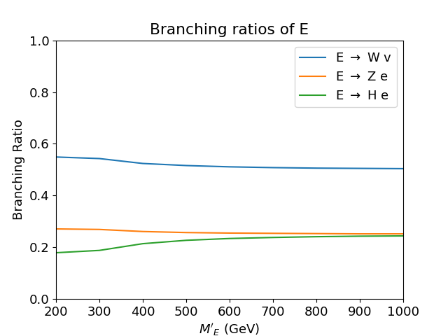
Figure 1: Branching ratios of the $SU(2)$ singlet $E$ as a function of the mass parameter $M^{\prime}_{E}$.

Together, these lead to the following expressions for the partial decay widths of the mass eigenstate $E$:

$$\Gamma(E\rightarrow Ze) =\frac{s^{2}_{L}c^{2}_{L}}{32\pi}\frac{M^{{}^{\prime}3}_{E}}{v^{2}}\left(1-\frac{M^{2}_{Z}}{M^{{}^{\prime}2}_{E}}\right)^{2}\left(1+2\frac{M^{2}_{Z}}{M^{{}^{\prime}2}_{E}}\right)$$ (8)

$$\Gamma(E\rightarrow he) =\frac{\lambda^{2}_{E}M^{\prime}_{E}c^{2}_{L}c^{2}_{R}}{64\pi}\left(1-\frac{M^{2}_{H}}{M^{{}^{\prime}2}_{E}}\right)^{2}$$ (9)

$$\Gamma(E\rightarrow W\nu_{e}) =\frac{s^{2}_{L}}{16\pi}\frac{M^{{}^{\prime}3}_{E}}{v^{2}}\left(1-\frac{M^{2}_{W}}{M^{{}^{\prime}2}_{E}}\right)^{2}\left(1+2\frac{M^{2}_{W}}{M^{{}^{\prime}2}_{E}}\right)$$ (10)

The branching ratios are plotted in Figure 1, which can be seen to evince the Goldstone equivalence theorem for large $M^{\prime}_{E}$. Note that in the regime where $\frac{\lambda_{E}v}{M^{\prime}_{E}}\ll 1$ all the decay widths have the same dependence on $\lambda_{E}$, so the branching ratios will be independent of its value.

In this region of parameter space, the Drell-Yan-like double production through the gauge coupling is significantly larger than single production rates, so we restrict our attention to that mode. We note that this means our cross-section for on-shell production followed by decay into at least one Higgs is independent of the Yukawa coupling. To calculate cross sections at the LHC, we implement the model in FeynRules [79] as input to MadGraph 5 [80] for Monte Carlo simulation. We plot the production cross section as a function of $M^{\prime}_{E}$ in Figure 2 and note that we are in agreement with [81].

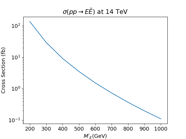
Figure 2: Production cross section of $E\bar{E}$ at the $14$ TeV LHC.

In Section III we will study the constraints on this model from Run 2 of the LHC and compare the prospects for BSM Higgs production, but for now we will proceed to discuss the next representation.

II.2 The Doublet

Next on the list, we consider a vector-like SU(2) doublet $\Delta_{1}$, transforming as $(1,2,-\frac{1}{2})$, with its partner $\bar{\Delta}_{1}$ [53]. After EWSB we’ll find we have one neutral field and one charged field, so we denote the corresponding left-handed Weyl fields:

$$\Delta_{1} =\begin{bmatrix}N\\ E\end{bmatrix},$$ (11)

and similarly for $\bar{\Delta}_{1}$. Since we have a vector-like pair, a mass term is allowed in the Lagrangian.

Such doublets are required in certain grand unification schemes (e.g. $E_{6}$ [82, 83]) or may appear simply as the supersymmetric partners of the two Higgs doublets in the MSSM, with $\Delta_{1}\simeq\tilde{H}_{u},\bar{\Delta}_{1}\simeq\tilde{H}_{d}$.

Before electroweak symmetry breaking, the allowed Yukawa interaction can be written as:

$$\mathcal{L}_{\text{Yuk}}=-\lambda_{\Delta_{1}}\bar{\Delta}_{1}\phi\bar{e}+h.c.$$ (12)

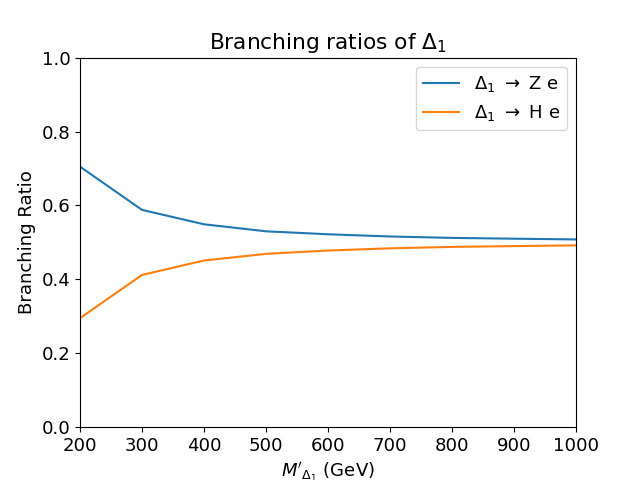
Figure 3: Branching ratios of the charged component of the $SU(2)$ doublet $\Delta_{1}$ as a function of the mass parameter $M^{\prime}_{\Delta_{1}}$.

Unlike the previous case the coupling is now to the right-handed electron. This interaction leads to mixing solely for the charged component $E$.

The gauge interaction terms are now:

$$\mathcal{L}_{\text{Gauge}} =\frac{g_{2}}{\sqrt{2}}W^{+}_{\mu}N^{\dagger}\bar{\sigma}^{\mu}E$$

$$+\frac{g_{2}}{c_{w}}Z_{\mu}\left(-\frac{1}{2}+s^{2}_{w}\right)E^{\dagger}\bar{\sigma}^{\mu}E$$

$$+\frac{g_{2}}{2c_{w}}Z_{\mu}N^{\dagger}\bar{\sigma}^{\mu}N$$

$$+eA_{\mu}E^{\dagger}\bar{\sigma}^{\mu}E,$$ (13)

where there are additional similar terms for the right handed fields $\bar{E},\bar{N}$. The mass matrix in this case is given by:

$$\mathcal{M}_{\Delta}=\begin{pmatrix}m^{\prime}_{E}&0\\ \frac{\lambda_{\Delta_{1}}v}{\sqrt{2}}&M^{\prime}_{\Delta_{1}}\end{pmatrix}$$ (14)

As before, the parameter $m^{\prime}_{E}$ must be chosen to ensure the lighter eigenvalue of $\mathcal{M}_{\Delta}^{2}$ corresponds to the physical electron mass $m_{e}$. We repeat the same procedure as above and find the eigenvalues similarly:

$$m_{e}=m^{\prime}_{E}\left(1-\frac{\lambda_{E}^{2}v^{2}}{4M^{{}^{\prime}2}_{\Delta_{1}}}\right),\quad M_{\Delta_{1}}=M^{\prime}_{\Delta_{1}}\left(1+\frac{\lambda^{2}_{\Delta_{1}}v^{2}}{4M^{{}^{\prime}2}_{\Delta_{1}}}\right).$$ (15)

As for the mass eigenstates, this time the mixing angles to first order in $\lambda_{\Delta_{1}}$ are:

$$\theta_{R}=\frac{\lambda_{\Delta_{1}}v}{\sqrt{2}M^{\prime}_{\Delta_{1}}},\qquad\theta_{L}=-\frac{\lambda_{\Delta_{1}}v}{\sqrt{2}M^{\prime}_{\Delta_{1}}}\frac{m_{e}}{M^{\prime}_{\Delta_{1}}},$$ (16)

with now the left-handed mixing being suppressed by a mass insertion. Using the previous convention for compactifying the mixing angle expressions, we expand the gauge interaction terms in terms of mass eigenstates to first order, and we find the mixed gauge interaction terms in the mass basis:

$$\mathcal{L}_{\text{Gauge}}\supset-\frac{g_{2}}{2c_{w}}s_{R}c_{R}\bar{E}^{\dagger}\bar{\sigma}^{\mu}Z_{\mu}\bar{e}-\frac{g_{2}}{\sqrt{2}}s_{R}W^{+}_{\mu}\bar{N}\sigma^{\mu}\bar{e}^{\dagger}+h.c.,$$ (17)

with the photon vertex cancelling out.

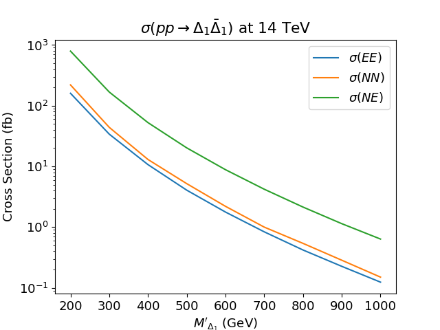
Figure 4: Production cross section of the components of $\Delta_{1}\bar{\Delta}_{1}$ at the 14 TeV LHC.

We can now calculate decay widths for the mass eigenstates $E$, $N$, which we find to be:

$$\Gamma(E\rightarrow Ze)=\frac{s^{2}_{R}c^{2}_{R}}{32\pi}\frac{M^{{}^{\prime}3}_{\Delta_{1}}}{v^{2}}\left(1-\frac{M^{2}_{Z}}{M^{{}^{\prime}2}_{\Delta_{1}}}\right)^{2}\left(1+2\frac{M^{2}_{Z}}{M^{{}^{\prime}2}_{\Delta_{1}}}\right)$$ (18)

$$\Gamma(E\rightarrow he)=\frac{\lambda^{2}_{\Delta_{1}}M^{\prime}_{\Delta_{1}}c^{2}_{L}c^{2}_{R}}{64\pi}\left(1-\frac{M^{2}_{H}}{M^{{}^{\prime}2}_{\Delta_{1}}}\right)^{2}$$ (19)

$$\Gamma(N\rightarrow We)=\frac{s^{2}_{R}}{16\pi}\frac{M^{{}^{\prime}3}_{\Delta_{1}}}{v^{2}}\left(1-\frac{M^{2}_{W}}{M^{{}^{\prime}2}_{\Delta_{1}}}\right)^{2}\left(1+2\frac{M^{2}_{W}}{M^{{}^{\prime}2}_{\Delta_{1}}}\right)$$ (20)

We plot the branching ratios of the charged component as a function of $M^{\prime}_{\Delta_{1}}$ in Figure 3.

We simulate the $pp\rightarrow\Delta_{1}\bar{\Delta}_{1}$ cross section in the same manner as above, and find the production cross sections in Figure 4, which are again in agreement with [81]. We note that $N$ decays solely to $We$ so its production does not lead to anomalous Higgs events.

We turn now to the final representation we study.

II.3 The Triplet

Finally, we consider a vector-like SU(2) triplet fermion with zero hypercharge, which we’ll denote by $\Sigma$ [53]. Such a field is familiar from, for example, type III Seesaw models [84], where neutrino mass originates through mixing with $\Sigma$.

We’ll find it convenient to regard the adjoint representation as the traceless bifundamental, so we represent $\Sigma$ as a $2\times 2$ matrix according to $\Sigma_{\alpha\bar{\alpha}}=\Sigma^{a}\sigma^{a}_{\alpha\bar{\alpha}}$, which we break into components as

$$\Sigma=\begin{pmatrix}N/\sqrt{2}&E^{+}\\ E^{-}&-N/\sqrt{2}\end{pmatrix}$$ (21)

The charged components may pair up to form a Dirac spinor, $\psi_{E}=\left(E^{-},(E^{+})^{\dagger}\right)^{\intercal}$, while we can write a Majorana spinor for the neutral component $\psi_{N}=\left(N,(N)^{\dagger}\right)^{\intercal}$.

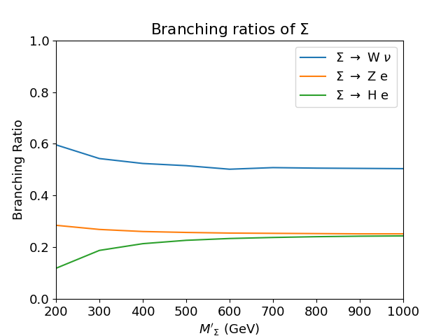
Figure 5: Branching ratios of the charged component of the $SU(2)$ triplet $\Sigma$ as a function of the mass parameter $M^{\prime}_{\Sigma}$.

The Yukawa interaction now looks like

$$\mathcal{L}_{\text{Yuk}}=-\lambda_{\Sigma}\tilde{\phi}^{\dagger}\Sigma L+h.c.$$ (22)

After EWSB this includes Yukawa interactions with both the left-handed electron and neutrino

$$\mathcal{L}_{\text{Yuk}}=-\frac{\lambda_{\Sigma}hN\nu_{e}}{2}+\frac{\lambda_{\Sigma}hE^{+}e}{\sqrt{2}}\ +\ h.c.$$ (23)

Expanding the covariant derivative, we find the gauge interaction terms:

$$\mathcal{L}_{\text{Gauge}} =g_{2}c_{w}E^{+}\sigma^{\mu}Z_{\mu}(E^{+})^{\dagger}+g_{2}c_{w}(E^{-})^{\dagger}\bar{\sigma}^{\mu}Z_{\mu}E^{-}$$

$$+eE^{+}\sigma^{\mu}A_{\mu}(E^{+})^{\dagger}+e(E^{-})^{\dagger}\bar{\sigma}^{\mu}A_{\mu}E^{-}$$ (24)

$$-g_{2}N\sigma^{\mu}W^{+}_{\mu}(E^{+})^{\dagger}-g_{2}N^{\dagger}\sigma^{\mu}W^{+}_{\mu}E^{-}+h.c.$$

This Yukawa interaction induces mixing of both the charged and neutral components of $\Sigma$ with SM leptons, so we now have two non-trivial mass matrices.

The charged mass matrix is given by:

$$\mathcal{M}=\begin{pmatrix}m^{\prime}_{E}&\frac{\lambda_{\Sigma}v}{\sqrt{2}}\\ 0&M^{\prime}_{\Sigma}\end{pmatrix},$$ (25)

and the Majorana mass matrix for the neutral states is:

$$\mathcal{M}_{0}=\begin{pmatrix}m^{\prime}_{\nu}&\frac{\lambda_{\Sigma}v}{2}\\ \frac{\lambda_{\Sigma}v}{2}&M^{\prime}_{\Sigma}\end{pmatrix}.$$ (26)

As we do not wish to specialize to type III seesaw models, we have included also a bare mass for the electron neutrino, $m^{\prime}_{\nu}$, so that we can study general mixing with $\Sigma$ while keeping the neutrino mass fixed, which we set to $50$ meV.

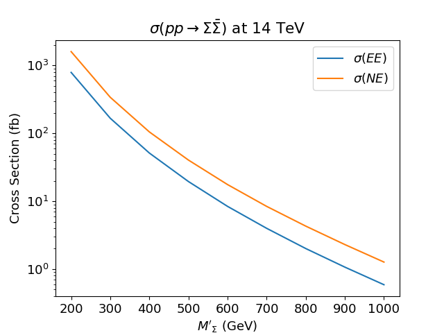
Figure 6: Production cross section of the components of $\Sigma\bar{\Sigma}$ at the $14$ TeV LHC.

As before, the lighter mass eigenstates, consisting primarily of the SM leptons, have their masses shifted down from the Lagrangian parameters

$$m_{e} =m^{\prime}_{E}\left(1-\frac{\lambda^{2}_{\Sigma}v^{2}}{4M^{{}^{\prime}2}_{\Sigma}}\right)$$ (27)

$$m_{\nu} =m^{\prime}_{\nu}-\frac{\lambda^{2}_{\Sigma}v^{2}}{4M^{\prime}_{\Sigma}},$$ (28)

and the heavier mass eigenvalues are likewise shifted up

$$M_{\Sigma^{\pm}} =M^{\prime}_{\Sigma}\left(1+\frac{\lambda^{2}_{\Sigma}v^{2}}{4M^{{}^{\prime}2}_{\Sigma}}\right)$$ (29)

$$M_{\Sigma^{0}} =M^{\prime}_{\Sigma}\left(1+\frac{\lambda^{2}_{\Sigma}v^{2}}{4M^{{}^{\prime}2}_{\Sigma}}\right),$$ (30)

where we note that this tree-level degeneracy will be broken by radiative corrections.

To diagonalize the charged mass matrix, we can repeat our procedure for the previous two cases and find

$$\theta_{L}=-\frac{\lambda_{\Sigma}v}{\sqrt{2}M^{\prime}_{\Sigma}},\qquad\theta_{R}=\frac{\lambda_{\Sigma}v}{\sqrt{2}M^{\prime}_{\Sigma}}\frac{m_{e}}{M^{\prime}_{\Sigma}},$$ (31)

and for the neutral mass matrix we only have a single mixing

$$\theta_{N}=\frac{\lambda_{\Sigma}v}{2M^{\prime}_{\Sigma}}.$$ (32)

Shifting now to the mass basis with the same conventions as above, we find mixed gauge interactions

$$\mathcal{L}_{\text{Gauge}} \supset g_{2}\left(c_{N}s_{L}-\frac{1}{\sqrt{2}}c_{R}s_{N}\right)N^{\dagger}W^{+}_{\mu}\bar{\sigma}^{\mu}e$$

$$-g_{2}s_{N}c_{R}(E^{+})^{\dagger}W^{+}_{\mu}\sigma^{\mu}\nu$$

$$+\frac{g_{2}}{2c_{w}}s_{N}c_{N}N^{\dagger}Z_{\mu}\sigma^{\mu}\nu$$

$$-\frac{g_{2}}{2c_{w}}s_{L}c_{R}(E^{-})^{\dagger}Z_{\mu}\sigma^{\mu}e.$$ (33)

From this we can simply compute the partial decays widths, which for the neutral component $N$ are:

$$\Gamma(N\rightarrow Z\nu) =\frac{s^{2}_{N}c^{2}_{N}}{32\pi}\frac{M^{{}^{\prime}3}_{\Sigma}}{v^{2}}\left(1-\frac{M^{2}_{Z}}{M^{{}^{\prime}2}_{\Sigma}}\right)^{2}\left(1+2\frac{M^{2}_{Z}}{M^{{}^{\prime}2}_{\Sigma}}\right)$$ (34)

$$\Gamma(N\rightarrow h\nu) =\frac{\lambda^{2}_{\Sigma}M^{\prime}_{\Sigma}c^{4}_{N}}{128\pi}\left(1-\frac{M^{2}_{H}}{M^{{}^{\prime}2}_{\Sigma}}\right)^{2}$$ (35)

$$\Gamma(N\rightarrow We) =\frac{(2c_{N}s_{L}-\sqrt{2}c_{R}s_{N})^{2}}{32\pi}\times$$ (36)

$$\frac{M^{{}^{\prime}3}_{\Sigma}}{v^{2}}\left(1-\frac{M^{2}_{W}}{M^{{}^{\prime}2}_{\Sigma}}\right)^{2}\left(1+2\frac{M^{2}_{W}}{M^{{}^{\prime}2}_{\Sigma}}\right).$$

And for the charged components $E^{\pm}$, the decay widths are:

$$\Gamma(E\rightarrow Ze) =\frac{s^{2}_{L}c^{2}_{L}}{32\pi}\frac{M^{{}^{\prime}3}_{\Sigma}}{v^{2}}\left(1-\frac{M^{2}_{Z}}{M^{{}^{\prime}2}_{\Sigma}}\right)^{2}\left(1+2\frac{M^{2}_{Z}}{M^{{}^{\prime}2}_{\Sigma}}\right)$$ (37)

$$\Gamma(E\rightarrow he) =\frac{\lambda^{2}_{\Sigma}M^{\prime}_{\Sigma}c^{2}_{L}c^{2}_{R}}{64\pi}\left(1-\frac{M^{2}_{H}}{M^{{}^{\prime}2}_{\Sigma}}\right)^{2}$$ (38)

$$\Gamma(E\rightarrow W\nu) =\frac{s^{2}_{N}c^{2}_{R}}{8\pi}\frac{M^{{}^{\prime}3}_{\Sigma}}{v^{2}}\times$$ (39)

$$\left(1-\frac{M^{2}_{W}}{M^{{}^{\prime}2}_{\Sigma}}\right)^{2}\left(1+2\frac{M^{2}_{W}}{M^{{}^{\prime}2}_{\Sigma}}\right).$$

We plot these branching ratios in Figure 5 and the double production cross section in Figure 6, finding agreement with [85]. With the stage now set, we turn to considering the constraints on these fields.

III Constraints and Discovery Potential

As mentioned above, low-energy constraints on SMEFT operators can be straightforwardly used to constrain the presence of new BSM states. For many single field extensions the constraints have been systematically studied and Ref. [52] gives bounds in the $(\lambda_{i},M^{\prime}_{i})$ parameter space for our three representations which we reproduce in Table 1.

Table 1: Constraints from the SMEFT Analysis [52].

E	$\Delta_{1}$	$\Sigma$
$\frac{\lambda^{2}_{E}}{M^{{}^{\prime}2}_{E}}\leq\frac{2.1\times 10^{-2}}{1\text{ TeV}^{2}}$	$\frac{\lambda^{2}_{\Delta_{1}}}{M^{{}^{\prime}2}_{\Delta_{1}}}\leq\frac{1.7\times 10^{-2}}{1\text{ TeV}^{2}}$	$\frac{\lambda^{2}_{\Sigma}}{M^{{}^{\prime}2}_{\Sigma}}\leq\frac{4.5\times 10^{-2}}{1\text{ TeV}^{2}}$

At the energy frontier, the best constraints on these models come from multilepton searches. Such searches, which require 3 or more final state leptons, essentially look for the decay modes to $W$ or $Z$ and their leptonic decays. There are thus large penalties from the high branching ratios to jets or neutrinos. The strongest constraint comes from the 13 TeV CMS multilepton search [73] taking advantage of the full Run 2 data set. The CMS analysis interprets the search in the context of a type III seesaw model with flavor-democratic couplings, and we use this model to validate our reinterpretation procedure. Details on the procedure and the validation are given in the appendix. For completeness we mention the ATLAS Run 2 dilepton + jets search [86], which interprets their search with the same signal model and finds a bound which is nearly as strong, but we below reinterpret solely the leading bound from CMS. For earlier work related to bounds on the production of general vector-like leptons at colliders, see e.g. [87, 88, 89, 90, 91, 92, 93, 94] and [95, 85, 96, 97, 98, 99, 100, 101, 102, 103, 104, 105, 106, 107, 108, 109, 110]

After Monto Carlo simulation from MadGraph 5 we put the events through Pythia [111] for decays and showering and then Delphes [112] for detector simulation. Then we pass the resulting .lhco files through our reinterpretation of the CMS analysis using MadAnalysis [113] and translate our results into bounds on the mass parameter. We derive the 95% confidence lower bounds for each field that are shown in Table 2.

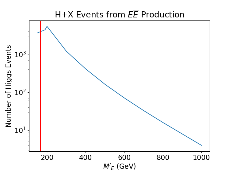
Figure 7: Number of anomalous Higgs events from production of the $SU(2)$ Singlet at Run 2 of the LHC. The red line denotes the lower mass bound placed by our reinterpretation of the CMS multilepton search.

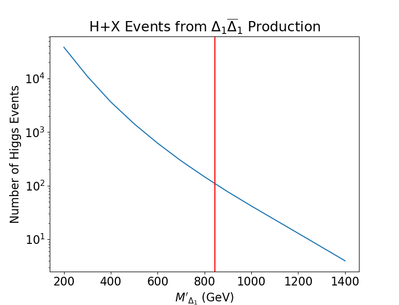
Figure 8: The same as Figure 7 for the doublet.

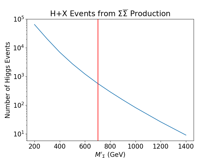
Figure 9: The same as Figure 7 for the triplet.

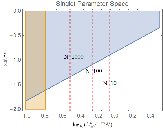
Figure 10: Bounds on the singlet parameter space from the SMEFT analysis [52] (blue) and the CMS multilepton search [73] (orange). The dashed lines show the masses at which the labeled number of anomalous Higgs events would have been produced in Run 2.

Figure 11: The same as Figure 10 for the doublet.

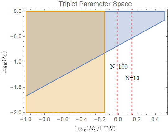
Figure 12: The same as Figure 10 for the triplet.

As discussed in Section I, our newfound adeptness at identifying Higgs decays makes the Higgs itself a promising tagging object. To explore this, we study the pair production of our heavy leptons which include at least one decay to Higgs + X. While we do not attempt to mock up a realistic search, we will show that there is ample parameter space which the multilepton searches are unable to probe, yet which lead to a large rate of exotic Higgs production events. In Figures 7, 8, 9 we plot the number of anomalous Higgs events each model would have produced in Run 2 of the LHC as a function of the mass of the new lepton. In Figures 10, 11, 12 we show the constraints on these three models from the SMEFT analysis and our reinterpretation of the CMS multilepton search.

Table 2: Bounds from the 13 TeV CMS Multilepton Search

E	$\Delta_{1}$	$\Sigma$
$M^{\prime}_{E}>167\text{ GeV}$	$M^{\prime}_{\Delta_{1}}>844\text{ GeV}$	$M^{\prime}_{\Sigma}>705\text{ GeV}$

As can be seen for the singlet from Figure 7, there are an abundance of exotic Higgs production events beyond where the Run 2 leptonic searches impose a bound. Figure 10 illustrates for the same model how BSM Higgs production compares to bounds from SMEFT and the CMS multilepton search.

We note again that in calculating the numbers of Higgs produced we use the branching ratios at $\lambda v/M^{\prime}_{E}\ll 1$, which are independent of the value of $\lambda$. This is satisfied everywhere in the parameter space which is not already ruled out by SMEFT constraints. Resultingly we do not worry about the precise shape of the constraint from multilepton searches in the $\lambda v/M^{\prime}_{E}\sim 1$ regime, which would solely modify the upper left corner of Figure 10.

The analogous results for the doublet and triplet may be found in Figures 8, 11 and 9, 12, respectively. As evinced by these plots, there is a significant number of anomalous Higgs events produced outside of the region in parameter space ruled out by SMEFT bounds and current LHC searches. The benefit of a search for anomalous Higgs decays is most clear in the case of the singlet, but if a search can be designed with few background events, it should be able to probe untouched parameter space in all three models. The presence of resonances in 2- and 3-body invariant mass spectra should help make such a possibility practicable.

IV Conclusion

The LHC is likely to be our clearest window into the energy frontier of the electroweak sector for at least the next couple decades. Obviously, we must wring every bit of constraining power out of the data we collect at the experiments. While the data can be fully analyzed at our leisure over the years when future machines are being built, the data collection itself confers urgency due to our finite capacity for processing and storing events. Over the next years, the LHC will deliver what is likely the last 14 TeV proton-proton collisions that humanity has access to for hundreds of years, if not far longer. Each event in every inverse femtobarn of integrated luminosity which is not written to tape is an event which is lost forever to time, so we had better be damn sure we’re keeping the right ones. Note particularly that a 100 TeV collider this century will not necessarily be able to make up this lost opportunity—data at different center-of-mass energies are complementary, and indeed data from the Tevatron has still been useful in the LHC era. So understanding the optimal signatures and triggers and searches to use to look for new physics is absolutely critical, as well as pressing.

While the wide range of possible models of the universe makes systematically searching for new physics a cumbersome task, we have focused on a well-motivated restricted catalog of new fields to look for at a collider. We have argued that searches for signatures from the decays of on-shell new physics into Higgses can have greater reach than those currently performed toward the goal of probing new particles with SM charges. This can be motivated by quite general arguments for new massive color singlets with electroweak charges, for which the numbers of decays to Higgses and gauge bosons are similar. We have then evinced the opportunities available for such searches by reinterpreting current searches for the best bounds on a few representative new species, and showing that despite current constraints we may be allowing an enormous number of exotic Higgs production events to go unnoticed. This indicates that implementing a search for these Higgs + X final states may be able to improve the existing bounds on these models. Explicitly constructing such a search strategy we leave to the experimentalists.

Of course there remains much more to be explored. We have not gone through each possibility in the catalog of interesting single-field extensions, particularly in restricting our attention to fermions in vector-like representations which couple to first-generation leptons. Furthermore, our strategy of focusing on single-field extensions is convenient in providing a simple, manageable catalog, but the extension of the SM chosen by Nature may well have multiple new particles within reach of the energy frontier. One could imagine a wider array of phenomenologies when there is not a large gap between the lightest new state and the second-lightest. Mapping out the possibilities with two new states may be useful for pointing out in which regions of parameter space there are other signatures, not appearing in single-field extensions, that become the best way to constrain them. This may be a collider search for different final states, or displaced decays appearing when the states are nearly degenerate, or signals appearing in tabletop experiments or cosmological observations or elsewhere.

The other clear direction of generalization is to study the production of and potential searches for species whose decays include other final states along with Higgses. While our focus has been on the electroweak energy frontier, analogous benefits may come from looking for decays of new colored fields to Higgses and jets, as has already been usefully done for e.g. vector-like quarks [114, 115]. Furthermore, three-body decays through effective five-dimensional operators including Higgses can be phenomenologically relevant in a variety of theories, from weak scale supersymmetry (e.g. [116, 117]) to theories with exotic representations (e.g. [118, 119]), and motivate looking for new particles decaying to, for example, $H+q\bar{q}$ or $H+\ell\ell$. It is more than worth understanding all the channels in which searches for final states with Higgs resonances may improve our coverage.

Despite our hopes and expectations, new physics has proven hard to find at the LHC. We hit paydirt with the discovery of the Higgs, but our intellectual curiosity is far from sated and drives us to continue digging. Looking throughout the parameter space of expected signals remains useful, and the fantastic constraints already placed on many, many models are a testament to experimental efforts. We have here suggested a new search strategy for electroweak states which makes fundamental use of our most recent, exciting discovery. How elegant it would be for Higgs resonances to once more lead us to the next great treasure of particle physics.

*

Appendix A CMS Multilepton Search Reinterpretation

The most stringent constraints on these models from the LHC come from searches for multilepton final states. We reinterpeted the 13 TeV CMS search [73] with $137\text{ fb}^{-1}$ of data using expert mode of MadAnalysis 5 [113] to implement cuts and event selection. We simulated events in MadGraph 5, passed them to Pythia for decays and showering, and then to Delphes for detector simulation. The cuts and event selection of the type-III seesaw signal regions were implemented faithfully, except that the impact parameter requirements were ignored. We found that it was crucial to use the same PDF as the CMS analysis, namely NNPDF3.0 (LHAPDF ID: 261000) as described in [120]. Another important ingredient was the lepton reconstruction efficiency, for which we could not find exact specifications. We based our electron and muon efficiencies mainly on [121] and [122] respectively, and implemented them as shown in Figures 13, 14.

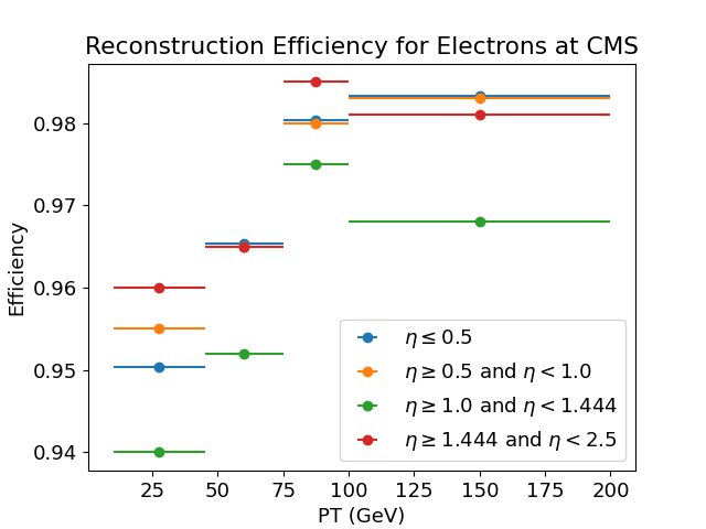
Figure 13: The Electron Identification Efficiency we use for the Delphes Card.

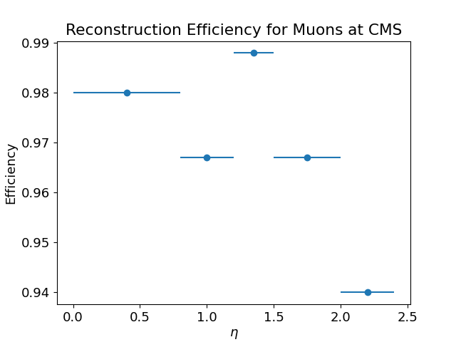
Figure 14: The Muon Identification Efficiency we use for the Delphes Card.

To validate our reinterpretation, we simulated 100k $pp\rightarrow\Sigma\bar{\Sigma}$ events in the Type-III flavor democratic seesaw model for which the CMS analysis [73] presents simulation results. In Figures 15-21 we compare the results of our simulation and reinterpretation to those of CMS for the parameter point $M_{\Sigma}=700\text{ GeV}$.

After validating our simulation and reinterpretation pipeline, we derive upper limits at 95% confidence level on the number of signal events in any signal region assuming Poisson distributions for the signal and background, and ignoring the uncertainty in the backgrounds. We use data found in the HEPData repository entry for this search. Lacking the full covariance matrix for the many signal regions, we instead conservatively say that a model point is ruled out at 95% confidence if it predicts more events than the 95% upper limit in any individual bin. As expected, the bins with the highest values of the kinematic discriminants tend to give the most stringent upper limits. The 95% confidence limits placed from this reinterpretation can be found in Table 2.

There are 7 exclusive signal regions of relevance for our reinterpretation of the CMS search. The events are first distinguished based on whether they contain 3 leptons (‘3L’) or at least 4 leptons (‘4L’). The events with 3 leptons are further divided into four distinct signal regions: those that have an opposite sign same flavor (OSSF) lepton pair with invariant mass below the ‘Z mass window’ $M_{Z}\pm 15\text{ GeV}$ (‘Below-Z’), those that have an OSSF pair within the Z mass window (‘On-Z’), that have an OSSF pair above the Z mass window (‘Above-Z’), and those with no OSSF pair at all (‘OSSF0’). The events with 4 or more leptons are similarly divided into regions that have 0, 1, and 2 OSSF pairs. The signal regions are then binned based on a kinematic discriminant variable $L_{T}+p_{T}^{\text{miss}}$, which is the scalar sum of the $p_{T}$ of all charged final state leptons plus the missing energy. However for the 3L On-Z region, an alternate kinematic discriminant is found to increase sensitivity, so $M_{T}=\sqrt{2p^{miss}_{T}p^{l}_{T}(1-\cos(\Delta\phi_{p^{miss}_{T},p^{l}_{T}}))}$ is used, where $p^{l}_{T}$ is the transverse momentum of the lepton which is not part of the OSSF pair.

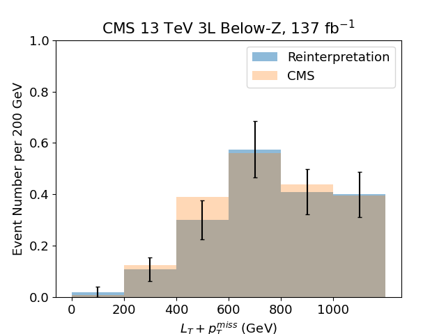
Figure 15: Comparison of the 3L below-Z signal region between the simulation performed in the CMS analysis [73] for the $M_{\Sigma}=700\text{ GeV}$ point and our simulation of the same model implemented in our analysis pipeline. The black intervals denote our $1\sigma$ statistical uncertainty bands.

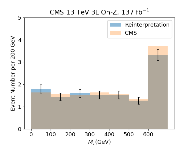
Figure 16: The same as Figure 15 for the 3L on-Z signal region.

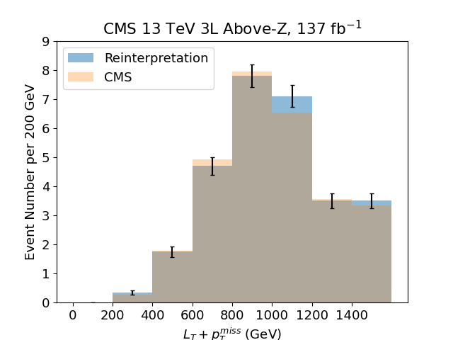
Figure 17: The same as Figure 15 for the 3L above-Z signal region.

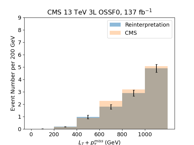
Figure 18: The same as Figure 15 for the 3L OSSF0 signal region.

Figure 19: The same as Figure 15 for the 4L OSSF0 signal region.

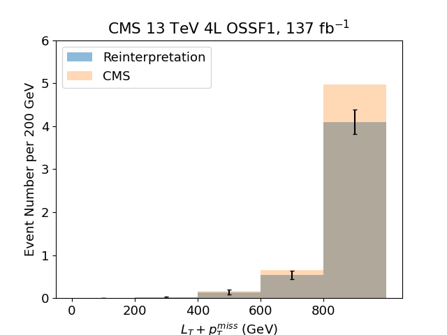
Figure 20: The same as Figure 15 for the 4L OSSF1 signal region.

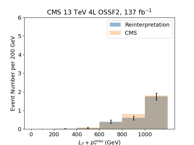
Figure 21: The same as Figure 15 for the 4L OSSF2 signal region.

References

- Aad et al. [2012] G. Aad, T. Abajyan, B. Abbott, J. Abdallah, S. Abdel Khalek, A. Abdelalim, O. Abdinov, R. Aben, B. Abi, M. Abolins, and et al., Observation of a new particle in the search for the standard model higgs boson with the atlas detector at the lhc, Physics Letters B 716, 1–29 (2012).
- Chatrchyan et al. [2012a] S. Chatrchyan, V. Khachatryan, A. Sirunyan, A. Tumasyan, W. Adam, E. Aguilo, T. Bergauer, M. Dragicevic, J. Erö, C. Fabjan, and et al., Observation of a new boson at a mass of 125 gev with the cms experiment at the lhc, Physics Letters B 716, 30–61 (2012a).
- Kanemura et al. [2013] S. Kanemura, M. Kikuchi, and K. Yagyu, Probing exotic higgs sectors from the precise measurement of higgs boson couplings, Physical Review D 88, 015020 (2013).
- Cheung et al. [2013] K. Cheung, J. S. Lee, and P.-Y. Tseng, Higgs precision (higgcision) era begins, Journal of High Energy Physics 2013, 134 (2013).
- Carena et al. [2015] M. Carena, H. E. Haber, I. Low, N. R. Shah, and C. E. M. Wagner, Complementarity between Nonstandard Higgs Boson Searches and Precision Higgs Boson Measurements in the MSSM, Phys. Rev. D 91, 035003 (2015), arXiv:1410.4969 [hep-ph] .
- Henning et al. [2014] B. Henning, X. Lu, and H. Murayama, What do precision higgs measurements buy us? (2014), arXiv:1404.1058 [hep-ph] .
- Chen et al. [2017] X. Chen, Y. Wang, and Z.-Z. Xianyu, Standard Model Mass Spectrum in Inflationary Universe, JHEP 04, 058, arXiv:1612.08122 [hep-th] .
- East et al. [2017] W. E. East, J. Kearney, B. Shakya, H. Yoo, and K. M. Zurek, Spacetime Dynamics of a Higgs Vacuum Instability During Inflation, Phys. Rev. D 95, 023526 (2017), arXiv:1607.00381 [hep-ph] .
- Kumar and Sundrum [2018] S. Kumar and R. Sundrum, Heavy-Lifting of Gauge Theories By Cosmic Inflation, JHEP 05, 011, arXiv:1711.03988 [hep-ph] .
- Hook et al. [2020] A. Hook, J. Huang, and D. Racco, Searches for other vacua. Part II. A new Higgstory at the cosmological collider, JHEP 01, 105, arXiv:1907.10624 [hep-ph] .
- Huber and Konstandin [2008] S. J. Huber and T. Konstandin, Gravitational Wave Production by Collisions: More Bubbles, JCAP 09, 022, arXiv:0806.1828 [hep-ph] .
- Caprini et al. [2009] C. Caprini, R. Durrer, and G. Servant, The stochastic gravitational wave background from turbulence and magnetic fields generated by a first-order phase transition, JCAP 12, 024, arXiv:0909.0622 [astro-ph.CO] .
- Espinosa et al. [2010] J. R. Espinosa, T. Konstandin, J. M. No, and G. Servant, Energy Budget of Cosmological First-order Phase Transitions, JCAP 06, 028, arXiv:1004.4187 [hep-ph] .
- No [2011] J. M. No, Large gravitational wave background signals in electroweak baryogenesis scenarios, Physical Review D 84, 124025 (2011).
- Eboli and Zeppenfeld [2000] O. J. Eboli and D. Zeppenfeld, Observing an invisible higgs boson, Physics Letters B 495, 147 (2000).
- Bai et al. [2012] Y. Bai, P. Draper, and J. Shelton, Measuring the invisible higgs width at the 7 and 8 tev lhc, Journal of High Energy Physics 2012, 192 (2012).
- Ghosh et al. [2013] D. Ghosh, R. Godbole, M. Guchait, K. Mohan, and D. Sengupta, Looking for an Invisible Higgs Signal at the LHC, Phys. Lett. B 725, 344 (2013), arXiv:1211.7015 [hep-ph] .
- Belanger et al. [2013] G. Belanger, B. Dumont, U. Ellwanger, J. Gunion, and S. Kraml, Status of invisible Higgs decays, Phys. Lett. B 723, 340 (2013), arXiv:1302.5694 [hep-ph] .
- Strassler and Zurek [2007] M. J. Strassler and K. M. Zurek, Echoes of a hidden valley at hadron colliders, Physics Letters B 651, 374–379 (2007).
- Strassler and Zurek [2008] M. J. Strassler and K. M. Zurek, Discovering the higgs through highly-displaced vertices, Physics Letters B 661, 263–267 (2008).
- Curtin et al. [2014] D. Curtin et al., Exotic decays of the 125 GeV Higgs boson, Phys. Rev. D 90, 075004 (2014), arXiv:1312.4992 [hep-ph] .
- Curtin and Verhaaren [2015] D. Curtin and C. B. Verhaaren, Discovering Uncolored Naturalness in Exotic Higgs Decays, JHEP 12, 072, arXiv:1506.06141 [hep-ph] .
- Clarke [2015] J. D. Clarke, Constraining portals with displaced Higgs decay searches at the LHC, JHEP 10, 061, arXiv:1505.00063 [hep-ph] .
- Csaki et al. [2015] C. Csaki, E. Kuflik, S. Lombardo, and O. Slone, Searching for displaced Higgs boson decays, Phys. Rev. D 92, 073008 (2015), arXiv:1508.01522 [hep-ph] .
- Alipour-Fard et al. [2019] S. Alipour-Fard, N. Craig, M. Jiang, and S. Koren, Long Live the Higgs Factory: Higgs Decays to Long-Lived Particles at Future Lepton Colliders, Chin. Phys. C 43, 053101 (2019), arXiv:1812.05588 [hep-ph] .
- Cheung and Wang [2020] K. Cheung and Z. S. Wang, Probing Long-lived Particles at Higgs Factories, Phys. Rev. D 101, 035003 (2020), arXiv:1911.08721 [hep-ph] .
- Fuchs et al. [2020] E. Fuchs, O. Matsedonskyi, I. Savoray, and M. Schlaffer, Collider searches of scalar singlets across lifetimes (2020), arXiv:2008.12773 [hep-ph] .
- Abachi et al. [1995] S. Abachi et al. (D0), Observation of the top quark, Phys. Rev. Lett. 74, 2632 (1995), arXiv:hep-ex/9503003 .
- Abe et al. [1995] F. Abe et al. (CDF), Observation of top quark production in collisions, Phys. Rev. Lett. 74, 2626 (1995), arXiv:hep-ex/9503002 .
- Baer et al. [2012] H. Baer, V. Barger, A. Lessa, W. Sreethawong, and X. Tata, Wh plus missing- signature from gaugino pair production at the LHC, Phys. Rev. D 85, 055022 (2012), arXiv:1201.2949 [hep-ph] .
- Howe and Saraswat [2012] K. Howe and P. Saraswat, Excess Higgs Production in Neutralino Decays, JHEP 10, 065, arXiv:1208.1542 [hep-ph] .
- Ghosh et al. [2012] D. Ghosh, M. Guchait, and D. Sengupta, Higgs Signal in Chargino-Neutralino Production at the LHC, Eur. Phys. J. C 72, 2141 (2012), arXiv:1202.4937 [hep-ph] .
- Arbey et al. [2015] A. Arbey, M. Battaglia, and F. Mahmoudi, Higgs Production in Neutralino Decays in the MSSM - The LHC and a Future Collider, Eur. Phys. J. C 75, 108 (2015), arXiv:1212.6865 [hep-ph] .
- Bharucha et al. [2013] A. Bharucha, S. Heinemeyer, and F. von der Pahlen, Direct Chargino-Neutralino Production at the LHC: Interpreting the Exclusion Limits in the Complex MSSM, Eur. Phys. J. C 73, 2629 (2013), arXiv:1307.4237 [hep-ph] .
- Han et al. [2013] T. Han, S. Padhi, and S. Su, Electroweakinos in the Light of the Higgs Boson, Phys. Rev. D 88, 115010 (2013), arXiv:1309.5966 [hep-ph] .
- Papaefstathiou et al. [2014] A. Papaefstathiou, K. Sakurai, and M. Takeuchi, Higgs boson to di-tau channel in Chargino-Neutralino searches at the LHC, JHEP 08, 176, arXiv:1404.1077 [hep-ph] .
- Ellwanger and Teixeira [2015] U. Ellwanger and A. M. Teixeira, Excessive Higgs pair production with little MET from squarks and gluinos in the NMSSM, JHEP 04, 172, arXiv:1412.6394 [hep-ph] .
- Zhang [2015] M. Zhang, The Heavy Higgs Decay Effect and Its Impact on Higgs Data Fitting in NMSSM (2015), arXiv:1505.05636 [hep-ph] .
- Chakraborti et al. [2015] M. Chakraborti, U. Chattopadhyay, A. Choudhury, A. Datta, and S. Poddar, Reduced LHC constraints for higgsino-like heavier electroweakinos, JHEP 11, 050, arXiv:1507.01395 [hep-ph] .
- Choudhury and Mondal [2016] A. Choudhury and S. Mondal, Revisiting the Exclusion Limits from Direct Chargino-Neutralino Production at the LHC, Phys. Rev. D 94, 055024 (2016), arXiv:1603.05502 [hep-ph] .
- Liu et al. [2020a] J. Liu, N. McGinnis, C. E. M. Wagner, and X.-P. Wang, The scale of superpartner masses and electroweakino searches at the high-luminosity LHC, JHEP 12, 087, arXiv:2008.11847 [hep-ph] .
- Liu et al. [2020b] J. Liu, N. McGinnis, C. E. M. Wagner, and X.-P. Wang, Searching for the Higgsino-Bino Sector at the LHC, JHEP 09, 073, arXiv:2006.07389 [hep-ph] .
- Kling et al. [2015] F. Kling, A. Pyarelal, and S. Su, Light Charged Higgs Bosons to AW/HW via Top Decay, JHEP 11, 051, arXiv:1504.06624 [hep-ph] .
- Dermisek et al. [2016a] R. Dermisek, E. Lunghi, and S. Shin, New decay modes of heavy Higgs bosons in a two Higgs doublet model with vectorlike leptons, JHEP 05, 148, arXiv:1512.07837 [hep-ph] .
- Dermisek et al. [2016b] R. Dermisek, E. Lunghi, and S. Shin, New constraints and discovery potential for Higgs to Higgs cascade decays through vectorlike leptons, JHEP 10, 081, arXiv:1608.00662 [hep-ph] .
- Dermisek et al. [2020a] R. Dermisek, E. Lunghi, and S. Shin, Cascade decays of heavy Higgs bosons through vectorlike quarks in two Higgs doublet models, JHEP 03, 029, arXiv:1907.07188 [hep-ph] .
- Dermíšek et al. [2019] R. Dermíšek, E. Lunghi, and S. Shin, Hunting for Vectorlike Quarks, JHEP 04, 019, [Erratum: JHEP 10, 058 (2020)], arXiv:1901.03709 [hep-ph] .
- Dermisek et al. [2020b] R. Dermisek, E. Lunghi, N. McGinnis, and S. Shin, Signals with six bottom quarks for charged and neutral Higgs bosons, JHEP 07, 241, arXiv:2005.07222 [hep-ph] .
- Kribs et al. [2010a] G. D. Kribs, A. Martin, T. S. Roy, and M. Spannowsky, Discovering the Higgs Boson in New Physics Events using Jet Substructure, Phys. Rev. D 81, 111501 (2010a), arXiv:0912.4731 [hep-ph] .
- Kribs et al. [2010b] G. D. Kribs, A. Martin, T. S. Roy, and M. Spannowsky, Discovering Higgs Bosons of the MSSM using Jet Substructure, Phys. Rev. D 82, 095012 (2010b), arXiv:1006.1656 [hep-ph] .
- Yu [2014] F. Yu, Anatomizing Exotic Production of the Higgs Boson, Phys. Rev. D 90, 015009 (2014), arXiv:1404.2924 [hep-ph] .
- Ellis et al. [2018] J. Ellis, C. W. Murphy, V. Sanz, and T. You, Updated global SMEFT fit to Higgs, diboson and electroweak data, Journal of High Energy Physics 2018, 10.1007/jhep06(2018)146 (2018).
- de Blas et al. [2018] J. de Blas, J. C. Criado, M. Pérez-Victoria, and J. Santiago, Effective description of general extensions of the Standard Model: the complete tree-level dictionary, Journal of High Energy Physics 2018, 10.1007/jhep03(2018)109 (2018).
- Han et al. [2021] T. Han, D. Liu, I. Low, and X. Wang, Electroweak Couplings of the Higgs Boson at a multi-TeV Muon Collider (2021).
- Han et al. [2020a] T. Han, Y. Ma, and K. Xie, High Energy Leptonic Collisions and Electroweak Parton Distribution Functions (2020a), arXiv:2007.14300 [hep-ph] .
- Han et al. [2020b] T. Han, Z. Liu, L.-T. Wang, and X. Wang, WIMPs at High Energy Muon Colliders (2020b), arXiv:2009.11287 [hep-ph] .
- Chiesa et al. [2020] M. Chiesa, F. Maltoni, L. Mantani, B. Mele, F. Piccinini, and X. Zhao, Measuring the quartic Higgs self-coupling at a multi-TeV muon collider, JHEP 09, 098, arXiv:2003.13628 [hep-ph] .
- Capdevilla et al. [2020] R. Capdevilla, D. Curtin, Y. Kahn, and G. Krnjaic, A Guaranteed Discovery at Future Muon Colliders (2020), arXiv:2006.16277 [hep-ph] .
- Costantini et al. [2020] A. Costantini, F. De Lillo, F. Maltoni, L. Mantani, O. Mattelaer, R. Ruiz, and X. Zhao, Vector boson fusion at multi-TeV muon colliders, JHEP 09, 080, arXiv:2005.10289 [hep-ph] .
- Yin and Yamaguchi [2020] W. Yin and M. Yamaguchi, Muon at multi-TeV muon collider (2020), arXiv:2012.03928 [hep-ph] .
- Buttazzo and Paradisi [2020] D. Buttazzo and P. Paradisi, Probing the muon g-2 anomaly at a Muon Collider (2020), arXiv:2012.02769 [hep-ph] .
- Capdevilla et al. [2021] R. Capdevilla, D. Curtin, Y. Kahn, and G. Krnjaic, A No-Lose Theorem for Discovering the New Physics of at Muon Colliders (2021), arXiv:2101.10334 [hep-ph] .
- Liu and Xie [2021] W. Liu and K.-P. Xie, Probing electroweak phase transition with multi-TeV muon colliders and gravitational waves (2021), arXiv:2101.10469 [hep-ph] .
- Bogomilov et al. [2020] M. Bogomilov et al. (MICE), Demonstration of cooling by the Muon Ionization Cooling Experiment, Nature 578, 53 (2020), arXiv:1907.08562 [physics.acc-ph] .
- Delahaye et al. [2019] J. P. Delahaye, M. Diemoz, K. Long, B. Mansoulié, N. Pastrone, L. Rivkin, D. Schulte, A. Skrinsky, and A. Wulzer, Muon Colliders (2019), arXiv:1901.06150 [physics.acc-ph] .
- Long et al. [2020] K. Long, D. Lucchesi, M. Palmer, N. Pastrone, D. Schulte, and V. Shiltsev, Muon Colliders: Opening New Horizons for Particle Physics (2020), arXiv:2007.15684 [physics.acc-ph] .
- Bartosik et al. [2020] N. Bartosik et al., Detector and Physics Performance at a Muon Collider, JINST 15 (05), P05001, arXiv:2001.04431 [hep-ex] .
- Burdman et al. [2007] G. Burdman, Z. Chacko, H.-S. Goh, and R. Harnik, Folded supersymmetry and the LEP paradox, JHEP 02, 009, arXiv:hep-ph/0609152 .
- Cai et al. [2009] H. Cai, H.-C. Cheng, and J. Terning, A Quirky Little Higgs Model, JHEP 05, 045, arXiv:0812.0843 [hep-ph] .
- Burdman et al. [2015] G. Burdman, Z. Chacko, R. Harnik, L. de Lima, and C. B. Verhaaren, Colorless Top Partners, a 125 GeV Higgs, and the Limits on Naturalness, Phys. Rev. D 91, 055007 (2015), arXiv:1411.3310 [hep-ph] .
- Serra et al. [2019] J. Serra, S. Stelzl, R. Torre, and A. Weiler, Hypercharged Naturalness, JHEP 10, 060, arXiv:1905.02203 [hep-ph] .
- Koren [2020] S. Koren, The Hierarchy Problem: From the Fundamentals to the Frontiers, Ph.D. thesis, UC, Santa Barbara (2020), arXiv:2009.11870 [hep-ph] .
- Sirunyan et al. [2020] A. M. Sirunyan et al. (CMS), Search for Physics Beyond the Standard Model in Multilepton Final States in Proton-Proton Collisions at 13 TeV, JHEP 03, 051, arXiv:1911.04968 [hep-ex] .
- Brüning and Rossi [2015] O. Brüning and L. Rossi, eds., The High Luminosity Large Hadron Collider: the new machine for illuminating the mysteries of Universe, Vol. 24 (2015).
- Scherk and Schwarz [1979] J. Scherk and J. H. Schwarz, How to Get Masses from Extra Dimensions, Nucl. Phys. B 153, 61 (1979).
- Pomarol and Quiros [1998] A. Pomarol and M. Quiros, The Standard model from extra dimensions, Phys. Lett. B 438, 255 (1998), arXiv:hep-ph/9806263 .
- Howard E. Haber [2012] S. Y. C. Howard E. Haber, The Mathematics of Fermion Mass Diagonalization, Physics Letters B , 1–29 (2012).
- Haber [2020] H. E. Haber, A tale of three diagonalizations (2020), arXiv:2009.03990 [hep-ph] .
- Alloul et al. [2014] A. Alloul, N. D. Christensen, C. Degrande, C. Duhr, and B. Fuks, FeynRules 2.0 — A Complete Toolbox for Tree-Level Phenomenology, Computer Physics Communications 185, 2250–2300 (2014).
- Alwall et al. [2011] J. Alwall, M. Herquet, F. Maltoni, O. Mattelaer, and T. Stelzer, MadGraph 5: Going Beyond, Journal of High Energy Physics 2011, 10.1007/jhep06(2011)128 (2011).
- Kumar and Martin [2015a] N. Kumar and S. P. Martin, Vectorlike leptons at the Large Hadron Collider, Physical Review D 92, 10.1103/physrevd.92.115018 (2015a).
- Gursey et al. [1976] F. Gursey, P. Ramond, and P. Sikivie, A Universal Gauge Theory Model Based on E6, Phys. Lett. B 60, 177 (1976).
- Gursey and Serdaroglu [1978] F. Gursey and M. Serdaroglu, Basic Fermion Masses and Mixings in the Model, Lett. Nuovo Cim. 21, 28 (1978).
- Foot et al. [1989] R. Foot, H. Lew, X. He, and G. C. Joshi, Seesaw Neutrino Masses Induced by a Triplet of Leptons, Z. Phys. C 44, 441 (1989).
- Franceschini et al. [2008] R. Franceschini, T. Hambye, and A. Strumia, Type-iii seesaw mechanism at cern lhc, Physical Review D 78, 10.1103/physrevd.78.033002 (2008).
- Aad et al. [2020] G. Aad et al. (ATLAS), Search for type-III seesaw heavy leptons in dilepton final states in collisions at = 13 TeV with the ATLAS detector (2020), arXiv:2008.07949 [hep-ex] .
- Buskulic et al. [1996] D. Buskulic et al. (ALEPH), Search for heavy lepton pair production in e+ e- collisions at center-of-mass energies of 130-GeV and 136-GeV, Phys. Lett. B 384, 439 (1996).
- Ackerstaff et al. [1998] K. Ackerstaff et al. (OPAL), Search for stable and longlived massive charged particles in e+ e- collisions at s**(1/2) = 130-GeV - 183-GeV, Phys. Lett. B 433, 195 (1998), arXiv:hep-ex/9803026 .
- Abreu et al. [1999] P. Abreu et al. (DELPHI), Search for composite and exotic fermions at LEP-2, Eur. Phys. J. C 8, 41 (1999), arXiv:hep-ex/9811005 .
- Acciarri et al. [1999] M. Acciarri et al. (L3), Search for heavy neutral and charged leptons in annihilation at = 183-GeV and 189-GeV, Phys. Lett. B 462, 354 (1999), arXiv:hep-ex/9909007 .
- Achard et al. [2001] P. Achard et al. (L3), Search for heavy neutral and charged leptons in annihilation at LEP, Phys. Lett. B 517, 75 (2001), arXiv:hep-ex/0107015 .
- Chatrchyan et al. [2012b] S. Chatrchyan et al. (CMS), Search for Heavy Lepton Partners of Neutrinos in Proton-Proton Collisions in the Context of the Type III Seesaw Mechanism, Phys. Lett. B 718, 348 (2012b), arXiv:1210.1797 [hep-ex] .
- Aad et al. [2015a] G. Aad et al. (ATLAS), Search for type-III Seesaw heavy leptons in collisions at TeV with the ATLAS Detector, Phys. Rev. D 92, 032001 (2015a), arXiv:1506.01839 [hep-ex] .
- Aad et al. [2015b] G. Aad et al. (ATLAS), Search for heavy lepton resonances decaying to a boson and a lepton in collisions at TeV with the ATLAS detector, JHEP 09, 108, arXiv:1506.01291 [hep-ex] .
- Thomas and Wells [1998] S. D. Thomas and J. D. Wells, Phenomenology of Massive Vectorlike Doublet Leptons, Phys. Rev. Lett. 81, 34 (1998), arXiv:hep-ph/9804359 .
- del Aguila et al. [2008] F. del Aguila, J. de Blas, and M. Pérez-Victoria, Effects of new leptons in electroweak precision data, Physical Review D 78, 10.1103/physrevd.78.013010 (2008).
- Carpenter [2010] L. M. Carpenter, Fourth Generation Lepton Sectors with Stable Majorana Neutrinos: From LEP to LHC (2010), arXiv:1010.5502 [hep-ph] .
- Carpenter et al. [2010] L. M. Carpenter, A. Rajaraman, and D. Whiteson, Searches for Fourth Generation Charged Leptons (2010), arXiv:1010.1011 [hep-ph] .
- Rajaraman and Whiteson [2010] A. Rajaraman and D. Whiteson, Tevatron Discovery Potential for Fourth Generation Neutrinos: Dirac, Majorana and Everything in Between, Phys. Rev. D 82, 051702 (2010), arXiv:1005.4407 [hep-ph] .
- Biggio and Bonnet [2012] C. Biggio and F. Bonnet, Implementation of the Type III Seesaw Model in FeynRules/MadGraph and Prospects for Discovery with Early LHC Data, Eur. Phys. J. C 72, 1899 (2012), arXiv:1107.3463 [hep-ph] .
- Falkowski et al. [2014] A. Falkowski, D. M. Straub, and A. Vicente, Vector-like leptons: Higgs decays and collider phenomenology, JHEP 05, 092, arXiv:1312.5329 [hep-ph] .
- Altmannshofer et al. [2014] W. Altmannshofer, M. Bauer, and M. Carena, Exotic Leptons: Higgs, Flavor and Collider Phenomenology, JHEP 01, 060, arXiv:1308.1987 [hep-ph] .
- Ma et al. [2014] T. Ma, B. Zhang, and G. Cacciapaglia, Doubly Charged Lepton from an Exotic Doublet at the LHC, Phys. Rev. D 89, 093022 (2014), arXiv:1404.2375 [hep-ph] .
- Dermisek et al. [2014] R. Dermisek, J. P. Hall, E. Lunghi, and S. Shin, Limits on Vectorlike Leptons from Searches for Anomalous Production of Multi-Lepton Events, JHEP 12, 013, arXiv:1408.3123 [hep-ph] .
- Halverson et al. [2014] J. Halverson, N. Orlofsky, and A. Pierce, Vectorlike Leptons as the Tip of the Dark Matter Iceberg, Phys. Rev. D 90, 015002 (2014), arXiv:1403.1592 [hep-ph] .
- Kumar and Martin [2015b] N. Kumar and S. P. Martin, Vectorlike Leptons at the Large Hadron Collider, Phys. Rev. D 92, 115018 (2015b), arXiv:1510.03456 [hep-ph] .
- Chen and Nomura [2016] C.-H. Chen and T. Nomura, Bounds on LFV Higgs decays in a vector-like lepton model and searching for doubly charged leptons at the LHC, Eur. Phys. J. C 76, 353 (2016), arXiv:1602.07519 [hep-ph] .
- Bhattiprolu and Martin [2019] P. N. Bhattiprolu and S. P. Martin, Prospects for vectorlike leptons at future proton-proton colliders, Phys. Rev. D 100, 015033 (2019), arXiv:1905.00498 [hep-ph] .
- Freitas et al. [2021] F. F. Freitas, J. a. Gonçalves, A. P. Morais, and R. Pasechnik, Phenomenology of vector-like leptons with Deep Learning at the Large Hadron Collider, JHEP 01, 076, arXiv:2010.01307 [hep-ph] .
- Bißmann et al. [2021] S. Bißmann, G. Hiller, C. Hormigos-Feliu, and D. F. Litim, Multi-lepton signatures of vector-like leptons with flavor, Eur. Phys. J. C 81, 101 (2021), arXiv:2011.12964 [hep-ph] .
- Sjöstrand [2020] T. Sjöstrand, The Pythia Event Generator: Past, Present and Future, Computer Physics Communications 246, 106910 (2020).
- de Favereau et al. [2014] J. de Favereau, C. Delaere, P. Demin, A. Giammanco, V. Lemaître, A. Mertens, and M. Selvaggi, DELPHES 3: A Modular Framework for Fast Simulation of a Generic Collider Experiment, Journal of High Energy Physics 2014, 10.1007/jhep02(2014)057 (2014).
- Conte et al. [2013] E. Conte, B. Fuks, and G. Serret, MadAnalysis 5, A User-Friendly Framework for Collider Phenomenology, Computer Physics Communications 184, 222–256 (2013).
- Sirunyan et al. [2017] A. M. Sirunyan et al. (CMS), Search for pair production of vector-like T and B quarks in single-lepton final states using boosted jet substructure in proton-proton collisions at TeV, JHEP 11, 085, arXiv:1706.03408 [hep-ex] .
- Aaboud et al. [2018] M. Aaboud et al. (ATLAS), Combination of the searches for pair-produced vector-like partners of the third-generation quarks at 13 TeV with the ATLAS detector, Phys. Rev. Lett. 121, 211801 (2018), arXiv:1808.02343 [hep-ex] .
- Djouadi et al. [1996] A. Djouadi, J. Kalinowski, and P. M. Zerwas, Two and three-body decay modes of SUSY Higgs particles, Z. Phys. C 70, 435 (1996), arXiv:hep-ph/9511342 .
- Barradas et al. [1996] E. Barradas, J. L. Diaz-Cruz, A. Gutierrez, and A. Rosado, Three body decays of Higgs bosons in the MSSM, Phys. Rev. D 53, 1678 (1996).
- Babu et al. [2009] K. S. Babu, S. Nandi, and Z. Tavartkiladze, New Mechanism for Neutrino Mass Generation and Triply Charged Higgs Bosons at the LHC, Phys. Rev. D 80, 071702 (2009), arXiv:0905.2710 [hep-ph] .
- Ghosh et al. [2018] T. Ghosh, S. Jana, and S. Nandi, Neutrino mass from Higgs quadruplet and multicharged Higgs searches at the LHC, Phys. Rev. D 97, 115037 (2018), arXiv:1802.09251 [hep-ph] .
- Ball et al. [2015] R. D. Ball, V. Bertone, S. Carrazza, C. S. Deans, L. Del Debbio, S. Forte, A. Guffanti, N. P. Hartland, J. I. Latorre, and et al., Parton Distributions for the LHC Run II, Journal of High Energy Physics 2015, 10.1007/jhep04(2015)040 (2015).
- CMS [2019] Muon Reconstruction Performance during Run II (2019).
- Rembser [2019] J. Rembser (CMS), CMS Electron and Photon Performance at 13 TeV, J. Phys. Conf. Ser. 1162, 012008 (2019).