Coaction and double-copy properties of configuration-space integrals at genus zero

Abstract

We investigate configuration-space integrals over punctured Riemann spheres from the viewpoint of the motivic Galois coaction and double-copy structures generalizing the Kawai–Lewellen–Tye (KLT) relations in string theory. For this purpose, explicit bases of twisted cycles and cocycles are worked out whose orthonormality simplifies the coaction. We present methods to efficiently perform and organize the expansions of configuration-space integrals in the inverse string tension $\alpha^{\prime}$ or the dimensional-regularization parameter $\epsilon$ of Feynman integrals. Generating-function techniques open up a new perspective on the coaction of multiple polylogarithms in any number of variables and analytic continuations in the unintegrated punctures. We present a compact recursion for a generalized KLT kernel and discuss its origin from intersection numbers of Stasheff polytopes and its implications for correlation functions of two-dimensional conformal field theories. We find a non-trivial example of correlation functions in $(\mathfrak{p},2)$ minimal models, which can be normalized to become uniformly transcendental in the $\mathfrak{p}\to\infty$ limit.

1 Introduction

Recent studies of scattering amplitudes revealed a wealth of mathematical structures that initiated a fruitful crosstalk between particle phenomenology, string theory, algebraic geometry and number theory. Iterated integrals such as multiple polylogarithms and multiple zeta values (MZVs) became a common theme of Feynman integrals and low-energy expansions of string amplitudes. In a broad spectrum of physical settings, dramatic simplifications and striking connections between seemingly unrelated theories have been found on the basis of the Hopf-algebra structures of polylogarithms and MZVs.

Most prominently, amplitudes in a variety of theories were observed to exhibit universal stability properties under the motivic Galois coaction of polylogarithms Goncharov:2001iea ; Goncharov:2005sla . These observations support the coaction conjecture or coaction principle Schnetz:2013hqa ; Brown:2015fyf ; Panzer:2016snt ; Schnetz:2017bko which states that certain classes of amplitude building blocks close under the motivic Galois coaction. So far, the coaction principle was found to apply to disk integrals in open-string tree-level amplitudes Schlotterer:2012ny , periods in $\phi^{4}$ theory Panzer:2016snt , the anomalous magnetic moment of the electron Schnetz:2017bko , six-point amplitudes in ${\cal N}=4$ super Yang–Mills theory Caron-Huot:2019bsq , various families of Feynman integrals Abreu:2014cla ; Abreu:2015zaa ; Abreu:2017enx ; Abreu:2017mtm ; Abreu:2019eyg ; Tapuskovic:2019cpr and related hypergeometric functions Brown:2019jng ; Abreu:2019xep .

The primary goal of this work is to extend the coaction principle in string tree-level amplitudes to more general configuration-space integrals at genus zero where not all of the punctures on the Riemann sphere are integrated over. This relates to the incarnation of the coaction principle in generalized hypergeometric functions through the similarity of their representations as Euler-type integrals amenable to the formalism of AomotoKita . In the context of both string scattering Mizera:2017cqs ; Mizera:2019gea and hypergeometric integrals (see for instance Oprisa:2005wu ; Puhlfuerst:2015gta for earlier work on their connections), the underlying generalized disk integrals are dual pairings of twisted homologies and cohomologies. For a given homology representative $\gamma$ and cohomology representative $\omega$ in these spaces, the coaction of the dual pairing given by the integral $\int_{\gamma}\omega$ is conjectured to take the form Abreu:2017enx ; Abreu:2017mtm

$$\Delta\int_{\gamma}\omega=\sum_{a,b=1}^{d}c_{ab}\int_{\gamma}\omega_{a}\otimes\int_{\gamma_{b}}\omega\,,$$ (1.1)

where the $\{\omega_{a}\}$ and $\{\gamma_{b}\}$ respectively generate the twisted (co-)homology group of dimension $d$. The coefficients $c_{ab}$ are rational functions fixed by the choice of bases. In this paper, we will present a natural construction of such bases in the case of the generalized disk integrals associated to tree-level string scattering, with the nice property that the coefficients $c_{ab}$ form the identity matrix.

The master formula (1.1) can be viewed as a generating function of coaction identities for polylogarithms and MZVs. In the string-theory incarnation of these integrals, the coaction acts order by order in the expansion with respect to the inverse string tension $\alpha^{\prime}$, or more precisely with respect to the dimensionless quantities $2\alpha^{\prime}k_{i}\cdot k_{j}$ with lightlike momenta $k_{i}$. For hypergeometric functions associated to dimensionally-regularized Feynman integrals, however, the analogous expansion is with respect to the dimensional-regularization parameter $\epsilon$. The formal analogy between $\alpha^{\prime}$ and $\epsilon$ has already been noticed by comparing differential equations of Feynman integrals and configuration-space integrals of string amplitudes at genus zero Henn:2013pwa ; Broedel:2013aza and at genus one Adams:2018yfj ; Mafra:2019ddf ; Mafra:2019xms , as well as in the context of twisted cohomology Mastrolia:2018uzb ; Frellesvig:2019kgj ; Frellesvig:2019uqt ; Abreu:2019wzk ; Mizera:2019vvs ; Mizera:2020wdt ; Frellesvig:2020qot . The discussion of this work only applies to the genus-zero case while leaving important extensions to non-polylogarithmic integrals to the future.

The main results in this work are:

• To give explicit pairs of orthonormal bases $\{\gamma_{a}\}$ and $\{\omega_{b}\}$ in (1.1) for generalized disk integrals over any number of punctures, while leaving an arbitrary number of additional punctures unintegrated.

• To describe systematic methods of generating the uniformly transcendental $\alpha^{\prime}$- or $\epsilon$-expansions of the basis integrals $\int_{\gamma_{a}}\omega_{b}$ in terms of multiple polylogarithms and MZVs.

• To organize the multiple polylogarithms and MZVs contributing to the $d\times d$ matrix $\int_{\gamma_{a}}\omega_{b}$ into matrix products

  $$\int_{\gamma_{a}}\omega_{b}(z_{1},z_{2},\ldots,z_{\ell})=\!\!\!\!\!\sum_{c_{1},c_{2},\ldots,c_{\ell}=1}^{d}\!\!\!\!\!\mathbb{G}(1)_{ac_{1}}\mathbb{G}(z_{\ell})_{c_{1}c_{2}}\mathbb{G}(z_{\ell-1})_{c_{2}c_{3}}\ldots\mathbb{G}(z_{2})_{c_{\ell-1}c_{\ell}}\mathbb{G}(z_{1})_{c_{\ell}b}$$ (1.2)

  Each factor of $\mathbb{G}(z_{j})$ is by itself a matrix-valued series in $\alpha^{\prime}$ or $\epsilon$, with polylogarithms at the same argument $z_{j}$ in its coefficients (such that $\mathbb{G}(1)$ is a series of MZVs similar to those in open-string tree amplitudes Schlotterer:2012ny ) and letters to be spelt out below.

• To refine the coaction formula (1.1) to the individual factors in (1.2),

  $$\Delta\mathbb{G}(z_{j})=\mathbb{G}(z_{j})\times{\rm ad}_{\rm L}\big{(}\mathbb{G}(1)\mathbb{G}(z_{\ell})\mathbb{G}(z_{\ell-1})\ldots\mathbb{G}(z_{j+1})\big{)}\mathbb{G}(z_{j})$$ (1.3)

  where the operation ${\rm ad}_{\rm L}$ will be defined below and the contributions from MZVs obey the particularly simple special case $\Delta\mathbb{G}(1)=\mathbb{G}(1)\otimes\mathbb{G}(1)$.

• To explore the analytic continuation between configurations changing the order of unintegrated punctures on the real axis. Such deformations can be compactly described by braid matrices acting on a vector of disk integrals and are relevant to the study of monodromies and discontinuities of polylogarithmic Feynman integrals AIHPA_1967__6_2_89_0 ; Abreu:2014cla ; Abreu:2017ptx ; Bourjaily:2020wvq ; Corcoran:2020epz .

Another place in physics where identical integrals appear is in the context of conformal field theories in the Coulomb gas formalism Dotsenko:1984ad ; Dotsenko:1984nm . On the one hand, their conformal blocks are integrals of the type $\int_{\gamma_{a}}\omega_{b}$, where a subset of punctures is fixed while the remaining ones are integrated. On the other hand, the full correlation functions are given by sphere integrals, schematically $\int_{{\cal C}^{(n,p)}}\bar{\omega}_{a}\omega_{b}$. The integration domain ${\cal C}^{(n,p)}$ is the configuration space of $p$ punctures on a sphere with $n{-}p$ points removed.

We point out an interesting phenomenon in which correlation functions of $(\mathfrak{p},\mathfrak{p}^{\prime})$ minimal models in the $\mathfrak{p}\to\infty$ limit (with $\mathfrak{p}^{\prime}$ fixed and finite) behave as either the $\alpha^{\prime}\to 0$ or $\alpha^{\prime}\to\infty$ limit of string amplitudes, depending on whether charges of conformal primary operators decay or grow in this limit. For $(\mathfrak{p},2)$ models specifically, we find examples of correlation functions exhibiting the uniform-transcendentality principle in the large-$\mathfrak{p}$ expansion, familiar from the $\alpha^{\prime}$-expansion of superstring amplitudes and $\epsilon$-expansion of Feynman integrals.

The punctured sphere also naturally appears in the context of gauge-theory scattering. In particular, in the multi-Regge limit of planar ${\cal N}=4$ super Yang–Mills theory, it arises as a kinematic configuration space where the punctures are associated to the momenta of external scattering states. Motivated by this observation, amplitudes for arbitrary number of loops and legs are given in terms of single-valued multiple polylogarithms Dixon:2012yy ; DelDuca:2016lad ; DelDuca:2019tur . Similar functional dependence can be seen in the high-energy limit of dijet scattering for generic gauge theories DelDuca:2013lma ; DelDuca:2017peo .

At this stage one may take inspiration from string theory, where the case of sphere integrals with three unintegrated punctures form the backbone of closed-string tree-level amplitudes. These sphere integrals are related to the disk integrals of open strings in two complementary ways:

• By the Kawai–Lewellen–Tye (KLT) relations Kawai:1985xq , the sphere integrals $\int_{{\cal C}^{(n,n-3)}}\bar{\omega}_{a}\omega_{b}$ boil down to bilinears in disk integrals $\int_{\gamma_{c}}\omega_{a}\int_{\gamma_{d}}\omega_{b}$ weighted by trigonometric functions of $\alpha^{\prime}$ built from inverse intersection numbers Mizera:2017cqs .

• At the level of the MZVs in their $\alpha^{\prime}$-expansion, closed-string integrals $\int_{{\cal C}^{(n,n-3)}}\bar{\omega}_{a}\omega_{b}$ are single-valued images Schnetz:2013hqa ; Brown:2013gia of disk integrals Schlotterer:2012ny ; Stieberger:2013wea ; Stieberger:2014hba ; Schlotterer:2018zce ; Vanhove:2018elu ; Brown:2019wna $\int_{\gamma_{a}}\omega_{b}$ of open strings with suitably chosen integration contours $\gamma_{a}$.

Another key achievement of this work is to generalize both the KLT relations and the single-valued map between disk and sphere integrals to ${\cal C}^{(n,p)}$ with $p<n{-}3$, i.e. more than three unintegrated punctures. In these cases, the coefficients in the $\alpha^{\prime}$-expansions augment single-valued MZVs by single-valued polylogarithms in one variable svpolylog ($p=n{-}4$) or multiple variables Broedel:2016kls ; DelDuca:2016lad ($p\leq n{-}5$). An independent approach to the generalized KLT kernel at $p=n{-}4$ relating the momentum-kernel formalism momentumKernel to the single-valued map can be found in Vanhove:2018elu .

For any number of integrated punctures $p$ and unintegrated ones $n{-}p$, we will spell out the explicit form of the KLT-relations between ${\cal C}^{(n,p)}$-integrals and products of generalized disk integrals and their complex conjugates. For a convenient choice of bases for the twisted integration cycles of the disk integrals, we present an efficient recursion for the generalized “KLT kernel” that determines the coefficients in their bilinears. The generalized KLT kernel is again the inverse of an intersection matrix with trigonometric functions in its entries which we derive from adjacency properties of Stasheff polytopes 10.2307/1993608 . Our results furnish an explicit realization of several of the general mathematical concepts relating double copy, single-valued integration and string amplitudes Brown:2018omk ; Brown:2019wna . Many all-multiplicity statements in this work are left as conjectures, and we hope that the ideas of the references set the stage to find rigorous proofs.

This work is organized as follows: The basic definitions of the configuration-space integrals under investigation and the explicit form of their orthonormal bases of cycles $\{\gamma_{a}\}$ and forms $\{\omega_{b}\}$ are given in section 2. We then discuss the structure of and practical tools for the $\alpha^{\prime}$-expansions of $\int_{\gamma_{a}}\omega_{b}$ in section 3 and introduce their polylogarithmic building blocks $\mathbb{G}(z_{j})$ in (1.2). In section 4, the coaction (1.1) of the integrals is translated into that of the generating series $\mathbb{G}(z_{j})$ of polylogarithms, and we derive the operation ${\rm ad}_{\rm L}$ in (1.3) in detail. Section 5 is dedicated to the analytic continuation of $\int_{\gamma_{a}}\omega_{b}$ in the unintegrated punctures.

In section 6, complex integrals $\int_{{\cal C}^{(n,p)}}\overline{\omega}_{a}\omega_{b}$ are discussed from the perspectives of the single-valued map, intersection numbers and compact recursions for a KLT kernel. Finally, the implications for correlation functions of minimal models in the Coulomb-gas formalism can be found in section 7. Further details and examples of $\alpha^{\prime}$-expansions and analytic continuations are relegated to two appendices.

2 Orthonormal bases of forms and cycles

In this section we introduce orthonormal bases of differential forms and integration cycles. In order to do so, we start with reviewing the relevant notation and explaining why such bases are needed in the first place. We discuss the well-established case of a single integration variable to set the stage for our general formula and verify orthonormality using intersection theory.

Let us consider a genus-zero Riemann surface, $\mathbb{CP}^{1}=\mathbb{C}\cup\{\infty\}$. The arena in which the integrals of our interest are defined is the configuration space of $p$ points on a sphere with $n{-}p$ punctures:

$$\mathcal{C}^{(n,p)}=\mathrm{Conf}_{p}(\mathbb{CP}^{1}-\{n{-}p\;\mathrm{points}\})\ .$$ (2.1)

In other words, out of the total $n$ punctures, $p$ are dynamical and are allowed to be moved/integrated, while $n{-}p$ are frozen in their positions. This space has $p$ complex dimensions. We assume $1\leq p\leq n{-}3$ and denote the inhomogeneous coordinates of each puncture by $z_{i}$ for $i=1,2,\ldots,n$. As the integrals of our interest are conformally invariant, we will work in the $\mathrm{SL}(2,\mathbb{C})$-frame with

$$(z_{1},z_{n-1},z_{n})=(0,1,\infty)\ .$$ (2.2)

We will use the convention in which $z_{2},z_{3},\ldots,z_{p+1}$ are the integrated punctures. In these coordinates we can write explicitly

$${\cal C}^{(n,p)}=\{(z_{2},z_{3},\ldots,z_{p+1})\in\mathbb{C}^{p}\,|\,z_{i}\neq z_{1},z_{i+1},z_{i+2},\ldots,z_{n-1}\;\mathrm{for\;all}\;i=2,3,\ldots,p{+}1\},$$ (2.3)

since we fixed one puncture to infinity. We next introduce the generalized Koba–Nielsen factor

$${\rm KN}^{(n,p)} =\prod_{2\leq i\leq p+1}\left(|z_{1i}|^{s_{1i}}\prod_{i<j\leq n-1}|z_{ij}|^{s_{ij}}\right)$$

$$=\Big{(}\prod_{2\leq i<j}^{p+1}|z_{ij}|^{s_{ij}}\Big{)}\Big{(}\prod_{\ell=2}^{p+1}|z_{\ell}|^{s_{1\ell}}|1{-}z_{\ell}|^{s_{\ell,n-1}}\Big{)}\Big{(}\prod_{k=2}^{p+1}\prod_{m=p+2}^{n-2}|z_{km}|^{s_{km}}\Big{)}\ ,$$ (2.4)

where differences between positions of punctures are denoted by

$$z_{ij}=z_{i}{-}z_{j}$$ (2.5)

and $s_{ij}$ are real variables that might take different meanings depending on the physical application. In the context of string perturbation theory at genus zero, for instance, we can take them to be the dimensionless Mandelstam invariants

$$s_{ij}=2\alpha^{\prime}k_{i}\cdot k_{j}$$ (2.6)

for light-like momenta $k_{i}$ and inverse string tension $\alpha^{\prime}$. The naming comes from the fact that in the case $p=n{-}3$, where all but three punctures are integrated, (2.4) reduces to the Koba–Nielsen factor in the integrand of string tree-level amplitudes. Note that our definition (2.4) omits the $z_{ij}$ for pairs of unintegrated punctures, $i,j=1,p{+}2,p{+}3,\ldots,n$, since they could be universally pulled out of all the integrals at fixed $n,p$. We also assume that $s_{ij}$ are generic real numbers or formal variables.

2.1 Main ingredient: Disk integrals

We are interested in the matrices of contour integrals $F^{(n,p)}_{ab}$, defined by

$$F^{(n,p)}_{ab}=\langle\gamma_{a}^{(n,p)}|\omega_{b}^{(n,p)}\rangle=\int_{\gamma_{a}^{(n,p)}}{\rm KN}^{(n,p)}\,\omega_{b}^{(n,p)}\ ,$$ (2.7)

where $\gamma^{(n,p)}_{a}$ and $\omega^{(n,p)}_{b}$ denote integration cycles and holomorphic $p$-forms corresponding to bases of twisted homology and cohomology groups, respectively, for the twist 1-form given by $\mathrm{d}\log{\rm KN}^{(n,p)}$. Through $\gamma^{(n,p)}_{a}$ and $\omega^{(n,p)}_{b}$, the integrals $F^{(n,p)}_{ab}$ depend on punctures or cross-ratios $z_{p+2},\ldots,z_{n-2}$ and the Mandelstam invariants (2.6). The integrals in (2.7) are of the form exhibited in the coaction formula (1.1), where in the integrand we have now explicitly separated the twist factor ${\rm KN}^{(n,p)}$, and the remaining single-valued form is now denoted by $\omega_{b}^{(n,p)}$.

The indices $a,b$ in (2.7) run from $1$ to the dimensions $d^{(n,p)}$ of the associated twisted (co-)homologies aomoto1987gauss ; Mizera:2019gea

$$d^{(n,p)}=\frac{(n{-}3)!}{(n{-}3{-}p)!}\,,$$ (2.8)

which, up to a sign, are the Euler characteristics of the configuration spaces ${\cal C}^{(n,p)}$.

The twisted cycles $\gamma^{(n,p)}_{a}$ can be taken to be regions of the real section of $\mathcal{C}^{(n,p)}$, whose boundaries are contained in the union of hyperplanes $\left\{z_{ij}=0\right\}$ appearing in the Koba–Nielsen factor ${\rm KN}^{(n,p)}$. The unintegrated punctures $z_{1},z_{p+2},z_{p+3},\ldots,z_{n-1}$ can be assigned a fixed order on the real axis. We will always take

$$0=z_{1}<z_{p+2}<z_{p+3}<\cdots<z_{n-2}<z_{n-1}=1\,,$$ (2.9)

except for the discussions of analytic continuations in section 5.

Twisted cohomologies give a geometric description of the equivalence classes of integrands $\omega_{b}^{(n,p)}$, up to total derivative terms:

$$\omega_{b}^{(n,p)}\;\cong\;\omega_{b}^{(n,p)}+(\mathrm{d}+\mathrm{d}\log\mathrm{KN}^{(n,p)}\wedge)\xi$$ (2.10)

for any $(p{-}1)$-form $\xi$. Both sides of (2.10) integrate to the same result, since boundary terms as $z_{i}\rightarrow z_{j}$ are suppressed by the Koba–Nielsen factor, and can hence be treated as being equivalent. The representatives of the twisted cohomology classes are holomorphic $p$-forms with poles only at $z_{i}=z_{j}$. We will often strip the overall differential, so that the differential forms in (2.7) are written as

$$\omega^{(n,p)}_{b}=\hat{\omega}^{(n,p)}_{b}\prod_{k=2}^{p+1}\mathrm{d}z_{k}\ ,$$ (2.11)

where the functions $\hat{\omega}^{(n,p)}_{b}$ are Laurent polynomials in the variables $z_{ij}$. Let us see how the equivalence relations (2.10) translate to these functions. The simplest case would be to consider any closed form $\xi$ ($\mathrm{d}\xi=0$), which can be written generally as

$$\xi=\sum_{i=2}^{p+1}\hat{\xi}_{i}\prod_{\begin{subarray}{c}k=2\\ k\neq i\end{subarray}}^{p+1}\mathrm{d}z_{k}\qquad\text{with}\qquad\partial_{i}\hat{\xi}_{i}=0\quad\forall\ i=2,3,\ldots,p{+}1\ .$$ (2.12)

Here we introduced the short-hand notation $\partial_{i}=\partial/\partial z_{i}$. Together with (2.10), it implies that any $\hat{\omega}^{(n,p)}_{b}$ can be shifted by terms of the form

$$(\partial_{i}\log\mathrm{KN}^{(n,p)})\,\hat{\xi}_{i}\;=\;\Big{(}\sum_{\begin{subarray}{c}j=1\\ j\neq i\end{subarray}}^{n-1}\frac{s_{ij}}{z_{ij}}\Big{)}\,\hat{\xi}_{i}$$ (2.13)

for any $i$. Throughout this work the symbol $\cong$ will denote equality up to such equivalence relations (relations with $\mathrm{d}\xi\neq 0$ will not be needed in our applications).

We would like to choose bases of cycles $\gamma^{(n,p)}_{a}$ and cocycles $\omega^{(n,p)}_{b}$, for $1\leq a,b\leq d^{(n,p)}$, to yield orthonormal field-theory limits

$$\lim_{\alpha^{\prime}\rightarrow 0}F^{(n,p)}_{ab}=\delta_{ab}\,.$$ (2.14)

If the condition (2.14) is satisfied, a coaction formula of the following form is claimed Abreu:2018nzy ; Abreu:2019xep :

$$\Delta F^{(n,p)}_{ab}=\sum_{c=1}^{d^{(n,p)}}F^{(n,p)}_{ac}\otimes F^{(n,p)}_{cb}\,,$$ (2.15)

consistent with the coaction of terms in the $\alpha^{\prime}$-expansion. At $p=n{-}3$, this specializes to the results of Schlotterer:2012ny ; Drummond:2013vz on the $\alpha^{\prime}$-expansion of open-string tree-level amplitudes. As a practical advantage of orthonormal field-theory limits (2.14), they minimize the number of terms in the coaction: One can identify (2.15) as a special case of the master formula (1.1) with $c_{ab}=\delta_{ab}$ and therefore $d^{(n,p)}$ in place of the $(d^{(n,p)})^{2}$ summands that would arise for generic bases of $\gamma^{(n,p)}_{a}$ and $\omega^{(n,p)}_{b}$. Moreover, the (factorially growing) numbers of terms in the expressions below for $\omega^{(n,p)}_{b}$ are tailored to remove kinematic poles from the entire $\alpha^{\prime}$-expansion of $F^{(n,p)}_{ab}$ and to simplify the expressions at each order. With this motivation in mind, we now propose a pair of bases at general $n$ and $p$ satisfying the condition (2.14).

2.2 One integrated puncture

As a warm-up, consider first the case of $p=1$ with a single integration variable, $z_{2}$, and we have $d^{(n,1)}=n{-}3$. The integrals $F^{(n,1)}_{ab}$ are then closely related to Lauricella functions $F_{D}^{n-4}$, for which a coaction was given in Brown:2019jng ; Abreu:2019xep . By the ordering (2.9) of the unintegrated punctures on the real line, it is thus natural to choose the following basis of integration contours for $z_{2}$, which are simply the intervals bounded by consecutive finite punctures,

$$\gamma^{(n,1)}_{1} =\{0<z_{2}<z_{3}\}\,,\qquad\gamma^{(n,1)}_{n-3}=\{z_{n-2}<z_{2}<1\}\,,$$ (2.16)

$$\gamma^{(n,1)}_{a} =\{z_{a+1}<z_{2}<z_{a+2}\}\quad\textrm{for}\quad 2\leq a\leq n{-}4\,.$$

Now we would like to identify a set of forms $\omega^{(n,1)}_{b}=\mathrm{d}z_{2}\hat{\omega}^{(n,1)}_{b}$ that are Laurent polynomials in the variables $z_{2i}$ and satisfy the duality condition (2.14) with this set of contours. The functions $\hat{\omega}^{(n,1)}_{b}$ can be chosen to have only simple poles, as follows.

$$\hat{\omega}^{(n,1)}_{1} =\frac{s_{21}}{z_{21}}\,,\qquad\hat{\omega}^{(n,1)}_{n-3}=\frac{s_{21}}{z_{21}}+\sum_{j=3}^{n-2}\frac{s_{2j}}{z_{2j}}\,,$$ (2.17)

$$\hat{\omega}^{(n,1)}_{b} =\frac{s_{21}}{z_{21}}+\sum_{j=3}^{b+1}\frac{s_{2j}}{z_{2j}}\quad\textrm{for}\quad 2\leq b\leq n{-}4\,.$$

From the pole structure of these $\omega^{(n,1)}_{b}$, it is now easy to see that they are dual to the set of contours in (2.16). Contributions to the $\alpha^{\prime}\rightarrow 0$ limit of the integral $F^{(n,1)}_{ab}$ arise only when the poles coincide with the endpoints of integration. The logarithmic divergence at such an endpoint, say $z_{i}$, is regulated by the Koba–Nielsen factor, resulting in a contribution of $s_{2i}^{-1}$, cancelling the numerators in the differential forms. Thus the contributions from the poles are either absent or cancel pairwise except when $a=b$. Adding a Koba–Nielsen derivative to (2.17) yields an alternative set of cohomology representatives,

$$\hat{\omega}^{(n,1)}_{1} \cong\sum_{j=3}^{n-1}\frac{s_{j2}}{z_{j2}}\,,\qquad\hat{\omega}^{(n,1)}_{n-3}\cong\frac{s_{n-1,2}}{z_{n-1,2}}\,,$$ (2.18)

$$\hat{\omega}^{(n,1)}_{b} \cong\sum_{j=b+2}^{n-1}\frac{s_{j2}}{z_{j2}}\quad\textrm{for}\quad 2\leq b\leq n{-}4\ ,$$

which we will sometimes find more convenient in specific calculations below.

2.3 The general case

For the general case $(n,p)$ of (2.7), we select the basis of twisted cycles to correspond to regions labeled by distinct real orderings of the $p$ integrated variables $z_{i_{1}},z_{i_{2}},\ldots,z_{i_{p}}$ among the $(n{-}p)$ unintegrated variables in their fixed order (2.9). We write

$$\gamma^{(n,p)}_{\vec{A},\vec{i}}=(1,A_{1},i_{1},A_{2},i_{2},A_{3},\ldots,A_{p},i_{p},A_{p+1},n{-}1,n)\,,$$ (2.19)

where $\vec{A}=(A_{1},A_{2},\ldots,A_{p+1})$ represents a partition of the ordered list of unintegrated variables $z_{p+2},\ldots,z_{n-2}$ into possibly empty parts $A_{j}$. Each sequence $\ldots,A_{k},i_{k},A_{k+1},\ldots$ in (2.19) with $A_{k}=(a_{k1},a_{k2},\ldots,a_{k\ell_{k}})$ translates into the range $z_{a_{k\ell_{k}}}<z_{i_{k}}<z_{a_{k+1,1}}$ for the associated integration variable $z_{i_{k}}$ (with $z_{i_{k-1}}<z_{i_{k}}$ and $z_{i_{k}}<z_{i_{k+1}}$ in case of $A_{k}=\emptyset$ and $A_{k+1}=\emptyset$, respectively). Thus there are $\binom{n-3}{p}$ values of $\vec{A}$ and $p!$ values of $\vec{i}=(i_{1},i_{2},\ldots,i_{p})$ corresponding to permutations of $(2,3,\ldots,p{+}1)$. These cycles correspond to the bounded chambers of the hyperplane arrangement defined by $\{z_{ij}=0\}$.

The dual cocycle satisfying the condition of orthonormal field-theory limits (2.14), which can be understood as a recursive application of the case with $p=1$ to successive integration variables, reads

$$\hat{\omega}^{(n,p)}_{\vec{A},\vec{i}}=\sum_{j_{1}\in\{1,A_{1}\}}\frac{s_{i_{1},j_{1}}}{z_{i_{1},j_{1}}}\sum_{j_{2}\in\{1,A_{1},i_{1},A_{2}\}}\frac{s_{i_{2},j_{2}}}{z_{i_{2},j_{2}}}\ldots\sum_{j_{p}\in\{1,A_{1},i_{1},A_{2},\ldots\atop{\ldots,A_{p-1},i_{p-1},A_{p}\}}}\frac{s_{i_{p},j_{p}}}{z_{i_{p},j_{p}}}\,.$$ (2.20)

As in the $p=1$ case, it is clear that the divergences contributed from endpoint singularities of the integral result in the orthonormality required for the condition (2.14). Similar to (2.18), one can attain alternative cohomology representatives of (2.20) by adding Koba–Nielsen derivatives. The following $p{+}1$ choices without double poles follow from adding derivatives in $z_{i_{k+1}},\ldots,z_{i_{p}}$ with $k=0,1,\ldots,p$:

$$\hat{\omega}^{(n,p)}_{\vec{A},\vec{i}} \cong\sum_{j_{1}\in\{1,A_{1}\}}\frac{s_{i_{1},j_{1}}}{z_{i_{1},j_{1}}}\sum_{j_{2}\in\{1,A_{1},i_{1},A_{2}\}}\frac{s_{i_{2},j_{2}}}{z_{i_{2},j_{2}}}\ldots\sum_{j_{k}\in\{1,A_{1},i_{1},A_{2},\ldots\atop{\ldots,A_{k-1},i_{k-1},A_{k}\}}}\frac{s_{i_{k},j_{k}}}{z_{i_{k},j_{k}}}$$

$$\ \ \ \ \times\sum_{j_{k+1}\in\{A_{k+2},i_{k+2},A_{k+3},\ldots\atop{\ldots,A_{p},i_{p},A_{p+1},n-1\}}}\frac{s_{j_{k+1},i_{k+1}}}{z_{j_{k+1},i_{k+1}}}\ldots\sum_{j_{p}\in\{A_{p+1},n-1\}}\frac{s_{j_{p},i_{p}}}{z_{j_{p},i_{p}}}\,.$$ (2.21)

In case of double-integrals $p=2$, the twisted cycles (2.19) and the dual functions (2.20) become

$$\gamma^{(n,2)}_{(A_{1},A_{2},A_{3}),(i_{1},i_{2})} =(1,A_{1},i_{1},A_{2},i_{2},A_{3},n{-}1,n)$$

$$\hat{\omega}^{(n,2)}_{(A_{1},A_{2},A_{3}),(i_{1},i_{2})} =\sum_{j_{1}\in\{1,A_{1}\}}\frac{s_{i_{1},j_{1}}}{z_{i_{1},j_{1}}}\sum_{j_{2}\in\{1,A_{1},i_{1},A_{2}\}}\frac{s_{i_{2},j_{2}}}{z_{i_{2},j_{2}}}$$ (2.22)

$$\cong\sum_{j_{1}\in\{1,A_{1}\}}\frac{s_{i_{1},j_{1}}}{z_{i_{1},j_{1}}}\sum_{j_{2}\in\{A_{3},n-1\}}\frac{s_{j_{2},i_{2}}}{z_{j_{2},i_{2}}}$$

$$\cong\sum_{j_{1}\in\{A_{2},i_{2},A_{3},n-1\}}\frac{s_{j_{1},i_{1}}}{z_{j_{1},i_{1}}}\sum_{j_{2}\in\{A_{3},n-1\}}\frac{s_{j_{2},i_{2}}}{z_{j_{2},i_{2}}}\,,$$

where the last two lines contain the alternative representatives (2.21) with $k=0,1$.

2.4 Verification via intersection numbers

More systematically, we can verify orthonormality (2.14) with the above cocycles using intersection numbers. The $\alpha^{\prime}\to 0$ limit of $F_{ab}^{(n,p)}$ is computed by intersection numbers of twisted cocycles,

$$\lim_{\alpha^{\prime}\rightarrow 0}F^{(n,p)}_{\vec{A},\vec{i};\vec{B},\vec{j}}\;=\;\lim_{\alpha^{\prime}\rightarrow 0}\int_{\gamma_{\vec{A},\vec{i}}^{(n,p)}}{\rm KN}^{(n,p)}\,\omega_{\vec{B},\vec{j}}^{(n,p)}\;=\;\langle\nu_{\vec{A},\vec{i}}^{(n,p)}|\omega_{\vec{B},\vec{j}}^{(n,p)}\rangle\,,$$ (2.23)

since the forms constructed from the $\hat{\omega}_{\vec{B},\vec{j}}^{(n,p)}$ in (2.20) are logarithmic. Here the $\nu_{\vec{A},\vec{i}}^{(n,p)}$ form a basis of dual cocycles that correspond to $\gamma_{\vec{A},\vec{i}}^{(n,p)}$ from (2.19), in the sense that each $\nu_{\vec{A},\vec{i}}^{(n,p)}$ has logarithmic singularities with unit residues along the boundaries of $\gamma_{\vec{A},\vec{i}}^{(n,p)}$. In the terminology of Arkani-Hamed:2017tmz , the $\nu_{\vec{A},\vec{i}}^{(n,p)}$ are the canonical forms associated to the positive geometries described by $\gamma_{\vec{A},\vec{i}}^{(n,p)}$, and indeed any region bounded by hyperplanes is a positive geometry for which a canonical form exists. We can write out the latter as

$$\gamma_{\vec{A},\vec{i}}^{(n,p)} =\{z_{b_{i_{1}}}<z_{i_{1}}<z_{c_{i_{1}}}\}\times\{z_{b_{i_{2}}}<z_{i_{2}}<z_{c_{i_{2}}}\}\times\cdots\times\{z_{b_{i_{p}}}<z_{i_{p}}<z_{c_{i_{p}}}\}\,,$$ (2.24)

such that

$$\int_{\gamma_{\vec{A},\vec{i}}^{(n,p)}}\Big{(}\prod_{k=2}^{p+1}\mathrm{d}z_{k}\Big{)}=\int^{z_{c_{i_{1}}}}_{z_{b_{i_{1}}}}\mathrm{d}z_{i_{1}}\int^{z_{c_{i_{2}}}}_{z_{b_{i_{2}}}}\mathrm{d}z_{i_{2}}\ldots\int^{z_{c_{i_{p}}}}_{z_{b_{i_{p}}}}\mathrm{d}z_{i_{p}}\,,$$ (2.25)

i.e. for each integrated puncture $z_{i_{k}}$, the indices $b_{i_{k}}$ and $c_{i_{k}}$ label the variables adjacent to it in the ordering (2.19). This gives a natural cocycle counterpart:

$$\nu_{\vec{A},\vec{i}}^{(n,p)}=\hat{\nu}_{\vec{A},\vec{i}}^{(n,p)}\prod_{k=2}^{p+1}\mathrm{d}z_{k}$$ (2.26)

$$\hat{\nu}_{\vec{A},\vec{i}}^{(n,p)}=\left(\frac{1}{z_{i_{1},b_{i_{1}}}}-\frac{1}{z_{i_{1},c_{i_{1}}}}\right)\left(\frac{1}{z_{i_{2},b_{i_{2}}}}-\frac{1}{z_{i_{2},c_{i_{2}}}}\right)\cdots\left(\frac{1}{z_{i_{p},b_{i_{p}}}}-\frac{1}{z_{i_{p},c_{i_{p}}}}\right)\,.$$

Since both bases $\nu_{\vec{A},\vec{i}}^{(n,p)}$ and $\omega_{\vec{A},\vec{i}}^{(n,p)}$ are logarithmic, the evaluation of intersection numbers can be carried out on the support of critical points of ${\rm KN}^{(n,p)}$ Mizera:2017rqa given by solutions of the equations:

$$\partial_{k}\log{\rm KN}^{(n,p)}=\sum_{\begin{subarray}{c}j=1\\ j\neq k\end{subarray}}^{n-1}\frac{s_{kj}}{z_{kj}}=0\,,\qquad\mathrm{for~{}}k=2,3,\ldots,p{+}1\,.$$ (2.27)

For generic values of the kinematic variables, the equations (2.27) have exactly $d^{(n,p)}$ solutions aomoto1987gauss ; Mizera:2019gea . Let us denote the $a$-th solution by $(z_{2}^{(a)},z_{3}^{(a)},\ldots,z_{p+1}^{(a)})$ with $a=1,2,\ldots,d^{(n,p)}$. The right-hand side of (2.23) can then be computed as

$$\langle\nu_{\vec{A},\vec{i}}^{(n,p)}|\omega_{\vec{B},\vec{j}}^{(n,p)}\rangle\;=\;(-1)^{p}\sum_{a=1}^{d^{(n,p)}}\frac{\hat{\nu}_{\vec{A},\vec{i}}^{(n,p)}\hat{\omega}_{\vec{B},\vec{j}}^{(n,p)}}{\det J^{(n,p)}}\bigg{|}_{z_{k}=z_{k}^{(a)}}\,,$$ (2.28)

where $J^{(n,p)}_{kl}$ is a Hessian matrix with entries

$$J^{(n,p)}_{kl}=\partial_{k}\partial_{l}\log{\rm KN}^{(n,p)}=\begin{dcases}\qquad\frac{s_{kl}}{z_{kl}^{2}}&\qquad\mathrm{for}\quad k\neq l\,,\\ -\sum_{\begin{subarray}{c}j=1\\ j\neq k\end{subarray}}^{n-1}\frac{s_{kj}}{z_{kj}^{2}}&\qquad\mathrm{for}\quad k=l\,,\end{dcases}$$ (2.29)

for $k,l=2,3,\ldots,p{+}1$. We stress that this formula can be only used for logarithmic forms, as otherwise it is valid only asymptotically in the $\alpha^{\prime}\to\infty$ limit Mizera:2017rqa ; Mizera:2019vvs . We checked numerically for all values of $(n,p)$ up to and including $(10,7)$ that this formula gives rise to the identity matrix, i.e.,

$$\langle\nu_{\vec{A},\vec{i}}^{(n,p)}|\omega_{\vec{B},\vec{j}}^{(n,p)}\rangle=\delta_{(\vec{A},\vec{i}),(\vec{B},\vec{j})}\,,$$ (2.30)

which confirms (2.14). The largest checks required summing over $d^{(10,7)}=5040$ critical points for each entry of the $5040\times 5040$ matrix $\langle\nu_{a}^{(10,7)}|\omega_{b}^{(10,7)}\rangle$. This high-multiplicity computation was made possible by following Sturmfels:2020mpv to interpret $\log\mathrm{KN}^{(n,p)}$ as a log-likelihood function in algebraic statistics and extremizing it according to (2.27) using the Julia package HomotopyContinuation.jl 10.1007/978-3-319-96418-8_54 .

2.5 String amplitudes from many integrated punctures

For the maximum number $p=n{-}3$ of integrations, the integrals in (2.7) agree with the basis of disk integrals in open-superstring amplitudes obtained in Mafra:2011nv (with permutations $\rho_{a},\rho_{b}$ acting on $2,3,\ldots,n{-}2$, i.e. $a,b=1,2,\ldots,(n{-}3)!$),

$$F^{(n,n-3)}_{ab} =\int_{\gamma_{a}^{(n,n-3)}}\Big{(}\prod_{j=2}^{n-2}\mathrm{d}z_{j}\Big{)}\,\prod_{1\leq i<j}^{n-1}|z_{ij}|^{s_{ij}}\,\hat{\omega}_{b}^{(n,n-3)}$$

$$\gamma^{(n,n-3)}_{a} =\{0{<}z_{\rho_{a}(2)}{<}z_{\rho_{a}(3)}{<}\ldots{<}z_{\rho_{a}(n-2)}{<}1\}\,,\ \ \ \ \rho_{a}\in S_{n-3}$$ (2.31)

$$\hat{\omega}^{(n,n-3)}_{b} =\frac{s_{1\rho_{b}(2)}}{z_{\rho_{b}(2),1}}\Big{(}\frac{s_{1\rho_{b}(3)}}{z_{\rho_{b}(3),1}}{+}\frac{s_{\rho_{b}(2),\rho_{b}(3)}}{z_{\rho_{b}(3),\rho_{b}(2)}}\Big{)}\cdots$$

$$\ \ \ \ \ \cdots\times\Big{(}\frac{s_{1\rho_{b}(n-2)}}{z_{\rho_{b}(n-2),1}}{+}\ldots{+}\frac{s_{\rho_{b}(n-3)\rho_{b}(n-2)}}{z_{\rho_{b}(n-2),\rho_{b}(n-3)}}\Big{)}\,,\ \ \ \ \rho_{b}\in S_{n-3}\,.$$

As pointed out in Gomez:2013wza , this representation of the integrand for open superstrings can be readily exported to ambitwistor string theories, and the equations (2.27) are known in this case as the scattering equations Cachazo:2013gna . The conjectural patterns among the MZVs in the $\alpha^{\prime}$-expansion Schlotterer:2012ny to be reviewed below imply the coaction formula (2.15) Drummond:2013vz .

In the case of $p=n{-}4$ integrations, the integrals (2.7) are relabellings of the auxiliary functions $\hat{F}^{\sigma}_{\nu}$ studied in Broedel:2013aza to extract open-string $\alpha^{\prime}$-expansions from the Drinfeld associator (also see Terasoma ; Drummond:2013vz ; AKtbp ) and in Vanhove:2018elu to identify closed-string integrals as single-valued correlation functions.

3 Structure of the $\alpha^{\prime}$-expansion

This section is dedicated to the $\alpha^{\prime}$-expansion of the integrals $F^{(n,p)}_{ab}$ in (2.7) which is used to test the coaction property (2.15) order by order in $\alpha^{\prime}$. We will focus on the situation where the unintegrated punctures are ordered on the real axis according to

$$0=z_{1}<z_{p+2}<z_{p+3}<\ldots<z_{n-2}<z_{n-1}=1$$ (3.1)

and discuss the analytic continuation to different regions in section 5. As will be detailed below, the coefficients in the Taylor expansion of $F^{(n,p)}_{ab}$ with respect to the $s_{ij}$ are $\mathbb{Q}$-linear combinations of MZVs and multiple polylogarithms in $z_{p+2},\ldots,z_{n-2}$, defined respectively by

$$\zeta_{n_{1},n_{2},\ldots,n_{r}} =\sum_{0<k_{1}<k_{2}<\ldots<k_{r}}^{\infty}k_{1}^{-n_{1}}k_{2}^{-n_{2}}\ldots k_{r}^{-n_{r}}\,,$$ (3.2)

$$G(a_{1},a_{2},\ldots,a_{w};z) =\int^{z}_{0}\frac{\mathrm{d}t}{t-a_{1}}G(a_{2},\ldots,a_{w};t)\,,$$ (3.3)

where $n_{j}\in\mathbb{N},\ n_{r}\geq 2$ and $a_{j},z\in\mathbb{C}$, and the recursive definition of polylogarithms starts with $G(\emptyset;z)=1$. MZVs and polylogarithms are assigned (transcendental) weight $n_{1}+n_{2}+\ldots+n_{r}$ and $w$, respectively, and $r$ in (3.2) is referred to as the depth of an MZV. The endpoint divergences of $G(\ldots,0;z)$ are shuffle-regularized with the assignment

$$G(\underbrace{0,0,\ldots,0}_{n};z)=\frac{1}{n!}(\log z)^{n}\,.$$ (3.4)

For instance, shuffle regularization can be used to reduce depth-one polylogarithms $G(0,\ldots,0,1,0,\ldots,0;z)$ to linear combinations of

$$G(1;z)=\log(1{-}z)\,,\ \ \ \ G(\underbrace{0,0,\ldots,0}_{p-1},1;z)=-{\rm Li}_{p}(z)\,,\ \ \ \ p\geq 2$$ (3.5)

multiplying powers of $\log z$. The appearance of MZVs in the $\alpha^{\prime}$-expansion of $F^{(n,p)}_{ab}$ will be traced back to the case $p=n{-}3$ relevant to string amplitudes: The polynomial structure of $F^{(n,n-3)}_{ab}$ in the $s_{ij}$ at any multiplicity $n$ can be generated from the Drinfeld associator Broedel:2013aza ; AKtbp or Berends–Giele recursions Mafra:2016mcc (also see Oprisa:2005wu ; Stieberger:2007jv ; Boels:2013jua ; Puhlfuerst:2015gta for relations to hypergeometric functions at $n\leq 7$ points). The polylogarithms in turn are determined by the KZ equations of the $F^{(n,p)}_{ab}$ which take the schematic form aomoto1987gauss ; Terasoma ; Mizera:2019gea

$$\partial_{j}F^{(n,p)}_{ab}=\sum_{c=1}^{d^{(n,p)}}\bigg{\{}\frac{(e^{(n,p)}_{j1})_{bc}}{z_{j1}}+\frac{(e^{(n,p)}_{j,n-1})_{bc}}{z_{j,n-1}}+\sum_{m=p+2\atop{m\neq j}}^{n-2}\frac{(e^{(n,p)}_{jm})_{bc}}{z_{jm}}\bigg{\}}F^{(n,p)}_{ac}\,,$$ (3.6)

where $j=p{+}2,p{+}3,\ldots,n{-}2$ and $\partial_{j}=\frac{\partial}{\partial z_{j}}$. The entries of the $d^{(n,p)}\times d^{(n,p)}$ braid matrices $e^{(n,p)}_{jm}$ are linear in $s_{ij}$ which will allow us to solve (3.6) perturbatively in $\alpha^{\prime}$. The linear appearance of $\alpha^{\prime}$ on the right-hand side of (3.6) is analogous to the $\epsilon$-form of the differential equation for dimensionally regulated Feynman integrals Henn:2013pwa ; Adams:2018yfj .

Given the ordering (3.1) of the unintegrated punctures, it will be convenient to solve (3.6) with the following choice of fibration bases for the polylogarithms in the $\alpha^{\prime}$-expansion: The labels in a factor of $G(a_{1},a_{2},\ldots,a_{w};z_{j})$ with $p{+}2\leq j\leq n{-}2$ are taken from $a_{k}\in\{0,1,z_{j+1},\ldots,z_{n-2}\}$. For example, in the case of $(n,p)=(6,1)$, the integral $F^{(6,1)}_{ab}$ will feature products of MZVs, $G(a_{k}{\in}\{0,1\};z_{4})$ and $G(a_{k}{\in}\{0,1,z_{4}\};z_{3})$. As previewed in (1.2), these polylogarithms turn out to enter the $\alpha^{\prime}$-expansions through certain matrix-valued generating series that will be specified below, denoted by $\mathbb{G}^{(6,1)}_{\{0,1\}}(z_{4})$, $\mathbb{G}^{(6,1)}_{\{0,1,z_{4}\}}(z_{3})$, and more generally $\mathbb{G}^{(n,p)}_{\{0,1,z_{j+1},z_{j+2},\ldots,z_{n-2}\}}(z_{j})$. The main result of this section is a factorized form of the $\alpha^{\prime}$-expansion,

$$F^{(n,p)}(z_{p+2},z_{p+3},\ldots,z_{n-2}) =\mathbb{P}^{(n,p)}\mathbb{M}^{(n,p)}\mathbb{G}^{(n,p)}_{\{0,1\}}(z_{n-2})\mathbb{G}^{(n,p)}_{\{0,1,z_{n-2}\}}(z_{n-3})\ldots$$ (3.7)

$$\ \ \ \ \times\mathbb{G}^{(n,p)}_{\{0,1,z_{p+4},\ldots,z_{n-2}\}}(z_{p+3})\mathbb{G}^{(n,p)}_{\{0,1,z_{p+3},z_{p+4},\ldots,z_{n-2}\}}(z_{p+2})\,,$$

where $\mathbb{P}^{(n,p)}$, $\mathbb{M}^{(n,p)}$ are constant series involving MZVs. We suppress the indices $a,b$ of $F^{(n,p)}_{ab}$ and the $d^{(n,p)}\times d^{(n,p)}$ matrices on the right-hand side, with matrix-multiplication between neighboring factors $\mathbb{P}^{(n,p)},\mathbb{M}^{(n,p)}$ and $\mathbb{G}^{(n,p)}$.

3.1 MZVs in string amplitudes and general genus-zero integrals

The $n$-point integrals (2.31) seen in string amplitudes with $p=n{-}3$ integrated punctures solely involve MZVs in their $\alpha^{\prime}$-expansion Terasoma ; Brown:2009qja without any polylogarithms at argument $z\neq 1$. The factorized form (3.7) of the $\alpha^{\prime}$-expansion then reduces to Schlotterer:2012ny

$$F^{(n,n-3)}=\mathbb{P}^{(n)}\mathbb{M}^{(n)}\,,\ \ \ \ \ \ \mathbb{P}^{(n)}=\mathbb{P}^{(n,n-3)}\,,\ \ \ \ \ \ \mathbb{M}^{(n)}=\mathbb{M}^{(n,n-3)}\,,$$ (3.8)

where $\mathbb{P}^{(n)}$ and $\mathbb{M}^{(n)}$ comprise different types of MZVs and decompose as follows Schlotterer:2012ny ,

$$\mathbb{P}^{(n)} =\mathds{1}+\zeta_{2}P^{(n)}_{2}+\zeta^{2}_{2}P^{(n)}_{4}+\zeta_{2}^{3}P^{(n)}_{6}+\zeta_{2}^{4}P^{(n)}_{8}+{\cal O}(s_{ij}^{10})\,,$$ (3.9)

$$\mathbb{M}^{(n)} =\mathds{1}+\zeta_{3}M^{(n)}_{3}+\zeta_{5}M^{(n)}_{5}+\frac{1}{2}\zeta_{3}^{2}M^{(n)}_{3}M^{(n)}_{3}+\zeta_{7}M^{(n)}_{7}$$

$$\ \ \ \ +\zeta_{3}\zeta_{5}M^{(n)}_{5}M^{(n)}_{3}+\frac{1}{5}\zeta_{3,5}[M^{(n)}_{5},M^{(n)}_{3}]+{\cal O}(s_{ij}^{9})\,.$$ (3.10)

The entries of the $(n{-}3)!\times(n{-}3)!$ matrices $P^{(n)}_{w}=P^{(n,n-3)}_{w}$ and $M^{(n)}_{w}=M^{(n,n-3)}_{w}$ are degree-$w$ polynomials in the $s_{ij}$ with rational coefficients, and the leading term $\mathds{1}$ stands for the $(n{-}3)!\times(n{-}3)!$ unit matrix, reflecting the orthonormal field-theory limits of (2.31). The decomposition (3.8)–(3.10) determines the coefficients of arbitrary MZVs in terms of matrix products of those of the primitives, i.e. $\zeta_{2k+1}M^{(n)}_{2k+1}$ and $\zeta_{2}^{k}P^{(n)}_{2k}$. For example, we find

$$F^{(n,n-3)}\,\Big{|}_{\zeta_{2}\zeta_{3}}=P^{(n)}_{2}M^{(n)}_{3}\,,\ \ \ \ \ \ F^{(n,n-3)}\,\Big{|}_{\zeta_{3,5}}=\frac{1}{5}[M^{(n)}_{5},M^{(n)}_{3}]\,.$$ (3.11)

We are employing the conjectural $\mathbb{Q}$-bases of Blumlein:2009cf for MZVs, see e.g. GilFresan ; Jianqiang for a general account of the relations and various other aspects of MZVs. The non-intuitive prefactor $\frac{1}{5}$ in the coefficient of $\zeta_{3,5}$ can be understood by passing to the $f$-alphabet description of MZVs Brown:2011ik (or strictly speaking, of motivic MZVs Goncharov:2005sla ; BrownTate ): Based on a non-canonical isomorphism $\phi$, (motivic) MZVs can be mapped to a comodule with commuting generator $f_{2}$ and non-commuting generators $f_{3},f_{5},f_{7},\ldots$ such that

$$\phi(\zeta_{2})=f_{2}\,,\ \ \ \ \phi(\zeta_{2k+1})=f_{2k+1}\,,\ \ \ \ \phi(\zeta_{3,5})=-5f_{3}f_{5}\,,\ \ \ \ {\rm etc.}$$ (3.12)

The isomorphism $\phi$ is constructed such that the product of MZVs is mapped to a shuffle of the non-commutative $f_{2k+1}$, and the coaction of (motivic) MZVs translates into deconcatenation,

$$\phi(\zeta_{A}\zeta_{B}) =\phi(\zeta_{A})\shuffle\phi(\zeta_{B})$$ (3.13)

$$\Delta f_{2}^{N}f_{2k_{1}+1}f_{2k_{2}+1}\ldots f_{2k_{r}+1} =\sum_{j=0}^{r}f_{2}^{N}f_{2k_{1}+1}f_{2k_{2}+1}\ldots f_{2k_{j}+1}\otimes f_{2k_{j+1}+1}\ldots f_{2k_{r}+1}\,.$$ (3.14)

In this setup, the all-order structure of the matrices in (3.8) was proposed to be Schlotterer:2012ny

$$\mathbb{P}^{(n)} =\mathds{1}+\phi^{-1}\sum_{k=1}^{\infty}f_{2}^{k}P_{2k}^{(n)}$$ (3.15)

$$\mathbb{M}^{(n)} =\phi^{-1}\sum_{r=0}^{\infty}\sum_{k_{1},k_{2},\ldots,k_{r}=1}^{\infty}f_{2k_{1}+1}f_{2k_{2}+1}\ldots f_{2k_{r}+1}M^{(n)}_{2k_{1}+1}M^{(n)}_{2k_{2}+1}\ldots M^{(n)}_{2k_{r}+1}$$ (3.16)

which by (3.14) implies the coaction formula (2.15) at $p=n{-}3$ Drummond:2013vz .

As a necessary condition for (2.15) to carry over to general $p\leq n{-}3$, the same statements are claimed to carry over to the MZV-dependent parts $\mathbb{P}^{(n,p)}$ and $\mathbb{M}^{(n,p)}$ of (3.7). We propose that

$$\mathbb{P}^{(n,p)} =\mathds{1}+\phi^{-1}\sum_{k=1}^{\infty}f_{2}^{k}P_{2k}^{(n,p)}\,,$$ (3.17)

$$\mathbb{M}^{(n,p)} =\phi^{-1}\sum_{r=0}^{\infty}\sum_{k_{1},k_{2},\ldots,k_{r}=1}^{\infty}f_{2k_{1}+1}f_{2k_{2}+1}\ldots f_{2k_{r}+1}M^{(n,p)}_{2k_{1}+1}M^{(n,p)}_{2k_{2}+1}\ldots M^{(n,p)}_{2k_{r}+1}\,,$$ (3.18)

where the entries of the $d^{(n,p)}\times d^{(n,p)}$ matrices $P^{(n,p)}_{w}$ and $M^{(n,p)}_{w}$ are again degree-$w$ polynomials in the $s_{ij}$ with rational coefficients. Note that (3.17)–(3.18) is equivalent to

$$\Delta\mathbb{P}^{(n,p)}=\mathbb{P}^{(n,p)}\otimes\mathds{1}\,,\ \ \ \ \ \ \Delta\mathbb{M}^{(n,p)}=\mathbb{M}^{(n,p)}\otimes\mathbb{M}^{(n,p)}\,.$$ (3.19)

In the following, we will spell out examples of the $P^{(n,p)}_{w}$, $M^{(n,p)}_{w}$ at $p\neq n{-}3$ and describe methods to compute them in general cases. Explicit results for the $P^{(n)}_{w}$, $M^{(n)}_{w}$ at $n\leq 7$ are available for download on the website wwwap , and code for generating all-multiplicity results can be obtained from wwwbgrec .

Note that the image of MZVs of depth $r\geq 2$ under the $\phi$-map in (3.18) depends on a choice of reference basis. We follow the conventions of Brown:2011ik ; Schlotterer:2012ny to assign vanishing coefficients of $f_{w}$ to the $\phi$-image of those higher-depth MZVs at weight $w$ in the (conjectural) $\mathbb{Q}$-bases of Blumlein:2009cf (say $\zeta_{3,5},\zeta_{3,7},\zeta_{3,3,5},\ldots$). Still, the form of (3.15) to (3.18) does not depend on these choices, only the $s_{ij}$-dependence in the entries of $P^{(n,p)}_{w}$ and $M^{(n,p)}_{w}$ depends on the reference bases for MZVs at weight $w$.

3.2 Warm-up example $(n,p)=(5,1)$

In order to illustrate the origin of (3.7) and exemplify the explicit form of the series $\mathbb{G}^{(n,p)}_{\{0,1,\ldots\}}(z_{j})$, we shall now give a detailed derivation of the $\alpha^{\prime}$-expansion of $F^{(5,1)}_{ab}$. The two-dimensional bases of cocycles (2.17) and cycles (2.19) are

$$\gamma_{1}^{(5,1)}=\{0<z_{2}<z_{3}\}\,,\ \ \ \ \ \ \gamma_{2}^{(5,1)}=\{z_{3}<z_{2}<1\}\,,$$ (3.20)

as well as

$$\hat{\omega}_{1}^{(5,1)}=\frac{s_{21}}{z_{21}}\cong\frac{s_{32}}{z_{32}}+\frac{s_{42}}{z_{42}}\,,\ \ \ \ \ \ \hat{\omega}_{2}^{(5,1)}=\frac{s_{21}}{z_{21}}+\frac{s_{23}}{z_{23}}\cong\frac{s_{42}}{z_{42}}\,.$$ (3.21)

We have discarded Koba–Nielsen derivatives $\partial_{2}{\rm KN}^{(5,1)}=(\frac{s_{12}}{z_{21}}+\frac{s_{23}}{z_{23}}+\frac{s_{24}}{z_{24}}){\rm KN}^{(5,1)}$ in passing between different representations of $\hat{\omega}_{b}^{(5,1)}$ in the twisted cohomology. The same integration-by-parts identities allow us to determine the $2\times 2$ braid matrices

$$e^{(5,1)}_{31}=\left(\begin{array}[]{cc}s_{12}{+}s_{23}&-s_{12}\\ 0&0\end{array}\right)\,,\ \ \ \ \ \ e^{(5,1)}_{34}=\left(\begin{array}[]{cc}0&0\\ -s_{24}&s_{24}{+}s_{23}\end{array}\right)\,,$$ (3.22)

in the KZ equation (3.6)

$$\partial_{3}F^{(5,1)}_{ab}=\sum_{c=1}^{2}\bigg{\{}\frac{(e^{(5,1)}_{31})_{bc}}{z_{31}}+\frac{(e^{(5,1)}_{34})_{bc}}{z_{34}}\bigg{\}}F^{(5,1)}_{ac}\,.$$ (3.23)

One can solve (3.23) through the generating series of polylogarithms $G(a_{k}\in\{0,1\};z_{3})$

$$\mathbb{G}^{(5,1)}_{\{0,1\}}(z_{3}) =\mathds{1}+\sum_{a_{1}\in\{0,1\}}G(a_{1};z_{3})E^{(5,1)}_{a_{1},z_{3}}+\sum_{a_{1},a_{2}\in\{0,1\}}G(a_{2},a_{1};z_{3})E^{(5,1)}_{a_{1},z_{3}}E^{(5,1)}_{a_{2},z_{3}}+{\cal O}(s_{ij}^{3})$$

$$=\sum_{r=0}^{\infty}\sum_{a_{1},a_{2},\ldots\atop{\ldots,a_{r}\in\{0,1\}}}G(a_{r},\ldots,a_{2},a_{1};z_{3})E^{(5,1)}_{a_{1},z_{3}}E^{(5,1)}_{a_{2},z_{3}}\ldots E^{(5,1)}_{a_{r},z_{3}}\,.$$ (3.24)

with the transpose of the braid matrices (3.22)

$$E^{(5,1)}_{0,z_{3}}=(e^{(5,1)}_{31})^{t}=\left(\begin{array}[]{cc}s_{12}{+}s_{23}&0\\ {-}s_{12}&0\end{array}\right)\,,\ \ \ \ \ \ E^{(5,1)}_{1,z_{3}}=(e^{(5,1)}_{34})^{t}=\left(\begin{array}[]{cc}0&{-}s_{24}\\ 0&s_{23}{+}s_{24}\end{array}\right)\,,$$ (3.25)

which may multiply arbitrary $z_{3}$-independent matrices from the right. In order to tailor these constant matrices to the target integrals $F^{(5,1)}_{ab}$, we determine their asymptotics as $z_{3}\rightarrow 0$ and $z_{3}\rightarrow 1$,

$$F^{(5,1)}_{1b}(z_{3}\rightarrow 0) =\delta_{b,1}|z_{3}|^{s_{12}+s_{23}}\frac{\Gamma(1{+}s_{12})\Gamma(1{+}s_{23})}{\Gamma(1{+}s_{12}{+}s_{23})}\,,$$ (3.26)

$$F^{(5,1)}_{2b}(z_{3}\rightarrow 1) =\delta_{b,2}|1{-}z_{3}|^{s_{23}+s_{24}}\frac{\Gamma(1{+}s_{23})\Gamma(1{+}s_{24})}{\Gamma(1{+}s_{23}{+}s_{24})}\,.$$ (3.27)

Finally, it remains to expand the $F^{(5,1)}_{2b}$ associated with the integration domain $z_{2}{\in}(z_{3},1)$ around $z_{3}\rightarrow 0$ in order to expand the entire $2\times 2$ matrix of $F^{(5,1)}_{ab}$ in terms of polylogarithms with the same basepoint. In presence of the pole $z_{21}^{-1}$ of $\hat{\omega}_{1}$, the $\alpha^{\prime}$-expansion of $F^{(5,1)}_{21}$ does not commute with the limit $z_{3}\rightarrow 0$. Hence, as detailed in appendix A.1, we instead infer the $\alpha^{\prime}$-expansion via monodromy relations BjerrumBohr:2009rd ; Stieberger:2009hq involving cycles where the $\alpha^{\prime}$-expansions commute with the limit $z_{3}\rightarrow 0$ and obtain

$$\mathbb{P}^{(5,1)}\mathbb{M}^{(5,1)}=\left(\begin{array}[]{cc}\frac{\Gamma(1{+}s_{12})\Gamma(1{+}s_{23})}{\Gamma(1{+}s_{12}{+}s_{23})}&0\\ \frac{s_{12}}{s_{12}{+}s_{23}}\Big{\{}\frac{\Gamma(1{+}s_{24})\Gamma(1{+}s_{12}{+}s_{23})}{\Gamma(1{+}s_{12}{+}s_{23}{+}s_{24})}-\frac{\Gamma(1{+}s_{23})\Gamma(1{-}s_{12}{-}s_{23})}{\Gamma(1{-}s_{12})}\Big{\}}&\frac{\Gamma(1{+}s_{12}{+}s_{23})\Gamma(1{+}s_{24})}{\Gamma(1{+}s_{12}{+}s_{23}{+}s_{24})}\end{array}\right)\,.$$ (3.28)

Note that the factor of $(s_{12}{+}s_{23})^{-1}$ in the $(2,1)$-entry is cancelled by the difference of Euler beta functions, and we obtain a regular Taylor expansion around $\alpha^{\prime}=0$,

$$\frac{s_{12}}{s_{12}{+}s_{23}}\bigg{\{}\frac{\Gamma(1{+}s_{24})\Gamma(1{+}s_{12}{+}s_{23})}{\Gamma(1{+}s_{12}{+}s_{23}{+}s_{24})}-\frac{\Gamma(1{+}s_{23})\Gamma(1{-}s_{12}{-}s_{23})}{\Gamma(1{-}s_{12})}\bigg{\}}$$ (3.29)

$$={-}\zeta_{2}s_{12}(s_{23}{+}s_{24})+\zeta_{3}s_{12}(s_{24}^{2}{+}s_{23}s_{24}{+}s_{12}s_{24}{-}s_{12}s_{23})+{\cal O}(s_{ij}^{4})\,,$$

which is consistent with the $z_{3}\rightarrow 1$ limit (3.27). Taking (3.28) as a formal initial value $z_{3}\rightarrow 0$, the $\alpha^{\prime}$-expansion of $F^{(5,1)}_{ab}$ at generic $z_{3}\in(0,1)$ is obtained by right-multiplication with the series (3.24) in polylogarithms

$$F^{(5,1)}(z_{3})=\mathbb{P}^{(5,1)}\mathbb{M}^{(5,1)}\mathbb{G}^{(5,1)}_{\{0,1\}}(z_{3})$$ (3.30)

with matrix multiplication between the three factors. The individual $P^{(5,1)}_{2k},M^{(5,1)}_{2k+1}$ may be obtained from (3.28) by extracting the coefficients of $\zeta_{2}^{k},\zeta_{2k+1}$ in the Taylor expansion of

$$F^{(4,1)}(s_{12},s_{23})=\frac{\Gamma(1{+}s_{12})\Gamma(1{+}s_{23})}{\Gamma(1{+}s_{12}{+}s_{23})}=\exp\Big{(}\sum_{k=2}^{\infty}\frac{\zeta_{k}}{k}(-1)^{k}\big{[}s_{12}^{k}{+}s_{23}^{k}{-}(s_{12}{+}s_{23})^{k}\big{]}\Big{)}\,,$$ (3.31)

i.e. they are determined by the single four-point integral ($d^{(4,1)}=1$). In (3.28) and later expressions for initial values of $F^{(n,p)}$, we already incorporate a central conjecture on the structure of the $\alpha^{\prime}$-expansion by writing the left-hand side as a matrix product of $\mathbb{P}^{(5,1)}$ and $\mathbb{M}^{(5,1)}$. Like this, the appearance of $\zeta_{2}$ is claimed to follow the expansions in (3.17) and (3.18) which we have verified order by order in $\alpha^{\prime}$. It would be interesting to find an all-order argument based on the right-hand side of (3.28).

Given that MZVs are recovered from polylogarithms at unit argument via

$$\zeta_{n_{1},n_{2},\ldots,n_{r}}=(-1)^{r}G(\underbrace{0,0,\ldots,0}_{n_{r}-1},1,\underbrace{0,\ldots,0}_{n_{r-1}-1},1,\ldots,\underbrace{0,\ldots,0}_{n_{1}-1},1;1)\,,$$ (3.32)

one can check that (3.30) is consistent with both (3.26) and (3.27), validating our procedure to determine the formal initial value of $z_{3}=0$ from monodromy relations. The coaction properties of (3.30) extending our conjecture (3.19) for $\Delta\mathbb{P}^{(n,p)},\Delta\mathbb{M}^{(n,p)}$ are discussed in the later section 4, and the explicit form of the $\alpha^{\prime\leq 2}$-orders can be found in appendix A.2.

3.3 Warm-up example $(n,p)=(6,1)$

We shall now illustrate the selection of fibration bases for polylogarithms in two variables by analyzing and solving the differential equations of $F_{ab}^{(6,1)}$. The bases of master contours

$$\gamma_{1}^{(6,1)}=\{0<z_{2}<z_{3}\}\,,\ \ \ \ \gamma_{2}^{(6,1)}=\{z_{3}<z_{2}<z_{4}\}\,,\ \ \ \ \gamma_{3}^{(6,1)}=\{z_{4}<z_{2}<1\}$$ (3.33)

and dual cocycles (see (2.17))

$$\hat{\omega}_{1}^{(6,1)} =\frac{s_{21}}{z_{21}}\cong\frac{s_{32}}{z_{32}}+\frac{s_{42}}{z_{42}}+\frac{s_{52}}{z_{52}}$$

$$\hat{\omega}_{2}^{(6,1)} =\frac{s_{21}}{z_{21}}+\frac{s_{23}}{z_{23}}\cong\frac{s_{42}}{z_{42}}+\frac{s_{52}}{z_{52}}$$ (3.34)

$$\hat{\omega}_{3}^{(6,1)} =\frac{s_{21}}{z_{21}}+\frac{s_{23}}{z_{23}}+\frac{s_{24}}{z_{24}}\cong\frac{s_{52}}{z_{52}}$$

give rise to the following $3\times 3$ braid matrices

$$e^{(6,1)}_{31} =\left(\begin{array}[]{ccc}s_{12}{+}s_{23}&-s_{12}&0\\ 0&0&0\\ 0&0&0\end{array}\right)\,, e^{(6,1)}_{41} =\left(\begin{array}[]{ccc}s_{24}&s_{12}&-s_{12}\\ s_{24}&s_{12}&-s_{12}\\ 0&0&0\end{array}\right)$$ (3.41)

$$e^{(6,1)}_{35} =\left(\begin{array}[]{ccc}0&0&0\\ -s_{25}&s_{25}&s_{23}\\ -s_{25}&s_{25}&s_{23}\end{array}\right)\,, e^{(6,1)}_{45} =\left(\begin{array}[]{ccc}0&0&0\\ 0&0&0\\ 0&-s_{25}&s_{24}{+}s_{25}\end{array}\right)$$ (3.48)

$$e^{(6,1)}_{34} =\left(\begin{array}[]{ccc}0&0&0\\ -s_{24}&s_{24}{+}s_{23}&-s_{23}\\ 0&0&0\end{array}\right)$$ (3.52)

in the KZ equations (3.6)

$$\partial_{3}F^{(6,1)}_{ab} =\sum_{c=1}^{3}\bigg{\{}\frac{(e^{(6,1)}_{31})_{bc}}{z_{31}}+\frac{(e^{(6,1)}_{35})_{bc}}{z_{35}}+\frac{(e^{(6,1)}_{34})_{bc}}{z_{34}}\bigg{\}}F^{(6,1)}_{ac}$$ (3.53)

$$\partial_{4}F^{(6,1)}_{ab} =\sum_{c=1}^{3}\bigg{\{}\frac{(e^{(6,1)}_{41})_{bc}}{z_{41}}+\frac{(e^{(6,1)}_{45})_{bc}}{z_{45}}+\frac{(e^{(6,1)}_{34})_{bc}}{z_{43}}\bigg{\}}F^{(6,1)}_{ac}\,.$$ (3.54)

A convenient strategy is to focus on the differential equation (3.53) in $z_{3}$ and to solve it in terms of polylogarithms $G(a_{j}\in\{0,1,z_{4}\};z_{3})$,

$$\mathbb{G}^{(6,1)}_{\{0,1,z_{4}\}}(z_{3})=\sum_{r=0}^{\infty}\sum_{a_{1},a_{2},\ldots,a_{r}\atop{\in\{0,1,z_{4}\}}}G(a_{r},\ldots,a_{2},a_{1};z_{3})E^{(6,1)}_{a_{1},z_{3}}E^{(6,1)}_{a_{2},z_{3}}\ldots E^{(6,1)}_{a_{r},z_{3}}\,.$$ (3.55)

The formal initial value with respect to $z_{3}=0$ multiplying $\mathbb{G}^{(6,1)}_{\{0,1,z_{4}\}}(z_{3})$ from the left is still a function of $z_{4}$ which obeys the differential equation (3.54). The latter at $z_{3}=0$ is solved by

$$\mathbb{G}^{(6,1)}_{\{0,1\}}(z_{4}) =\sum_{r=0}^{\infty}\sum_{a_{1},a_{2},\ldots\atop{\ldots,a_{r}\in\{0,1\}}}G(a_{r},\ldots,a_{2},a_{1};z_{4})E^{(6,1)}_{a_{1},z_{4}}E^{(6,1)}_{a_{2},z_{4}}\ldots E^{(6,1)}_{a_{r},z_{4}}$$ (3.56)

with a left-multiplicative factor that does not depend on $z_{3}$ or $z_{4}$. Hence, the dependence of $F_{ab}^{(6,1)}$ on $z_{3},z_{4}$ stems from $\mathbb{G}^{(6,1)}_{\{0,1\}}(z_{4})\mathbb{G}^{(6,1)}_{\{0,1,z_{4}\}}(z_{3})$ multiplying a formal $z_{3},z_{4}{\rightarrow}0$ limit from the right, and the combinations of braid matrices in (3.55) and (3.56) are

$$E^{(6,1)}_{0,z_{4}} =(e^{(6,1)}_{41}{+}e_{34}^{(6,1)})^{t}=\left(\begin{array}[]{ccc}s_{24}&0&0\\ s_{12}&s_{12}{+}s_{23}{+}s_{24}&0\\ {-}s_{12}&{-}s_{12}{-}s_{23}&0\end{array}\right)$$ (3.60)

$$E^{(6,1)}_{1,z_{4}} =(e_{45}^{(6,1)})^{t}=\left(\begin{array}[]{ccc}0&0&0\\ 0&0&-s_{25}\\ 0&0&s_{24}{+}s_{25}\end{array}\right)\,,\ \ \ \ \ \ E^{(6,1)}_{0,z_{3}}=(e_{31}^{(6,1)})^{t}=\left(\begin{array}[]{ccc}s_{12}{+}s_{23}&0&0\\ {-}s_{12}&0&0\\ 0&0&0\end{array}\right)$$ (3.67)

$$E^{(6,1)}_{z_{4},z_{3}} =(e_{34}^{(6,1)})^{t}=\left(\begin{array}[]{ccc}0&{-}s_{24}&0\\ 0&s_{23}{+}s_{24}&0\\ 0&{-}s_{23}&0\end{array}\right)\,,\ \ \ \ \ \ E^{(6,1)}_{1,z_{3}}=(e_{35}^{(6,1)})^{t}=\left(\begin{array}[]{ccc}0&{-}s_{25}&{-}s_{25}\\ 0&s_{25}&s_{25}\\ 0&s_{23}&s_{23}\end{array}\right)\,.$$ (3.74)

The initial values are determined by the asymptotics

$$F^{(6,1)}_{1b}(z_{3}\rightarrow 0,z_{4}) =\delta_{b,1}|z_{4}|^{s_{24}}\frac{\Gamma(1{+}s_{12})\Gamma(1{+}s_{23})}{\Gamma(1{+}s_{12}{+}s_{23})}$$

$$F^{(6,1)}_{2b}(z_{3},z_{4}\rightarrow z_{3}) =\delta_{b,2}|z_{3}|^{s_{12}}|1{-}z_{3}|^{s_{25}}\frac{\Gamma(1{+}s_{23})\Gamma(1{+}s_{24})}{\Gamma(1{+}s_{23}{+}s_{24})}$$ (3.75)

$$F^{(6,1)}_{3b}(z_{3},z_{4}\rightarrow 1) =\delta_{b,3}|1{-}z_{3}|^{s_{23}}\frac{\Gamma(1{+}s_{24})\Gamma(1{+}s_{25})}{\Gamma(1{+}s_{24}{+}s_{25})}\,,$$

and one can again use monodromy relations as explained in appendix A.1 to also infer the $z_{3}\rightarrow 0$ asymptotics of $F^{(6,1)}_{2b}$ and $F^{(6,1)}_{3b}$ (contours different from (3.33) are necessary in intermediate steps whose limits $z_{3}\rightarrow 0$ commute with their $\alpha^{\prime}$-expansions). One arrives at the formal limit

$$F^{(6,1)}_{ab}(z_{3}\rightarrow 0,z_{4})=\left(\begin{array}[]{ccc}|z_{4}|^{s_{24}}\frac{\Gamma(1{+}s_{12})\Gamma(1{+}s_{23})}{\Gamma(1{+}s_{12}{+}s_{23})}&0&0\\ \frac{s_{12}\hat{F}^{(5,1)}_{11}}{s_{12}{+}s_{23}}-K^{(6,1)}&\hat{F}^{(5,1)}_{11}&\hat{F}^{(5,1)}_{12}\\ \frac{s_{12}\hat{F}^{(5,1)}_{21}}{s_{12}{+}s_{23}}&\hat{F}^{(5,1)}_{21}&\hat{F}^{(5,1)}_{22}\end{array}\right)_{\!ab}\,,$$ (3.76)

where the hat notation on the right-hand side stands for changes of arguments,

$$\hat{F}^{(5,1)}_{ab}=F^{(5,1)}_{ab}(z_{4})\Big{|}\begin{smallmatrix}s_{12}\rightarrow s_{12}{+}s_{23}\\ s_{23}\rightarrow s_{24}\\ s_{24}\rightarrow s_{25}\end{smallmatrix}\,,$$ (3.77)

and the $(a,b)=(2,1)$ entry of (3.76) involves

$$K^{(6,1)} =\frac{\sin(\pi s_{12})}{\sin(\pi(s_{12}{+}s_{23}))}|z_{4}|^{s_{24}}\frac{\Gamma(1{+}s_{12})\Gamma(1{+}s_{23})}{\Gamma(1{+}s_{12}{+}s_{23})}$$

$$=|z_{4}|^{s_{24}}\frac{s_{12}}{s_{12}{+}s_{23}}\frac{\Gamma(1{+}s_{23})\Gamma(1{-}s_{12}{-}s_{23})}{\Gamma(1{-}s_{12})}\,.$$ (3.78)

By importing the formal $z_{4}\rightarrow 0$ limit of $\hat{F}^{(5,1)}_{ab}$ from (3.28) with the above replacement rules for the $s_{ij}$, we arrive at

$$\mathbb{P}^{(6,1)}\mathbb{M}^{(6,1)} =\left(\begin{array}[]{ccc}\frac{\Gamma(1{+}s_{12})\Gamma(1{+}s_{23})}{\Gamma(1{+}s_{12}{+}s_{23})}&0&0\\ \hat{K}^{(6,1)}_{21}&\frac{\Gamma(1{+}s_{12}{+}s_{23})\Gamma(1{+}s_{24})}{\Gamma(1{+}s_{12}{+}s_{23}{+}s_{24})}&0\\ \hat{K}^{(6,1)}_{31}&\hat{K}^{(6,1)}_{32}&\frac{\Gamma(1{+}s_{12}{+}s_{23}{+}s_{24})\Gamma(1{+}s_{25})}{\Gamma(1{+}s_{12}{+}s_{23}{+}s_{24}{+}s_{25})}\end{array}\right)$$ (3.82)

with (cf. (A.30))

$$\hat{K}^{(6,1)}_{21} =\frac{s_{12}}{s_{12}{+}s_{23}}\bigg{\{}\frac{\Gamma(1{+}s_{24})\Gamma(1{+}s_{12}{+}s_{23})}{\Gamma(1{+}s_{12}{+}s_{23}{+}s_{24})}-\frac{\Gamma(1{+}s_{23})\Gamma(1{-}s_{12}{-}s_{23})}{\Gamma(1{-}s_{12})}\bigg{\}}\,,$$ (3.83)

$$\hat{K}^{(6,1)}_{31} =\frac{s_{12}}{s_{12}{+}s_{23}{+}s_{24}}\bigg{\{}\frac{\Gamma(1{+}s_{25})\Gamma(1{+}s_{12}{+}s_{23}{+}s_{24})}{\Gamma(1{+}s_{12}{+}s_{23}{+}s_{24}{+}s_{25})}-\frac{\Gamma(1{+}s_{24})\Gamma(1{-}s_{12}{-}s_{23}{-}s_{24})}{\Gamma(1{-}s_{12}{-}s_{23})}\bigg{\}}\,,$$

$$\hat{K}^{(6,1)}_{32} =\frac{s_{12}{+}s_{23}}{s_{12}{+}s_{23}{+}s_{24}}\bigg{\{}\frac{\Gamma(1{+}s_{25})\Gamma(1{+}s_{12}{+}s_{23}{+}s_{24})}{\Gamma(1{+}s_{12}{+}s_{23}{+}s_{24}{+}s_{25})}-\frac{\Gamma(1{+}s_{24})\Gamma(1{-}s_{12}{-}s_{23}{-}s_{24})}{\Gamma(1{-}s_{12}{-}s_{23})}\bigg{\}}\,,$$

i.e. the $3\times 3$ matrices $P^{(6,1)}_{2k},M^{(6,1)}_{2k+1}$ are again determined by the four-point integral (3.31). The factor of $|z_{4}|^{s_{24}}$ in (3.76) has been replaced by $1$ in the formal $z_{4}\rightarrow 0$ limit since all the regularized polylogarithms in

$$|z_{4}|^{s_{24}}=1+\sum_{w=1}^{\infty}s_{24}^{w}G(\underbrace{0,0,\ldots,0}_{w};z_{4})$$ (3.84)

are later on generated by (3.56). The denominators $(s_{12}{+}s_{23})^{-1}$ and $(s_{12}{+}s_{23}{+}s_{24})^{-1}$ on the right-hand side of (3.83) are cancelled by the differences of Euler beta functions as in (3.29) such that all entries of the matrices $P^{(6,1)}_{2k},M^{(6,1)}_{2k+1}$ determined from (3.82) are indeed polynomials in $s_{ij}$.

By the above arguments, the $\alpha^{\prime}$-expansion of $F^{(6,1)}_{ab}$ exhibits a matrix multiplicative structure

$$F^{(6,1)}(z_{3},z_{4})=\mathbb{P}^{(6,1)}\mathbb{M}^{(6,1)}\mathbb{G}^{(6,1)}_{\{0,1\}}(z_{4})\mathbb{G}^{(6,1)}_{\{0,1,z_{4}\}}(z_{3})$$ (3.85)

similar to (3.30), where the building blocks are given by (3.55), (3.56), (3.82) and (3.83). This representation realizes the integration of the KZ form $\Omega^{(6,1)}$ in $\mathrm{d}F^{(6,1)}=\Omega^{(6,1)}F^{(6,1)}$ along the path $(0,0)\rightarrow(0,z_{4})\rightarrow(z_{3},z_{4})$, and the alternative choice of path $(0,0)\rightarrow(z_{3},0)\rightarrow(z_{3},z_{4})$ is discussed in section 5.

3.4 General result

The structural results (3.30) and (3.85) on the $\alpha^{\prime}$-expansion of $F^{(5,1)}$ and $F^{(6,1)}$ can be readily generalized to higher multiplicity: The KZ equations (3.6) can be solved by the matrix product (3.7), where the $z_{j}$-dependent building blocks

$$\mathbb{G}^{(n,p)}_{\{0,1,z_{j+1},z_{j+2},\ldots,z_{n-2}\}}(z_{j})=\sum_{r=0}^{\infty}\!\sum_{a_{1},a_{2},\ldots,a_{r}\atop{\in\{0,1,z_{j+1},z_{j+2},\ldots,z_{n-2}\}}}\!\!\!\!G(a_{r},\ldots,a_{2},a_{1};z_{j})E^{(n,p)}_{a_{1},z_{j}}E^{(n,p)}_{a_{2},z_{j}}\ldots E^{(n,p)}_{a_{r},z_{j}}$$ (3.86)

involve the following combinations of braid matrices

$$E^{(n,p)}_{z_{k},z_{j}}=(e_{jk}^{(n,p)})^{t}\quad\forall\ k\neq 1\,,\ \ \ \ \ \ E^{(n,p)}_{0,z_{j}}=(e_{j1}^{(n,p)})^{t}+\sum_{i=p+2}^{j-1}(e_{ij}^{(n,p)})^{t}\,.$$ (3.87)

The choice of fibration basis is adapted to the arrangement (3.1) of the unintegrated punctures $z_{p+2},\ldots,z_{n-2}$ on the real line and amounts to integrating the KZ form $\Omega^{(n,p)}$ in $\mathrm{d}F^{(n,p)}=\Omega^{(n,p)}F^{(n,p)}$ along the path

$$(0,0,\ldots,0) \rightarrow(0,\ldots,0,z_{n-2})\rightarrow(0,\ldots,0,z_{n-3},z_{n-2})\rightarrow\ldots$$ (3.88)

$$\rightarrow\ldots\rightarrow(0,z_{p+3},\ldots,z_{n-2})\rightarrow(z_{p+2},z_{p+3},\ldots,z_{n-2})\,.$$

The series (3.86) in polylogarithms act by right-multiplication on the $z_{j}$-independent matrices $\mathbb{P}^{(n,p)},\mathbb{M}^{(n,p)}$ in (3.7) that are claimed to carry the MZVs according to (3.18). As exemplified by (3.28), (3.83) and (A.37) for $p=1$ and appendix A.4 for $(n,p)=(6,2)$, the entries of $\mathbb{P}^{(n,p)},\mathbb{M}^{(n,p)}$ are expected to be expressible in terms of the disk integrals $F^{(k+3,k)}$ in string amplitudes with $k\leq p$. Their compositions can be determined via monodromy relations from the initial values $z_{p+2},\ldots,z_{n-2}\rightarrow 0$ in a basis of contours where these limits for the punctures commute with $\alpha^{\prime}$-expansions.

4 Coaction properties of $F^{(n,p)}_{ab}$ and their building blocks

The goal of this section is to investigate the coaction formula (2.15) of the $F^{(n,p)}_{ab}$ at the level of their factorized $\alpha^{\prime}$-expansion (3.7). We will identify conjectural coaction properties of the building blocks $\mathbb{G}^{(n,p)}_{\{0,1,z_{j+1},z_{j+2},\ldots,z_{n-2}\}}(z_{j})$ in (3.86) which imply (2.15) and mix different braid matrices and the matrices $M^{(n,p)}_{2k+1}$ accompanying the MZVs. The subsequent expressions for $\Delta\mathbb{G}^{(n,p)}$ are generating functions for coactions of polylogarithms: Each contribution is already cast into a fibration basis, and they drastically simplify order-by-order tests of (2.15).

4.1 Coaction of multiple polylogarithms

The structures to be described in this section originate from the coproduct in the Hopf algebra of multiple polylogarithms taken modulo their branch cuts, or equivalently modulo $i\pi$ Goncharov:2001iea ; Goncharov:2005sla ,

$$\Delta I(a_{0};a_{1},\ldots,a_{n};a_{n+1})$$ (4.1)

$$=\sum_{0=i_{0}<i_{1}<\cdots<i_{k}<i_{k+1}=n+1}I(a_{0};a_{i_{1}},\ldots,a_{i_{k}};a_{n+1})\otimes\prod_{p=0}^{k}I(a_{i_{p}};a_{i_{p}+1},\ldots,a_{i_{p+1}-1};a_{i_{p+1}})\,,$$

where the iterated integrals $I$ are defined as

$$I(a_{0};a_{1},\ldots,a_{n};a_{n+1})=\int_{a_{0}}^{a_{n+1}}\frac{\mathrm{d}t}{t-a_{n}}I(a_{0};a_{1},\ldots,a_{n-1};t)\,,$$ (4.2)

and are thus related to the multiple polylogarithms defined in (3.3) by a shift of base point,

$$I(0;a_{1},\ldots,a_{n};a_{n+1})=G(a_{n},\ldots,a_{1};a_{n+1})\,.$$ (4.3)

It is thus possible to convert any integral $I$ with general arguments into combinations of the integrals $G$ (see Duhr:2012fh for examples), but the coproduct is more neatly expressed in terms of the former, as seen in (4.1).

The coproduct can be lifted to a coaction Brown:2011ik ; Duhr:2012fh that reincorporates $i\pi$ with the additional definition

$$\Delta(i\pi)=i\pi\otimes 1\,,$$ (4.4)

which implies

$$\Delta(\zeta_{n})=\zeta_{n}\otimes 1\,,\qquad\textrm{for $n$ even}\,,$$ (4.5)

for even zeta values, in addition to the straightforward operation on odd zeta values,

$$\Delta(\zeta_{n})=\zeta_{n}\otimes 1+1\otimes\zeta_{n}\,,\qquad\textrm{for $n$ odd}\,.$$ (4.6)

Strictly speaking, the coaction is only defined for motivic MZVs $\zeta^{\mathfrak{m}}_{n_{1},\ldots,n_{r}}$, and we informally omit their superscripts in (4.5), (4.6) and similar equations below. Moreover, the second entries of the coaction feature de Rham periods associated with the respective motivic MZVs. See for instance Francislecture for their distinction which is implicit in our notation. The absence of $1\otimes\zeta_{n}$ in (4.5) can be understood from the vanishing of the de Rham version of $\zeta_{2}$.

As a consequence of (4.1) and (4.3), the coaction always includes a particularly simple collection of terms

$$\Delta G(u_{1},u_{2},\ldots,u_{w};z)=\sum_{j=0}^{w}G(u_{j+1},u_{j+2},\ldots,u_{w};z)\otimes G(u_{1},u_{2},\ldots,u_{j};z)+\cdots$$ (4.7)

that arise from deconcatenations of the labels $\vec{u}=(u_{1},u_{2},\ldots,u_{w})$. The terms in the ellipsis in turn still involve polylogarithms of the form $G(\ldots;z)$ in the first entry, but the second entry carries at least one unit of transcendental weight via polylogarithms $G(\ldots;u_{j})$ that do not depend on $z$ and may reduce to MZVs. In other words, the deconcatenation terms in (4.7) make all terms contributing to $\Delta G(\vec{u};z)$ explicit that take the form $G(\ldots;z)\otimes G(\ldots;z)$ with the same original argument $z$ in both entries. This property is perhaps most easily understood from the representation of the terms of the coproduct (4.1) as polygons inscribed in a semicircle Goncharov:2005sla ; Duhr:2012fh .

For generating series of the form in (3.86), the deconcatenation terms in (4.7) translate into matrix products: We shall illustrate this in the one-variable case with an abstract version of (3.24)

$$\mathbb{G}_{\{0,1\}}(z)=\sum_{\vec{u}\in\{0,1\}^{\times}}G(\vec{u}^{t};z)E_{u_{1}}E_{u_{2}}\ldots E_{u_{w}}\,,$$ (4.8)

where $E_{0},E_{1}$ are unspecified matrices without any relations prescribed among their products. Here and below, $\vec{u}^{t}=(u_{w},\ldots,u_{2},u_{1})$ denotes the reversal of $\vec{u}=(u_{1},u_{2},\ldots,u_{w})$, and we write $\vec{u}\in\{0,1,z,\ldots\}^{\times}$ when all words $(u_{1},u_{2},\ldots,u_{w})$ of arbitrary length $w=0,1,2,\ldots$ in the alphabet $u_{i}\in\{0,1,z,\ldots\}$ are summed over. With row and column indices $a,b,\ldots$ for $E_{0}$ and $E_{1}$ as well as Einstein summation for repeated indices, we have

$$\Delta\mathbb{G}_{\{0,1\}}(z)_{ab} =\mathbb{G}_{\{0,1\}}(z)_{ac}\otimes\mathbb{G}_{\{0,1\}}(z)_{cb}$$ (4.9)

$$+\sum_{\vec{u}\in\{0,1\}^{\times}}G(\vec{u};z)\otimes\sum_{\vec{k}\in(2\mathbb{N}{+}1)^{\times}}\phi^{-1}(f_{k_{1}}f_{k_{2}}\ldots f_{k_{\ell}})W(\vec{u}|\vec{k})_{ac}\mathbb{G}_{\{0,1\}}(z)_{cb}\,,$$

where the MZVs arising from the terms in the ellipsis of (4.7) have been translated into the $f$-alphabet (the second entry of the coaction does not admit any $f_{2}$). The objects $W(\vec{u}|\vec{k})$ are products of $E_{0},E_{1}$ with rational coefficients whose composition is determined by (4.1). Finally, the right-multiplicative generating series $\mathbb{G}_{\{0,1\}}(z)_{cb}$ in the second entry of (4.9) ensures the property that the $z$-derivatives operate in the second entry Duhr:2012fh ,

$$\Delta\partial_{z}\mathbb{G}_{\{0,1\}}(z)=({\rm id}\otimes\partial_{z})\Delta\mathbb{G}_{\{0,1\}}(z)\,.$$ (4.10)

The fact that each term in the ellipsis of (4.7) carries at least one unit of weight in polylogarithms independent on $z$ translates into $W(\vec{u}|\emptyset)=0$ in (4.9), i.e. each term in the second line involves MZVs with at least one letter $f_{k_{i}}$.

As a simple example of non-vanishing $W(\vec{u}|\vec{k})_{ac}$ in (4.9), we rewrite

$$\Delta G(0,0,1,1;z) =1\otimes G(0,0,1,1;z)+G(1;z)\otimes G(0,0,1;z)+G(1,1;z)\otimes G(0,0;z)$$

$$\ \ \ \ +G(0,1,1;z)\otimes G(0;z)+G(0,0,1,1;z)\otimes 1+G(1;z)\otimes\zeta_{3}$$ (4.11)

and similar weight-four coactions in generating-function form. Since $1\otimes\zeta_{3}$ is always accompanied by $G(1;z)\otimes 1$ rather than $G(0;z)\otimes 1$ in any $\Delta G(u_{1},u_{2},u_{3},u_{4};z)$ with $u_{i}\in\{0,1\}$, we have $W(0|3)=0$ and

$$W(1|3) ={-}E_{0}E_{0}E_{1}E_{1}+2E_{0}E_{1}E_{0}E_{1}-2E_{1}E_{0}E_{1}E_{0}+E_{1}E_{1}E_{0}E_{0}$$

$$\ \ \ \ +E_{0}E_{1}E_{1}E_{1}-3E_{1}E_{0}E_{1}E_{1}+3E_{1}E_{1}E_{0}E_{1}-E_{1}E_{1}E_{1}E_{0}$$ (4.12)

$$=[[[E_{0},E_{1}],E_{0}],E_{1}]+[[[E_{0},E_{1}],E_{1}],E_{1}]\,.$$

In the remainder of this section, we specialize the abstract $E_{0},E_{1}$ to the braid matrices of various $F^{(n,p)}$ as for instance in (3.25) and find relations involving commutators of matrices and $M_{k}^{(n,p)}$.

4.2 Coaction of $F^{(n,p)}$ with $p=n{-}4$

In this section, we explore the consequences of the coaction property at $p=n{-}4$, i.e. for functions in factorized form (3.7) that depend on one puncture $z=z_{n-2}$

$$F^{(n,n-4)}(z)_{ad}=\mathbb{P}^{(n,n-4)}_{ab}\mathbb{M}^{(n,n-4)}_{bc}\mathbb{G}^{(n,n-4)}_{\{0,1\}}(z)_{cd}\,,$$ (4.13)

see (3.17) and (3.18) for the structure of $\mathbb{P}^{(n,n-4)}$ and $\mathbb{M}^{(n,n-4)}$. We will find recursive relations among the coefficients $W(\vec{u}|\vec{k})$ of the coaction in the second line of (4.9), and their solution can be resummed in terms of repeated adjoint actions in the generating functions in (4.13).

The conjectural coaction property for the full disk integrals is

$$\Delta F^{(n,n-4)}(z)_{ac}=F^{(n,n-4)}(z)_{ab}\otimes F^{(n,n-4)}(z)_{bc}\,,$$ (4.14)

and we start by investigating the regularized $z\rightarrow 0$ limit that sets $\mathbb{G}^{(n,n-4)}_{\{0,1\}}(z)\rightarrow 1$ and relates the contributions involving MZVs via

$$\Delta(\mathbb{P}^{(n,n-4)}_{ab}\mathbb{M}^{(n,n-4)}_{bd})=\mathbb{P}^{(n,n-4)}_{ab}\mathbb{M}^{(n,n-4)}_{bc}\otimes\mathbb{M}^{(n,n-4)}_{cd}\,.$$ (4.15)

This $z\rightarrow 0$ limit of (4.14) is implied by the assumptions (3.19) on $\mathbb{P}^{(n,n-4)}$ and $\mathbb{M}^{(n,n-4)}$ which in turn follow from the expansion (3.17) and (3.18) in terms of matrices $P^{(n,n-4)}_{w}$, $M^{(n,n-4)}_{w}$ of fixed polynomial degree $w$ in $s_{ij}$. In order for (4.14) to hold at nonzero $z$, the series $\mathbb{M}^{(n,n-4)}$ and $\mathbb{G}^{(n,n-4)}_{\{0,1\}}(z)$ need to be interrelated through the coaction,

$$\Delta\big{(}\mathbb{M}^{(n,n-4)}_{ac}\mathbb{G}^{(n,n-4)}_{\{0,1\}}(z)_{ce}\big{)}=\mathbb{M}^{(n,n-4)}_{ab}\mathbb{G}^{(n,n-4)}_{\{0,1\}}(z)_{bc}\otimes\mathbb{M}^{(n,n-4)}_{cd}\mathbb{G}^{(n,n-4)}_{\{0,1\}}(z)_{de}\,.$$ (4.16)

With the property $\Delta\mathbb{M}^{(n,n-4)}_{ac}=\mathbb{M}^{(n,n-4)}_{ab}\otimes\mathbb{M}^{(n,n-4)}_{bc}$ assumed in (3.19) and the ansatz (4.9) for the coaction of $\mathbb{G}^{(n,n-4)}_{\{0,1\}}(z)$, the desired property (4.16) implies

$$\mathbb{G}^{(n,n-4)}_{\{0,1\}}(z)_{ab}\otimes\mathbb{M}^{(n,n-4)}_{bc}-\mathbb{G}^{(n,n-4)}_{\{0,1\}}(z)_{bc}\otimes\mathbb{M}^{(n,n-4)}_{ab}$$ (4.17)

$$\ \ \ \ =\sum_{\vec{u}\in\{0,1\}^{\times}}G(\vec{u};z)\otimes\mathbb{M}^{(n,n-4)}_{ab}\shuffle\sum_{\vec{k}\in(2\mathbb{N}{+}1)^{\times}}\phi^{-1}(f_{k_{1}}f_{k_{2}}\ldots f_{k_{\ell}})W(\vec{u}|\vec{k})_{bc}$$

upon left- and right-multiplication with the inverses of $\mathbb{M}^{(n,n-4)}$ and $\mathbb{G}_{\{0,1\}}(z)$. The shuffle symbol in the second entry acts on the combinations of $f_{k}$ that are explicit in the second line of (4.17) and those in the expansion of $\mathbb{M}^{(n,n-4)}$. The row- and column indices $a,b,\ldots$ are spelt out since the order of matrix multiplication does not always line up with the sequence of entries in the coaction as for instance for the term $\mathbb{G}^{(n,n-4)}_{\{0,1\}}(z)_{bc}\otimes\mathbb{M}^{(n,n-4)}_{ab}$ on the left-hand side.

By isolating the coefficients of various $G(\vec{u};z)\otimes f_{k_{1}}f_{k_{2}}\ldots f_{k_{\ell}}$ in (4.17), one obtains a recursion that relates $W(\vec{u}|k_{1},k_{2},\ldots,k_{\ell})$ associated with different numbers $\ell$ of letters $f_{k}$. With the shorthand notation

$$E(\vec{u})=E^{(n,n-4)}_{u_{w}}\ldots E^{(n,n-4)}_{u_{2}}E^{(n,n-4)}_{u_{1}}$$ (4.18)

for the matrix product accompanying $G(u_{1},u_{2},\ldots,u_{w};z)$ in (4.8) and suppressing the superscripts of $M^{(n,n-4)}_{k}$, the coefficient equations at $\ell=0,1,2$ read

$$E(\vec{u})_{ab}\mathds{1}_{bc}-E(\vec{u})_{bc}\mathds{1}_{ab} =W(\vec{u}|\emptyset)_{ac}$$

$$E(\vec{u})_{ab}(M_{k_{1}})_{bc}-E(\vec{u})_{bc}(M_{k_{1}})_{ab} =W(\vec{u}|k_{1})_{ac}+(M_{k_{1}})_{ab}W(\vec{u}|\emptyset)_{bc}\,,$$ (4.19)

$$E(\vec{u})_{ab}(M_{k_{1}}M_{k_{2}})_{bc}-E(\vec{u})_{bc}(M_{k_{1}}M_{k_{2}})_{ab} =W(\vec{u}|k_{1},k_{2})_{ac}+(M_{k_{1}})_{ab}W(\vec{u}|k_{2})_{bc}\,,$$

$$\ \ \ \ +(M_{k_{2}})_{ab}W(\vec{u}|k_{1})_{bc}+(M_{k_{1}}M_{k_{2}})_{ab}W(\vec{u}|\emptyset)_{bc}\,.$$

It is easy to see from (4.17) that the generalization to coefficients of $G(\vec{u};z)\otimes f_{k_{1}}f_{k_{2}}\ldots f_{k_{\ell}}$ at arbitrary $\ell$ is captured by the deshuffle $\sum_{\vec{p}\shuffle\vec{q}=\vec{k}}$ on the right-hand side. The latter instructs to sum over all pairs $\vec{p}=(p_{1},p_{2},\ldots,p_{i})$ and $\vec{q}=(q_{1},q_{2},\ldots,q_{j})$ of ordered sets such that a given $\vec{k}=(k_{1},k_{2},\ldots,k_{\ell})$ with $\ell=i{+}j$ occurs in their shuffle product:

$$\big{[}E(\vec{u})\,,\,M_{k_{1}}M_{k_{2}}\ldots M_{k_{\ell}}\big{]}_{ac} =\sum_{\vec{p}\shuffle\vec{q}=\vec{k}}(M_{p_{1}}M_{p_{2}}\ldots M_{p_{i}})_{ab}W(\vec{u}|\vec{q})_{bc}\,.$$ (4.20)

The recursion for the $W(\vec{u}|k_{1},k_{2},\ldots,k_{\ell})$ in (4.19) and (4.20) can be straightforwardly solved in terms of nested matrix commutators such as

$$W(\vec{u}|\emptyset) =0\ ,$$

$$W(\vec{u}|k_{1}) =[E(\vec{u}),M_{k_{1}}]\ ,$$ (4.21)

$$W(\vec{u}|k_{1},k_{2}) =[[E(\vec{u}),M_{k_{1}}],M_{k_{2}}]\ ,$$

and more generally

$$W(\vec{u}|k_{1},k_{2},\ldots,k_{\ell})=[[\ldots[[E(\vec{u}),M_{k_{1}}],M_{k_{2}}],\ldots,M_{k_{\ell-1}}],M_{k_{\ell}}]\,.$$ (4.22)

For words $\vec{u}$ of length one, (4.21) relates the commutators $[E_{0},M_{2k+1}]$ and $[E_{1},M_{2k+1}]$ to products of braid matrices. One can for instance find

$$[E_{0},M_{3}] =0\,,\ \ \ \ \ \ [E_{0},M_{5}]=0$$

$$[E_{1},M_{3}] =[[[E_{0},E_{1}],E_{0}],E_{1}]+[[[E_{0},E_{1}],E_{1}],E_{1}]$$

$$[E_{1},M_{5}] =[[[[[E_{0},E_{1}],E_{0}],E_{0}],E_{0}],E_{1}]+\frac{3}{2}[[[[[E_{0},E_{1}],E_{0}],E_{0}],E_{1}],E_{1}]$$ (4.23)

$$+\frac{1}{2}[[[[[E_{0},E_{1}],E_{0}],E_{1}],E_{0}],E_{1}]+\frac{1}{2}[[[[[E_{0},E_{1}],E_{1}],E_{0}],E_{1}],E_{1}]$$

$$+\frac{3}{2}[[[[[E_{0},E_{1}],E_{1}],E_{1}],E_{0}],E_{1}]+[[[[[E_{0},E_{1}],E_{1}],E_{1}],E_{1}],E_{1}]\,,$$

based on $W(0|3)=W(0|5)=0$, and $W(1|3)$ in (4.12) (with a similar expression for $W(1|5)$). Up to the outermost bracket with $E_{1}$, the right-hand sides of (4.23) match the coefficients of $\zeta_{3}$ and $\zeta_{5}$ in the Drinfeld associator $\Phi(E_{0},E_{1})$ (when reducing the MZVs to the standard conjectural $\mathbb{Q}$-bases), see (5.6) below. Multiples of these expressions also feature as the nested brackets that define the elements $D_{f_{3}}$ and $D_{f_{5}}$ in the stable derivation algebra MR1248930 ; 2003695 .

Given that each $W(\vec{u}|\vec{k})$ in (4.22) involves the matrix product $E(\vec{u})$ in (4.18), the sum over $\sum_{\vec{u}\in\{0,1\}^{\times}}G(\vec{u};z)W(\vec{u}|\vec{k})$ in (4.9) is expressible in terms of the generating series $\mathbb{G}_{\{0,1\}}(z)$ in (4.8): The coaction property (4.16) along with the ansatz (4.9) are equivalent to

$$\Delta\mathbb{G}^{(n,p)}_{\{0,1\}}(z)=\mathbb{G}^{(n,p)}_{\{0,1\}}(z)\otimes\mathbb{G}^{(n,p)}_{\{0,1\}}(z)+\sum_{k_{1}\in 2\mathbb{N}+1}\big{[}\mathbb{G}^{(n,p)}_{\{0,1\}}(z)\,,\,M^{(n,p)}_{k_{1}}\big{]}\otimes\phi^{-1}(f_{k_{1}})\mathbb{G}^{(n,p)}_{\{0,1\}}(z)$$

$$\ \ \ \ +\sum_{k_{1},k_{2}\in 2\mathbb{N}+1}\big{[}\,\big{[}\mathbb{G}^{(n,p)}_{\{0,1\}}(z)\,,\,M^{(n,p)}_{k_{1}}\big{]}\,,\,M^{(n,p)}_{k_{2}}\big{]}\otimes\phi^{-1}(f_{k_{1}}f_{k_{2}})\mathbb{G}^{(n,p)}_{\{0,1\}}(z)$$ (4.24)

$$\ \ \ \ +\!\!\!\sum_{k_{1},k_{2},k_{3}\in 2\mathbb{N}+1}\!\!\!\big{[}\,\big{[}\,\big{[}\mathbb{G}^{(n,p)}_{\{0,1\}}(z)\,,\,M^{(n,p)}_{k_{1}}\big{]}\,,\,M^{(n,p)}_{k_{2}}\big{]}\,,\,M^{(n,p)}_{k_{3}}\big{]}\otimes\phi^{-1}(f_{k_{1}}f_{k_{2}}f_{k_{3}})\mathbb{G}^{(n,p)}_{\{0,1\}}(z)+\ldots$$

$$=\!\!\!\sum_{\vec{k}\in(2\mathbb{N}+1)^{\times}}\!\!\!\!\!\big{[}\big{[}\!\ldots\!\big{[}\big{[}\mathbb{G}^{(n,p)}_{\{0,1\}}(z),M^{(n,p)}_{k_{1}}\big{]},M^{(n,p)}_{k_{2}}\big{]}\!\ldots,M^{(n,p)}_{k_{\ell-1}}\big{]},M^{(n,p)}_{k_{\ell}}\big{]}\otimes\phi^{-1}(f_{k_{1}}\ldots f_{k_{\ell}})\mathbb{G}^{(n,p)}_{\{0,1\}}(z)$$

with terms involving four or more $f_{k}$ in the ellipsis in the third line. In fact, this derivation of (4.24) not only applies to $p=n{-}4$ but also to general values of $p$: One imposes the coaction properties of $F^{(n,p)}$ to hold for the matrix product (3.7) at generic $z=z_{n-2}$ and vanishing $z_{n-3},z_{n-4},\ldots,z_{p+2}$. Note that the pattern of $f_{k_{i}}$ and $M_{k_{i}}$ in (4.24) amounts to translating the matrix products in the expansion (3.18) of $\mathbb{M}^{(n,p)}$ to the adjoint representation: By introducing the formal operation

$$X\otimes\textrm{ad}_{\textrm{L}}\big{(}\phi^{-1}(f_{k_{1}}f_{k_{2}}\ldots f_{k_{r}})M_{k_{1}}M_{k_{2}}\ldots M_{k_{r}}\big{)}Y$$ (4.25)

$$=\left[\left[\ldots\left[\left[X,M_{k_{1}}\right],M_{k_{2}}\right],\ldots,M_{k_{r-1}}\right],M_{k_{r}}\right]\otimes\phi^{-1}(f_{k_{1}}f_{k_{2}}\ldots f_{k_{r}})Y$$

that converts matrix products to nested commutators in the appropriate order and acts linearly $\textrm{ad}_{\textrm{L}}(P+Q)=\textrm{ad}_{\textrm{L}}(P)+\textrm{ad}_{\textrm{L}}(Q)$, one can compactly rewrite (4.24) as

$$\Delta\mathbb{G}^{(n,p)}_{\{0,1\}}(z)=\mathbb{G}^{(n,p)}_{\{0,1\}}(z)\otimes\textrm{ad}_{\textrm{L}}\left(\mathbb{M}^{(n,p)}\right)\mathbb{G}^{(n,p)}_{\{0,1\}}(z)\,.$$ (4.26)

We emphasize that (4.24) is still conjectural and can be thought of as an economic reformulation of the coaction conjecture (2.15) for $F^{(n,p)}$: We have started to decompose the coaction relation involving all the contributions $G(\ldots;z_{n-2}),\ldots,G(\ldots;z_{p+2})$ and MZVs to the $\alpha^{\prime}$-expansion of $F^{(n,p)}$ into simpler coaction formulae for the building blocks in (3.7). In the next section, this decomposition will be extended to polylogarithms in several variables.

We have tested (4.24) and (4.26) order by order in the $\alpha^{\prime}$-expansion, namely up to and including $\alpha^{\prime 11}$ for $(n,p)=(5,1)$ and $\alpha^{\prime 10}$ for $(n,p)=(6,2)$. The relevant braid matrices and $M^{(n,p)}_{2k+1}$ can be found in (3.25) and (3.28) for $(n,p)=(5,1)$ as well as appendix A.4 for $(n,p)=(6,2)$. Note in particular that the $\alpha^{\prime\geq 9}$-orders at $(n,p)=(6,2)$ are sensitive to the commutator structure of $\big{[}[\mathbb{G}^{(n,p)}_{\{0,1\}}(z),M^{(n,p)}_{k_{1}}],M^{(n,p)}_{k_{2}}\big{]}\otimes f_{k_{1}}f_{k_{2}}$ along with $\zeta_{3,5}$; see appendix A.4.3 for details. These checks go beyond the reach of $(n,p)=(5,1)$ since $[M^{(5,1)}_{3},M^{(5,1)}_{5}]=0$ and therefore $\big{[}[\mathbb{G}^{(5,1)}_{\{0,1\}}(z),M^{(5,1)}_{3}],M^{(5,1)}_{5}\big{]}=\big{[}[\mathbb{G}^{(5,1)}_{\{0,1\}}(z),M^{(5,1)}_{5}],M^{(5,1)}_{3}\big{]}$.

4.3 The general case

In preparation for the multivariable generalization of the expression (4.26) for $\Delta\mathbb{G}^{(n,p)}_{\{0,1\}}(z)$, we briefly repeat the analysis of the previous section in the two-variable case $p=n{-}5$ with $z=z_{n-3}$ and $y=z_{n-2}$,

$$F^{(n,n-5)}(z,y)_{ae}=\mathbb{P}^{(n,n-5)}_{ab}\mathbb{M}^{(n,n-5)}_{bc}\mathbb{G}^{(n,n-5)}_{\{0,1\}}(y)_{cd}\mathbb{G}^{(n,n-5)}_{\{0,1,y\}}(z)_{de}$$ (4.27)

and study the coaction of $\mathbb{G}^{(n,n-5)}_{\{0,1,y\}}(z)_{de}$. We will arrive at a compact form of the generating function for coactions (4.7) of polylogarithms $G(\vec{u};z)$ with labels $u_{i}$ in the three-letter alphabet $\{0,1,y\}$. Again, the general coaction formula (4.1) leads to the simple class of terms from deconcatenation of $\vec{u}$ that are explicit in (4.7), and we will elaborate on the additional terms in the ellipsis with some $G(\ldots;u_{i}),\ u_{i}\in\{0,1,y\}$ in their second entry. In terms of generating functions

$$\mathbb{G}_{\{0,1,y\}}(z)=\sum_{\vec{u}\in\{0,1,y\}^{\times}}G(\vec{u}^{t};z)E_{u_{1},z}E_{u_{2},z}\ldots E_{u_{w},z}$$ (4.28)

with unspecified matrices $E_{0,z},E_{1,z},E_{y,z}$, it remains to determine the $W(\vec{u}|\vec{k}|\vec{m})$ comprising products of matrices with rational coefficients in

$$\Delta\mathbb{G}_{\{0,1,y\}}(z)_{ab} =\mathbb{G}_{\{0,1,y\}}(z)_{ac}\otimes\mathbb{G}_{\{0,1,y\}}(z)_{cb}+\sum_{\vec{u}\in\{0,1,y\}^{\times}}G(\vec{u};z)$$ (4.29)

$$\!\!\!\!\!\!\!\!\!\!\!\!\otimes\sum_{\vec{k}\in(2\mathbb{N}{+}1)^{\times}}\phi^{-1}(f_{k_{1}}f_{k_{2}}\ldots f_{k_{\ell}})\sum_{\vec{m}\in\{0,1\}^{\times}}G(\vec{m};y)W(\vec{u}|\vec{k}|\vec{m})_{ac}\mathbb{G}_{\{0,1,y\}}(z)_{cb}\,.$$

From coactions at weight two with $G(\ldots;y)$ in their second entry such as

$$\Delta G(1,y;z) =1\otimes G(1,y;z)+G(y;z)\otimes G(1;z)+G(1,y;z)\otimes 1$$ (4.30)

$$\ \ \ \ -G(1;z)\otimes G(0;y)+G(1;z)\otimes G(1;y)-G(y;z)\otimes G(1;y)\,,$$

one can for instance read off

$$W(0|\emptyset|0) =W(0|\emptyset|1)=0$$

$$W(y|\emptyset|0) =[E_{0,z},E_{y,z}]$$ (4.31)

$$W(1|\emptyset|0) =-W(1|\emptyset|1)=W(y|\emptyset|1)=[E_{1,z},E_{y,z}]\,.$$

The matrix products $W(\vec{u}|\vec{k}|\vec{m})$ in the coaction can again be determined by imposing (4.27) and furthermore assuming that $\Delta\mathbb{P}^{(n,n-5)}=\mathbb{P}^{(n,n-5)}\otimes 1$ and that (4.16) holds for $\mathbb{M}^{(n,n-5)}$ and $\mathbb{G}^{(n,n-5)}_{\{0,1\}}$. In this setting, the ansatz (4.29) for the coaction of interest has to satisfy

$$\mathbb{G}^{(n,n-5)}_{\{0,1,y\}}(z)_{ab}\otimes\mathbb{M}^{(n,n-5)}_{bc}\mathbb{G}^{(n,n-5)}_{\{0,1\}}(y)_{cd}-\mathbb{G}^{(n,n-5)}_{\{0,1,y\}}(z)_{cd}\otimes\mathbb{M}^{(n,n-5)}_{ab}\mathbb{G}^{(n,n-5)}_{\{0,1\}}(y)_{bc}$$ (4.32)

$$\ =\!\!\!\!\sum_{\vec{u}\in\{0,1,y\}^{\times}}\!\!\!\!G(\vec{u};z)\otimes\mathbb{M}^{(n,n-5)}_{ab}\mathbb{G}^{(n,n-5)}_{\{0,1\}}(y)_{bc}\shuffle\!\!\!\!\!\sum_{\vec{k}\in(2\mathbb{N}{+}1)^{\times}\atop{\vec{m}\in\{0,1\}^{\times}}}\!\!\!\!\!\phi^{-1}(f_{k_{1}}f_{k_{2}}\ldots f_{k_{\ell}})G(\vec{m};y)W(\vec{u}|\vec{k}|\vec{m})_{cd}\,.$$

By isolating the coefficients of $G(\vec{u};z)\otimes f_{k_{1}}\ldots f_{k_{\ell}}G(m_{1},\ldots,m_{j};y)$, we obtain a recursion for $W(\vec{u}|\vec{k}|\vec{m})$ in the total number of letters in $\vec{k}$ and $\vec{m}$. With the shorthand notation

$$E_{z}(\vec{u})=E_{u_{w},z}\ldots E_{u_{2},z}E_{u_{1},z}$$ (4.33)

and an expansion of $\mathbb{G}^{(n,n-5)}_{\{0,1\}}(y)$ in terms of $G(\vec{m};y)E_{m_{j},y}\ldots E_{m_{2},y}E_{m_{1},y}$, the simplest examples are

$$[E_{z}(\vec{u}),\mathds{1}]_{ac} =W(\vec{u}|\emptyset|\emptyset)_{ac}$$

$$[E_{z}(\vec{u}),M_{k_{1}}]_{ac} =W(\vec{u}|k_{1}|\emptyset)_{ac}+(M_{k_{1}})_{ab}W(\vec{u}|\emptyset|\emptyset)_{bc}$$

$$[E_{z}(\vec{u}),E_{m_{1},y}]_{ac} =W(\vec{u}|\emptyset|m_{1})_{ac}+(E_{m_{1},y})_{ab}W(\vec{u}|\emptyset|\emptyset)_{bc}$$

$$[E_{z}(\vec{u}),M_{k_{1}}M_{k_{2}}]_{ac} =W(\vec{u}|k_{1},k_{2}|\emptyset)_{ac}+(M_{k_{1}})_{ab}W(\vec{u}|k_{2}|\emptyset)_{bc}$$

$$\ \ \ \ +(M_{k_{2}})_{ab}W(\vec{u}|k_{1}|\emptyset)_{bc}+(M_{k_{1}}M_{k_{2}})_{ab}W(\vec{u}|\emptyset|\emptyset)_{bc}$$ (4.34)

$$[E_{z}(\vec{u}),E_{m_{2}}E_{m_{1}}]_{ac} =W(\vec{u}|\emptyset|m_{1},m_{2})_{ac}+(E_{m_{1},y})_{ab}W(\vec{u}|\emptyset|m_{2})_{bc}$$

$$\ \ \ \ +(E_{m_{2},y})_{ab}W(\vec{u}|\emptyset|m_{1})_{bc}+(E_{m_{2},y}E_{m_{1},y})_{ab}W(\vec{u}|\emptyset|\emptyset)_{bc}$$

$$[E_{z}(\vec{u}),M_{k_{1}}E_{m_{1}}]_{ac} =W(\vec{u}|k_{1}|m_{1})_{ac}+(E_{m_{1},y})_{ab}W(\vec{u}|k_{1}|\emptyset)_{bc}$$

$$\ \ \ \ +(M_{k_{1}})_{ab}W(\vec{u}|\emptyset|m_{1})_{bc}+(M_{k_{1}}E_{m_{1},y})_{ab}W(\vec{u}|\emptyset|\emptyset)_{bc}\,.$$

The general formula can again be written in terms of deshuffles similar to (4.20). Note that the extraction of these identities from (4.32) hinges on the fact that all polylogarithms are already in a fibration basis.

Similar to (4.21) and (4.22), the solution to the recursion furnished by (4.34) and higher-weight generalizations features nested commutators, starting with

$$W(\vec{u}|\emptyset|\emptyset) =0\,, W(\vec{u}|k_{1},k_{2}|\emptyset) =[[E_{z}(\vec{u}),M_{k_{1}}],M_{k_{2}}]$$

$$W(\vec{u}|k_{1}|\emptyset) =[E_{z}(\vec{u}),M_{k_{1}}]\,, W(\vec{u}|\emptyset|m_{1},m_{2}) =[[E_{z}(\vec{u}),E_{m_{2},y}],E_{m_{1},y}]$$ (4.35)

$$W(\vec{u}|\emptyset|m_{1}) =[E_{z}(\vec{u}),E_{m_{1},y}]\,, W(\vec{u}|k_{1}|m_{1}) =[[E_{z}(\vec{u}),M_{k_{1}}],E_{m_{1},y}]$$

and more generally (note the reversal of the commutators of the $E_{m_{i},y}$)

$$W(\vec{u}|k_{1},k_{2},\ldots,k_{\ell}|m_{1},m_{2},\ldots,m_{j})$$ (4.36)

$$=[[\ldots[[\ldots[[E_{z}(\vec{u}),M_{k_{1}}],M_{k_{2}}],\ldots,M_{k_{\ell}}],E_{m_{j},y}],\ldots,E_{m_{2},y}],E_{m_{1},y}]\,.$$

As in the transition from (4.21) to (4.24), we recover the generating series $\mathbb{G}_{\{0,1,y\}}(z)$ by summing the combinations of $E_{z}(\vec{u})$ (defined in (4.33) and coming from $W(\vec{u}|\vec{k}|\vec{m})$) and $G(\vec{u};z)$ over $\vec{u}\in\{0,1,y\}^{\times}$. In the context of the $F^{(n,p)}$ with $y=z_{n-2}$ and $z=z_{n-3}$, this yields

$$\Delta\mathbb{G}^{(n,p)}_{\{0,1,y\}}(z)=\mathbb{G}^{(n,p)}_{\{0,1,y\}}(z)\otimes\mathbb{G}^{(n,p)}_{\{0,1,y\}}(z)$$

$$\ \ \ \ +\sum_{k_{1}\in 2\mathbb{N}+1}\big{[}\mathbb{G}^{(n,p)}_{\{0,1,y\}}(z)\,,\,M^{(n,p)}_{k_{1}}\big{]}\otimes\phi^{-1}(f_{k_{1}})\mathbb{G}^{(n,p)}_{\{0,1,y\}}(z)$$

$$\ \ \ \ +\sum_{m_{1}\in\{0,1\}}\big{[}\mathbb{G}^{(n,p)}_{\{0,1,y\}}(z)\,,\,E^{(n,p)}_{m_{1},y}\big{]}\otimes G(m_{1};y)\mathbb{G}^{(n,p)}_{\{0,1,y\}}(z)$$

$$\ \ \ \ +\sum_{k_{1},k_{2}\in 2\mathbb{N}+1}\big{[}\,\big{[}\mathbb{G}^{(n,p)}_{\{0,1,y\}}(z)\,,\,M^{(n,p)}_{k_{1}}\big{]}\,,\,M^{(n,p)}_{k_{2}}\big{]}\otimes\phi^{-1}(f_{k_{1}}f_{k_{2}})\mathbb{G}^{(n,p)}_{\{0,1,y\}}(z)$$ (4.37)

$$\ \ \ \ +\sum_{m_{1},m_{2}\in\{0,1\}}\big{[}\,\big{[}\mathbb{G}^{(n,p)}_{\{0,1,y\}}(z)\,,\,E^{(n,p)}_{m_{2},y}\big{]}\,,\,E^{(n,p)}_{m_{1},y}\big{]}\otimes G(m_{1},m_{2};y)\mathbb{G}^{(n,p)}_{\{0,1,y\}}(z)$$

$$\ \ \ \ +\sum_{m_{1}\in\{0,1\}\atop{k_{1}\in 2\mathbb{N}+1}}\big{[}\,\big{[}\mathbb{G}^{(n,p)}_{\{0,1,y\}}(z)\,,\,M^{(n,p)}_{k_{1}}\big{]}\,,\,E^{(n,p)}_{m_{1},y}\big{]}\otimes\phi^{-1}(f_{k_{1}})G(m_{1};y)\mathbb{G}^{(n,p)}_{\{0,1,y\}}(z)+\ldots$$

$$=\!\!\sum_{\vec{m}\in\{0,1\}^{\times}\atop{\vec{k}\in(2\mathbb{N}+1)^{\times}}}\!\!\!\!\big{[}\big{[}\!\ldots\!\big{[}\big{[}\!\ldots\!\big{[}\big{[}\mathbb{G}^{(n,p)}_{\{0,1,y\}}(z),M^{(n,p)}_{k_{1}}\big{]},M^{(n,p)}_{k_{2}}\big{]}\ldots,M^{(n,p)}_{k_{\ell}}\big{]},E^{(n,p)}_{m_{j},y}\big{]}\ldots,E^{(n,p)}_{m_{2},y}\big{]},E^{(n,p)}_{m_{1},y}\big{]}$$

$$\ \ \ \ \ \ \ \ \otimes\phi^{-1}(f_{k_{1}}f_{k_{2}}\ldots f_{k_{\ell}})G(m_{1},m_{2},\ldots,m_{j};y)\mathbb{G}^{(n,p)}_{\{0,1,y\}}(z)\,.$$

The sum over $\vec{m}$ and $\vec{k}$ in the last line can be conveniently absorbed into a generalization of the notation (4.25) to

$$X\otimes\textrm{ad}_{\textrm{L}}\left(\phi^{-1}(f_{k_{1}}f_{k_{2}}\ldots f_{k_{r}})M_{k_{1}}M_{k_{2}}\ldots M_{k_{r}}G(m_{1},m_{2},\ldots,m_{j};y)E_{m_{j},y}\ldots E_{m_{2},y}E_{m_{1},y}\right)Y$$

$$\ \ =\left[\left[\ldots\left[\left[\ldots\left[\left[X,M_{k_{1}}\right],M_{k_{2}}\right],\ldots,M_{k_{r}}\right],E_{m_{j},y}\right],\ldots\,E_{m_{2},y}\right],E_{m_{1},y}\right]$$ (4.38)

$$\ \ \ \ \ \ \ \ \otimes\phi^{-1}(f_{k_{1}}f_{k_{2}}\ldots f_{k_{r}})G(m_{1},m_{2},\ldots,m_{j};y)Y\,,$$

namely

$$\Delta\mathbb{G}^{(n,p)}_{\{0,1,y\}}(z)=\mathbb{G}^{(n,p)}_{\{0,1,y\}}(z)\otimes\textrm{ad}_{\textrm{L}}\big{(}\mathbb{M}^{(n,p)}\mathbb{G}^{(n,p)}_{\{0,1\}}(y)\big{)}\mathbb{G}^{(n,p)}_{\{0,1,y\}}(z)\,.$$ (4.39)

We have explicitly verified this to be the case order by order in the $\alpha^{\prime}$-expansion, namely up to and including $\alpha^{\prime 6}$ for both $(n,p)=(6,1)$ and $(n,p)=(7,1)$.

The strategy of this section to obtain a conjectural coaction formula for the series $\mathbb{G}^{(n,p)}$ of polylogarithms in the $F^{(n,p)}$ can be inductively extended to any number of unintegrated punctures. With the obvious generalization of (4.38) to several species of braid matrices $E^{(n,p)}_{z_{k},z_{j}}$ in (3.87) and polylogarithms in the fibration bases specified below, our conjecture for the coaction properties of the constituents of (3.7) is

$$\Delta\mathbb{G}^{(n,p)}_{\{0,1,z_{j+1},z_{j+2},\ldots,z_{n-2}\}}(z_{j})=\mathbb{G}^{(n,p)}_{\{0,1,z_{j+1},z_{j+2},\ldots,z_{n-2}\}}(z_{j})$$ (4.40)

$$\ \ \otimes\textrm{ad}_{\textrm{L}}\Big{(}\mathbb{M}^{(n,p)}\mathbb{G}^{(n,p)}_{\{0,1\}}(z_{n-2})\mathbb{G}^{(n,p)}_{\{0,1,z_{n-2}\}}(z_{n-3})\ldots$$

$$\hskip 99.58464pt\ldots\mathbb{G}^{(n,p)}_{\{0,1,z_{j+2},z_{j+3},\ldots,z_{n-2}\}}(z_{j+1})\Big{)}\mathbb{G}^{(n,p)}_{\{0,1,z_{j+1},z_{j+2},\ldots,z_{n-2}\}}(z_{j})\,.$$

These coaction formulae at $j=3,4,\ldots,n{-}2$ and (3.19) are necessary and sufficient conditions for the factorized $\alpha^{\prime}$-expansion (3.7) to obey the coaction formula (2.15) of the $F^{(n,p)}$. In an order-by-order check of the coaction properties of the $\alpha^{\prime}$-expansion, the individual cases of (4.40) are considerably simpler to verify than dealing with the complete expressions for $F^{(n,p)}$ at once. The simplest examples of (4.40) with $j=n{-}2$ and $j=n{-}3$ can be found in (4.26) and (4.39), respectively. We have performed the order-by-order checks for the cases with $(n,p)=(5,1),(6,2),(6,1)$ and $(7,1)$ to the orders of $\alpha^{\prime 11},\alpha^{\prime 10},\alpha^{\prime 6}$ and $\alpha^{\prime 6}$, respectively.

5 Analytic continuation

In this section we study the analytic continuation of the functions $F^{(n,p)}_{ab}(z_{p+2},\ldots,z_{n-2})$ while keeping the orthonormal bases of forms and cycles fixed. Previously, we have defined this family of functions with a specific branch choice in mind: the branch consistent with

$$0=z_{1}<z_{p+2}<z_{p+3}<\ldots<z_{n-2}<z_{n-1}=1$$ (5.1)

when all the punctures sit on the real line. This branch choice is implicit in our selection of cycles, ${\gamma^{(n,p)}_{a}}$; the regularized initial values for these functions, $\mathbb{P}^{(n,p)}\mathbb{M}^{(n,p)}$; and explicit in the order of path-ordered integration from these initial values – schematically shown in (3.88) – which induces a fibration basis on the multiple polylogarithms appearing in the $\alpha^{\prime}$-expansion of $F^{(n,p)}(z_{p+2},\ldots,z_{n-2})$.

The key nontrivial example to keep in mind for this section is $F^{(6,1)}(z_{p+2},z_{n-2})=F^{(6,1)}(z_{3},z_{4})$, where we have assumed $0<z_{3}<z_{4}<1$ as discussed in section 3.3. The analytic continuation of this function into the branch $\{z_{4}<z_{3}\}$ has to be seen not as a permutation of $z_{3}$ and $z_{4}$ but rather as a braiding of these punctures. Fortunately, the theory of the KZ equations provides a representation of the braid group acting on certain solutions to these equations KasselQuantumGroupsBook . In what follows and in appendix B, we spell out how this representation furnishes a group action on the solution space in which our functions $F^{(n,p)}(z_{p+2},\ldots,z_{n-2})$ live.

5.1 Warm-up example: Monodromies of $F^{(5,1)}(z_{3})$

A monodromy is, of course, an example of analytic continuation. Because all the $F^{(n,p)}(z_{p+2},\ldots,z_{n-2})$ are themselves defined to be holomorphic functions, the solutions of our KZ equations have certain prescribed monodromies.

In the case of $F^{(5,1)}(z_{3})=\mathbb{P}^{(5,1)}\mathbb{M}^{(5,1)}\mathbb{G}^{(5,1)}_{\{0,1\}}(z_{3})$, the monodromy is determined solely from the generating series of polylogarithms $\mathbb{G}^{(5,1)}_{\{0,1\}}(z_{3})$ in (3.24). For example, the monodromies for $z_{3}$ going anticlockwise around $0$ and $1$ are given by

$$\mathcal{M}_{0,z_{3}}\mathbb{G}^{(5,1)}_{\{0,1\}}(z_{3}) =\exp(2\pi iE^{(5,1)}_{31})\mathbb{G}^{(5,1)}_{\{0,1\}}(z_{3})$$ (5.2)

$$\mathcal{M}_{1,z_{3}}\mathbb{G}^{(5,1)}_{\{0,1\}}(z_{3}) =\Phi(E_{31}^{(5,1)},E_{34}^{(5,1)})\exp(2\pi iE^{(5,1)}_{34})\Phi(E_{31}^{(5,1)},E_{34}^{(5,1)})^{-1}\mathbb{G}^{(5,1)}_{\{0,1\}}(z_{3})\,,$$

where the exponentials generalize the weight-one identities

$$\mathcal{M}_{0,z_{3}}G(0;z_{3})=G(0;z_{3})+2\pi i\,,\ \ \ \ \ \ \mathcal{M}_{1,z_{3}}G(1;z_{3})=G(1;z_{3})+2\pi i\,.$$ (5.3)

Throughout this section, we shall use the shorthand

$$E_{ij}^{(n,p)}=(e_{ij}^{(n,p)})^{t}$$ (5.4)

for transposed braid matrices, not to be confused with the special combinations $E_{i,z_{j}}^{(n,p)}$ or $E_{z_{i},z_{j}}^{(n,p)}$ in (3.60) with $z$-variables appearing in the subscript. In the second line of (5.2), the expression

$$\Phi(E_{31}^{(5,1)},E_{34}^{(5,1)})=\mathbb{G}^{(5,1)}_{\{0,1\}}(z_{3}{=}1)$$ (5.5)

is a special case of the Drinfeld associator whose expansion in terms of MZVs and arbitrary non-commutative indeterminates $E_{0},E_{1}$ is given by LeMura

$$\Phi(E_{0},E_{1}) =\sum_{r=0}^{\infty}\sum_{a_{1},a_{2},\ldots\atop{\ldots,a_{r}\in\{0,1\}}}G(a_{r},\ldots,a_{2},a_{1};1)E_{a_{1}}E_{a_{2}}\ldots E_{a_{r}}$$

$$=1+\zeta_{2}[E_{0},E_{1}]-\zeta_{3}[E_{0}{+}E_{1},[E_{0},E_{1}]]+\ldots\,,$$ (5.6)

in lines with (3.24). Its inverse can be written in two different ways:

$$\Phi(E_{0},E_{1})^{-1} =\sum_{r=0}^{\infty}(-1)^{r}\sum_{a_{1},a_{2},\ldots\atop{\ldots,a_{r}\in\{0,1\}}}G(a_{1},a_{2},\ldots,a_{r};1)E_{a_{1}}E_{a_{2}}\ldots E_{a_{r}}$$

$$=\Phi(E_{1},E_{0})\,.$$ (5.7)

Thus, the monodromy of $F^{(5,1)}(z_{3})$ is given by Brown:2009qja

$$\mathcal{M}_{0,z_{3}}\mathbb{P}^{(5,1)}\mathbb{M}^{(5,1)}\mathbb{G}^{(5,1)}_{\{0,1\}}(z_{3})=\mathbb{P}^{(5,1)}\mathbb{M}^{(5,1)}\exp(2\pi iE^{(5,1)}_{31})\mathbb{G}^{(5,1)}_{\{0,1\}}(z_{3})\,,$$ (5.8)

with a similar expression for $\mathcal{M}_{1,z_{3}}\mathbb{P}^{(5,1)}\mathbb{M}^{(5,1)}\mathbb{G}^{(5,1)}_{\{0,1\}}(z_{3})$. Also for $F^{(n,p)}(z_{p+2},\ldots,z_{n-2})$ at more general $n,p$, the monodromies are clearly determined by the generating series of polylogarithms, i.e. the $\mathbb{G}^{(n,p)}$ in (3.86). The monodromies of generating functions of multiple polylogarithms, as studied in this work, have already been spelled out in detail in Brown:2009qja . From now on we will focus on the analytic continuation of the functions $F^{(n,p)}(z_{p+2},\ldots,z_{n-2})$ from $z_{i}<z_{i+1}$ to branches with $z_{i+1}<z_{i}$, which are not monodromies.

5.2 Warm-up example: Analytic continuation of $F^{(6,1)}(z_{3},z_{4})$

We shall now study the analytic continuation of $F^{(n,p)}(z_{p+2},\ldots,z_{n-2})$ from $0<z_{p+2}<z_{p+3}<\ldots<z_{n-2}<1$ to different arrangements of the unintegrated punctures $z_{j}$ with $j=p{+}2,\ldots,n{-}2$ in the unit interval. These analytic continuations are implemented via braid-group generators $\sigma_{j,j+1}$ involving unintegrated punctures $z_{j},z_{j+1}$ which have not been ${\rm SL}_{2}$-fixed to $(0,1,\infty)$. More details on braid groups and examples involving $(0,1,\infty)$ can be found in appendix B.

Figure 1: The elementary braid operation $\sigma_{3,4}$ braids puncture $z_{4}$ counterclockwise around $z_{3}$.

The formula for the monodromy of $F^{(5,1)}(z_{3})$ in (5.8) suggests that to understand the analytic continuation of $F^{(6,1)}(z_{3},z_{4})$ into $\{z_{4}<z_{3}\}$, we need to focus on the analytic continuation of its generating series of polylogarithms, $\mathbb{G}^{(6,1)}_{\{0,1\}}(z_{4})\mathbb{G}^{(6,1)}_{\{0,1,z_{4}\}}(z_{3})$. There is only one element of the braid group we will consider, which is $\sigma_{3,4}$, which braids punctures $z_{3}$ and $z_{4}$ around each other, with $z_{4}$ going around $z_{3}$ counterclockwise. This choice of orientation of the braiding is depicted in figure 1 and determines the phase in

$$\log(z_{3}{-}z_{4})=\log\big{(}e^{i\pi}(z_{4}{-}z_{3})\big{)}=\log(z_{4}{-}z_{3})+i\pi\,$$ (5.9)

or equivalently in

$$G(z_{3};z_{4})=G(z_{4};z_{3})+G(0;z_{4})-G(0;z_{3})+i\pi\,.$$ (5.10)

Similarly, our choice of $\sigma_{3,4}$ fixes the prescription to perform a change of fibration basis from arbitrary $G(a_{j}\in\{0,1,z_{4}\};z_{3})$ to $G(a_{j}\in\{0,1,z_{3}\};z_{4})$. One can view (5.10) as the braiding analogue of the weight-one monodromies (5.3). In the same way as the latter have a compact uplift to generating functions in (5.2), the generalizations of (5.10) to higher weight are most conveniently given at the level of the generating function $\mathbb{G}^{(6,1)}_{\{0,1,z_{4}\}}(z_{3})$, see (5.37) below. More precisely, we will study the $\sigma_{3,4}$ action on the combination

$$\mathcal{G}^{(6,1)}(z_{3},z_{4})\vcentcolon=\mathbb{G}^{(6,1)}_{\{0,1\}}(z_{4})\mathbb{G}^{(6,1)}_{\{0,1,z_{4}\}}(z_{3})$$ (5.11)

entering the $\alpha^{\prime}$-expansion of $F^{(6,1)}(z_{3},z_{4})=\mathbb{P}^{(6,1)}\mathbb{M}^{(6,1)}\mathcal{G}^{(6,1)}(z_{3},z_{4})$ in (3.85). As discussed in section 3.3, the matrix product $\mathcal{G}^{(6,1)}(z_{3},z_{4})$ is a solution of the KZ equations (3.53) and (3.54) obtained from integrating the form $\Omega^{(6,1)}$ in $\mathrm{d}F^{(6,1)}=\Omega^{(6,1)}F^{(6,1)}$ along the path $(0,0)\rightarrow(0,z_{4})\rightarrow(z_{3},z_{4})$. The braid-group generator $\sigma_{3,4}$ maps (5.11) to another solution $\tilde{\mathcal{G}}^{(6,1)}(z_{4},z_{3})$ of the same KZ equation where the form $\Omega^{(6,1)}$ is now integrated along the alternative path

$$(0,0)\rightarrow(z_{3},0)\rightarrow(z_{3},z_{4})$$ (5.12)

adapted to the branch choice after braiding, i.e.

$$0=z_{1}<z_{4}<z_{3}<z_{5}=1\,.$$ (5.13)

By the arguments in section 3.3, the solution $\tilde{\mathcal{G}}^{(6,1)}(z_{4},z_{3})$ due to (5.12) is composed of

$$\tilde{\mathcal{G}}^{(6,1)}(z_{4},z_{3})=\tilde{\mathbb{G}}^{(6,1)}_{\{0,1\}}(z_{3})\tilde{\mathbb{G}}^{(6,1)}_{\{0,1,z_{3}\}}(z_{4})\,,$$ (5.14)

where the form of $\tilde{\mathbb{G}}^{(6,1)}_{\{0,1\}}(z_{3})$ and $\tilde{\mathbb{G}}^{(6,1)}_{\{0,1,z_{3}\}}(z_{4})$ follows from the way we perform the path-ordered integration, namely

$$\tilde{\mathbb{G}}^{(6,1)}_{\{0,1\}}(z_{3}) =\sum_{r=0}^{\infty}\sum_{a_{1},a_{2},\ldots,a_{r}\atop{\in\{0,1\}}}G(a_{r},\ldots,a_{2},a_{1};z_{3})\tilde{E}^{(6,1)}_{a_{1},z_{3}}\tilde{E}^{(6,1)}_{a_{2},z_{3}}\ldots\tilde{E}^{(6,1)}_{a_{r},z_{3}}\,,$$ (5.15)

$$\tilde{\mathbb{G}}^{(6,1)}_{\{0,1,z_{3}\}}(z_{4}) =\sum_{r=0}^{\infty}\sum_{a_{1},a_{2},\ldots,a_{r}\atop{\in\{0,1,z_{3}\}}}G(a_{r},\ldots,a_{2},a_{1};z_{4})\tilde{E}^{(6,1)}_{a_{1},z_{4}}\tilde{E}^{(6,1)}_{a_{2},z_{4}}\ldots\tilde{E}^{(6,1)}_{a_{r},z_{4}}\,.$$ (5.16)

The $\tilde{E}^{(6,1)}_{a_{r},z_{j}}$ matrices are also determined by the integration order in (5.12),

$$\tilde{E}^{(6,1)}_{0,z_{3}} =(e^{(6,1)}_{31}{+}e_{34}^{(6,1)})^{t}=\left(\begin{array}[]{ccc}s_{12}{+}s_{13}&{-}s_{24}&0\\ {-}s_{12}&s_{23}{+}s_{24}&0\\ 0&{-}s_{23}&0\end{array}\right)\,,$$ (5.20)

$$\tilde{E}^{(6,1)}_{1,z_{3}} =(e_{35}^{(6,1)})^{t}=\left(\begin{array}[]{ccc}0&{-}s_{25}&{-}s_{25}\\ 0&s_{25}&s_{25}\\ 0&s_{23}&s_{23}\end{array}\right)\,,\ \ \ \ \ \ \tilde{E}^{(6,1)}_{0,z_{4}}=(e_{41}^{(6,1)})^{t}=\left(\begin{array}[]{ccc}s_{24}&s_{24}&0\\ s_{12}&s_{12}&0\\ {-}s_{12}&{-}s_{12}&0\end{array}\right)\,,$$ (5.27)

$$\tilde{E}^{(6,1)}_{z_{3},z_{4}} =(e_{34}^{(6,1)})^{t}=\left(\begin{array}[]{ccc}0&{-}s_{24}&0\\ 0&s_{23}{+}s_{24}&0\\ 0&{-}s_{23}&0\end{array}\right)\,,\ \ \ \ \ \ \tilde{E}^{(6,1)}_{1,z_{4}}=(e_{45}^{(6,1)})^{t}=\left(\begin{array}[]{ccc}0&0&0\\ 0&0&-s_{25}\\ 0&0&s_{24}{+}s_{25}\end{array}\right)\,.$$ (5.34)

See (3.60) for the analogous braid matrices in $\mathbb{G}^{(6,1)}_{\{0,1\}}(z_{4})\mathbb{G}^{(6,1)}_{\{0,1,z_{4}\}}(z_{3})$ that arise from the earlier choice of integration path $(0,0)\rightarrow(0,z_{4})\rightarrow(z_{3},z_{4})$.

Since $\mathcal{G}^{(6,1)}(z_{3},z_{4})$ and $\tilde{\mathcal{G}}^{(6,1)}(z_{4},z_{3})$ solve the same KZ equations, they must be related by a left-multiplicative constant series $\mathbb{X}^{(6,1)}$,

$$\tilde{\mathcal{G}}^{(6,1)}(z_{4},z_{3})=\sigma_{3,4}\mathcal{G}^{(6,1)}(z_{3},z_{4})=\mathbb{X}^{(6,1)}\left(\sigma_{3,4}\right)\mathcal{G}^{(6,1)}\left(z_{3},z_{4}\right)\,.$$ (5.35)

Comparison of (5.11) and (5.14) with the phase of (5.10) in changing fibration basis completely determines the series $\mathbb{X}^{(6,1)}$ to be

$$\mathbb{X}^{(6,1)}\left(\sigma_{3,4}\right)=\Phi(E^{(6,1)}_{41},E^{(6,1)}_{34})\exp(i\pi E^{(6,1)}_{34})\Phi(E^{(6,1)}_{34},E^{(6,1)}_{31})\,.$$ (5.36)

The composition of Drinfeld associators (5.6) with the exponential of a braid matrix resembles the structure of the ${\cal M}_{1,z_{3}}$ monodromy (5.2). However, the phase of $\exp(i\pi E^{(6,1)}_{34})$ in the braiding relation

$$\tilde{\mathbb{G}}^{(6,1)}_{\{0,1\}}(z_{3})\tilde{\mathbb{G}}^{(6,1)}_{\{0,1,z_{3}\}}(z_{4}) =\Phi(E^{(6,1)}_{41}\!\!\!,E^{(6,1)}_{34})\exp(i\pi E^{(6,1)}_{34})\Phi(E^{(6,1)}_{34}\!\!\!,E^{(6,1)}_{31})\mathbb{G}^{(6,1)}_{\{0,1\}}(z_{4})\mathbb{G}^{(6,1)}_{\{0,1,z_{4}\}}(z_{3})$$ (5.37)

is half of the phase in the monodromies (5.2). We have used PolyLogTools Duhr2019PolylogTools to perform the changes of fibration basis to verify (5.37) order by order in the $E_{ij}^{(6,1)}$ or Mandelstam invariants.

Note that the signs of the $i\pi$-terms in (5.9) and (5.10) as well as the phases in the generating-function identities (5.36) and (5.37) are reversed when changing the orientation of the braiding $\sigma_{3,4}$. The analogous signs of $i\pi$ in the fibration-basis formulas returned by computer packages are controlled by the sign of imaginary part of $z_{3}$ in case of HyperInt Panzer2015HyperInt and by the sign of $\arg(z_{3})-\arg(z_{4})$ in case of PolyLogTools Duhr2019PolylogTools , respectively.

Going back to our original question about analytic continuation, we can now pinpoint the behavior of our solution $F^{(6,1)}(z_{3},z_{4})=\mathbb{P}^{(6,1)}\mathbb{M}^{(6,1)}\mathcal{G}^{(6,1)}(z_{3},z_{4})$ in passing from $z_{3}<z_{4}$ to $z_{4}<z_{3}$ for real $z_{3},z_{4}$. Instead of analytically continuing each polylogarithm in the $\alpha^{\prime}$-expansion of $F^{(6,1)}(z_{3},z_{4})$, we have performed this analytic continuation at the level of the generating function. With the constant matrix $\mathbb{X}^{(6,1)}(\sigma_{3,4})$ in (5.36) and the composition of the polylogarithmic series $\tilde{\mathcal{G}}^{(6,1)}(z_{4},z_{3})$ in (5.14), we have

$$F^{(6,1)}(z_{3},z_{4})=\mathbb{P}^{(6,1)}\mathbb{M}^{(6,1)}\left[\mathbb{X}^{(6,1)}(\sigma_{3,4})\right]^{-1}\tilde{\mathcal{G}}^{(6,1)}(z_{4},z_{3})\,,$$ (5.38)

in terms of functions naturally defined on the branch (5.12), or equivalently

$$\sigma_{3,4}F^{(6,1)}(z_{3},z_{4})=\mathbb{P}^{(6,1)}\mathbb{M}^{(6,1)}\tilde{\mathcal{G}}^{(6,1)}(z_{4},z_{3})\,.$$ (5.39)

While (5.38) is simply a rewriting of $F^{(6,1)}(z_{3},z_{4})=\mathbb{P}^{(6,1)}\mathbb{M}^{(6,1)}\mathcal{G}^{(6,1)}(z_{3},z_{4})$, the image (5.39) under the braid group furnishes the analytic continuation of $F^{(6,1)}(z_{3},z_{4})$ into the branch with $0<z_{4}<z_{3}<1$. Further examples of analytic continuations to one of $z_{3},z_{4}$ being $<0$ or $>1$ follow the lines of the $(n,p)=(5,1)$ example in appendix B.2.

5.3 Initial values of $F^{(6,1)}$ and their coaction

As a side effect of (5.38), it determines a formal initial value for $F^{(6,1)}$ adapted to path-ordered integration in the order shown in (5.12). On top of the $\mathbb{Q}$-linear combinations of MZVs seen in the $\alpha^{\prime}$-expansion (3.17), (3.18) of the initial values $\mathbb{P}^{(6,1)}\mathbb{M}^{(6,1)}$, the $\alpha^{\prime}$-expansion of the initial value in (5.38) involves powers of $i\pi$. Hence, we reorganize

$$\mathbb{P}^{(6,1)}\mathbb{M}^{(6,1)}\left[\mathbb{X}^{(6,1)}(\sigma_{3,4})\right]^{-1}=\tilde{\mathbb{P}}^{(6,1)}\tilde{\mathbb{M}}^{(6,1)}$$ (5.40)

with an expansion of $\tilde{\mathbb{P}}^{(6,1)}$, $\tilde{\mathbb{M}}^{(6,1)}$ in terms of alternative $3\times 3$ matrices $\tilde{P}^{(6,1)}_{w},\tilde{M}^{(6,1)}_{w}$ whose entries are still degree-$w$ polynomials in $s_{ij}$ with rational coefficients:

$$\tilde{\mathbb{P}}^{(6,1)} =\mathds{1}+i\pi\tilde{P}^{(6,1)}_{1}+\zeta_{2}\tilde{P}^{(6,1)}_{2}+i\pi\zeta_{2}\tilde{P}^{(6,1)}_{3}+\zeta_{2}^{2}\tilde{P}^{(6,1)}_{4}+i\pi\zeta_{2}^{2}\tilde{P}^{(6,1)}_{5}+\zeta_{2}^{3}\tilde{P}^{(6,1)}_{6}+{\cal O}(s_{ij}^{7})$$

$$=\mathds{1}+\sum_{k=1}^{\infty}(i\pi\zeta_{2}^{k-1}\tilde{P}^{(6,1)}_{2k-1}+\zeta_{2}^{k}\tilde{P}^{(6,1)}_{2k})\,,$$ (5.41)

$$\tilde{\mathbb{M}}^{(6,1)} =\phi^{-1}\sum_{r=0}^{\infty}\sum_{k_{1},k_{2},\ldots,k_{r}=1}^{\infty}f_{2k_{1}+1}f_{2k_{2}+1}\ldots f_{2k_{r}+1}\tilde{M}^{(6,1)}_{2k_{1}+1}\tilde{M}^{(6,1)}_{2k_{2}+1}\ldots\tilde{M}^{(6,1)}_{2k_{r}+1}\,.$$

The $\tilde{P}^{(6,1)}_{w}$-matrices associated with odd $w$ do not have any counterparts in the expansion of $\mathbb{P}^{(6,1)}$. Moreover, the $\tilde{P}^{(6,1)}_{2k}$ and $\tilde{M}^{(6,1)}_{2k+1}$ resulting from (5.40) differ from the $P^{(6,1)}_{2k}$ and $M^{(6,1)}_{2k+1}$ determined by (3.82) and (3.83) as exemplified in appendix B.4.

Still, the coefficients of the MZVs and their products with $i\pi$ in (5.40) are expected to be compatible with the coaction principle in the sense that

$$\Delta(\tilde{\mathbb{P}}^{(6,1)}_{ab}\tilde{\mathbb{M}}^{(6,1)}_{bd})=\tilde{\mathbb{P}}^{(6,1)}_{ab}\tilde{\mathbb{M}}^{(6,1)}_{bc}\otimes\tilde{\mathbb{M}}^{(6,1)}_{cd}\,,$$ (5.42)

which we have tested up to and including the order of $\alpha^{\prime 8}$. At the level of the MZVs that solely arise from words in $f_{2k+1}$, the coaction (5.42) is again equivalent to an expansion

$$\tilde{\mathbb{M}}^{(6,1)} =\mathds{1}+\zeta_{3}\tilde{M}^{(6,1)}_{3}+\zeta_{5}\tilde{M}^{(6,1)}_{5}+\frac{1}{2}\zeta_{3}^{2}\tilde{M}^{(6,1)}_{3}\tilde{M}^{(6,1)}_{3}+\zeta_{7}\tilde{M}^{(6,1)}_{7}$$

$$\ \ \ \ +\zeta_{3}\zeta_{5}\tilde{M}^{(6,1)}_{5}\tilde{M}^{(6,1)}_{3}+\frac{1}{5}\zeta_{3,5}[\tilde{M}^{(6,1)}_{5},\tilde{M}^{(6,1)}_{3}]+{\cal O}(s_{ij}^{9})$$ (5.43)

as in (3.10), where the commutator $[\tilde{M}^{(6,1)}_{5},\tilde{M}^{(6,1)}_{3}]$ vanishes just like $[M^{(6,1)}_{5},M^{(6,1)}_{3}]=0$. In other words, $\zeta_{3,5}$ drops out from $\tilde{\mathbb{M}}^{(6,1)}$ in the same way as it does from $\mathbb{M}^{(6,1)}$. In fact, we have checked that all irreducible MZVs of depth $\geq 2$ at weight $\leq 11$ already cancel from the individual Drinfeld associators in (5.36).

Moreover, already the matrix-multiplicative structure on the right-hand side of (5.40) is not manifest on its left-hand side. Hence, the fact that the coefficients of $i\pi\zeta_{3},i\pi\zeta_{5}$ and $i\pi\zeta_{2}\zeta_{3}$ in (5.40) are given by matrix products $\tilde{P}^{(6,1)}_{1}\tilde{M}^{(6,1)}_{3},\tilde{P}^{(6,1)}_{1}\tilde{M}^{(6,1)}_{5}$ and $\tilde{P}^{(6,1)}_{3}\tilde{M}^{(6,1)}_{3}$, respectively, can be viewed as non-trivial checks of the coaction principle.

5.4 Analytic continuation of $F^{(n,p)}$

The examples in section 5.2 have set the stage to describe the analytic continuation of $F^{(n,p)}(z_{p+2},z_{p+3},\ldots,z_{n-2})$. The simplest analytic continuation of these functions was described in (5.35) and (5.36) as a group action of certain generators $\sigma_{3,4}$. The group in question is $B_{\mathrm{N}}$, the braid group of $\mathrm{N}$ strands, acting on the $\mathrm{N}=n{-}p$ unintegrated punctures. The braid group $B_{\mathrm{N}}$ can be defined as the non-commutative group with generators $\sigma_{i}\vcentcolon=\sigma_{i,i+1}$, where $1\leq i\leq\mathrm{N}{-}1$, that satisfy the relations kohno2002conformal

$$\sigma_{i}\sigma_{j} =\sigma_{j}\sigma_{i} \textrm{for}\qquad|i{-}j|\geq 2\,,$$ (5.44)

$$\sigma_{i}\sigma_{i+1}\sigma_{i} =\sigma_{i+1}\sigma_{i}\sigma_{i+1} \textrm{for}\qquad 1\leq i\leq\mathrm{N}{-}2\,.$$

For convenience, we will label the generators according to the punctures, i.e. $\sigma_{i,i+1}$ denotes the generator that interchanges punctures $z_{i}$ and $z_{i+1}$ via braiding, with $z_{i+1}$ going around $z_{i}$ counterclockwise.

We will now describe the group action of a generator of the braid group $\sigma_{i,i+1}$ on $F^{(n,p)}(z_{p+2},z_{p+3},\ldots,z_{n-2})$. This corresponds to performing a change of branch from the branch consistent with

$$0=z_{1}<z_{p+2}<z_{p+3}<\cdots<z_{i}<z_{i+1}<\cdots<z_{n-2}<z_{n-1}=1$$ (5.45)

when all the punctures lie on the real line, into a branch consistent with

$$0=z_{1}<z_{p+2}<z_{p+3}<\cdots<z_{i+1}<z_{i}<\cdots<z_{n-2}<z_{n-1}=1\,.$$ (5.46)

Now, the analytic continuation of $F^{(n,p)}=\mathbb{P}^{(n,p)}\mathbb{M}^{(n,p)}\mathcal{G}^{(n,p)}(z_{p+2},\ldots,z_{i},z_{i+1},\ldots,z_{n-2})$ with $\mathcal{G}^{(n,p)}(\ldots)$ comprising all the factors of $\mathbb{G}^{(n,p)}$ in (3.7) is given by a matrix acting on the generating series of polylogarithms,

$$\sigma_{i,i+1}F^{(n,p)} =\mathbb{P}^{(n,p)}\mathbb{M}^{(n,p)}\mathbb{X}^{(n,p)}(\sigma_{i,i+1})\mathcal{G}^{(n,p)}(z_{p+2},\ldots,z_{i},z_{i+1},\ldots,z_{n-2})$$ (5.47)

$$=\vcentcolon\mathbb{P}^{(n,p)}\mathbb{M}^{(n,p)}\tilde{\mathcal{G}}^{(n,p)}(z_{p+2},\ldots,z_{i+1},z_{i},\ldots,z_{n-2})\,,$$

where $\mathbb{X}^{(n,p)}(\sigma_{i,i+1})$ is given as follows in terms of transposed braid matrices (5.4)

$$\mathbb{X}^{(n,p)}\left(\sigma_{i,i+1}\right) =\Phi\left(E^{(n,p)}_{1,i+1}+\!\!\sum_{j=p+2}^{i-1}\!E^{(n,p)}_{j,i+1},E^{(n,p)}_{i,i+1}\right)\exp\left(i\pi E^{(n,p)}_{i,i+1}\right)$$

$$\ \ \ \ \ \ \ \ \ \ \ \times\Phi\left(E^{(n,p)}_{i,i+1},E^{(n,p)}_{1,i}+\!\!\sum_{j=p+2}^{i-1}\!E^{(n,p)}_{j,i}\right)\,.$$ (5.48)

The $(n,p)=(6,1)$ cases of these expressions for $\sigma_{i,i+1}F^{(n,p)}$ and $\mathbb{X}^{(n,p)}\left(\sigma_{i,i+1}\right)$ can be found in (5.39) and (5.36), respectively. Before the analytic continuation in (5.47), one can translate the rewriting $F^{(n,p)}=\mathbb{P}^{(n,p)}\mathbb{M}^{(n,p)}[\mathbb{X}^{(n,p)}(\sigma_{i,i+1})]^{-1}\tilde{\mathcal{G}}^{(n,p)}$ into a modified initial value

$$\tilde{\mathbb{P}}^{(n,p)}\tilde{\mathbb{M}}^{(n,p)}=\mathbb{P}^{(n,p)}\mathbb{M}^{(n,p)}[\mathbb{X}^{(n,p)}(\sigma_{i,i+1})]^{-1}$$ (5.49)

as done in section 5.3 at $(n,p)=(6,1)$. We expect $\tilde{\mathbb{P}}^{(n,p)}\tilde{\mathbb{M}}^{(n,p)}$ to inherit the coaction properties of $F^{(n,p)}$, i.e. to generalize (5.42) to arbitrary $n$ and $p$. Accordingly, the $\alpha^{\prime}$-expansion of $\tilde{\mathbb{M}}^{(n,p)}$ will share the structure of the leading-order terms in (5.43), and the $\alpha^{\prime}$-expansion of $\tilde{\mathbb{P}}^{(n,p)}$ will involve odd powers of $i\pi$ as in (5.41).

The image $\tilde{\mathcal{G}}^{(n,p)}(z_{p+2},\ldots,z_{i+1},z_{i},\ldots,z_{n-2})$ under $\sigma_{i,i+1}$ describes the path-ordered integration of the KZ form $\Omega^{(n,p)}$ in $\mathrm{d}F^{(n,p)}=\Omega^{(n,p)}F^{(n,p)}$, with an initial value equal to the identity, and along the path where $z_{i}$ is moved to nonzero values before $z_{i+1}$,

$$(0,0,\ldots,0) \rightarrow(0,\ldots,0,z_{n-2})\rightarrow(0,\ldots,0,z_{n-3},z_{n-2})$$

$$\rightarrow\ldots\rightarrow(0,\ldots,0,0,z_{i+2},\ldots,z_{n-2})$$

$$\rightarrow(0,\ldots,0,z_{i},0,z_{i+2},\ldots,z_{n-2})$$ (5.50)

$$\rightarrow(0,\ldots,0,z_{i},z_{i+1},z_{i+2},\ldots,z_{n-2})$$

$$\rightarrow(0,\ldots,0,z_{i-1,}z_{i},z_{i+1},z_{i+2},\ldots,z_{n-2})$$

$$\rightarrow\ldots\rightarrow(z_{p+2},z_{p+1},\ldots z_{n-2})\,.$$

Both the matrices that enter the definition of $\tilde{\mathcal{G}}^{(n,p)}(z_{p+2},\ldots,z_{i+1},z_{i},\ldots,z_{n-2})$ and the fibration basis of its component polylogarithms respect this integration order above. Equivalently, we can define $\tilde{\mathcal{G}}^{(n,p)}(z_{p+2},\ldots,z_{i+1},z_{i},\ldots,z_{n-2})$ to be given by

$$\tilde{\mathcal{G}}^{(n,p)}(z_{p+2},\ldots,z_{i+1},z_{i},\ldots,z_{n-2})=\mathcal{G}^{(n,p)}(z_{p+2},\ldots,z_{i},z_{i+1},\ldots,z_{n-2})\big{|}_{i\leftrightarrow i+1}\,,$$ (5.51)

where $i\leftrightarrow i{+}1$ instructs to interchange $z_{i}$ with $z_{i+1}$ and $E_{i,j}$ with $E_{i+1,j}$ everywhere, but without modifying the Mandelstam variables in their entries. In the case of $(n,p)=(6,1)$, this procedure converts the series (5.11) to (5.14) and the braid matrices in (3.60) to those in (5.20).

We have explicitly verified the $(n,p)=(7,1)$ cases of (5.47) and (5.48) for $\sigma_{3,4}$ and $\sigma_{4,5}$ up to and including $\alpha^{\prime 5}$. For these explicit checks, changes of fibration bases were performed via PolyLogTools Duhr2019PolylogTools , with the sign of $i\pi$ as in the last term of (5.10) and the analogous identity with $(z_{3},z_{4})\rightarrow(z_{4},z_{5})$ to take the orientation of the braiding into account.

In conclusion, the key achievement in this section is to spell out the action of the elementary braid $\sigma_{i,i+1}$ involving neighboring punctures on $F^{(n,p)}$. Since the braid group of $\mathrm{N}$ strands, $B_{\mathrm{N}}$, is generated by these $\sigma_{i,i+1}$, the results of this section determine the analytic continuation due to arbitrary braiding of the punctures. Further examples of analytic continuation can be found in Appendix B.

6 Sphere integrals

This section is dedicated to sphere integrals over the forms $\omega_{a}^{(n,p)}$ of section 2 and their complex conjugates. When interpreting the $F_{ab}^{(n,p)}$ as open-string integrals with a subset of the vertex-operator insertions integrated out, the sphere integrals in this section can be viewed are their closed-string counterparts. Moreover, they are directly applicable to computations of correlation functions in two-dimensional conformal field theories as will be further elaborated on in section 7.

We will express the $\alpha^{\prime}$-expansion of the sphere integrals in this section both as single-valued maps of the $F_{ab}^{(n,p)}$ and as Kawai–Lewellen–Tye (KLT) formulae involving products of open-string integrals and their complex conjugates. We will propose two prescriptions for computing the entries of the KLT matrix and its inverse. The latter will be given in terms of combinatorial rules describing adjacency properties of Stasheff polytopes associated to each integration cycle, while the former will be an explicit expression in terms of polynomials of trigonometric functions.

6.1 General formulae

The sphere integrals of interest in this section take the form

$$\int_{{\cal C}^{(n,p)}}\Big{(}\prod_{k=2}^{p+1}\mathrm{d}^{2}z_{k}\Big{)}\,|{\rm KN}^{(n,p)}|^{2}\,\overline{\hat{\omega}_{a}^{(n,p)}}\,\hat{\omega}_{b}^{(n,p)}\,,$$ (6.1)

where $\mathrm{d}^{2}z=\frac{i}{2}\mathrm{d}z\wedge\mathrm{d}\bar{z}$ and $a,b=1,2,\ldots,d^{(n,p)}$ independently run over the bases of forms $\omega_{a}^{(n,p)}=\hat{\omega}_{a}^{(n,p)}\prod_{j=2}^{p+1}\mathrm{d}z_{j}$ specified in section 2.3. For $p=n{-}3$, we recover the sphere integrals of closed-string amplitudes which are known to be single-valued maps of open-string integrals $F_{ab}^{(n,n-3)}$ if $\overline{\hat{\omega}_{a}^{(n,p)}}$ are replaced by suitably chosen Parke–Taylor forms Schlotterer:2012ny ; Stieberger:2013wea ; Stieberger:2014hba ; Schlotterer:2018zce ; Brown:2018omk ; Vanhove:2018elu ; Brown:2019wna :

$${\rm sv}\,F_{ab}^{(n,n-3)} =\frac{1}{\pi^{n-3}}\int_{{\cal C}^{(n,n-3)}}\Big{(}\prod_{k=2}^{n-2}\mathrm{d}^{2}z_{k}\Big{)}\,|{\rm KN}^{(n,n-3)}|^{2}\,\overline{\hat{\nu}_{a}^{(n,n-3)}}\,\hat{\omega}_{b}^{(n,n-3)},$$ (6.2)

with

$$\overline{\hat{\nu}_{a}^{(n,n-3)}} =\frac{(-1)^{n-3}\,\overline{z_{1,n-1}}}{\rho_{a}(\overline{z_{1,2}}\,\overline{z_{2,3}}\ldots\overline{z_{n-3,n-2}}\,\overline{z_{n-2,n-1}})}\,.$$ (6.3)

The $\overline{\hat{\nu}_{a}^{(n,n-3)}}$ are SL$(2,\mathbb{C})$-fixed antiholomorphic Parke–Taylor factors, furnish the Betti–de Rham duals betti1 ; betti2 ; Brown:2018omk to disk orderings of the $F_{ab}^{(n,n-3)}$ and are indexed by permutations $\rho_{a}\in S_{n-3}$ of the labels $\{2,3,\ldots,n{-}2\}$ in lexicographic ordering.

One of the goals of this section is to extend (6.2) to generic $p$, i.e., to spell out the forms $\overline{\hat{\nu}_{a}^{(n,p)}}$ that generalize (6.3) to the Betti–de Rham dual of the cycles $\gamma_{a}^{(n,p)}$ with an arbitrary number of integrated and unintegrated punctures. For each collection of adjacent integrated punctures $z_{i_{1}},z_{i_{2}},\ldots,z_{i_{k}}$ located between unintegrated ones $z_{b}$, $z_{c}$, the forms $\overline{\hat{\nu}_{a}^{(n,p)}}$ pick up a factor as on the right-hand side of (6.3), i.e.,

$$\{z_{b}<z_{i_{1}}<z_{i_{2}}<\ldots<z_{i_{k}}<z_{c}\}\ \ \ \leftrightarrow\ \ \ \frac{(-1)^{k}\,\overline{z_{b,c}}}{\overline{z_{b,i_{1}}}\,\overline{z_{i_{1},i_{2}}}\,\overline{z_{i_{2},i_{3}}}\ldots\overline{z_{i_{k-1},i_{k}}}\,\overline{z_{i_{k},c}}}\,.$$ (6.4)

After combining the contributions from all integrated and unintegrated punctures, one obtains the basis of $\overline{\nu_{a}^{(n,p)}}$ given in (2.26) which reduces to (6.3) in the special case of $p=n{-}3$. This will be further illustrated through the examples at various $(n,p)$ in the next subsections.

Given the $d^{(n,p)}$-element basis of forms $\overline{\nu_{a}^{(n,p)}}$ defined in this way, we claim that a basis of sphere integrals (6.1) can be computed from the single-valued map acting on the MZVs and polylogarithms in the $\alpha^{\prime}$-expansion of $F_{ab}^{(n,p)}$:

$${\rm sv}\,F_{ab}^{(n,p)}=\frac{1}{\pi^{p}}\int_{{\cal C}^{(n,p)}}\Big{(}\prod_{k=2}^{p+1}\mathrm{d}^{2}z_{k}\Big{)}\,|{\rm KN}^{(n,p)}|^{2}\,\overline{\hat{\nu}_{a}^{(n,p)}}\,\hat{\omega}_{b}^{(n,p)}=\langle\overline{\nu_{a}^{(n,p)}}|\omega_{b}^{(n,p)}\rangle\,.$$ (6.5)

The single-valued map is compatible with the product of MZVs and polylogarithms and can be evaluated separately for each factor in the $\alpha^{\prime}$-expansion of $F_{ab}^{(n,p)}$ in (3.7).

For example, single-valued MZVs relevant for ${\rm sv}\,\mathbb{P}^{(n,p)}=1$ and ${\rm sv}\,\mathbb{M}^{(n,p)}$ have been introduced in Schnetz:2013hqa ; Brown:2013gia : Their simplest cases include

$${\rm sv}\,\zeta_{2k+1}=2\zeta_{2k+1}\,,\ \ \ \ \ \ {\rm sv}\,\zeta_{2k}=0\,,\ \ \ \ \ \ {\rm sv}\,\zeta_{3,5}=-10\zeta_{3}\zeta_{5}\,,$$ (6.6)

and the $f$-alphabet admits the closed formula (with $i_{1},\ldots,i_{r}\in 2\mathbb{N}{+}1$)

$${\rm sv}\,f_{2}^{N}f_{i_{1}}f_{i_{2}}\ldots f_{i_{r}}=\delta_{N,0}\sum_{j=0}^{r}f_{i_{j}}\ldots f_{i_{2}}f_{i_{1}}\shuffle f_{i_{j+1}}f_{i_{j+2}}\ldots f_{i_{r}}\,.$$ (6.7)

The expansion coefficients of ${\rm sv}\,\mathbb{G}^{(n,p)}_{\{0,1\}}(z_{n-2})$ are single-valued polylogarithms in one variable svpolylog that include

$${\rm sv}\,G(0;z) ={\rm sv}\,\log z=\log|z|^{2}\ ,$$ (6.8)

$${\rm sv}\,G(1;z) ={\rm sv}\,\log(1{-}z)=\log|1{-}z|^{2}\,,$$

as well as

$${\rm sv}\,G(0,1;z) =-{\rm sv}\,{\rm Li}_{2}(z)$$

$$=G(0,1;z)+G(0;z)\overline{G(1;z)}+\overline{G(1,0;z)}$$

$$=-{\rm Li}_{2}(z)+{\rm Li}_{2}(\bar{z})+\log(1{-}\bar{z})\log|z|^{2}$$ (6.9)

$${\rm sv}\,G(1,0;z) ={\rm sv}\,G(0;z)\,{\rm sv}\,G(1;z)-{\rm sv}\,G(0,1;z)$$

$${\rm sv}\,G(a,a;z) =\frac{1}{2}{\rm sv}\,G(a;z)^{2}\,,$$

and

$${\rm sv}\,G(0,0,1,1;z) =G(0,0,1,1;z)+G(0,0,1;z)\overline{G(1;z)}+G(0,0;z)\overline{G(1,1;z)}$$ (6.10)

$$\ \ \ \ +G(0;z)\overline{G(1,1,0;z)}+\overline{G(1,1,0,0;z)}+2\zeta_{3}\overline{G(1;z)}\,.$$

Single-valued polylogarithms in multiple variables that enter the remaining ${\rm sv}\,\mathbb{G}^{(n,p)}_{\ldots}$ can be found in Broedel:2016kls ; DelDuca:2016lad .

It should be possible to derive (6.5) from the inductive techniques of (Schlotterer:2018zce, , section 3.3). However, this is not a fully rigorous proof since the use of the single-valued map relies on transcendentality conjectures on MZVs. The techniques of Brown and Dupont Brown:2018omk ; Brown:2019wna in turn should allow for a proof without any such assumptions.

6.2 First look at KLT formulae

An second goal of this section is to write the sphere integrals (6.5) as bilinears in the open-string integrals $F^{(n,p)}_{ab}$ and their complex conjugates, following the Kawai–Lewellen–Tye (KLT) formula for the case $p=n{-}3$ Kawai:1985xq and its generalization to $p=n{-}4$ Vanhove:2018elu . Since the integrand of (6.5) is already holomorphically factorized, it can be easily written down as a double sum over pairs of all $(n{-}1)!/(n{-}p{-}1)!$ real cycles in ${\cal C}^{(n,p)}$, including those outside of the $d^{(n,p)}$ basis. To be precise, introducing

$$J_{ab}^{(n,p)}=\int_{\gamma_{a}^{(n,p)}}\Big{(}\prod_{k=2}^{p+1}\mathrm{d}z_{k}\Big{)}\,{\rm KN}^{(n,p)}\,\hat{\nu}_{b}^{(n,p)},$$ (6.11)

we have

$${\rm sv}\,F_{ab}^{(n,p)}=\medmath{\left(\frac{-1}{2\pi i}\right)^{\!p}}\sum_{c,d=1}^{\frac{(n-1)!}{(n-p-1)!}}e^{i\pi\phi_{cd}}\,\overline{J_{da}^{(n,p)}}\,F_{cb}^{(n,p)}.$$ (6.12)

Both of $c,d$ run over the $\frac{(n-1)!}{(n-p-1)!}$ cycles $\gamma^{(n,p)}_{c}$ that impose the ordering (2.9) of the unintegrated punctures $z_{1},z_{p+2},\ldots,z_{n-1}$ but allow the integrated ones $z_{2},z_{3},\ldots,z_{p+1}$ to be in $(-\infty,0)$ or $(1,+\infty)$ besides the standard interval $(0,1)$ of the $d^{(n,p)}$-element basis. The only subtlety in (6.12) comes from the fact that each integral on the right-hand side comes with a specific phase of the Koba–Nielsen factor prescribed in (2.4). This is corrected by the explicit phase factor $e^{i\pi\phi_{cd}}$, where

$$\phi_{cd}=\!\!\!\sum_{1\leq i<j\leq n-1}\!\!\!\theta_{cd}^{ij}\qquad\text{with}\qquad\theta_{cd}^{ij}=\begin{dcases}s_{ij}\quad&\text{if}\quad(\rho_{c}^{-1}(i){-}\rho_{c}^{-1}(j))(\rho_{d}^{-1}(i){-}\rho_{d}^{-1}(j))<0,\\ 0\quad&\text{otherwise}.\end{dcases}$$ (6.13)

Here $\rho_{c}^{-1}(i)$ denotes the position of the label $i$ in $\rho_{c}$. In other words, $\phi_{cd}$ is the sum of all Mandelstam invariants $s_{ij}$ for which $i$ and $j$ appear in reversed order in $\rho_{c}$ than in $\rho_{d}$ (recall that we always fix $z_{n}=\infty$). Thus the phase can be computed easily using the graphical rules illustrated in figure 2. For $p=n{-}3$ this formula was given in Kawai:1985xq ; 10.1093/qmath/38.4.385 , where the sum in (6.12) is over $[(n{-}1)!/2]^{2}$ terms.

Figure 2: $(a)$ Example graphical computation of the phase $\phi_{ab}=s_{23}+s_{24}$, where the two Mandelstam invariants contribute because of the crossing of lines associated to labels $(2,3)$ and $(2,4)$. The final label, here $n=5$, is always held fixed. $(b)$ Illustration of the independence of the phase (in this case $s_{ij}+s_{jk}+s_{ik}$) on the way of drawing straight lines, as long as they only intersect pairwise.

For practical purposes it is beneficial to eliminate redundant terms from (6.12) to involve only a sum over the minimal $d^{(n,p)}$ basis. To this end we construct dual cycles $\beta_{a}^{(n,p)}$ such that

$$I_{ab}^{(n,p)}=\int_{\beta_{a}^{(n,p)}}\Big{(}\prod_{k=2}^{p+1}\mathrm{d}z_{k}\Big{)}\,{\rm KN}^{(n,p)}\,\hat{\nu}_{b}^{(n,p)}$$ (6.14)

reduce to $\delta_{ab}$ in the $\alpha^{\prime}\rightarrow 0$ limit. One can always expand the $I_{ab}^{(n,p)}$ in a basis of $\tilde{J}_{cb}^{(n,p)}$, which are the integrals from (6.11) but with a shifted basis of cycles $\tilde{\gamma}_{a}^{(n,p)}$ (defined below in (6.19)) instead of $\gamma_{a}^{(n,p)}$:

$$I_{ab}^{(n,p)}=\sum_{c=1}^{d^{(n,p)}}\,S_{\alpha^{\prime}}(\rho_{a}|\rho_{c})\,\tilde{J}_{cb}^{(n,p)},$$ (6.15)

for example by the use of monodromy relations. We will describe two distinct prescriptions for deriving the coefficients $S_{\alpha^{\prime}}(\rho_{a}|\rho_{c})$, which we will refer to as the generalized KLT kernel. As is known from the $p=n{-}3$, the inverse of the matrix $S_{\alpha^{\prime}}(\rho_{a}|\rho_{c})$ are intersection numbers of cycles $\gamma_{a}^{(n,p)}$ Mizera:2016jhj ; Mizera:2017cqs ; Matsubara-Heo:2020lqa . In fact, this is a general feature of complex integrals (see cho1995 and (Matsubara-Heo:2020lzo, , Section 6)), which allows us to extend this prescription to all other values of $p$. Intersection numbers are given by combinatorial rules describing how the cycles $\gamma_{a}^{(n,p)}$ intersect one another in the moduli space. Based on this computation and direct manipulations using monodromy relations, we propose an explicit recursive expression for the KLT matrix $S_{\alpha^{\prime}}(\rho_{a}|\rho_{c})$ and verify its correctness up to $n=8$ with any $p$.

Putting everything together, the resulting expression is the second major claim of this section:

$${\rm sv}\,F_{ab}^{(n,p)} =\frac{1}{\pi^{p}}\sum_{c=1}^{d^{(n,p)}}\overline{I_{ca}^{(n,p)}}F_{cb}^{(n,p)}$$ (6.16)

$$=\frac{1}{\pi^{p}}\sum_{c,d=1}^{d^{(n,p)}}\overline{\tilde{J}_{da}^{(n,p)}}S_{\alpha^{\prime}}(\rho_{c}|\rho_{d})F_{cb}^{(n,p)},$$

which is the generalization of the KLT formula to arbitrary $(n,p)$.

6.3 Intersection numbers of Stasheff polytopes

In this subsection we describe combinatorial rules for computing the intersection numbers of twisted cycles

$$H^{(n,p)}_{ab}=\langle\gamma_{a}^{(n,p)}|\gamma_{b}^{(n,p)}\rangle$$ (6.17)

in terms of adjacency properties of Stasheff polytopes (or associahedra) 10.2307/1993608 tiling the real slice of the configuration space $\operatorname{Re}{\cal C}^{(n,p)}$. In fact, it will prove rewarding to construct the $d^{(n,p)}\times d^{(n,p)}$ matrix

$$\tilde{H}^{(n,p)}_{ab}=\langle\gamma_{a}^{(n,p)}|\tilde{\gamma}_{b}^{(n,p)}\rangle$$ (6.18)

with an alternative basis of cycles $\tilde{\gamma}_{b}^{(n,p)}$ in the second entry, where some of the punctures $\underline{j_{i}}$ are integrated over subsets of $(-\infty,0)$,

$$\tilde{\gamma}^{(n,p)}_{\vec{B},\vec{j}}\quad\leftrightarrow\quad\rho_{\vec{B},\vec{j}}=(B_{1},\underline{j_{1}},B_{2},\underline{j_{2}},\ldots,B_{p},\underline{j_{p}},B_{p+1},n{-}2,n{-}1,n)\,.$$ (6.19)

In this setup, the KLT matrix in (6.16) is given by

$$S_{\alpha^{\prime}}(\rho_{a}|\rho_{b})=(\tilde{H}^{(n,p)})^{-1}_{ba}.$$ (6.20)

For a given $(n,p)$, the cycles $\gamma_{a}^{(n,p)}$ are in bijection to $n$-gons with edges labelled according to the given ordering $\rho_{a}$ of labels $\{1,2,\ldots,n\}$. We will consider all possible permutations $\rho_{a}$ where the unintegrated (fixed) labels $(1,p{+}2,p{+}3,\ldots,n)$ always appear in this specific order. By an extension of the combinatorics describing the moduli space ${\cal M}_{0,n}$ Devadoss98tessellationsof ; Brown:2009qja , adjacency properties on $\operatorname{Re}{\cal C}^{(n,p)}$ can be described by drawing tessellations of decorated $n$-gons. A flip move corresponds to drawing a single chord $c$ and reflecting one side of the chord as illustrated in figure 3.

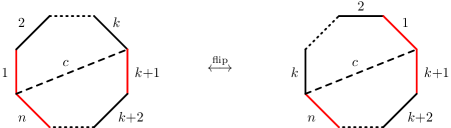
Figure 3: Example of an admissible flip by a chord $c$ between $n$-gons labelled by $(1,\underline{2},\ldots,\underline{k},k{+}1,\underline{k{+}2},\ldots,n)$ and $(\underline{k},\ldots,\underline{2},1,k{+}1,\underline{k{+}2},\ldots,n)$. Edges corresponding to unintegrated punctures are indicated in red. Flipped side of the $n$-gon contains only one red edge, which makes the flip admissible.

A given chord is admissible only if the result of the flip leaves the fixed labels $(1,p{+2},p{+}3,\ldots,n)$ in the same order. In other words, the side of the $n$-gon we flip has to have exactly $0$ or $1$ edges corresponding to fixed punctures. (In particular, for $p=n{-}3$ all chords are admissible.) To every chord $c$ we associate the Mandelstam variable

$$s_{c}=\alpha^{\prime}\left(\sum_{i\in F_{c}}k_{i}\right)^{2},$$ (6.21)

where $F_{c}$ is the set of edges being flipped ($2\leq|F_{c}|\leq n{-}2$). In the example of figure 3 we have $s_{c}=s_{12\ldots k}$. If a chord is admissible, it labels an element of the boundary of $\gamma_{a}^{(n,p)}$, and the whole boundary structure is governed by how these chords fit into tessellations. The cycles $\gamma_{a}^{(n,p)}$ are combinatorially isomorphic to Stasheff polytopes and their direct products.

6.3.1 Self-intersection numbers

A given tessellation $T_{a}$ associated to $\gamma_{a}^{(n,p)}$ is admissible if it includes only admissible chords $\{c_{\ell}\}_{\ell=1,2,\ldots,|T_{a}|}\in T_{a}$, where $|T_{a}|\in\{0,1,\ldots,p\}$ is the number of chords used, and one imposes that these chords do not cross. Following MANA:MANA19941660122 ; doi:10.1002/mana.19941680111 we find the following formula for self-intersection numbers:

$$\langle\gamma_{a}^{(n,p)}|\gamma_{a}^{(n,p)}\rangle=(2i)^{p}\sum_{T_{a}}\prod_{c_{\ell}\in T_{a}}\frac{1}{e^{2\pi is_{c_{\ell}}}-1},$$ (6.22)

where the sum goes over all admissible tessellations (for $|T_{a}|=0$ the set of chords is empty and the term contributing to the sum is $1$) and we introduce the following shorthand

$$t_{ij\ldots}=e^{2\pi is_{ij\ldots}}-1\,.$$ (6.23)

The geometric understanding of this formula is that a given tessellation $T_{a}$ with $|T_{a}|$ chords labels the codimension-$|T_{a}|$ boundary of $\gamma_{a}^{(n,p)}$. For example, the terms with maximum number of chords, $\max|T_{a}|$, label its vertices, and those with a single chord label its facets. Tessellations describe the combinatorics of how these elements of the boundary fit together.

For example, at $p=1$:

$$\langle\gamma_{1\underline{2}3\cdots n}^{(n,1)}|\gamma_{1\underline{2}3\cdots n}^{(n,1)}\rangle=2i\left(1+\frac{1}{t_{12}}+\frac{1}{t_{23}}\right)=\frac{\sin(\pi(s_{12}{+}s_{23}))}{\sin(\pi s_{12})\sin(\pi s_{23})}\,.$$ (6.24)

Here and below, to make the connection with $n$-gons easier to follow, we label the cycles $\gamma_{a}^{(n,p)}$ directly by their permutation $\rho_{a}$ and underline the integrated (unfixed) labels. For $p=2$ the answer depends on the number of fixed punctures separating the two unfixed ones:

$$\langle\gamma_{1\underline{2}\underline{3}4\cdots n}^{(n,2)}|\gamma_{1\underline{2}\underline{3}4\cdots n}^{(n,2)}\rangle=-4\bigg{(} \,1+\frac{1}{t_{12}}+\frac{1}{t_{23}}+\frac{1}{t_{34}}+\frac{1}{t_{123}}+\frac{1}{t_{234}}$$ (6.25)

$$+\frac{1}{t_{12}t_{34}}+\frac{1}{t_{12}t_{123}}+\frac{1}{t_{23}t_{123}}+\frac{1}{t_{23}t_{234}}+\frac{1}{t_{34}t_{234}}\bigg{)}\,,$$

$$\langle\gamma_{1\underline{2}4\underline{3}5\cdots n}^{(n,2)}|\gamma_{1\underline{2}4\underline{3}5\cdots n}^{(n,2)}\rangle=-4\bigg{(} \,1+\frac{1}{t_{12}}+\frac{1}{t_{24}}+\frac{1}{t_{34}}+\frac{1}{t_{35}}+\frac{1}{t_{234}}$$ (6.26)

$$+\frac{1}{t_{12}t_{34}}+\frac{1}{t_{12}t_{35}}+\frac{1}{t_{24}t_{35}}+\frac{1}{t_{24}t_{234}}+\frac{1}{t_{34}t_{234}}\bigg{)}\,,$$

and

$$\langle\gamma_{1\underline{2}4\ldots k\underline{3}k+1\cdots n}^{(n,2)}|\gamma_{1\underline{2}45\underline{3}6\cdots n}^{(n,2)}\rangle=-4\left(1+\frac{1}{t_{12}}+\frac{1}{t_{24}}\right)\left(1+\frac{1}{t_{3k}}+\frac{1}{t_{3,k+1}}\right)$$ (6.27)

for $k\geq 5$. Factorization of the final example reflects the fact that the corresponding chamber is combinatorially a square (a product of two one-dimensional Stasheff polytopes), while the first two were two-dimensional Stasheff polytopes, combinatorially pentagons.

6.3.2 Generic intersection numbers

A more interesting case is the intersection number of distinct cycles, which geometrically describes the boundary of their intersection in the moduli space. If two $n$-gons cannot be transformed into one another with a series of admissible flips, their intersection number is zero. Otherwise, associated to $\gamma_{a}^{(n,p)}$ and $\gamma_{b}^{(n,p)}$, there exists a unique set of chords $T_{ab}$ that flips one into another in the minimal number of steps, as illustrated in figure 4.

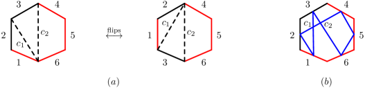
Figure 4: $(a)$ Example of the tessellation $T_{ab}$ by admissible chords $c_{1},c_{2}$ for $\gamma_{1\underline{23}456}^{(6,2)}$ and $\gamma_{\underline{3}1\underline{2}456}^{(6,2)}$. We have $s_{c_{1}}=s_{12}$ and $s_{c_{2}}=s_{123}$. $(b)$ The set of chords can be determined, following Cachazo:2013iea ; Mizera:2016jhj , by embedding the second $n$-gon (blue) inside the first one by connecting midpoints of its edges in the order $\rho_{b}$. Provided this can be done without self-overlaps, the chords are determined by places where the second $n$-gon folds over (admissibility criteria need to be checked separately).

The resulting $n$-gon is tessellated into a number of smaller polygons $P_{ab}$. For each $P_{ab}$ we can define the set of admissible tessellations $T_{P_{ab}}$ that have chords only within $P_{ab}$ (admissibility is determined with respect to the original $n$-gon). The formula for the intersection number becomes

$$\langle\gamma_{a}^{(n,p)}|\gamma_{b}^{(n,p)}\rangle=(-1)^{w(\rho_{a}|\rho_{b})+1}\left(\prod_{c_{\ell}\in T_{ab}}\frac{1}{\sin(\pi s_{c_{\ell}})}\right)\prod_{P_{ab}}(2i)^{\max|T_{P_{ab}}|}\sum_{T_{P_{ab}}}\prod_{c_{\ell}\in T_{P_{ab}}}\frac{1}{e^{2\pi is_{c_{\ell}}}-1}\,,$$ (6.28)

where $w(\rho_{a}|\rho_{b})$ is the relative winding number of the two permutations as defined in (Mizera:2016jhj, , Appendix A). The proof of this formula is analogous to those in MANA:MANA19941660122 ; Mizera:2017cqs . The definition collapses to (6.22) when $a=b$ because $T_{ab}$ is the empty set and $P_{ab}$ is simply the original $n$-gon, so $T_{P_{ab}}=T_{ab}$ and $\max|T_{P_{ab}}|=p$.

For example, let us compute the intersection number of $\gamma_{1\underline{23}456}^{(6,2)}$ and $\gamma_{\underline{3}1\underline{2}456}^{(6,2)}$, which we already know is non-zero from figure 4. We found two chords defining $T_{ab}$, which dissects the original $6$-gon into three polygons we will call $\{P_{1},P_{2},P_{3}\}\ni P_{ab}$ below. For each polygon we find that there is exactly one admissible tessellation, see figure 5.

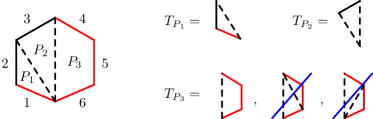
Figure 5: Example polygon decomposition needed for the computation of the intersection number in (6.29). Out of the three polygons, $P_{1}$ and $P_{2}$ are triangles and hence admit only one admissible tessellation. The last one, $P_{3}$, has three possible tessellation, but the last two are not admissible as they separate two red edges on either side of the additional chord.

In this case the winding number is $w(123456|312456)=2$. This leaves us with the final answer:

$$\langle\gamma_{1\underline{23}456}^{(6,2)}|\gamma_{\underline{3}1\underline{2}456}^{(6,2)}\rangle=\frac{(-1)^{2+1}}{\sin(\pi s_{12})\sin(\pi s_{123})}\times 1\times 1\times 1\,.$$ (6.29)

As another example, we can consider the intersection of $\gamma_{1\underline{234}56}^{(6,3)}$ and $\gamma_{\underline{3}1\underline{24}56}^{(6,3)}$, which only differs from (6.29) by the fact that the label $4$ is now integrated. Hence, all the computations are identical, except for the fact that the final two tessellations in $T_{P_{3}}$ of figure 5 are now admissible. We therefore find

$$\langle\gamma_{1\underline{234}56}^{(6,3)}|\gamma_{\underline{3}1\underline{24}56}^{(6,3)}\rangle =\frac{(-1)^{2+1}}{\sin(\pi s_{12})\sin(\pi s_{123})}\times 1\times 1\times 2i\left(1+\frac{1}{t_{45}}+\frac{1}{t_{56}}\right)$$

$$=-\frac{\sin(\pi(s_{45}{+}s_{56}))}{\sin(\pi s_{12})\sin(\pi s_{123})\sin(\pi s_{45})\sin(\pi s_{56})}\,.$$ (6.30)

Another way of stating this result is that the intersection of the two cycles is a one-dimensional Stasheff polytope, while in (6.29) it was a zero-dimensional one (a point).

We will provide more examples in the following subsections. Alternative prescriptions for computing intersection numbers $\langle\gamma_{a}^{(n,p)}|\gamma_{b}^{(n,p)}\rangle$ were given in Mimachi2003 ; mimachi2004 . The advantage of our approach is that it provides combinatorial insight in terms of tessellations of $n$-gons (or equivalently planar trees).

6.4 Case $p=1$

Let us start with an instructive case of $p=1$, which will inspire the choice of bases of cycles for the $p>1$ cases as well. Recall that $d^{(n,1)}=n{-}3$ and the canonical basis of cycles we use is

$$\gamma_{1}^{(n,1)} =\{z_{2}\in\mathbb{R}\,|\,z_{1}<z_{2}<z_{3}<\cdots<z_{n}\}\,,$$ (6.31)

$$\gamma_{a}^{(n,1)} =\{z_{2}\in\mathbb{R}\,|\,z_{1}<\cdots<z_{a+1}<z_{2}<z_{a+2}<\cdots<z_{n}\}\quad\mathrm{for}\quad 2\leq a\leq n{-}3\,,$$

or in the notation introduced above

$$\gamma_{a}^{(n,1)}=\left(\gamma_{1\underline{2}34\ldots n}^{(n,1)},\;\gamma_{13\underline{2}4\ldots n}^{(n,1)},\;\ldots,\;\gamma_{134\ldots n-2,\underline{2},n-1,n}^{(n,1)}\right)_{a}\,.$$ (6.32)

6.4.1 Symmetric bases

Let us compute the intersection matrix $H_{ab}^{(n,1)}$ in (6.17) explicitly. For the $n$-gon associated to $\gamma_{\ldots j\underline{2}k\ldots}^{(n,1)}$, only two chords $c_{s_{j2}},c_{s_{2k}}$ are admissible: precisely those corresponding to the Mandelstam invariants $s_{j2},s_{2k}$. Hence, we conclude that elements in the basis (6.32) which are more than one element apart have no common chords and thereby zero intersection number.

It remains to consider the other two cases. For the self-intersection number, we already computed the answer in (6.24), which after relabeling and expressing in terms of trigonometric functions gives

$$\langle\gamma_{\ldots j\underline{2}k\ldots}^{(n,1)}|\gamma_{\ldots j\underline{2}k\ldots}^{(n,1)}\rangle=\frac{\sin(\pi(s_{j2}{+}s_{2k}))}{\sin(\pi s_{j2})\sin(\pi s_{2k})}=\cot(\pi s_{j2})+\cot(\pi s_{2k})\,.$$ (6.33)

Two adjacent cycles $\gamma_{\ldots j\underline{2}k,k+1,\ldots}^{(n,1)}$ and $\gamma_{\ldots jk\underline{2},k+1,\ldots}^{(n,1)}$ share a single chord $c_{s_{2k}}$, which decomposes the $n$-gon into a triangle $P_{1}$ and an $(n{-}1)$-gon $P_{2}$. Both of these have only one admissible empty tessellation, which is given by the polytope itself, $T_{P_{i}}=P_{i}$. Together with the fact that the relative winding number of the two permutations is $2$, we have

$$\langle\gamma_{\ldots j\underline{2}k,k+1,\ldots}^{(n,1)}|\gamma_{\ldots jk\underline{2},k+1,\ldots}^{(n,1)}\rangle=-\frac{1}{\sin(\pi s_{2k})}=-\csc(\pi s_{2k})$$ (6.34)

and the same result for $\langle\gamma_{\ldots jk\underline{2},k+1,\ldots}^{(n,1)}|\gamma_{\ldots j\underline{2}k,k+1,\ldots}^{(n,1)}\rangle$ by hermitian symmetry of the intersection product. Organizing these results into an $(n{-}3)\times(n{-}3)$ symmetric tridiagonal matrix we obtain

$$H^{(n,1)}=\left(\begin{array}[]{cccc}\cot(\pi s_{12}){+}\cot(\pi s_{23})&-\csc(\pi s_{23})&0&\cdots\\ -\csc(\pi s_{23})&\cot(\pi s_{23}){+}\cot(\pi s_{24})&-\csc(\pi s_{24})&\cdots\\ 0&-\csc(\pi s_{24})&\cot(\pi s_{24}){+}\cot(\pi s_{25})&\cdots\\ \vdots&\vdots&\vdots&\ddots\end{array}\right)\,.$$ (6.35)

We find that these matrices have the inverse with entries (recall that $s_{ii}=0$):

$$(H^{(n,1)})^{-1}_{ab}=\frac{\sin(\pi\sum_{i=1}^{\min(a,b)+1}s_{2i})\sin(\pi\sum_{i=\max(a,b)+2}^{n-1}s_{2i})}{\sin(\pi\sum_{i=1}^{n-1}s_{2i})}\,.$$ (6.36)

6.4.2 Alternative bases

In spite of the appeal of a symmetric basis choice for the entries of $\tilde{H}^{(n,p)}_{ab}$, we found a more convenient choice of bases that simplifies the entries of the KLT matrix. Let us denote the corresponding intersection matrix by

$$\tilde{H}^{(n,1)}_{ab}=\langle\gamma_{a}^{(n,1)}|\tilde{\gamma}_{b}^{(n,1)}\rangle\,,$$ (6.37)

where the right basis is now taken to be

$$\tilde{\gamma}_{a}^{(n,1)}=\left(\gamma_{\underline{2}134\ldots n}^{(n,1)},\;\gamma_{1\underline{2}34\ldots n}^{(n,1)},\;\ldots,\;\gamma_{134\ldots n-3,\underline{2},n-2,n-1,n}^{(n,1)}\right)_{a}\,.$$ (6.38)

We simply “shifted” the position of $2$ by one slot to the left compared to (6.32) which effectively moves the diagonals of the intersection matrix and leads to the new form

$$\tilde{H}^{(n,1)}=\left(\begin{array}[]{cccc}-\csc(\pi s_{12})&\cot(\pi s_{12}){+}\cot(\pi s_{23})&-\csc(\pi s_{23})&\cdots\\ 0&-\csc(\pi s_{23})&\cot(\pi s_{23}){+}\cot(\pi s_{24})&\cdots\\ 0&0&-\csc(\pi s_{24})&\cdots\\ \vdots&\vdots&\vdots&\ddots\end{array}\right)\,.$$ (6.39)

This fact is crucial in simplifying the computation of the inverse, which can easily be seen to take the upper-triangular form

$$(\tilde{H}^{(n,1)})^{-1}=-\left(\begin{array}[]{cccc}\sin(\pi s_{12})&\sin(\pi(s_{12}{+}s_{23}))&\sin(\pi(s_{12}{+}s_{23}{+}s_{24}))&\cdots\\ 0&\sin(\pi s_{23})&\sin(\pi(s_{23}{+}s_{24}))&\cdots\\ 0&0&\sin(\pi s_{24})&\cdots\\ \vdots&\vdots&\vdots&\ddots\end{array}\right)\,,$$ (6.40)

or more explicitly

$$(\tilde{H}^{(n,1)})_{ab}^{-1}=-\sin\bigg{(}\pi\sum_{i=a+1-\delta_{a1}}^{b+1}s_{2i}\bigg{)}\,.$$ (6.41)

The entries vanish for $b<a$ and are polynomial in terms of the sines, i.e. do not have any analogue of the denominator in (6.36). This choice of bases will inform the choices for general $(n,p)$.

The matrix entries in (6.41) can be used to compute $\beta_{a}^{(n,1)}$ cycles in terms of the basis $\tilde{\gamma}_{a}^{(n,1)}$ needed in the definition of the integrals $I_{ab}^{(n,1)}$ given in (6.14). Using (6.15) and (6.20) we have, for instance,

$$\beta^{(4,1)}_{1}=-\sin(\pi s_{12})\gamma_{\underline{2}134}^{(4,1)}\,,$$ (6.42)

as well as

$$\beta^{(5,1)}_{1} =-\sin(\pi s_{12})\gamma_{\underline{2}1345}^{(5,1)}\,,$$

$$\beta^{(5,1)}_{2} =-\sin(\pi(s_{12}{+}s_{23}))\gamma_{\underline{2}1345}^{(5,1)}-\sin(\pi s_{23})\gamma_{1\underline{2}345}^{(5,1)}\,,$$ (6.43)

and

$$\beta^{(6,1)}_{1} =-\sin(\pi s_{12})\gamma_{\underline{2}13456}^{(6,1)}\,,$$

$$\beta^{(6,1)}_{2} =-\sin(\pi(s_{12}{+}s_{23}))\gamma_{\underline{2}13456}^{(6,1)}-\sin(\pi s_{23})\gamma_{1\underline{2}3456}^{(6,1)}\,,$$ (6.44)

$$\beta^{(6,1)}_{3} =-\sin(\pi(s_{12}{+}s_{23}{+}s_{24}))\gamma_{\underline{2}13456}^{(6,1)}-\sin(\pi(s_{23}{+}s_{24}))\gamma_{1\underline{2}3456}^{(6,1)}-\sin(\pi s_{24})\gamma_{13\underline{2}456}^{(6,1)}\,.$$

6.4.3 Overcomplete form of KLT relations

Before looking at $p=2$ examples, let us see how the same results could have been obtained from the overcomplete (but extremely simple) form of the KLT relations from (6.12). We can write them with an $(n{-}1)\times(n{-}1)$ kernel matrix $\Phi$ with entries $\Phi_{ab}=\tfrac{i}{2}e^{i\pi\phi_{ab}}$ given by (6.13). More explicitly, we have

$$\Phi=\frac{i}{2}\left(\begin{array}[]{ccccc}1&e^{i\pi s_{12}}&e^{i\pi(s_{12}+s_{23})}&\cdots&e^{i\pi\sum_{i=1}^{n-1}s_{2i}}\\ e^{i\pi s_{12}}&1&e^{i\pi s_{23}}&\cdots&e^{i\pi\sum_{i=3}^{n-1}s_{2i}}\\ e^{i\pi(s_{12}+s_{23})}&e^{i\pi s_{23}}&1&\cdots&e^{i\pi\sum_{i=4}^{n-1}s_{2i}}\\ \vdots&\vdots&\vdots&\ddots&\vdots\\ e^{i\pi\sum_{i=1}^{n-1}s_{2i}}&e^{i\pi\sum_{i=3}^{n-1}s_{2i}}&e^{i\pi\sum_{i=4}^{n-1}s_{2i}}&\cdots&1\end{array}\right),$$ (6.45)

where the columns and rows are labelled by all cycles in $\mathbb{R}\setminus\{z_{2}=z_{j}\}$,

$$\Gamma=\left(\gamma_{\underline{2}134\ldots n}^{(n,1)},\;\gamma_{1\underline{2}34\ldots n}^{(n,1)},\;\ldots,\;\gamma_{134\ldots n-1,\underline{2},n}^{(n,1)}\right)^{t}.$$ (6.46)

In order to reduce this to the $(n{-}3)\times(n{-}3)$ form, one makes use of the fact that only $n{-}3$ cycles in (6.46) are linearly dependent. They satisfy a pair of monodromy relations Plahte:1970wy ; BjerrumBohr:2009rd ; Stieberger:2009hq :

$$\left(\begin{array}[]{ccccc}1&e^{i\pi s_{12}}&e^{i\pi(s_{12}+s_{23})}&\cdots&e^{i\pi\sum_{i=1}^{n-1}s_{2i}}\\ 1&e^{-i\pi s_{12}}&e^{-i\pi(s_{12}+s_{23})}&\cdots&e^{-i\pi\sum_{i=1}^{n-1}s_{2i}}\end{array}\right)\Gamma=\begin{pmatrix}0\\ 0\end{pmatrix},$$ (6.47)

where $s_{22}=0$ and the first (second) row comes from considering a contour right above (below) the real $z_{2}$-axis and deforming it to a point in the upper-half (lower-half) plane, also see appendix A.1. Let us invert these relations to construct projectors onto the two bases (6.32), (6.38) we considered in this subsection. We can write $(\Gamma_{1},\Gamma_{n-1})P=\Gamma$ with

$$P =-\left(\begin{array}[]{cc}1&e^{i\pi\sum_{i=1}^{n-1}s_{2i}}\\ 1&e^{-i\pi\sum_{i=1}^{n-1}s_{2i}}\end{array}\right)^{-1}\left(\begin{array}[]{cccc}e^{i\pi s_{12}}&e^{i\pi(s_{12}+s_{23})}&\cdots&e^{i\pi\sum_{i=1}^{n-2}s_{2i}}\\ e^{-i\pi s_{12}}&e^{-i\pi(s_{12}+s_{23})}&\cdots&e^{-i\pi\sum_{i=1}^{n-2}s_{2i}}\end{array}\right)$$ (6.52)

$$=\frac{1}{\sin(\pi s_{2n})}\left(\begin{array}[]{cccc}\sin(\pi\sum_{i=3}^{n-1}s_{2i})&\sin(\pi\sum_{i=4}^{n-1}s_{2i})&\cdots&\sin(\pi s_{2,n-1})\\ \sin(\pi s_{12})&\sin(\pi(s_{12}{+}s_{23}))&\cdots&\sin(\pi\sum_{i=1}^{n-2}s_{2i})\end{array}\right),$$ (6.55)

which expresses the first and last elements of $\Gamma$ in terms of the basis $\gamma^{(n,1)}_{a}$. Similarly, eliminating the second-last and last elements we have a projector onto the $\tilde{\gamma}^{(n,1)}_{a}$ basis:

$$\tilde{P} =-\left(\begin{array}[]{cc}e^{i\pi\sum_{i=1}^{n-2}s_{2i}}&e^{i\pi\sum_{i=1}^{n-1}s_{2i}}\\ e^{-i\pi\sum_{i=1}^{n-2}s_{2i}}&e^{-i\pi\sum_{i=1}^{n-1}s_{2i}}\end{array}\right)^{-1}\left(\begin{array}[]{ccccc}1&e^{i\pi s_{12}}&e^{i\pi(s_{12}+s_{23})}&\cdots&e^{i\pi\sum_{i=1}^{n-3}s_{2i}}\\ 1&e^{-i\pi s_{12}}&e^{-i\pi(s_{12}+s_{23})}&\cdots&e^{-i\pi\sum_{i=1}^{n-3}s_{2i}}\end{array}\right)$$ (6.60)

$$=\frac{1}{\sin(\pi s_{2,n-1})}\left(\begin{array}[]{cccc}{-}\sin(\pi\sum_{i=1}^{n-1}s_{2i})&{-}\sin(\pi\sum_{i=3}^{n-1}s_{2i})&\cdots&{-}\sin(\pi(s_{2,n-2}{+}s_{2,n-1}))\\ \sin(\pi\sum_{i=1}^{n-2}s_{2i})&\sin(\pi\sum_{i=3}^{n-2}s_{2i})&\cdots&\sin(\pi s_{2,n-2})\end{array}\right)\,.$$ (6.63)

With these computations in place, we can simply apply the projectors to the relevant columns and rows of the overcomplete KLT matrix to obtain:

$$\begin{pmatrix}P_{1}\\ \mathds{1}_{n-3}\\ P_{2}\end{pmatrix}^{\!\!t}\Phi\begin{pmatrix}P_{1}\\ \mathds{1}_{n-3}\\ P_{2}\end{pmatrix}=(H^{(n,1)})^{-1}\,,\qquad\begin{pmatrix}\mathds{1}_{n-3}\\ \tilde{P}_{1}\\ \tilde{P}_{2}\end{pmatrix}^{\!\!t}\Phi\begin{pmatrix}P_{1}\\ \mathds{1}_{n-3}\\ P_{2}\end{pmatrix}=(\tilde{H}^{(n,1)})^{-1}\,,$$ (6.64)

reproducing the results from (6.36) and (6.41).

6.5 Case $p=2$

Recall that for $p=2$ the basis $\gamma_{a}^{(n,2)}$ consists of all cycles where $z_{1}<z_{4}<z_{5}<\cdots<z_{n}=\infty$ are fixed in this order and $z_{2},z_{3}$ are placed between $z_{1}=0$ and $z_{n-1}=1$, for the total of $d^{(n,2)}=(n{-}3)(n{-}4)$ elements in the basis.

Motivated by the simplicity of the results for $p=1$, we will also introduce a second basis $\tilde{\gamma}_{a}^{(n,2)}$ where $z_{2},z_{3}$ are placed between $z_{n}=-\infty$ and $z_{n-2}$ (or $z_{1}$ for $p=n{-}3$). To make the notation a bit more clear and recognize a pattern, let us compute the KLT kernel for the examples $n=5,6$.

6.5.1 Example $(n,p)=(5,2)$

The two bases are given by

$$\gamma_{a}^{(5,2)}=\left(\gamma_{1\underline{23}45}^{(5,2)},\;\gamma_{1\underline{32}45}^{(5,2)}\right)_{a},\qquad\tilde{\gamma}_{b}^{(5,2)}=\left(\gamma_{\underline{23}145}^{(5,2)},\;\gamma_{\underline{32}145}^{(5,2)}\right)_{b}.$$ (6.65)

Computing the intersection matrix according to the above combinatorial rules we find

$$\tilde{H}^{(5,2)}=\csc(\pi s_{123})\left(\begin{array}[]{cc}-\csc(\pi s_{23})&\cot(\pi s_{12})+\cot(\pi s_{23})\\ \cot(\pi s_{13})+\cot(\pi s_{23})&-\csc(\pi s_{23})\end{array}\right)\,,$$ (6.66)

where the tilde refers to the asymmetric basis choice $\tilde{H}^{(5,2)}_{ab}=\langle\gamma_{a}^{(5,2)}|\tilde{\gamma}_{b}^{(5,2)}\rangle$ analogous to (6.37). Inverting the matrix we obtain the well-known result for the local KLT matrix

$$(\tilde{H}^{(5,2)})^{-1}=\left(\begin{array}[]{cc}\sin(\pi s_{12})\sin(\pi s_{13})&\sin(\pi s_{13})\sin(\pi(s_{12}{+}s_{23}))\\ \sin(\pi s_{12})\sin(\pi(s_{13}{+}s_{23}))&\sin(\pi s_{12})\sin(\pi s_{13})\end{array}\right)\,,$$ (6.67)

in agreement with momentum-kernel techniques momentumKernel . With this result the basis cycles $\beta_{a}^{(5,2)}$ in (6.14) and (6.16) read as follows,

$$\beta_{1}^{(5,2)}=\sin(\pi s_{12})\left(\sin(\pi s_{13})\gamma_{\underline{23}145}^{(5,2)}+\sin(\pi(s_{13}{+}s_{23}))\gamma_{\underline{32}145}^{(5,2)}\right)\,,$$

$$\beta_{2}^{(5,2)}=\sin(\pi s_{13})\left(\sin(\pi(s_{12}{+}s_{23}))\gamma_{\underline{23}145}^{(5,2)}+\sin(\pi s_{12})\gamma_{\underline{32}145}^{(5,2)}\right)\,.$$ (6.68)

6.5.2 Example $(n,p)=(6,2)$

In this case the two bases are given by

$$\gamma_{a}^{(6,2)}=\left(\gamma_{1\underline{23}456}^{(6,2)},\;\gamma_{1\underline{2}4\underline{3}56}^{(6,2)},\;\gamma_{1\underline{32}456}^{(6,2)},\;\gamma_{1\underline{3}4\underline{2}56}^{(6,2)},\;\gamma_{14\underline{23}56}^{(6,2)},\;\gamma_{14\underline{32}56}^{(6,2)}\right)_{a},$$ (6.69)

$$\tilde{\gamma}_{b}^{(6,2)}=\left(\gamma_{\underline{23}1456}^{(6,2)},\;\gamma_{\underline{2}1\underline{3}456}^{(6,2)},\;\gamma_{1\underline{23}456}^{(6,2)},\;\gamma_{\underline{32}1456}^{(6,2)},\;\gamma_{\underline{3}1\underline{2}456}^{(6,2)},\;\gamma_{1\underline{32}456}^{(6,2)}\right)_{b}\,.$$ (6.70)

Among the intersection numbers $\tilde{H}^{(6,2)}_{ab}=\langle\gamma_{a}^{(6,2)}|\tilde{\gamma}_{b}^{(6,2)}\rangle$ in the asymmetric basis choice, we already computed one example in the entry $\tilde{H}_{15}^{(6,2)}$ in (6.29). Due to space limitations we do not present the full intersection matrix here. Its $6\times 6$ inverse, however, takes a relatively compact form:

$$(\tilde{H}^{(6,2)})^{-1}=\left(\begin{array}[]{ccc}\sin(\pi s_{12})\sin(\pi s_{13})&\sin(\pi s_{12})\sin(\pi s_{14,3})&\sin(\pi s_{13})\sin(\pi s_{13,2})\\ 0&\sin(\pi s_{12})\sin(\pi s_{34})&0\\ 0&0&0\\ \sin(\pi s_{12})\sin(\pi s_{12,3})&\sin(\pi s_{12})\sin(\pi s_{124,3})&\sin(\pi s_{12})\sin(\pi s_{13})\\ 0&0&0\\ 0&0&0\\ \end{array}\right.$$ (6.71)

$$\qquad\qquad\left.\begin{array}[]{ccc}\sin(\pi s_{13})\sin(\pi s_{134,2})&\sin(\pi s_{14,2})\sin(\pi s_{14,3})&\sin(\pi s_{14,3})\sin(\pi s_{134,2})\\ 0&\sin(\pi s_{34})\sin(\pi s_{14,2})&\sin(\pi s_{34})\sin(\pi s_{134,2})\\ 0&\sin(\pi s_{24})\sin(\pi s_{34})&\sin(\pi s_{34})\sin(\pi s_{34,2})\\ \sin(\pi s_{13})\sin(\pi s_{14,2})&\sin(\pi s_{14,2})\sin(\pi s_{124,3})&\sin(\pi s_{14,2})\sin(\pi s_{14,3})\\ \sin(\pi s_{13})\sin(\pi s_{24})&\sin(\pi s_{24})\sin(\pi s_{124,3})&\sin(\pi s_{24})\sin(\pi s_{14,3})\\ 0&\sin(\pi s_{24})\sin(\pi s_{24,3})&\sin(\pi s_{24})\sin(\pi s_{34})\\ \end{array}\right)\,,$$

where we use the notation $s_{i_{1}i_{2}\ldots,j}=s_{i_{1}j}+s_{i_{2}j}+\cdots$. In terms of the $\beta_{a}^{(6,2)}$ cycles from (6.14), this translates to

$$\beta_{1}^{(6,2)} =\sin(\pi s_{12})\left(\sin(\pi s_{13})\gamma^{(6,2)}_{\underline{23}1456}+\sin(\pi s_{12,3})\gamma^{(6,2)}_{\underline{32}1456}\right)\,,$$

$$\beta_{2}^{(6,2)} =\sin(\pi s_{12})\left(\sin(\pi s_{14,3})\gamma^{(6,2)}_{\underline{23}1456}+\sin(\pi s_{34})\gamma^{(6,2)}_{\underline{2}1\underline{3}456}+\sin(\pi s_{124,3})\gamma^{(6,2)}_{\underline{32}1456}\right)\,,$$

$$\beta_{3}^{(6,2)} =\sin(\pi s_{13})\left(\sin(\pi s_{13,2})\gamma^{(6,2)}_{\underline{23}1456}+\sin(\pi s_{12})\gamma^{(6,2)}_{\underline{32}1456}\right)\,,$$ (6.72)

$$\beta_{4}^{(6,2)} =\sin(\pi s_{13})\left(\sin(\pi s_{134,2})\gamma^{(6,2)}_{\underline{23}1456}+\sin(\pi s_{14,2})\gamma^{(6,2)}_{\underline{32}1456}+\sin(\pi s_{24})\gamma^{(6,2)}_{\underline{3}1\underline{2}456}\right)\,,$$

$$\beta_{5}^{(6,2)} =\sin(\pi s_{14,2})\left(\sin(\pi s_{14,3})\gamma_{\underline{23}1456}^{(6,2)}+\sin(\pi s_{34})\gamma_{\underline{2}1\underline{3}456}^{(6,2)}+\sin(\pi s_{124,3})\gamma_{\underline{32}1456}^{(6,2)}\right)$$

$$\quad+\sin(\pi s_{24})\left(\sin(\pi s_{34})\gamma_{1\underline{23}456}^{(6,2)}+\sin(\pi s_{124,3})\gamma_{\underline{3}1\underline{2}456}^{(6,2)}+\sin(\pi s_{24,3})\gamma_{1\underline{32}456}^{(6,2)}\right)\,,$$

$$\beta_{6}^{(6,2)} =\sin(\pi s_{34})\left(\sin(\pi s_{134,2})\gamma_{\underline{2}1\underline{3}456}^{(6,2)}+\sin(\pi s_{34,2})\gamma_{1\underline{23}456}^{(6,2)}+\sin(\pi s_{24})\gamma_{1\underline{32}456}^{(6,2)}\right)$$

$$\quad+\sin(\pi s_{14,3})\left(\sin(\pi s_{134,2})\gamma_{\underline{23}1456}^{(6,2)}+\sin(\pi s_{14,2})\gamma_{\underline{32}1456}^{(6,2)}+\sin(\pi s_{24})\gamma_{\underline{3}1\underline{2}456}^{(6,2)}\right)\,.$$

This example already illustrates the general rule: For each integrated puncture $i\in\{2,3\}$ we have a sine factor in the generalized KLT kernel $S_{\alpha^{\prime}}$ in (6.20). The arguments of the sine functions are given by the overlap between labels to the left of $i$ in $\gamma_{a}^{(6,2)}$ which are also to the right of $i$ in $\tilde{\gamma}_{b}^{(6,2)}$. We make this observation more concrete in the following.

6.6 Recursion for general $(n,p)$

The goal of this subsection is to find the explicit form of the cycles $\beta^{(n,p)}$ in (6.14) which need to be field-theory orthonormal with respect to the forms $\nu^{(n,p)}$ that are the Betti–de Rham duals of the integration cycles

$$\gamma^{(n,p)}_{\vec{A},\vec{i}}\quad\leftrightarrow\quad\rho_{\vec{A},\vec{i}}=(1,A_{1},\underline{i_{1}},A_{2},\underline{i_{2}},\ldots,A_{p},\underline{i_{p}},A_{p+1},n{-}1,n)$$ (6.73)

in order to avoid inconsistency in the $\alpha^{\prime}\rightarrow 0$ limit of (6.16).

As in section 2.3, we gather the unintegrated punctures different from $(z_{1},z_{n-1},z_{n})=(0,1,\infty)$ in a vector $\vec{A}$ of words $A_{1},A_{2},\ldots$ each of which gathers (possibly zero) adjacent unintegrated punctures. The $i_{1},i_{2},\ldots,i_{p}$ in turn are a permutation of the $p$ integrated punctures $z_{2},z_{3},\ldots,z_{p+1}$.

The examples of the $\beta^{(n,p)}$ in the earlier subsections have orthonormal intersection numbers with the $\gamma^{(n,p)}$ in (6.73) in the sense that

$$\langle\gamma^{(n,p)}_{\vec{A},\vec{i}}|\beta^{(n,p)}_{\vec{B},\vec{j}}\rangle=\delta_{\vec{A},\vec{B}}\delta_{\vec{i},\vec{j}}\,.$$ (6.74)

At general $n$ and $p$, the $\beta^{(n,p)}$ with this property are conjecturally given by

$$\beta^{(n,p)}_{\vec{A},\vec{i}}=\sum_{\vec{B},\vec{j}}S_{\alpha^{\prime}}(1,\vec{A},\vec{i}\ |\vec{B},\vec{j},n{-}2)\,\tilde{\gamma}^{(n,p)}_{\vec{B},\vec{j}}\,,$$ (6.75)

where we employ the alternative basis (6.19) of $d^{(n,p)}$ cycles $\tilde{\gamma}^{(n,p)}_{\vec{B},\vec{j}}$ instead of (6.73), in order to obtain a local expression for the generalized KLT kernel $S_{\alpha^{\prime}}$. Since the final two labels are always the same, we suppress them in (6.75) and below for clarity, i.e., $S_{\alpha^{\prime}}(X|Y)=S_{\alpha^{\prime}}(X,n{-}1,n|Y,n{-}1,n)$. The latter is claimed to obey the following recursion in the number of integrated punctures $i_{k}$

$$S_{\alpha^{\prime}}(1,A_{1},\underline{i_{1}},A_{2},\ldots,A_{p},\underline{i_{p}},A_{p+1}|X,\underline{i_{p}},Y)$$ (6.76)

$$=-\sin(2\pi\alpha^{\prime}k_{i_{p}}{\cdot}\textstyle\sum_{\ell\in Y\cap(1,A_{1},i_{1},\ldots,i_{p-1},A_{p})}k_{\ell})\,S_{\alpha^{\prime}}(1,A_{1},\underline{i_{1}},A_{2},\ldots,\underline{i_{p-1}},A_{p},A_{p+1}|X,Y)\,.$$

This step may only be applied to remove the rightmost integrated puncture $i_{p}$ in the first entry, and the recursion terminates with

$$S_{\alpha^{\prime}}(1,\vec{A}\ |\vec{B},n{-}2)=\delta_{(1,\vec{A}),(\vec{B},n{-}2)}$$ (6.77)

when there are no more integrated punctures left. This has been verified up to and including $n=8$ for any value of $p\leq n{-}4$ by checking that $S_{\alpha^{\prime}}$ is indeed the inverse of $\tilde{H}^{(n,p)}$ obtained with combinatorial rules of the previous subsections. More generally, the recursion (6.76) can be rewritten as

$$S_{\alpha^{\prime}}(P,\underline{i},Q|X,\underline{i},Y)=-\sin(2\pi\alpha^{\prime}k_{i}\cdot k_{P\cap Y})\,S_{\alpha^{\prime}}(P,Q|X,Y)\,,$$ (6.78)

where $Q$ has no integrated punctures, i.e., the momenta in the sine functions are determined by the punctures that appear on opposite sides of $i$ in the two entries of $S_{\alpha^{\prime}}(\cdot|\cdot)$. The structure of the recursion (6.78) resonates with the momentum-kernel formalism momentumKernel and its generalization to the KLT formulae for $p=n{-}4$ Vanhove:2018elu .

With the expansion (6.75), the desired orthonormality property (6.74) takes the form (with collective indices $a,b,c$ taking the role of $\vec{A},\vec{i}$),

$$\langle\gamma^{(n,p)}_{a}|\beta_{b}^{(n,p)}\rangle=\sum_{c=1}^{d^{(n,p)}}\langle\gamma_{a}^{(n,p)}|\tilde{\gamma}^{(n,p)}_{c}\rangle(S_{\alpha^{\prime}})_{bc}=\delta_{ab}\,,$$ (6.79)

In order to deduce the desired orthonormality of $\beta_{a}^{(n,p)}$ and $\nu_{b}^{(n,p)}$ in the $\alpha^{\prime}\rightarrow 0$ limit, we insert complete sets of cycles $\gamma^{(n,p)}_{c}$ and cocycles $\overline{\omega_{d}^{(n,p)}}$,

$$\lim_{\alpha^{\prime}\rightarrow 0}\langle\beta_{a}^{(n,p)}|\nu^{(n,p)}_{b}\rangle =\lim_{\alpha^{\prime}\rightarrow 0}\sum_{c,d=1}^{d^{(n,p)}}\langle\beta_{a}^{(n,p)}|\gamma_{c}^{(n,p)}\rangle\,(\overline{F^{(n,p)}})^{-1}_{cd}\,\langle\overline{\omega_{d}^{(n,p)}}|\nu^{(n,p)}_{b}\rangle$$

$$=\sum_{c,d=1}^{d^{(n,p)}}\delta_{ac}\delta_{cd}\delta_{db}=\delta_{ab}\,,$$ (6.80)

where $\overline{F^{(n,p)}_{cd}}=\langle\overline{\omega_{d}^{(n,p)}}|\gamma_{c}^{(n,p)}\rangle=\overline{\langle\gamma_{c}^{(n,p)}|\omega_{d}^{(n,p)}\rangle}$ as in (2.7). The final two Kronecker deltas in passing to the last line stem from the fact that the $\overline{\omega_{d}^{(n,p)}}$ are engineered to be field-theory orthonormal to both $\gamma_{c}^{(n,p)}$ and $\nu^{(n,p)}_{b}$. The first Kronecker delta arises from the conjectural orthonormality (6.79). It would be interesting to find a rigorous all-multiplicity proof that (6.75) together with the recursion (6.76) indeed leads to orthonormal intersection numbers.

7 Implications for minimal models

In this section we give an interpretation of our results in terms of correlation functions in two-dimensional conformal field theories (CFTs). We will focus on the family of theories known as the minimal models whose spectrum can been completely classified and solved in terms of irreducible representations of the Virasoro algebra. We start with a lightning review of these models, where we focus only on the parts necessary to make connections with the rest of this paper. For more comprehensive expositions we refer the reader to dotsenko1988 ; DiFrancesco:1997nk ; Kapec:2020xaj .

7.1 Lightning review of the Coulomb gas formalism

Our starting point is the action of a free boson $\phi(x)$ coupled linearly to the scalar curvature $R$ of the genus-zero surface:

$$S_{\mathfrak{p},\mathfrak{p}^{\prime}}=\int_{\mathbb{CP}^{1}}\mathrm{d}^{2}x\sqrt{g}\left(\frac{1}{2}\partial_{\mu}\phi\partial^{\mu}\phi+\frac{i}{\sqrt{2}}Q_{\mathfrak{p},\mathfrak{p}^{\prime}}\phi R\right).$$ (7.1)

Here the strength of the coupling is given by the background charge $Q_{\mathfrak{p},\mathfrak{p}^{\prime}}$, which makes the $\mathrm{U}(1)$ symmetry anomalous. Since the action is complex, it does not automatically give rise to a unitary theory. In fact, families of unitary models written in this way are heavily constrained and can be classified by a pair of co-prime integers $(\mathfrak{p},\mathfrak{p}^{\prime})$, in terms of which

$$Q_{\mathfrak{p},\mathfrak{p}^{\prime}}=\frac{\mathfrak{p}-\mathfrak{p}^{\prime}}{\sqrt{\mathfrak{p}\mathfrak{p}^{\prime}}}\,.$$ (7.2)

The central charge is $c_{\mathfrak{p},\mathfrak{p}^{\prime}}=1-6Q_{\mathfrak{p},\mathfrak{p}^{\prime}}^{2}$, and we take $\mathfrak{p}>\mathfrak{p}^{\prime}$ by convention. These are the minimal models. For example $(\mathfrak{p},\mathfrak{p}^{\prime})=(4,3)$ gives the critical Ising model with $Q_{4,3}=\frac{1}{2\sqrt{3}}$ and $c_{4,3}=\frac{1}{2}$, while $(\mathfrak{p},\mathfrak{p}^{\prime})=(5,2)$ is the Yang–Lee edge singularity with $Q_{5,2}=\frac{3}{\sqrt{10}}$ and $c_{5,2}=-\frac{22}{5}$.

Conformal primary operators ${\cal O}_{q_{(r,s)}}$ in the $(\mathfrak{p},\mathfrak{p}^{\prime})$ minimal model are classified by two integers $(r,s)$ such that

$$1\leq r\leq\mathfrak{p}^{\prime}{-}1,\qquad 1\leq s\leq\mathfrak{p}{-}1\,.$$ (7.3)

Charges $q_{(r,s)}$ and conformal dimensions $h_{(r,s)}$ of these operators are given by

$$q_{(r,s)}=\frac{\mathfrak{p}(1{-}r)-\mathfrak{p}^{\prime}(1{-}s)}{2\sqrt{\mathfrak{p}\mathfrak{p}^{\prime}}}\,,\qquad h_{(r,s)}=\frac{(r\mathfrak{p}{-}s\mathfrak{p}^{\prime})^{2}-(\mathfrak{p}{-}\mathfrak{p}^{\prime})^{2}}{4\mathfrak{p}\mathfrak{p}^{\prime}}\,.$$ (7.4)

Notice that operators ${\cal O}_{q}$ and ${\cal O}_{Q_{\mathfrak{p},\mathfrak{p}^{\prime}}-q}$ share the same conformal dimension and they are indistinguishable at the level of correlation functions. In other words, we can identify operators with $(r,s)$ and $(\mathfrak{p}^{\prime}{-}r,\mathfrak{p}{-}s)$. For instance, in the case of the critical Ising model with $(\mathfrak{p},\mathfrak{p}^{\prime})=(4,3)$ we have the following Kac table:

$$\begin{array}[]{c||c|c|c}&\medmath{s=1}&\medmath{s=2}&\medmath{s=3}\\ \hline\cr\medmath{r=1}&{\cal O}_{0}=\mathds{1}&{\cal O}_{\frac{\sqrt{3}}{4}}=\sigma&{\cal O}_{\frac{\sqrt{3}}{2}}=\varepsilon\\ \medmath{r=2}&{\cal O}_{-\frac{1}{\sqrt{3}}}=\varepsilon&{\cal O}_{-\frac{1}{4\sqrt{3}}}=\sigma&{\cal O}_{\frac{1}{2\sqrt{3}}}=\mathds{1}\\ \end{array}$$ (7.5)

Here $\mathds{1}$, $\sigma$, and $\varepsilon$ are the usual identity, spin, and energy operators of conformal weight $0$, $\frac{1}{16}$ and $\frac{1}{2}$, respectively.

We will be interested in computing the correlation function of $\mathrm{N}$ such operators. For readability we will simply label the $j$-th vertex operator ${\cal O}_{q_{j}}(x_{j})=e^{i\sqrt{2}q_{j}\phi(x_{j})}$ by its charge $q_{j}$:

$$\langle{\cal O}_{q_{1}}(x_{1}){\cal O}_{q_{2}}(x_{2})\cdots{\cal O}_{q_{\mathrm{N}}}(x_{\mathrm{N}})\rangle_{\mathfrak{p},\mathfrak{p}^{\prime}}\,.$$ (7.6)

Such a computation might not seem approachable, because we deal with a strongly-interacting system. However, one can simplify this problem conceptually using the Coulomb gas formalism Dotsenko:1984nm ; Dotsenko:1984ad , which is the idea that correlation functions in interacting theories with background charge can be equivalently represented as those in a free theory with insertions of $p$ charged operators integrated over the whole surface. As a result, the correlation functions (7.6) can be represented as

$$\int_{(\mathbb{CP}^{1})^{p}}\prod_{i=2}^{p+1}\mathrm{d}^{2}z_{i}\,\langle{\cal O}_{q_{1}}(x_{1}){\cal O}_{q_{2}}(x_{2})\cdots{\cal O}_{q_{\mathrm{N}}}(x_{\mathrm{N}})\prod_{i=2}^{p+1}{\cal O}_{q_{\pm}}(z_{i})\rangle_{\mathrm{free}}$$ (7.7)

up to a constant. The additional operators are called screening charges, and their charges can only take two values, $q_{+}$ and $q_{-}$, given by

$$q_{+}=\sqrt{\mathfrak{p}/\mathfrak{p}^{\prime}}\,,\qquad q_{-}=-\sqrt{\mathfrak{p}^{\prime}/\mathfrak{p}}\,,$$ (7.8)

such that $q_{+}+q_{-}=Q_{\mathfrak{p},\mathfrak{p}^{\prime}}$. We will denote the number of screening charges ${\cal O}_{q_{\pm}}$ by $p_{\pm}$, such that $p_{+}+p_{-}=p$. These numbers can be determined by imposing the neutrality condition (Ward identity), i.e. requiring that the sum of charges equals to the background charge,

$$\sum_{i=1}^{\mathrm{N}}q_{i}\,+\,p_{+}q_{+}\,+\,p_{-}q_{-}\,=\,Q_{\mathfrak{p},\mathfrak{p}^{\prime}}\,.$$ (7.9)

As a heuristic, for sufficiently generic $(\mathfrak{p},\mathfrak{p}^{\prime})$, reading off the coefficients of the irrational numbers $\sqrt{\mathfrak{p}/\mathfrak{p}^{\prime}}$ and $\sqrt{\mathfrak{p}^{\prime}/\mathfrak{p}}$ translates to the following condition for the integers $(r_{i},s_{i})$ labeling every operator:

$$p_{+}=\frac{1}{2}\left(\sum_{i=1}^{\mathrm{N}}r_{i}-\mathrm{N}+2\right)\,,\qquad p_{-}=\frac{1}{2}\left(\sum_{i=1}^{\mathrm{N}}s_{i}-\mathrm{N}+2\right)\,.$$ (7.10)

For instance, the four-point correlation function of ${\cal O}={\cal O}_{q_{(2,1)}}$ operators requires $p_{+}=3$ and $p_{-}=1$ and hence can be written as

$$\langle{\cal O}(x_{1}){\cal O}(x_{2}){\cal O}(x_{3}){\cal O}(x_{4})\rangle_{\mathfrak{p},\mathfrak{p}^{\prime}}=\int_{(\mathbb{CP}^{1})^{4}}\prod_{i=2}^{5}\mathrm{d}^{2}z_{i}\,\langle {\cal O}(x_{1}){\cal O}(x_{2}){\cal O}(x_{3}){\cal O}(x_{4})$$ (7.11)

$${\cal O}_{q_{+}}(z_{2}){\cal O}_{q_{+}}(z_{3}){\cal O}_{q_{+}}(z_{4}){\cal O}_{q_{-}}(z_{5})\rangle_{\mathrm{free}}$$

since in this case the neutrality condition reads

$$4q_{(2,1)}+3q_{+}+q_{-}=Q_{\mathfrak{p},\mathfrak{p}^{\prime}}\,.$$ (7.12)

However, this representation is not unique. For example, since we can dually represent one of ${\cal O}$ as $\widetilde{\cal O}={\cal O}_{Q_{\mathfrak{p},\mathfrak{p}^{\prime}}-q_{(2,1)}}$, we find a simpler representation

$$\langle{\cal O}(x_{1}){\cal O}(x_{2}){\cal O}(x_{3})\widetilde{\cal O}(x_{4})\rangle_{\mathfrak{p},\mathfrak{p}^{\prime}}=\int_{\mathbb{CP}^{1}}\mathrm{d}^{2}z_{2}\,\langle {\cal O}(x_{1}){\cal O}(x_{2}){\cal O}(x_{3})\widetilde{\cal O}(x_{4}){\cal O}_{q_{+}}(z_{2})\rangle_{\mathrm{free}}\,,$$ (7.13)

given that

$$3q_{(2,1)}+(Q_{\mathfrak{p},\mathfrak{p}^{\prime}}-q_{(2,1)})+q_{+}=Q_{\mathfrak{p},\mathfrak{p}^{\prime}}\,.$$ (7.14)

We will return to this example in section 7.5 once we establish the connection to the results of this paper. (Note that when we use the dual description $\widetilde{\cal O}$, $(r_{4},s_{4})=(\mathfrak{p}^{\prime}-2,\mathfrak{p}-1)$ are $\mathfrak{p},\mathfrak{p}^{\prime}$-dependent and we can no longer use (7.10), which would otherwise predict $p_{\pm}\geq 1$. The neutrality condition (7.9) always holds.)

Of course, the free-theory correlator inside of the integrand of (7.7) can be written down explicitly, giving us the explicit formula

$$\langle{\cal O}_{q_{1}}(x_{1}){\cal O}_{q_{2}}(x_{2})\cdots{\cal O}_{q_{\mathrm{N}}}(x_{\mathrm{N}})\rangle_{\mathfrak{p},\mathfrak{p}^{\prime}}=\int_{(\mathbb{CP}^{1})^{p}}\prod_{i=2}^{p+1}\mathrm{d}^{2}z_{i}\,e^{W+\overline{W}},$$ (7.15)

where

$$W=2\!\!\sum_{1\leq i<j}^{\mathrm{N}}q_{i}q_{j}\log(x_{i}{-}x_{j})+2\sum_{i=1}^{\mathrm{N}}\sum_{j=2}^{p+1}q_{i}Q_{j}\log(x_{i}{-}z_{j})+2\!\!\sum_{2\leq i<j}^{p+1}Q_{i}Q_{j}\log(z_{i}{-}z_{j})$$ (7.16)

is (the holomorphic part of) the potential for interacting charges on a genus-zero surface. Here the screening charges $Q_{j}$ with $j=2,3,\ldots,p{+}1$ are given by $q_{+}$ or $q_{-}$ as determined by the rules explained above.

At this stage, one sees that the computation of correlation functions in minimal models involves complex integrals that are structurally identical to those considered in section 6. This relationship is rather well-known DiFrancesco:1997nk ; Mimachi2003 and was previously exploited in the case $p=n{-}4$ in the context of the single-valued map in string perturbation theory Vanhove:2018elu ; Vanhove:2020qtt . We follow with a summary of implications of our results for such correlation functions.

7.2 Translation of notation

Correlation functions in the Coulomb gas formalism involve a total of $\mathrm{N}{+}p$ punctures, out of which $p$ are integrated. In the notation of this paper it means

$$n=\mathrm{N}{+}p\,,$$ (7.17)

together with

$$(z_{1},z_{p+2},z_{p+3},\ldots,z_{n})=(x_{1},x_{2},x_{3},\ldots,x_{\mathrm{N}})$$ (7.18)

and gauge fixing $(x_{1},x_{\mathrm{N}-1},x_{\mathrm{N}})=(0,1,\infty)$. Moreover, the Mandelstam invariants are identified according to

$$s_{ij}=2\tilde{q}_{i}\tilde{q}_{j},\qquad s_{i_{1}i_{2}\ldots i_{m}}=2\!\!\!\sum_{1\leq j<k\leq m}\!\!\!\tilde{q}_{i_{j}}\tilde{q}_{i_{k}}\,,$$ (7.19)

where

$$(\tilde{q}_{1},\tilde{q}_{2},\tilde{q}_{3},\ldots,\tilde{q}_{p+1},\tilde{q}_{p+2},\tilde{q}_{p+3},\ldots,\tilde{q}_{n})=(q_{1},Q_{2},Q_{3},\ldots,Q_{p+1},q_{2},q_{3},\ldots,q_{\mathrm{N}})\,.$$ (7.20)

In terms of the Koba–Nielsen factor defined in (2.4) we have

$$\lim_{x_{\mathrm{N}}\to\infty}\frac{|x_{\mathrm{N}}|^{4q_{\mathrm{N}}(q_{\mathrm{N}}-Q_{\mathfrak{p},\mathfrak{p}^{\prime}})}}{\pi^{p}}\prod_{1\leq i<j}^{\mathrm{N}-1}|x_{i}{-}x_{j}|^{-4q_{i}q_{j}} \langle{\cal O}_{q_{1}}(x_{1}){\cal O}_{q_{2}}(x_{2})\cdots{\cal O}_{q_{\mathrm{N}}}(x_{\mathrm{N}})\rangle_{\mathfrak{p},\mathfrak{p}^{\prime}}$$ (7.21)

$$=\frac{1}{\pi^{p}}\!\int_{{\cal C}^{(\mathrm{N}+p,p)}}\prod_{i=2}^{p+1}\mathrm{d}^{2}z_{i}\,|{\rm KN}^{(\mathrm{N}+p,p)}|^{2}\,,$$

The right-hand side is in the class of integrals given in (6.5) as $\langle\prod_{i=2}^{p+1}\mathrm{d}\overline{z}_{i}|\prod_{i=2}^{p+1}\mathrm{d}z_{i}\rangle$. Here ${\cal C}^{(\mathrm{N}+p,p)}$ is the configuration space of $p$ points on an $\mathrm{N}$-punctured sphere, as defined in (2.3). We have inserted the factors of $|x_{i}{-}x_{j}|^{-4q_{i}q_{j}}$ on the left-hand side of (7.21) to compensate for the analogous terms with opposite exponents in the correlator of ${\cal O}_{j}$, and the inverse factors of $\pi^{p}$ ensure that the right-hand side can be lined up with the sphere integrals (6.5). Moreover, one needs to compensate with the correct power of $|x_{\mathrm{N}}|^{2}$ before fixing the last operator to $x_{\mathrm{N}}\to\infty$. Notice that correlation functions of different operators, even in distinct $(\mathfrak{p},\mathfrak{p}^{\prime})$ models, might have the same functional form once written in terms of formal variables $\tilde{q}_{i}$, as will be illustrated below.

7.3 Minimal bases for minimal models

Since correlation functions in CFTs have to be single-valued in the positions of operators $x_{i}$, we can always analytically continue them to the configurations in which all operators are aligned along a circle in $\mathbb{CP}^{1}$, i.e., $x_{i}\in\mathbb{R}$ in our chart (with $x_{\mathrm{N}}=\infty$). From now on we consider only such configurations. This restriction is consequential only in the intermediate steps of the computation, but of course does not affect the correlation functions, which can be freely continued away from such configurations once computed.

Following section 6.1 we can decompose any $\mathrm{N}$-point correlator as a quadratic sum over $(\mathrm{N}{+}p{-}1)!/(\mathrm{N}{-}1)!$ contour integrals:

$$\langle{\cal O}_{q_{1}}(x_{1}){\cal O}_{q_{2}}(x_{2})\cdots{\cal O}_{q_{\mathrm{N}}}(x_{\mathrm{N}})\rangle_{\mathfrak{p},\mathfrak{p}^{\prime}}=\medmath{\left(\frac{i}{2}\right)^{\!p}}\ \sum_{a,b=1}^{\frac{(\mathrm{N}+p-1)!}{(\mathrm{N}-1)!}}e^{i\pi\phi_{ab}}\, \left(\int_{\gamma_{a}^{(\mathrm{N}+p,p)}}\prod_{i=2}^{p+1}\mathrm{d}z_{i}\,e^{W}\right)$$

$$\times \left(\int_{\gamma_{b}^{(\mathrm{N}+p,p)}}\prod_{i=2}^{p+1}\mathrm{d}\overline{z}_{i}\,e^{\overline{W}}\right),$$ (7.22)

where the sums runs over all ways of distributing screening charges among the vertex operators ${\cal O}_{q_{i}}$. It splits into holomorphic and anti-holomorphic integrals, which we will loosely call conformal blocks (in particular, they are not Virasoro conformal blocks). They are multi-valued in $x_{i}$’s. The phase of the potentials $W$ is defined such that each block is real and the overall phase is stripped away as $e^{i\pi\phi_{cd}}$. It is defined in (6.13), which is essentially a product of factors $e^{2\pi i\tilde{q}_{i}\tilde{q}_{j}}$ for every time the charge $\tilde{q}_{i}$ crosses $\tilde{q}_{j}$ when transforming the $c$-th ordering to the $d$-th one, as in figure 2.

As emphasized in the previous section, individual conformal blocks are redundant and one can reduce them to a minimal basis. The size of the basis is a topological invariant of the configuration space ${\cal C}^{(\mathrm{N}+p,p)}$ (the absolute value of its Euler characteristic) and equal to

$$|\chi({\cal C}^{(\mathrm{N}+p,p)})|=\frac{(\mathrm{N}{+}p{-}3)!}{(\mathrm{N}{-}3)!}=\frac{(\tfrac{1}{2}\sum_{i=1}^{\mathrm{N}}(r_{i}{+}s_{i})-1)!}{(\mathrm{N}{-}3)!}\ ,$$ (7.23)

where in the second equality we used (7.10), which is valid for generic $(\mathfrak{p},\mathfrak{p}^{\prime})$. Here we also assumed that one of the operators is fixed at infinity. The physical interpretation is that the stronger the background charge $Q_{\mathfrak{p},\mathfrak{p}^{\prime}}$, the more screening charges are necessary to neutralize it, which leads to more ways of sprinkling them among the operators. It might sometimes occur that the combinations $s_{ij}=2\tilde{q}_{i}\tilde{q}_{j}$ or their sums $s_{i_{1}i_{2}\ldots i_{m}}$ are integers. In those situations we say that the singularities of ${\cal C}^{(\mathrm{N}+p,p)}$ are no longer ramified (the corresponding hyperplane arrangement is resonant), and the size of the basis might drop.

In this paper we introduced natural bases for both integration cycles and differential forms. The cycles are given by disk integration domains

$$\gamma_{\vec{A},\vec{i}}^{(\mathrm{N}+p,p)}\quad\text{introduced in }\;\eqref{gen.1}\,,$$ (7.24)

as well as their duals

$$\beta_{\vec{A},\vec{i}}^{(\mathrm{N}+p,p)}\quad\text{introduced in }\;\eqref{allklt.3}\,.$$ (7.25)

For the cocycles we have the Parke–Taylor-like basis

$$\nu_{\vec{A},\vec{i}}^{(\mathrm{N}+p,p)}\quad\text{introduced in }\;\eqref{nu-forms}\,,$$ (7.26)

and their duals

$$\omega_{\vec{A},\vec{i}}^{(\mathrm{N}+p,p)}\quad\text{introduced in }\;\eqref{gen.2}\,.$$ (7.27)

For example, in the bases of cycles, the KLT-like formula (7.22) simplifies to

$$\langle{\cal O}_{q_{1}}(x_{1}){\cal O}_{q_{2}}(x_{2})\cdots{\cal O}_{q_{\mathrm{N}}}(x_{\mathrm{N}})\rangle_{\mathfrak{p},\mathfrak{p}^{\prime}}=\!\!\sum_{a=1}^{\frac{(\mathrm{N}+p-3)!}{(\mathrm{N}-3)!}}\!\!\left(\int_{\gamma_{a}^{(\mathrm{N}+p,p)}}\prod_{i=2}^{p+1}\mathrm{d}z_{i}\,e^{W}\right)\left(\int_{\beta_{a}^{(\mathrm{N}+p,p)}}\prod_{i=2}^{p+1}\mathrm{d}\overline{z}_{i}\,e^{\overline{W}}\right)\,,$$ (7.28)

which can be written in terms of the KLT matrix $S_{\alpha^{\prime}}(\rho_{a}|\rho_{b})$ given in section 6.6 or in terms of intersection numbers of cycles according to the prescription in section 6.3.

In order to be able to refer to (7.22) and (7.28) as true “double-copy” formulae, one would like to give a physical interpretation to individual conformal blocks, so that one set of observables is double-copied to another. One possible interpretation could be as correlations functions of a boundary CFT in the Coulomb gas formalism, perhaps along the lines of Schulze:1996qm ; Kawai:2002vd ; Kawai:2002pz . We leave this idea for future explorations.

The advantage of using these bases is that they produce uniformly transcendental functions. The original correlation functions can be always transformed into the minimal bases via integration-by-parts identities or with intersection numbers of twisted cocycles:

$$\langle{\cal O}_{q_{1}}(x_{1}){\cal O}_{q_{2}}(x_{2})\cdots{\cal O}_{q_{\mathrm{N}}}(x_{\mathrm{N}})\rangle_{\mathfrak{p},\mathfrak{p}^{\prime}}=\sum_{a,b=1}^{\frac{(\mathrm{N}+p-3)!}{(\mathrm{N}-3)!}} \langle\nu_{a}^{(\mathrm{N}+p,p)}|{\textstyle\prod_{i=2}^{p+1}}\mathrm{d}z_{i}\rangle\,\overline{\langle\omega_{b}^{(\mathrm{N}+p,p)}|{\textstyle\prod_{i=2}^{p+1}}\mathrm{d}z_{i}\rangle}$$

$$\!\!\!\!\!\!\!\!\!\!\!\!\times\int_{{\cal C}^{(\mathrm{N}+p,p)}}\prod_{i=2}^{p+1}\mathrm{d}^{2}z_{i}\,e^{W+\overline{W}}\,\hat{\omega}_{a}^{(\mathrm{N}+p,p)}\,\overline{\hat{\nu}_{b}^{(\mathrm{N}+p,p)}}\,.$$ (7.29)

However, note that one cannot use the formula (2.28) since not all forms involved are logarithmic. Still, one can use recursion relations for intersection numbers as defined in (Mizera:2019gea, , Section 3). In this way correlation functions can be expressed in terms of $\mathrm{sv}\,F_{ab}^{(\mathrm{N}+p,p)}$ up to proportionality constants given in (7.21). Applying this reduction together with the KLT formula (7.28) expresses individual conformal blocks in terms of the contour integrals $F_{cb}^{(\mathrm{N}+p,p)}$ and $I_{ca}^{(\mathrm{N}+p,p)}$, see (6.14) and (6.15) for the latter.

7.4 Transcendentality properties and the $\mathfrak{p}\to\infty$ limit

The bases of sphere and disk integrals which can be used to express correlation functions as discussed above have particularly simple transcendentality properties in their $\alpha^{\prime}$-expansion. However, under the identifications (7.19) of Mandelstam variables and charges, these transcendentality properties only apply to a formal low-charge expansion around $\tilde{q}_{i}=0$. We stress that in the applications to minimal models, the $\tilde{q}_{i}$ are always fixed real numbers, as given in (7.4), and hence the expansion in $\tilde{q}_{i}$ generically can be understood only in a formal sense.

However, there are situations where one might assign a physical meaning to the low-charge limit. Let us consider the $(\mathfrak{p},2)$ minimal models (with $\mathfrak{p}$ odd). Vertex operators are labeled by $(1,s_{i})$ with $1\leq s_{i}\leq\mathfrak{p}{-}1$ and hence their allowed charges are

$$q_{(1,s_{i})}=\frac{s_{i}-1}{\sqrt{2\mathfrak{p}}}\,.$$ (7.30)

In this situation the background and screening charges are given by

$$Q_{\mathfrak{p},2}=\frac{\mathfrak{p}-2}{\sqrt{2\mathfrak{p}}}\,,\qquad q_{+}=\sqrt{\mathfrak{p}/2}\,,\qquad q_{-}=-\sqrt{2/\mathfrak{p}}\,.$$ (7.31)

Hence, if we can avoid using the screening charge $q_{+}$, all the charge pairings $\tilde{q}_{i}\tilde{q}_{j}$ would scale as $1/\mathfrak{p}$, and the correlation function in the limit $\mathfrak{p}\to\infty$ would be on the same footing as string-theory amplitudes in the low-energy approximation, $\alpha^{\prime}\to 0$. This can certainly be done. Let us consider an $\mathrm{N}$-pt function of operators ${\cal O}_{q_{(1,s_{i})}}$ and represent the $\mathrm{N}$-th one via its dual ${\cal O}_{q_{(1,\mathfrak{p}-s_{i})}}$, i.e.,

$$\langle{\cal O}_{q_{(1,s_{1})}}(x_{1})\,{\cal O}_{q_{(1,s_{2})}}(x_{2})\cdots{\cal O}_{q_{(1,s_{\mathrm{N}-1})}}(x_{\mathrm{N}-1})\,{\cal O}_{q_{(1,s_{\mathrm{N}})}}(x_{\mathrm{N}})\rangle_{\mathfrak{p},2}$$ (7.32)

$$=\langle{\cal O}_{q_{(1,s_{1})}}(x_{1})\,{\cal O}_{q_{(1,s_{2})}}(x_{2})\cdots{\cal O}_{q_{(1,s_{\mathrm{N}-1})}}(x_{\mathrm{N}-1})\,{\cal O}_{q_{(1,\mathfrak{p}-s_{\mathrm{N}})}}(x_{\mathrm{N}})\rangle_{\mathfrak{p},2}\,.$$

We use the second representation in the Coulomb gas formalism. Here the neutrality condition is satisfied if

$$p_{+}=0,\qquad p_{-}=\frac{1}{2}\left(\sum_{i=1}^{\mathrm{N}-1}s_{i}-s_{\mathrm{N}}-\mathrm{N}+2\right)\,,$$ (7.33)

and if $p_{-}$ is an integer. This leads to a potential $W$ proportional to $1/\mathfrak{p}$:

$$W=\frac{1}{\mathfrak{p}}\bigg{(} \sum_{1\leq i<j}^{\mathrm{N}-1}(s_{i}{-}1)(s_{j}{-}1)\log(x_{i}{-}x_{j})$$ (7.34)

$$-4\sum_{i=1}^{\mathrm{N}-1}\sum_{j=2}^{p_{-}+1}(s_{i}{-}1)\log(x_{i}{-}z_{j})+16\!\!\sum_{2\leq i<j}^{p_{-}+1}\log(z_{i}{-}z_{j})\bigg{)}\,,$$

provided that we fix $x_{\mathrm{N}}=\infty$. The large-$\mathfrak{p}$ limit of $(\mathfrak{p},2)$ models coupled to Liouville theory has been recently conjectured to be describing Jackiw–Teitelboim gravity Saad:2019lba , which adds further physical motivation for studying such correlation functions.

The individual conformal blocks, once expressed in terms of $F_{cb}^{(\mathrm{N}+p,p)}$, satisfy all the monodromy properties described in previous section as well as the coaction formula from (2.15). In addition, once expressed in this basis, the correlation function can be expressed as a single-valued map of a single conformal block:

$$\lim_{x_{\mathrm{N}}\to\infty}\frac{|x_{\mathrm{N}}|^{4q_{\mathrm{N}}(q_{\mathrm{N}}-Q_{\mathfrak{p},\mathfrak{p}^{\prime}})}}{\pi^{p}}\prod_{1\leq i<j}^{\mathrm{N}-1}|x_{i}{-}x_{j}|^{-4q_{i}q_{j}}\int_{{\cal C}^{(\mathrm{N}+p,p)}}\prod_{i=2}^{p+1}\mathrm{d}^{2}z_{i}\,e^{W+\overline{W}}\,\hat{\omega}_{a}^{(\mathrm{N}+p,p)}\,\overline{\hat{\nu}_{b}^{(\mathrm{N}+p,p)}}$$

$$=\mathrm{sv}\left(\lim_{x_{\mathrm{N}}\to\infty}|x_{\mathrm{N}}|^{2q_{\mathrm{N}}(q_{\mathrm{N}}-Q_{\mathfrak{p},\mathfrak{p}^{\prime}})}\prod_{1\leq i<j}^{\mathrm{N}-1}|x_{i}{-}x_{j}|^{-2q_{i}q_{j}}\int_{\gamma_{b}^{(\mathrm{N}+p,p)}}\prod_{i=2}^{p+1}\mathrm{d}z_{i}\,e^{W}\,\hat{\omega}_{a}^{(\mathrm{N}+p,p)}\right)\,.$$ (7.35)

We will return to this relationship in an example computation for $(\mathfrak{p},2)$ minimal models in the $\mathfrak{p}\to\infty$ limit below.

7.5 Example four-point correlators

In order to illustrate the above formulae on concrete examples we will consider the four-point functions

$${\cal G}(x,\overline{x})=\lim_{x_{4}\to\infty}\frac{|x_{4}|^{4q_{4}(q_{4}-Q_{\mathfrak{p},\mathfrak{p}^{\prime}})}}{\pi^{p}}|x|^{-4q_{1}q_{2}}|1{-}x|^{-4q_{2}q_{3}}\langle{\cal O}_{q_{1}}(0)\,{\cal O}_{q_{2}}(x)\,{\cal O}_{q_{3}}(1)\,{\cal O}_{q_{4}}(x_{4})\rangle_{\mathfrak{p},\mathfrak{p}^{\prime}}\,,$$ (7.36)

where to avoid clutter we expressed it in terms of the cross-ratio $x$. In the intermediate steps we will restrict to $x\in(0,1)$. Let us consider two cases encountered before for four-point functions of $(2,1)$ and $(1,2)$ operators, which both involve a single screening charge, $p=1$. In the case (7.13), we have a single screening charge $q_{+}$ and

$$({\mathrm{I}}):\quad q_{1}=q_{2}=q_{3}=q_{(2,1)}=-\frac{\sqrt{\mathfrak{p}/\mathfrak{p}^{\prime}}}{2},\quad q_{4}=Q_{\mathfrak{p},\mathfrak{p}^{\prime}}{-}q_{(2,1)}=\frac{3\mathfrak{p}{-}2\mathfrak{p}^{\prime}}{2\sqrt{\mathfrak{p}\mathfrak{p}^{\prime}}},\quad q_{+}=\sqrt{\frac{\mathfrak{p}}{\mathfrak{p}^{\prime}}}\ .$$ (7.37)

On the other hand, we can consider a special case of (7.32) with $\mathfrak{p}^{\prime}=2$ and

$$(\mathrm{II}):\quad q_{1}=q_{2}=q_{3}=q_{(1,2)}=\frac{\sqrt{\mathfrak{p}^{\prime}/\mathfrak{p}}}{2},\quad q_{4}=Q_{\mathfrak{p},\mathfrak{p}^{\prime}}{-}q_{(1,2)}=-\frac{3\mathfrak{p}^{\prime}{-}2\mathfrak{p}}{2\sqrt{\mathfrak{p}\mathfrak{p}^{\prime}}},\quad q_{-}=-\sqrt{\frac{\mathfrak{p}^{\prime}}{\mathfrak{p}}}\,,$$ (7.38)

as well as a single screening charge $q_{-}$. This example of course can be considered also for $\mathfrak{p}^{\prime}\neq 2$. We can compute these different correlation functions using the same formulae provided that we treat $q_{1},q_{2},q_{3}$, and $q_{\pm}$ as abstract variables and plug in their values only at the end.

Explicitly, ${\cal G}(x,\overline{x})$ is given by the integral

$${\cal G}(x,\overline{x})=\frac{1}{\pi}\int_{\mathbb{C}\setminus\{0,x,1\}}\!\!\!\mathrm{d}^{2}z\,|z|^{4q_{1}q_{\pm}}|z-x|^{4q_{2}q_{\pm}}|z-1|^{4q_{3}q_{\pm}}\,,$$ (7.39)

which we can easily express in terms of the following contour integrals obtained by placing the screening charge between the external operators in all possible ways:

$$\medmath{\begin{pmatrix}{\cal F}_{1}(x)\\ {\cal F}_{2}(x)\\ {\cal F}_{3}(x)\\ {\cal F}_{4}(x)\\ \end{pmatrix}=\begin{pmatrix}\displaystyle\int_{-\infty}^{0}\!\!\!\mathrm{d}z\,(-z)^{2q_{1}q_{\pm}}(x-z)^{2q_{2}q_{\pm}}(1-z)^{2q_{3}q_{\pm}}\\[10.00002pt] \displaystyle\int_{0}^{x}\!\mathrm{d}z\,z^{2q_{1}q_{\pm}}(x-z)^{2q_{2}q_{\pm}}(1-z)^{2q_{3}q_{\pm}}\\[10.00002pt] \displaystyle\int_{x}^{1}\!\mathrm{d}z\,z^{2q_{1}q_{\pm}}(z-x)^{2q_{2}q_{\pm}}(1-z)^{2q_{3}q_{\pm}}\\[10.00002pt] \displaystyle\int_{1}^{\infty}\!\!\!\mathrm{d}z\,z^{2q_{1}q_{\pm}}(z-x)^{2q_{2}q_{\pm}}(z-1)^{2q_{3}q_{\pm}}\end{pmatrix}\,,}$$ (7.40)

where the phase of $W$ is chosen such that each ${\cal F}_{a}$ is real and agrees with the convention with absolute values for the Koba–Nielsen factor in (2.4). The overcomplete KLT relation (7.22) then reads:

$${\cal G}(x,\overline{x})=\medmath{\frac{i}{2}\begin{pmatrix}{\cal F}_{1}(x)\\ {\cal F}_{2}(x)\\ {\cal F}_{3}(x)\\ {\cal F}_{4}(x)\\ \end{pmatrix}^{\!\!t}\left(\begin{array}[]{cccc}1&e^{2\pi iq_{1}q_{\pm}}&e^{2\pi i(q_{1}+q_{2})q_{\pm}}&e^{2\pi i(q_{1}+q_{2}+q_{3})q_{\pm}}\\ e^{2\pi iq_{1}q_{\pm}}&1&e^{2\pi iq_{2}q_{\pm}}&e^{2\pi i(q_{2}+q_{3})q_{\pm}}\\ e^{2\pi i(q_{1}+q_{2})q_{\pm}}&e^{2\pi iq_{2}q_{\pm}}&1&e^{2\pi iq_{3}q_{\pm}}\\ e^{2\pi i(q_{1}+q_{2}+q_{3})q_{\pm}}&e^{2\pi i(q_{2}+q_{3})q_{\pm}}&e^{2\pi iq_{3}q_{\pm}}&1\end{array}\right)\overline{\begin{pmatrix}{\cal F}_{1}(x)\\ {\cal F}_{2}(x)\\ {\cal F}_{3}(x)\\ {\cal F}_{4}(x)\\ \end{pmatrix}}\,.}$$ (7.41)

It is however beneficial to express it in terms of a minimal basis, which according to (7.23) is $|\chi({\cal C}^{(5,1)})|=2$. To minimize the number of computations let us pick ${\cal F}_{2}$ and ${\cal F}_{4}$ for both holomorphic and antiholomorphic blocks. It leads to a simplification because the two contours do not intersect and hence the intersection matrix is diagonal (another natural choice would be ${\cal F}_{1}$ and ${\cal F}_{3}$), cf. (6.35). We therefore immediately get

$${\cal G}(x,\overline{x})=\medmath{\frac{\sin(2\pi q_{1}q_{\pm})\sin(2\pi q_{2}q_{\pm})}{\sin(2\pi(q_{1}{+}q_{2})q_{\pm})}}|{\cal F}_{2}(x)|^{2}+\medmath{\frac{\sin(2\pi q_{3}q_{\pm})\sin(2\pi(q_{1}{+}q_{2}{+}q_{3})q_{\pm})}{\sin(2\pi(q_{1}{+}q_{2})q_{\pm})}}|{\cal F}_{4}(x)|^{2}.$$ (7.42)

Computation of the relevant conformal blocks explicitly gives

$${\cal F}_{2}(x) =x^{1+2\left(q_{1}+q_{2}\right)q_{\pm}}\,\mathrm{B}(1{+}2q_{1}q_{\pm},1{+}2q_{2}q_{\pm})\,{}_{2}F_{1}(-2q_{3}q_{\pm},1{+}2q_{1}q_{\pm};2{+}2(q_{1}{+}q_{2})q_{\pm};x)\,,$$

$${\cal F}_{4}(x) =-\frac{2q_{3}q_{\pm}\,\mathrm{B}(-2(q_{1}{+}q_{2}{+}q_{3})q_{\pm},2q_{3}q_{\pm})}{1+2(q_{1}{+}q_{2}{+}q_{3})q_{\pm}}$$ (7.43)

$$\qquad\qquad\qquad\qquad\qquad\times{}_{2}F_{1}(-2q_{2}q_{\pm},-1{-}2(q_{1}{+}q_{2}{+}q_{3})q_{\pm};-2(q_{1}{+}q_{2})q_{\pm};x)\,,$$

where $\mathrm{B}(a,b)=\frac{\Gamma(a)\Gamma(b)}{\Gamma(a{+}b)}$ is the Euler beta function. This result is in agreement with Dotsenko:1984ad ; Dotsenko:1984nm ; Mimachi2003 ; Vanhove:2018elu .

Next we analyze the $\mathfrak{p}\to\infty$ behavior of these correlation functions for $\mathfrak{p}^{\prime}$ fixed and finite. This limit can be qualitatively different, depending on whether charges become small, such as in the case (7.38) where $q_{i}q_{-}\to 0$, or large, as is the case in the example (7.37) where $q_{i}q_{+}\to\infty$ (recall that $q_{4}$ does not enter the expressions directly). While the first case is fairly easy to analyze and leads to interesting connections with transcendentality, the second is more subtle due to the presence of Stokes phenomena similar to those appearing in the $\alpha^{\prime}\to\infty$ limit of the Veneziano amplitude Mizera:2019vvs . We consider examples of these limits below. Before doing so, we give an explicit example where correlation functions can be expressed in terms of elementary functions. In order not to confuse the two cases (7.37) and (7.38), we will label the correlation function and conformal blocks evaluated on the two sets of charges with superscripts $\mathrm{I}$ and $\mathrm{II}$, respectively.

7.5.1 Critical Ising model

Let us consider the example of the critical Ising model with $(\mathfrak{p},\mathfrak{p}^{\prime})=(4,3)$. Of course, the Coulomb gas formalism is a hugely wasteful way of computing correlators in this case, since they can be obtained straightforwardly in the free-fermion formulation in a closed form, see for instance (DiFrancesco:1997nk, , Chapter 12). Instead, we use it as a chance to briefly demonstrate how these simple answers arise from the KLT formula (7.42).

We start with the four-point function of energy operators with $(r,s)=(2,1)$. Using the values of charges from case $\mathrm{I}$ in (7.37) one can see that ${\cal F}_{4}^{\mathrm{I}}$ does not contribute since its prefactor in (7.42) is proportional to

$$\sin(2\pi(q_{1}{+}q_{2}{+}q_{3})q_{\pm})\big{|}_{\eqref{case1}}=-\sin(3\pi\mathfrak{p}/\mathfrak{p}^{\prime})\big{|}_{\mathfrak{p}^{\prime}=3}=0\,.$$ (7.44)

It is consistent with the size of the basis dropping to $1$ in the case (7.37) with $\mathfrak{p}^{\prime}=3$, although the fact that the limit $\mathfrak{p}^{\prime}\to 3$ of (7.42) was smooth is an accident coming from our choice of bases. As a result we only need

$${\cal F}_{2}^{\mathrm{I}}(x) =x^{1-2\mathfrak{p}/\mathfrak{p}^{\prime}}\,\mathrm{B}(1{-}\mathfrak{p}/\mathfrak{p}^{\prime},\,1{-}\mathfrak{p}/\mathfrak{p}^{\prime})\,{}_{2}F_{1}(1{-}\mathfrak{p}/\mathfrak{p}^{\prime},\,\mathfrak{p}/\mathfrak{p}^{\prime};\,2{-}2\mathfrak{p}/\mathfrak{p}^{\prime};\,x)\big{|}_{(\mathfrak{p},\mathfrak{p}^{\prime})=(4,3)}$$

$$=\frac{\Gamma(-\frac{1}{3})^{2}}{\Gamma(-\frac{2}{3})}\frac{\left(x^{2}-x+1\right)}{(1-x)^{5/3}x^{5/3}}\,.$$ (7.45)

Plugging back into (7.36) we find

$$\lim_{x_{4}\to\infty}\langle\varepsilon(0)\varepsilon(x)\varepsilon(1)\varepsilon(x_{4})\rangle_{\mathrm{Ising}}=\frac{c_{1}}{|x_{4}|^{2}}\left|\frac{1}{x}-\frac{1}{x{-}1}-1\right|^{2}\,,$$ (7.46)

where $c_{1}=-\tfrac{\sqrt{3}\pi}{2}\Gamma(-\frac{1}{3})^{4}/\Gamma(-\frac{2}{3})^{2}$. Restoring the original coordinates one finds

$$\langle\varepsilon(x_{1})\varepsilon(x_{2})\varepsilon(x_{3})\varepsilon(x_{4})\rangle_{\mathrm{Ising}}=c_{1}\left|\mathrm{Pf}\left(\frac{1}{x_{i}-x_{j}}\right)\right|^{2}\,,$$ (7.47)

where $\mathrm{Pf}(\cdots)$ denotes the Pfaffian of the antisymmetric matrix with entries labelled by $i,j=1,2,3,4$. This is the correct result.

Let us move on to the four-point function of spin operators with $(r,s)=(1,2)$. Using the values of charges from case $\mathrm{II}$ in (7.38) we obtain

$${\cal F}_{2}^{\mathrm{II}}(x) =x^{1-2\mathfrak{p}^{\prime}/\mathfrak{p}}\,\mathrm{B}(1{-}\mathfrak{p}^{\prime}/\mathfrak{p},\,1{-}\mathfrak{p}^{\prime}/\mathfrak{p})\,{}_{2}F_{1}(\mathfrak{p}^{\prime}/\mathfrak{p},\,1{-}\mathfrak{p}^{\prime}/\mathfrak{p};\,2{-}2\mathfrak{p}^{\prime}/\mathfrak{p};\,x)\big{|}_{(\mathfrak{p},\mathfrak{p}^{\prime})=(4,3)}$$

$$=\frac{\Gamma(\frac{1}{4})^{2}}{\sqrt{2\pi}}\frac{\sqrt{1+\sqrt{1-x}}}{\sqrt{x(1-x)}}\,,$$ (7.48)

as well as

$${\cal F}_{4}^{\mathrm{II}}(x) =\tfrac{\mathfrak{p}^{\prime}}{\mathfrak{p}-3\mathfrak{p}^{\prime}}\,\mathrm{B}(3\mathfrak{p}^{\prime}/\mathfrak{p},\,-\mathfrak{p}^{\prime}/\mathfrak{p})\,{}_{2}F_{1}(\mathfrak{p}^{\prime}/\mathfrak{p},\,3\mathfrak{p}^{\prime}/\mathfrak{p}{-}1;\,2\mathfrak{p}^{\prime}/\mathfrak{p};\,x)\big{|}_{(\mathfrak{p},\mathfrak{p}^{\prime})=(4,3)}$$

$$=\frac{\Gamma(\frac{1}{4})^{2}}{\sqrt{2\pi}}\frac{\sqrt{1+\sqrt{x}}-\sqrt{1-\sqrt{x}}}{\sqrt{2x(1-x)}}\,.$$ (7.49)

Putting everything together according to (7.42) (with coefficients $\tfrac{1}{2}$ in front of the two factors) and restoring all the coordinates $x_{i}$, one finds agreement with the free-fermion computation

$$\big{(}\langle\sigma(x_{1})\sigma(x_{2})\sigma(x_{3})\sigma(x_{4})\rangle_{\mathrm{Ising}}\big{)}^{2}\;=\;c_{2}\!\!\sum_{\begin{subarray}{c}e_{i}=\pm 1\\ \sum_{i}e_{i}=0\end{subarray}}\prod_{1\leq i<j\leq 4}|x_{i}-x_{j}|^{e_{i}e_{j}/2}$$ (7.50)

with $c_{2}=-\Gamma(\tfrac{1}{4})^{8}/16$ in the domain $x\in(0,1)$.

7.5.2 Large-$\mathfrak{p}$ limit for $(2,1)$ four-point correlators

We now consider the $\mathfrak{p}\to\infty$ limit of the four-point functions of $(2,1)$ operators with charges given in case $\mathrm{I}$ in (7.37) and $\mathfrak{p}^{\prime}\geq 3$ finite and fixed. Here the situation is qualitatively different to that from the previous subsection because charges blow up. As a consequence, conformal blocks localize on the critical points of the potential $W$. (One cannot easily apply saddle-point analysis directly to the correlator because it is not written in terms of a holomorphic integrand.) There is a large number of critical points located on different sheets of the Riemann surface of $z$. On the first sheet we have

$$\partial_{z}W(z_{\ast})=2q_{+}\left(\frac{q_{1}}{z_{\ast}}+\frac{q_{2}}{z_{\ast}-x}+\frac{q_{3}}{z_{\ast}-1}\right)\bigg{|}_{\eqref{case1}}=-\frac{\mathfrak{p}}{\mathfrak{p}^{\prime}}\frac{3z_{\ast}^{2}-2(1{+}x)z_{\ast}+x}{z_{\ast}(z_{\ast}-x)(z_{\ast}-1)}=0\,.$$ (7.52)

Explicitly, it gives two solutions which we denote by $z_{\ast}^{\pm}$,

$$z_{\ast}^{\pm}=\frac{1}{3}\left(1+x\pm\sqrt{x^{2}-x+1}\right)\,.$$ (7.53)

It is clear that the positions of these critical points depend on the cross-ratio $x$. This is the source of the Stokes phenomenon: the large-$\mathfrak{p}$ asymptotics depends on the value of $x$.

Here we focus on the case $x\in(0,1)$, for which there is exactly one critical point $z_{\ast}^{-}\in(0,x)$ and exactly one $z_{\ast}^{+}\in(x,1)$. This is not an accident. By the arguments of Cachazo:2016ror , as long as all $\tilde{q}_{i}\tilde{q}_{j}$ have the same sign and $x_{i}$’s are ordered, the problem of computing critical points is equivalent to that of finding stable configurations of mutually-repelling charges on a line. There are exactly $(\mathrm{N}{+}p{-}3)!/(\mathrm{N}{-}3)!$ such configurations corresponding to a single critical point in each bounded chamber of the configuration space ${\cal C}^{(\mathrm{N}+p,p)}$.

While there might be a large number of critical points (with two per sheet), they all give same-magnitude contributions to the large-$\mathfrak{p}$ asymptotics and only differ in the complex phase. These phases typically resum to trigonometric functions. We can exploit the KLT formula with a judicious choice of bases to drastically simplify the computation. In the example at hand, the contours $(0,x)$ and $(x,1)$ are already paths of steepest descent (also known as Lefschetz thimbles) for the potential $W$ at $x\in(0,1)$ and critical points $z_{\ast}^{-}$ and $z_{\ast}^{+}$, respectively. Hence, using ${\cal F}_{2}^{\mathrm{I}}$ and ${\cal F}_{3}^{\mathrm{I}}$ as bases, we can compute the asymptotic behavior with only two saddle points from the first sheet, one for each conformal block. For $\mathfrak{p}^{\prime}>3$, using the intersection numbers computed from (6.36) and plugging in (7.37), we have

$${\cal G}^{\mathrm{I}}(x,\overline{x})\big{|}_{\mathfrak{p}^{\prime}>3}=-\frac{\sin(\pi\mathfrak{p}/\mathfrak{p}^{\prime})^{2}}{\sin(3\pi\mathfrak{p}/\mathfrak{p}^{\prime})}\bigg{(} {\cal F}_{2}^{\mathrm{I}}(x)\overline{{\cal F}_{3}^{\mathrm{I}}(x)}+{\cal F}_{3}^{\mathrm{I}}(x)\overline{{\cal F}_{2}^{\mathrm{I}}(x)}$$ (7.54)

$$+2\cos(\pi\mathfrak{p}/\mathfrak{p}^{\prime})\left(|{\cal F}_{2}^{\mathrm{I}}(x)|^{2}+|{\cal F}_{3}^{\mathrm{I}}(x)|^{2}\right)\bigg{)}\,.$$

Note that there are no poles or zeros due to the sine factors because $\mathfrak{p}$ and $\mathfrak{p}^{\prime}$ are co-prime and $\mathfrak{p}^{\prime}>3$. The case $\mathfrak{p}^{\prime}=3$ is simpler for the same reason as in the case of the energy correlator (7.47) in the critical Ising model. Namely, even in the basis ${\cal F}_{2}^{\mathrm{I}}$, ${\cal F}_{3}^{\mathrm{I}}$ the coefficient of ${\cal F}_{3}^{\mathrm{I}}$ is zero, as in (7.44), and hence we have a simplified result,

$${\cal G}^{\mathrm{I}}(x,\overline{x})\big{|}_{\mathfrak{p}^{\prime}=3}=-\frac{\sin(\pi\mathfrak{p}/3)^{2}}{\sin(2\pi\mathfrak{p}/3)}\,|{\cal F}_{2}^{\mathrm{I}}(x)|^{2},$$ (7.55)

which means it only receives contributions from the single critical point $z_{\ast}^{-}$. The physical reason for this simplification is that four $(2,1)$ operators can only exchange an identity operator when $\mathfrak{p}^{\prime}=3$.

At any rate, the asymptotics of the blocks ${\cal F}_{2}^{\mathrm{I}}$ and ${\cal F}_{3}^{\mathrm{I}}$ can now be easily computed. The Hessian evaluated at the two critical points is

$$J_{\pm}=\partial_{z}^{2}W(z_{\ast}^{\pm})=\frac{\mathfrak{p}}{\mathfrak{p}^{\prime}}\left(\frac{1}{(z_{\ast}^{\pm})^{2}}+\frac{1}{(z_{\ast}^{\pm}-x)^{2}}+\frac{1}{(z_{\ast}^{\pm}-1)^{2}}\right)$$ (7.56)

and is positive for $x\in(0,1)$. Therefore

$$\lim_{\mathfrak{p}\to\infty}{\cal F}_{2}^{\mathrm{I}}(x)=\frac{1}{\sqrt{2\pi J_{-}}}[z_{\ast}^{-}(x-z_{\ast}^{-})(1-z_{\ast}^{-})]^{-\mathfrak{p}/\mathfrak{p}^{\prime}}\,,$$ (7.57)

$$\lim_{\mathfrak{p}\to\infty}{\cal F}_{3}^{\mathrm{I}}(x)=\frac{1}{\sqrt{2\pi J_{+}}}[z_{\ast}^{+}(z_{\ast}^{+}-x)(1-z_{\ast}^{+})]^{-\mathfrak{p}/\mathfrak{p}^{\prime}}\,.$$ (7.58)

They together give the asymptotics of (7.54) and (7.55) in the case $x\in(0,1)$. The correlator is exponentially suppressed as $\mathfrak{p}\rightarrow\infty$.

7.5.3 Large-$\mathfrak{p}$ limit for $(1,2)$ four-point correlators

Let us consider the $\mathfrak{p}\to\infty$ limit of the four-point functions of $(1,2)$ operators with charges given in case $\mathrm{II}$ in (7.38). While the case $\mathfrak{p}^{\prime}=2$ is of most interest, we can study arbitrary fixed $\mathfrak{p}^{\prime}\geq 2$ as long as it remains finite (it is understood that $\mathfrak{p}$ is always co-prime with $\mathfrak{p}^{\prime}$). Direct expansion of the result in (7.42) gives

$${\cal G}^{\mathrm{II}}(x,\overline{x})= -\frac{\pi\mathfrak{p}^{\prime}}{3\mathfrak{p}}\left(1+|x|^{2}+|1{-}x|^{2}\right)$$ (7.59)

$$+\frac{\pi\mathfrak{p}^{\prime 2}}{\mathfrak{p}^{2}}\Big{(}|x|^{2}\log|x|^{2}+|1{-}x|^{2}\log|1{-}x|^{2}-2(1+|x|^{2}+|1{-}x|^{2})\Big{)}+{\cal O}(1/\mathfrak{p}^{3})\,.$$

One can immediately see that assigning transcendentality weights ${\cal T}(\mathfrak{p})=1$ and ${\cal T}(\mathfrak{p}^{\prime})={\cal T}(x)=0$, the result is not uniformly transcendental. This fact can be fixed with a corrected basis of conformal blocks.

To this end, we first recall the differential forms from section 2, which serve as building blocks for the minimal basis. Specializing the Mandelstam variables $s_{12},s_{23},s_{24}$ at $(n,p)=(5,1)$ according to (7.38) we have:

$$\omega_{1}^{(5,1)}=-\frac{\mathfrak{p}^{\prime}}{\mathfrak{p}}\mathrm{d}\log z,\qquad \omega_{2}^{(5,1)}=\frac{\mathfrak{p}^{\prime}}{\mathfrak{p}}\mathrm{d}\log(1{-}z)\,,$$ (7.60)

$$\nu_{1}^{(5,1)}=\mathrm{d}\log\frac{z}{z-x},\qquad \nu_{2}^{(5,1)}=\mathrm{d}\log\frac{z-x}{z-1}\,.$$ (7.61)

In order to project ${\cal G}^{\mathrm{II}}(x,\overline{x})$ onto the basis of $\mathrm{sv}F_{ab}^{(5,1)}$ we only need to compute four intersection numbers of the above forms with $\mathrm{d}z$, giving

$$\langle\nu_{1}^{(5,1)}|\mathrm{d}z\rangle =\frac{\mathfrak{p}x}{\mathfrak{p}-3\mathfrak{p}^{\prime}}\,,\qquad \langle\nu_{2}^{(5,1)}|\mathrm{d}z\rangle =\frac{\mathfrak{p}(1-x)}{\mathfrak{p}-3\mathfrak{p}^{\prime}}\,,$$ (7.62)

$$\overline{\langle\omega_{1}^{(5,1)}|\mathrm{d}z\rangle} =-\frac{\mathfrak{p}^{\prime}(1+\overline{x})}{3(\mathfrak{p}-3\mathfrak{p}^{\prime})}\,,\qquad \overline{\langle\omega_{2}^{(5,1)}|\mathrm{d}z\rangle} =\frac{\mathfrak{p}^{\prime}(\overline{x}-2)}{3(\mathfrak{p}-3\mathfrak{p}^{\prime})}\,.$$ (7.63)

Steps needed to reproduce these results were spelled out in (Mastrolia:2018uzb, , Section 4B) in a very similar case. Using the basis expansion formula (7.29) we therefore find

$${\cal G}^{\mathrm{II}}(x,\overline{x})=\frac{\pi\mathfrak{p}\mathfrak{p}^{\prime}}{3(\mathfrak{p}-3\mathfrak{p}^{\prime})^{2}}\Big{(}- (1{+}\overline{x})\big{(}x\,\mathrm{sv}F^{(5,1)}_{11}+(1{-}x)\,\mathrm{sv}F^{(5,1)}_{12}\big{)}$$

$$+ (\overline{x}{-}2)\big{(}x\,\mathrm{sv}F^{(5,1)}_{21}+(1{-}x)\,\mathrm{sv}F^{(5,1)}_{22}\big{)}\Big{)}\,.$$ (7.64)

For completeness let us also give an expression for the basis of conformal blocks in terms of $F_{ab}^{(5,1)}$:

$${\cal F}_{a+1}^{\mathrm{II}}(x)=\sum_{b=1}^{2}\langle\nu_{b}^{(5,1)}|\mathrm{d}z\rangle\,F_{ab}^{(5,1)}=\frac{\mathfrak{p}}{\mathfrak{p}-3\mathfrak{p}^{\prime}}\left(x\,F_{a1}^{(5,1)}+(1{-}x)\,F_{a2}^{(5,1)}\right)$$ (7.65)

for $a=1,2$. (${\cal G}^{\mathrm{II}}$ can be expressed in terms of ${\cal F}_{2}^{\mathrm{II}}$ and ${\cal F}_{3}^{\mathrm{II}}$ using the same formula as in (7.54) with $\mathfrak{p}\leftrightarrow\mathfrak{p}^{\prime}$.) One can compute their $1/\mathfrak{p}$-expansion using the formulae explained in section 3.2 with

$$s=s_{12}=s_{23}=s_{24}=-\mathfrak{p}^{\prime}/\mathfrak{p}\,,\qquad z_{3}=x\,.$$ (7.66)

More precisely, with the $\alpha^{\prime}$-expansion of $F^{(5,1)}_{ab}$ in (3.30) (also see appendix A.2 for the orders of $\alpha^{\prime\leq 2}$), the kinematic point (7.66) gives rise to the following leading orders of their single-valued images

$${\rm sv}\,F^{(5,1)}_{11} =1+2sG^{\rm sv}(0;x)+4s^{2}G^{\rm sv}(0,0;x)+s^{2}G^{\rm sv}(0,1;x)+8s^{3}G^{\rm sv}(0,0,0;x)$$

$$\ \ \ +2s^{3}G^{\rm sv}(0,0,1;x)+2s^{3}G^{\rm sv}(0,1,0;x)+2s^{3}G^{\rm sv}(0,1,1;x)+4s^{3}\zeta_{3}+{\cal O}(s^{4})\,,$$

$${\rm sv}\,F^{(5,1)}_{12} =-sG^{\rm sv}(1;x)-2s^{2}G^{\rm sv}(1,0;x)-2s^{2}G^{\rm sv}(1,1;x)-4s^{3}G^{\rm sv}(1,0,0;x)$$

$$\ \ \ -s^{3}G^{\rm sv}(1,0,1;x)-4s^{3}G^{\rm sv}(1,1,0;x)-4s^{3}G^{\rm sv}(1,1,1;x)+{\cal O}(s^{4})\,,$$ (7.67)

$${\rm sv}\,F^{(5,1)}_{21} =-sG^{\rm sv}(0;x)-2s^{2}G^{\rm sv}(0,0;x)-2s^{2}G^{\rm sv}(0,1;x)-4s^{3}G^{\rm sv}(0,0,0;x)$$

$$\ \ \ -4s^{3}G^{\rm sv}(0,0,1;x)-s^{3}G^{\rm sv}(0,1,0;x)-4s^{3}G^{\rm sv}(0,1,1;x)+4s^{3}\zeta_{3}+{\cal O}(s^{4})\,,$$

$${\rm sv}\,F^{(5,1)}_{22} =1+2sG^{\rm sv}(1;x)+s^{2}G^{\rm sv}(1,0;x)+4s^{2}G^{\rm sv}(1,1;x)+2s^{3}G^{\rm sv}(1,0,0;x)$$

$$\ \ \ +2s^{3}G^{\rm sv}(1,0,1;x)+2s^{3}G^{\rm sv}(1,1,0;x)+8s^{3}G^{\rm sv}(1,1,1;x)+12s^{3}\zeta_{3}+{\cal O}(s^{4})\,.$$

To the weights shown, the single-valued polylogarithms $G^{\rm sv}(\vec{a};z)={\rm sv}\,G(\vec{a};z)$ from Brown’s construction svpolylog with $\vec{a}\in\{0,1\}^{\times}$ are given by

$$G^{\rm sv}(a_{1};x) =G(a_{1};x)+\overline{G(a_{1};x)}\ ,$$

$$G^{\rm sv}(a_{1},a_{2};x) =G(a_{1},a_{2};x)+G(a_{1};x)\overline{G(a_{2};x)}+\overline{G(a_{2},a_{1};x)}\ ,$$

$$G^{\rm sv}(a_{1},a_{2},a_{3};x) =G(a_{1},a_{2},a_{3};x)+G(a_{1},a_{2};x)\overline{G(a_{3};x)}$$ (7.68)

$$\ \ \ \ +G(a_{1};x)\overline{G(a_{3},a_{2};x)}+\overline{G(a_{3},a_{2},a_{1};x)}\,,$$

where the explicit expressions for single-valued polylogarithms are given in equations (6.8) and (6.9), also see (6.10) for a weight-four example involving a zeta value. Upon insertion into the correlation function (7.64) with $s=-\frac{\mathfrak{p}^{\prime}}{\mathfrak{p}}$, we arrive at the following large-charge expansion

$${\cal G}^{\mathrm{II}}(x,\overline{x})=-\frac{\pi\mathfrak{p}\mathfrak{p}^{\prime}}{3(\mathfrak{p}-3\mathfrak{p}^{\prime})^{2}}\bigg{\{} 1+|x|^{2}+|1{-}x|^{2}$$

$$\!\!\!\!-\frac{3\mathfrak{p}^{\prime}}{\mathfrak{p}}\bigg{[}|x|^{2}G^{\rm sv}(0;x)+|1{-}x|^{2}G^{\rm sv}(1;x)\bigg{]}$$ (7.69)

$$\!\!\!\!+\frac{3\mathfrak{p}^{\prime 2}}{\mathfrak{p}^{2}}\bigg{[}2|x|^{2}G^{\rm sv}(0,0;x)+x(\overline{x}{-}1)G^{\rm sv}(0,1;x)$$

$$\ \ \ \ \ \!\!\!\!+\overline{x}(x{-}1)G^{\rm sv}(1,0;x)+2|1{-}x|^{2}G^{\rm sv}(1,1;x)\bigg{]}+{\cal O}\bigg{(}\frac{1}{\mathfrak{p}^{3}}\bigg{)}\bigg{\}}\,.$$

The decomposition (7.64) into uniformly transcendental sphere integrals $F^{(5,1)}_{ab}$ exemplifies a key observation of this section: In a suitable normalization, certain four-point correlation functions in minimal models furnish another family of physical quantities besides amplitudes Kotikov:1990kg ; ArkaniHamed:2010gh ; Henn:2013pwa ; Broedel:2013aza ; Adams:2018yfj ; Broedel:2018qkq ; DHoker:2019blr ; Mafra:2019xms and form factors Brandhuber:2018xzk ; Brandhuber:2018kqb that feature uniform transcendentality. The natural normalization for (7.64) is to peel off the prefactor $-\frac{\pi\mathfrak{p}\mathfrak{p}^{\prime}}{3(\mathfrak{p}-3\mathfrak{p}^{\prime})^{2}}$, and uniform transcendentality then interlocks the transcendental weight of the polylogarithms and MZVs in (7.69) with the order in $1/\mathfrak{p}$ in the large-charge expansion. It would be interesting to investigate if more general four- and $n$-point correlation functions exhibit similar transcendentality properties.

8 Summary and outlook

In this work we have investigated configuration-space integrals over punctured Riemann spheres with an arbitrary number of integrated and unintegrated punctures $z_{j}$. Similar to the Koba–Nielsen factor in string tree-level amplitudes, the integrands feature products of $|z_{i}{-}z_{j}|^{s_{ij}}$, whose non-integer exponents lead to twisted homologies and cohomologies. The exponents $s_{ij}$ may be either identified with dimensionless Mandelstam invariants $2\alpha^{\prime}k_{i}\cdot k_{j}$ containing the inverse string tension $\alpha^{\prime}$, or with multiples of the dimensional-regularization parameter of Feynman integrals in spacetime dimensions $\in\mathbb{N}{-}2\epsilon$.

In this setting, we have given explicit bases of twisted cycles $\gamma_{a}^{(n,p)}$ and cocycles $\omega_{b}^{(n,p)}$, such that the coaction of the period matrix $\langle\gamma_{a}^{(n,p)}|\omega_{b}^{(n,p)}\rangle$ lines up with the master formula (1.1) with coefficients taken from the identity matrix. The coaction applies to the MZVs and multiple polylogarithms in the Taylor expansion of the period-matrix entries with respect to $s_{ij}$, and we have advanced their structural understanding by

• introducing a systematic method for obtaining an explicit form of the $s_{ij}$-expansions,

• decomposing $\langle\gamma_{a}^{(n,p)}|\omega_{b}^{(n,p)}\rangle$ into a matrix product which organizes MZVs and polylogarithms at different arguments into separate factors,

• pinpointing refined coaction formulae for the individual factors, i.e. for generating series of polylogarithms in different numbers of variables,

• spelling out the analytic continuations between different orderings of the unintegrated punctures on the real axis.

The integrals $\langle\gamma_{a}^{(n,p)}|\omega_{b}^{(n,p)}\rangle$ over paths in the configuration space ${\cal C}^{(n,p)}$ are related to complex integrals of $\overline{\omega_{a}^{(n,p)}}\omega_{b}^{(n,p)}$ over all of ${\cal C}^{(n,p)}$. Specifically, these complex ${\cal C}^{(n,p)}$-integrals are expressed both as single-valued versions or as complex bilinears in $\langle\gamma_{a}^{(n,p)}|\omega_{b}^{(n,p)}\rangle$. In this way, we generalize the KLT formula and the single-valued map between open- and closed-string tree amplitudes beyond $p=n{-}3$, i.e. to more general integrals with an arbitrary number of unintegrated punctures. Moreover, our results for the complex ${\cal C}^{(n,p)}$-integrals yield a new perspective on double-copy structures of correlation functions in minimal models, generalizing earlier $p=n{-}4$ results on KLT relations, the single-valued map and the momentum-kernel formalism Dotsenko:1984ad ; Dotsenko:1984nm ; Vanhove:2018elu .

The discussion in this work calls for a generalization from the Riemann sphere to higher-genus surfaces and elliptic flavors of MZVs and multiple polylogarithms. Following the string-theory nomenclature, the associated twisted homologies are governed by the loop-level monodromy relations Tourkine:2016bak ; Hohenegger:2017kqy ; Casali:2019ihm ; Casali:2020knc between integration cycles some but not all of which are realized in open-string scattering. On the cohomology side, candidate bases for integration-by-parts inequivalent forms of open-string integrals were proposed in Mafra:2019ddf ; Mafra:2019xms and Broedel:2019gba ; Broedel:2020tmd for one and two unintegrated punctures, respectively. Their complex integrals over punctured tori have been applied to yield differential equations and iterated-integral representations of non-holomorphic modular forms Gerken:2019cxz ; Gerken:2020yii and single-valued elliptic polylogarithms Ramakrish ; DHoker:2015wxz ; DHoker:2020aex .

It would be interesting to validate the conjectural bases of genus-one cohomologies by a rigorous treatment in the framework of twisted de Rham theory. Based on the elliptic symbol calculus Broedel:2018iwv , it remains to translate the KZB-type differential equations in the references into coaction formulae, as for instance initiated in Section 7.2 of Mafra:2019xms and Section 4.5 of Broedel:2020tmd . It would furthermore be rewarding to identify echoes of the braid matrices at genus zero Mizera:2019gea in the differential operators of these KZB equations, and to find their general form for an arbitrary number of unintegrated punctures.

Relatedly, the interplay of the KLT double copy and the single-valued map at genus zero raises a variety of questions at genus one and beyond including the following ones: Is there a KLT-type reformulation for the different approaches to single-valued elliptic MZVs in Brown:2017qwo ; Brown:2017qwo2 ; Gerken:2020xfv involving complex bilinears of open-string quantities? What is the single-valued map of elliptic multiple polylogarithms in one or several variables, and how do these structures arise in string amplitudes or Feynman integrals? What is the loop-level echo of the connection between minimal-model correlators, closed-string Koba–Nielsen integrals and their conformal-block decomposition at genus zero?

Finally, it would be rewarding to draw inspiration from string amplitudes beyond genus one and Feynman integrals beyond elliptic polylogarithms to classify iterated integrals on more general surfaces and to explore their differential and algebraic structures. In particular, there is a variety of further interesting testing grounds for and applications of the coaction principle in field-theory and string amplitudes – both within and outside the current reach of genus-one integrals.

Appendix A Further details on the $\alpha^{\prime}$-expansion

This appendix complements the discussion of section 3 on the $\alpha^{\prime}$-expansion of the integrals $F^{(n,p)}_{ab}$.

A.1 Monodromy relations for $F^{(5,1)}$

In this appendix, we infer the formal initial value at $z_{3}=0$ for the five-point integrals $F_{2a}^{(5,1)}$ with cycles and cocycles in (3.20) and (3.21) from monodromy relations BjerrumBohr:2009rd ; Stieberger:2009hq . On the integration contour $\gamma_{2}^{(5,1)}=\gamma_{13\underline{2}45}^{(5,1)}=\{z_{3}<z_{2}<1\}$ for $z_{2}$ under consideration, the limit $z_{3}\rightarrow 0$ does not commute with the $\alpha^{\prime}$-expansion. Hence, the goal of this appendix is to infer the latter from integrals over $\gamma_{1}^{(5,1)}=\gamma_{1\underline{2}345}^{(5,1)}=\{0<z_{2}<z_{3}\}$ and $\gamma_{134\underline{2}5}^{(5,1)}=\{1<z_{2}<\infty\}$ where these processes do commute.

Figure 6: The closed contour ${\cal C}$ relevant to the monodromy relations (A.1) at $(n,p)=(5,1)$ consists of subsets $\gamma^{(5,1)}_{\underline{2}1345},\,\gamma^{(5,1)}_{1\underline{2}345},\,\gamma^{(5,1)}_{13\underline{2}45},\,\gamma^{(5,1)}_{13\underline{2}45}$ of the real line drawn in red while the dashed semicircle simply indicates that $z_{5}\rightarrow\pm\infty$ are identified on the Riemann sphere and does not contribute to the integral (A.1).

Following the techniques in Plahte:1970wy ; BjerrumBohr:2009rd ; Stieberger:2009hq , we apply Cauchy’s theorem to exploit the vanishing of the integrals

$$0 =\oint_{{\cal C}}(-z_{2})^{s_{12}}(z_{3}{-}z_{2})^{s_{23}}(1{-}z_{2})^{s_{24}}\omega_{a}^{(5,1)}$$ (A.1)

$$=\int_{\gamma_{\underline{2}1345}^{(5,1)}}\!\!{\rm KN}^{(5,1)}\omega_{a}^{(5,1)}+e^{\pm i\pi s_{12}}\int_{\gamma_{1\underline{2}345}^{(5,1)}}\!\!{\rm KN}^{(5,1)}\omega_{a}^{(5,1)}$$

$$\ \ \ \ \ \ +e^{\pm i\pi(s_{12}{+}s_{23})}\int_{\gamma_{13\underline{2}45}^{(5,1)}}{\rm KN}^{(5,1)}\omega_{a}^{(5,1)}+e^{\pm i\pi(s_{12}{+}s_{23}{+}s_{24})}\int_{\gamma_{134\underline{2}5}^{(5,1)}}{\rm KN}^{(5,1)}\omega_{a}^{(5,1)}\,.$$

The meromorphic but multivalued integrand in the first line is tailored to match the Koba–Nielsen factor ${\rm KN}^{(5,1)}=|z_{2}|^{s_{12}}|z_{3}{-}z_{2}|^{s_{23}}|1{-}z_{2}|^{s_{24}}$ up to phase factors composed of $e^{\pm i\pi s_{jk}}$. These phases arise from relating $(-x)^{s}=e^{\pm i\pi s}|x|^{s}$ for negative $x$ and are therefore piecewise constant on the components of the contour ${\cal C}=\gamma_{\underline{2}1345}^{(5,1)}+\gamma_{1\underline{2}345}^{(5,1)}+\gamma_{13\underline{2}45}^{(5,1)}+\gamma_{134\underline{2}5}^{(5,1)}$ depicted in figure 6. The sign of the phases depends on the choice of branches, so we can view (A.1) as comprising two monodromy relations. Their difference

$$0 =\sin(\pi s_{12})F_{1a}^{(5,1)}+\sin\big{(}\pi(s_{12}{+}s_{23})\big{)}F_{2a}^{(5,1)}+\sin\big{(}\pi(s_{12}{+}s_{23}{+}s_{24})\big{)}\int_{\gamma_{134\underline{2}5}^{(5,1)}}{\rm KN}^{(5,1)}\omega_{a}^{(5,1)}$$ (A.2)

involves the entries $F_{1a}^{(5,1)}$ and $F_{2a}^{(5,1)}$ by the identifications of the contours in (3.20). For the third integral with $z_{3}$-independent integration limits in $\gamma_{134\underline{2}5}^{(5,1)}=\{1<z_{2}<\infty\}$, we can commute the $z_{3}\rightarrow 0$ limit with its $\alpha^{\prime}$-expansion and import (3.31) for the combination of gamma functions in

$$\lim_{z_{3}\rightarrow 0}\int_{\gamma_{134\underline{2}5}^{(5,1)}}{\rm KN}^{(5,1)}\omega_{a}^{(5,1)} =\int_{1}^{\infty}\mathrm{d}z_{2}\,|z_{2}|^{s_{12}{+}s_{23}}|1{-}z_{2}|^{s_{24}}\,\bigg{(}\frac{s_{12}}{z_{21}},\,\frac{(s_{12}{+}s_{23})}{z_{21}}\bigg{)}_{a}$$ (A.3)

$$=-\frac{(s_{12},\,s_{12}{+}s_{23})_{a}}{s_{12}{+}s_{23}{+}s_{24}}\,\frac{\Gamma(1{-}s_{12}{-}s_{23}{-}s_{24})\Gamma(1{+}s_{24})}{\Gamma(1{-}s_{12}{-}s_{23})}\,.$$

By inserting (A.3) into the $z_{3}\rightarrow 0$ limit of (A.2) and exploiting that

$$\lim_{z_{3}\rightarrow 0}F_{1a}^{(5,1)}=(1,0)_{a}\frac{\Gamma(1{+}s_{12})\Gamma(1{+}s_{23})}{\Gamma(1{+}s_{12}{+}s_{23})}\,,\ \ \ \ \ \ \sin(\pi x)=\frac{\pi x}{\Gamma(1{+}x)\Gamma(1{-}x)}\,,$$ (A.4)

we can solve for the $z_{3}\rightarrow 0$ limit of $F_{2a}^{(5,1)}$:

$$\lim_{z_{3}\rightarrow 0}F_{2a}^{(5,1)} =-\frac{\sin\big{(}\pi(s_{12}{+}s_{23}{+}s_{24})\big{)}}{\sin\big{(}\pi(s_{12}{+}s_{23})\big{)}}\lim_{z_{3}\rightarrow 0}\int_{\gamma_{134\underline{2}5}^{(5,1)}}\!\!\!\!{\rm KN}^{(5,1)}\omega_{a}^{(5,1)}-\frac{\sin(\pi s_{12})}{\sin\big{(}\pi(s_{12}{+}s_{23})\big{)}}\lim_{z_{3}\rightarrow 0}F_{1a}^{(5,1)}$$

$$=\bigg{(}\frac{s_{12}}{s_{12}{+}s_{23}},\,1\bigg{)}_{a}\frac{\Gamma(1{+}s_{12}{+}s_{23})\Gamma(1{+}s_{24})}{\Gamma(1{+}s_{12}{+}s_{23}{+}s_{24})}-\frac{s_{12}(1,0)_{a}}{s_{12}{+}s_{23}}\frac{\Gamma(1{-}s_{12}{-}s_{23})\Gamma(1{+}s_{23})}{\Gamma(1{-}s_{12})}$$ (A.5)

This completes the derivation of the second line of (3.28).

The same type of arguments applies to the initial values of $F^{(n,1)}_{ab}$ with $n\geq 6$. At $n=6$, for instance, the monodromy relation

$$0 =\sin(\pi s_{12})F_{1a}^{(6,1)}+\sin\big{(}\pi(s_{12}{+}s_{23})\big{)}F_{2a}^{(6,1)}+\sin\big{(}\pi(s_{12}{+}s_{23}{+}s_{24})\big{)}F_{3a}^{(6,1)}$$

$$\ \ \ \ \ \ +\sin\big{(}\pi(s_{12}{+}s_{23}{+}s_{24}{+}s_{25})\big{)}\int_{\gamma_{1345\underline{2}6}^{(6,1)}}{\rm KN}^{(6,1)}\omega_{a}^{(6,1)}$$ (A.6)

involving one contour $\gamma^{(6,1)}_{1345\underline{2}6}=\{1<z_{2}<\infty\}$ outside the basis (3.33) can be used to infer the $z_{3}\rightarrow 0$ limit of $F_{2a}^{(6,1)}$ which does not commute with $\alpha^{\prime}$-expansion. The $z_{3}\rightarrow 0$ limit of the integrals $\gamma^{(6,1)}_{1345\underline{2}6}$ can be identified with the kinematic limits of $F^{(5,1)}_{ab}$ seen in (3.77) and (3.76). In this way, we arrive at the initial values (3.82) and (3.83) as well as their $n$-point generalizations to be given in appendix A.3.

A.2 $\alpha^{\prime}$-expansion of $F^{(5,1)}$

The method of section 3.2 to obtain the $\alpha^{\prime}$-expansion of $F^{(5,1)}$ via (3.30) gives rise to the leading orders

$$F^{(5,1)}_{11} =1+s_{12}G({0};z_{3})+s_{23}G({0};z_{3})+(s_{12}{+}s_{23})^{2}G({0,0};z_{3})$$

$$\ \ \ \ +s_{12}s_{24}G({0,1};z_{3})-s_{12}s_{23}\zeta_{2}+{\cal O}(s_{ij}^{3})$$

$$F^{(5,1)}_{12} =-s_{24}G({1};z_{3})-s_{23}s_{24}G({1,1};z_{3})-s_{24}^{2}G({1,1};z_{3})$$

$$\ \ \ \ -(s_{12}{+}s_{23})s_{24}G({1,0};z_{3})+{\cal O}(s_{ij}^{3})$$ (A.7)

$$F^{(5,1)}_{21} =-s_{12}G({0};z_{3})-s_{12}^{2}G({0,0};z_{3})-s_{12}s_{23}G({0,0};z_{3})-s_{12}s_{23}G({0,1};z_{3})$$

$$\ \ \ \ -s_{12}s_{24}G({0,1};z_{3})-s_{12}s_{23}\zeta_{2}-s_{12}s_{24}\zeta_{2}+{\cal O}(s_{ij}^{3})$$

$$F^{(5,1)}_{22} =1+(s_{23}{+}s_{24})G({1};z_{3})+(s_{23}{+}s_{24})^{2}G({1,1};z_{3})$$

$$\ \ \ \ +s_{12}s_{24}G({1,0};z_{3})-(s_{12}{+}s_{23})s_{24}\zeta_{2}+{\cal O}(s_{ij}^{3})\,.$$

A.3 The explicit form of $\mathbb{P}^{(n,1)}$ and $\mathbb{M}^{(n,1)}$

The derivation of the $z_{3}\rightarrow 0$ asymptotics of $F^{(5,1)}_{ab}$ and $F^{(6,1)}_{ab}$ in (3.28) and (3.76) from monodromy relations generalizes to

$$F^{(7,1)}_{ab}(z_{3}\rightarrow 0,z_{4},z_{5}) =\left(\begin{array}[]{cccc}|z_{4}|^{s_{24}}|z_{5}|^{s_{25}}F_{11}^{(4,1)}&0&0&0\\ \frac{s_{12}\hat{F}^{(6,1)}_{11}}{s_{12}{+}s_{23}}-K^{(7,1)}&\hat{F}^{(6,1)}_{11}&\hat{F}^{(6,1)}_{12}&\hat{F}^{(6,1)}_{13}\\ \frac{s_{12}\hat{F}^{(6,1)}_{21}}{s_{12}{+}s_{23}}&\hat{F}^{(6,1)}_{21}&\hat{F}^{(6,1)}_{22}&\hat{F}^{(6,1)}_{23}\\ \frac{s_{12}\hat{F}^{(6,1)}_{31}}{s_{12}{+}s_{23}}&\hat{F}^{(6,1)}_{31}&\hat{F}^{(6,1)}_{32}&\hat{F}^{(6,1)}_{33}\end{array}\right)$$ (A.12)

and more generally

$$F^{(n,1)}_{ab}(z_{3}\rightarrow 0,z_{4},\ldots,z_{n-2}) =\left(\begin{array}[]{ccccc}\Big{(}\prod_{k=4}^{n-2}|z_{k}|^{s_{2k}}\Big{)}F_{11}^{(4,1)}&0&0&\ldots&0\\ \frac{s_{12}\hat{F}^{(n-1,1)}_{11}}{s_{12}{+}s_{23}}-K^{(n,1)}&\hat{F}^{(n-1,1)}_{11}&\hat{F}^{(n-1,1)}_{12}&\ldots&\hat{F}^{(n-1,1)}_{1,n-4}\\ \frac{s_{12}\hat{F}^{(n-1,1)}_{21}}{s_{12}{+}s_{23}}&\hat{F}^{(n-1,1)}_{21}&\hat{F}^{(n-1,1)}_{22}&\ldots&\hat{F}^{(n-1,1)}_{2,n-4}\\ \vdots&\vdots&\vdots&&\vdots\\ \frac{s_{12}\hat{F}^{(n-1,1)}_{n-4,1}}{s_{12}{+}s_{23}}&\hat{F}^{(n-1,1)}_{n-4,1}&\hat{F}^{(n-1,1)}_{n-4,2}&\ldots&\hat{F}^{(n-1,1)}_{n-4,n-4}\end{array}\right)\,,$$ (A.18)

where the $(a,b)=(2,1)$ entries involve

$$K^{(7,1)} =\frac{\sin(\pi s_{12})}{\sin(\pi(s_{12}{+}s_{23}))}|z_{4}|^{s_{24}}|z_{5}|^{s_{25}}F^{(4,1)}$$ (A.19)

$$=|z_{4}|^{s_{24}}|z_{5}|^{s_{25}}\frac{s_{12}}{s_{12}{+}s_{23}}\frac{\Gamma(1{+}s_{23})\Gamma(1{-}s_{12}{-}s_{23})}{\Gamma(1{-}s_{12})}$$

$$K^{(n,1)} =\frac{\sin(\pi s_{12})}{\sin(\pi(s_{12}{+}s_{23}))}\Big{(}\prod_{k=4}^{n-2}|z_{k}|^{s_{2k}}\Big{)}F^{(4,1)}$$ (A.20)

$$=\Big{(}\prod_{k=4}^{n-2}|z_{k}|^{s_{2k}}\Big{)}\frac{s_{12}}{s_{12}{+}s_{23}}\frac{\Gamma(1{+}s_{23})\Gamma(1{-}s_{12}{-}s_{23})}{\Gamma(1{-}s_{12})}\,.$$

The hat notation instructs to change the arguments of $F^{(n-1,1)}_{ab}$ to (cf. (3.77))

$$s_{12}\rightarrow s_{12}{+}s_{23}\,,\ \ \ \ s_{2,j}\rightarrow s_{2,j+1}\,,\ \ \ \ z_{k}\rightarrow z_{k+1}$$ (A.21)

for $j=3,4,\ldots,n{-}2$ and $k=3,4,\ldots,n{-}3$. The four-point integral ($d^{(4,1)}=1$) yields the standard Euler beta function (3.31). The formal $z_{j}\rightarrow 0$ limits (3.28), (3.83) and their generalizations involve the following differences of beta functions,

$$W_{3}(s_{12},s_{23},s_{24}) =\frac{F^{(4,1)}(s_{12}{+}s_{23},s_{24})-F^{(4,1)}(s_{23},{-}s_{12}{-}s_{23})}{s_{12}{+}s_{23}}$$

$$=-(s_{23}{+}s_{24})\zeta_{2}+\big{[}(s_{12}{+}s_{23}{+}s_{24})s_{24}-s_{12}s_{23}\big{]}\zeta_{3}+{\cal O}(s_{ij}^{3})$$

$$W_{4}(s_{12},s_{23},s_{24},s_{25}) =\frac{F^{(4,1)}(s_{12}{+}s_{23}{+}s_{24},s_{25})-F^{(4,1)}(s_{24},{-}s_{12}{-}s_{23}{-}s_{24})}{s_{12}{+}s_{23}{+}s_{24}}$$

$$=-(s_{24}{+}s_{25})\zeta_{2}+(s_{12}{+}s_{23}{+}s_{24}{+}s_{25})s_{25}\zeta_{3}$$ (A.22)

$$\ \ \ \ -(s_{12}{+}s_{23})s_{24}\zeta_{3}+{\cal O}(s_{ij}^{3})$$

$$W_{5}(s_{12},s_{23},\ldots,s_{26}) =\frac{F^{(4,1)}(s_{12}{+}s_{23}{+}s_{24}{+}s_{25},s_{26})-F^{(4,1)}(s_{25},{-}s_{12}{-}s_{23}{-}s_{24}{-}s_{25})}{s_{12}{+}s_{23}{+}s_{24}{+}s_{25}}$$

$$=-(s_{25}{+}s_{26})\zeta_{2}+(s_{12}{+}s_{23}{+}s_{24}{+}s_{25}{+}s_{26})s_{26}\zeta_{3}$$

$$\ \ \ \ -(s_{12}{+}s_{23}{+}s_{24})s_{25}\zeta_{3}+{\cal O}(s_{ij}^{3})\,,$$

and more generally

$$W_{j}(s_{12},s_{23},\ldots,s_{2,j+1})=\frac{F^{(4,1)}(s_{12}{+}\sum_{i=3}^{j}s_{2i},s_{2,j+1})-F^{(4,1)}(s_{2j},{-}s_{12}{-}\sum_{i=3}^{j}s_{2i})}{s_{12}{+}s_{23}{+}\ldots{+}s_{2j}}\,.$$ (A.23)

This notation yields the compact representations:

$$~{}\lim_{z_{3}\rightarrow 0}F^{(5,1)}(z_{3})=\left(\begin{array}[]{cc}F^{(4,1)}(s_{12},s_{23})&0\\ s_{12}\,W_{3}&F^{(4,1)}(s_{12}{+}s_{23},s_{24})\end{array}\right)\,,$$ (A.26)

$$\lim_{z_{3},z_{4}\rightarrow 0}F^{(6,1)}(z_{3},z_{4})=\left(\begin{array}[]{ccc}F^{(4,1)}(s_{12},s_{23})&0&0\\ s_{12}\,W_{3}&\!\!\!F^{(4,1)}(s_{12}{+}s_{23},s_{24})\!\!\!&0\\ s_{12}\,W_{4}&(s_{12}{+}s_{23})\,W_{4}&\!\!\!F^{(4,1)}(s_{12}{+}s_{23}{+}s_{24},s_{25})\end{array}\right)\,,$$ (A.30)

$$\lim_{z_{3},z_{4},z_{5}\rightarrow 0}F^{(7,1)}(z_{3},z_{4},z_{5})=$$ (A.31)

$$\left(\begin{array}[]{ccccc}F^{(4,1)}(s_{12},s_{23})\!\!&0&0&0\\ s_{12}\,W_{3}&\!\!F^{(4,1)}(s_{12}{+}s_{23},s_{24})\!\!&0&0\\ s_{12}\,W_{4}&(s_{12}{+}s_{23})\,W_{4}&\!\!F^{(4,1)}(s_{12}{+}s_{23}{+}s_{24},s_{25})\!\!&0\\ s_{12}\,W_{5}&(s_{12}{+}s_{23})\,W_{5}&(s_{12}{+}s_{23}{+}s_{24})\,W_{5}&\!\!F^{(4,1)}(s_{12}{+}s_{23}{+}s_{24}{+}s_{25},s_{26})\end{array}\right)\,.$$ (A.36)

These expressions follow from the initial values (A.12) and generalize as follows to higher multiplicity:

$$\lim_{z_{k}\rightarrow 0}F_{ab}^{(n,1)}=\left\{\begin{array}[]{cl}0&:\ b>a\\ F^{(4,1)}\Big{(}s_{12}+\sum_{m=3}^{b+1}s_{2,m},s_{2,b+2}\Big{)}&:\ b=a\\ \Big{(}s_{12}+\sum_{m=3}^{b+1}s_{2,m}\Big{)}W_{a+1}&:\ b<a\end{array}\right.$$ (A.37)

A.4 The explicit form of $\mathbb{P}^{(6,2)}$ and $\mathbb{M}^{(6,2)}$

We shall finally give the key steps towards the $\alpha^{\prime}$-expansion of the integrals $F^{(6,2)}_{ab}$ over the basis forms

$$\hat{\omega}_{1}^{(6,2)} =\frac{s_{12}}{z_{12}}\bigg{(}\frac{s_{13}}{z_{13}}+\frac{s_{23}}{z_{23}}\bigg{)}\,, \hat{\omega}_{3}^{(6,2)} =\frac{s_{12}}{z_{12}}\bigg{(}\frac{s_{13}}{z_{13}}+\frac{s_{23}}{z_{23}}+\frac{s_{43}}{z_{43}}\bigg{)}$$

$$\hat{\omega}_{5}^{(6,2)} =\bigg{(}\frac{s_{12}}{z_{12}}+\frac{s_{42}}{z_{42}}\bigg{)}\bigg{(}\frac{s_{13}}{z_{13}}+\frac{s_{23}}{z_{23}}+\frac{s_{43}}{z_{43}}\bigg{)}\,, \hat{\omega}_{2k}^{(6,2)} =\hat{\omega}_{2k-1}^{(6,2)}\,\Big{|}_{2\leftrightarrow 3}\,,\ \ k=1,2,3$$ (A.38)

according to (2.22), with $2\leftrightarrow 3$ referring to the subscripts of both $z_{ij}$ and $s_{ij}$. Again, the basis of integration contours

$$\gamma_{1}^{(6,2)} =\{0<z_{2}<z_{3}<z_{4}\}\,, \gamma_{3}^{(6,2)} =\{0<z_{2}<z_{4}<z_{3}<1\}$$

$$\gamma_{5}^{(6,2)} =\{z_{4}<z_{2}<z_{3}<1\}\,, \gamma_{2k}^{(6,2)} =\gamma_{2k-1}^{(6,2)}\,\Big{|}_{2\leftrightarrow 3}\,,\ \ k=1,2,3$$ (A.39)

contains four cases $\gamma_{j}^{(6,2)}$ at $j=3,4,5,6$ where the $\alpha^{\prime}$-expansion does not commute with the $z_{4}\rightarrow 0$ limit. Similar to the strategy for the $(n,p)=(5,1)$ case in appendix A.1, we use monodromy relations to relate these problematic contours to auxiliary ones

$$\alpha^{(6,2)}_{3} =\{(z_{2},z_{3})\in\mathbb{R}^{2}\ |\ 0<z_{2}<z_{4}\ \textrm{and}\ 1<z_{3}<\infty\}$$

$$\alpha^{(6,2)}_{5} =\{(z_{2},z_{3})\in\mathbb{R}^{2}\ |\ 1<z_{2}<z_{3}<\infty\}$$ (A.40)

$$\alpha^{(6,2)}_{4} =\alpha^{(6,2)}_{3}\,\Big{|}_{2\leftrightarrow 3}\,,\ \ \ \ \alpha^{(6,2)}_{6}=\alpha^{(6,2)}_{5}\,\Big{|}_{2\leftrightarrow 3}$$

depicted in figure 7. These $\alpha^{(6,2)}_{j}$ are engineered to have commutative limits $z_{4}\rightarrow 0$ and $\alpha^{\prime}\rightarrow 0$ and will therefore serve as a crucial tool to assemble the initial values $\mathbb{P}^{(6,2)}$ and $\mathbb{M}^{(6,2)}$ in (3.7).

Figure 7: We will determine the initial conditions for $F^{(6,2)}_{ab}$ from the depicted six-dimensional basis of contours $\gamma_{1}^{(6,2)},\gamma_{2}^{(6,2)},\alpha_{3}^{(6,2)},\alpha_{4}^{(6,2)},\alpha_{5}^{(6,2)},\alpha_{6}^{(6,2)}$. For these contours, the $z_{4}\rightarrow 0$ limit commutes with the $\alpha^{\prime}$-expansion which is not the case for the contours marked with ${\color[rgb]{1,0,0}\times}$ such as $\gamma_{j}^{(6,2)}$ with $j=3,4,5,6$ in (A.39).

We will make use of the monodromy relations

$$\gamma_{3}^{(6,2)} =-\frac{\alpha_{3}^{(6,2)}\sin\left(\pi\left(s_{13}{+}s_{23}{+}s_{34}{+}s_{35}\right)\right)+\gamma_{1}^{(6,2)}\sin\left(\pi\left(s_{13}{+}s_{23}\right)\right)+\gamma_{2}^{(6,2)}\sin\left(\pi s_{13}\right)}{\sin\left(\pi\left(s_{13}{+}s_{23}{+}s_{34}\right)\right)}\,,$$

$$\gamma_{5}^{(6,2)} =\frac{-\sin\left(\pi s_{12}\right)\sin\left(\pi s_{34}\right)\gamma_{1}^{(6,2)}+\sin\left(\pi s_{13}\right)\sin\left(\pi\left(s_{12}{+}s_{13}{+}s_{23}{+}s_{34}\right)\right)\gamma_{2}^{(6,2)}}{\sin\left(\pi\left(s_{13}{+}s_{23}{+}s_{34}\right)\right)\sin\left(\pi\left(s_{12}{+}s_{13}{+}s_{23}{+}s_{24}{+}s_{34}\right)\right)}$$

$$\ \ \ \ +\frac{\sin\left(\pi s_{12}\right)\sin\left(\pi\left(s_{13}{+}s_{23}{+}s_{34}{+}s_{35}\right)\right)\alpha_{3}^{(6,2)}}{\sin\left(\pi\left(s_{13}{+}s_{23}{+}s_{34}\right)\right)\sin\left(\pi\left(s_{12}{+}s_{24}\right)\right)}$$ (A.41)

$$\ \ \ \ +\frac{\sin\left(\pi\left(s_{13}{+}s_{23}{+}s_{34}{+}s_{35}\right)\right)\sin\left(\pi s_{25}\right)\alpha_{5}^{(6,2)}}{\sin\left(\pi\left(s_{12}{+}s_{13}{+}s_{23}{+}s_{24}{+}s_{34}\right)\right)\sin\left(\pi\left(s_{12}{+}s_{24}\right)\right)}$$

$$\ \ \ \ +\frac{\sin\left(\pi\left(s_{12}{+}s_{23}{+}s_{24}{+}s_{25}\right)\right)\sin\left(\pi\left(s_{12}{+}s_{13}{+}s_{23}{+}s_{24}{+}s_{34}{+}s_{35}\right)\right)\alpha_{6}^{(6,2)}}{\sin\left(\pi\left(s_{12}{+}s_{13}{+}s_{23}{+}s_{24}{+}s_{34}\right)\right)\sin\left(\pi\left(s_{12}{+}s_{24}\right)\right)}$$

and two similar relations for $\gamma_{4}^{(6,2)}$ and $\gamma_{6}^{(6,2)}$ that are obtained from relabelling the Mandelstam invariants via $2\leftrightarrow 3$ and exchanging $\gamma_{1}^{(6,2)}\leftrightarrow\gamma_{2}^{(6,2)}$ as well as $\alpha_{3}^{(6,2)}\leftrightarrow\alpha_{4}^{(6,2)}$ and $\alpha_{5}^{(6,2)}\leftrightarrow\alpha_{6}^{(6,2)}$ on the right-hand sides of (A.41).

A.4.1 $z_{4}\rightarrow 0$ limits on the $\alpha^{(6,2)}_{i}$ contours

The integrals $F^{(6,2)}_{\alpha_{i},b}=\langle\alpha^{(6,2)}_{i}|\omega_{b}^{(6,2)}\rangle$ with $i=3,4,5,6$ can be shown to have the $z_{4}\rightarrow 0$ limits

$$\lim_{z_{4}\rightarrow 0}F^{(6,2)}_{\alpha_{3},b} =-\frac{s_{13}{+}s_{23}{+}s_{34}}{s_{13}{+}s_{23}{+}s_{34}{+}s_{35}}\frac{\Gamma(1{+}s_{12})\Gamma(1{+}s_{24})}{\Gamma(1{+}s_{12}{+}s_{24})}\frac{\Gamma(1{-}s_{13}{-}s_{23}{-}s_{34}{-}s_{35})\Gamma(1{+}s_{35})}{\Gamma(1{-}s_{13}{-}s_{23}{-}s_{34})}$$

$$\ \ \ \ \times\bigg{(}\frac{s_{13}{+}s_{23}}{s_{13}{+}s_{23}{+}s_{34}},\ \frac{s_{13}}{s_{13}{+}s_{23}{+}s_{34}},\ 1,\ 0,\ 0,\ 0\bigg{)}_{b}$$ (A.42)

$$\lim_{z_{4}\rightarrow 0}F^{(6,2)}_{\alpha_{4},b} =-\frac{s_{12}{+}s_{23}{+}s_{24}}{s_{12}{+}s_{23}{+}s_{24}{+}s_{25}}\frac{\Gamma(1{+}s_{13})\Gamma(1{+}s_{34})}{\Gamma(1{+}s_{13}{+}s_{34})}\frac{\Gamma(1{-}s_{12}{-}s_{23}{-}s_{24}{-}s_{25})\Gamma(1{+}s_{25})}{\Gamma(1{-}s_{12}{-}s_{23}{-}s_{24})}$$

$$\ \ \ \ \times\bigg{(}\frac{s_{12}}{s_{12}{+}s_{23}{+}s_{24}},\ \frac{s_{12}{+}s_{23}}{s_{12}{+}s_{23}{+}s_{24}},\ 0,\ 1,\ 0,\ 0\bigg{)}_{b}$$ (A.43)

as well as

$$\lim_{z_{4}\rightarrow 0}F^{(6,2)}_{\alpha_{5,6},b} =\bigg{(}u_{11}\hat{F}^{(5,2)}_{\alpha_{5,6},1}+u_{12}\hat{F}^{(5,2)}_{\alpha_{5,6},2},\ u_{21}\hat{F}^{(5,2)}_{\alpha_{5,6},1}+u_{22}\hat{F}^{(5,2)}_{\alpha_{5,6},2},$$

$$\ \ \ \ \frac{s_{12}}{s_{12}{+}s_{24}}\hat{F}^{(5,2)}_{\alpha_{5,6},1},\ \frac{s_{13}}{s_{13}{+}s_{34}}\hat{F}^{(5,2)}_{\alpha_{5,6},2},\ \hat{F}^{(5,2)}_{\alpha_{5,6},1},\ \hat{F}^{(5,2)}_{\alpha_{5,6},2}\bigg{)}_{b}\,.$$ (A.44)

The gamma functions in (A.43) stem from the unique component of $F^{(4,1)}$ in (3.31), and the coefficients $u_{ij}$ in (A.44) are given by

$$u_{ij}=\left(\begin{array}[]{cc}\frac{s_{12}(s_{123}{+}s_{24})}{(s_{12}{+}s_{24})(s_{123}{+}s_{24}{+}s_{34})}&\frac{-s_{12}s_{34}}{(s_{13}{+}s_{34})(s_{123}{+}s_{24}{+}s_{34})}\\ \frac{-s_{13}s_{24}}{(s_{12}{+}s_{24})(s_{123}{+}s_{24}{+}s_{34})}&\frac{s_{13}(s_{123}{+}s_{34})}{(s_{13}{+}s_{34})(s_{123}{+}s_{24}{+}s_{34})}\end{array}\right)_{ij}\,.$$ (A.45)

Furthermore, the integration contours of the $\hat{F}^{(5,2)}_{\alpha_{5,6},i}$ on the right-hand side of (A.44) can be reduced to a basis of $\gamma_{1,2}^{(5,2)}$ via monodromy relations

$$\medmath{\hat{F}^{(5,2)}_{\alpha_{5},i}} \medmath{=\frac{\sin(\pi(s_{13}{+}s_{34}))\sin(\pi(s_{123}{+}s_{24}{+}s_{34}{+}s_{35}))\hat{F}^{(5,2)}_{2,i}-\sin(\pi s_{35})\sin(\pi(s_{12}{+}s_{24}))\hat{F}^{(5,2)}_{1,i}}{\sin(\pi(s_{13}{+}s_{23}{+}s_{34}{+}s_{35}))\sin(\pi(s_{123}{+}s_{24}{+}s_{25}{+}s_{34}{+}s_{35}))}}$$

$$\medmath{\hat{F}^{(5,2)}_{\alpha_{6},i}} \medmath{=\frac{\sin(\pi(s_{12}{+}s_{24}))\sin(\pi(s_{123}{+}s_{24}{+}s_{25}{+}s_{34}))\hat{F}_{1,i}^{(5,2)}-\sin(\pi s_{25})\sin(\pi(s_{13}{+}s_{34}))\hat{F}_{2,i}^{(5,2)}}{\sin(\pi(s_{12}{+}s_{23}{+}s_{24}{+}s_{25}))\sin(\pi(s_{123}{+}s_{24}{+}s_{25}{+}s_{34}{+}s_{35}))}}\,.$$ (A.46)

Finally, the hat denotes the following replacement of the arguments of $F^{(5,2)}$,

$$\hat{F}^{(5,2)}_{ab}(s_{12},s_{13},s_{23},s_{24},s_{34})=F^{(5,2)}_{ab}(s_{12}{+}s_{24},s_{13}{+}s_{34},s_{23},s_{25},s_{35})\,,$$ (A.47)

which can be traced back to the $z_{4}\rightarrow 0$ behavior of the Koba–Nielsen factor

$$\lim_{z_{4}\rightarrow 0}{\rm KN}^{(6,2)}=|z_{2}|^{s_{12}+s_{24}}|z_{3}|^{s_{13}+s_{34}}|z_{23}|^{s_{23}}|1{-}z_{2}|^{s_{25}}|1{-}z_{3}|^{s_{35}}\,.$$ (A.48)

A.4.2 Assembling the initial value

By combining the monodromy relations (A.41) with the $z_{4}\rightarrow 0$ limits of $F^{(6,2)}_{\alpha_{i},b}(z_{4})$, we arrive at the following initial values of $F^{(6,2)}_{ab}(z_{4})$ in the basis of (A.39):

$$\mathbb{P}^{(6,2)}\mathbb{M}^{(6,2)}=\lim_{z_{4}\rightarrow 0}F^{(6,2)}=$$ (A.49)

$$\medmath{\left(\begin{array}[]{cccccc}F^{(5,2)}_{11}&F^{(5,2)}_{12}&0&0&0&0\\ F^{(5,2)}_{21}&F^{(5,2)}_{22}&0&0&0&0\\ H^{(6,2)}_{11}&H^{(6,2)}_{12}&F^{(4,1)}(s_{12},s_{24})F^{(4,1)}(s_{35},s_{13}{+}s_{23}{+}s_{34})\!\!\!\!\!\!\!\!\!\!&0&0&0\\ H^{(6,2)}_{21}&H^{(6,2)}_{22}&0&\!\!\!\!\!\!\!\!\!\!F^{(4,1)}(s_{13},s_{34})F^{(4,1)}(s_{25},s_{12}{+}s_{23}{+}s_{24})&0&0\\ J^{(6,2)}_{11}&J^{(6,2)}_{12}&K^{(6,2)}_{11}&\frac{s_{13}}{s_{13}+s_{34}}\hat{F}^{(5,2)}_{12}&\hat{F}^{(5,2)}_{11}&\hat{F}^{(5,2)}_{12}\\ J^{(6,2)}_{21}&J^{(6,2)}_{22}&\frac{s_{12}}{s_{12}+s_{24}}\hat{F}^{(5,2)}_{21}&K^{(6,2)}_{22}&\hat{F}^{(5,2)}_{21}&\hat{F}^{(5,2)}_{22}\end{array}\right)\,.}$$ (A.56)

The entries $H^{(6,2)}_{1j}$ are given by

$$H^{(6,2)}_{11} =\frac{s_{13}{+}s_{23}}{s_{13}{+}s_{23}{+}s_{34}}F^{(4,1)}(s_{12},s_{24})F^{(4,1)}(s_{35},s_{13}{+}s_{23}{+}s_{34})$$ (A.57)

$$\ \ \ \ -\frac{\sin(\pi(s_{13}{+}s_{23}))}{\sin(\pi(s_{13}{+}s_{23}{+}s_{34}))}F^{(5,2)}_{11}-\frac{\sin(\pi s_{13})}{\sin(\pi(s_{13}{+}s_{23}{+}s_{34}))}F^{(5,2)}_{21}$$

$$H^{(6,2)}_{12} =\frac{s_{13}}{s_{13}{+}s_{23}{+}s_{34}}F^{(4,1)}(s_{12},s_{24})F^{(4,1)}(s_{35},s_{13}{+}s_{23}{+}s_{34})$$ (A.58)

$$\ \ \ \ -\frac{\sin(\pi(s_{13}{+}s_{23}))}{\sin(\pi(s_{13}{+}s_{23}{+}s_{34}))}F^{(5,2)}_{12}-\frac{\sin(\pi s_{13})}{\sin(\pi(s_{13}{+}s_{23}{+}s_{34}))}F^{(5,2)}_{22}\,,$$

while the entries $H^{(6,2)}_{2j}$ can be obtained from $H^{(6,2)}_{1j}$ by relabeling $2\leftrightarrow 3$ at the level of the Mandelstam variables throughout and are thus given by

$$H^{(6,2)}_{21} =\frac{s_{12}}{s_{12}{+}s_{23}{+}s_{24}}F^{(4,1)}(s_{13},s_{34})F^{(4,1)}(s_{25},s_{12}{+}s_{23}{+}s_{24})$$ (A.59)

$$\ \ \ \ -\frac{\sin(\pi(s_{12}{+}s_{23}))}{\sin(\pi(s_{12}{+}s_{23}{+}s_{24}))}F^{(5,2)}_{21}-\frac{\sin(\pi s_{12})}{\sin(\pi(s_{12}{+}s_{23}{+}s_{24}))}F^{(5,2)}_{11}$$

$$H^{(6,2)}_{22} =\frac{s_{12}{+}s_{23}}{s_{12}{+}s_{23}{+}s_{24}}F^{(4,1)}(s_{13},s_{34})F^{(4,1)}(s_{25},s_{12}{+}s_{23}{+}s_{24})$$ (A.60)

$$\ \ \ \ -\frac{\sin(\pi(s_{12}{+}s_{23}))}{\sin(\pi(s_{12}{+}s_{23}{+}s_{24}))}F^{(5,2)}_{22}-\frac{\sin(\pi s_{12})}{\sin(\pi(s_{12}{+}s_{23}{+}s_{24}))}F^{(5,2)}_{12}\,.$$

The entries $J^{(6,2)}_{1j}$ are given by

$$J^{(6,2)}_{11}=\, u_{11}\hat{F}^{(5,2)}_{11}+u_{12}\hat{F}^{(5,2)}_{12}$$ (A.61)

$$-\frac{\sin(\pi s_{12})}{\sin(\pi(s_{12}{+}s_{24}))}\frac{s_{13}{+}s_{23}}{s_{13}{+}s_{23}{+}s_{34}}F^{(4,1)}(s_{12},s_{24})F^{(4,1)}(s_{35},s_{13}{+}s_{23}{+}s_{34})$$

$$+\frac{\left[-\sin(\pi s_{12})\sin(\pi s_{34})F^{(5,2)}_{11}+\sin(\pi s_{13})\sin(\pi(s_{123}{+}s_{34}))F^{(5,2)}_{21}\right]}{\sin(\pi(s_{13}{+}s_{23}{+}s_{34}))\sin(\pi(s_{123}{+}s_{24}{+}s_{34}))}$$

$$J^{(6,2)}_{12}=\, u_{21}\hat{F}^{(5,2)}_{11}+u_{22}\hat{F}^{(5,2)}_{12}$$ (A.62)

$$-\frac{\sin(\pi s_{12})}{\sin(\pi(s_{12}{+}s_{24}))}\frac{s_{13}}{s_{13}{+}s_{23}{+}s_{34}}F^{(4,1)}(s_{12},s_{24})F^{(4,1)}(s_{35},s_{13}{+}s_{23}{+}s_{34})$$

$$+\frac{\left[-\sin(\pi s_{12})\sin(\pi s_{34})F^{(5,2)}_{12}+\sin(\pi s_{13})\sin(\pi(s_{123}{+}s_{34}))F^{(5,2)}_{22}\right]}{\sin(\pi(s_{13}{+}s_{23}{+}s_{34}))\sin(\pi(s_{123}{+}s_{24}{+}s_{34}))}\,,$$

where the $u_{ij}$ are defined in (A.45). The entries $J^{(6,2)}_{2j}$ can again be obtained from $J^{(6,2)}_{1j}$ by relabeling $2\leftrightarrow 3$:

$$J^{(6,2)}_{21}=\, J^{(6,2)}_{12}\big{|}_{(2\leftrightarrow 3)}=u_{12}\hat{F}^{(5,2)}_{22}+u_{11}\hat{F}^{(5,2)}_{21}$$ (A.63)

$$-\frac{\sin(\pi s_{13})}{\sin(\pi(s_{13}{+}s_{34}))}\frac{s_{12}}{s_{12}{+}s_{23}{+}s_{24}}F^{(4,1)}(s_{13},s_{34})F^{(4,1)}(s_{25},s_{12}{+}s_{23}{+}s_{24})$$

$$+\frac{\left[-\sin(\pi s_{13})\sin(\pi s_{24})F^{(5,2)}_{21}+\sin(\pi s_{12})\sin(\pi(s_{123}{+}s_{24}))F^{(5,2)}_{11}\right]}{\sin(\pi(s_{12}{+}s_{23}{+}s_{24}))\sin(\pi(s_{123}{+}s_{24}{+}s_{34}))}$$

$$J^{(6,2)}_{22}=\, J^{(6,2)}_{11}\big{|}_{(2\leftrightarrow 3)}=u_{22}\hat{F}^{(5,2)}_{22}+u_{21}\hat{F}^{(5,2)}_{21}$$ (A.64)

$$-\frac{\sin(\pi s_{13})}{\sin(\pi(s_{13}{+}s_{34}))}\frac{s_{12}{+}s_{23}}{s_{12}{+}s_{23}{+}s_{24}}F^{(4,1)}(s_{13},s_{34})F^{(4,1)}(s_{25},s_{12}{+}s_{23}{+}s_{24})$$

$$+\frac{\left[-\sin(\pi s_{13})\sin(\pi s_{24})F^{(5,2)}_{22}+\sin(\pi s_{12})\sin(\pi(s_{123}{+}s_{24}))F^{(5,2)}_{12}\right]}{\sin(\pi(s_{12}{+}s_{23}{+}s_{24}))\sin(\pi(s_{123}{+}s_{24}{+}s_{34}))}\,.$$

Lastly, the entries $K^{(6,2)}_{ii}$ related by $2\leftrightarrow 3$ are given by

$$K^{(6,2)}_{11} =\frac{s_{12}\hat{F}^{(5,2)}_{11}}{s_{12}{+}s_{24}}-\frac{\sin(\pi s_{12})}{\sin(\pi(s_{12}{+}s_{24}))}F^{(4,1)}(s_{12},s_{24})F^{(4,1)}(s_{35},s_{13}{+}s_{23}{+}s_{34})$$

$$K^{(6,2)}_{22} =\frac{s_{13}\hat{F}^{(5,2)}_{22}}{s_{13}{+}s_{34}}-\frac{\sin(\pi s_{13})}{\sin(\pi(s_{13}{+}s_{34}))}F^{(4,1)}(s_{13},s_{34})F^{(4,1)}(s_{25},s_{12}{+}s_{23}{+}s_{24})\,.$$ (A.65)

With the known $\alpha^{\prime}$-expansions of the four- and five-point integrals $F^{(4,1)}$ and $F^{(5,2)}_{ab}$ in open-string tree amplitudes, one can expand (A.49) to any desired order. While the expansion of $F^{(4,1)}$ is given by (3.31), all-order results for $F^{(5,2)}$ can for instance be obtained from the methods in Broedel:2013aza ; Boels:2013jua ; Puhlfuerst:2015gta , and certain orders are available for download from the website wwwap .

A.4.3 Further comments

Several entries of the initial value (A.49) feature spurious poles such as $(s_{12}{+}s_{24})^{-1}$ and $(s_{123}{+}s_{24}{+}s_{34})^{-1}$ within the individual terms of (A.61). It is a strong consistency check of both the assembly of the initial value and the $\alpha^{\prime}$-expansion of the $F^{(5,2)}_{ab}$ that each order of $\lim_{z_{4}\rightarrow 0}F^{(6,2)}$ in $\alpha^{\prime}$ conspires to polynomials in $s_{ij}$. The coefficient of $\zeta_{2}$, for instance, has the following entries in the first, third and fifth line,

$$(P_{2}^{(6,2)})_{1a} =\Big{(}{-}s_{12}s_{23}{-}s_{12}s_{24}{-}s_{12}s_{34}{-}s_{13}s_{34}{-}s_{23}s_{34},s_{13}s_{24},0,0,0,0\Big{)}_{a}\,,$$

$$(P_{2}^{(6,2)})_{3a} =\Big{(}s_{12}s_{23}{-}s_{13}s_{34}{-}s_{23}s_{34}{-}s_{13}s_{35}{-}s_{23}s_{35},-s_{13}(s_{23}{+}s_{34}{+}s_{35}),$$

$$\ \ \ \ -s_{12}s_{24}{-}s_{13}s_{35}{-}s_{23}s_{35}{-}s_{34}s_{35},0,0,0\Big{)}_{a}\,,$$ (A.66)

$$(P_{2}^{(6,2)})_{5a} =\Big{(}-s_{12}(s_{23}{+}s_{24}{+}s_{25}{+}s_{34}{+}s_{35}),s_{13}(s_{23}{+}s_{24}{+}s_{25}{+}s_{34}{+}s_{35}),$$

$$\ \ \ \ -s_{12}(s_{23}{+}s_{24}{+}s_{25}{+}s_{35}),s_{13}s_{25},$$

$$\ \ \ \ -s_{12}s_{23}{-}s_{23}s_{24}{-}s_{12}s_{25}{-}s_{24}s_{25}{-}s_{12}s_{35}{-}s_{13}s_{35}{-}s_{234}s_{35},s_{25}(s_{13}{+}s_{34})\Big{)}_{a}\,,$$

while the remaining entries can be reconstructed from relabelling $2\leftrightarrow 3$. The explicit form of the matrices $P_{w}^{(6,2)},M_{w}^{(6,2)}$ up to and including $w=9$ and the braid matrices in (A.81) below can be found in an ancillary file within the arXiv submission of this work available at https://arxiv.org/src/2102.06206/anc/AncillaryPsMsAndEsUpTo9.txt.

In contrast to the initial values (A.37) of the $F^{(n,1)}_{ab}$ which boil down to Riemann zeta values $\zeta_{k}$, the $F^{(n,p)}_{ab}$ with $p\geq 2$ involve irreducible MZVs at depth $\geq 2$ starting with $\zeta_{3,5}$. The MZVs in the $\alpha^{\prime}$-expansion of $F^{(5,2)}$ known from string amplitudes Stieberger:2009rr ; Schlotterer:2012ny propagate to the initial value of $F^{(6,2)}$ as spelt out above. We have verified up to and including $\alpha^{\prime 8}$ that the initial values (A.49) obey the coaction principle (3.19), e.g. that the coefficient of $\zeta_{3,5}$ in $\mathbb{P}^{(6,2)}\mathbb{M}^{(6,2)}$ is given by $\frac{1}{5}[M^{(6,2)}_{5},M^{(6,2)}_{3}]$. Moreover, the $\alpha^{\prime}$-expansion at finite $z_{4}$ (cf. (4.13)),

$$F^{(6,2)}(z_{4})=\mathbb{P}^{(6,2)}\mathbb{M}^{(6,2)}\mathbb{G}^{(6,2)}_{\{0,1\}}(z_{4})\,,$$ (A.67)

involves the series in polylogarithms $\mathbb{G}^{(6,2)}_{\{0,1\}}(z_{4})$ in (3.86) that depends on the transposes $E_{0,z_{4}}^{(6,1)}=(e^{(6,2)}_{41})^{t}$ and $E_{1,z_{4}}^{(6,1)}=(e^{(6,2)}_{45})^{t}$ of the braid matrices

$$e^{(6,2)}_{41} =\left(\begin{array}[]{cccccc}s_{123}{+}s_{24}{+}s_{34}&0&-s_{13}{-}s_{23}&-s_{12}&-s_{12}&s_{12}\\ 0&s_{123}{+}s_{24}{+}s_{34}&-s_{13}&-s_{12}{-}s_{23}&s_{13}&-s_{13}\\ 0&0&s_{12}{+}s_{24}&0&-s_{12}&0\\ 0&0&0&s_{13}{+}s_{34}&0&-s_{13}\\ 0&0&0&0&0&0\\ 0&0&0&0&0&0\end{array}\right)\,,$$ (A.74)

$$e^{(6,2)}_{45} =\left(\begin{array}[]{cccccc}0&0&0&0&0&0\\ 0&0&0&0&0&0\\ -s_{35}&0&s_{35}{+}s_{34}&0&0&0\\ 0&-s_{25}&0&s_{25}{+}s_{24}&0&0\\ -s_{35}&s_{35}&-s_{23}{-}s_{25}&-s_{35}&s_{235}{+}s_{24}{+}s_{34}&0\\ s_{25}&-s_{25}&-s_{25}&-s_{23}{-}s_{35}&0&s_{235}{+}s_{24}{+}s_{34}\end{array}\right)\,.$$ (A.81)

We have checked that the combination $\mathbb{M}^{(6,2)}\mathbb{G}^{(6,2)}_{\{0,1\}}(z_{4})$ obeys the formulation (4.26) of the coaction principle up to and including $\alpha^{\prime 10}$. Moreover, since the $F_{ab}^{(6,2)}$ are the simplest instance where MZVs beyond depth one and polylogarithms coexist in the $\alpha^{\prime}$-expansion,we highlight the following crosschecks at the $\alpha^{\prime 9}$-order: The coefficients of $G(1;z_{4})\otimes\zeta_{3}\zeta_{5}$ and $G(1;z_{4})\otimes\zeta_{3,5}$ in $\Delta\mathbb{G}^{(6,2)}_{\{0,1\}}(z_{4})$ are indeed given by $[[(e_{45}^{(6,2)})^{t},M_{5}^{(6,2)}],M_{3}^{(6,2)}]$ and $\tfrac{1}{5}[[M_{3}^{(6,2)},M_{5}^{(6,2)}],(e_{45}^{(6,2)})^{t}]$, respectively, in agreement with (4.24).

Finally, the $F^{(5,2)}$ in five-point string amplitudes exhibit a first dropout among the MZVs at weight 18, which is due to the vanishing of $[[M_{3}^{(5,2)},M_{5}^{(5,2)}],[M_{3}^{(5,2)},M_{7}^{(5,2)}]]$ Schlotterer:2012ny ; Drummond:2013vz . By their assembly from $(n,p)=(4,1),(5,2)$ integrals in (A.49), the $F^{(6,2)}$ must share this dropout, and we have cross-checked its consistency with the coaction principle by verifying $[[M_{3}^{(6,2)},M_{5}^{(6,2)}],[M_{3}^{(6,2)},M_{7}^{(6,2)}]]=0$.

Note that the soft limit $s_{24},s_{34}\rightarrow 0$ of $e^{(6,2)}_{41},e^{(6,2)}_{45}$ in (A.81) reproduces the five-point instances of the arguments of the $6\times 6$ Drinfeld associator to assemble the $\alpha^{\prime}$-expansion of $F^{(5,2)}$ Broedel:2013aza ; AKtbp .

Appendix B Braid group, monodromies and analytic continuation

B.1 Obtaining $\mathbb{X}^{(n,p)}(g)$ for any $g\in S_{n-p}$

In section 5 we have determined the analytic continuation of the $F^{(n,p)}$-integrals from $z_{i}<z_{i+1}$ to $z_{i+1}<z_{i}$ for unintegrated punctures $i=p{+}2,\ldots,n{-}2$. The group action of such braid operations $\sigma_{i,i+1}$ of neighboring punctures was explicitly given by matrices $\mathbb{X}(\sigma_{i,i+1})$ in (5.48). In this appendix we will discuss the composition of group operations $\mathbb{X}(g_{1}g_{2})$ for $g_{1},g_{2}\in B_{\mathrm{N}}$ to reduce more general analytic continuations to the $\mathbb{X}(\sigma_{i,i+1})$, and mainly refer to kohno2002conformal for facts about the braid group. This will also be relevant to show that $\mathbb{X}$ is indeed compatible with the group structure and that we can recover monodromies by doing the same braiding operation twice.

It is convenient to remember that there exists a canonical projection,

$$\textrm{proj}\colon\quad B_{\mathrm{N}}\,\rightarrow\,S_{\mathrm{N}}$$ (B.1)

given by forgetting the details of how the punctures braid around each other. Let us call $g^{\rm pr}\in S_{\mathrm{N}}$ the image of an element $g\in B_{\mathrm{N}}$ under this projection. Then, we can rewrite the content of (5.47) as follows:

$$\tilde{\mathcal{G}}^{(n,p)}\left(\sigma^{\textrm{pr}}_{i,i+1}\left(z_{p+2},\ldots,z_{n-2}\right)\right)=\mathbb{X}^{(n,p)}(\sigma_{i,i+1})\mathcal{G}^{(n,p)}\left(z_{p+2},\ldots,z_{n-2}\right)\ ,$$ (B.2)

where the permutation $\sigma^{\textrm{pr}}_{i,i+1}$ acts on the indices of the punctures $z_{i}$. In (B.2) we can describe the braiding due to the element $\sigma^{-1}_{i,i+1}$ by changing the sign in the exponential in $\mathbb{X}^{(n,p)}(\sigma_{i,i+1})$. For $g\in B_{n-p}$, we can generalize (B.2) to

$$\tilde{\mathcal{G}}^{(n,p)}\left(g^{\textrm{pr}}\left(z_{p+2},\ldots,z_{n-2}\right)\right)=\mathbb{X}^{(n,p)}(g)\mathcal{G}^{(n,p)}\left(z_{p+2},\ldots,z_{n-2}\right)\,,$$ (B.3)

where we can define $\mathbb{X}^{(n,p)}(g)$ recursively for the following formula for composing two group elements, $g_{1}$, $g_{2}\in B_{n-p}$:

$$\tilde{\mathcal{G}}^{(n,p)}\big{(}(g_{1}^{\textrm{pr}}g_{2}^{\textrm{pr}})\left(z_{p+2},\ldots,z_{n-2}\right)\big{)} =\tilde{\mathcal{G}}^{(n,p)}\big{(}g_{1}^{\textrm{pr}}\left(g_{2}^{\textrm{pr}}\left(z_{p+2},\ldots,z_{n-2}\right)\right)\big{)}$$ (B.4)

$$=g_{1}^{\textrm{pr}}\left(\mathbb{X}^{(n,p)}(g_{2})\right)\mathbb{X}^{(n,p)}(g_{1})\mathcal{G}^{(n,p)}\left(z_{p+2},\ldots,z_{n-2}\right)\,.$$

The permutation $g_{1}^{\textrm{pr}}$ acts on the indices of the braid matrices in $\mathbb{X}^{(n,p)}(g_{2})$, and not in any way on the signs of the exponentials in this expression. From equation (B.4) we can read off a formula for $\mathbb{X}^{(n,p)}(g_{1}g_{2})$:

$$\mathbb{X}^{(n,p)}(g_{1}g_{2})=g_{1}^{\textrm{pr}}\left(\mathbb{X}^{(n,p)}(g_{2})\right)\mathbb{X}^{(n,p)}(g_{1})\,.$$ (B.5)

Because we can decompose any $g\in B_{n-p}$ into generators $\sigma_{i,i+1}$ of the braid group, and we know the form of $\mathbb{X}^{(n,p)}(\sigma_{i,i+1})$, we have obtained a prescription to compute any $\mathbb{X}^{(n,p)}(g)$.

As a sanity check, we should verify that $\mathbb{X}^{(n,p)}$ satisfies the equations of the presentation of the braid group, (5.44). The first of these equations, exemplified in, $\mathbb{X}^{(n,p)}(\sigma_{3,4}\sigma_{5,6})=\mathbb{X}^{(n,p)}(\sigma_{5,6}\sigma_{3,4})$ follows easily from the algebra of braid matrices. We found the second of these equations, exemplified by $\mathbb{X}^{(n,p)}(\sigma_{3,4}\sigma_{4,5}\sigma_{3,4})=\mathbb{X}^{(n,p)}(\sigma_{4,5}\sigma_{3,4}\sigma_{4,5})$, harder to prove in general, but checked explicitly that it holds for $(n,p)=(7,1)$ up to weight $\alpha^{\prime 8}$.

B.2 Example: Monodromies from braiding twice in $(n,p)=(5,1)$

The monodromies of $\mathcal{G}^{({n,p})}$ can be identified by the kernel of proj, which is a normal subgroup of $B_{n-p}$, called the pure braid group, $PB_{n-p}$. From our description of the generators of $B_{n-p}$, the simplest elements to describe in $PB_{n-p}$ are the squares of the generators, $\sigma^{2}_{i,i+1}$. Using $\mathbb{X}^{(5,1)}(\sigma_{1,3})=\textrm{exp}(i\pi E^{(5,1)}_{3,1})$, the effect of braiding twice is described in a way consistent with (5.2):

$$\mathbb{X}^{(5,1)}(\sigma^{2}_{1,3})=\mathcal{M}_{0,z_{3}}\,.$$ (B.6)

B.3 Example: Analytic continuation from two braidings

For concreteness, we shall discuss an example with $(n,p)=(7,1)$ and suppress this superscript. We will analytically continue from the integration domain $0<z_{3}<z_{4}<z_{5}<1$ into $0<z_{4}<z_{5}<z_{3}<1$ via two generators $\sigma_{i,i+1}$, where $z_{i+1}$ is again taken counterclockwise around $z_{i}$ in both cases. Expanding (B.4) for $(g_{1},g_{2})=(\sigma_{3,4},\sigma_{4,5})$:

$$\tilde{\mathcal{G}}(z_{4},z_{5},z_{3}) =\mathbb{X}(\sigma_{4,5})\big{|}_{3\leftrightarrow 4}\mathbb{X}(\sigma_{3,4})\mathcal{G}(z_{3},z_{4},z_{5})$$ (B.7)

$$=\Phi(E_{51}{+}E_{45},E_{35})\exp{(i\pi E_{35})}\Phi(E_{35},E_{31}{+}E_{34})$$

$$\ \ \ \ \times\Phi(E_{41},E_{34})\exp{(i\pi E_{34})}\Phi(E_{34},E_{31})\mathcal{G}(z_{3},z_{4},z_{5})\,.$$

We have checked this equation to be consistent with the conventions of PolyLogTools Duhr2019PolylogTools when the respective arguments obey $\arg(z_{3})>\arg(z_{4})>\arg(z_{5})$. We have performed such checks for several terms up to and including $\alpha^{\prime 5}$, i.e. for MPLs up to weight 5. One can generate equations valid in other regions of $\{z_{3},z_{4},z_{5}\}$ by just changing the signs of the exponentials in (B.7), or equivalently, by using the inverses of the braid operations, $\sigma^{-1}_{3,4}$ or $\sigma^{-1}_{4,5}$. For instance, the analogue of (B.7) for the braiding $(\sigma^{-1}_{3,4},\sigma_{4,5})$ is consistent in the region where $\arg(z_{4})>\arg(z_{3})>\arg(z_{5})$.

B.4 Initial values in an alternative fibration basis of polylogarithms

We shall here spell out examples of the modified initial conditions of the $F^{(6,1)}$ in section 5.3 that arise from a change of fibration basis for the polylogarithms in (5.38). More specifically, the simplest instances of the matrices $\tilde{P}_{w}^{(6,1)}$ and $\tilde{M}_{2k+1}^{(6,1)}$ in (5.41) read

$$\tilde{P}_{1}^{(6,1)} =\left(\begin{array}[]{ccc}0&s_{24}&0\\ 0&-(s_{23}{+}s_{24})&0\\ 0&s_{23}&0\end{array}\right)=-(e_{34}^{(6,1)})^{t}\,,$$ (B.11)

$$\tilde{P}_{2}^{(6,1)} =\left(\begin{array}[]{ccc}-s_{12}(s_{23}{+}2s_{24})&-(2s_{12}{-}s_{23}{-}3s_{24})s_{24}&0\\ s_{12}(s_{23}{+}s_{24})&-3s_{23}^{2}{+}s_{12}s_{24}{-}7s_{23}s_{24}{-}3s_{24}^{2}&0\\ -s_{12}(s_{23}{+}s_{2,345})&\ \ 3s_{23}^{2}{-}s_{12}s_{24}{+}2s_{23}s_{24}{-}s_{13,2}s_{25}&-s_{134,2}s_{25}\end{array}\right)\,,$$ (B.15)

$$\tilde{P}_{3}^{(6,1)} =\left(\begin{array}[]{ccc}s_{12}s_{24}(s_{23}{+}s_{24})&(s_{12}{-}s_{23}{-}s_{24})s_{24}^{2}&0\\ -s_{12}(s_{23}{+}s_{24})^{2}&\ \ s_{2,34}(s_{23}^{2}{-}s_{12}s_{24}{+}3s_{23}s_{24}{+}s_{24}^{2})&0\\ s_{12}s_{23}(s_{23}{+}s_{24})&-s_{23}(s_{23}s_{2,34}{-}s_{12}s_{24})&0\end{array}\right)\,,$$ (B.19)

$$\tilde{M}_{3}^{(6,1)} =\left(\begin{array}[]{ccc}s_{12}(s_{134,2}s_{23}{+}s_{24}^{2})&s_{24}(s_{12}s_{24}{-}s_{134,2}s_{23})&0\\ s_{12}(s_{12}s_{24}{-}s_{134,2}s_{23})&s_{24}(s_{12}^{2}{+}s_{134,2}s_{23})&0\\ s_{12}(s_{23}^{2}{+}s_{1345,2}s_{25}{-}s_{12}s_{24})&\ \ s_{13,2}s_{25}s_{1345,2}{-}(s_{12}^{2}{+}s_{23}^{2})s_{24}&s_{134,2}s_{25}s_{1345,2}\end{array}\right)\,,$$ (B.23)

where we use the shorthand $s_{ij\ldots k,2}=s_{i2}{+}s_{j2}{+}\ldots{+}s_{k2}$. Note that $\tilde{P}_{2}^{(6,1)}$ and $\tilde{M}_{3}^{(6,1)}$ evidently differ from the earlier $P_{2}^{(6,1)}$ and $M_{3}^{(6,1)}$

$$P_{2}^{(6,1)} =-\left(\begin{array}[]{ccc}s_{12}s_{23}&0&0\\ s_{12}(s_{23}{+}s_{24})&(s_{12}{+}s_{23})s_{24}&0\\ s_{12}(s_{24}{+}s_{25})&\ \ (s_{12}{+}s_{23})(s_{24}{+}s_{25})&(s_{12}{+}s_{23}{+}s_{24})s_{25}\end{array}\right)\,,$$ (B.27)

$$M_{3}^{(6,1)} =\left(\begin{array}[]{ccc}s_{12}s_{23}(s_{12}{+}s_{23})&0&0\\ s_{12}(s_{134,2}s_{24}{-}s_{12}s_{23})&s_{13,2}s_{24}s_{134,2}&0\\ s_{12}(s_{1345,2}s_{25}-s_{13,2}s_{24})&\ \ s_{13,2}(s_{1345,2}s_{25}-s_{13,2}s_{24})&s_{134,2}s_{25}s_{1345,2}\end{array}\right)\,,$$ (B.31)

which are extracted from the initial conditions (3.82) and tailored to an $\alpha^{\prime}$-expansion in the fibration bases of (3.85).

References

- (1) A. Goncharov, Multiple polylogarithms and mixed Tate motives, math/0103059.
- (2) A.B. Goncharov, Galois symmetries of fundamental groupoids and noncommutative geometry, Duke Math. J. 128 (2005) 209 [math/0208144].
- (3) O. Schnetz, Graphical functions and single-valued multiple polylogarithms, Commun. Num. Theor. Phys. 08 (2014) 589 [1302.6445].
- (4) F. Brown, Feynman amplitudes, coaction principle, and cosmic Galois group, Commun. Num. Theor. Phys. 11 (2017) 453 [1512.06409].
- (5) E. Panzer and O. Schnetz, The Galois coaction on periods, Commun. Num. Theor. Phys. 11 (2017) 657 [1603.04289].
- (6) O. Schnetz, The Galois coaction on the electron anomalous magnetic moment, Commun. Num. Theor. Phys. 12 (2018) 335 [1711.05118].
- (7) O. Schlotterer and S. Stieberger, Motivic Multiple Zeta Values and Superstring Amplitudes, J. Phys. A46 (2013) 475401 [1205.1516].
- (8) S. Caron-Huot, L.J. Dixon, F. Dulat, M. Von Hippel, A.J. McLeod and G. Papathanasiou, The Cosmic Galois Group and Extended Steinmann Relations for Planar SYM Amplitudes, JHEP 09 (2019) 061 [1906.07116].
- (9) S. Abreu, R. Britto, C. Duhr and E. Gardi, From multiple unitarity cuts to the coproduct of Feynman integrals, JHEP 10 (2014) 125 [1401.3546].
- (10) S. Abreu, R. Britto and H. Grönqvist, Cuts and coproducts of massive triangle diagrams, JHEP 07 (2015) 111 [1504.00206].
- (11) S. Abreu, R. Britto, C. Duhr and E. Gardi, Algebraic Structure of Cut Feynman Integrals and the Diagrammatic Coaction, Phys. Rev. Lett. 119 (2017) 051601 [1703.05064].
- (12) S. Abreu, R. Britto, C. Duhr and E. Gardi, Diagrammatic Hopf algebra of cut Feynman integrals: the one-loop case, JHEP 12 (2017) 090 [1704.07931].
- (13) S. Abreu, R. Britto, C. Duhr, E. Gardi and J. Matthew, Diagrammatic Coaction of Two-Loop Feynman Integrals, in 14th International Symposium on Radiative Corrections: Application of Quantum Field Theory to Phenomenology, 12, 2019, DOI [1912.06561].
- (14) M. Tapušković, Motivic Galois coaction and one-loop Feynman graphs, 1911.01540.
- (15) F. Brown and C. Dupont, Lauricella hypergeometric functions, unipotent fundamental groups of the punctured Riemann sphere, and their motivic coactions, 1907.06603.
- (16) S. Abreu, R. Britto, C. Duhr, E. Gardi and J. Matthew, Generalized hypergeometric functions and intersection theory for Feynman integrals, PoS (2019) 067 [1912.03205].
- (17) K. Aomoto and M. Kita, Theory of Hypergeometric Functions, Springer Monographs in Mathematics, Springer Japan (2011).
- (18) S. Mizera, Combinatorics and Topology of Kawai-Lewellen-Tye Relations, JHEP 08 (2017) 097 [1706.08527].
- (19) S. Mizera, Aspects of Scattering Amplitudes and Moduli Space Localization, Ph.D. thesis, Perimeter Inst. Theor. Phys., 2019. 1906.02099.
- (20) D. Oprisa and S. Stieberger, Six gluon open superstring disk amplitude, multiple hypergeometric series and Euler-Zagier sums, hep-th/0509042.
- (21) G. Puhlfürst and S. Stieberger, Differential Equations, Associators, and Recurrences for Amplitudes, Nucl. Phys. B 902 (2016) 186 [1507.01582].
- (22) J.M. Henn, Multiloop integrals in dimensional regularization made simple, Phys. Rev. Lett. 110 (2013) 251601 [1304.1806].
- (23) J. Broedel, O. Schlotterer, S. Stieberger and T. Terasoma, All order -expansion of superstring trees from the Drinfeld associator, Phys. Rev. D89 (2014) 066014 [1304.7304].
- (24) L. Adams and S. Weinzierl, The -form of the differential equations for Feynman integrals in the elliptic case, Phys. Lett. B781 (2018) 270 [1802.05020].
- (25) C.R. Mafra and O. Schlotterer, All Order ’ Expansion of One-Loop Open-String Integrals, Phys. Rev. Lett. 124 (2020) 101603 [1908.09848].
- (26) C.R. Mafra and O. Schlotterer, One-loop open-string integrals from differential equations: all-order ’-expansions at points, JHEP 03 (2020) 007 [1908.10830].
- (27) P. Mastrolia and S. Mizera, Feynman Integrals and Intersection Theory, JHEP 02 (2019) 139 [1810.03818].
- (28) H. Frellesvig, F. Gasparotto, S. Laporta, M.K. Mandal, P. Mastrolia, L. Mattiazzi et al., Decomposition of Feynman Integrals on the Maximal Cut by Intersection Numbers, JHEP 05 (2019) 153 [1901.11510].
- (29) H. Frellesvig, F. Gasparotto, M.K. Mandal, P. Mastrolia, L. Mattiazzi and S. Mizera, Vector Space of Feynman Integrals and Multivariate Intersection Numbers, Phys. Rev. Lett. 123 (2019) 201602 [1907.02000].
- (30) S. Abreu, R. Britto, C. Duhr, E. Gardi and J. Matthew, From positive geometries to a coaction on hypergeometric functions, JHEP 02 (2020) 122 [1910.08358].
- (31) S. Mizera and A. Pokraka, From Infinity to Four Dimensions: Higher Residue Pairings and Feynman Integrals, JHEP 02 (2020) 159 [1910.11852].
- (32) S. Mizera, Status of Intersection Theory and Feynman Integrals, PoS MA2019 (2019) 016 [2002.10476].
- (33) H. Frellesvig, F. Gasparotto, S. Laporta, M.K. Mandal, P. Mastrolia, L. Mattiazzi et al., Decomposition of Feynman Integrals by Multivariate Intersection Numbers, 2008.04823.
- (34) F. Pham, Singularités des processus de diffusion multiple, Annales de l’I.H.P. Physique théorique 6 (1967) 89.
- (35) S. Abreu, R. Britto, C. Duhr and E. Gardi, Cuts from residues: the one-loop case, JHEP 06 (2017) 114 [1702.03163].
- (36) J.L. Bourjaily, H. Hannesdottir, A.J. McLeod, M.D. Schwartz and C. Vergu, Sequential Discontinuities of Feynman Integrals and the Monodromy Group, JHEP 01 (2021) 205 [2007.13747].
- (37) L. Corcoran, F. Loebbert, J. Miczajka and M. Staudacher, Minkowski Box from Yangian Bootstrap, 2012.07852.
- (38) V. Dotsenko and V. Fateev, Four Point Correlation Functions and the Operator Algebra in the Two-Dimensional Conformal Invariant Theories with the Central Charge c 1, Nucl. Phys. B 251 (1985) 691.
- (39) V. Dotsenko and V. Fateev, Conformal Algebra and Multipoint Correlation Functions in Two-Dimensional Statistical Models, Nucl. Phys. B 240 (1984) 312.
- (40) L.J. Dixon, C. Duhr and J. Pennington, Single-valued harmonic polylogarithms and the multi-Regge limit, JHEP 10 (2012) 074 [1207.0186].
- (41) V. Del Duca, S. Druc, J. Drummond, C. Duhr, F. Dulat, R. Marzucca et al., Multi-Regge kinematics and the moduli space of Riemann spheres with marked points, JHEP 08 (2016) 152 [1606.08807].
- (42) V. Del Duca, S. Druc, J. Drummond, C. Duhr, F. Dulat, R. Marzucca et al., All-order amplitudes at any multiplicity in the multi-Regge limit, Phys. Rev. Lett. 124 (2020) 161602 [1912.00188].
- (43) V. Del Duca, L.J. Dixon, C. Duhr and J. Pennington, The BFKL equation, Mueller-Navelet jets and single-valued harmonic polylogarithms, JHEP 02 (2014) 086 [1309.6647].
- (44) V. Del Duca, C. Duhr, R. Marzucca and B. Verbeek, The analytic structure and the transcendental weight of the BFKL ladder at NLL accuracy, JHEP 10 (2017) 001 [1705.10163].
- (45) H. Kawai, D. Lewellen and S. Tye, A Relation Between Tree Amplitudes of Closed and Open Strings, Nucl. Phys. B 269 (1986) 1.
- (46) F. Brown, Single-valued Motivic Periods and Multiple Zeta Values, SIGMA 2 (2014) e25 [1309.5309].
- (47) S. Stieberger, Closed superstring amplitudes, single-valued multiple zeta values and the Deligne associator, J. Phys. A 47 (2014) 155401 [1310.3259].
- (48) S. Stieberger and T.R. Taylor, Closed String Amplitudes as Single-Valued Open String Amplitudes, Nucl. Phys. B 881 (2014) 269 [1401.1218].
- (49) O. Schlotterer and O. Schnetz, Closed strings as single-valued open strings: A genus-zero derivation, J. Phys. A 52 (2019) 045401 [1808.00713].
- (50) P. Vanhove and F. Zerbini, Closed string amplitudes from single-valued correlation functions, 1812.03018.
- (51) F. Brown and C. Dupont, Single-valued integration and superstring amplitudes in genus zero, 1910.01107.
- (52) F.C.S. Brown, Polylogarithmes multiples uniformes en une variable, Compt. Rend. Math. 338 (2004) 527.
- (53) J. Broedel, M. Sprenger and A. Torres Orjuela, Towards single-valued polylogarithms in two variables for the seven-point remainder function in multi-Regge-kinematics, Nucl. Phys. B 915 (2017) 394 [1606.08411].
- (54) N.E.J. Bjerrum-Bohr, P.H. Damgaard, T. Sondergaard and P. Vanhove, The Momentum Kernel of Gauge and Gravity Theories, JHEP 01 (2011) 001 [1010.3933].
- (55) J.D. Stasheff, Homotopy Associativity of H-Spaces. I, Transactions of the American Mathematical Society 108 (1963) 275.
- (56) F. Brown and C. Dupont, Single-valued integration and double copy, Journal für die reine und angewandte Mathematik (Crelles Journal) (2020) [1810.07682].
- (57) K. Aomoto, Gauss-Manin connection of integral of difference products, J. Math. Soc. Japan 39 (1987) 191.
- (58) V.I. Arnold, The cohomology ring of the colored braid group, in Vladimir I. Arnold-Collected Works, pp. 183–186, Springer (1969), DOI.
- (59) T. Zaslavsky, Facing up to arrangements: Face-count formulas for partitions of space by hyperplanes: Face-count formulas for partitions of space by hyperplanes, vol. 154, American Mathematical Soc. (1975).
- (60) S. Abreu, R. Britto, C. Duhr, E. Gardi and J. Matthew, Coaction for Feynman integrals and diagrams, PoS LL2018 (2018) 047 [1808.00069].
- (61) J.M. Drummond and E. Ragoucy, Superstring amplitudes and the associator, JHEP 08 (2013) 135 [1301.0794].
- (62) N. Arkani-Hamed, Y. Bai and T. Lam, Positive Geometries and Canonical Forms, JHEP 11 (2017) 039 [1703.04541].
- (63) S. Mizera, Scattering Amplitudes from Intersection Theory, Phys. Rev. Lett. 120 (2018) 141602 [1711.00469].
- (64) B. Sturmfels and S. Telen, Likelihood Equations and Scattering Amplitudes, 2012.05041.
- (65) P. Breiding and S. Timme, Homotopycontinuation.jl: A package for homotopy continuation in julia, in Mathematical Software – ICMS 2018, J.H. Davenport, M. Kauers, G. Labahn and J. Urban, eds., (Cham), pp. 458–465, Springer International Publishing, 2018, DOI.
- (66) C.R. Mafra, O. Schlotterer and S. Stieberger, Complete N-Point Superstring Disk Amplitude I. Pure Spinor Computation, Nucl. Phys. B873 (2013) 419 [1106.2645].
- (67) H. Gomez and E.Y. Yuan, N-point tree-level scattering amplitude in the new Berkovits‘ string, JHEP 04 (2014) 046 [1312.5485].
- (68) F. Cachazo, S. He and E.Y. Yuan, Scattering equations and Kawai-Lewellen-Tye orthogonality, Phys. Rev. D90 (2014) 065001 [1306.6575].
- (69) T. Terasoma, Selberg integrals and multiple zeta values, Compositio Mathematica 133 (2002) 1 [math/9908045].
- (70) A. Kaderli, A note on the Drinfeld associator for genus-zero superstring amplitudes in twisted de Rham theory, J. Phys. A 53 (2020) 415401 [1912.09406].
- (71) C.R. Mafra and O. Schlotterer, Non-abelian -theory: Berends-Giele recursion for the -expansion of disk integrals, JHEP 01 (2017) 031 [1609.07078].
- (72) S. Stieberger and T.R. Taylor, Supersymmetry Relations and MHV Amplitudes in Superstring Theory, Nucl. Phys. B 793 (2008) 83 [0708.0574].
- (73) R.H. Boels, On the field theory expansion of superstring five point amplitudes, Nucl. Phys. B 876 (2013) 215 [1304.7918].
- (74) F. Brown, Multiple zeta values and periods of moduli spaces , Annales Sci. Ecole Norm. Sup. 42 (2009) 371 [math/0606419].
- (75) J. Blümlein, D.J. Broadhurst and J.A.M. Vermaseren, The Multiple Zeta Value Data Mine, Comput. Phys. Commun. 181 (2010) 582 [0907.2557].
- (76) J.I.B. Gil and J. Fresan, Multiple zeta values: from numbers to motives, Clay Mathematics Proceedings, to appear [http://javier.fresan.perso.math.cnrs.fr/mzv.pdf].
- (77) J. Zhao, Multiple zeta functions, multiple polylogarithms, and their special values, World Scientific, New Jersey (2016).
- (78) F.C.S. Brown, On the decomposition of motivic multiple zeta values, in Galois-Teichmüller theory and arithmetic geometry, vol. 63 of Adv. Stud. Pure Math., pp. 31–58, Math. Soc. Japan, Tokyo (2012) [1102.1310].
- (79) F. Brown, Mixed Tate motives over , Ann. Math. 175 (2012) 949 [1102.1312].
- (80) C. Duhr, Hopf algebras, coproducts and symbols: an application to Higgs boson amplitudes, JHEP 08 (2012) 043 [1203.0454].
- (81) J. Broedel, O. Schlotterer and S. Stieberger. http://wwwth.mpp.mpg.de/members/stieberg/mzv.
- (82) C. Mafra and O. Schlotterer. https://repo.or.cz/BGap.git.
- (83) N.E.J. Bjerrum-Bohr, P.H. Damgaard and P. Vanhove, Minimal Basis for Gauge Theory Amplitudes, Phys. Rev. Lett. 103 (2009) 161602 [0907.1425].
- (84) S. Stieberger, Open & Closed vs. Pure Open String Disk Amplitudes, 0907.2211.
- (85) F. Brown, Notes on motivic periods, Communications in Number Theory and Physics 11 (2015) 557 [1512.06410].
- (86) Y. Ihara, On the stable derivation algebra associated with some braid groups, Israel J. Math. 80 (1992) 135.
- (87) H. Furusho, The multiple zeta value algebra and the stable derivation algebra, Publications of the Research Institute for Mathematical Sciences 39 (2003) 695 [math/0011261].
- (88) C. Kassel, Quantum Groups, vol. 155, Springer-Verlag New York. (1995).
- (89) T. Le and J. Murakami, Kontsevich’s integral for the Kauffman polynomial, Nagoya Math J. 142 (1996) 93.
- (90) C. Duhr and F. Dulat, Polylogtools - polylogs for the masses, Journal of High Energy Physics 2019 (2019) [1904.07279].
- (91) E. Panzer, Algorithms for the symbolic integration of hyperlogarithms with applications to feynman integrals, Computer Physics Communications 188 (2015) 148.
- (92) T. Kohno and A.M. Society, Conformal Field Theory and Topology, Iwanami series in modern mathematics, American Mathematical Society (2002).
- (93) D. Calaque, B. Enriquez and P. Etingof, Universal KZB equations: the elliptic case, in Algebra, arithmetic, and geometry: in honor of Yu. I. Manin. Vol. I, vol. 269 of Progr. Math., pp. 165–266, Birkhäuser Boston, Inc., Boston, MA (2009), DOI.
- (94) A. Beilinson, A. Varchenko, A. Goncharov and V. Shekhtman, Projective Geometry and K-theory, Leningrad Math J. 2 3 (1991) 523.
- (95) O. Schnetz, “Graphical hyperlogarithms.” talk within the trimester “Periods in Number Theory, Algebraic Geometry and Physics”, HIM, Bonn, Feb. 27, 2018 [https://www.him.uni-bonn.de/fileadmin/him/Lecture_Notes/27-02-Schnetz.pdf].
- (96) K. Aomoto, On the complex Selberg integral, The Quarterly Journal of Mathematics 38 (1987) 385.
- (97) H. Frost, C.R. Mafra and L. Mason, A Lie bracket for the momentum kernel, 2012.00519.
- (98) S. Mizera, Inverse of the String Theory KLT Kernel, JHEP 06 (2017) 084 [1610.04230].
- (99) S.-J. Matsubara-Heo, A tree expansion formula of a homology intersection numbers on the configuration space , 2010.14142.
- (100) K. Cho and K. Matsumoto, Intersection theory for twisted cohomologies and twisted riemann’s period relations. i, Nagoya Math. J. 139 (1995) 67.
- (101) S.-J. Matsubara-Heo, Computing cohomology intersection numbers of GKZ hypergeometric systems, 8, 2020 [2008.03176].
- (102) S.L. Devadoss, Tessellations of moduli spaces and the mosaic operad, in Homotopy Invariant Algebraic Structures, 1998 [math/9807010].
- (103) W. Fulton and R. MacPherson, A compactification of configuration spaces, Annals Math. 139 (1994) 183.
- (104) M. Kita and M. Yoshida, Intersection Theory for Twisted Cycles, Mathematische Nachrichten 166 (1994) 287.
- (105) M. Kita and M. Yoshida, Intersection Theory for Twisted Cycles II - Degenerate Arrangements, Mathematische Nachrichten 168 (1994) 171.
- (106) F. Cachazo, S. He and E.Y. Yuan, Scattering of Massless Particles: Scalars, Gluons and Gravitons, JHEP 07 (2014) 033 [1309.0885].
- (107) K. Mimachi and M. Yoshida, Intersection numbers of twisted cycles and the correlation functions of the conformal field theory, Communications in Mathematical Physics 234 (2003) 339.
- (108) K. Mimachi, K. Ohara and M. Yoshida, Intersection numbers for loaded cycles associated with selberg-type integrals, Tohoku Math. J. (2) 56 (2004) 531.
- (109) E. Plahte, Symmetry properties of dual tree-graph n-point amplitudes, Nuovo Cim. A66 (1970) 713.
- (110) Z. Bern, L.J. Dixon, M. Perelstein and J. Rozowsky, Multileg one loop gravity amplitudes from gauge theory, Nucl. Phys. B 546 (1999) 423 [hep-th/9811140].
- (111) V.S. Dotsenko, Lectures on conformal field theory, in Conformal Field Theory and Solvable Lattice Models, (Tokyo, Japan), pp. 123–170, Mathematical Society of Japan, 1988, DOI.
- (112) P. Di Francesco, P. Mathieu and D. Senechal, Conformal Field Theory, Graduate Texts in Contemporary Physics, Springer-Verlag, New York (1997), 10.1007/978-1-4612-2256-9.
- (113) D. Kapec and R. Mahajan, Comments on the Quantum Field Theory of the Coulomb Gas Formalism, 2010.10428.
- (114) P. Vanhove and F. Zerbini, Building blocks of closed and open string amplitudes, in MathemAmplitudes 2019: Intersection Theory and Feynman Integrals, 7, 2020 [2007.08981].
- (115) J. Schulze, Coulomb gas on the half plane, Nucl. Phys. B 489 (1997) 580 [hep-th/9602177].
- (116) S. Kawai, Coulomb gas approach for boundary conformal field theory, Nucl. Phys. B 630 (2002) 203 [hep-th/0201146].
- (117) S. Kawai, Free field realization of boundary states and boundary correlation functions of minimal models, J. Phys. A 36 (2003) 6875 [hep-th/0210032].
- (118) O. Schlotterer, Amplitude relations in heterotic string theory and Einstein-Yang-Mills, JHEP 11 (2016) 074 [1608.00130].
- (119) S. He, F. Teng and Y. Zhang, String amplitudes from field-theory amplitudes and vice versa, Phys. Rev. Lett. 122 (2019) 211603 [1812.03369].
- (120) S. He, F. Teng and Y. Zhang, String Correlators: Recursive Expansion, Integration-by-Parts and Scattering Equations, JHEP 09 (2019) 085 [1907.06041].
- (121) P. Saad, S.H. Shenker and D. Stanford, JT gravity as a matrix integral, 1903.11115.
- (122) K. Matsumoto, Relative twisted homology and cohomology groups associated with Lauricella’s , 1804.00366.
- (123) F. Cachazo, S. Mizera and G. Zhang, Scattering Equations: Real Solutions and Particles on a Line, JHEP 03 (2017) 151 [1609.00008].
- (124) A.V. Kotikov, Differential equations method: New technique for massive Feynman diagrams calculation, Phys. Lett. B 254 (1991) 158.
- (125) N. Arkani-Hamed, J.L. Bourjaily, F. Cachazo and J. Trnka, Local Integrals for Planar Scattering Amplitudes, JHEP 06 (2012) 125 [1012.6032].
- (126) J. Broedel, C. Duhr, F. Dulat, B. Penante and L. Tancredi, Elliptic Feynman integrals and pure functions, JHEP 01 (2019) 023 [1809.10698].
- (127) E. D’Hoker and M.B. Green, Exploring transcendentality in superstring amplitudes, JHEP 07 (2019) 149 [1906.01652].
- (128) A. Brandhuber, M. Kostacinska, B. Penante and G. Travaglini, supersymmetric form factors and maximal transcendentality Part I: super Yang-Mills, JHEP 12 (2018) 076 [1804.05703].
- (129) A. Brandhuber, M. Kostacinska, B. Penante and G. Travaglini, supersymmetric form factors and maximal transcendentality Part II: super Yang-Mills, JHEP 12 (2018) 077 [1804.05828].
- (130) P. Tourkine and P. Vanhove, Higher-loop amplitude monodromy relations in string and gauge theory, Phys. Rev. Lett. 117 (2016) 211601 [1608.01665].
- (131) S. Hohenegger and S. Stieberger, Monodromy Relations in Higher-Loop String Amplitudes, Nucl. Phys. B 925 (2017) 63 [1702.04963].
- (132) E. Casali, S. Mizera and P. Tourkine, Monodromy relations from twisted homology, JHEP 12 (2019) 087 [1910.08514].
- (133) E. Casali, S. Mizera and P. Tourkine, Loop amplitudes monodromy relations and color-kinematics duality, 2005.05329.
- (134) J. Broedel and A. Kaderli, Amplitude recursions with an extra marked point, 1912.09927.
- (135) J. Broedel, A. Kaderli and O. Schlotterer, Two dialects for KZB equations: generating one-loop open-string integrals, JHEP 12 (2020) 036 [2007.03712].
- (136) J.E. Gerken, A. Kleinschmidt and O. Schlotterer, All-order differential equations for one-loop closed-string integrals and modular graph forms, JHEP 01 (2020) 064 [1911.03476].
- (137) J.E. Gerken, A. Kleinschmidt and O. Schlotterer, Generating series of all modular graph forms from iterated Eisenstein integrals, JHEP 07 (2020) 190 [2004.05156].
- (138) D. Zagier, The Bloch-Wigner-Ramakrishnan polylogarithm function, Math. Ann. 286 (1990) 613.
- (139) E. D’Hoker, M.B. Green, O. Gürdogan and P. Vanhove, Modular Graph Functions, Commun. Num. Theor. Phys. 11 (2017) 165 [1512.06779].
- (140) E. D’Hoker, A. Kleinschmidt and O. Schlotterer, Elliptic modular graph forms I: Identities and generating series, 2012.09198.
- (141) J. Broedel, C. Duhr, F. Dulat, B. Penante and L. Tancredi, Elliptic symbol calculus: from elliptic polylogarithms to iterated integrals of Eisenstein series, JHEP 08 (2018) 014 [1803.10256].
- (142) F. Brown, A class of non-holomorphic modular forms I, Res. Math. Sci. 5 (2018) 5:7 [1707.01230].
- (143) F. Brown, A class of non-holomorphic modular forms II : equivariant iterated Eisenstein integrals, Forum of Mathematics, Sigma 8 (2020) 1 [1708.03354].
- (144) J.E. Gerken, A. Kleinschmidt, C.R. Mafra, O. Schlotterer and B. Verbeek, Towards closed strings as single-valued open strings at genus one, 2010.10558.
- (145) S. Stieberger, Constraints on Tree-Level Higher Order Gravitational Couplings in Superstring Theory, Phys. Rev. Lett. 106 (2011) 111601 [0910.0180].