A Novel Trick to Overcome the Phase Space Volume Change and the Use of Hamiltonian Trajectories with an emphasis on the Free Expansion

Abstract

We extend and successfully apply a recently proposed microstate nonequilibrium thermodynamics ($\mu$NEQT) to study expansion/contraction processes. Here, the numbers of initial and final microstates $\left\{\mathfrak{m}_{k}\right\}$ are different so they cannot be connected by unique Hamiltonian trajectories. This commonly happens when the phase space volume changes, and has not been studied so far using Hamiltonian trajectories that can be inverted to yield an identity mapping $\mathcal{T}:\mathfrak{m}_{k}(\mathbf{Z}_{\text{in}}^{E})\rightleftarrows\mathfrak{m}_{k}(\mathbf{Z}_{\text{fin}}^{E})$ as the parameter $\mathbf{Z}^{E}$ in the Hamiltonian is changed. We propose a trick to overcome this hurdle with a focus on free expansion ($P_{\text{vacuum}}=0$) in an isolated system, where the concept of dissipated work is not clear. The trick is shown to be thermodynamically consistent and can be extremely useful in simulation. We justify that it is the thermodynamic average $\Delta_{\text{i}}W\geq 0$ of the internal microwork $\Delta_{\text{i}}W_{k}$ done by $\mathfrak{m}_{k}$ that is dissipated; this microwork is different from the exchange microwork $\Delta_{\text{e}}W$ with the vacuum, which vanishes. We also establish that $\Delta_{\text{i}}W_{k}\geq 0$ for free expansion, which is remarkable, since its sign is not fixed in a general process.

Keywords: Microstate irreversible thermodynamics, Dissipated work in free expansion, Mising microstates, Internal variables, Modern fluctuation theorems.

I Introduction

I.1 Background

Free (unrestricted) expansion is an undergraduate paradigm of irreversibility, in which the exchange macrowork $\Delta_{\text{e}}W$ and macroheat $\Delta_{\text{e}}Q$, see Fig. 1, are identically zero. It is also accompanied by an increase in the volume $\left|\Gamma\right|$ of the phase space $\Gamma$ of the system $\Sigma$. One can study it as an irreversible process $\mathcal{P}$ going on within an isolated system from an initial (in) macrostate $\mathfrak{M}_{\text{in}}$ to a final (fin) macrostate $\mathfrak{M}_{\text{fin}}$. This ensures that its energy remains constant even if the system remains out of equilibrium (EQ) during the entire process including the initial and final macrostates. The expansion is sudden at $t=0$, but it takes a while ($t=\tau_{\text{eq}}>0$) for EQ to emerge. As is known, a macrostate $\mathfrak{M}$ of $\Sigma$ refers to a collection $\left\{\mathfrak{m}_{k},E_{k},p_{k}\right\}$ of its microstates $\mathfrak{m}_{k}$ of energies $E_{k}$ that appear with probabilities $p_{k}$ in $\mathfrak{M}$; the $p_{k}$’s give rise to stochasticity required for a proper thermodynamics. We use macro- and micro- in this study to refer to quantities pertaining to macrostates and microstates, respectively, with a macroquantity referring to the thermodynamic average of related microquantities. A microquantity will always carry a subscript $k$ as a reminder that it is associated with $\mathfrak{m}_{k}$. We will use $Z$ for a state variable (see Sec. II.2 for explanation), a macrovariable, and $Z_{k}$ for its value, a microvariable, for $\mathfrak{m}_{k}$.

The study of a particular form of the free expansion is well known at the undergraduate level in the traditional macroscopic nonequilibrium (NEQ) thermodynamics Gibbs ; Fermi ; Woods ; Landau ; Prigogine ; Kestin based on the above exchange quantities; see also Eu ; Jou ; Ottinger ; deGroot for modern treatment. We denote this traditional NEQ thermodynamics by M̊NEQT in the following; here M stands for macroscopic and the small circle refers to the use of the exchange quantities. The study works if and only if the initial and final macrostates $\mathfrak{M}_{\text{in,eq}}$ and $\mathfrak{M}_{\text{fin,eq}}$, respectively, are in EQ so that the entropy change $\Delta S=S_{\text{fin}}-S_{\text{in}}$ and, therefore, the net irreversible entropy change $\Delta_{\text{i}}S=\Delta S$ over the process can be evaluated without knowing the entire history. But the M̊NEQT does not provide any information during the relaxation ($t<\tau_{\text{eq}}$) towards $\mathfrak{M}_{\text{fin,eq}}$ such as the irreversible entropy generation $d_{\text{i}}S(t)$ associated with any segment $\delta\mathcal{P}$ of the process between intermediate NEQ macrostates $\mathfrak{M}(t)$. Thus, the use of the M̊NEQT is limited in its scope.

A NEQ process $\mathcal{P}$ undergoes dissipation at all times $t<\tau_{\text{eq}}$, and is usually described by the dissipated work $\Delta_{\text{i}}W>0$, which in turn is directly related to $\Delta_{\text{i}}S$ over $\mathcal{P}$ under suitable conditions; see later. Here, free expansion poses another hurdle as the common understanding is that any internal work done by the ”vacuum” (absence of matter and radiation) into which the gas expands must be zero; see Fig. 2. This makes it hard to understand what work is being dissipated as the gas most certainly generates irreversible entropy $\Delta_{\text{i}}S>0$. A central aspect of this investigation is to obtain a better understanding of dissipated work $d_{\text{i}}W$ and the source of $d_{\text{i}}S$ over $\delta\mathcal{P}$ in an interacting and an isolated system; see Corollary 2. This is achieved by focusing on system-intrinsic (SI) quantities $dZ,dZ_{k}$ (which we now allow to also include $dW,dW_{k}$ and $dQ,dQ_{k}$, which should not be confused with their exchange analogs $d_{\text{e}}W,d_{\text{e}}W_{k}$ and $d_{\text{e}}Q,d_{\text{e}}Q_{k}$; see below) that are uniquely determined by the system itself. They contain all the information including the one about internal processes that we wish to understand. The exchange quantities $d_{\text{e}}Z,d_{\text{e}}Z_{k}$ (which also include $d_{\text{e}}W,d_{\text{e}}W_{k}$ and $d_{\text{e}}Q,d_{\text{e}}Q_{k}$) are primarily determined by the macrostate of the medium $\widetilde{\Sigma}$; we will refer to them as medium-intrinsic (MI) quantities here. They are easily determined by focusing on the medium, which is always taken to be in EQ. Thus, we can determine $d_{\text{i}}Z\doteq dZ-d_{\text{e}}Z,d_{\text{i}}Z_{k}\doteq dZ_{k}-d_{\text{e}}Z_{k}$ that directly describe the irreversibility in the system.

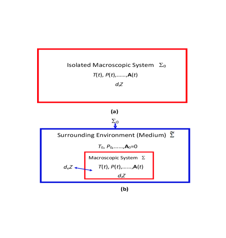
Figure 1: (a) An isolated nonequilibrium system $\Sigma_{0}$ with internally generated $d_{\text{i}}Z$ driving it towards equilibrium, during which its SI-fields $T(t),P(t),\cdots,\mathbf{A}(t)$ associated with SI-variables $S(t),V(t),\cdots,\mathbf{\xi}(t)$ continue to change towards their equilibrium values; $d_{\text{i}}Z_{k}$ denote the microanalog of $d_{\text{i}}Z$. The sign of $d_{\text{i}}Z$ is determined by the second law. (b) A nonequilibrium systen $\Sigma$ in a surrounding medium $\widetilde{\Sigma}$, both forming the isolated system $\Sigma_{0}$. The macrostates of the medium and the system are characterized by their fields $T_{0},P_{0},...,\mathbf{A}_{0}=0$ and $T(t),P(t),...,\mathbf{A}(t)$, respectively, which are different when the two are out of equilibrium. Exchange quantities ($d_{\text{e}}Z$) carry a suffix ”e” and irreversibly generated quantities ($d_{\text{i}}Z$) within the system by a suffix ”i” by extending the Prigogine notation. Their sum $d_{\text{e}}Z+d_{\text{i}}Z$ is denoted by $dZ$, which is a system-intrinsic quantity (see text). In a nonequilibrium system, the nonzero differences $F_{\text{t}}^{\text{h}}=T-T_{0}$ and $\mathbf{F}_{\text{t}}^{\text{w}}=(P-P_{0},\cdots,\mathbf{A})$ denote the set of thermodynamic forces, where we have also included the affinity $\mathbf{A}$ for internal variables $\boldsymbol{\xi}$; see text. A microstate $\mathfrak{m}_{k}$ of $\Sigma$ is specified by appending a subscript $k$ to $\mathbf{F}_{\text{t}}^{\text{w}}$ so that $\mathbf{F}_{\text{t,}k}^{\text{w}}=(P_{k}-P_{0},\cdots,\mathbf{A}_{k})$.

We have recently developed a version of nonequilibrium thermodynamics (NEQT) that is expressed in terms of only SI quantities so we have a direct access to $d_{\text{i}}Z$ and $d_{\text{i}}Z_{k}$. It has appeared in a series of papers Gujrati-I ; Gujrati-II ; Gujrati-III ; Gujrati-Entropy1 ; Gujrati-GeneralizedWork covering separate aspects, and reviewed in Gujrati-Entropy2 ; Guj-entropy-2018 . We have labeled it MNEQT to distinguish it from the M̊NEQT. It is briefly introduced in Sec. III. The theory is applicable to systems that are either isolated or in a medium within the same framework. The corresponding microstate version of the MNEQT is called the $\mu$NEQT, with $\mu$- referring to the use of SI microquantities. It is capable of studying expansion/contraction at the microstate level in interacting and isolated system that has not been possible so far as we will discuss shortly. Another reason to focus on the problem of expansion/contraction in the $\mu$NEQT is due to its close connection with Maxwell’s demon and Landauer’s eraser. Both versions of the theory also involve internal variables Maugin ; Kestin ; Prigogine ; deGroot ; Coleman that are required, see Sec. II.1, to explain nonequilibrium internal processes. Thus, they provide a very general framework of NEQT to understand a majority of nonequilibrium processes as we will explain.

We know that the classical thermodynamics is based on the concept of work and heat so we need to identify them in a NEQ process to make any progress. The central concept in the MNEQT is that of the generalized SI macrowork, see Fig. 1, $dW=P(t)dV(t)+\cdots+\mathbf{A(}t)\cdot d\mathbf{\xi(}t)$ and SI macroheat $dQ=T(t)dS(t)$, see Eq. (14), that are different from the (exchange) MI macrowork $d_{\text{e}}W=P_{0}dV(t)+\cdots$ and MI macroheat $d_{\text{e}}Q=T_{0}d_{\text{e}}S$, respectively, see Eq. (15), by irreversible contributions:

$$d_{\text{i}}W =dW-d_{\text{e}}W\geq 0,$$ (1a)

$$d_{\text{i}}Q =dQ-d_{\text{e}}Q\geq 0.$$ (1b)

The ability to directly deal with $$d_{\text{i}}W d_{\text{i}}Q dW dQ dQ=TdS S$$ and makes the MNEQT not only perfectly suited to study isolated systems as we will do, but also ensures that the generalized macrowork is isentropic and that the generalized macroheat satisfies the Clausius identity , see Eq. (14b), in all processes that we are interested in here; is always the Gibbs statistical entropy Gibbs ; Landau

$$S\doteq-{\textstyle\sum\nolimits_{k}}p_{k}\ln p_{k}.$$ (2)

The $\mu$NEQT was first introduced a while back Gujrati-GeneralizedWork and applied to a few simple examples including a brief application to the Brownian motion with a goal to compare its predictions with those from the work fluctuation theorem (WFT) due to Jarzynski Jarzynski ; see Eq. (57) for its precise formulation. The importance of microforce imbalance $\mathbf{F}_{\text{t,}k}^{\text{w}}$, see Fig. 1 caption and later, between externally applied macroforce and internally generated microforce was pointed out there for the first time. It is ubiquitous in nature Gujrati-GeneralizedWork ; Gujrati-LangevinEq as it is always present in all (EQ and NEQ) macrostates. The macroforce imbalance $\mathbf{F}_{\text{t}}=(F_{\text{t}}^{\text{h}},\mathbf{F}_{\text{t}}^{\text{w}})$ between the fields of the system and the medium, see Fig. 1 caption, determines irreversible contribution $\left(d_{\text{i}}Q,d_{\text{i}}W\right)$ and is well defined even for an isolated system. It vanishes only in EQ. This makes $\mathbf{F}_{\text{t}}$ and $\mathbf{F}_{\text{t,}k}^{\text{w}}$ central in the $\mu$NEQT, which has recently been applied Gujrati-LangevinEq to study the Brownian motion in full detail, where the relative motion of the Brownian particle with respect to the medium generates $\mathbf{F}_{\text{t,}k}^{\text{w}}$. Thus, the $\mu$NEQT is also capable of tackling small systems like Brownian particles under NEQ conditions.

I.2 Why A New Approach?

Our goal here is to use the $\mu$NEQT and the MNEQT to study general irreversible processes in interacting and isolated systems with emphasis on those undergoing phase space volume change and the resulting irreversibility at a deeper, microscopic level in terms of microstates $\left\{\mathfrak{m}_{k}\right\}$. The forthcoming demonstration of the success of our approach for free expansion, which has not been studied so far, shows its usefulness as a general theory for both interacting and isolated systems. As a general setup, we consider an interacting NEQ system $\Sigma$ in a very large medium $\widetilde{\Sigma}$, see Fig. 1(b). The two form an isolated system $\Sigma_{0}=\Sigma\cup\widetilde{\Sigma}$. Quantities pertaining to $\Sigma_{0}$ carry a suffix $0$, those pertaining to $\widetilde{\Sigma}$ carry a tilde, and those pertaining to $\Sigma$ carry no suffix. For example, the macroworks are $dW_{0},d\widetilde{W}$, and $dW$, respectively. The medium, being in EQ at all times, has no irreversibility in it so that $d_{\text{i}}\widetilde{Q}=d_{\text{i}}\widetilde{W}=0$. Because of its large size, its temperature, pressure, etc. are the same as for $\Sigma_{0}$ so they are denoted by $T_{0},P_{0}$, etc. as seen in Fig. 1(b).

The thermodynamic macroforce Prigogine ; Maugin $\mathbf{F}_{\text{t}}=(T-T_{0},P-P_{0},\cdots\mathbf{)}$ must be nonzero in a NEQ macrostate and vanish only in an EQ macrostate, i.e., when $\Sigma$ is in EQ by itself or with $\widetilde{\Sigma}$, if the latter is present. But the microforce $\mathbf{F}_{\text{t,}k}^{\text{w}}=(P_{k}-P_{0},\cdots\mathbf{)}$ is ubiquitous as noted above in all macrostates but independent of them, i.e., of $\left\{p_{k}\right\}$. Unfortunately, as we will see, this is not always enforced in many current microscopic approaches to NEQ thermodynamics.

Care must be exercised if the medium is not extremely large such as in Fig. 2.

Our methodology in the $\mu$NEQT will ensure that the microforces are always accounted for. Given $\mathbf{F}_{\text{t,}k}$, the choice of $\left\{p_{k}\right\}$ determines whether $\mathbf{F}_{\text{t}}=0$ or not so the methodology will describe thermodynamics correctly. The temporal development of $\mathfrak{M}$ in any $\mathcal{P}$ can also be studied by following the deterministic Hamiltonian evolution along Hamiltonian trajectories $\left\{\gamma_{k}\right\}$ of microstates $\left\{\mathfrak{m}_{k}\right\}$ described by its Hamiltonian $\mathcal{H}$. The trajectories, therefore, describe deterministic evolution during which $\left\{p_{k}\right\}$ does not change. As $dW$ is isentropic, the evolution involves the performance of microworks $dW_{k}$ at fixed $p_{k}$; see later. The stochasticity is due to microheat $dQ_{k}$ that modifies $p_{k}$. Thus, $dW_{k}$ and $dQ_{k}$ control different aspects of the evolution in $\mathfrak{M}$ so their combined effect completes the stochastic evolution in the $\mu$NEQT.

The trajectories have been recently popularized by modern fluctuation theorems (MFTs) Seifert ; Broeck ; see also Blau ; Ritort0 . Among these is the Jarzynski’s WFT Jarzynski , which is the most celebrated one for the simple reason that the other MFTs are related to it; see for example, Ref. Gujrati-JensenInequality . Thus, we will comment mostly on the WFT, commonly known as the JE, in the following, but the comments are equally valid for other MFTs.

There are four important and independent aspects that require careful consideration here.

(i) Internal variables. The importance of internal variables Prigogine ; Kestin ; deGroot and their affinities to describe NEQ macrostates has been well documented and is an integral part of the MNEQT and $\mu$NEQT used in this study; see also Gujrati-GeneralizedWork ; Gujrati-LangevinEq . We will give a simple argument for their relevance and the significance of affinities in Sec. II.1.

(ii) Nonequilibrium Entropy. The MI $d_{\text{e}}Z$ alone provides no insight into $d_{\text{i}}Z$ during relaxation unless SI $dZ$ is also identified. This creates a problem as $\mathfrak{M}(t)$’s denote NEQ macrostates in general so the SI $dS$ is not known if $S$ is defined only for EQ macrostates. Thus, we need to identify $S$ for NEQ macrostates. We have shown that for a NEQ system that is in internal equilibrium, the statistical entropy given in Eq. (2) is a state function in an enlarged state space involving internal variables Gujrati-I ; Gujrati-II ; see Eq. (47). It is then used in the MNEQT to determine the irreversible contributions directly. We see from Eq. (17b) that $\mathbf{F}_{\text{t}}$ is an integral part of the MNEQT as promised. We then use the MNEQT to derive the $\mu$NEQT.

(iii) Phase space volume change $\Delta\left|\Gamma\right|\neq 0$. As the number of microstates depends on $\left|\Gamma\right|$, there cannot be a one-to-one mapping between the sets of microstates in the two phase spaces in a process of expansion/contraction. The same problem arises if $d\left|\Gamma\right|/dt\neq 0$ even if at the end $\Delta\left|\Gamma\right|=0$ such as in a cyclic process.

(iv) Dissipated work. We need to provide a physical explanation of the macrowork that is being dissipated in the free expansion (see Corollary 2) and the corresponding microworks.

As interacting systems are also included in our analysis, we make a few comments in passing about the MFTs, with special attention to the WFT, that are derived for interacting systems and where trajectories are also exploited. The formulation invariably uses exchange quantities $\Delta_{\text{e}}W$ and $\Delta_{\text{e}}Q$ directly but $\Delta_{\text{i}}W$ and $\Delta_{\text{i}}Q$ are not part of the formulation. Our comments basically summarize the results already available in the literature.

The MFTs are claimed to describe NEQ processes, because of which they have attracted a lot of attention. However, despite being part of an highly active field, we find that they do not provide a useful methodology for our NEQ consideration here. There is no direct proof of for their NEQ nature that we are aware. The only indirect proof for the WFT is through the application of the Jensen’s inequality to demonstrate its compliance with the second law since the inequality leads to

$$\Delta_{\text{e}}W_{\text{J}}\leq-\Delta\overline{F},$$ (3)

where $\Delta_{\text{e}}W_{\text{J}}$ (”J” for Jarzynski’s formulation) is a particular ”average exchange” work (properly defined in Eq. (58) later) that is obtained by using the initial probability over the entire process. It turns out to be a non-thermodynamic average Gujrati-JensenInequality , and $\Delta\overline{F}$ is the difference of the equilibrium (and, therefore, thermodynamic) Helmholtz free energies in the process; see also comment (f) below in the subsection. The above inequality looks very similar to the following thermodynamic inequality involving thermodynamic average (exchange macrowork) $R=-\Delta_{\text{e}}W$, where $R$ is the exchange work $\Delta_{\text{e}}\widetilde{W}$ done by $\widetilde{\Sigma}$ on $\Sigma$,

$$R\geq\Delta\overline{F},\text{ }$$ (4)

a well-known consequence of the second law, but only if $T_{0}$ remains a constant in the process Landau . In the latter case, the dissipated work defined as

$$\Delta_{\text{diss}}W\doteq R-\Delta\overline{F}=T_{0}\Delta_{\text{i}}S\geq 0.$$ (5)

To provide an ”indirect proof” that the JE is a nonequilibrium result, Jarzynski sets without any proof that

$$\Delta_{\text{e}}W_{\text{J}}\overset{\text{conjecture}}{=}-R$$ (6)

to turn Eq. (3) into Eq. (4). However, as shown recently Gujrati-JensenInequality , Jensen’s inequality applied to the MFTs does not prove compliance with the second law inequality so $\Delta_{\text{e}}W_{\text{J}}$ in Eq. (3) cannot be equated with $\Delta_{\text{e}}W$ even when $T_{0}=$ $const$.

There are other concerns about the MFTs, which raise doubts about their usefulness for our investigation. (a) They do not include any internal variables, necessary for irreversibility; see Sec. II. (b) The external macroforce (such as the pressure $P_{0}$) is always assumed to be equal to the macroforce (such as the pressure $P$) in the system; hence, they implicitly assume that $d_{\text{e}}W=dW$, which results in $d_{\text{i}}W\equiv 0$; see Eq. (16a). This was first pointed out in Ref. Gujrati-GeneralizedWork . Thus, they do not include any thermodynamic macroforce $\mathbf{F}_{\text{t}}^{\text{w}}$ necessary for $d_{\text{i}}W$ and for irreversibility Prigogine . (c) From $d_{\text{i}}W\equiv 0$ follows $d_{\text{i}}Q\equiv 0$, see Eq. (11). If the temperature of the system is always equal to $T_{0}$, i.e., $F_{\text{t}}^{\text{h}}=T-T_{0}=0$, then it follows from Eqs. (17a, 17b) that $d_{\text{i}}S\equiv 0$. Cohen and Mauzerall Cohen0 ; Cohen00 were the first to raise concern that $T$ may not even exist for a NEQ process; see also Jarzynski-Cohen for counter-arguments, some of which we will discuss later. The concern was justified as correct later by Muschik Muschik so $T=T_{0}$ will make the MFTs unsuitable for a NEQ process. (d) MFTs are based on a fixed set of classical microstates $\left\{\mathfrak{m}_{k}\right\}$ or trajectories $\left\{\gamma_{k}\right\}$ as the use of Hamiltonian dynamics is consistently prevalent. Thus, their applicability is limited to the situation $d\left|\Gamma\right|=\Delta\left|\Gamma\right|=0$; see Sec. II.4. This was first pointed out by Sung Sung . Unfortunately, this limitation is not well recognized in the field. (e) The WFT should also apply to an isolated system JarzynskiNote . Because $d_{\text{e}}W=0$ in this case, they do not. (f) The free expansion in Fig. 2 refers to an isolated system so the WFT should be applicable in this case KestinNote , but does not as first pointed out by Sung Sung ; see also Gross ; Jarzynski-Gross for the ensuing debate. We will come back to this issue later when we discuss free expansion. (g) In addition, the averaging in the WFT is not a thermodynamic averaging over the process as first hinted by Cohen and Mauzerall Cohen0 , and established rigorously recently by us Gujrati-JensenInequality , whereas we require a thermodynamic averaging in our investigation.

Because of all these limitations, the MFTs are not of central interest to us in this study except to draw attention to the differences with our approach. Therefore, we will discuss and substantiate the above points again later in Sec. V.4 within our theoretical framework; we focus on the WFT for simplicity.

There have been several numerical attempts to study restricted expansion in an interacting system Lua0 ; Lua1 ; Baule ; Crooks-Jarzynski ; Davie ; Jarzynski1 but with a goal only to verify the WFT. Because of this, these numerical studies are also not helpful to us for the reasons stated above.

In conclusion, it is not a surprise that we are left to exclusively use the MNEQT and $\mu$NEQT in this study of interacting and isolated systems. We have already applied the MNEQT to briefly study free expansion Gujrati-Heat-Work0 ; Gujrati-Heat-Work . Here, we wish to go beyond the earlier study to demonstrate how the $\mu$NEQT can be used to study expansion/contraction with special attention to free expansion by including internal variables also. The $\mu$NEQT has also been recently applied successfully to provide a thermodynamic alternative to study Brownian motion without using the mechanical approach involving the Langevin equation Gujrati-LangevinEq . The macroscopic friction emerges as a consequence of the relative motion of the Brownian particle, an internal variable, with respect to the medium. We do not need to postulate the Langevin noise term; it emerges as a consequence of thermodynamic averaging mentioned above.

Our methodology and theory will be formulated for any arbitrary process in both interacting and isolated systems. The theory is derived from the MNEQT so it is always consistent with classical thermodynamics. The process will also include expansion and contraction as special cases but the main focus will be mostly on the spontaneous process of unrestricted, i.e., free expansion for the reason explained above. Whenever we study free expansion, we will consider the gas as a closed system $\Sigma$, which is in a medium $\widetilde{\Sigma}$ that happens to be the vacuum; see Fig. 2. Their combination forms the isolated system shown by $\Sigma_{0}$ in Fig. 1. For the set up for free expansion, we follow Kestin KestinNote as we want to make the system ($\Sigma$) and the vacuum ($\widetilde{\Sigma}$) independent. As $\widetilde{\Sigma}$ is devoid of matter and radiation, $\Sigma_{0}$ is nothing but $\Sigma$. We can replace the partition by a piston exerting an external pressure $P_{0}$ from $\widetilde{\Sigma}$ for a general expansion/contraction process. For $P_{0}<P$, the gas will expand; for $P_{0}>P$, the gas will contract. As the piston is an insulator, $\widetilde{\Sigma}$ only acts as a working medium $\widetilde{\Sigma}_{\text{w}}$. We need to bring in a thermal medium $\widetilde{\Sigma}_{\text{h}}$ to bring about thermal equilibrium. Such an expansion/contraction process is covered by the WFT Jarzynski . As $P_{0}\rightarrow 0$, and $P>0$, we obtain the limiting case of free expansion. Thus, free expansion is merely a limiting case of expansion/contraction in our approach, and does not require a separate approach. In all these cases, we require the gas particles initially to be always confined in the left chamber.

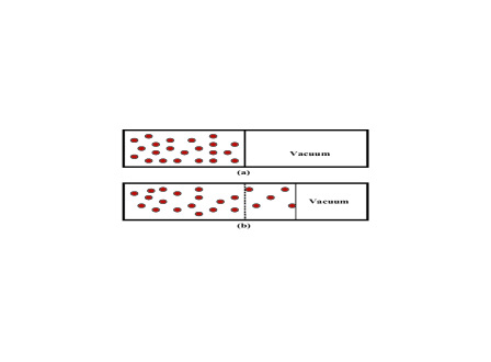
Figure 2: Free expansion of a gas. The gas is confined to the left chamber, which is separated by a hard partition (shown by a solid black vertical line) from the vacuum in the right chamber as shown in (a). At time $t=0$, the partition is removed abruptly as shown by the broken line in its original place in (b). The gas expands in the empty space, devoid of matter and radiation, on the right but the expansion is gradual as shown by the solid front, which separates it from the vacuum on its right. We can also think of the hard partition in (a) as a piston, which maintains the volume of the gas on its left. The piston can be moved slowly or rapidly to the right within the right chamber with a pressure $P_{0}<P$ to change this volume. The free expansion occurs when the piston moves extremely (infinitely) fast by letting $P_{0}\rightarrow 0$.

I.3 Layout

We briefly review some useful new concepts in the next section. We begin the discussion with the need for internal variables in a NEQ process. The nature of the parameters in the Hamiltonian of a NEQ system is discussed after that, which is then followed by the definition of Hamiltonian trajectories. We close this section by introducing the central concept of internal equilibrium. We follow this section by a brief introduction to the MNEQT in Sec. III. Here, we show the importance of internal variables for an isolated system to determine the irreversible macrowork; see Theorem 1. This partially answers one of the motivating questions. This is then followed by an introduction to the $\mu$NEQT in Sec. IV, where we introduce the concepts of various microworks and microheats. We introduce the moment generating function in Sec. V, which gives all the moments including fluctuations of microworks from this single function. We then turn to the free expansion of a classical gas and study it by restricting to use only two internal variables in the MNEQT in Sec. VI. We study the free expansion in the $\mu$NEQT in the next section. We first study it in a quantum case in Sec. VII.1 and then in the classical case in Sec. VII.2, where we introduce the important trick that allows us to consider free expansion for any arbitrary expansion. The moment generating function is used to directly demonstrate that the trick does not affect thermodynamics. The trick can be extended to a cyclic process during which the phase space volume changes nonmonotonically or to restricted expansion and contraction. A brief discussion of our results is presented in the last section.

II Basic Concepts 

II.1 Need for an Internal Variable

Consider a simple example of a NEQ system of $N$ particles, each of which can be in two levels, forming an isolated system $\Sigma$ of volume $V$. Let $\rho_{l}$ and $e_{l}(V),l=1,2$ denote the probabilities and energies of the two levels of a particle in a NEQ macrostate so that $\rho_{1},\rho_{2}$ keep changing. We have $e=\rho_{1}e_{1}+\rho_{2}e_{2}$ for the average energy per particle, which is a constant, and $d\rho_{1}+d\rho_{2}=0$ as a consequence of $\rho_{1}+\rho_{2}=1$. Using $de=0$, we get

$$d\rho_{1}+d\rho_{2}e_{2}/e_{1}=0,$$

which, for $e_{1}\neq e_{2}$, is inconsistent with the second equation (unless $d\rho_{1}=0=d\rho_{2}$, which corresponds to EQ). Thus, $e_{l}(V)$ cannot be treated as constant in determining $de$. In other words, there must be an extra dependence in $e_{l}$ so that

$$e_{1}d\rho_{1}+d\rho_{2}e_{2}+\rho_{1}de_{1}+\rho_{2}de_{2}=0,$$

and the inconsistency is removed. This extra dependence must be due to independent internal variables that are not controlled from the outside (isolated system) so they continue to relax in $\Sigma$ as it approaches EQ. Let us imagine that there is a single internal variable $\xi$ so that we can express $e_{l}$ as $e_{l}(V,\xi)$ in which $\xi$ continues to change as the system comes to equilibrium. The above equation then relates $d\rho_{1}$ and $d\xi$; they both vanish simultaneously as EQ is reached. We also see that without any $\xi$, the isolated system cannot equilibrate.

The above discussion is easily extended to a $\Sigma$ with many energy levels of a particle with the same conclusion that at least a single internal variable is required to express $e_{l}=e_{l}(V,\xi)$ for each level $l$. We can also visualize the above system in terms of microstates. A microstate $\mathfrak{m}_{k}$ refers to a particular distribution of the $N$ particles in any of different levels with energy $E_{k}={\textstyle\sum\nolimits_{l}}N_{l}e_{l}$, where $N_{l}$ is the number of particles in the $l$th level, and is obviously a function of $N,V,\xi$ so we will express it as $E_{k}(N,V,\xi)$. This makes the average energy of the system also a function of $N,V,\xi$, which we express as $E(N,V,\xi)$.

An EQ system is uniform. Thus, the presence of $\xi$ suggests some sort of nonuniformity in the system. To appreciate its physics, we consider a slightly different situation below as a possible example of nonuniformity.

We consider as a simple NEQ example a composite isolated system $\Sigma$ consisting of two identical subsystems $\Sigma_{1}$ and $\Sigma_{2}$ of identical volumes and numbers of particles but at different temperatures $T_{1}$ and $T_{2}$ at any time $t\leq\tau_{\text{eq}}$ before EQ is reached at $t=\tau_{\text{eq}}$ so the subsystems have different time-dependent energies $E_{1}$ and $E_{2}$, respectively. We assume a diathermal wall separating $\Sigma_{1}$ and $\Sigma_{2}$. Treating each subsystem in EQ at each $t$, we write their entropies as $S_{1\text{eq}}(E_{1},V/2,N/2)$ and $S_{2\text{eq}}(E_{2},V/2,N/2)$. The entropy $S$ of $\Sigma$ is a function of $E_{1},E_{2},V$, and $N$. Obviously, $\Sigma$ is in a NEQ macrostate at each $t<\tau_{\text{eq}}$. From $E_{1}$ and $E_{2}$, we form two independent combinations $E=E_{1}+E_{2}=$constant and $\xi=E_{1}-E_{2}$ so that we can express the entropy as $S(E,V,N,\xi)$. Here, $\xi$ plays the role of an internal variable, which continues to relax towards zero as $\Sigma$ approaches EQ. For given $E$ and $\xi$, $S(E,V,N,\xi)$ has the  maximum possible values since both $S_{1\text{eq}}$ and $S_{2\text{eq}}$ have their maximum value. As we will see below, this is the idea behind the concept of internal equilibrium in which $S(E,V,N,\xi)$ is a state function of state variables and continues to increase as $\xi$ decreases and vanishes in EQ.

We assume $\Sigma$ to be in IEQ at each $t$ in this simple example. From $1/T=\partial S/\partial E$ and $A/T=\partial S/\partial\xi$, $A$ being the activity associated with $\xi$, we find that

$$T=2T_{1}T_{2}/(T_{1}+T_{2}),A=(T_{2}-T_{1})/(T_{1}+T_{2}).$$

As EQ is attained, $T\rightarrow T_{\text{eq}}$, the EQ temperature of both subsystems and $A\rightarrow A_{0}=0$ as expected. We see that in this simple example $Ad\xi/T$ is the contribution due to irreversiblity in $dS$, which also shows that $(-Ad\xi)$ is the contribution due to irreversiblity in $dE$.

In general, the activity $\mathbf{A}$ controls the behavior of $\boldsymbol{\xi}$ in a NEQ macrostate and vanishes when EQ is reached. Here, we will take a more general view of $\mathbf{A}$, and extend its definition to $\mathbf{X}$ also Gujrati-I . Comparing $A$ with $F_{\text{t}}^{\text{h}}$, we clearly see that $F_{\text{t}}^{\text{h}}$ also plays the role of an activity. The same reasoning also shows that $\mathbf{F}_{\text{t}}^{\text{w}}$ plays the role of an activity.

The example can be easily extended to the case of expansion and contraction by replacing $E,E_{1}$, and $E_{2}$ by $N,N_{\text{L}}$, and $N_{\text{R}}$, see Fig. 2, to describe the diffusion of particles. The role of $\beta$ and $E$, etc. are played by $\beta\mu$ and $N$, etc.

II.2 Hamiltonian with Internal Variables

It is clear that in order to capture a NEQ process, internal variables are necessary. Another way to appreciate this fact is to realize that for an isolated system, all the observables in $\mathbf{X=(}E,V,N,\cdots\mathbf{)}$ are fixed so if the entropy is a function of $\mathbf{X}$ only, it cannot change Gujrati-I ; Gujrati-II ; Guj-entropy-2018 ; Gujrati-Entropy1 ; Gujrati-Entropy2 . Thus, we need additional independent variables to ensure the law of increase of entropy for a NEQ system. An EQ macrostate is represented by a point in the state space $\mathfrak{S}_{0}$ spanned by $\mathbf{X}$, but a NEQ macrostate by a point in an enlarged state space $\mathfrak{S}$ spanned by $\mathbf{Z\doteq}(\mathbf{X,}\boldsymbol{\xi})$, where $\boldsymbol{\xi}$ is the set formed by internal variables. Internal variables cannot be controlled from the outside of the system; they are only controlled by the processes within the system. On the other hand, the observables in $\mathbf{X}$ are controlled from the outside. We will call $\mathbf{X}$ a set of observables and $\mathbf{Z}$ a set of state variables. In EQ, internal variables are no longer independent of the observables. Consequently, their affinities (see later) vanish in EQ. It is common to define the internal variables so their EQ values vanish.

As we will be dealing with the Hamiltonian of the system, it is useful to introduce the sets $\mathbf{X}^{E}\doteq\mathbf{X\backslash}E=(V,N,\cdots)$, and $\mathbf{Z}^{E}\doteq\mathbf{Z\backslash}E=(V,N,\cdots,\boldsymbol{\xi})=(\mathbf{X}^{E}\mathbf{,}\boldsymbol{\xi})$. Then, $E$ and $E_{k}$ become a function of $\mathbf{Z}^{E}$ as we saw in Sec. II.1. Here, $\mathbf{Z}^{E}$ appears as a parameter in the Hamiltonian, which we will write as $\mathcal{H}(\left.\mathbf{z}\right|\mathbf{Z}^{E})$, where $\mathbf{z}$ is a point (collection of coordinates and momenta of the particles) in the phase space $\Gamma(\mathbf{Z}^{E})$ specified by $\mathbf{Z}^{E}$. As an example, $N,V$, and $\xi$ are the parameters in the previous section. When the system moves about in the phase space $\Gamma(\mathbf{Z}^{E})$, $\mathbf{z}$ changes but $\mathbf{Z}^{E}$ as a parameter remains fixed in a state subspace $\mathfrak{S}^{E}\doteq\mathfrak{S}\mathbf{\backslash}E$.

II.3 Hamiltonian Trajectories

Traditional formulation of statistical thermodynamics Landau ; Gibbs ; Gujrati-Symmetry takes a mechanical approach in which $\mathfrak{m}_{k}$ follows its classical or quantum mechanical evolution dictated by its SI Hamiltonian $\mathcal{H}(\left.\mathbf{z}\right|\mathbf{Z}^{E})$. The quantum microstates are specified by a set of good quantum numbers, which we have denoted by $k$ above as a single quantum number for simplicity; we take $k\in\mathbb{N},\mathbb{N}$ denoting the set of natural numbers. We will see below that $k$ does not change as $\mathbf{Z}^{E}$ changes. In the classical case, we can use a small cell $\delta\mathbf{z}_{k}$ of size $(2\pi\hbar)^{3N}$ around $\mathbf{z}_{k}=\mathbf{z}$ as the microstate $\mathfrak{m}_{k}$. In the rest of the work, we will keep $N$ fixed to fix the size of the system. Therefore, from now on, $\mathbf{X}$ and $\mathbf{Z}$ will not contain it. The Hamiltonian gives rise to a purely mechanical evolution of individual $\mathfrak{m}_{k}$’s, which we will call the Hamiltonian evolution, and suffices to provide their mechanical description. The change in $\mathcal{H}(\left.\mathbf{z}\right|\mathbf{Z}^{E})$ in a process is

$$d\mathcal{H}=\frac{\partial\mathcal{H}}{\partial\mathbf{z}}\cdot d\mathbf{z}+\frac{\partial\mathcal{H}}{\partial\mathbf{Z}^{E}}\cdot d\mathbf{Z}^{E}.$$ (7a)

The first term on the right vanishes identically due to Hamilton’s equations of motion for any $$\mathfrak{m}_{k} \mathbf{Z}^{E} E_{k}=\mathcal{H}_{k}\doteq\mathcal{H}(\left.\mathbf{z}_{k}\right|\mathbf{Z}^{E}) \mathfrak{m}_{k} \Gamma(\mathbf{Z}^{E}) d\mathbf{Z}^{E} \mathfrak{S} E_{k} \mathbf{z}_{k} \mathcal{H}(\left.\mathbf{z}\right|\mathbf{Z}^{E}) \mathfrak{S}$$. Thus, for fixed , the energy remains constant as moves about in . Only the variation in generates any change in . Consequently, we do not worry about how  changes in in the phase space, and focus, instead, on the state space , in which can write

$$dE_{k}=\frac{\partial E_{k}}{\partial\mathbf{Z}^{E}}\cdot d\mathbf{Z}^{E}=-dW_{k},$$ (7b)

where $$dW_{k} \mathbf{F}_{k}^{E}$$ denotes the generalized microwork produced by the generalized microforce :

$$dW_{k}=\mathbf{F}_{k}^{E}\cdot d\mathbf{Z}^{E},\ \mathbf{F}_{k}^{E}\doteq-\partial E_{k}/\partial\mathbf{Z}^{E}.$$ (7c)

We can now identify $$\mathbf{Z}^{E} d\mathbf{Z}(t)\doteq(dE(t),d\mathbf{Z}^{E}(t)) \mathfrak{S} \left\{dW_{k}\right\} \mathcal{P} \gamma_{k} \mathfrak{S} \mathfrak{m}_{k} \mathbf{Z}^{E} \mathbf{Z}_{\text{in}}^{E} \mathbf{Z}_{\text{fin}}^{E} \mathcal{P} dW_{k} p_{k} dW_{k} dW_{k} k \mathfrak{m}_{k}$$ as the work parameter, whose variation in defines not only the microworks , but also a thermodynamic process . The trajectory in followed by as a function of time will be called the Hamiltonian trajectory during which varies from its initial (in) value  to its final (fin) value during . The variation produces the generalized microwork ; plays no role so is purely mechanical, which simplifies its determination in our theory. The microwork also does not change the index of as said above.

Being purely mechanical in nature, a trajectory is completely deterministic and cannot describe the evolution of a macrostate $\mathfrak{M}$ during $\mathcal{P}$ unless supplemented by thermodynamic stochasticity, which requires $p_{k}(\mathfrak{M})$ as discussed above Landau , and is related to $dQ_{k}$ as shown later; see Eq. (38). Thermodynamics emerges when quantities pertaining to the trajectories are averaged over the trajectory ensemble $\left\{\gamma_{k}\right\}$ with appropriate probabilities that will usually change during the process. In this sense, our approach is different from approaches using stochastic trajectories Seifert ; Broeck , where $dE_{k}$ is identified with the exchange microwork $dR_{k}\doteq-d_{\text{e}}W_{k}$; see Remark 6.

The development of the $\mu$NEQT requires pursuing individual trajectory $\gamma_{k}$ of $\mathfrak{m}_{k}(\mathbf{Z}^{E})$. In the following, $\mathfrak{m}_{k}$ will usually stand for classical microstates unless specified otherwise, and follows its deterministic trajectory $\gamma_{k}$ as $\mathfrak{m}_{k\text{,in}}\doteq\mathfrak{m}_{k}(\mathbf{Z}_{\text{in}}^{E})$ evolves into $\mathfrak{m}_{k\text{,fin}}\doteq\mathfrak{m}_{k}(\mathbf{Z}_{\text{fin}}^{E})$. By reversing the change in $\mathbf{Z}^{E}$ from $\mathbf{Z}_{\text{fin}}^{E}$ to $\mathbf{Z}_{\text{in}}^{E}$, $\mathfrak{m}_{k}(\mathbf{Z}_{\text{fin}}^{E})$ comes back to $\mathfrak{m}_{k}(\mathbf{Z}_{\text{in}}^{E})$. Thus, $\gamma_{k}$ defines an identity map $\mathcal{T}:$

$$\mathcal{T}:\mathfrak{m}_{k}(\mathbf{Z}_{\text{in}}^{E})\rightleftarrows\mathfrak{m}_{k}(\mathbf{Z}_{\text{fin}}^{E})$$ (8)

without altering the index $k$ so it is a one-to-one ($1$-to-$1$) or identity mapping of microstates. The two arrows mean that the mapping can be inverted without altering the index $k$ so it is a one-to-one ($1$-to-$1$) or identity mapping of microstates.

II.4 Phase Space Volume Change

However, Hamiltonian trajectories for classical microstates are not suitable for processes that involve expansion and contraction in the volume $V$ and/or other parameters in $\mathbf{Z}^{E}$ of the system with a corresponding change in the phase space volume $\left|\Gamma\right|$. In the following, we will think of $V$ as the varying work parameter for simplicity. Then, during expansion, the initial volume $\left|\Gamma\right|_{\text{in}}\doteq\left|\Gamma(\mathbf{Z}_{\text{in}}^{E})\right|$ is smaller than the final volume $\left|\Gamma^{\prime}\right|_{\text{fin}}\doteq\left|\Gamma(\mathbf{Z}_{\text{fin}}^{E})\right|$ as shown in Fig. 3. This means that there are microstates such as $\delta\mathbf{\zeta}^{\prime}$ ($\neq\delta\mathbf{z}^{\prime}$) in $\Gamma_{\text{fin}}^{\prime}\doteq\Gamma(\mathbf{Z}_{\text{fin}}^{E})$ that cannot be reached from any of the microstate $\delta\mathbf{z}$ in $\Gamma_{\text{in}}\doteq\Gamma(\mathbf{Z}_{\text{in}}^{E})$ along Hamiltonian trajectories; the latter take $\delta\mathbf{z}$ into $\delta\mathbf{z}^{\prime}$ inside the broken horizontal ellipse. The converse is true for contraction.

Note also that we are not interested in the cardinality of the initial and final sets of microstates $\left\{\mathfrak{m}_{\text{in}}\right\}$ and $\left\{\mathfrak{m}_{\text{fin}}\right\}$,respectively. We are interested in how they map under Hamiltonian evolution; see Sec. VIII for more clarification.

It is clear that in the classical case, we require a new approach to overcome the loss of the $1$-to-$1$ mapping if we confine ourselves to only Hamiltonian trajectories. To the best of our knowledge, the problem of how to overcome this hurdle of phase space volume change using Hamiltonian trajectories has not been solved.

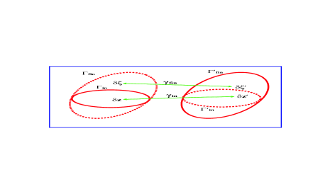
Figure 3: The evolution of a microstate $\delta\mathbf{z}\in\mathbf{\Gamma}_{\text{in}}$ into $\delta\mathbf{z}^{\prime}\in\mathbf{\Gamma}_{\text{fin}}^{\prime}$ following the variation in $\mathbf{Z}^{E}$ (green arrows). The initial and final phase spaces are $\mathbf{\Gamma}_{\text{in}}$ and $\mathbf{\Gamma}_{\text{fin}}^{\prime}$ shown by the interiors of the red solid ellipses. By changing $\mathbf{Z}^{E}$ in the reverse order maps $\delta\mathbf{z}^{\prime}$ into $\delta\mathbf{z}$ as implied by the reverse green arrows. The microstates $\delta\mathbf{\zeta}^{\prime}$ and $\delta\mathbf{\zeta}$, and other quantities are explained in the text.

We overcome the hurdle by introducing a novel but simple trick. The clue for the new approach comes from considering trajectories in quantum mechanics. As quantum microstates form a denumerable set with index $k\in\mathbb{N}$ as $\mathbf{Z}^{E}$ changes, there is a $1$-to-$1$ mapping  as in Eq. (8) between $\mathfrak{m}_{k\text{,in}}$ and $\mathfrak{m}_{k\text{,fin}}$ during expansion and contraction, which helps us remedy the lack of one-to-one correspondence due to volume change in the classical case. The trick is to enlarge the smaller phase space to become equal to the larger phase space by adding missing microstates that appear with nonzero but vanishingly small probabilities. As the work along deterministic trajectories in Eq. (7b) is oblivious to their probabilities (even though they continue to change in thermodynamics), we can add trajectories initiating at the missing microstates to obtain a enlarged $1$-to-$1$ trajectory ensemble $\left\{\gamma\right\}$. At the end of the computation of ensemble averages, a formal limit of vanishing probabilities of missing initial microstates is taken.

II.5 Internal Equilibrium (IEQ)

The central concept of the NEQT exploited here is that of the internal equilibrium (IEQ) according to which the entropy $S$ of a NEQ macrostate is a state function of the state variables in the enlarged state space $\mathfrak{S}$ Gujrati-I ; Gujrati-II ; Gujrati-III relative to the EQ state space $\mathfrak{S}_{0}$ due to independent internal variables Coleman ; deGroot ; Prigogine ; Maugin ; Gujrati-I ; Gujrati-II that are required to describe a NEQ macrostate as explained above. In EQ, the internal variables are no longer independent of the observables forming the space $\mathfrak{S}_{0}$. As a consequence, their affinities vanish in EQ. In general, the temperature $T$ of the system in IEQ is identified in the standard manner by the relation

$$1/T=\partial S/\partial E$$ (9)

using the fact that $S$ is state function in $\mathfrak{S}$.

An important property of IEQ macrostates is the following: It is possible in an IEQ macrostate to have different degrees of freedom or different parts of a system to have different temperatures than $T$. For example, in a glass, it is well known that the vibrational degrees of freedom have a different temperature than the configurational degrees of freedom Debenedetti ; Gujrati-Hierarchy . In the viscous drag problem, the CM-motion of the Brownian particle can have a different temperature than $T$ of the rest of the particles in the fluid Gujrati-LangevinEq . This observation is easily verified in MNEQT based on the concept of IEQ as done elsewhere (Gujrati-Hierarchy, , see Sec. 8.1 and Eq. (58)). By taking a larger and larger set of internal variables, we can treat almost all NEQ macrostates as if in IEQ. Thus, the MNEQT is an extremely useful thermodynamics for NEQ systems.

III The MNEQT

An EQ macrostate is described by $\mathbf{X=(}E,V,\cdots\mathbf{)}$, and its entropy is a state function $S(\mathbf{X})$. Away from EQ, $S(\mathbf{Z})$ becomes a state function for NEQ macrostates in IEQ. In the following, we will focus on $V$ and $\xi$ as members of $\mathbf{Z}^{E}\doteq\mathbf{Z\backslash}E$ for simplicity but the discussion is general and applies to any $\mathbf{Z}^{E}$. Indeed, we use two internal variables when we study free expansion. The microstate $\mathfrak{m}$ follows its evolution dictated by its (SI) Hamiltonian $\mathcal{H}(\left.\mathbf{z}\right|V,\boldsymbol{\xi})$; the interaction with $\widetilde{\Sigma}$ is usually treated as a very weak stochastic perturbation, which immediately suggests adopting a SI description.

III.1 Macrowork and Macroheat

There are two kinds of macrowork,the SI and MI macroworks $dW$ and $d_{\text{e}}W$, respectively, in NEQT; see Eq. (1a). The irreversible macrowork $d_{\text{i}}W\geq 0$ vanishes only for a reversible process. We similarly have two kinds of macroheat, the SI macroheat $dQ$ and the MI exchange macroheat $d_{\text{e}}Q$; see Eq. (1b). The irreversible heat $d_{\text{i}}Q\geq 0$ vanishes only for a reversible process. The first law can be equivalently expressed in terms of SI and MI quantities, respectively:

$$dE =dQ-dW,$$ (10a)

$$dE =d_{\text{e}}Q-d_{\text{e}}W;$$ (10b)

the first equation follows from Eq. (31a) and the discussion following it. From the above two equations follows the important identity

$$d_{\text{i}}Q\equiv d_{\text{i}}W,$$ (11)

which establishes that internal processes ensure that irreversible macroheat and macrowork within $\Sigma$ are identically equal in magnitude. This equality is very general and will be used extensively in this study. It is a consequence of a very general result of NEQT that no irreversible process can generate any internal change in the (average) energy of the system, i.e.,

$$d_{\text{i}}E\equiv 0,$$ (12)

so that $d_{\text{e}}E=dE$. From now on, we will refer to $dW$ and $dQ$ ($d_{\text{e}}W$ and $d_{\text{e}}Q$) simply as macrowork and macroheat (exchange macrowork and exchange macroheat), respectively, so no confusion can arise.

The discussion above is valid for any arbitrary process, but, from now on, we restrict to the case when $S=S(\mathbf{Z})$ is a state function in $\mathfrak{S}$ for simplicity, i.e., for the macrostate to be an IEQ macrostate Gujrati-I ; Gujrati-II to define $T$. The discussion to an arbitrary process, which can be done, will be avoided here.

For a process requiring pressure-volume macrowork only, we have $dW=PdV$ done by $\Sigma$ (SI) or $d\widetilde{W}=-P_{0}dV$ done by $\widetilde{\Sigma}$ (MI) in terms of the instantaneous pressure $P=-\partial E/\partial V$ of $\Sigma$ or $P_{0}~{}$of $\widetilde{\Sigma}$, and their volume change $dV$ or $-dV$, respectively. The exchange macrowork is $d_{\text{e}}W=-d\widetilde{W}=P_{0}dV$. For irreversibility, $P\neq P_{0}$, with $P-P_{0}$ playing the role of an activity Gujrati-I . The irreversible or dissipated work is $d_{\text{i}}W=(P-P_{0})dV$ Kestin ; Woods ; Prigogine .

Comparing Eq. (10a) for an IEQ macrostate with

$$dS=(\partial S/\partial\mathbf{X})\cdot d\mathbf{X+}(\partial S/\partial\boldsymbol{\xi})\cdot d\boldsymbol{\xi},$$ (13)

allows us to identify the macroheat and macrowork as

$$dW =T(\partial S/\partial\mathbf{Z}^{E})\cdot d\mathbf{Z}^{E}=PdV+\cdots+\mathbf{A}\cdot d\boldsymbol{\xi},$$ (14a)

$$dQ =TdS\boldsymbol{;}$$ (14b)

where $$T\doteq 1/(\partial S/\partial E)=1/\beta, \beta\mathbf{A}\doteq(\partial S/\partial\boldsymbol{\xi}) \mathbf{A} \cdots \mathbf{X} \widetilde{\Sigma} T=T_{0},P=P_{0},\cdots,\mathbf{A}_{0}=0$$ identifies the affinity , and refers to other elements in . Recalling that for , , we have in general,

$$d_{\text{e}}W =-d\widetilde{W}=P_{0}dV+\cdots,$$ (15a)

$$d_{\text{e}}Q =-d\widetilde{Q}=T_{0}d_{\text{e}}S.$$ (15b)

We can identify the irreversible macrowork due to $$\mathbf{F}_{\text{t}}^{\text{w}}$$:

$$d_{\text{i}}W=(P-P_{0})dV+\cdots+\mathbf{A}\cdot d\boldsymbol{\xi=}\mathbf{F}_{\text{t}}^{\text{w}}\cdot d\mathbf{Z}^{E}\geq 0,$$ (16a)

where

$$\mathbf{F}_{\text{t}}^{\text{w}}=\left\{P-P_{0},\cdots,\mathbf{A}=\mathbf{A-A}_{0}\right\}$$ (16b)

is the thermodynamic force, which also include the affinity $$\mathbf{A} d_{\text{i}}W\rightarrow 0 \mathbf{F}_{\text{t}}^{\text{w}}\rightarrow 0 d_{\text{i}}W>0 \mathbf{F}_{\text{t}}^{\text{w}} (P-P_{0})dV,\cdots,A_{1}d\xi_{1},A_{2}d\xi_{2},\cdots \mathbf{F}_{\text{t}}^{\text{w}}\cdot d\mathbf{Z}^{E}$$, driving the system towards EQ when as . For irreversibility, , which requires to be non-zero as asserted earlier in Sec. I.1. Each component of  must be positive separately for irreversibility.

Using $d_{\text{e}}Q=T_{0}d_{\text{e}}S$ in Eq. (14b), we find

$$d_{\text{i}}Q=\left\{\begin{array}[c]{c}(T-T_{0})d_{\text{e}}S+Td_{\text{i}}S\\ (T-T_{0})dS+T_{0}d_{\text{i}}S\end{array}\right.\geq 0.$$ (17a)

Using $$d_{\text{i}}Q=d_{\text{i}}W$$ and Eq. (16a), we also obtain

$$d_{\text{i}}S=\left\{\begin{array}[c]{c}\left\{(T_{0}-T)d_{\text{e}}S+\mathbf{F}_{\text{t}}^{\text{w}}\cdot d\mathbf{Z}^{E}\right\}/T\\ \left\{(T_{0}-T)dS+\mathbf{F}_{\text{t}}^{\text{w}}\cdot d\mathbf{Z}^{E}\right\}/T_{0}\end{array}\right.\geq 0.$$ (17b)

We see that $$F_{\text{t}}^{\text{h}}=T_{0}-T F_{\text{t}}^{\text{h}}d_{\text{e}}S\geq 0 d_{\text{i}}S d_{\text{e}}S=0 T=T_{0}$$ can also be thought of as a ”thermodynamic force” due to thermal imbalance driving the system towards EQ via heat transfer; it ensures that , in accordance with the second law. Thus, both contributions to are always nonnegative as expected. In the absence of any heat exchange () or for an isothermal system (),  we have

$$d_{\text{i}}Q=Td_{\text{i}}S=d_{\text{i}}W,$$ (18)

where $d_{\text{i}}W$ is given by Eq. (16a).

We can use

$$\mathbf{F}_{\text{t}}\doteq(F_{\text{t}}^{\text{h}},\mathbf{F}_{\text{t}}^{\text{w}})$$ (19)

as the generalized thermodynamic force, which includes the thermal imbalance $F_{\text{t}}^{\text{h}}$ and the work imbalance $\mathbf{F}_{\text{t}}^{\text{w}}$. It should be obvious that $F_{\text{t}}^{\text{h}}$ is meaningless for an isolated or an isothermal system, while $\mathbf{F}_{\text{t}}^{\text{w}}$ is meaningful for all NEQ systems, interacting or not.

III.2 Internal Variables and the Isolated System

The above formulation of MNEQT is perfectly suited for considering an isolated system $\Sigma$ ($d_{\text{e}}W=d_{\text{e}}Q\equiv 0$) so that Eqs. (11-12) becomes the most important thermodynamic equality. For an isolated system, $d\mathbf{X}=0$ so that $d_{\text{i}}W=\mathbf{A}\cdot d\boldsymbol{\xi}$ as seen from Eq. (16a).

Theorem 1

The irreversible entropy generated within an isolated system is still related to the dissipated work performed by the internal variables.

Proof. As $E$ remains fixed for an isolated system ($dQ=Td_{\text{i}}S$), we have from Eq. (10a)

$$Td_{\text{i}}S=d_{\text{i}}W=\mathbf{A}\cdot d\boldsymbol{\xi}\geq 0$$ (20)

in accordance with the second law.   

Note that the above equation, though it is identical to Eq. (18) in form, is very different in that $d_{\text{i}}W$ here is simply $\mathbf{A}\cdot d\boldsymbol{\xi}$ and not the full expression in Eq. (16a). Same conclusion is also obtained when we apply Eq. (17b) to an isolated system.

The above theorem thus clarifies the unsettling fact about the significance of dissipated macrowork that motivated this study; see also Eq. (26). The dissipated macrowork $d_{\text{i}}W$ in an isolated system is performed by the internal variable $\boldsymbol{\xi}$, and can be identified with $d_{\text{i}}S$ as noted in Sec. I.1.

Corollary 2

Neither the entropy can increase nor will there be any dissipated work unless some internal variables are present in an isolated system. If no internal variables are used to describe an isolated system, then thermodynamics requires it to be in EQ.

Proof. The proof follows trivially from Eq. (20).   

III.3 Cumulative Macroquantities in a Thermodynamic Process

Let us consider a thermodynamic process $\mathcal{P}$ between two macrostates $\mathfrak{M}_{\text{in}}\doteq\mathfrak{M}(T_{\text{in}},\mathbf{Z}_{\text{in}}^{E})$ and $\mathfrak{M}_{\text{fin}}\doteq\mathfrak{M}(T_{\text{fin}},\mathbf{Z}_{\text{fin}}^{E})$ at temperatures $T_{\text{in}}$ and $T_{\text{fin}}$, respectively. The system may be isolated and in IEQ so its temperature is well defined. It may be very different from the temperature $T_{0}$ of the medium, if $\Sigma$ is not isolated. In each case, the cumulative macroquantities of $\Sigma$ are obtained by simple integration along the process:

$$\Delta_{\alpha}E ={\textstyle\int\nolimits_{\mathcal{P}}}d_{\alpha}E,\Delta_{\alpha}S={\textstyle\int\nolimits_{\mathcal{P}}}d_{\alpha}S,$$ (21a)

$$\Delta_{\alpha}W ={\textstyle\int\nolimits_{\mathcal{P}}}d_{\alpha}W,\Delta_{\alpha}Q={\textstyle\int\nolimits_{\mathcal{P}}}d_{\alpha}Q.$$ (21b)

Similar definitions also apply to $$\widetilde{\Sigma} \Sigma_{0} d_{\alpha}=d,d_{\text{e}} d_{\text{i}}$$ and . Above we have used the compact notation , and to indicate various infinitesimal forms, which we can treat as linear operators. They will be useful in the rest of the work.

We now consider an interacting system and determine $\Delta W$ between two EQ macrostates $\mathfrak{M}_{\text{in,eq}}\doteq\mathfrak{M}(T_{0},\mathbf{Z}_{\text{in}}^{E})$ and $\mathfrak{M}_{\text{fin,eq}}\doteq\mathfrak{M}(T_{0},\mathbf{Z}_{\text{fin}}^{E})$ at the same temperature. We denote the corresponding process by $\mathcal{P}_{0}$, which may possibly be irreversible. We recall that the Helmholtz free energy

$$\overline{F}=E-T_{0}S$$ (22a)

(conventionally written as $$F T_{0} T \overline{F} F$$ but we will use that for a SI free energy here) is also the Helmholtz free energy of a NEQ system Gujrati-I in a canonical ensemble in a medium at temperature ; the temperature of the system does not appear in explicitly. It is this free energy that follows the second law Gujrati-I and not , which is the SI free energy

$$F=E-TS+\mathbf{A}\cdot\boldsymbol{\xi.}$$ (22b)

It depends only on the system and is very different from $$\overline{F} \Delta\overline{F} \Delta W=\Delta Q-\Delta E=\Delta Q-\Delta\overline{F}-\Delta(T_{0}S)$$. It will be useful later. In terms of the difference for the two macrostates, we have . Thus,

$$\Delta W ={\textstyle\int\nolimits_{\mathcal{P}}}[(T-T_{0})dS-SdT_{0}]-\Delta\overline{F},$$ (23a)

$$\Delta_{\text{e}}W =-{\textstyle\int\nolimits_{\mathcal{P}}}[T_{0}d_{\text{i}}S+SdT_{0}]-\Delta\overline{F},$$ (23b)

$$\Delta_{\text{i}}W ={\textstyle\int\nolimits_{\mathcal{P}}}[TdS-T_{0}d_{\text{e}}S]$$ (23c)

The corresponding infinitesimal form is

$$dW =(T-T_{0})dS-SdT_{0}-d\overline{F},$$ (24a)

$$d_{\text{e}}W =-[T_{0}d_{\text{i}}S+SdT_{0}]-d\overline{F},$$ (24b)

$$d_{\text{i}}W =TdS-T_{0}d_{\text{e}}S.$$ (24c)

If the medium is maintained at a fixed temperature during $$\mathcal{P} dT_{0}$$, we must remove the term above.

We see that if and only if $T=T_{0}=const$ over the entire process $\mathcal{P}$ so that it is isothermal, we have

$$\Delta W_{\text{isoth}}=-\Delta\overline{F},\Delta_{\text{e}}W_{\text{isoth}}=-T_{0}\Delta_{\text{i}}S-\Delta\overline{F},$$ (25a)

in terms of the Helmholtz free energy difference so that

$$\Delta_{\text{i}}W_{\text{isoth}}=T_{0}\Delta_{\text{i}}S.$$ (25b)

This is a very strong requirement when $$\widetilde{\Sigma} \Sigma d_{\text{i}}Q=T_{0}d_{\text{i}}S \Delta_{\text{i}}Q=T_{0}\Delta_{\text{i}}S$$ remains in continuous contact with , since it requires complete thermal equilibrium at all times. In this case, and ; see also Eq. (18).

We now consider an isolated system for which $\Delta E=0$ so that

$$\Delta_{\text{i}}W={\textstyle\int\nolimits_{\mathcal{P}}}Td_{\text{i}}S=T_{0}\Delta_{\text{i}}S+{\textstyle\int\nolimits_{\mathcal{P}}}[(T-T_{0})d_{\text{i}}S\geq 0,$$ (26)

which is in accordance with Theorem 1 and finally explains the physical meaning of the irreversible macrowork, which was one of the questions that had prompted this investigation. It should be clear that the derivation is not restricted to a process between two EQ macrostates.

III.4 A Simple Study Case

As remarked earlier, we use a single internal variable $\xi$ in addition to $V$ for $\mathbf{Z}^{E}$ for simplicity so that we have

$$dW=PdV+Ad\xi,d_{\text{e}}W=P_{0}dV.$$ (27a)

The dissipated work is

$$d_{\text{i}}W=(P-P_{0})dV+Ad\xi\geq 0;$$ (27b)

in the absence of $$\xi$$. We also have

$$Td_{\text{i}}S=(T-T_{0})d_{\text{e}}S+(P-P_{0})dV+Ad\xi\geq 0,$$ (28)

where we have used $d_{\text{i}}Q=d_{\text{i}}W$. If no exchange macrowork is done, $dV=0$ and $Td_{\text{i}}S=(T-T_{0})d_{\text{e}}S+Ad\xi\geq 0$. In the absence of any exchange macroheat, we have $Td_{\text{i}}S=(P-P_{0})dV+Ad\xi\geq 0$. In an isolated system, we have

$$Td_{\text{i}}S=Ad\xi\geq 0,$$ (29)

which is a special case of the general result in Eq. (20).

IV The $\mu$NEQT

We will closely follow Refs. Gujrati-GeneralizedWork ; Gujrati-LangevinEq to provide a brief pedagogical review of the $\mu$NEQT for the sake of continuity and demonstrate its successful application to the free expansion, which has not been attacked by any other approach so far. The main idea is to cast any macroquantity in the MNEQT as a thermodynamic average, see Eq. (30a), over microstates. Then, we can identify corresponding microquantities. Some care must be exercised to ensure their uniqueness as we will see. These microstate microquantities can be used to identify the contribution along a trajectory by simple integration.

IV.1 General Setup

The theory was first presented in a very condensed form in Ref. Gujrati-GeneralizedWork . It was successfully applied Gujrati-LangevinEq to provide an alternative, but a much simpler, approach (using deterministic microforces $\mathbf{F}_{k}^{E}$) to study Brownian motion without the use of Langevin’s stochastic noise term so it does not require the use of the stochastic theory. The microforce responsible for the Brownian motion is associated with the relative motion of the center of mass of the Brownian particle with respect to the medium. A good description of the salient features of the $\mu$NEQT is available there.

It follows from $\mathcal{H}(\left.\mathbf{z}\right|\mathbf{Z}^{E})$ that $E_{k}$ also depend on $\mathbf{Z}^{E}$. A macroquantity $O$ (except the temperature) in the MNEQT appear as a thermodynamic average $\left\langle O\right\rangle$ over $\left\{\mathfrak{m}_{k}\right\}$:

$$O=\left\langle O\right\rangle\doteq{\textstyle\sum\nolimits_{k}}p_{k}O_{k},$$ (30a)

where $$O_{k} O \mathfrak{m}_{k}$$ is the value of associated with . Thus,

$$E={\textstyle\sum\nolimits_{k}}p_{k}E_{k},P={\textstyle\sum\nolimits_{k}}p_{k}P_{k},S={\textstyle\sum\nolimits_{k}}p_{k}S_{k},$$ (30b)

etc. Here, $$E_{k},P_{k}\doteq-\partial E_{k}/\partial V,S_{k}\doteq-\ln p_{k} \mathfrak{m}_{k} p_{k} S_{k} \mathfrak{m}_{k} {\textstyle\sum\nolimits_{k}}p_{k}=1$$, etc. are the values that are only determined by . However, or , although associated with  is not determined by it alone because of the constraint , which makes it depend on the macrostate also.

From $E$, we have the change in the macroenergy

$$dE={\textstyle\sum\nolimits_{k}}E_{k}dp_{k}+{\textstyle\sum\nolimits_{k}}p_{k}dE_{k}$$ (31a)

between two neighboring macrostates. We will use the compact notation

$$dE_{\text{h}} \doteq{\textstyle\sum\nolimits_{k}}E_{k}dp_{k}=\left\langle Ed\eta\right\rangle,$$

$$dE_{\text{w}} \doteq{\textstyle\sum\nolimits_{k}}p_{k}dE_{k}=\left\langle dE\right\rangle,$$ (32)

where we have introduced $\eta_{k}\doteq\ln p_{k}$ so that $d\eta_{k}=dp_{k}/p_{k}$. As $\left\{E_{k}\right\}$ does not change but $\left\{p_{k}\right\}$ changes in $dE_{\text{h}}$, it must depend on $dS$; see Eq. (14b). As $\left\{p_{k}\right\}$ is not changed in $dE_{\text{w}}$, it is evaluated at fixed entropy $S$ Gujrati-Heat-Work0 ; Gujrati-Entropy2 . Comparing $dE$ with the first law in Eq. (10a), we identify

$$dQ =dE_{\text{h}}\doteq\left\langle Ed\eta\right\rangle,$$ (33a)

$$dW =-dE_{\text{w}}\doteq-\left\langle dE\right\rangle$$ (33b)

Thus, the generalized macroheat $$dQ dS dW F_{\text{t}}^{\text{h}} \mathbf{F}_{\text{t}}^{\text{w}}$$ is a contribution proportional to and the generalized macrowork is an isentropic contribution as noted in Sec. I.1. The identification of macroheat and macroworks above also explains the choice of h for heat and w for work as suffix above and superfix in and .

We can now identify the (generalized) microheat and microwork along $\gamma_{k}$; they are given by

$$dQ_{k}^{\prime}\doteq E_{k}d\eta_{k},dW_{k}=-dE_{k,}$$ (34)

respectively. The reason for the prime in $d_{\alpha}Q_{k}^{\prime}$ will become clear below. The second equation above is simply the previously derived mechanical identity in Eq. (7b). We summarize this important result, which is not properly appreciated in the field Gujrati-GeneralizedWork , in the form of a

Theorem 3

The mechanical microwork $dW_{k}$ done by the system in the $k$th microstate is the negative of the change $dE_{k}=(\partial E_{k}/\partial\mathbf{Z}^{E})\cdot d\mathbf{Z}^{E}$:

$$dW_{k}=-dE_{k}$$ (35)

Proof. See the derivation of Eq. (7b).   

As shown in Eq. (7b), the temporal evolution of $\mathfrak{m}_{k}$ is due to $\mathbf{F}_{k}^{E}$, which changes its microenergy $E_{k}$ but does not change $\mathfrak{m}_{k}$. The average over all $\left\{\mathfrak{m}_{k}\right\}$ of $dW_{k}$ due to $\mathbf{F}_{k}^{E}$, see Eq. (7c), gives the generalized macrowork $dW$, see Eq. (33b), due to the macroforce

$$\mathbf{F}^{E}\doteq\left\langle\mathbf{F}^{E}\right\rangle=T(\partial S/\partial\mathbf{Z}^{E}),$$

see Eq. (14a), so that

$$dW=\mathbf{F}^{E}\cdot d\mathbf{Z}^{E}$$

as expected. We can summarize the above result as the following theorem because it plays a central role in the $\mu$NEQT.

In general, macroworks $d_{\alpha}W$ are thermodynamic averages of microworks $d_{\alpha}W_{k}$:

$$d_{\alpha}W=\left\langle d_{\alpha}W\right\rangle\doteq{\textstyle\sum\nolimits_{k}}p_{k}d_{\alpha}W_{k}.$$ (36)

As it is easy to determine the mechanical microworks $d_{\alpha}W_{k}$, we can extend the identity $dE_{k}=-dW_{k}$ to introduce microenergies

$$d_{\text{e}}E_{k}=-d_{\text{e}}W_{k},d_{\text{i}}E_{k}=-d_{\text{i}}W_{k};$$ (37)

they define what is meant by $d_{\text{e}}E_{k}$ and $d_{\text{e}}E_{k}$.

Shifting $E_{k\text{ }}$by a constant does not affect $dW$ and $dQ$, showing their unique nature. While $dW_{k}$ is also not affected by the shift, it does affect $dQ_{k}^{\prime}$. Therefore, instead of using $dQ=dE_{\text{h}}$ to identify $dQ_{k}$, we instead use the identity $dQ=TdS$ in Eq. (14b) to identify $dQ_{k}$ as there is no ambiguity in the definition of the statistical entropy $S$ in Eq. (2). We thus find that

$$dQ_{k}\doteq T\left.dS\right|_{k}\doteq-T(\eta_{k}+1)d\eta_{k},$$ (38)

where $d\left.S\right|_{k}=-(\eta_{k}+1)d\eta_{k}$, not to be confused with $dS_{k}=-d\eta_{k}$, is the microquantity corresponding to the macroquantity $dS$

$$dS=-{\textstyle\sum\nolimits_{k}}(\eta_{k}+1)dp_{k}\doteq{\textstyle\sum\nolimits_{k}}p_{k}\left.dS\right|_{k}.$$

Similarly, we use Eqs. (15b) and (17a) to identify $d_{\text{e}}Q_{k}$ and $d_{\text{i}}Q_{k}$, respectively. We are not going to be directly involved with microheats in our investigation here so we will not spend time with them further; we will treat them in a separate publication.

IV.2 The Simple Case

However, we need various microworks in this investigation as our focus is to understand the dissipated work. Therefore, we give the results for them. For the simple case $\mathbf{Z}^{E}=(V,\xi)$, compare with Sec. III.4, we have

$$dW_{k}=P_{k}dV+A_{k}d\xi.$$ (39a)

From $$d_{\text{e}}W=P_{0}dV d_{\text{e}}W_{k}=P_{0}dV d_{\text{e}}E_{k}=-P_{0}dV$$, we obtain , which defines . We also find

$$d_{\text{i}}W_{k}=(P_{k}-P_{0})dV+A_{k}d\xi$$ (39b)

which identifies $$d_{\text{i}}E_{k}=-(P_{k}-P_{0})dV-A_{k}d\xi d_{\text{i}}W_{k}=A_{k}d\xi=dW_{k} P_{0}=0$$ and explains how it becomes nonzero due to internal processes. For an isolated NEQ system, we must . For free expansion, we must set so

$$d_{\text{i}}W_{k}^{\text{free}}=P_{k}dV+A_{k}d\xi=-d_{\text{i}}E_{k}.$$ (39c)

IV.3 Hamiltonian Trajectory and Microworks

There have been several attempts to formulate microstate trajectory thermodynamics Ritort ; Esposito based on utilizing the work fluctuation theorem so they are not directly applicable to an isolated system. Our own attempt that includes an isolated system was briefly outline in Ref. Gujrati-GeneralizedWork and elaborated recently in Ref. Gujrati-JensenInequality . Here, we briefly summarize it for continuity. We will assume the medium $\widetilde{\Sigma}$ to consist of two noninteracting media $\widetilde{\Sigma}_{\text{h}}$ that controls macroheat exchange and $\widetilde{\Sigma}_{\text{w}}$ that controls macrowork exchange. We are interested in a NEQ work process $\mathcal{P}_{0}$ as the system evolves from one EQ macrostate to another by changing $\mathbf{X}^{E}$ from $\mathbf{X}_{\text{in}}^{E}$ to $\mathbf{X}_{\text{fin}}^{E}$ by manipulating the medium $\widetilde{\Sigma}_{\text{w}}$. It is usually the case that when $\mathbf{X}^{E}=\mathbf{X}_{\text{fin}}^{E}$, the system is not yet in EQ so the internal variables have not come to their EQ values. We denote this part of $\mathcal{P}_{0}$ by $\mathcal{P}$. It takes a while during $\mathcal{\bar{P}}$ ($\mathcal{P}_{0}=$ $\mathcal{P\cup\bar{P}}$) for the system to reach the final EQ macrostate. We may allow the temperature $T_{0}$ of $\widetilde{\Sigma}_{\text{h}}$ to change during $\mathcal{P}_{0}$, or disconnect $\widetilde{\Sigma}_{\text{h}}$ from $\Sigma$ during $\mathcal{P}$. In both cases, the temperature $T$ of the system in the final macrostate $\mathfrak{M}_{\text{fin}}\doteq\mathfrak{M}(T_{\text{fin}},\mathbf{Z}_{\text{fin}}^{E})$ may be different from that of the initial macrostate $\mathfrak{M}_{\text{in}}\doteq\mathfrak{M}(T_{\text{in}},\mathbf{Z}_{\text{in}}^{E})$. While the microstate maintains its identity ($k$ does not change) as shown in Eq. (8), the microenergy $E_{k}$ changes during the entire evolution over $\mathcal{P}_{0}$ in accordance with Eq. (7b). Let us focus on $dW_{k}=-dE_{k}$ during $t$ and $t+dt$ along $\gamma_{k}$. Its integral along $\gamma_{k}$ determines the accumulated microwork $\Delta_{\alpha}W_{k}$

$$\Delta W_{k}\mathbf{\doteq}{\textstyle\int\nolimits_{\gamma_{k}}}dW_{k}=-{\textstyle\int\nolimits_{\gamma_{k}}}dE_{k}.$$ (40)

The integral is not affected by how $p_{k}$ changes during $\mathcal{P}_{0}$ so it is the same for all processes between $\mathbf{Z}_{\text{in}}^{E}$ and $\mathbf{Z}_{\text{fin}}^{E}$. Thus, we can evaluate $\left\{\Delta W_{k}\right\}$ for a single process such as an EQ process $\mathcal{P}_{0\text{,eq}}$ but can us it for every other possible process $\mathcal{P}_{0}(\mathbf{Z}_{\text{in}}^{E}\rightarrow\mathbf{Z}_{\text{fin}}^{E})$. On the other hand, the accumulated macrowork $\Delta W$ over $\mathcal{P}_{0}$, see Eq. (21b), is affected by $p_{k}$, see Eq. (36), so it is different for different processes $\mathcal{P}_{0}(\mathbf{Z}_{\text{in}}^{E}\rightarrow\mathbf{Z}_{\text{fin}}^{E})$.

Theorem 4

Let $\Delta\mathbf{Z}^{E}$ denote the change in $\mathbf{Z}^{E}$ in the process $\mathcal{P}_{0}(\mathbf{Z}_{\text{in}}^{E}\rightarrow\mathbf{Z}_{\text{fin}}^{E})$. The cumulative microwork $\Delta W_{k}=-\Delta E_{k}=E_{k}(\mathbf{Z}_{\text{in}}^{E})-E_{k}(\mathbf{Z}_{\text{in}}^{E}+\Delta\mathbf{Z}^{E})$ is the same for all processes, including the reversible one, that undergo the same net change $\Delta\mathbf{Z}^{E}$: $\mathbf{Z}_{\text{in}}^{E}\rightarrow\mathbf{Z}_{\text{fin}}^{E}=\mathbf{Z}_{\text{in}}^{E}+\Delta\mathbf{Z}^{E}$. However, the cumulative macrowork $\Delta W$ depends on the process.

Proof. As $E_{k}$ is specific to the microstate $\mathfrak{m}_{k}$, the integral in Eq. (40) is the required difference:

$$\Delta W_{k}=-\Delta E_{k}=E_{k}(\mathbf{Z}_{\text{in}}^{E})-E_{k}(\mathbf{Z}_{\text{in}}^{E}+\Delta\mathbf{Z}^{E}).$$ (41)

Let us consider various processes that occur when changing $\mathbf{Z}_{\text{in}}^{E}$ by $\Delta\mathbf{Z}^{E}$ to $\mathbf{Z}_{\text{in}}^{E}+\Delta\mathbf{Z}^{E}$, regardless of the process. As $E_{k}$ is a microproperty, the net difference $\Delta E_{k}$ is the same for all these processes. As $\left\{p_{k}\right\}$ is different for different processes, the macrowork $\Delta W$, see Eq. (21b), is usually different for different processes as expected.   

The theorem has far-reaching consequences. According to this, we can evaluate $\left\{\Delta W_{k}\right\}$ for a single process such as an EQ process $\mathcal{P}_{0\text{,eq}}$ but can use it for every other possible process $\mathcal{P}_{0}(\mathbf{Z}_{\text{in}}^{E}\rightarrow\mathbf{Z}_{\text{fin}}^{E})$. On the other hand, the accumulated macrowork $\Delta W$ over $\mathcal{P}_{0}$ is affected by $p_{k}$, see Eq. (36), so it is different for different processes $\mathcal{P}_{0}(\mathbf{Z}_{\text{in}}^{E}\rightarrow\mathbf{Z}_{\text{fin}}^{E})$.

The identification in Eq. (35) or in (41) is the most important feature of the $\mu$NEQT that distinguishes it from current stochastic thermodynamic approaches, which invariably identifies $d_{\text{e}}W_{k}$ with $-dE_{k}$ or $\Delta_{\text{e}}W_{k}$ with $-\Delta E_{k}\$Gujrati-GeneralizedWork ; see also Remark 6.

As the set $\left\{\Delta W_{k}\right\}$ is the same in all possible processes with $\mathbf{Z}_{\text{in}}^{E}\rightarrow\mathbf{Z}_{\text{in}}^{E}+\Delta\mathbf{Z}^{E}$, we can introduce a random variable $\mathsf{W}$ such that it takes the value (outcome) $W_{k}=-E_{k}$, or a random variable $d\mathsf{W}$ that takes the value $dW_{k}=-dE_{k}$ in $\mathfrak{m}_{k}$ with probability $p_{k}$.

Corollary 5

For a spontaneous process in an isolated system,

$$\Delta_{\text{i}}W_{k}\geq 0,\Delta_{\text{i}}W\geq 0.$$ (42)

Proof. We see from the definition of generalized forces in Eq. (7c) that $E_{k}$ acts like the potential energy of a mechanical system. According to the principle of (potential) energy minimization, these forces spontaneously cause the isolated mechanical system to decrease $E_{k}$. Therefore, for a spontaneous process, $E_{k}(\mathbf{Z}_{\text{in}}^{E})\geq E_{k}(\mathbf{Z}_{\text{in}}^{E}+\Delta\mathbf{Z}^{E})$ in Eq. (41). As $\Delta W_{k}=\Delta_{\text{i}}W_{k}$ for an isolated system, we have $\Delta_{\text{i}}W_{k}\geq 0$; hence $\Delta_{\text{i}}W\geq 0$. This proves the corollary.   

Remark 6

As $\Delta_{\text{e}}W_{k}$ is associated with the MI macrowork $\Delta_{\text{e}}W$, it cannot be related to the difference $dE_{k}$ of microstate energies that are SI quantities. This clearly shows that the $\mu$NEQT is very different from current stochastic thermodynamic approaches as noted above.

The most important aspect of the Hamiltonian trajectory is the identity nature of $\mathcal{T}$, which ensures that every initial microstate $\mathfrak{m}_{k},k\in\mathbb{N}$, is mapped onto itself at the end of $\mathcal{P}$, although its energy will have changed. Thus, each $\gamma_{k}$ is unique and a sum over its ensemble $\left\{\gamma_{k}\right\}$ is the same as the sum over $k\in\mathbb{N}$. This is a major simplification of our approach, and plays a major role in the rest of the study.

V Moment Generating Function

V.1 Trajectory Probability

Let us consider an arbitrary process $\mathcal{P}$ between $\mathfrak{M}_{\text{in}}\$and $\mathfrak{M}_{\text{fin}}$. We consider two terminal microstates $\mathfrak{m}_{k\text{,in}}\$and $\mathfrak{m}_{k\text{,fin}}$ along $\mathcal{P}$ and introduce the following trajectory probability Gujrati-JensenInequality between them for any system, interacting or isolated,

$$p_{\gamma_{k}}\equiv\frac{{\textstyle\int\nolimits_{\gamma_{k}}}p_{k}dW_{k}}{{\textstyle\int\nolimits_{\gamma_{k}}}dW_{k}}={\textstyle\int\nolimits_{\gamma_{k}}}p_{k}dw_{k};$$ (43)

here, $dw_{k}\doteq dW_{k}/\Delta W_{k}$ and is independent of $p_{k}$. We can generalize the above definition to introduce $p_{\gamma_{k},\alpha}$ by replacing $dW_{k}$ by $d_{\alpha}W_{k}$; see Ref. Gujrati-JensenInequality . We see that

$${\textstyle\sum\nolimits_{k}}p_{\gamma_{k}}\Delta W_{k}={\textstyle\int\nolimits_{\gamma_{k}}}dW=\Delta W,$$ (44)

the macrowork as introduced in Eq. (21b). It is clear that ${\textstyle\sum\nolimits_{k}}p_{\gamma_{k}}=1$ as expected, and that $p_{\gamma_{k}}$ is nothing but the (thermodynamic) probability of having a particular value $\Delta W_{k}=E_{k,\text{in}}-E_{k,\text{fin}}$, determined only by $\Delta\mathbf{Z}^{E}$ as seen from Theorem 4; here $E_{k,\text{in}}=E_{k}(\mathbf{Z}_{\text{in}}^{E})$ and $E_{k,\text{fin}}=E_{k}(\mathbf{Z}_{\text{in}}^{E}+\Delta\mathbf{Z}^{E})$. It is clear that $p_{\gamma_{k}}$ is the joint probability of $\mathfrak{m}_{k\text{,in}}\$and $\mathfrak{m}_{k\text{,fin}}$, which can be expressed in terms of the conditional probability $p\left(\left.\mathfrak{m}_{k\text{,fin}}\right|\mathfrak{m}_{k\text{,in}}\right)$:

$$p_{\gamma_{k}}=p(\mathfrak{m}_{k\text{,in}})p\left(\left.\mathfrak{m}_{k\text{,fin}}\right|\mathfrak{m}_{k\text{,in}}\right),$$ (45a)

where

$$p_{k\text{,in}}\doteq p(\mathfrak{m}_{k\text{,in}})$$ (45b)

is the probability of $$\mathfrak{m}_{k\text{,in}} \mathfrak{M}_{\text{in}} T_{\text{in}}=T_{0} p_{k\text{,in}}^{(0)}$$. If is an EQ one at , then the EQ probability in the canonical ensemble is

$$p_{k\text{,in}}^{(0)}\doteq e^{\beta_{0}(\overline{F}_{\text{in}}-E_{k,\text{in}})},$$ (45c)

where $$\overline{F}_{\text{in}} \beta_{0}=1/T_{0} T_{0}$$ is the initial EQ free energy and ; for an isolated system, denotes its EQ temperature.

For a system in IEQ, with $\mathbf{Z}^{E}=(V,\boldsymbol{\xi})$, the microstate probability looks very similar to the above Boltzmann probability

$$p_{k}=\exp\left\{\beta[\Phi-(E_{k}+P_{k}V+\mathbf{A}_{k}\cdot\boldsymbol{\xi})]\right\},$$ (46)

as given in Ref. (Gujrati-LangevinEq, , Eq. (20) with $\mathbf{F}_{k\text{,BP}}\cdot\mathbf{R}$ replaced by $\mathbf{A}_{k}\cdot\boldsymbol{\xi}$); here $\Phi$ is the SI thermodynamic potential obtained by ensuring ${\textstyle\sum\nolimits_{k}}p_{k}=1$.

Alternatively, we first determine $S$ using Eq. (2). This gives

$$S=\beta\left(E+PV+\mathbf{A}\cdot\boldsymbol{\xi-}\Phi\right).$$ (47)

Using $p_{k}$ in a process involving IEQ macrostates, we determine $p_{\gamma_{k}}$ above, which will be used in the rest of the paper. To obtain the NEQ version of the canonical ensemble, the contribution from $V$ is conventionally not included. In EQ, we must also remove the contribution from $\boldsymbol{\xi}$ as it is not an independent variable anymore. This then gives Eq. (45c).

We now determine $\Phi$ from Eq. (47) to obtain

$$\Phi=E-TS+PV+\mathbf{A}\cdot\boldsymbol{\xi.}$$

This is the SI potential in terms of system’s macroquantities, and should not be confused with the corresponding conventional thermodynamic potential $\overline{\Phi}=E-T_{0}S+P_{0}V$ in terms of the fields of the medium. In a NEQ canonical ensemble ($V$ fixed), $\Phi$ reduces to the SI free energy $F$ in Eq. (22b), whereas the Helmholtz free energy is $\overline{F}=E-T_{0}S$. In EQ, $\overline{\Phi}=$ $\Phi$ and $\overline{F}=F$; otherwise, they are different macroquantities.

V.2 Moment Generating Function

We introduce the moment generating function (MGF) for the random variable $\Delta\mathsf{W}$, with outcomes $\Delta W_{k}$ over $\mathfrak{m}_{k}$, along $\mathcal{P}$:

$$\mathcal{W}(\left.\dot{\beta}\right|\Delta\mathsf{W})=\left\langle e^{\dot{\beta}\Delta W}\right\rangle\doteq{\textstyle\sum\nolimits_{k}}p_{\gamma_{k}}e^{\dot{\beta}\Delta W_{k}},$$ (48)

where $\dot{\beta}$ is some independent parameter that $p_{\gamma_{k}}$ and $\Delta W_{k}$ do not depend upon, and the sum is over the ensemble of all trajectories $\gamma_{k}$ originating at $\mathfrak{m}_{k\text{,in}}$. The definition is valid for any system, interacting or isolated, and for any terminal macrostates $\mathfrak{M}_{\text{in}}\$and $\mathfrak{M}_{\text{fin}}$, neither of which has to be an EQ macrostate. Implicit in the definition is the Hamiltonian characteristic of the process in Eq. (8) and the thermodynamic nature of the trajectory probability $p_{\gamma_{k}}$ in Eq. (44). The latter makes $\mathcal{W}$ a thermodynamic function. The independent parameter $\dot{\beta}$ should not be confused with any inverse temperature of $\Sigma$.

Various moments of $\Delta\mathsf{W}$ are obtained by differentiating $\mathcal{W}$ with respect to the parameter $\dot{\beta}$ and then setting $\dot{\beta}=0$. For the first two moments, we have

$$\left.d\mathcal{W}/d\dot{\beta}\right|_{\dot{\beta}=0} ={\textstyle\sum\nolimits_{k}}p_{\gamma_{k}}\Delta W_{k}=\Delta W,$$ (49a)

$$\left.d^{2}\mathcal{W}/d\dot{\beta}^{2}\right|_{\dot{\beta}=0} ={\textstyle\sum\nolimits_{k}}p_{\gamma_{k}}\left(\Delta W_{k}\right)^{2}=\Delta W^{2}>0;$$ (49b)

$$\Delta W^{2} (\Delta W)^{2} \Delta W \mathcal{P} \mathcal{W} \mathcal{W}$$ introduced above should not be confused with . Recalling Eq. (44), we see that is the cumulative macrowork along the arbitrary process for which there is no sign restriction. Indeed, all moments derived from are thermodynamic in nature so they remain unchanged under any transformation such as in Eq. (67) later that leaves invariant.

The MGF, apart from yielding all the moments, is also quite useful in establishing the following theorem for $\mathcal{P}_{0}$ between two EQ macrostates $\mathfrak{M}_{\text{in,eq}}$ and $\mathfrak{M}_{\text{fin,eq}}$.

Theorem 7

For $\dot{\beta}=\beta_{0}=1/T_{\text{in}}$, the initial value of $\beta$ in $\mathfrak{M}_{\text{in,eq}}$, the MGF becomes independence of the initial values of the probabilities $\left\{p_{k\text{,in}}^{(0)}\right\}$ .

Proof. Recalling Eq. (45a) and setting $p(\mathfrak{m}_{k\text{,in}})=p_{k\text{,in}}^{(0)}$, we see that the MGF reduces to a function $\overline{\mathcal{W}}$ given by

$$\overline{\mathcal{W}}(\left.\beta_{0}\right|\Delta\mathsf{W})=e^{\beta_{0}F_{\text{in}}}{\textstyle\sum\limits_{k}}p_{\text{eq}}\left(\left.\mathfrak{m}_{k\text{,fin}}\right|\mathfrak{m}_{k\text{,in}}\right)e^{-\beta_{0}E_{k,\text{fin}}},$$ (50)

which clearly shows its independence from the initial probabilities $\left\{p_{k\text{,in}}^{(0)}\right\}$.   

The theorem proves extremely useful in the trick in Sec. VII.2 that is needed to overcome phase space volume change. The bar on $\overline{\mathcal{W}}$ is a reminder that we are considering a NEQ process $\mathcal{P}_{0}$ between two EQ macrostates. We also note that since $\beta_{0}$ is no longer an independent parameter, $\overline{\mathcal{W}}$ is no longer a MGF.

V.3 Some Special Cases

The sum in $\overline{\mathcal{W}}$ turns into an EQ partition function if we set $p\left(\left.\mathfrak{m}_{k\text{,fin}}\right|\mathfrak{m}_{k\text{,in}}\right)=1,$ $\forall k$, a poor approximation, in which case

$$p_{k\text{,fin}}=p_{k\text{,in}}^{(0)},~{}p_{\gamma_{k}}(\mathcal{P}_{0})=p_{k\text{,in}}^{(0)},\forall k.$$ (51)

This leads to a new function $\widehat{\mathcal{W}}$ (the caret on top is a reminder of the choice in Eq. (51)), defined by

$$\widehat{\mathcal{W}}(\left.\beta_{0}\right|\Delta\mathsf{W})=\widehat{\left\langle e^{\beta_{0}\Delta\mathsf{W}}\right\rangle}\doteq{\textstyle\sum\nolimits_{k}}p_{k\text{,in}}^{(0)}e^{\beta_{0}\Delta W_{k}},$$ (52)

where the ”average” denoted by $\widehat{\left\langle{}\right\rangle}$ is with respect to $\left\{p_{k\text{,in}}^{(0)}\right\}$ as trajectory probabilities. The new function simplifies to

$$\widehat{\mathcal{W}}(\left.\beta_{0}\right|\left\{\Delta\mathsf{W}\right\})=e^{-\beta_{0}\Delta\overline{F}},$$ (53)

where $\Delta\overline{F}\doteq\overline{F}_{\text{fin}}-\overline{F}_{\text{in}}$. Comparing the ”average” macrowork

$$\widehat{\left\langle\Delta\mathsf{W}\right\rangle}\doteq{\textstyle\sum\nolimits_{k}}p_{k\text{,in}}^{(0)}\Delta W_{k}.$$ (54)

with Eq. (49a), we conclude that

$$\Delta W\neq\widehat{\left\langle\Delta\mathsf{W}\right\rangle}.$$

In general, the non-thermodynamic probability choice in $\widehat{\mathcal{W}}$ will not result in a thermodynamic macrowork $\Delta W$. It is clear that the assumption $p_{\gamma_{k}}=p_{k\text{,in}}^{(0)}$ does not result in thermodynamic average; see Gujrati-JensenInequality for more details. As $\widehat{\mathcal{W}}$ is a non-thermodynamic function, we will refer to Eq. (53) as a mathematical identity to differentiate it from a thermodynamic identity. Despite this, it is an interesting function in that it can be evaluated in a closed form as seen above. The assumption of a constant $p_{\gamma_{k}},\forall k$ in Eq. (51) and the choice $\dot{\beta}=\beta_{0}$ has been popularized by Jarzynski through his WFT to be discussed below.

The issue of non-thermodynamic averaging was first raised by Cohen and Mauzerall Cohen0 ; Cohen00 in the context of MFTs. But its most significant consequence is about justifying the second law as discussed earlier with respect to Eqs. (3-6). The issue has been discussed and settled only recently in Ref. Gujrati-JensenInequality . We will establish below that the non-thermodynamic identity in Eq. (53) is satisfied even for free expansion as expected as the $\mu$NEQT is perfectly capable of describing isolated systems. For free expansion, $\Delta W_{k}$ does not identically vanish for all $k$ as we clearly see from Eq. (39c). In this regard, our approach is very different from the one used in the WFT, to which we now turn.

V.4 The WFT

The non-thermodynamic function $\widehat{\mathcal{W}}$ is closely related to the well-known Jarzynski’s WFT Jarzynski given below in Eq. (57). We first introduce the function used by Jarzynski

$$\mathcal{W}_{\text{J}}(\left.\beta_{0}\right|\Delta_{\text{e}}\mathsf{W})\doteq{\textstyle\sum\nolimits_{k}}p_{k\text{,in}}^{(0)}e^{\beta_{0}\Delta_{\text{e}}W_{k}},$$ (55a)

which is obtained by replacing $$\Delta\mathsf{W} \Delta_{\text{e}}\mathsf{W} \widehat{\mathcal{W}}(\left.\beta_{0}\right|\left\{\Delta\mathsf{W}\right\}) \Delta_{\text{e}}\mathsf{W} \Delta_{\text{e}}W_{k} \mathfrak{m}_{k} p_{k\text{,in}}^{(0)}$$ by in . Here, is assumed to be a random variable with outcomes over with some probability, and the suffix ”J” is a reminder for Jarzynski’s non-thermodynamic average in which the probability is replaced by . Jarzynski further assume, without proof, that

$$\Delta_{\text{e}}W_{k}\overset{\text{assump}}{=}\Delta W_{k}=-\Delta E_{k},\forall k,$$ (56)

as has been discussed recently for its validity Gujrati-GeneralizedWork . This work-energy assumption is in addition to the non-thermodynamic average conjecture in defining $\widehat{\mathcal{W}}$ in Eq. (52), and violates Theorem 4. With the two assumptions, $\mathcal{W}_{\text{J}}$ becomes

$$\mathcal{W}_{\text{J}}(\left.\beta_{0}\right|\Delta_{\text{e}}\mathsf{W})=e^{-\beta_{0}\Delta\overline{F}},$$ (57)

which is the well-known WFT. Let us consider the following average

$$\Delta_{\text{e}}W_{\text{J}}\doteq\widehat{\left\langle\Delta_{\text{e}}\mathsf{W}\right\rangle}={\textstyle\sum\nolimits_{k}}p_{k\text{,in}}^{(0)}\Delta_{\text{e}}W_{k}.$$ (58)

From $\Delta_{\text{e}}W$ in Eq. (36), we see that in general

$$\Delta_{\text{e}}W_{\text{J}}\neq\Delta_{\text{e}}W=-R.$$

This should be contrasted with the fundamental assumption of the WFT in Eq. (6), which has already been questioned earlier Cohen0 ; Gujrati-JensenInequality . Thus, the conjecture in Eq. (6) cannot be justified. Indeed, by considering an EQ process in an interacting system, for which $\Delta_{\text{e}}W=\Delta W=-\Delta\overline{F}$, it has been shown  (Gujrati-JensenInequality, , see Eq.(20) there) that

$$\Delta_{\text{e}}W_{\text{J}}<\Delta_{\text{e}}W,$$

violating Eq. (6). For an isolated system undergoing free expansion for which $\Delta_{\text{e}}W_{k}\equiv 0$, the ”mathematical identity” in Eq. (57) obviously fails Sung ; Gross . Jarzynski Jarzynski-Gross argues that such a system does not start in EQ so the WFT should not apply there; however, see KestinNote for counter-argument.

The ”mathematical identity” in Eq. (57) is evidently different from the previous mathematical identity in Eq (53) unless the above work-energy assumption in Eq. (56) is taken to be valid; then the two are the same. However, the WFT is considered a mathematical identity satisfied for a class of NEQ processes by most workers in the field who have not appreciated the implications of Eq (53). Let us determine these implications within the $\mu$NEQT. It follows from Eq. (56) that $\Delta_{\text{i}}W_{k}=0,\forall k$; see Theorem 4. Consequently, we must have $\Delta_{\text{i}}W=0$ as noted in Sec. I.2 so no irreversibility is captured by the WFT as was first concluded a while back in Ref. Gujrati-GeneralizedWork . Using thermodynamic probabilities $p_{\gamma_{k}}$ with the assumption in Eq. (56), we find $\Delta W=\Delta_{\text{e}}W$ as a thermodynamic consequence. This says nothing about $\widehat{\left\langle\Delta\mathsf{W}\right\rangle}$ or $\Delta_{\text{e}}W_{\text{J}}$ that are not thermodynamic quantities. However, it is commonly believed that $\Delta_{\text{e}}W_{\text{J}}=\Delta_{\text{e}}W$, which cannot be justified Gujrati-JensenInequality .

VI The Free Expansion in The MNEQT

Our derivation of the identity in Eq. (53) is exact so it should be valid for all processes including free expansion $\mathcal{P}_{0}$ as we will now show. In free expansion, there is no exchange of any kind so $d=d_{i}$. This simplifies our notation as we do not need to use $d_{\text{i}}$ when referring to $\Sigma$. The gas $\Sigma$ expands freely in a vacuum ($\widetilde{\Sigma}$) from $V_{\text{in}}$, the volume of the left chamber, to $V_{0}=V_{\text{fin}}$, the volume of $\Sigma_{0}$; the volume of the right chamber is $V_{\text{fin}}-V_{\text{in}}$. The vacuum exerts no pressure ($\widetilde{P}=P_{\text{vacuum}}=0$). The left (L) and right (R) chambers are initially separated by an impenetrable partition, shown by the solid partition in Fig. 2(a), to ensure that they are thermodynamically independent regions, with all the $N$ particles of $\Sigma$ in the left chamber, which are initially in an EQ macrostate $\mathfrak{M}_{\text{in,eq}}$ with entropy $S_{\text{in}}$. For ideal gas, we have

$$S_{\text{in}}=N\ln(eV_{\text{in}}/N);$$

here, we are not including a temperature-dependent function Landau , which does not play any role as we will be considering an isothermal free expansion. The initial pressure and temperature of the gas prior to expansion at time $t=0$ are $P_{\text{in}}$ and $T_{\text{in}}=T_{0}$, respectively, that are related to $E_{0}=E_{\text{in}}$ and $V_{\text{in}}$ by its EQ equation of state. As $\Sigma_{0}$ is isolated, the expansion occurs at constant energy $E_{0}$, which is also the energy of $\Sigma$.

It should be stated, which is also evident from Fig. 2(b), that while the removal of the partition is instantaneous, the actual process of gas expanding in the right chamber is continuous and gradually fills it. This is obviously a very complex internal process in a highly inhomogeneous macrostate. As thus, it will require many internal variables to describe different number of particles, different energies, different pressures, different flow pattern which may be even chaotic, etc. in each of the chambers. For example, we can divide the volume $V_{\text{fin}}$ into many layers of volume parallel to the partition, each layer in equilibrium with itself but need not be with others; see the example in Sec. II.1. Here, we will simplify and take a single internal variable $\xi$

$$\xi\doteq N_{\text{L}}-N_{\text{R}}$$ (59)

by considering only two layers to describe different numbers $N_{\text{L}}=(N+\xi)/2$ and $N_{\text{R}}=(N-\xi)/2$ of particles as a function of time. At each instant, we imagine a front of the expanding gas shown by the solid vertical line in Fig. 2(b) containing all the particles to its left. We denote this volume by a time-dependent $V=V(t)$ to the right of which exists a vacuum. This means that at each instant when there is a vacuum to the right of this front, the gas is expanding against zero pressure so that $d_{\text{e}}W=0$. Since we have a NEQ expansion, $dW>0$. As $V(t)$ cannot be controlled externally, it also represents an internal variable. The two internal variables $\xi(t)$ and $V(t)$ allow us to distinguish between $\mathcal{P}$ and $\mathcal{\bar{P}}$ as we will see below. We assume that the expansion is isothermal so there is no additional internal variable associated with temperature variation. As $dQ=dW\neq 0$, the expansion is irreversible so the entropy continues to change (increase).

At $t=0$, the partition is suddenly removed, shown by the broken partition in Fig. 2(b) and the gas expands freely to the final volume $V(t^{\prime})=V_{\text{fin}}$ at time $t^{\prime}<\tau_{\text{eq}}$ during $\mathcal{P}$. At $t^{\prime}$, the free expansion stops but there is no reason a priori for $\xi=0$ so the gas is still inhomogeneous ($\xi\neq 0$). This is in a NEQ macrostate until $\xi$ achieves its EQ value $\xi=0$ during $\mathcal{\bar{P}}$, at the end of which at $t=\tau_{\text{eq}}$ the gas eventually comes into $\mathfrak{M}_{\text{fin,eq}}$ isoenergetically. We briefly review this expansion in the MNEQT Gujrati-Heat-Work .

We work in the state space $\mathfrak{S}$. Using Eq. (14b), we have

$$dS(t)=dW(t)/T(t).$$ (60a)

Setting $$P_{0}=0$$ in Eq. (16a), we have

$$dW(t)=\left\{\begin{array}[c]{c}P(t)dV(t)+A(t)d\xi(t)\text{ for }t<t^{\prime}<\tau_{\text{eq}},\\ A(t)d\xi(t)\text{ for }t^{\prime}<t\leq\tau_{\text{eq}};\end{array}\right.$$ (60b)

here, we have used the fact that $$V(t) \tau^{\prime}<t\leq\tau_{\text{eq}}$$ does not change for . Thus,

$$\Delta S =\int_{\mathcal{P}_{0}}\frac{dW(t)}{T(t)}>0,$$

$$\Delta Q =\int_{\mathcal{P}_{0}}dW(t)=\Delta W>0;$$

the last equation is the fundamental identity in Eq. (11). The irreversible entropy change $\Delta S$ from EQ macrostate from $\mathfrak{M}_{\text{in,eq}}$ to $\mathfrak{M}_{\text{fin,eq}}$ during $\mathcal{P}_{0}$ is the EQ entropy change $\Delta_{\text{i}}S$ is

$$\Delta S\equiv S_{\text{fin}}-S_{\text{in}},$$ (61)

and can be directly obtained if the EQ entropy $S(E,V)$ is known. The above analysis is also valid for any arbitrary free expansion process $\mathcal{P}$; we must carry out the integration over $\mathcal{P}$ above. We can evaluate $\Delta_{\text{i}}S$ by using $S$ from Eq. (47).

The above exercise allows us to identify $\Delta W$ as the dissipated work over the entire process even if the process. We have $\Delta W=\Delta_{\text{i}}W=T_{0}\Delta_{\text{i}}S$ for an isothermal process $T(t)=T_{0}$; see also  Eq. (25b). However, with the inclusion of the internal variables above, we are also able to determine $d_{\text{i}}S=dS=dW/T$ using Eq. (60b) for any infinitesimal segment $\delta\mathcal{P}$ of the process in the MNEQT that was one of our goals. Thus, $d_{\text{i}}W=Td_{\text{i}}S$ is the infinitesimal ”dissipated work” over $\delta\mathcal{P}$ but the relationship contains $T$ and not $T_{0}$ as it must; see Theorem 1.

Let us consider an ideal gas for which $V_{\text{fin}}=2V_{\text{in}}$ so that $\Delta_{\text{i}}S=N\ln 2$, a well-known result Prigogine . Here, we provide a more general result for the entropy for $t\leq t^{\prime}$, which can be trivially determined:

$$S(t,\xi)=N_{\text{L}}\ln(eV_{\text{in}}/N_{\text{L}})+N_{\text{R}}\ln(eV^{\prime}/N_{\text{R}}),$$

with $\xi>0$; here $V^{\prime}=V-V_{\text{in}}$. Thus, for arbitrary $\xi$, we have $\Delta_{\text{i}}S(t,\xi)=S(t,\xi)-S_{\text{in}}$. At EQ, not only $V_{\text{fin}}^{\prime}=V_{\text{fin}}-V_{\text{in}}$, but also $\xi=0$ so the EQ entropy is given by

$$S_{\text{fin}}=(N/2)\ln(2eV_{\text{in}}/N)+(N/2)\ln(2eV_{\text{fin}}^{\prime}/N),$$

which is consistent with $\Delta_{\text{i}}S=N\ln 2$, as expected. We can also take the initial macrostate to be not an EQ one in $\mathcal{P}$ by using one or more additional internal variables. Thus, the approach is very general.

VII The Free Expansion in The $\mu$NEQT

VII.1 Quantum Free Expansion

The expansion/contraction of a one-dimensional quantum ideal gas with moving walls has been treated in many different ways Rice ; Fojon ; Martino ; Cooney but none deal with sudden expansion. The latter, however, has been studied Bender ; Gujrati-QuantumHeat ; Gujrati-JensenInequality quantum mechanically (without any $\xi$) as a particle in an isolated box $\Sigma_{0}$ of length $L_{\text{fin}}$, which we restrict to $2L_{\text{in}}$ here, with rigid, insulating walls. We briefly revisit this study and expand on it by introducing a $\xi$ to set the stage for the classical expansion using the $\mu$NEQT in the following section. We will follow Ref. Gujrati-JensenInequality closely.

We make the very simplifying assumptions in the previous section to introduce $\xi$. At time $t=0$, all the $N$ particles (or their wavefunctions) are confined in EQ in the left chamber of length $L_{\text{in}}$ so that $N_{\text{L}}=N$ initially. We can think of an intermediate length $L_{\text{fin}}\geq L(t)>L_{\text{in}}$, in analogy with $V(t)$ in the previous section, so that $N_{\text{R}}=N-N_{\text{L}}$ particles are simultaneously confined in the intermediate chamber of size $L(t)$, while $N_{\text{L}}$ particles are still confined in the left chamber for all $t>0$ as we did in the previous section. Eventually, at $t=\tau_{\text{eq}}$, all the $N_{\text{R}}=N$ particles are confined in the larger chamber of size $L_{\text{fin}}$ so that there are no particles in the initial chamber. We let $\xi=N_{\text{L}}$, which gradually decreases from $\xi=N$ to $\xi=0$. Note that this definition is different from the previous section but we make this choice for the sake of simplicity. At some intermediate time $\tau^{\prime}<\tau_{\text{eq}}$ that identifies $\mathcal{P}$, $L(t)=L_{\text{fin}}$, but $N_{\text{R}}$ is still not equal to $N$ ($\xi\neq 0$). We then follow its equilibration during $\mathcal{\bar{P}}$ as the gas come to EQ in the larger chamber at the end of $\mathcal{P}_{0}$ when $\xi=0$. Again, there are two internal variables $L$ and $\xi$. The expansion is isoenergetic at each instant. As we will see below, this means that it is also isothermal. However, $dQ=dW\neq 0$ ensuring a irreversible process so the microstate probabilities continue to change.

Since we are dealing with an ideal gas, we can focus on a single particle whose energy levels are in appropriate units $E_{k}=k^{2}/l^{2}$, where $l$ is the length of the chamber confining it. The single-particle partition function for arbitrary $l$ and inverse temperature $\beta=1/T$ is given by

$$Z(\beta,l)={\textstyle\sum\nolimits_{k}}e^{-\beta E_{k}(l)},$$

from which we find that the single particle free energy is $\overline{F}=-(T/2)\ln(\pi Tl^{2}/4)$ and the average single particle energy is $E=1/2\beta$, which depends only on $\beta$ but not on $l$. Assuming that the gas is in IEQ so that the particles in each of the two chambers are in EQ (see the second example in Sec. II.1) at inverse temperatures $\beta_{\text{L}}$ and $\beta$, we find that the $N$-particle partition function is given by

$$Z_{N}(\beta_{\text{L}},\beta)=\left[Z(\beta_{\text{L}},L_{\text{in}})\right]^{\xi}\left[Z(\beta,L)\right]^{N-\xi}$$

so that the average energy is $E_{N}(\beta_{\text{L}},\beta,L_{\text{in}},L,\xi)=\xi/2\beta_{\text{L}}+(N-\xi)/2\beta$. As this must equal $N/2\beta_{0}$ for all values of $L$ and $\xi$, it is clear that $\beta_{\text{L}}=\beta=\beta_{0}$, which proves the above assertion of an isothermal free expansion at $T_{0}$.

To determine $\Delta W_{k}$, we merely have to determine the microenergy change $\Delta E_{k}=E_{k\text{,fin}}-E_{k\text{,in}}$. It is trivially seen that Eq. (53) is satisfied as was reported earlier Gujrati-GeneralizedWork ; Gujrati-JensenInequality .

Below we will show that the quantum calculation here deals with an irreversible $\mathcal{P}_{0}$. The single-particle energy change $\Delta E_{k}$ is

$$\Delta E_{k}=k^{2}(1/L^{2}-1/L_{\text{in}}^{2})<0,L>L_{\text{in}}.$$

The micropressure

$$P_{k}=-\partial E_{k}/\partial L=2E_{k}/L\neq 0$$ (62)

determines the microwork

$$\Delta W_{k}={\displaystyle\int\nolimits_{L_{\text{in}}}^{L_{\text{fin}}}}P_{k}dL>0.$$ (63)

It is easy to see that this microwork is precisely equal to  $(-\Delta E_{k})$ as expected; see Eq. (40). It is also evident from Eq. (62) that for each $L$ between $L_{\text{in}}$ and $L_{\text{fin}}$,

$$P={\textstyle\sum\nolimits_{k}}p_{k}P_{k}=2E/L\neq 0,$$

We can use this average pressure to calculate the thermodynamic macrowork

$$\Delta W={\displaystyle\int\nolimits_{L_{\text{in}}}^{L_{\text{fin}}}}PdL=2{\textstyle\sum\nolimits_{k}}{\displaystyle\int\nolimits_{L_{\text{in}}}^{L_{\text{fin}}}}p_{k}E_{k}dL/L\neq 0.$$

as expected. As $\Delta E=0$, this means that the irreversible macroheat and macrowork are $\Delta Q=\Delta W>0$. This establishes that the expansion we are studying is irreversible.

We now turn to the entire system in which the work is done by $N_{\text{R}}$ particles. We need to think of the microstate index $k$ as an $N$-component vector $\mathbf{k}=\left\{k_{i}\right\}$ denoting the indices for the single-particle microstates. For a given $\xi$, we have $\Delta W_{\mathbf{k}}(L,\xi)=-{\textstyle\sum\nolimits_{i}}\Delta E_{k_{i}}$, where $i$ runs over the $N_{\text{R}}$ particles. We can compute the macrowork, which turns out to be $\Delta W_{N}(\xi)=(N-\xi)\Delta W>0$. The corresponding change in the free energy is

$$\Delta\overline{F}_{N}(L,\xi) =(N-\xi)[\overline{F}(\beta_{0},L)-\overline{F}(\beta_{0},L_{\text{in}})]$$

$$=-\Delta W_{N}(\xi),$$

which is consistent with Eq. (25a) for an isolated system for any $\xi$.

At the end of $\mathcal{P}_{0}$, $\Delta W_{N}(0)=N\Delta W>0$, and $\Delta\overline{F}_{N}(0)=N[\overline{F}(\beta_{0},L_{\text{fin}})-\overline{F}(\beta_{0},L_{\text{in}})]$. We can now set up the MGF $\mathcal{W}(\left.\beta\right|\left\{\Delta\mathsf{W}\right\})$ for any $L$ and $\xi$ so that we can compute all the moments. However, we will only consider the entire process $\mathcal{P}_{0}$ so that $\xi=0$ at the end. For the first moment in Eq. (49a) we find that for the isothermal expansion

$$\Delta W_{N}=-\Delta\overline{F}_{N}=T_{0}\Delta_{\text{i}}S_{N}>0,$$ (64)

after using Eq. (25b). The same result is also obtained from the classical isothermal expansion; see Eq. (60a). All this is in accordance with Theorem 1 in the MNEQT, as expected.

For the discussion below, we suppress $N$ as the subscript for simplicity. The benefit of using the $\mu$NEQT is that we get a much better perspective of the dissipation in the free expansion. In terms of the SI microwork, $\Delta_{\text{i}}W_{k}\neq 0,\forall k$ even though the SI microwork $\Delta_{\text{e}}W_{k}\equiv 0,\forall k$. However, what is more revealing about the free expansion is that $\Delta W_{k}>0$ for each Hamiltonian trajectory $\gamma_{k}$ as seen from Eq. (63), which is in accordance with Corollary 5. This is not true in a general process. For example, $\Delta_{\text{i}}W=0$ in a reversible process even though $\Delta_{\text{i}}W_{k}\neq 0,\forall k$. In fact, $\Delta_{\text{i}}W_{k}$ must be of either sign to ensure a vanishing average.

VII.2 Classical Free Expansion

The change in the phase space volume in classical statistical mechanics destroys the required unique mapping in Eq. (8) as discussed in Sec. II.4, and causes a problem with the use of the Hamiltonian trajectories that were used in deriving the $\mu$NEQT and introducing the MGF $\mathcal{W}$. Their use for classical expansion will requires some modification, which we describe below. To introduce the required modification as simply as possible, we will first consider $V_{\text{fin}}=2V_{\text{in}}$ that results in doubling the volume after expansion; see Fig. 2(a). Later, we will generalize to any arbitrary expansion/contraction. We will use the notation of Sec. VI, and restrict ourselves to $\mathbf{Z}^{E}=\left(V_{\text{in}},V_{\text{fin}},V,\xi\right)$; see Eq. (59) for $\xi$ and Fig. 3.

Let $\delta\mathbf{z}(t)\doteq\delta\mathbf{z}\left(V,\xi\right)$ denote a microstate at some time $t$ with work variables $V\doteq V(t)$ and $\xi\doteq\xi(t)$. Let $E_{k}(t)\doteq E(\delta\mathbf{z}(t))$ denote the instantaneous microenergy of $\delta\mathbf{z}(t)$. Let $\delta\mathbf{z}$ be some initial microstate at $t=0$ with $N_{\text{L}}=N,N_{\text{R}}=0,V=V_{\text{in}}$, and $\xi=\xi_{\text{in}}=N$. We denote the number of microstates in the initial phase space that is denoted by the interior of the solid red ellipse $\boldsymbol{\Gamma}_{\text{in}}=\boldsymbol{\Gamma}_{\text{in}}(\mathbf{Z}_{\text{in}}^{E})$ on the left by $\mathcal{N}$. The final phase space is shown by the solid red ellipse $\boldsymbol{\Gamma}_{\text{fin}}^{\prime}=\boldsymbol{\Gamma}_{\text{fin}}^{\prime}(\mathbf{Z}_{\text{fin}}^{E})$ on the right, which contains twice as many ($2\mathcal{N}$) microstates as are in $\boldsymbol{\Gamma}_{\text{in}}$. We will assume that both the initial and the final macrostates ($\mathcal{M}_{\text{in,eq}}$ and $\mathcal{M}_{\text{fin,eq}}$) are in EQ for which $V$ and $\xi$ are no longer independent state variables. Therefore, we will not use $V$ and $\xi$ in $\mathbf{Z}^{E}$ for the two phase spaces at $t=0$ and $t=\tau_{\text{eq}}$. We set $P_{0}=0$ in Eq. (39b) to obtain the microwork for $t>0$

$$dW_{k}=P_{k}dV+A_{k}d\xi,$$

which is nonzero, while $d_{\text{e}}W_{k}=0$. The EQ gas at $t=0$ has microstate probabilities

$$p_{\text{in}}(\delta\mathbf{z}) =e^{-\beta_{0}E(\delta\mathbf{z})}/Z_{\text{in}}(\beta_{0},V_{\text{in}})\geq 0,$$ (65a)

$$Z_{\text{in}}(\beta_{0},V_{\text{in}}) \doteq{\textstyle\sum\limits_{\delta\mathbf{z}\in\boldsymbol{\Gamma}_{\text{in}}}}e^{-\beta_{0}E(\delta\mathbf{z})}.$$ (65b)

Under $\mathcal{T}$, $\delta\mathbf{z}(V_{\text{in}})\in\boldsymbol{\Gamma}_{\text{in}}$ maps onto its image (see the green double arrow $\gamma_{\text{in}}$) $\delta\mathbf{z}^{\prime}(V_{\text{fin}})\in\boldsymbol{\Gamma}_{\text{in}}^{\prime}=\boldsymbol{\Gamma}_{\text{in}}^{\prime}(V_{\text{fin}})$, where $\boldsymbol{\Gamma}_{\text{in}}^{\prime}$ is shown schematically by the broken red ellipse on the right. Thus, $\boldsymbol{\Gamma}_{\text{in}}^{\prime}$ contains $\mathcal{N}$ microstates. We then pick a microstate $\delta\mathbf{\zeta}^{\prime}(V_{\text{fin}})\in\boldsymbol{\Gamma}_{\text{diff}}^{\prime}(V_{\text{fin}})\boldsymbol{\doteq\Gamma}_{\text{fin}}^{\prime}\backslash\boldsymbol{\Gamma}_{\text{in}}^{\prime}$; here, $\boldsymbol{\Gamma}_{\text{diff}}^{\prime}$ denotes $\boldsymbol{\Gamma}_{\text{fin}}^{\prime}$ from which $\boldsymbol{\Gamma}_{\text{in}}^{\prime}$ has been removed so it also contains $\mathcal{N}$ microstates. Because of the uniqueness of $\gamma_{\text{fin}}$, $\delta\mathbf{\zeta}^{\prime}(V_{\text{fin}})\mathbf{\notin}\boldsymbol{\Gamma}_{\text{in}}^{\prime}$ is the image of a microstate $\delta\mathbf{\zeta}(V_{\text{in}})\in\boldsymbol{\Gamma}_{\text{diff}}\boldsymbol{\doteq\Gamma}_{\text{fin}}\backslash\boldsymbol{\Gamma}_{\text{in}}$, where $\boldsymbol{\Gamma}_{\text{fin}}$ is shown by the broken ellipse on the left from which $\boldsymbol{\Gamma}_{\text{in}}$ has been taken out to obtain $\boldsymbol{\Gamma}_{\text{diff}}$. Again, $\boldsymbol{\Gamma}_{\text{diff}}$ contains $\mathcal{N}$ microstates. To find $\delta\mathbf{\zeta}$, we follow the $inverse$ of $\gamma_{\text{fin}}$ along which $\mathbf{Z}_{\text{fin}}^{E}\rightarrow\mathbf{Z}_{\text{in}}^{E}$ ($V_{\text{fin}}\rightarrow V_{\text{in}}$); this is shown by the left arrow on $\gamma_{\text{fin}}$ in accordance with the reversibility of $\mathcal{T}$. The same number of microstates in $\boldsymbol{\Gamma}_{\text{diff}}$ and $\boldsymbol{\Gamma}_{\text{diff}}^{\prime}$ ensures the uniqueness of $\gamma_{\text{fin}}$, a prerequisite for Hamiltonian trajectories. Physically, the $\mathcal{N}$ microstates in$\ \boldsymbol{\Gamma}_{\text{diff}}$ corresponds to as if there are $N$ particles in the right chamber in Fig. 2(a), with the partition intact so that each particle is confined in the volume $V$ of the right chamber only. But note that there are no particles in the right chamber at $t=0$.

The situation was very simple for the uniqueness of $\gamma_{\text{fin}}$ because of the choice $V_{\text{fin}}=2V_{\text{in}}$: $\boldsymbol{\Gamma}_{\text{diff}}^{\prime}$ and $\boldsymbol{\Gamma}_{\text{diff}}$ have the same number of $\mathcal{N}$ microstates. This will not be the case if $V_{\text{in}}<V_{\text{fin}}<2V_{\text{in}}$, since the number of microstates $\delta\mathbf{\zeta}^{\prime}(V_{\text{fin}})$ in $\boldsymbol{\Gamma}_{\text{diff}}^{\prime}$ is now $\mathcal{N}^{\prime}<\mathcal{N}$, while $\boldsymbol{\Gamma}_{\text{diff}}$ has $\mathcal{N}$ microstates $\delta\mathbf{\zeta}(V_{\text{in}})$. To identify the set $\left\{\delta\mathbf{\zeta}(V_{\text{in}})\right\}\subset\boldsymbol{\Gamma}_{\text{diff}}$ of theses $\mathcal{N}^{\prime}$ microstates, we follow the inverse of $\gamma_{\text{fin}}$ for each $\delta\mathbf{\zeta}^{\prime}(V_{\text{fin}})\in\boldsymbol{\Gamma}_{\text{diff}}^{\prime}(V_{\text{fin}})$ to identify the image $\delta\mathbf{\zeta}(V_{\text{in}})$ as described above. From now on, we will use $\boldsymbol{\Gamma}_{\text{diff}}(\left.V_{\text{in}}\right|V_{\text{fin}})$ to denote the required set of $\mathcal{N}^{\prime}$ microstates. The $\mathcal{N}-\mathcal{N}^{\prime}$ remaining microstates in $\boldsymbol{\Gamma}_{\text{diff}}$ are superfluous. We can similarly extend the above discussion to $V_{\text{fin}}=3V_{\text{in}}$, and then to $2V_{\text{in}}<V_{\text{fin}}<2V_{\text{in}}$, and so on.

With the above understanding of $\boldsymbol{\Gamma}_{\text{diff}}(\left.V_{\text{in}}\right|V_{\text{fin}})$, there will be no confusion to simplify the notation and use $\boldsymbol{\Gamma}_{\text{diff}}\$for it. With this understanding, $\boldsymbol{\Gamma}_{\text{fin}}$ as the union of $\boldsymbol{\Gamma}_{\text{in}}$ and $\boldsymbol{\Gamma}_{\text{diff}}$ only contains the required $\mathcal{N}+\mathcal{N}^{\prime}$ microstates. This will be understood below.

Let us pick two microstates $\delta\mathbf{z}(V_{\text{in}})\in\boldsymbol{\Gamma}_{\text{in}}$ and $\delta\mathbf{\zeta}(V_{\text{in}})\in\boldsymbol{\Gamma}_{\text{diff}}$. Their image microstates $\delta\mathbf{z}^{\prime}(V_{\text{fin}})\in\boldsymbol{\Gamma}_{\text{in}}^{\prime}$ and $\delta\mathbf{\zeta}^{\prime}(V_{\text{fin}})\in\boldsymbol{\Gamma}_{\text{diff}}^{\prime}$ are obtained by the deterministic evolution along $\gamma_{\text{in}}=\gamma(\delta\mathbf{z})$ and $\gamma_{\text{fin}}=\gamma(\delta\mathbf{\zeta})$, respectively. The corresponding microworks are given by

$$\begin{array}[c]{c}\Delta W(\delta\mathbf{z})=-(E(\delta\mathbf{z}^{\prime})-E(\delta\mathbf{z})),\\ \Delta W(\delta\mathbf{\zeta})=-(E(\delta\mathbf{\zeta}^{\prime})-E(\delta\mathbf{\zeta})).\end{array}$$ (66)

However, the situation is still not fully resolved as $\delta\mathbf{\zeta(Z}_{\text{in}}^{E})\in\boldsymbol{\Gamma}_{\text{diff}}$ does not represent a physical initial microstate in the left chamber; instead, it refers to a microstate in the right chamber so its probability vanishes:

$$p_{\text{in}}(\delta\mathbf{\zeta})=0,\delta\mathbf{\zeta}\in\boldsymbol{\Gamma}_{\text{diff}}.$$

We recall that we do not need $p_{k}$ to determine $\Delta W_{k}$ so it does not matter if $p_{\text{in}}(\delta\mathbf{\zeta})=0$. During expansion, $p(\delta\mathbf{\zeta})$ at $t>0$ is not going to remain zero. Therefore, we formally assume that the initial probability distribution $p_{\text{in}}(\delta\mathbf{\zeta})$ is infinitesimally small for $\delta\mathbf{\zeta}$ by shifting its initial energy by a very large positive contribution

$$E(\delta\mathbf{\zeta})\rightarrow E(\delta\mathbf{\zeta})+e(\delta\mathbf{\zeta})/\varepsilon>0,\delta\mathbf{\zeta}\in\boldsymbol{\Gamma}_{\text{diff}}\text{ at }t=0$$ (67)

using an infinitesimal quantity $\varepsilon>0$. At the end of the calculation, the limit $\varepsilon\rightarrow 0^{+}$ will be taken to ensure $p_{\text{in}}(\delta\mathbf{\zeta})\overset{\varepsilon\rightarrow 0^{+}}{\rightarrow}0$. This trick of energy shift transforms $\mathcal{W}$ as

$$\mathcal{W}(\left.\dot{\beta},\varepsilon\right|\Delta\mathsf{W}) \rightarrow{\textstyle\sum\limits_{\delta\mathbf{z}\in\boldsymbol{\Gamma}_{\text{in}}}}p(\gamma_{\text{in}})e^{\dot{\beta}\Delta W(\delta\mathbf{z})}$$

$$+{\textstyle\sum\limits_{\delta\mathbf{\zeta}\in\boldsymbol{\Gamma}_{\text{diff}}}}p(\gamma_{\text{fin}})e^{\dot{\beta}\Delta W(\delta\mathbf{\zeta})};$$ (68)

however, the energy shift leaves $\Delta W(\delta\mathbf{\zeta})$ invariant. Thus, we see that letting $\varepsilon\rightarrow 0^{+}$ makes the second term vanish so $\mathcal{W}(\left.\dot{\beta},\varepsilon\right|\Delta\mathsf{W})\overset{\varepsilon\rightarrow 0^{+}}{\rightarrow}\mathcal{W}(\left.\dot{\beta}\right|\Delta\mathsf{W})$. As $\mathcal{W}$ and all the moments remain invariant, the trick (energy shift followed by $\varepsilon\rightarrow 0^{+}$) does not affect thermodynamics in anyway. In particular, it leaves the first law unaffected. We will verify this below by direct manipulation.

It is clear that the two sums in Eq. (68) can be expressed as a single sum over all microstates $\delta\mathbf{\bar{z}}\in\boldsymbol{\Gamma}_{\text{fin}}$, which refers to microstates in $\boldsymbol{\Gamma}_{\text{fin}}$. For example, the shifted initial partition function also remains invariant under the trick:

$$Z_{\text{in}}(\beta_{0},V_{\text{in}},\varepsilon)\doteq{\textstyle\sum\limits_{\delta\mathbf{\bar{z}}\in\boldsymbol{\Gamma}_{\text{fin}}}}e^{-\beta_{0}E(\delta\mathbf{\bar{z}})}\overset{\varepsilon\rightarrow 0^{+}}{\rightarrow}Z_{\text{in}}(\beta_{0},V_{\text{in}}).$$ (69)

This is consistent with Theorem 7. Thus, we can focus on $\boldsymbol{\Gamma}_{\text{fin}}$ from the start instead of $\boldsymbol{\Gamma}_{\text{in}}$. This allows us to basically use the identity mapping $\mathcal{T}$ between initial microstates $\delta\mathbf{\bar{z}}\in\boldsymbol{\Gamma}_{\text{fin}}$ and final microstates $\delta\mathbf{\bar{z}}^{\prime}\in\boldsymbol{\Gamma}_{\text{fin}}^{\prime}\$using Hamiltonian trajectories $\gamma$ as $(V_{\text{in}},\xi_{\text{in}})\rightarrow(V_{\text{fin}},\xi_{\text{fin}}=0)$. In the following, we will use $\left\{\delta\mathbf{\bar{z}}\right\}$ and $\left\{\delta\mathbf{\bar{z}}^{\prime}\right\}$ to show these sets. We will use $\left\{\overline{\gamma}(t)\right\}$ to denote the ensemble of Hamiltonian trajectories at any time $t$.

We can combine the two equations in Eq. (66) in a single equation $\Delta W(\delta\mathbf{\bar{z}})=-(E(\delta\mathbf{\bar{z}}^{\prime})-E(\delta\mathbf{\bar{z}}))$, with $E(\delta\overline{\mathbf{z}})$ playing the role of $E_{k}$ along $\overline{\gamma}$. Let us consider $\overline{\mathcal{W}}$ for $\mathcal{P}_{0}$

$$\overline{\mathcal{W}}(\left.\beta_{0}\right|\left\{\Delta\mathsf{W}\right\})\doteq\lim_{\varepsilon\rightarrow 0^{+}}{\textstyle\sum\nolimits_{\delta\mathbf{\bar{z}}\in\boldsymbol{\Gamma}_{\text{fin}}}}p_{\text{eq}}(\overline{\gamma})e^{\beta_{0}\Delta W(\delta\mathbf{\bar{z}})}.$$

Recalling Eqs. (45a) and (65a), the summand becomes $p_{\text{eq}}(\left.\delta\mathbf{\bar{z}}^{\prime}\right|\delta\mathbf{\bar{z}})e^{-\beta_{0}E(\delta\mathbf{\bar{z}}^{\prime})}/Z_{\text{in}}(\beta_{0},V_{\text{fin}},\varepsilon)$, in which $e^{\beta_{0}E(\delta\mathbf{\bar{z}})}$ from $p_{\text{in,eq}}(\delta\mathbf{\bar{z}})$ exactly cancels with $e^{\beta_{0}E(\delta\mathbf{\bar{z}})}$ coming from $\Delta W(\delta\mathbf{\bar{z}})$. As the conditional probability $p(\left.\delta\mathbf{\bar{z}}^{\prime}\right|\delta\mathbf{\bar{z}})$ is not affected by $p_{\text{in}}(\delta\mathbf{\bar{z}})$, taking the limit is trivial as it affects only $Z_{\text{in}}(\beta_{0},V_{\text{fin}},\varepsilon)$ in accordance with Eq. (69) so the above summand converges to $p(\left.\delta\mathbf{\bar{z}}^{\prime}\right|\delta\mathbf{\bar{z}})e^{-\beta_{0}E(\delta\mathbf{\bar{z}}^{\prime})}/Z_{\text{in}}(\beta_{0},V_{\text{in}})$. Thus,

$$\overline{\mathcal{W}}(\left.\beta_{0}\right|\Delta\mathsf{W})={\textstyle\sum\limits_{\delta\mathbf{\bar{z}}\in\boldsymbol{\Gamma}_{\text{fin}}}}\frac{p_{\text{eq}}(\left.\delta\mathbf{\bar{z}}^{\prime}\right|\delta\mathbf{\bar{z}})e^{-\beta_{0}E(\delta\mathbf{\bar{z}}^{\prime})}}{Z_{\text{in}}(\beta_{0},V_{\text{in}})}.$$ (70)

Before proceeding further, we wish to confirm that the inclusion of microstates in $\Gamma_{\text{diff}}$ does not violate the first law in MNEQT by focusing on $\left\langle\Delta\mathsf{W}\right\rangle$. We consider a microstate $\delta\mathbf{\bar{z}}(t)$ along an infinitesimal segment $d\gamma$ on $\gamma$ between $t>0$ and $t+dt$. Over this segment, $\mathbf{Z}^{E}(t)=(V,\xi)\rightarrow\mathbf{Z}^{E}(t+dt)=(V+dV,\xi+d\xi)$. Thus,

$$dW(t)=-{\textstyle\sum\limits_{\left\{\delta\mathbf{\bar{z}}(t)\right\}}}p(\delta\mathbf{\bar{z}}(t))[E(\mathbf{Z}^{E}(t+dt))-E(\mathbf{Z}^{E}(t))].$$

Introducing $dp(t)\doteq$ $p(\delta\mathbf{\bar{z}}(t+dt))-p(\delta\mathbf{\bar{z}}(t))$, and $dE(t)=E(t+dt)-E(t)$, we have

$$dW(t) =-dE(t)+{\textstyle\sum\limits_{\left\{\delta\mathbf{\bar{z}}(t)\right\}}}dp(t)E(\mathbf{Z}^{E}(t+dt))$$

$$\simeq-dE(t)+dQ(t),$$

where we have neglected the second-order term $dp(t)dE(\mathbf{Z}^{E}(t))$ as is a common practice and used Eq. (33a) to identify $dQ$. Thus, for any $t>0$, we have satisfied Eq. (10a). To consider $t=0$, we need to take the limit $\varepsilon\rightarrow 0^{+}$, which limits the sum in $dW$ above to $\delta\mathbf{\bar{z}}\in\boldsymbol{\Gamma}_{\text{in}}$. This ensures that Eq. (10a) remains satisfied at $t=0$ with our modification in Eq. (67). Thus, we have established that our trick of using $\forall\delta\mathbf{\bar{z}}\in\boldsymbol{\Gamma}_{\text{fin}}$ is consistent with the MNEQT. It follows then that the discussion here in the $\mu$NEQT will finally result in Eq. (61) once we realize that $dE=0$ so that $dW=TdS$ as in Eq. (60a).

We now consider $\widehat{\mathcal{W}}(\left.\beta_{0}\right|\Delta\mathsf{W})$, which can be exactly evaluated. For this, we set $p_{\text{eq}}(\left.\delta\mathbf{\bar{z}}^{\prime}\right|\delta\mathbf{\bar{z}})=1$ above and use the $1$-to-$1$ mapping $\mathcal{T}:\delta\mathbf{\bar{z}\rightarrow}\delta\mathbf{\bar{z}}^{\prime}$ to replace the sum over $\delta\mathbf{\bar{z}}$ to a sum over $\delta\mathbf{\bar{z}}^{\prime}$ to obtain

$$\widehat{\mathcal{W}}(\left.\beta_{0}\right|\Delta\mathsf{W})={\textstyle\sum\limits_{\delta\mathbf{\bar{z}}^{\prime}\in\boldsymbol{\Gamma}_{\text{fin}}^{\prime}}}\frac{e^{-\beta_{0}E(\delta\mathbf{\bar{z}}^{\prime})}}{Z_{\text{in}}(\beta_{0},V_{\text{in}})}=\frac{Z_{\text{fin}}(\beta_{0},V_{\text{fin}})}{Z_{\text{in}}(\beta_{0},V_{\text{in}})},$$ (71)

which is precisely Eq. (53). Notice that the initial EQ macrostate in proving the above relation corresponds to the one with all the particles confined in the left chamber; see, however, KestinNote .

Above, we have considered the case of free expansion. The same trick will also work if the expansion is gradual and not abrupt. The only difference will be that $V(t)$ will not be an internal variable as it is controlled externally. We still will need the trick of inserting ”missing” microstates as above. By interchanging the role of the initial and final phase spaces above, we can also use the trick to investigate the case of contraction. The only difference is that in the last two cases, the system is not isolated so we must make a distinction between $dW$ (or $\Delta W$) and $d_{\text{i}}W$ (or $\Delta_{\text{i}}W$).

If it happens that the phase space volume $\left|\Gamma\right|$ continues to change during a process but $\left|\Gamma_{\text{in}}\right|=\left|\Gamma_{\text{fin}}\right|$, such as a cyclic process, we can treat it as a combination of expansion and contractions processes. To see this, we look for the time $t_{\text{m}}$ when $\left|\Gamma\right|$ is maximum (minimum). Then, we are dealing with expansion (contraction) over $t>t_{\text{m}}$, and contraction (expansion) over $t>t_{\text{m}}$. The same approach of a combination of expansion/contraction can be taken when $\left|\Gamma\right|$ does not change monotonically during a process, whether $\left|\Gamma_{\text{in}}\right|=\left|\Gamma_{\text{fin}}\right|$ or not.

VIII Discussion and Conclusion

The current investigation was motivated by a desire to understand the following two very important aspects of NEQ thermodynamics at the microstate level

1. how to use Hamiltonian trajectories to describe phase space volume changes in a process to construct a microstate NEQ thermodynamics of a system, interacting or not, and

2. the nature of microworks that give rise to the dissipated work in a noninteracting, i.e., an isolated system for which no exchange of macroheat and macrowork is allowed ($\Delta_{\text{e}}Q=0,\Delta_{\text{e}}W=0$),

as these issues have not been addressed in the literature but lie at the heart of the many common NEQ processes including free expansion taught to undergraduates in macroscopic thermodynamics. Recently, we have developed a macroscopic and microscopic SI NEQ thermodynamics (the MNEQT and the $\mu$NEQT) that directly include the macroforce imbalance $\mathbf{F}_{\text{t}}$ or the microforce imbalance $\mathbf{F}_{\text{t,}k}^{\text{w}}$, an important concept introduced recently by us, to ensure describing an interacting and a noninteracting system within the same framework. As discussed in Sec. I.2, no other current NEQ thermodynamics directly captures the microforce imbalance. In its absence ($\mathbf{F}_{\text{t,}k}^{\text{w}}=0,\forall k$), a situation common in various MFTs noted in Sec. I.2 and discussed in Sec. V.4, there cannot be any work irreversibility so we cannot overemphasize its importance for any NEQ processes.

The phase space $\Gamma$ of a classical system with finite parameter $\mathbf{Z}$ has a finite volume $\left|\Gamma\right|$. In particular, this requires $\left\{E_{k}\right\}$ to have only finite number of values. This is the case for all numerical simulations so our approach here provides a useful approach to carry out numerical simulation of a finite system.

Let us consider the following two cases that can arise.

1. If the volume $\left|\Gamma\right|$ does not change at all during a process ($\left|\Gamma_{\text{in}}\right|=\left|\Gamma_{\text{fin}}\right|$), the finite number of microstates $\mathcal{N\doteq}\left|\mathfrak{m}\right|$ also does not change, and one can always use the identity property of the Hamiltonian trajectory in Eq. (8) to follow the temporal evolution of each microstate $\mathfrak{m}_{k}$ along $\gamma_{k}$.

2. When the volume $\left|\Gamma\right|$ changes monotonically during a process, which is a common situation such as during expansion or contraction of a classical system, then $\mathcal{N}_{\text{in}}\mathcal{\doteq}\left|\mathfrak{m}_{\text{in}}\right|\neq\mathcal{N}_{\text{fin}}\mathcal{\doteq}\left|\mathfrak{m}_{\text{fin}}\right|$. Then these microstates cannot be connected $1$-to-$1$ by Hamiltonian trajectories. The excess microstates $\mathcal{N}_{\text{diff}}\doteq\left|\mathfrak{m}_{\text{diff}}\right|\$between $\left\{\mathfrak{m}_{\text{in}}\right\}$ and $\left\{\mathfrak{m}_{\text{fin}}\right\}$ will have no Hamiltonian trajectories associated with them as seen in Fig. 3 for the case of expansion. This is when our trick in Sec. VII.2 will be useful. We introduce excess microstates in the phase space with the smaller number of microstates but with extremely high positive microenergy shift to ensure that $\left|\mathfrak{m}\right|$ is the same in the initial and final macrostates. This trick is crucial and enables us to use only Hamiltonian trajectories to connect the microstates in $\Gamma_{\text{in}}$ and $\Gamma_{\text{fin}}$ in a $1$-to-$1$ manner. Eventually, the microenergy of the missing microstates is taken to diverge to $+\infty$ to ensure their probabilities vanish in the phase space of smaller volume. However, if $\left|\Gamma\right|$ changes nonmonotonically during the process even if $\left|\Gamma_{\text{in}}\right|=\left|\Gamma_{\text{fin}}\right|$, then, as discussed in Sec. VII.2, we are dealing with a combination of expansion and contraction so it belongs to this case.

The above argument suggests that when phase space volume $\left|\Gamma\right|$ is not finite, the Hamiltonian trajectories will not work, since there is no way to argue that $\mathcal{N}_{\text{in}}\neq\mathcal{N}_{\text{fin}}$ when both are infinitely large. This is not correct. Let us assume that $\left|\mathfrak{m}\right|$ is infinitely large but the set $\left\{\mathfrak{m}_{k}\right\}$ is denumerable as is the case with the quantum expansion in Sec. VII.1. We still have $1$-to-$1$ Hamiltonian trajectories connecting $\mathfrak{m}_{k\text{,in}}\$with $\mathfrak{m}_{k\text{,fin}}$,$\forall k\in\mathbb{N}$, where $\mathbb{N}$ is the set of natural numbers, i.e. {1,2,3,…}. It is this property that allows us to introduce the $\mu$NEQT in Sec. IV and the MGF in Sec. V. This is true despite the sets $\left\{\mathfrak{m}_{k\text{,in}}\right\}$ and $\left\{\mathfrak{m}_{k\text{,fin}}\right\}$ having ”equal” but infinite large number of microstates so we can say that $\left|\mathfrak{m}_{\text{in}}\right|\equiv\left|\mathfrak{m}_{\text{fin}}\right|$.

In the classical expansion/contraction, the equality of the numbers of microstates is clearly not valid despite the fact that they both have the same cardinality as that of $\mathbb{N}$. What is important for the cardinality consideration is the idea of association and not the unique $1$-to-$1$ mapping. This is the same when we compare $\mathbb{N}$ with the set $\mathbb{N}_{\text{o}}$ of odd natural numbers, i.e. {1,3,5,…} or the set $\mathbb{N}_{\text{e}}$ of even natural numbers, i.e. {2,4,6,…}. All these sets have the same cardinality, but $\mathbb{N}$ has twice as many members as either of the sets $\mathbb{N}_{\text{o}}$ or $\mathbb{N}_{\text{e}}$. It is the number of members that is important in the mapping in Eq. (8).

To understand it, we proceed as follows. Think of $\mathbb{N}$ as an example of the set of microstates in the interior of the dotted ellipse $\Gamma_{\text{fin}}$, $\mathbb{N}_{\text{o}}$ as an example of the set of microstates in the interior of the solid ellipse $\Gamma_{\text{in}}$, and $\mathbb{N}_{\text{e}}$ as an example of the set of microstates in the difference $\boldsymbol{\Gamma}_{\text{diff}}$ of the two ellipses $\Gamma_{\text{fin}}$ and $\Gamma_{\text{in}}$. We can similarly introduce $\mathbb{N}^{\prime}$ for the interior of the solid ellipse $\Gamma_{\text{fin}}^{\prime}$, $\mathbb{N}_{\text{o}}^{\prime}$ for the interior of the broken ellipse $\Gamma_{\text{in}}^{\prime}$, and $\mathbb{N}_{\text{e}}^{\prime}$ for the difference $\boldsymbol{\Gamma}_{\text{diff}}^{\prime}$. Under the $1$-to-$1$ mapping, $\mathbb{N}_{\text{o}}$ goes to $\mathbb{N}_{\text{o}}^{\prime}$, with no mapping leading to $\mathbb{N}_{\text{e}}^{\prime}$. This clearly shows that the concept of cardinality is irrelevant as noted in Sec. II.4. Now we can use our trick introducing excess microstates to ensure $\mathcal{N}_{\text{in}}=\mathcal{N}_{\text{fin}}$. Using the MGF $\mathcal{W}$, we have also established that the trick does not destroy the consistency of the $\mu$NEQT with the MNEQT so the trick is thermodynamically consistent. It is clear that the trick is very general and will work in all cases of missing microstates.

The most important signature of a NEQ process is the existence of (generalized) thermodynamic force $\mathbf{F}_{\text{t}}$, see Eq. (19), which drives the system towards EQ. It is common to study a NEQ isothermal process ($T=T_{0}\Rightarrow F_{\text{t}}^{\text{h}}=0$) so we must look for a nonvanishing $\mathbf{F}_{\text{t}}^{\text{w}}$ in this case, regardless of whether the system is isolated or interacting. In the former case, $\mathbf{F}_{\text{t}}^{\text{w}}$ reduces to $\mathbf{A}$ as seen in Eq. (20), and contains $\mathbf{A}$ in the latter case. The presence of $\mathbf{F}_{\text{t}}^{\text{w}}$ in a NEQ system, including the free expansion that we are interested in, is necessary along with the presence of internal variables. Both of these features are absent in MFTs so they provide no guide in our investigation as discussed in Sec. I.2. We are therefore left to use our recently developed NEQ thermodynamics, which contains both features. For the sake of continuity, we have provided a brief review of the MNEQT and the $\mu$NEQT in Secs. III and IV. As $\mathbf{F}_{\text{t,}k}^{\text{w}}$ is ubiquitous (it is present even in EQ), it is clear that its absence in the MFTs and their inability to treat free expansion make them very different from the $\mu$NEQT.

We now discuss some of the important results of our analysis .

The SI microwork $\Delta W_{k}$ along $\gamma_{k}$ is shown to be given by the negative of the microenergy change $\Delta E_{k}$ so it is unaffected by a constant shift proportional to $\varepsilon^{-1}$ in $E_{k}$. Moreover, the addition of missing microstates does not change the MGF $\mathcal{W}(\left.\beta\right|\Delta\mathsf{W})$. This function is important to justify that the trick leaves our approach consistent with thermodynamics. The presence of internal variables makes the MNEQT and $\mu$NEQT perfectly suited to study any system, interacting or isolated. The success of our theory to study the behavior of a Brownian particle Gujrati-LangevinEq also shows that they can also be used to study small systems.

We have shown that the best way to understand the origin of dissipated work is to focus on $dW$ and $dQ$, with $d_{\text{i}}W=d_{\text{i}}Q\geq 0$, as is done in the MNEQT and $\mu$NEQT. In an isolated system, $dW=d_{\text{i}}W=dQ=d_{\text{i}}Q$. Therefore, only $d_{\text{i}}W_{k}$ resulting from $\mathbf{F}_{\text{t,}k}^{\text{w}}$ needs to be determined in the $\mu$NEQT, which is easier to do with the use of the Hamiltonian trajectories. The presence of $\mathbf{F}_{\text{t,}k}^{\text{w}}$ and internal variables for isolated systems finally explains the source of irreversibility ($d_{\text{i}}S\geq 0$). In their absence, the isolated system will be in EQ and will show no dissipation.

As we have already applied the $\mu$NEQT to small-scale systems (Brownian particles) in Ref. Gujrati-LangevinEq , it is possible to extend the expansion/contraction of the gas investigated here to study Maxwell’s demon and the problem of Landauer’s eraser. We hope to come to these problems in future.

Finally, we mention some of the important predictions of our approach. We restrict ourselves to free expansion here. While in general, $dW_{k}=d_{\text{i}}W_{k}$ can have any sign even though $d_{\text{i}}W\geq 0$, we must have $dW_{k}\geq 0$ in free expansion in accordance with Corollary 5, which is a general result for any number of internal variables. Therefore, this general prediction can always be used to validate an experiment or computation that is performed to obtain the microwork distribution $\left\{\Delta W_{k}\right\}$. One should not see any negative $\Delta W_{k}$. By determining $\Delta W$ and comparing it with $\Delta W_{\text{isoth}}=-\Delta\overline{F}=T_{0}\Delta S$, see Eqs. (25a, 25b), we can determine whether the process is isothermal or not; see Eq. (26).

Declarations of interest: none

References

- (1) J.W. Gibbs, Elementary Principles in Statistical Mechanics, Charles Scribner’s Sons, N.Y. (1902).
- (2) E. Fermi, Thermodynamics, Dover, New York (1956).
- (3) L.C. Woods, The Thermodynamics of Fluids Systems, Oxford University Press, Oxford (1975).
- (4) J. Kestin, A Course in Thermodynamics, Revised Printing, McGraw-Hill, New York (1979).
- (5) L.D. Landau, E.M. Lifshitz, Statistical Physics, Vol. 1, Third Edition, Pergamon Press, Oxford (1986).
- (6) D. Kondepudi and I. Prigogine, Modern Thermodynamics, John Wiley and Sons, West Sussex (1998).
- (7) S.R. de Groot and P. Mazur, nonequilibrium Thermodynamics, First Edition, Dover, New York (1984).
- (8) D. Jou, J. Casas-Vázquez, and G. Lebon, Extended Irreversible Thermodynamics, Springer, Berlin (1996).
- (9) H.C. Öttinger, Beyond Equilibrium Thermodynamics, Wiley Interscience, New Jersey (2005).
- (10) B.C. Eu, Kinetic Theory of Nonequilibrium Ensembles, Irreversible Thermodynamics, and Generalized Hydrodynamics, Vol. 1, Springer, Switzerland (2016).
- (11) P.D. Gujrati, Phys. Rev. E 81, 051130 (2010); P.D. Gujrati, arXiv:0910.0026.
- (12) P.D. Gujrati, Phys. Rev. E 85, 041128 (2012); P.D. Gujrati, arXiv:1101.0438.
- (13) P.D. Gujrati, Phys. Rev. E 85, 041129 (2012); P.D. Gujrati, arXiv:1101.0431.
- (14) P.D. Gujrati, arXiv:1304.3768.
- (15) P.D. Gujrati, arXiv:1702.00455; P.D. Gujrati, arXiv:1803.09725v2.
- (16) P.D. Gujrati, Entropy, 17, 710 (2015).
- (17) P.D. Gujrati, Entropy 20, 149 (2018).
- (18) B.D. Coleman, J. Chem. Phys. 47, 597 (1967).
- (19) G.A. Maugin, The Thermodynamics of Nonlinear Irreversible Behaviors: An Introduction, World Scientific, Singapore (1999).
- (20) C. Jarzynski, Phys. Rev. Lett. 78, 2690 (1997).
- (21) P.D. Gujrati, Phys. Rev. E 102, 012140 (2020).
- (22) U. Seifert, Eur. Phys. J. B 64, 423 (2008).
- (23) C.Van den Broeck and M. Esposito, Physica A 418, 6 (2015).
- (24) S.K. Blau, Phys. Today 55, 19 (2002).
- (25) C. Bustamante, J. Liphardt, and F. Ritort, Phys. Today, 58, 43 (2005).
- (26) P.D. Gujrati, Phys. Lett. A 384, 126460 (2020).
- (27) E.G.D. Cohen and D. Mauzerall, J. Stat. Mech. P07006 (2004).
- (28) E.G.D. Cohen and D. Mauzerall, Mol. Phys. 103, 2923 (2005).
- (29) C. Jarzynski, arXiv:cond-mat/0407340v2.
- (30) W. Muschik, arXiv:1603.02135; Continuum Mech. Thermodyn., DOI 10.1007/s00161-016-0517-y (online).
- (31) J. Sung, arXiv:cond-mat/0506214v4.
- (32) Eq. (17) in Jarzynski-Cohen gives the WFT for a thermally isolated system, which Jarzynski calls a strong result as it does not depend on the specific protocol for how the work parameter is varied. Its derivation does not depend in any way on the fact that the work parameter is externally controlled; its external nature appears only in interpreting the work as external work. Thus, the work parameter can as well be controlled internally. In this case, thermally isolated system turns into an isolated system. For example, we can consider the partition in Fig. 2 being connected to a spring, whose other end is connected to the far right wall of the right chamber. If the spring constant changes in time, this will control the position of the partition and internal work will be done. Thus, the WFT should equally hold for an isolated system.
- (33) There seems to some confusion in the literature about free expansion set up Jarzynski-Gross . We take all the particles to be confined in the left chamber initially. For a careful description of the set up and the process of free expansion that we consider, see Fig. 4.16 and the discussion on pp. 130-31 in (Kestin, , vol. 1). The partition and the walls are completely insulating (adiabatic) and impenetrable (no particle transfer) to make the two chambers independent. In other words, the presence of the vacuum does not affect the system (the gas in the left chamber) so the latter can be initially prepared in EQ at a given temperature. Jarzynski Jarzynski-Gross assumes that the two chambers are interacting so the initial EQ macrostate corresponds to equal number of particles in each chamber. This is not what we consider in this study.
- (34) D.H.E. Gross, arXiv:cond-mat/0508721v1.
- (35) C. Jarzynski, arXiv:cond-mat/0509344v1.
- (36) R.C. Lua, arXiv:cond-mat/0511302v1.
- (37) R.C. Lua and A.Y. Grosberg, J. Phys. Chem. B 109, 6805 (2005).
- (38) C. Jarzynski, Phys. Rev. E 73, 046105 (2006).
- (39) A. Baule, R.M.L. Evans, and P.D. Olmsted, Phys. Rev. E 74, 061117 (2006).
- (40) G.E. Crooks and C. Jarzynski, Phys. Rev. E 75, 021116 (2007).
- (41) S.J. Davie, J.C. Reid, and D.J. Searles, J. Chem. Phys. 136, 174111 (2012).
- (42) P.D. Gujrati, arXiv:1105.5549.
- (43) P.D. Gujrati, arXiv:1206.0702.
- (44) P.D. Gujrati, Symmetry 2, 1201 (2010).
- (45) P.G. Debenedetti, Metastable Liquids; Conc epts and Principles, Priceton University Press, Princeton (1996).
- (46) P.D. Gujrati, Entropy, 20, 149 (2018); see Sec. 8.1 and Eq. (58).
- (47) F. Ritort, J. Stat. Mech.: Theor. Exp. P10016 (2004).
- (48) C.Vanden Broeck and M. Esposito, Physica A 418, 6 (2015).
- (49) S.W. Doescher and M.H. Rice, Am. J. Phys. 37, 1246 (1969).
- (50) O.Fojón, M.Gadella, and L.P.Lara, Comput. Math. Appl. 59, 964 (2010).
- (51) S. Di Martino, et. al. J. Phys. A 46, 365302 (2013).
- (52) K. Cooney, arXiv:1703.05282v1.
- (53) C.M. Bender, D.C. Brody and B.K. Meister, J. Phys. A 33, 4427 (2000).
- (54) P.D. Gujrati, arXiv:1512.08744.