The effect of finite halo size on the clustering of neutral hydrogen

Abstract

Post-reionisation 21cm intensity mapping experiments target the spectral line of neutral hydrogen (HI) resident in dark matter haloes. According to the halo model, these discrete haloes trace the continuous dark matter density field down to a certain scale, which is dependent on the halo physical size. The halo physical size defines an exclusion region which leaves imprints on the statistical properties of HI. We show how the effect of exclusion due to the finite halo size impacts the HI power spectrum, with the physical boundary of the host halo given by the splashback radius. Most importantly, we show that the white noise-like feature that appears in the zero-momentum limit of the power spectrum is exactly cancelled when the finite halo size is taken into consideration. This cancellation in fact applies to all tracers of dark matter density field, including galaxies. Furthermore, we show that the exclusion due to finite halo size leads to a sub-Poissonian noise signature on large scales, consistent with the results from N-body simulations.

1 Introduction

Cosmological information contained in the statistics of observed discrete sources (such as galaxies) is obtained by comparing the observations to a suitable theoretical model. There are several ways of building a theoretical model for each of the discrete sources; the widely used option involves treating these discrete sources as tracers of the stochastic non-linear dark matter density field. As may be expected, this process of mapping discrete sources to dark matter involves a range of assumptions about the source in question. For example, in the case of neutral hydrogen (HI) or 21cm intensity maps, the HI-bearing systems are treated as residents of dark matter haloes, which, in turn, are treated as tracers of the stochastic non-linear dark matter density field [1, 2]. In this framework, the dark matter haloes are extended virialized or gravitationally bound regions of space with density in excess of the cosmic mean density [3, 4]. Haloes come in different sizes and masses, and a specific range of halo masses are physically connected to HI-bearing systems [2]. This halo mass range can very naturally be formulated in terms of circular velocity of the haloes [5], which also relates the HI content to the virial temperature and photoionization that suppresses the formation of dwarf galaxies [6, 7]. Modelling the statistics of HI as residents of dark matter haloes usually neglects how the finite size of the halo may impact the derived correlation function. We investigate this issue in detail in the present paper.

It is well-understood in the context of halo statistics that due to the finite size of dark matter haloes, one must decide which structures are parent haloes and which are sub-haloes of larger haloes. This choice is known as the ‘halo exclusion criterion’ [8, 9, 10, 11, 12]. Halo exclusion effects leave an imprint on the number density of haloes, their correlation functions and halo bias parameters [12]. It was pointed out during the early development phase of the halo model of structure formation that halo exclusion must be taken into account for a more realistic halo model to emerge [13]. Recent studies within the halo model [10, 14] have discussed several proposals on how to incorporate the halo exclusion effects in the modelling of halo correlation functions. A proposal on how to incorporate halo exclusion effects into standard perturbation theory was given in [11]. We build on the formalism discussed in [11] and apply it to the clustering of the HI brightness temperature.

We show how to model HI host haloes of a given physical size or circular velocity. The physical size is given by the splashback radius of the host halo [15, 16]. We argue that the splashback radius provides a physical smoothing scale below which the model of HI brightness temperature will need to take into account the effects of stellar streams and other baryonic physics at play within the halo [17]. Furthermore, we argue that the splashback radius as a physical length scale fits perfectly within the hierarchical cold dark matter structure formation picture. The splashback radius is defined dynamically by the infall matter/particles on their first orbit [18], and it corresponds to the position of sharpest drop in the slope of the dark matter density field [15, 19].

Our analysis shows that the emergent white noise-like features that appear in the HI brightness temperature power spectrum in the limit of zero momentum (see [20, 21, 22]) are exactly cancelled when the finite size of the host halo is taken into consideration. The white noise-like feature also arises in the galaxy power spectrum (see [23, 24, 25]) and our argument applies in this as well. In addition, we show that there are sub-Poissonian noise signatures whose impact on the discrete HI power spectrum is naturally connected to the mass-weighting of haloes introduced in [26].

The paper is organised as follows: In section 2, we review the statistics of discrete sources and describe the connection between the power spectrum of discrete sources and that of the continuous density field. In section 3, we describe how the HI brightness temperature may be modelled as a tracer of the dark matter density field within the halo framework. We compute and discuss the continuous power spectrum and show how the white noise-like term is cancelled exactly for tracers of finite size in section 4. A summary and conclusions are given in sec:Discussionandconc. We provide basic tools for the halo model in Appendix A.
Cosmology: We adopt the following values for the cosmological parameters of the standard model [27]: the dimensionless Hubble parameter, $h=0.674$, baryon density parameter, $\Omega_{\rm b}=0.0493$, dark matter density parameter, $\Omega_{\rm{cdm}}=0.264$, matter density parameter, $\Omega_{\rm m}=\Omega_{\rm{cdm}}+\Omega_{\rm b}$, spectral index, $n_{\rm s}=0.9608$, and the amplitude of the primordial perturbation, $A_{\rm s}=2.198\times 10^{-9}$.

2 Statistics of discrete sources

2.1 Probability of finding sources within a given volume

The probability of finding two discrete tracers of type $X$, in small volumes $\delta V_{1}$ and $\delta V_{2}$, and separated by a distance ${\bm{x}}_{12}$, is given by (omitting redshift dependence for brevity)

$$\delta P_{12}({\bm{x}}_{12})=\bar{n}^{2}_{X}\left[1+\xi_{X}({\bm{x}}_{12})\right]\delta V_{1}\delta V_{2}\,,$$ (2.1)

where $\bar{n}_{X}$ is the average number density and $\xi_{X}({\bm{x}}_{12})$ is the two-point correlation function (2PCF) that describes the excess probability, compared to random, of finding sources separated by ${\bm{x}}_{12}$. In the isotropic limit, $\xi({\bm{x}}_{12})=\xi(|\bm{x}_{12}|)$ is independent of direction and orientation of the pair. $\xi_{X}$ is subject to the following conditions due to the physical meaning of probability:

1. $\xi_{X}({\bm{x}}_{12})\geq-1$, since probability must be non-negative; saturation of the bound, i.e. zero probability, corresponds to the exclusion limit [13].

2. $\xi_{X}({\bm{x}}_{12})\rightarrow 0$ as ${|{\bm{x}}_{12}|\to 0}$ is required for $\bar{n}_{X}$ to correspond to an observable mean number density.

In practice, the 2PCF is estimated by counting the number of source pairs within volumes in a given catalogue, and comparing it to the number that would be expected on the basis of a Poisson distributed catalogue with the same total population. These catalogues are generated with some level of arbitrariness, for example:

• Halo catalogue: Every halo catalogue depends on the halo exclusion length scale. This is a selection effect associated with the criteria adopted for assigning structures as parent haloes and sub-haloes of the larger halo. For instance, two structures with masses $M_{1}$ and $M_{2}$, are considered to correspond to the same parent halo if the separation between them, $x_{12}$, satisfies [12]

  $$x_{12}\equiv|{\bm{x}}_{1}-{\bm{x}}_{2}|\leq R(M_{1},M_{2})\,,$$ (2.2)

  where $R$ is a characteristic scale, whose choice has an impact on the halo statistics [12]. There are several choices for $R$, but the key point is that $x_{12}$ is finite for massive haloes. Various criteria were considered in [12], which found that each choice leaves its corresponding imprint on halo statistics such as the halo mass function, correlation function and clustering bias.

• Galaxy catalogues: Although we focus on the consequences of the host halo finite size on the correlation functions of the HI brightness temperature, we note that the same technique can also be applied to galaxy correlation functions; the difference is in the treatment of number-weighted halo occupations for galaxies, in contrast to mass-weighted ones in the case of intensity mapping. Most mock galaxy catalogues start from dark matter haloes produced from a given $N$-body dark matter simulation [28], which serve as the locations to place galaxies. The specific ingredients used to populate the dark matter haloes differ from model to model.

• HI intensity map catalogues: Catalogues of HI intensity maps are produced by populating the halo catalogue with recipes that describe the distribution of HI atoms within the halo. This distribution is determined by the HI-halo mass relation,

  $$M_{\rm HI}(R_{c})=\int_{0}^{R_{c}}4\pi r^{2}{\varrho}_{\rm HI}(r)\,\mathrm{d}r\,,$$ (2.3)

  where ${\varrho}_{\rm HI}$ is the HI radial profile (assuming spherical symmetry) and $R_{c}$ specifies the boundary of the HI-bearing dark matter halo in the limit of spherical symmetry. In this way, we relate the exclusion region to the HI brightness temperature.

  Considering the astrophysics of the HI brightness temperature, we see that $R_{c}$ is related to the circular velocity of the host halo as

  $$R_{c}^{2}={G{M}\over v^{2}_{c}},$$ (2.4)

  where ${M}$ is the mass of the dark matter halo that can host HI. The fitting function that describes the dependence of $M_{\rm HI}$ on $v_{c}$ and ${M}$ is given by [5, 29]

  $$M_{\rm HI}(v_{c0},{M})=\phi_{\star}({M})\left(\frac{{M}}{M_{\star}}\right)^{\beta}\exp\left[-\left(\frac{v_{{\rm c0}}}{v_{\rm c}({M})}\right)^{3}\right]\,,$$ (2.5)

  where $M_{\star}=10^{11}\,h^{-1}M_{\odot}$, $\phi_{\star}({M})=\alpha f_{\rm H,c}{M}$, and $v_{c0}=36$ km/s. The term $v_{c0}$ is interpreted as the minimum circular velocity a halo requires to be able to host HI. The remaining parameters are: $\alpha=0.09$; the average HI fraction relative to the cosmic fraction $f_{\rm H,c}=(1-Y_{p})\Omega_{\rm b}/\Omega_{\rm m}$, where $Y_{p}=0.24$ is the cosmological helium fraction [30]; and $\beta=-0.58$, the logarithmic slope of the HI-halo mass relation. The circular velocity as function of ${M}$ is given by [31]

  $$v_{c}({M})=96.6\,\mathrm{km/s}\left(\frac{\Delta_{c}\Omega_{\rm m}h^{2}}{24.4}\right)^{1/6}\left(\frac{{M}}{10^{11}M_{\odot}}\right)^{1/3}\left(\frac{1+z}{3.3}\right)^{1/2}\,,$$ (2.6)

  where $\Delta_{c}=18\pi^{2}+82x-39x^{2}$ [32], with $x=\Omega_{\rm m}(1+z)^{3}/[\Omega_{\rm m}(1+z)^{3}+\Omega_{\Lambda}]-1$. In this case, one could infer that the the exclusion scale is determined by the minimum circular velocity of haloes that support HI. We explore this connection in more detail in subsection 3.1.

2.2 Connection between discrete sources and continuous field

The standard practice in cosmology is to treat sourcedensity contrasts as peaks, a population of objects described by the density field of a point process. In this limit, the density contrast of a population of discrete sources $X$ is given by [33, 4]

$$\delta^{(d)}_{X}({\bm{x}})\equiv\frac{n_{X}({\bm{x}})}{\bar{n}_{X}}-1=\frac{1}{\bar{n}_{X}}\sum_{i}\delta^{({\rm D})}({\bm{x}}-{\bm{x}}_{i})-1\,,$$ (2.7)

where $n_{X}$ is the comoving number density, ${\bar{n}}_{X}$ is defined in Equation 2.1 and $\delta^{({\rm D})}$ is the Dirac delta function. The 2PCF of the source density contrast then is defined as

$$\xi^{(d)}_{X}({\bm{x}}_{1},{\bm{x}}_{2})\equiv\big{\langle}\delta^{(d)}_{X}({\bm{x}}_{1})\,\delta^{(d)}_{X}({\bm{x}}_{2})\big{\rangle}=\frac{1}{\bar{n}^{2}_{X}}\big{\langle}n_{X}({\bm{x}}_{1})\,n_{X}({\bm{x}}_{2})\big{\rangle}-1\,,$$ (2.8)

with angle brackets denoting ensemble averages.

From Equation 2.7, $\big{\langle}n_{X}({\bm{x}}_{1})n_{X}({\bm{x}}_{2})\big{\rangle}$ can be decomposed into two parts: the part describing correlation when the two points are the same, and the part describing correlation when the points are different, i.e.

$$\big{\langle}n_{X}({\bm{x}}_{1})\,n_{X}({\bm{x}}_{2})\big{\rangle}=\big{\langle}\sum_{i}\delta^{({\rm D})}({\bm{x}}_{1}-{\bm{x}}_{i})\,\delta^{({\rm D})}({\bm{x}}_{2}-{\bm{x}}_{i})\big{\rangle}+\sum_{ij}\big{\langle}\delta^{({\rm D})}({\bm{x}}_{1}-{\bm{x}}_{i})\,\delta^{({\rm D})}({\bm{x}}_{2}-{\bm{x}}_{j})\big{\rangle}\,.\qquad$$ (2.9)

Using Equation 2.9, the discrete 2PCF becomes

$$\xi_{X}^{(d)}({\bm{x}}_{1},{\bm{x}}_{2})=\xi_{X}^{(c)}({\bm{x}}_{1}-{\bm{x}}_{2})+\frac{1}{\bar{n}_{X}}\delta^{({\rm D})}({\bm{x}}_{1}-{\bm{x}}_{2})\,.$$ (2.10)

The discrete 2PCF is made up of a continuous 2PCF $\xi_{X}^{(c)}$ and the shot noise due to a Poisson process, which is given exclusively by the mean number density of the tracer $X$. The relevant Fourier transforms are given by

$$\xi_{X}({\bm{x}}_{1}-{\bm{x}}_{2}) =\int\frac{{\rm d}^{3}\bm{k}}{(2\pi)^{3}}\,{\rm e}^{i{\bm{k}}\cdot({\bm{x}}_{1}-\bm{x}_{2})}P_{X}({\bm{k}})\,,$$ (2.11)

$$\delta^{({\rm D})}({\bm{x}}_{1}-{\bm{x}}_{2}) =\int\frac{{\rm d}^{3}\bm{k}}{(2\pi)^{3}}\,{\rm e}^{i{\bm{k}}\cdot({\bm{x}}_{1}-{\bm{x}}_{2})}\,,$$ (2.12)

where $P_{X}$ is the power spectrum. Using Equation 2.11 and Equation 2.12, Equation 2.10 becomes [34]

$$P^{(d)}_{X}({\bm{k}})\equiv P_{X}^{(c)}({\bm{k}})+\frac{1}{\bar{n}_{X}}\,.$$ (2.13)

In deriving Equation 2.13, we have assumed through the use of Equation 2.7, Equation 2.11 and Equation 2.12 that the discrete sources are correlated in all regions of space. This is not strictly true when one considers the geometry of the discrete tracers. Discrete sources have well-known and discernible boundaries [14]. To model the geometry of sources we observe closely enough, we decompose the continuous 2PCF in Equation 2.10 further:

$$\xi_{X}^{(c)}(|{\bm{x}}_{1}-{\bm{x}}_{2}|)=\xi_{X}^{(c)}(|{\bm{x}}_{1}-{\bm{x}}_{2}|<R)+\xi_{X}^{(c)}(|{\bm{x}}_{1}-{\bm{x}}_{2}|\geq R)\,,$$ (2.14)

where we have imposed isotropy and $R$ is the comoving length scale which is associated with the size of the halo in the case of HI brightness temperature. Shortly, we shall describe how it is related to $R_{c}$ introduced in Equation 2.3. We assume that the physics responsible for tracer clustering on scales $x_{12}>R$ is uncorrelated with the physics responsible for the dynamics on scales $x_{12}\leq R$. In the effective field theory language, we integrate out modes with wavelength less than $R$. This implies that $\xi_{X}^{(c)}(|{\bm{x}}_{1}-{\bm{x}}_{2}|<R)=-1$, where $|{\bm{x}}_{1}-{\bm{x}}_{2}|<R$ is known as the exclusion region [13].

Hence, the full decomposition of $\xi_{X}^{(d)}$ becomes

$$\xi^{(d)}_{X}({|{\bm{x}}_{1}-{\bm{x}}_{2}|}){=}\begin{cases}{\bar{n}_{X}^{-1}}\qquad\qquad\qquad~{}~{}~{}{\rm{for}}\quad&|{\bm{x}}_{1}-{\bm{x}}_{2}|=0\,,\\ -1\qquad\qquad\qquad~{}~{}~{}~{}{\rm{for}}\quad&0<|{\bm{x}}_{1}-{\bm{x}}_{2}|<R\,,\\ \ \xi_{X}^{(c)}({|{\bm{x}}_{1}-{\bm{x}}_{2}|})\quad~{}~{}~{}{\rm{for}}\,\,&|{\bm{x}}_{1}-{\bm{x}}_{2}|\geq R\,.\\ \end{cases}$$ (2.15)

The last term is the part of the 2PCF which can be modelled as a continuous field on scales $|{\bm{x}}_{1}-{\bm{x}}_{2}|\geq R$. Taking the inverse Fourier transform of $\xi^{(d)}_{X}({|{\bm{x}}_{1}-{\bm{x}}_{2}|})$, but this time accounting for the condition given in Equation 2.15, leads to

$$P^{(d)}_{X}(k)=\frac{1}{\bar{n}_{X}}-\int_{{x_{12}<R}}{\rm d}^{3}\bm{x}_{12}\,{\rm e}^{-i{\bm{k}}\cdot{\bm{x}}_{12}}+\int_{{x_{12}\geq R}}{\rm d}^{3}\bm{x}_{12}\,\xi_{X}^{(c)}(x_{12})\,{\rm e}^{-i{\bm{k}}\cdot{\bm{x}}_{12}}\,.$$ (2.16)

The second term gives the standard Fourier transform of a top-hat window:

$$\int_{{x_{12}<R}}{\rm d}^{3}\bm{x}_{12}\,{\rm e}^{-i{\bm{k}}\cdot{\bm{x}}_{12}}=4\pi\int_{0}^{R}{\rm d}r\,r^{2}\,j_{0}(kr)=V_{R}W_{R}(k)\,,$$ (2.17)

where

$$V_{{R}} = \frac{4\pi}{3}R^{3}\,,$$ (2.18)

$$W_{R}(k) = 3\left[\frac{\sin(kR)-kR\cos(kR)}{(kR)^{3}}\right]={3\,{j_{1}(kR)\over kR}}\,.$$ (2.19)

Here, $j_{1}$ is a spherical Bessel function of order one and $V_{{R}}$ is the excluded volume modulated by the window function $W_{R}(k)$. Then we have

$$P^{(d)}_{X}(k)=\frac{1}{\bar{n}_{X}}-V_{{R}}W_{R}(k)-\int_{{x_{12}<R}}{\rm d}^{3}\bm{x}_{12}\,\xi_{X}^{(c)}(x_{12})\,{\rm e}^{-i{\bm{k}}\cdot{\bm{x}}_{12}}+{\int}{\rm d}^{3}\bm{x}_{12}\,\xi_{X}^{(c)}(x_{12})\,{\rm e}^{-i{\bm{k}}\cdot{\bm{x}}_{12}}\,.$$ (2.20)

Performing the inverse Fourier transform for the remaining terms, we find that

$$P_{X}^{(d)}(k)=\frac{1}{\bar{n}_{X}}-V_{{R}}W_{R}(k)-\big{[}W_{R}\star P_{X}^{(c)}\big{]}({k})+P_{X}^{(c)}(k)\,,$$ (2.21)

where $W_{R}\star P_{X}^{(c)}$ is a convolution of the exclusion window and the continuous power spectrum. We show how to perform the convolution integral exactly in subsection 4.1.

3 Clustering of HI brightness temperature in perturbation theory

HI intensity mapping is an observational technique for mapping the large-scale structure of the Universe in three dimensions using the integrated 21cm emission from gas clouds, without the requirement to resolve individual galaxies. The 21cm emission line arises from the spin-flip transition in hydrogen atoms, and is a unique probe of the hydrogen density at a particular frequency, allowing intensity mapping surveys to answer fundamental questions on the origin and evolution of large-scale cosmic structures.

In the Rayleigh limit, the HI intensity is related to its brightness temperature

$$T_{{\rm HI}}(z,{{\hat{\bm{n}}}})=\frac{3hc^{3}A_{10}}{32\pi k_{B}\nu_{21}^{2}}\frac{(1+z)^{2}}{H(z)}n_{\rm HI}(z,{{\hat{\bm{n}}}})=C_{\rm HI}(z)\bar{n}_{\rm HI}(z)\left[1+\delta_{\rm HI}(z,{{\hat{\bm{n}}}})\right]\,,$$ (3.1)

where $z$ is the redshift and ${{\hat{\bm{n}}}}$ is the line of sight direction of the source. The number density of HI atoms is expanded perturbatively as $n_{\rm HI}=\bar{n}_{\rm HI}(1+\delta_{\rm HI})$, introducing the mean HI number density, $\bar{n}_{\rm HI}$, and fractional perturbation, $\delta_{\rm HI}$. $C_{\rm HI}$ is an amplitude depending on physical constants and background cosmology parameters [35]:

$$C_{\rm HI}(z)=\frac{3hc^{3}A_{10}}{32\pi k_{\rm B}\nu_{21}^{2}}\frac{(1+z)^{2}}{H(z)}\,,$$ (3.2)

where $H$ is the Hubble rate, $\nu_{21}$ is the rest-frame frequency of emitted photons, and $A_{10}=2.869\times 10^{-15}\,{\rm s}^{-1}$ is the emission rate.

Our modelling of $\delta_{\rm HI}$ relies on perturbation theory, since the evolution of structures become highly non-linear and even non-perturbative on small scales. We go beyond linear order, to account for the non-linear effects, by including the one-loop corrections to the power spectrum [21]. On non-perturbative scales, HI can be ‘painted’ on to dark matter in $N$-body simulations by using prescriptions such as the one in subsection 2.2 [36]. Hydrodynamical simulations can also be used to model the distribution of HI [37].

3.1 Smoothing of high-frequency modes

The HI fluctuations $\delta_{\rm HI}$ introduced in Equation 3.1 are given by

$$\delta_{\rm HI}(z,{\bm{x}})\equiv\frac{{n_{\rm HI}(z,{\bm{x}})-\bar{n}_{\rm HI}(z)}}{\bar{n}_{\rm HI}(z)}\,.$$ (3.3)

This implies that, by definition, the volume average of $\delta_{\rm HI}$ vanishes, $\big{\langle}\delta_{\rm HI}(z,{\bm{x}})\big{\rangle}=0$, since the mean number density is defined as $\bar{n}_{\rm HI}(z)\equiv\big{\langle}n_{\rm HI}(z,{\bm{x}})\big{\rangle}$. However, this condition is violated when a bias model is used to relate $\delta_{\rm HI}$ to the underlying dark matter density field, with fractional perturbation $\delta_{\rm m}$. For example, consider a simple Eulerian bias model, where $\delta_{\rm HI}$ is only a functional of the local matter density, i.e. ${\delta_{\rm HI}=F[\delta_{\rm m}]}$ [20, 38]. In this case,

$$n_{\rm HI}(z,{\bm{x}})=\bar{n}_{\rm HI}(z)\left[1+b_{1}(z)\delta_{\rm m}(z,{\bm{x}})+\frac{1}{2!}b_{2}(z)\delta^{2}_{\rm m}(z,{\bm{x}})+\frac{1}{3!}b_{3}(z)\delta^{3}_{\rm m}(z,{\bm{x}})+\mathcal{O}(\delta_{\rm m}^{4})\right],$$ (3.4)

where $b_{i}$ are the $i$th-order HI bias parameters. (For simplicity, we neglect tidal and derivative bias parameters.) Taking the spatial average of Equation 3.4 leads to

$$\left\langle n_{\rm HI}(z,{\bm{x}})\right\rangle=\bar{n}_{\rm HI}(z)\left[1+\frac{1}{2!}b_{2}(z)\left\langle\delta_{\rm m}^{2}(z,{\bm{x}})\right\rangle+\frac{1}{3!}b_{3}(z)\left\langle\delta^{3}_{\rm m}(z,{\bm{x}})\right\rangle+\mathcal{O}(\delta_{\rm m}^{4})\right],$$ (3.5)

with $\left\langle\delta_{\rm m}^{2}(z,{\bm{x}})\right\rangle$ being the variance of the dark matter density field, $\sigma_{\rm m}^{2}$, and $\left\langle\delta^{3}_{\rm m}(z,{\bm{x}})\right\rangle$ is the skewness, $S_{3}$. The skewness vanishes in the Gaussian limit, which we henceforth focus on.

One way to ensure that the spatial average of $\delta_{\rm HI}$ vanishes, is to subtract $\sigma_{\rm m}^{2}{(z)}\equiv\left\langle\delta_{\rm m}^{2}({z},{\bm{x}})\right\rangle$ from both sides of Equation 3.4, so that

$$\delta^{2}_{\rm m}(z,{\bm{x}})\to\delta^{2}_{\rm m}(z,{\bm{x}})-\sigma_{\rm m}^{2}(z)\,.$$ (3.6)

As a consequence, the mean number density changes as ${\bar{n}_{\rm HI}\to\bar{n}_{\rm HI}(1+\sigma_{\rm m}^{2}/2)}$. This process has some issues because $\sigma_{\rm m}^{2}$ does not behave well in the non-perturbative regime $k\gg k_{\rm NP}$, calling into question the validity of the perturbative expansion. There are three ways that this may be handled.

First, one could introduce an arbitrary hard ultraviolet cut-off [20, 21, 23, 24], but this will mean that the re-defined mean number density, bias parameters, and other physical quantities depend upon the arbitrary cut-off. A second option is to adopt the effective field theory (EFT) approach and introduce an EFT scale, $\Lambda$, such that modes with $k>1/\Lambda$ are integrated out [25, 38], and the bias parameters are consequently rewritten as ‘renormalised bias parameters’ in order to suppress their dependence on the EFT scale. The third option is to introduce a smooth physically motivated cut-off, which naturally describes the geometry of the exclusion region. This is the option we adopt here. We connect it with evidence to show that the smoothing scale is determined by the physical size of the host halo [39].

In Fourier space, we model the smooth cut-off with a window function $W_{R}(k)$, which suppresses the contribution from $k>1/R$:

$${\delta_{R}(z,\bm{k})\equiv}\delta_{\rm m}^{R}({z},{\bm{k}})=W_{R}(k)\delta_{\rm m}({z},{\bm{k}})\,.$$ (3.7)

Here $R$ is not an arbitrary scale. This approach differs in principle from the model described in [40], where $R$ is the radius of an arbitrary averaging domain. In real space, Equation 3.7 leads to a convolution

$${\delta_{R}}(z,{\bm{x}})=\int{\rm d}^{3}{\bm{y}}\,W_{R}(|{\bm{x}}-{\bm{y}}|)\delta_{\rm m}(z,{\bm{y}})\,,$$ (3.8)

where $W_{R}$ specifies the physical boundary, and we use a top-hat filter, given the result in Equation 2.18. By convolving the dark matter density field with a top-hat filter function in real space, Equation 3.8 helps to parametrically filter out the high-frequency modes that we are not sensitive to in the dark matter density field in Fourier space [40, 41]. This removes the bad ultraviolet behaviour in the dark matter variance:

$$\sigma_{R}^{2}(z)=\left<\delta^{2}_{R}(z,{\bm{x}})\right>=\frac{1}{2\pi^{2}}\int{\rm d}k\,k^{2}W_{R}^{2}(k)P_{\rm m}(z,k)\,,$$ (3.9)

where $P_{\rm m}$ is the matter power spectrum.

In this case, the re-defined mean HI number density becomes

$$\bar{n}^{R}_{\rm HI}(z)={\bar{n}_{\rm HI}(z)\Big{[}1+\frac{1}{2}\sigma_{R}^{2}(z)\Big{]}}\,,$$ (3.10)

so that the HI density fluctuation becomes

$$\delta_{\rm HI}^{R}(z,{\bm{x}})=b^{R}_{1}(z)\delta_{R}(z,{\bm{x}})+\frac{1}{2}b^{R}_{2}(z)\left[\delta_{R}^{2}(z,{\bm{x}})-\big{\langle}\delta_{R}^{2}\big{\rangle}{(z)}\right]+\frac{1}{3!}b^{R}_{3}(z){\delta_{R}^{3}(z,{\bm{x}})}+{\mathcal{O}(\delta_{R}^{4})}\,,$$ (3.11)

where we have re-defined the HI bias parameters as

$$b_{i}^{R}(z)={b_{i}(z)\over 1+{\sigma_{R}^{2}(z)/2}}.$$ (3.12)

The re-defined HI density fluctuation now averages to zero, $\left\langle\delta_{\rm HI}^{R}(z,{\bm{x}})\right\rangle=0$, restoring the consistency of perturbation theory. The renormalised bias parameters are shown in Figure 1.

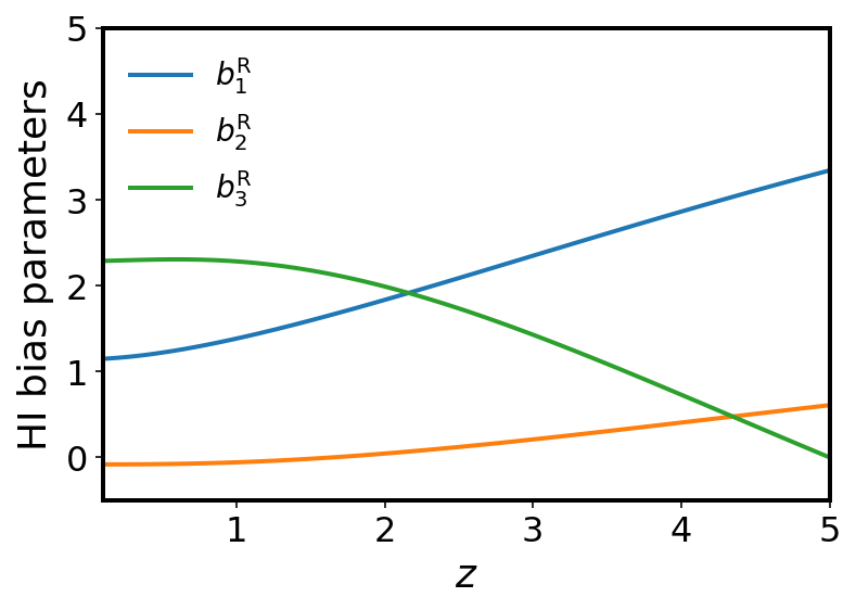
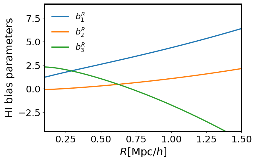
Figure 1: Re-defined HI bias parameters in Equation 3.12 as a function of redshift (left), and re-defined HI bias parameters at $z=1$ as a function of $R$ (right).

The validity of the perturbation theory expansion requires that we restrict attention to scales where the standard deviation is less than unity. For the HI density contrast this implies that $|b^{R}_{1}\sigma_{R}(z)|<1$. On small scales, $R<6\,{\rm Mpc}/h$ at $z=0$, the standard deviation of the dark matter density field is $\sigma_{R}(z)>1$. However, as described in [40], the necessary condition for convergence is that $b_{n+1}^{R}/b_{n}^{R}$ is approximately constant at order $n$. The trade-off is that one needs to go to higher order in perturbation theory to get a converged expression.

One last important feature to note is that $\bar{n}^{R}_{\rm HI}$, $\delta_{\rm HI}^{{R}}$, and $b_{i}^{R}$ are now dependent on the size of the domain containing HI:

$$\frac{\partial\bar{n}^{R}_{\rm HI}(z)}{\partial R}\,,~{}\frac{\partial\delta_{\rm HI}^{R}(z,{\bm{x}})}{\partial R}\,,~{}\frac{\partial b_{i}^{R}(z)}{\partial R}\neq 0\,.$$ (3.13)

This is in agreement with the findings from the analysis of N-body simulations, which shows that these parameters are dependent on the exclusion scale which is determined by the halo mass [12].

3.2 Dependence of HI statistics on splashback radius

We calculate the HI bias parameters defined Equation 3.12 from the model of the local density contrast (halo model) by weighting the halo bias parameters with the HI-halo mass relation:

$$b^{R}_{i}(z)=\frac{1}{{\bar{\rho}}_{\rm HI}(z)}\int_{M_{\rm{min}}(z)}^{\infty}\mathrm{d}M\,b^{i}_{h}(z,M)\,M_{\rm HI}(v_{c0},M)\,n_{h}(z,M)\,,$$ (3.14)

where ${M}$ is the halo mass, $n_{h}$ is the halo mass function, $b^{i}_{h}$ are the $i$th-order halo bias parameters, and ${\bar{\rho}}_{\rm HI}$ is the mean comoving density of HI, defined as the first moment of the HI-halo mass function:

$${\bar{\rho}}_{\rm HI}(z)=\int_{M_{\rm{min}}(z)}^{\infty}\mathrm{d}M\,M_{\rm HI}(v_{c0},M)\,n_{h}(z,M)\,.$$ (3.15)

Here, $M_{\rm{min}}$ is the minimum mass a halo must have in order to host HI.

We need to describe the relationship between the mass enclosed by the comoving sphere of radius $R$, and $M_{{\rm{min}}}$ or $v_{c0}$ introduced in Equation 3.14. We start with the definition of the halo mass introduced in equation Equation 3.14. The halo mass $M$ is defined with respect to a spherical top-hat filter as mass contained within a region of space with density contrast greater than the critical density of the universe by a factor $\Delta_{c}$ [42]

$$M\equiv\frac{4\pi}{3}\bar{\rho}_{\rm{c}}(z)\Delta_{c}(z)R_{c}^{3}(z)={M_{c}}(z)\,,$$ (3.16)

where ${\bar{\rho}}_{c}$ is the critical density of the universe at redshift $z$.

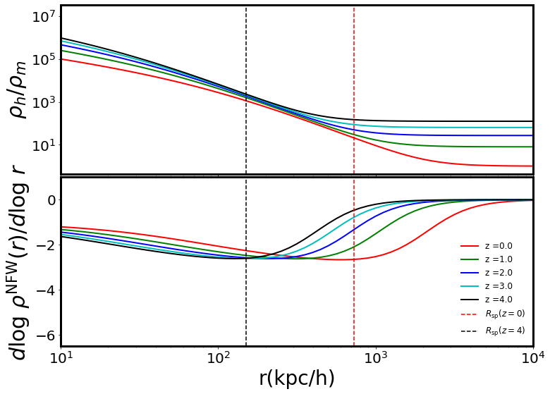
Figure 2: Navarro-Frenk-White halo density profile (top) and its slope (bottom) for a range of redshifts. Splashback radius is shown by vertical lines (black at $z=4$, red at $z=0$).

The radius, $R_{c}$, does not correspond to the physical boundary of the halo because the mass contained within $R_{c}$ is subject to pseudo-evolution (i.e., evolution of the halo mass due to the evolution of the density at the reference redshift [43]), which breaks mass conservation [16]. In addition, recent studies have shown that sub-structures which form during collapse involve processes that redistribute mass from small to large radii greater than $R_{c}$ [44, 45, 46]. For these reasons, in [16] a coordinate-independent definition of the halo boundary was introduced, which includes all matter that orbits the main halo – known as the ‘splashback radius’, $R_{\rm sp}$. It is dynamically defined by particles that reach the apocentre of their first orbit after infall [18, 15]. There is a pile up of particles at the apocentre due to their low radial velocity, thereby creating a caustic that manifests as a sharp drop in the density profile in the halo outskirts , as shown in Figure 2. It has been detected in the Sunyaev-Zel’dovich signal of galaxy clusters [49, 50] and in 3000 optically selected galaxy clusters over a redshift range $0.1<z<1.0$ from the Hyper Suprime-Cam Subaru Strategic Program [51]. Improvements of the theoretical modelling of clustering given the splashback radius are currently being pursued [19, 52, 53, 44, 45, 46] .

To connect $R_{\rm sp}$ to $M_{{\rm{min}}}$, wel use the fitting function given in [16], which specifies the relation between $R_{\rm{sp}}$ and $R_{c}$, then use Equation 3.16 to relate $R_{\rm sp}$ to $M_{{\rm{min}}}$:

$$\frac{R_{\rm{sp}}{(z)}}{R_{c}(z)}=A(z)+B(z)\,{\rm e}^{{\Gamma(z)}/C(z)}\,,$$ (3.17)

where $\Gamma$ is the mass accretion rate and $A$, $B$, $C$ are given in [16] as

$$A(z) =0.54\big{[}1+0.53\,{\Omega_{\rm m}(1+z)^{3}H_{0}^{2}/H^{2}(z)}\big{]}\,,$$ (3.18)

$$B(z) ={1.36\,A(z)\,,}$$ (3.19)

$$C(z) =3.04\,.$$ (3.20)

Although these fitting functions where obtained in [16] at fixed $\Gamma$, subsequent studies have shown that they evolve with redshift [19]. This is most likely due to the physics of mass accretion, which dominates mass growth at very high redshift [54, 55, 56, 57]. Thus, we parametrise $\Gamma$ as $\Gamma(z)=\Gamma_{1}+\Gamma_{2}z$. Using Equation 3.17 and Equation 3.16, we find that $M_{\rm min}$ can be expressed in terms of the splashback radius as

$$M_{\rm{min}}(z|\theta)=\frac{4\pi}{3}\bar{\rho}_{\rm{c}}(z)\Delta_{c}(z)\left[\frac{R_{\rm{sp}}{(z)}}{A(z)+B(z)\,{\rm e}^{-\Gamma/C(z)}}\right]^{3}\,,$$ (3.21)

where $\theta\equiv\left\{R,\Gamma_{1},\Gamma_{2}\right\}$ are physical parameters. Note that $R_{\rm{sp}}$ is a physical (i.e. proper) radius [52]. The corresponding comoving scale is related to $R_{\rm{sp}}$ according to $R_{\rm{sp}}={R/(1+z)}$. We fix the parameter values by comparing our model of the HI density parameter (which represents the comoving density fraction of HI), to the corresponding measurements of $\Omega_{\rm HI}$ made at various redshifts  [58]. Within the halo model, $\Omega_{\rm HI}$ is given by

$$\Omega_{\rm HI}(z|\theta)\equiv\frac{{\bar{\rho}}_{\rm HI}(z|\theta)}{\bar{\rho}_{c0}}\,,$$ (3.22)

where $\bar{\rho}_{c0}=3H^{2}_{0}/8\pi G$. We show the best-fit values in Figure 3. The corresponding mean HI brightness temperature is given by [2].

$$\bar{T}_{\rm HI}(z|\theta)\approx 189h\frac{H_{0}(1+z)^{2}}{H(z)}\Omega_{\rm HI}(z|\theta)\,{\rm mK}\,.$$ (3.23)

With $M_{\rm{min}}$ expressed in terms of $\theta$, the dependence of the HI bias parameters on $R$ is shown in Figure 1.

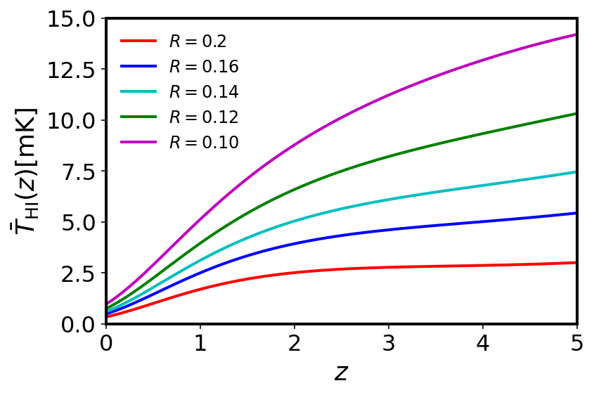
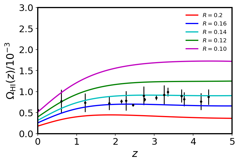
Figure 3: HI brightness temperature Equation 3.23 (left) and $\Omega_{\rm HI}(z)$ dependence on halo size at a fixed accretion rate $\Gamma_{1}=2.3$, $\Gamma_{2}=-0.9$ (right). The dark data points with error bars are observationally determined $\Omega_{\rm HI}(z)$, they were compiled in [47]. $R$ is in Mpc/$h$.

4 HI power spectrum at one-loop and stochasticity

We expand the smoothed HI density contrast given in Equation 3.11 in Fourier space as

$$\delta^{{R}}_{\rm HI}({\bm{k}}) = \mathcal{K}^{(1)}(\bm{k})\delta_{\rm m}({\bm{k}})-\frac{1}{2}b_{2}^{R}\sigma^{2}_{R}{\delta^{(D)}({\bm{k}})}$$

$$+\frac{1}{2}\int\frac{{\rm d}^{3}\bm{k}_{1}}{(2\pi)^{3}}\int\frac{{\rm d}^{3}\bm{k}_{2}}{(2\pi)^{3}}\mathcal{K}^{(2)}({\bm{k}}_{1},{\bm{k}}_{2})\delta_{\rm m}({\bm{k}}_{1})\delta_{\rm m}({\bm{k}}_{2})(2\pi)^{3}\delta^{(D)}\left({\bm{k}}-{\bm{k}}_{1}-{\bm{k}}_{2}\right)$$

$$+\frac{1}{3!}\int\frac{{\rm d}^{3}\bm{k}_{1}}{(2\pi)^{3}}\int\frac{{\rm d}^{3}\bm{k}_{2}}{(2\pi)^{3}}\int\frac{{\rm d}^{3}\bm{k}_{3}}{(2\pi)^{3}}\mathcal{K}^{(3)}({\bm{k}}_{1},{\bm{k}}_{2},{\bm{k}}_{3})\delta_{\rm m}({\bm{k}}_{1})\delta_{\rm m}({\bm{k}}_{2})\delta_{\rm m}({\bm{k}}_{3})$$

$$\times(2\pi)^{3}\delta^{(D)}\left({\bm{k}}-{\bm{k}}_{1}-{\bm{k}}_{2}-{\bm{k}}_{3}\right)\,,$$

where we have introduced the following Fourier space kernels

$$\mathcal{K}^{(1)}({\bm{k}}) =b^{R}_{1}W_{R}({k})\,,$$ (4.2)

$$\mathcal{K}^{(2)}({\bm{k}}_{1},{\bm{k}}_{2}) =W_{R}({k}_{1})W_{R}({k}_{2})b_{2}^{R}+W_{R}({k})b_{1}^{R}F_{2}({\bm{k}}_{1},{\bm{k}}_{2})\,,$$ (4.3)

$$\mathcal{K}^{(3)}({\bm{k}}_{1},{\bm{k}}_{2},{\bm{k}}_{3}) =W_{R}({k}_{1})W_{R}({k}_{2})W_{R}({k}_{3})b_{3}^{R}+b_{1}^{R}W_{R}({k})F_{3}({\bm{k}}_{1},{\bm{k}}_{2},{\bm{k}}_{3})$$ (4.4)

$$+{b_{2}^{R}\left[W_{R}({k}_{3})W_{R}({|{\bm{k}}_{1}+{\bm{k}}_{2}|})F_{2}({\bm{k}}_{1},{\bm{k}}_{2})+2W_{R}({k}_{1})W_{R}({|{\bm{k}}_{2}+{\bm{k}}_{3}|})F_{2}({\bm{k}}_{2},{\bm{k}}_{3})\right]}\,.$$

Here, we made use of the Fourier space kernels for the dark matter density field in an Einstein de Sitter universe [59]

$${F}_{2}({\bm{k}}_{1},{\bm{k}}_{2})={10\over 7}+{{\bm{k}}_{1}\cdot{\bm{k}}_{2}\over k_{1}k_{2}}\left({k_{1}\over k_{2}}+{k_{2}\over k_{1}}\right)+{4\over 7}\left({{\bm{k}}_{1}\cdot{\bm{k}}_{2}\over k_{1}k_{2}}\right)^{2},$$ (4.5)

and $F_{3}$ is given in [60]. These kernels are valid as well in the $\Lambda$CDM universe provided that the $\Lambda$CDM cosmological parameters are used to evaluate the power spectrum [61, 62]. We find that the auto-power spectrum of the HI density contrast is given by

$${P}_{\rm HI}^{(c)}({k},R) ={P}_{\rm HI}^{11}({k},R)+{P}_{\rm HI}^{22}({k},R)+{P}_{\rm HI}^{13}({k},R)\,,$$

$$=\left[\mathcal{K}^{(1)}({k})\right]^{2}P^{11}_{\rm m}(k)+\frac{1}{2}\int\frac{{\rm d}^{3}\bm{k}_{1}}{(2\pi)^{3}}\left[\mathcal{K}^{(2)}({\bm{k}}_{1},|{\bm{k}}-{\bm{k}}_{1}|)\right]^{2}P^{11}_{\rm m}({k}_{1})P^{11}_{\rm m}(|{\bm{k}}-{\bm{k}}_{1}|)$$

$$\phantom{=}+\frac{1}{3}\mathcal{K}^{(1)}({k})P^{11}_{\rm m}(k)\int\frac{{\rm d}^{3}\bm{k}_{1}}{(2\pi)^{3}}\mathcal{K}^{(3)}({\bm{k}}_{1},-{\bm{k}}_{1},{k})P^{11}_{\rm m}({k}_{1})\,,$$ (4.6)

where ${P}_{\rm HI}^{11}$ is the linear HI power spectrum, $P^{11}_{\rm m}$ is the linear matter power spectrum and ${P}_{\rm HI}^{22}({k})+{P}_{\rm HI}^{13}({k})$ constitutes the one-loop correction. In the long-wavelength limit, $F_{2}$ in $P_{\rm HI}^{22}$ vanishes. However, the non-linear bias term $b_{2}^{R}$ term (first term in Equation 4.3) does not vanish.

$$P_{\rm HI}^{22}(k,R)~{}~{}\xrightarrow{k\to 0}~{}~{}\frac{1}{2}\left(b^{R}_{2}\right)^{2}\int\frac{{\rm d}^{3}\bm{k}_{1}}{(2\pi)^{3}}W_{R}^{4}({k}_{1})\big{(}{P_{\rm m}^{11}}\big{)}^{2}({k}_{1})\equiv N_{\rm eff}{(R)}\,.$$ (4.7)

Here, $N_{\rm eff}$, denotes the non-vanishing part of $P_{\rm HI}^{22}$ in the limit of zero momentum. This term is referred to as induced stochasticity [11], as white noise [23], or as the contact term [25]. It is not clear whether this term has an observational consequence [20, 21, 22] and we revisit this issue in subsection 4.1. Before we proceed, we note that the same non-linear bias parameter responsible for the re-definition of the one-point statistics in Equation 3.10 is also responsible for the emergent white noise-like feature at the two-point correlation function level on large scales.

It is possible to analytically simplify the terms in the last line of Equation 4.6 as

$$P_{\rm HI}^{13}(k,R)=W^{2}_{R}({k})\left\{\frac{1}{2}\left[b^{R}_{1}b^{R}_{3}\sigma^{2}_{R}+b^{R}_{1}b^{R}_{2}\sigma^{2}_{b^{R}_{1}b_{2}^{R}}(k,R)\right]P_{\rm m}^{11}(k)+{(b^{R}_{1})}^{2}P^{13}_{\rm m}(k)\right\}\,,$$ (4.8)

where $\sigma^{2}_{b^{R}_{1}b_{2}^{R}}$ is defined below. $P^{13}_{\rm m}$ is the matter power spectrum equivalent of $P_{\rm HI}^{13}$, the full expression is given in [63]. $P^{13}_{\rm HI}$ is ultraviolet sensitive, in effective field theory of large scale structure a counter-term is usually added to remove the divergence [64, 65, 66]. Here, the problem is parametrically controlled by the window function, thereby eliminating the need to run an N-body simulation to calibrate the counter-term. Putting all this together leads to

$$P_{\rm{\rm HI}}^{(c)}(k,R)=W^{2}_{R}({k})\left[(b^{R}_{1})^{2}P_{\rm m}(k)+\frac{1}{2}\left(b^{R}_{1}b^{R}_{3}\sigma^{2}_{R}+b^{R}_{1}b^{R}_{2}\sigma^{2}_{b^{R}_{1}b_{2}^{R}}(k,R)\right)P^{11}_{\rm m}(k)\right]\\ +{b^{R}_{1}b^{R}_{2}}P_{b^{R}_{1}b_{2}^{R}}(k,R)+{\left(b^{R}_{2}\right)^{2}}P_{b^{R}_{2}b_{2}^{R}}(k,R)+N_{\rm eff}{(R)}\,,$$ (4.9)

where $P_{\rm m}(k)$ is the matter power spectrum up to one-loop order and

$$P_{b^{R}_{1}b_{2}^{R}}(k,R) =\frac{1}{2}\int\frac{{\rm d}^{3}\bm{k}_{1}}{(2\pi)^{3}}\bigg{[}W_{R}({k})W_{R}({k}_{1})W_{R}({k}_{2})F_{2}({\bm{k}}_{1},{\bm{k}}_{2})\bigg{]}P^{11}_{\rm m}({k}_{2})P^{11}_{\rm m}(k_{1})\,,$$ (4.10)

$$P_{b^{R}_{2}b_{2}^{R}}(k,R) =\frac{1}{2}\int\frac{{\rm d}^{3}\bm{k}_{1}}{(2\pi)^{3}}\bigg{[}W^{2}_{R}({k}_{1})W^{2}_{R}({k}_{2})P^{11}_{\rm m}({k}_{2})P^{11}_{\rm m}(k_{1})-W_{R}^{4}({k}_{1})\big{\{}{P_{\rm m}^{11}}({k}_{1})\big{\}}^{2}\bigg{]}\,,$$ (4.11)

$$\sigma_{b^{R}_{1}b_{2}^{R}}(k,R) =2\int\frac{{\rm d}^{3}\bm{k}_{1}}{(2\pi)^{3}}\bigg{[}\frac{W_{R}({k}_{1})W_{R}({|\bm{k}_{1}-\bm{k}|})}{W_{R}({k})}F_{2}(-{\bm{k}}_{1},{\bm{k}})\bigg{]}P^{11}_{\rm m}({k}_{1})\,.$$ (4.12)

Essentially, we have decomposed $P_{\rm HI}^{22}$ term that appear in Equation 4.6 into scale dependent part (Equation 4.11) and scale independent part (Equation 4.7). In evaluating the integrals, we defined $\mu_{k}={\bm{k}}_{1}\cdot{\bm{k}}/kk_{1}$, and use momentum conservation ${\bm{k}}_{2}={\bm{k}}-{\bm{k}}_{1}$, to set $k_{2}=k\sqrt{r^{2}-2r\mu_{k}-1}=ky$, where $k_{1}=kr$, $y=\sqrt{r^{2}-2r\mu_{k}+1}$. The $k$-integrals in Equation 4.10 to Equation 4.12 can be performed optimally using the FFTLog formalism [67, 68].

Finally, the HI power spectrum in the continuous limit(Equation 4.9) may be decomposed into two terms,

$$P_{\rm{\rm HI}}^{(c)}(k,R)=P_{\rm{\rm HI}}^{(s)}(k,R)+N_{\rm eff}{(R)}\,,$$ (4.13)

where $P_{\rm{\rm HI}}^{(s)}$ is the HI power spectrum without the emergent non-linear white noise term $N_{\rm eff}$:

$$P_{\rm{\rm HI}}^{(s)}(k,R)=W^{2}_{R}({k})(b^{R}_{1})^{2}P_{\rm m}(k)+\frac{1}{2}\left[b^{R}_{1}b^{R}_{3}\sigma^{2}_{R}+b^{R}_{1}b^{R}_{2}\sigma^{2}_{b^{R}_{1}b_{2}^{R}}(k,R)\right]P^{11}_{\rm m}(k)\\ \ +{b^{R}_{1}b^{R}_{2}}P_{b^{R}_{1}b_{2}^{R}}(k,R)+{\left(b^{R}_{2}\right)^{2}}P_{b^{R}_{2}b_{2}^{R}}(k,R)\,.$$ (4.14)

We made use of the halo-fit in CAMB to compute $P_{\rm m}$ [69], and the standard linear order Einstein-Boltzmann result from CAMB to compute $P^{11}_{\rm m}$ [70] . The results are shown in Figure 4.

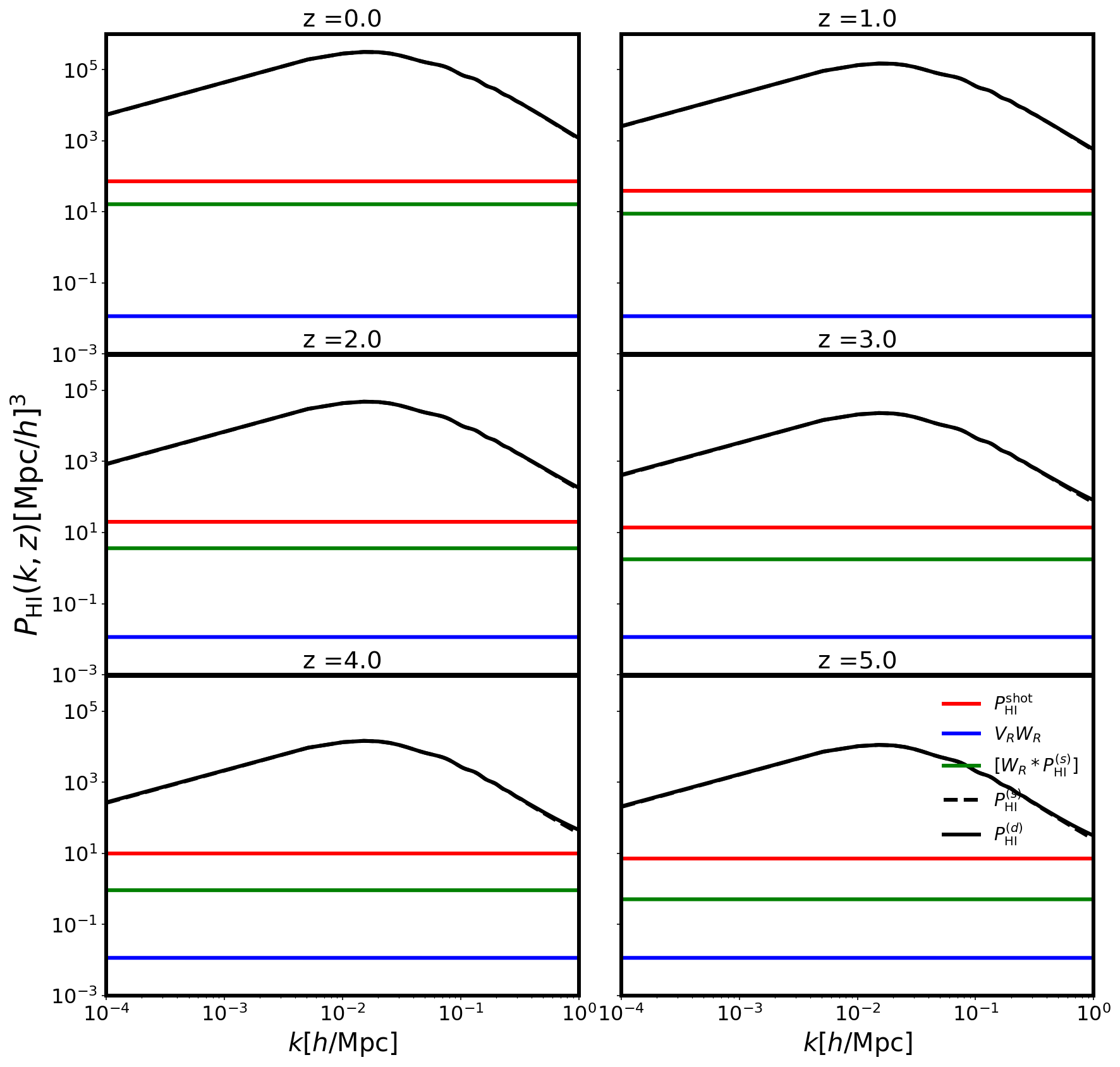
Figure 4: HI power spectrum at different redshifts at the best-fitting $R$, ${\Gamma_{1}}$ and ${\Gamma_{2}}$. The $k_{1}$-integral in subsection 4.1 is UV sensitive, hence, we set $k_{\rm{max}}=1/R$ for simplicity.

4.1 Finite size resolves emergent large-scale white noise problem

Here we show that $N_{\rm eff}$ is exactly cancelled in the full expression of the discrete HI power spectrum when the size of haloes is taken into consideration.

Substituting Equation 4.13 in Equation 2.21 leads to

$$P^{(d)}_{\rm HI}(k)=P_{\rm HI}^{\text{shot}}+N_{\rm eff}(R)-V_{{R}}W_{R}(k)-\big{[}{W_{R}}\star P_{\rm HI}^{(c)}\big{]}(k)+P_{\rm{\rm HI}}^{(s)}(k)\,.$$ (4.15)

To appreciate the full structure of Equation 4.15, we have to simplify the convolution term ${W_{R}}\star P_{\rm HI}^{(c)}$ further. Using Equation 2.11 and Equation 4.13, with $\bm{x}\equiv\bm{x}_{12}$, we obtain

$$\big{[}{W_{R}}\star P_{\rm HI}^{(c)}\big{]}({k}) =\int_{{x<R}}{\rm d}^{3}\bm{x}\,\xi_{\rm HI}^{(c)}({x})\,{\rm e}^{-i{\bm{k}}\cdot{\bm{x}}}={\int_{{x<R}}{\rm d}^{3}\bm{x}\big{[}\xi_{\rm HI}^{(s)}({x})+N_{\rm{eff}}\,\delta^{{(\rm D)}}({\bm{x}})\big{]}{\rm e}^{-i{\bm{k}}\cdot{\bm{x}}}}\,,$$

$$={\int}\frac{{\rm d}^{3}\bm{k}_{1}}{(2\pi)^{3}}\,P^{(s)}_{\rm HI}({k}_{1})\,\int_{{x<R}}{\rm d}^{3}\bm{x}\,{\rm e}^{i(\bm{k}_{1}-{\bm{k}})\cdot{\bm{x}}}+{N_{\rm eff}}\int_{{x<R}}{\rm d}^{3}\bm{x}\,\delta^{{(\rm D)}}({\bm{x}})\,{\rm e}^{-i{\bm{k}}\cdot{\bm{x}}}\,,$$

$$=2V_{R}\int_{0}^{\infty}\frac{{\rm d}k_{1}}{\pi}\,k_{1}^{2}\,P^{(s)}_{\rm HI}({k}_{1})\,{\cal W}_{R}(k_{1},k)+{\rm{sgn}}(R)\,{N_{\rm eff}}(R)\,.$$ (4.16)

In the last line, we used Equation 2.17 to obtain the first term.

$$\int\frac{{\rm d}^{3}\bm{k}_{1}}{(2\pi)^{3}}\,P^{(s)}_{\rm HI}({k}_{1})\int_{{x<R}}{\rm d}^{3}\bm{x}\,{\rm e}^{i(\bm{k}_{1}-{\bm{k}})\cdot{\bm{x}}} = \int_{x<R}\frac{{\rm d}^{3}\bm{x}}{(2\pi)^{2}}\,{\rm e}^{-i{\bm{k}}\cdot{\bm{x}}}\int_{0}^{\infty}{\rm d}k_{1}\,k_{1}^{2}\,P^{(s)}_{\rm HI}({k}_{1})\int_{-1}^{1}{\rm d}\mu_{1}\,{\rm e}^{i{k_{1}}x\mu_{1}}$$ (4.17)

$$= 2V_{R}\int_{0}^{\infty}\frac{{\rm d}k_{1}}{\pi}\,k_{1}^{2}\,P^{(s)}_{\rm HI}({k}_{1})\,{\cal W}_{R}(k_{1},k)\,,$$

where

$${\cal W}_{R}(k_{1},k)=\begin{cases}{k\left[(k_{1}/k)\cos(k_{1}R)\sin(kR)-\cos(kR)\sin(k_{1}R)\right]\over(kR)^{3}k_{1}(1-k_{1}^{2}/k^{2})}~{}~{}~{}~{}\qquad{\rm{for}}~{}k\neq k_{1}\,,\\ \\ {{\left[2kR-\sin(2kR)\right]}\over 4(kR)^{3}}\hskip 142.26378pt{\rm{for}}~{}k=k_{1}\,.\\ \end{cases}$$ (4.18)

For the second term, we expand the delta function in spherical coordinates and perform the resulting integral analytically

$$\int_{{x<R}}{\rm d}^{3}x_{12}\delta^{({\rm D})}({\bm{x}})e^{-i{\bm{k}}\cdot{\bm{x}}}=\int_{0}^{R}{{\rm d}}r\delta^{{(\rm D})}({r})j_{0}(kr)={\rm{sgn}}(R)\,,$$ (4.19)

where ${\rm{sgn}}(R)$ is a sigmoid function and for $R\geq 0$, it is given by

$${\rm{sgn}}(R):=\begin{cases}0&\text{if }R=0\\ 1&\text{if }R>0.\end{cases}$$ (4.20)

Putting Equation 4.16 back into Equation 4.15 we obtain the final result:

$$P^{(d)}_{\rm HI}(k,R) = P_{{\rm HI}}^{(s)}(k,R)+P_{\rm HI}^{\text{shot}}+N_{\rm eff}(R)\left[1-{\rm{sgn}}(R)\right]$$

$$\qquad\qquad-V_{{R}}W_{R}(k)-2V_{R}\int_{0}^{\infty}\frac{{\rm d}k_{1}}{\pi}\,k_{1}^{2}\,P^{(s)}_{\rm HI}({k}_{1})\,{\cal W}_{R}(k_{1},k)\,.$$

subsection 4.1 shows that for $R>0$, i.e. if the finite size of haloes is taken into account, then the $N_{\rm eff}$ term drops out exactly. By contrast, in the peak approximation, i.e. the limit where $R\to 0$ and $V_{R}\to 0$, the $N_{\rm eff}$ term does not drop out, so we recover the standard result [23, 24, 25, 20, 21, 22]

$$P^{(d)}_{\rm HI}(k)=P_{\rm{\rm HI}}^{(s)}(k)+P_{\rm HI}^{\text{shot}}+N_{\rm eff}\,.$$ (4.22)

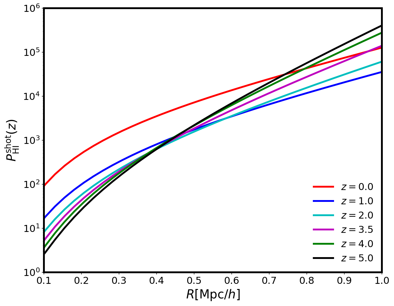
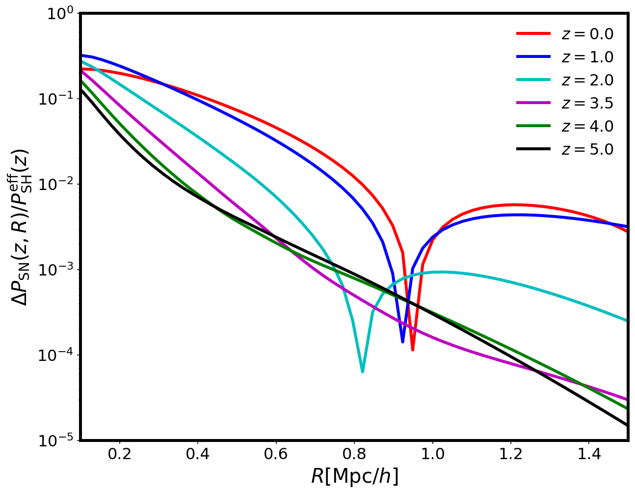
Figure 5: HI shot noise at the best-fit value of accretion rate(left). Difference between effective shot noise and intrinsic shot noise at the best-fit value of accretion rate(right). For the effective shot noise we set $k=0.001$ h/Mpc.

subsection 4.1 is an important result. We have shown, for the first time, that the emergent large-scale white noise is as a result of the breakdown of the peak approximation for the tracer density field. This provides more clarity on how to handle $N_{\rm eff}$ in standard perturbation theory or in effective field theory approaches – avoiding the need to set $N_{\rm eff}$ to zero [25] by hand or absorbing it into the shot noise [23, 24] which does not work for the HI brightness temperature [20, 21, 22] since the halo model predicts shot noise with smaller amplitude when compared to the amplitude of $N_{\rm eff}$. We have now shown that this term vanishes exactly as soon as the finite size of the source is taken into account.

Comparing subsection 4.1 to Equation 2.13, the second and third terms can be re-written as part of the effective shot noise contribution

$$P^{\rm{eff}}_{\rm{SN}}(k,R) =P_{\rm HI}^{\text{shot}}-V_{{R}}W_{R}(k)-2V_{R}\int_{0}^{\infty}\frac{{\rm d}k_{1}}{\pi}\,k_{1}^{2}\,P^{(s)}_{\rm HI}({k}_{1})\,{\cal W}_{R}(k_{1},k)\,,$$ (4.23)

$$\approx P_{\rm HI}^{\text{shot}}\qquad{\rm{for}}\qquad R<1~{}{\rm{Mpc}/h}\,,$$ (4.24)

where the Poisson shot noise, $P_{\rm HI}^{\text{shot}},$ is obtained by weighting the halo density field appropriately with the HI-halo mass relation [1, 5], namely

$$P_{\rm HI}^{\text{shot}}(R)=\frac{1}{\bar{n}^{R}_{\rm{HI}}}=\frac{1}{{\bar{\rho}}^{2}_{\rm HI}(z)}\int_{M_{\rm{min}}}^{\infty}{\rm d}M\,M_{\rm HI}^{2}(M)\,n_{h}(z,M)\,.$$ (4.25)

For $R\ll 1\,{\rm Mpc}/h$, the second term and the third term are negligible, see Figure 5. For massive halos, i.e $R\geq 1\,{\rm Mpc}/h$, one would expect the amplitude of the effective shot noise term to be substantially modulated by the size of the excluded region, as inthe right panel of Figure 5. In the right panel of Figure 5, we plot the fractional difference between the effective shot noise and the intrinsic shot noise: $\Delta P_{\rm{SN}}(k,R)=P^{\rm{eff}}_{\rm{SN}}(k,R)-P_{\rm HI}^{\text{shot}}$. This shows that for HI with $R>0.14\,{\rm Mpc}/h$, the effect of the sub-Poissonian noise correction peaks at the comoving boundary of the halo containing HI, it decreases away from the halo boundary. We find that increasing $R$ while keeping every other parameter fixed for the HI, the contribution from the last term in subsection 4.1 changes sign at $R$ away from the comoving halo boundary.

5 Summary and Outlook

5.1 Consequences of the exclusion region

The standard halo model framework and its various extensions [71, 72] split the mass distribution in the Universe into distinct regions. The correlation function is split into correlations between the distinct regions and correlations within each region. These are the well-known one- and two-halo terms for the two-point correlation function. Standard perturbation theory, on the other hand, does not make this distinction, it assumes that the perturbation theory expansion is valid at all locations, even within highly dense dark matter haloes. This assumption leads to the well-known ultraviolet problems at the loop level and non-linear white noise in the infra-red due to contact terms [25].

We have argued that the physics of clustering imposes a physical scale which is related to the dynamically defined splashback radius of haloes that allow treatment of structure evolution in line with the halo model. There are few key points to highlight:

• Significance of the splashback radius: We have proposed a connection between the minimum halo mass that can host HI and the physical halo boundary. This connection involves the mass accretion rate, which impacts, the growth of the physical halo boundary. The accretion rate and halo boundary are physical parameters that future surveys such as HI intensity mapping with HIRAX [73], MeerKAT [74], SKA [2] and others could provide an opportunity to constrain.

• Cancellation of the induced white noise: Any tracer power spectrum at one-loop within the standard perturbation theory has a component which does not vanish in the limit of zero momentum. This behaviour is also present in the standard halo model of the matter power spectrum, in this case, the one-halo term leads to a non-zero contribution in the limit of zero momentum [75]. The non-vanishing component is referred to as induced stochasticity in [11], as white noise in [23], or as the contact term that leads to a delta function in real space in [25]. It was observed in [20, 21, 22] that it could have consequences for the bias parameters on large scales for the HI brightness temperature if indeed it is physical. We have shown that this term vanishes exactly as soon as the size of the discrete source is taken into account.

• Mass weighting of haloes: We have shown that it is possible to minimise $P^{\rm{eff}}_{\rm{SN}}(k,R)$ by taking the finite halo size into consideration. Setting $R$ to its corresponding physical boundary value gives the minimum effective shot noise (see Figure 5). A similar idea has been explored in estimating the halo power spectrum from the N-body simulations but in that context, it is known as mass weighting of haloes [26]. The connection between mass weighting of haloes and halo exclusion criteria was made in [11]. Essentially, choosing different mass bins(mass weighting) corresponds to choosing the most optimal $R$ that minimaxes $P^{\rm{eff}}_{\rm{SN}}(k,R)$ the most. This idea was used in [76, 77] to show how shot noise associated with the halo power spectrum could be significantly suppressed on large scales thereby improving the signal to noise ratio.

• Sub-Poissonian process: We have shown that the noise associated with discrete tracers is not entirely due to a Poisson process, i.e. $P^{\rm{eff}}_{\rm{SN}}(k,R)\neq 1/\bar{n}_{\rm HI}$, there would be a sub-Poissonian contribution. This feature has already been observed both in cluster auto-and cluster-galaxy cross-correlations of the Sloan Digital Sky Survey [78].

5.2 Conclusions

Our understanding of the universe through large scale structure has relied heavily on the halo model [4]. Haloes in this context are not point sources, but rather virialized extended objects with finite boundaries given by the splashback radius [15]. Luminous objects such as galaxies and neutral hydrogen are situated inside haloes and held together by the self-gravitational field of haloes [13]. However for the halo power spectrum in standard perturbation theory, haloes are modelled as point sources on all scales [79]. We have shown how to take into account the physical constraints due to the finite size of the halo in modelling the power spectrum of the HI brightness temperature.

The standard practice is to model tracers as point sources, in this limit the power spectrum is given as a sum of the continuous power spectrum and the Poisson shot noise (see Equation 2.13). The Poisson shot noise is given by the mean number density of the tracer. In addition to the Poisson shot noise, there is also a non-linear white noise contribution from the continuous power spectrum in the limit of zero momentum. This suggests a break down of the mass-energy conservation for tracers [75]. We have shown that taking into account the finite size of haloes introduces two additional terms to the power spectrum of discrete tracers (see Equation 2.21). The two extra terms describe the fact that information with wavelength less than the size of haloes is uncorrelated and therefore defines the exclusion region. We have shown that taking the exclusion region into account leads to an exact cancellation of the non-linear white noise-like term that appears in the limit of zero momentum (see subsection 4.1). We showed that the effective shot noise contribution on large scales is sub-Poissonian and it is dependent on the size of the exclusion region.

For the HI brightness temperature, we argued that the exclusion region is naturally given by the splashback radius of the halo with the minimum mass required to host HI. We describe how the HI brightness temperature within haloes of a given mass or size may be modelled as a tracer of the dark matter density field. Finally, we argued that taking into account the consequences of the finite size of haloes in modelling the power spectrum of any tracer may explain why the concept of mass-weighting of haloes improves the signal-to-noise ratio [76, 77].

Appendix A Basic tools of the halo model

We calculate the bias parameters from the Sheth-Tormen halo mass function for a spherical collapse model [42]:

$$n_{h}(M)=\nu f(\nu)\frac{\bar{\rho}}{M^{2}}\frac{{\rm d}\ln\nu}{{\rm d}\ln M},$$ (A.1)

where the peak height $\nu$ is related to the variance in dark matter density field, $\sigma^{2}_{\rm m}$, $\nu=(\delta_{c}/\sigma_{\rm m})^{2}$ and $\delta_{c}=1.686$ is the critical threshold for a spherical collapse at the current epoch obtained from linear perturbation theory. A halo of mass $M=\bar{\rho}V$ is formed when the walk first crosses a barrier $f(\nu)$:

$$\nu f(\nu)=A(p)\left(1+\frac{1}{(q\nu)^{p}}\right)\sqrt{\frac{q\nu}{2\pi}}\exp\left(-\frac{q\nu}{2}\right),$$ (A.2)

where $q=0.707$ and $p=0.3$ are obtained from a fit to numerical simulations. The halo bias parameters up to third order are given by [4]

$$b^{h}_{1} =1+\frac{(q\nu-1)}{\delta_{c}}+\frac{2p}{\delta_{c}\left(1+(q\nu)^{p}\right)}\,,$$ (A.3)

$$b^{h}_{2} =\frac{8}{21}\left(b_{1}-1\right)+\frac{4\left(p^{2}+\nu pq\right)-(q\nu-1)\left(1+(q\nu)^{p}\right)-2p}{\delta^{2}_{c}\left(1+(q\nu)^{p}\right)}+\frac{1}{\delta_{c}^{2}}\left((q\nu)^{2}-2q\nu-1\right)\,$$ (A.4)

$$b^{h}_{3} =-\frac{236}{189}\left(b_{1}-1\right)-\frac{13}{7}\left(b_{2}-\frac{8}{21}\left(b_{1}-1\right)\right)-\frac{\left(3+3\nu q+3\nu^{2}q^{2}-\nu^{3}q^{3}\right)}{\delta_{c}^{3}}$$ (A.5)

$$+\frac{\left(8p^{3}+12p^{2}\left(1+\nu q\right)+p\left(6\nu^{2}q^{2}-2\right)\right)}{\delta_{c}^{3}\left(1+1+(\nu q)^{p}\right)}+6\frac{\left(1+2\nu q-\nu^{2}q^{2}\right)}{\delta_{c}^{3}}-24\frac{\left(p^{2}+\nu pq\right)}{\delta_{c}^{3}\left(1+(\nu q)^{p}\right)}$$

$$-4\frac{(1-\nu q)}{\delta_{c}^{3}}+8\frac{p}{\delta_{c}^{3}\left(1+(q\nu)^{p}\right)}\,,$$

References

- [1] P. Bull, P. G. Ferreira, P. Patel, and M. G. Santos, Late-time cosmology with 21cm intensity mapping experiments, arXiv:1405.1452.
- [2] M. G. Santos et al., Cosmology with a SKA HI intensity mapping survey, arXiv:1501.03989.
- [3] J. F. Navarro, C. S. Frenk, and S. D. M. White, The Structure of cold dark matter halos, Astrophys. J. 462 (1996) 563–575, [astro-ph/9508025].
- [4] A. Cooray and R. K. Sheth, Halo Models of Large Scale Structure, Phys. Rept. 372 (2002) 1–129, [astro-ph/0206508].
- [5] H. Padmanabhan, A. Refregier, and A. Amara, A halo model for cosmological neutral hydrogen : abundances and clustering H i abundances and clustering, Mon. Not. Roy. Astron. Soc. 469 (2017), no. 2 2323–2334, [arXiv:1611.06235].
- [6] M. J. Rees, Lyman absorption lines in quasar spectra - Evidence for gravitationally-confined gas in dark minihaloes, MNRAS 218 (Jan., 1986) 25P–30P.
- [7] G. Efstathiou, Suppressing the formation of dwarf galaxies via photoionization, MNRAS 256 (May, 1992) 43P–47P.
- [8] R. Casas-Miranda, H. Mo, R. K. Sheth, and G. Boerner, On the Distribution of Haloes, Galaxies and Mass, Mon. Not. Roy. Astron. Soc. 333 (2002) 730–738, [astro-ph/0105008].
- [9] R. K. Sheth and G. Tormen, An Excursion set model of hierarchical clustering : Ellipsoidal collapse and the moving barrier, Mon. Not. Roy. Astron. Soc. 329 (2002) 61, [astro-ph/0105113].
- [10] F. van den Bosch, S. More, M. Cacciato, H. Mo, and X. Yang, Cosmological Constraints from a Combination of Galaxy Clustering and Lensing – I. Theoretical Framework, Mon. Not. Roy. Astron. Soc. 430 (2013), no. 2 725–746, [arXiv:1206.6890].
- [11] T. Baldauf, U. s. Seljak, R. E. Smith, N. Hamaus, and V. Desjacques, Halo stochasticity from exclusion and nonlinear clustering, Phys. Rev. D 88 (2013), no. 8 083507, [arXiv:1305.2917].
- [12] R. Garcia and E. Rozo, Halo Exclusion Criteria Impacts Halo Statistics, Mon. Not. Roy. Astron. Soc. 489 (2019), no. 3 4170–4175, [arXiv:1903.01709].
- [13] R. K. Sheth and G. Lemson, Biasing and the distribution of dark matter haloes, Mon. Not. Roy. Astron. Soc. 304 (1999) 767, [astro-ph/9808138].
- [14] R. Garcia, E. Rozo, M. R. Becker, and S. More, A Redefinition of the Halo Boundary Leads to a Simple yet Accurate Halo Model of Large Scale Structure, arXiv:2006.12751.
- [15] S. Adhikari, N. Dalal, and R. T. Chamberlain, Splashback in accreting dark matter halos, JCAP 11 (2014) 019, [arXiv:1409.4482].
- [16] S. More, B. Diemer, and A. Kravtsov, The splashback radius as a physical halo boundary and the growth of halo mass, Astrophys. J. 810 (2015), no. 1 36, [arXiv:1504.05591].
- [17] N. Banik, G. Bertone, J. Bovy, and N. Bozorgnia, Probing the nature of dark matter particles with stellar streams, JCAP 07 (2018) 061, [arXiv:1804.04384].
- [18] B. Diemer and A. V. Kravtsov, Dependence of the outer density profiles of halos on their mass accretion rate, Astrophys. J. 789 (2014) 1, [arXiv:1401.1216].
- [19] B. Diemer, P. Mansfield, A. V. Kravtsov, and S. More, The splashback radius of halos from particle dynamics. II. Dependence on mass, accretion rate, redshift, and cosmology, Astrophys. J. 843 (2017), no. 2 140, [arXiv:1703.09716].
- [20] O. Umeh, R. Maartens, and M. Santos, Nonlinear modulation of the HI power spectrum on ultra-large scales. I, JCAP 1603 (2016), no. 03 061, [arXiv:1509.03786].
- [21] O. Umeh, Imprint of non-linear effects on HI intensity mapping on large scales, JCAP 1706 (2017), no. 06 005, [arXiv:1611.04963].
- [22] A. Pénin, O. Umeh, and M. Santos, A scale dependent bias on linear scales: the case for HI intensity mapping at z=1, Mon. Not. Roy. Astron. Soc. 473 (2018), no. 4 4297–4305, [arXiv:1706.08763].
- [23] P. McDonald, Clustering of dark matter tracers: Renormalizing the bias parameters, Phys.Rev. D74 (2006) 103512, [astro-ph/0609413].
- [24] P. McDonald and A. Roy, Clustering of dark matter tracers: generalizing bias for the coming era of precision LSS, JCAP 0908 (2009) 020, [arXiv:0902.0991].
- [25] V. Assassi, D. Baumann, D. Green, and M. Zaldarriaga, Renormalized Halo Bias, JCAP 1408 (2014) 056, [arXiv:1402.5916].
- [26] U. Seljak, N. Hamaus, and V. Desjacques, How to suppress the shot noise in galaxy surveys, Phys. Rev. Lett. 103 (2009) 091303, [arXiv:0904.2963].
- [27] Planck Collaboration, N. Aghanim et al., Planck 2018 results. VI. Cosmological parameters, Astron. Astrophys. 641 (2020) A6, [arXiv:1807.06209].
- [28] J. Carretero, F. Castander, E. Gaztanaga, M. Crocce, and P. Fosalba, An algorithm to build mock galaxy catalogues using MICE simulations, Mon. Not. Roy. Astron. Soc. 447 (2015) 650, [arXiv:1411.3286].
- [29] H. Padmanabhan, A. Refregier, and A. Amara, Impact of astrophysics on cosmology forecasts for 21 cm surveys, Mon. Not. Roy. Astron. Soc. 485 (2019), no. 3 4060–4070, [arXiv:1804.10627].
- [30] C. Pitrou, A. Coc, J.-P. Uzan, and E. Vangioni, Deuterium: a new bone of contention for cosmology?, arXiv:2011.11320.
- [31] S. Camera and H. Padmanabhan, Beyond CDM with H i intensity mapping: robustness of cosmological constraints in the presence of astrophysics, Mon. Not. Roy. Astron. Soc. 496 (2020), no. 4 4115–4126, [arXiv:1910.00022].
- [32] G. L. Bryan and M. L. Norman, Statistical Properties of X-Ray Clusters: Analytic and Numerical Comparisons, ApJ 495 (Mar., 1998) 80–99, [astro-ph/9710107].
- [33] J. M. Bardeen, J. R. Bond, N. Kaiser, and A. S. Szalay, The Statistics of Peaks of Gaussian Random Fields, Astrophys. J. 304 (1986) 15–61.
- [34] P. J. E. Peebles and E. J. Groth, An integral constraint for the evolution of the galaxy two-point correlation function., A&A 53 (Nov., 1976) 131–140.
- [35] A. Hall, C. Bonvin, and A. Challinor, Testing General Relativity with 21-cm intensity mapping, Phys. Rev. D87 (2013), no. 6 064026, [arXiv:1212.0728].
- [36] S. Seehars, A. Paranjape, A. Witzemann, A. Refregier, A. Amara, and J. Akeret, Simulating the Large-Scale Structure of HI Intensity Maps, JCAP 03 (2016) 001, [arXiv:1509.01589].
- [37] F. Villaescusa-Navarro et al., Ingredients for 21 cm Intensity Mapping, Astrophys. J. 866 (2018), no. 2 135, [arXiv:1804.09180].
- [38] V. Desjacques, D. Jeong, and F. Schmidt, Large-Scale Galaxy Bias, Phys. Rept. 733 (2018) 1–193, [arXiv:1611.09787].
- [39] D. Wadekar, F. Villaescusa-Navarro, S. Ho, and L. Perreault-Levasseur, Modeling assembly bias with machine learning and symbolic regression, arXiv:2012.00111.
- [40] F. Schmidt, D. Jeong, and V. Desjacques, Peak-Background Split, Renormalization, and Galaxy Clustering, Phys. Rev. D88 (2013), no. 2 023515, [arXiv:1212.0868].
- [41] V. Desjacques, D. Jeong, and F. Schmidt, Non-Gaussian Halo Bias Re-examined: Mass-dependent Amplitude from the Peak-Background Split and Thresholding, Phys. Rev. D84 (2011) 063512, [arXiv:1105.3628].
- [42] R. K. Sheth and G. Tormen, Large scale bias and the peak background split, Mon. Not. Roy. Astron. Soc. 308 (1999) 119, [astro-ph/9901122].
- [43] B. Diemer, S. More, and A. Kravtsov, The pseudo-evolution of halo mass, Astrophys. J. 766 (2013) 25, [arXiv:1207.0816].
- [44] S. Kazantzidis, A. R. Zentner, and A. V. Kravtsov, The robustness of dark matter density profiles in dissipationless mergers, Astrophys. J. 641 (2006) 647–664, [astro-ph/0510583].
- [45] M. Valluri, I. M. Vass, S. Kazantzidis, A. V. Kravtsov, and C. L. Bohn, On relaxation processes in collisionless mergers, Astrophys. J. 658 (2007) 731, [astro-ph/0609612].
- [46] I. P. Carucci, M. Sparre, S. H. Hansen, and M. Joyce, Particle ejection during mergers of dark matter halos, JCAP 06 (2014) 057, [arXiv:1405.6725].
- [47] H. Padmanabhan, T. R. Choudhury, and A. Refregier, Theoretical and observational constraints on the HI intensity power spectrum, Mon. Not. Roy. Astron. Soc. 447 (2015) 3745, [arXiv:1407.6366].
- [48] J. Schaye, A Physical upper limit on the HI column density of gas clouds, Astrophys. J. Lett. 562 (2001) L95, [astro-ph/0109280].
- [49] H. Aung, D. Nagai, and E. T. Lau, Shock and Splash: Gas and Dark Matter Halo Boundaries around LambdaCDM Galaxy Clusters, arXiv:2012.00977.
- [50] DES, ACT, SPT Collaboration, T. Shin et al., Measurement of the splashback feature around SZ-selected Galaxy clusters with DES, SPT, and ACT, Mon. Not. Roy. Astron. Soc. 487 (2019), no. 2 2900–2918, [arXiv:1811.06081].
- [51] R. Murata, T. Sunayama, M. Oguri, S. More, A. J. Nishizawa, T. Nishimichi, and K. Osato, The splashback radius of optically selected clusters with Subaru HSC Second Public Data Release, Publ. Astron. Soc. Jap. 72 (2020), no. 4 Publications of the Astronomical Society of Japan, Volume 72, Issue 4, August 2020, 64, https://doi.org/10.1093/pasj/psaa041, [arXiv:2001.01160].
- [52] S. Adhikari, J. Sakstein, B. Jain, N. Dalal, and B. Li, Splashback in galaxy clusters as a probe of cosmic expansion and gravity, JCAP 11 (2018) 033, [arXiv:1806.04302].
- [53] B. Diemer, Fly-bys, orbits, splashback: subhalos and the importance of the halo boundary, arXiv:2007.10992.
- [54] S. Cole, C. G. Lacey, C. M. Baugh, and C. S. Frenk, Hierarchical galaxy formation, Mon. Not. Roy. Astron. Soc. 319 (2000) 168, [astro-ph/0007281].
- [55] P. S. Behroozi and J. Silk, A Simple Technique for Predicting High-Redshift Galaxy Evolution, Astrophys. J. 799 (2015), no. 1 32, [arXiv:1404.5299].
- [56] M. R. Becker, Connecting Galaxies with Halos Across Cosmic Time: Stellar mass assembly distribution modeling of galaxy statistics, arXiv:1507.03605.
- [57] C. O’Donnell, P. Behroozi, and S. More, Observing Correlations Between Dark Matter Accretion and Galaxy Growth: I. Recent Star Formation Activity in Isolated Milky Way-Mass Galaxies, arXiv:2005.08995.
- [58] H. Padmanabhan, T. R. Choudhury, and A. Refregier, Theoretical and observational constraints on the H I intensity power spectrum, MNRAS 447 (Mar., 2015) 3745–3755, [arXiv:1407.6366].
- [59] F. R. Bouchet, S. Colombi, E. Hivon, and R. Juszkiewicz, Perturbative Lagrangian approach to gravitational instability, Astron. Astrophys. 296 (1995) 575, [astro-ph/9406013].
- [60] F. Bernardeau, S. Colombi, E. Gaztanaga, and R. Scoccimarro, Large scale structure of the universe and cosmological perturbation theory, Phys.Rept. 367 (2002) 1–248, [astro-ph/0112551].
- [61] R. Scoccimarro and H. M. P. Couchman, A fitting formula for the nonlinear evolution of the bispectrum, Mon. Not. Roy. Astron. Soc. 325 (2001) 1312, [astro-ph/0009427].
- [62] N. McCullagh, D. Jeong, and A. S. Szalay, Toward accurate modelling of the non-linear matter bispectrum: standard perturbation theory and transients from initial conditions, Mon. Not. Roy. Astron. Soc. 455 (2016), no. 3 2945–2958, [arXiv:1507.07824].
- [63] J. Carlson, M. White, and N. Padmanabhan, A critical look at cosmological perturbation theory techniques, Phys. Rev. D 80 (2009) 043531, [arXiv:0905.0479].
- [64] J. J. M. Carrasco, M. P. Hertzberg, and L. Senatore, The Effective Field Theory of Cosmological Large Scale Structures, JHEP 09 (2012) 082, [arXiv:1206.2926].
- [65] E. Pajer and M. Zaldarriaga, On the Renormalization of the Effective Field Theory of Large Scale Structures, JCAP 08 (2013) 037, [arXiv:1301.7182].
- [66] T. Konstandin, R. A. Porto, and H. Rubira, The effective field theory of large scale structure at three loops, JCAP 11 (2019) 027, [arXiv:1906.00997].
- [67] A. Chudaykin, M. M. Ivanov, O. H. E. Philcox, and M. Simonović, Nonlinear perturbation theory extension of the Boltzmann code CLASS, Phys. Rev. D 102 (2020), no. 6 063533, [arXiv:2004.10607].
- [68] O. Umeh, Optimal computation of anisotropic galaxy three point correlation function multipoles using 2DFFTLOG formalism, arXiv:2011.05889.
- [69] A. Mead, S. Brieden, T. Tröster, and C. Heymans, HMcode-2020: Improved modelling of non-linear cosmological power spectra with baryonic feedback, arXiv:2009.01858.
- [70] A. Lewis, A. Challinor, and A. Lasenby, Efficient computation of CMB anisotropies in closed FRW models, Astrophys. J. 538 (2000) 473–476, [astro-ph/9911177].
- [71] B. Hadzhiyska, S. Bose, D. Eisenstein, L. Hernquist, and D. N. Spergel, Limitations to the ‘basic’ HOD model and beyond, Mon. Not. Roy. Astron. Soc. 493 (2020), no. 4 5506–5519, [arXiv:1911.02610].
- [72] B. Hadzhiyska, S. Bose, D. Eisenstein, and L. Hernquist, Extensions to models of the galaxy-halo connection, arXiv:2008.04913.
- [73] L. B. Newburgh et al., HIRAX: A Probe of Dark Energy and Radio Transients, Proc. SPIE Int. Soc. Opt. Eng. 9906 (2016) 99065X, [arXiv:1607.02059].
- [74] MeerKLASS Collaboration, M. G. Santos et al., MeerKLASS: MeerKAT Large Area Synoptic Survey, in MeerKAT Science: On the Pathway to the SKA, 9, 2017. arXiv:1709.06099.
- [75] A. Y. Chen and N. Afshordi, Amending the halo model to satisfy cosmological conservation laws, Phys. Rev. D 101 (2020), no. 10 103522, [arXiv:1912.04872].
- [76] N. Hamaus, U. Seljak, V. Desjacques, R. E. Smith, and T. Baldauf, Minimizing the Stochasticity of Halos in Large-Scale Structure Surveys, Phys. Rev. D 82 (2010) 043515, [arXiv:1004.5377].
- [77] N. Hamaus, U. Seljak, and V. Desjacques, Optimal Weighting in Galaxy Surveys: Application to Redshift-Space Distortions, Phys. Rev. D 86 (2012) 103513, [arXiv:1207.1102].
- [78] K. Paech, N. Hamaus, B. Hoyle, M. Costanzi, T. Giannantonio, S. Hagstotz, G. Sauerwein, and J. Weller, Cross-correlation of galaxies and galaxy clusters in the Sloan Digital Sky Survey and the importance of non-Poissonian shot noise, Mon. Not. Roy. Astron. Soc. 470 (2017), no. 3 2566–2577, [arXiv:1612.02018].
- [79] A. Perko, L. Senatore, E. Jennings, and R. H. Wechsler, Biased Tracers in Redshift Space in the EFT of Large-Scale Structure, arXiv:1610.09321.
- [80] D. Foreman-Mackey, W. Farr, M. Sinha, A. Archibald, D. Hogg, J. Sanders, J. Zuntz, P. Williams, A. Nelson, M. de Val-Borro, T. Erhardt, I. Pashchenko, and O. Pla, emcee v3: A Python ensemble sampling toolkit for affine-invariant MCMC, The Journal of Open Source Software 4 (Nov., 2019) 1864, [arXiv:1911.07688].
- [81] M. Karamanis and F. Beutler, Ensemble Slice Sampling, arXiv:2002.06212.
- [82] A. Lewis, GetDist: a Python package for analysing Monte Carlo samples, arXiv:1910.13970.
- [83] C. Pitrou, X. Roy, and O. Umeh, xPand: An algorithm for perturbing homogeneous cosmologies, arXiv:1302.6174.