Portable Real-Time Polarimeter:
for Partially and Fully Polarized Light

Abstract

We present a spinning waveplate polarimeter capable of producing real-time visualization of the polarization state of completely or partially polarized light. Our system utilizes a Raspberry Pi computer for a fully online, real-time analysis and visualization of the polarization state. This completely integrated approach provides an efficient tool for modern optics research labs and is well-suited for educational demonstrations.

1 Introduction

Optical polarization plays a key role in the quantification of numerous physical processes with applications in Atomic and Molecular Optical Physics [1], Astronomy [2], Imaging [3], and Material Science [4]. Monitoring the polarization of time dependent light from a process can reveal insight into a physical system. Furthermore, several optical technologies, such as optical isolators and photonic waveguides require a precise tuning of the input polarization state. Having a portable, real-time polarimeter is thus a useful tool across many research and industrial optical settings.

This paper presents an affordable, integrated polarimeter system capable of real-time visualization and acquisition of the polarization state and an optical field. The system is easily calibrated to accommodate a broad range of light levels and wavelengths.

1.1 Quantifying Polarization

The polarization state of a quasi-monochromatic plane wave, traveling in the $\hat{z}$ direction can be completely specified by the magnitude ($E_{x}$, $E_{y}$) and relative phase ($\phi=\phi_{y}-\phi_{x}$) of its transverse components:

$$\vec{E}(\vec{r},t)=\left(E_{x}\hat{x}+E_{y}e^{-i\phi}\hat{y}\right)e^{i(kz-\omega t-\phi_{x})}$$ (1)

Equation 1 describes a parametric plot at a fixed location $z$ between $E_{x}(t)$ and $E_{y}(t)$ which generally describes elliptical polarization [5]. In the special cases that the two fields are perfectly in phase, ($\phi=n\pi$), or in quadrature $\phi=(2n+1)\pi/2$ (for integer $n$), the ellipse becomes degenerate (linear polarization), or has zero eccentricity (circular polarization) respectively. Any polarization state may be uniquely quantified as a superposition of either horizontal and vertical linear polarization, $+45^{\circ}$ and $-45^{\circ}$ linear polarization, or right and left circular polarization.

The polarization ellipse evolves at optical frequencies of hundreds of THz, and thus can not be imaged directly, but can be completely specified by the Stokes parameters. Denoting $I_{H(V)}$, $I_{+(-)}$, and $I_{R(L)}$ as the intensity of the Horizontal(Vertical), $+45^{\circ}(-45^{\circ})$, and Right(Left) circular polarizations respectively, these parameters are given by [5]:

$$S_{0} =\langle E_{x}E_{x}^{*}\rangle+\langle E_{y}E_{y}^{*}\rangle =I_{H}+I_{V}$$ (2a)

$$S_{1} =\langle E_{x}E_{x}^{*}\rangle-\langle E_{y}E_{y}^{*}\rangle =I_{H}-I_{V}$$ (2b)

$$S_{2} =\langle E_{x}E_{y}^{*}\rangle+\langle E_{y}E_{x}^{*}\rangle =I_{+}-I_{-}$$ (2c)

$$S_{3} =i(\langle E_{x}E_{y}^{*}\rangle-\langle E_{y}E_{x}^{*}\rangle) =I_{R}-I_{L}$$ (2d)

where the angled brackets denote time averaging over a short measurement time.

The Stokes parameters may be measured via intensity and are thus readily accessible using standard photodetection techniques. These parameters can be encompassed in a single vector known as the Stokes Vector.

$$\vec{S}\equiv\left(S_{0},S_{1},S_{2},S_{3}\right)$$ (3)

The Stokes vector is useful in mathematically representing polarizing elements using the Mueller formalism [5]in which polarization transformations are represented by a $4\times 4$ “Mueller matrix”.

An additional benefit of the Stokes formalism is the quantification of polarization of light with non-constant polarization [6]. If the relative phases and amplitudes in equation 1 are not constant over the averaging process, $S_{1}$, $S_{2}$ and $S_{3}$ will diminish. In the limit of rapid variation the Stokes parameters become $S_{unp}=(1,0,0,0)$ and the light is said to be “unpolarized”. Often the light is partially polarized and is somewhere in between. This is quantified by the “degree of polarization” [6]:

$$P\equiv\frac{\sqrt{S_{1}^{2}+S_{2}^{2}+S_{3}^{2}}}{S_{0}}$$ (4)

Generally we can factor the light into a mixture of polarized and non-polarized light, $S=PS_{pol}+(1-P)S_{unp}$.

We can also specify the polarization directly from the parameters of the ellipse. The polarization ellipse can be completely specified by the Stokes parameters in equation 2a–d: The angle of rotation $\psi$ of the ellipse with respect to the $x$ axis, and the ellipticity angle give by the ratio of the semi-minor to semi-major axes of the ellipse $\tan\chi=\pm b/a$ are given by [5]:

$$\tan 2\psi=\frac{S_{2}}{S_{1}},\hskip 20.0pt\sin 2\chi=\frac{S_{3}}{S_{0}}$$ (5)

A third method of quantifying polarization is on the surface of the unit sphere known as the Poincaré sphere. In this formalism, the azimuthal angle $\phi$ and polar angle $\theta$, in spherical coordinates are related to the normalized Stokes parameters via :

$$\tan\phi=\frac{S_{2}}{S_{1}},\hskip 20.0pt\cos\theta=\frac{S_{3}}{S_{0}}$$ (6)

Note that each of the parameters in equations 2a–d, equations 5, or equations 6 are sufficient to reconstruct the polarization state. A device which reconstructs the polarization state by measuring the Stokes parameters is known as a Stokes Polarimeter which is the focus of this work. Figure 1c shows these three visualizations, using our polarimeter.

1.2 Stokes Polarimeters

Equations 2a–d imply that by taking multiple polarization measurements we may extract the Stokes parameters and thus completely characterize the polarization state. Such measurements generally fall into two categories: time-dependent and spatial modulation polarimeters. In spatial modulation techniques, the beam is sent to a spatially varying polarizing element and detected on a CCD array. Previously, micro-mirror arrays have been used to split the light into four beams corresponding to the Stokes measurements [7], and conical mirrors creating a continuous signal based upon total internal reflection [8] have been used.

In time dependent measurements, a polarizing element is varied with time as the intensity is recorded. These typically involve a linear polarizer and a modulated birefringent element, which can be a liquid crystal variable retarder [9], or a quarter waveplate taken at discrete points [10, 11], or continuously [12]. This “Spinning Waveplate Polarimeter” (SWP) is the approach described in this work.

Previous works have considered a precisely calibrated quarter-waveplate, but this this can be difficult to achieve in practice and limits the applicability. Instead, we assume a waveplate with arbitrary retardance $\delta$, rotated an angle $\theta$ to the horizontally aligned polarizer. Performing the matrix multiplication in the Mueller matrix formalism, we find an intensity after the polarizer to be:

$$I(\theta) =\frac{1}{2}\left[S_{0}+\left(\frac{1+\cos\delta}{2}\right)S_{1}\right]+\left(\frac{\sin\delta}{2}S_{3}\right)\sin 2\theta$$

$$+\left(\frac{1-\cos\delta}{4}S_{1}\right)\cos 4\theta+\left(\frac{1-\cos\delta}{4}S_{2}\right)\sin 4\theta$$ (7)

Note that in the case of an ideal quarter waveplate ($\delta=\pi/2$), the expression simplifies to the expression in previous works [10]:

$$I(\theta)=\frac{2S_{0}+S_{1}}{4}+\frac{S_{3}}{2}\sin 2\theta+\frac{S_{1}}{4}\cos 4\theta+\frac{S_{2}}{4}\sin 4\theta$$ (8)

Thus, with knowledge of $\delta$ and $I(\theta)$, the Stokes parameters may be obtained algebraically with four discrete measurements. A more robust method however is to acquire data continuously while spinning the polarimeter at a constant rate $\theta(t)=\omega t$, and extract the Fourier components at DC, $2\omega$ and $4\omega$.

2 Our Polarimeter

2.1 Physical Construction

Our SWP consists of a XD-3420 12V/24V high speed motor, connected by a timing belt to an internally threaded rotating tube (Thorlabs SM05M20) mounted in a low friction ball bearing (see figure 1). The ball bearing is press-fit into the main base. The upper timing belt gear contains a small magnet that is picked up by a hall sensor and provides our reference angle and acquisition triggering. The tube contains a 0.5 inch, polymer zero order waveplate (Thorlabs WPQ05ME-780) that threads into the tube. A 3D printed adapter plate containing a thick polarizing sheet directly houses the photodetection circuitry. We use an OPT101 photodiode with integrated transimpedance gain of $100~{}\text{k}\Omega$, followed by a second non-inverting opamp stage with a variable gain from $G=1$ to $G=11$ via an accessible one-turn $10~{}\text{k}\Omega$ potentiometer. The motor is controlled by a standard PWM controller. As discussed shortly, our algorithm allows us to run in open loop configuration which simplifies the construction. Our photodiode and Hall-sensor trigger outputs are sent into a Raspberry Pi 4 computer which houses a 12 bit, 100 ksps data acquisition (DAQ) hat (Measurement Computing MCC 118).

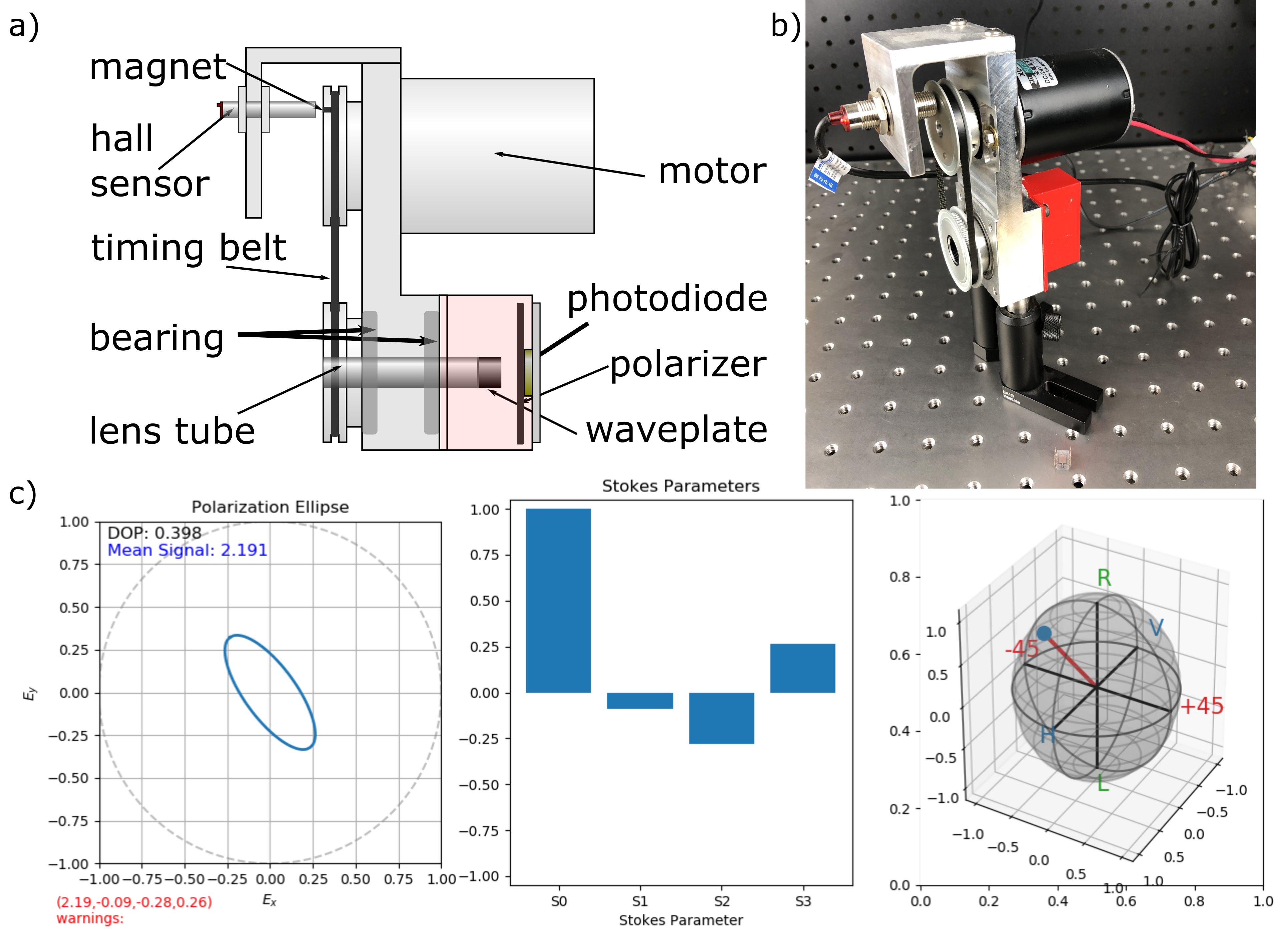
Figure 1: a) Mechanical design of our SWP. b) Photograph of the SWP mounted on an optics table. The photodiode signal goes directly to the Raspberry Pi with MCC118 ADC attached. c) Screen capture of the heads-up display shown by the analysis program while running.

2.2 Data Acquisition and Processing

In order to process the raw data, we use the API provided by the DAQ hat  to acquire a fixed number of samples for processing. We typically acquire 1000 samples at 20 ksps with a SWP rotation rate of 4500 to 5500 RPM, corresponding to several complete rotations.

To process this raw data, we divide the trace into $N$ segments corresponding to full rotations and assume a linear phase increase between trigger events. Each segment thus corresponds to equally spaced samples between $0$ and $2\pi$ rad. We numerically integrate each segment to extract the Fourier coefficients and use equation 1.2 to determine the Stokes parameters. We average the result of several segments to minimize statistical errors, and refresh the display at a rate of 4 Hz.

2.3 Calibration and Experimental Imperfections

2.3.1 Waveplate Alignment Offset Calibration

The angle $\theta$ in equation 1.2 refers to the physical angle between the transmission axis of the analysis polarizer and the fast axis of the waveplate. The angles of the magnetic trigger with respect to the polarization axis must therefore be known in order to set a phase reference of the trace. This may be accomplished with a simple procedure based on the fact that the $\cos 2\theta$ component of the signal is nominally precisely zero. If however, there is a phase offset $\theta\rightarrow\theta+\Delta\theta$, a nonzero cosine quadrature will appear since $\sin(\theta+\Delta\theta)=\cos\Delta\theta\sin\theta+\sin\Delta\theta\cos\theta$. We thus acquire a single rotation, and minimize the $\cos 2(\theta+\Delta\theta)$ curve over all possible phase delays $\Delta\theta$, recording the delay at which minimum value occurs. This is the offset angle between the magnetic sensor and the polarization axis which is used in reconstructing the polarization state. This entire process is automated with a simple script that takes seconds to run.

2.3.2 Imperfect Waveplates

The dispersive and birefringent nature of a waveplate leads to a wavelength dependent phase shift between slow and fast axes $\delta(\lambda)$ which can deviate greatly from the condition for a QWP of $\delta=\pi/2$. Referencing equation 1.2 we see that any deviation in $\delta$ will lead to an incorrect reconstruction of the polarization state, but knowing $\delta$, this can be corrected.

Our device allows for a fast, efficient measurement of the phase $\delta$, modulo $2\pi$. Since our system is monolithic containing its polarizer internally, we devise an in situ measurement of retardance which is insensitive to loss and finite polarization extinction ratio of commercial polarizers. By sending in light which is linearly polarized with respect to the internal polarizer, we expect an photodiode signal given by

$$V(\theta)=\left(\cos^{4}\theta+\sin^{4}\theta+2\cos^{2}\theta\sin^{2}\theta\cos\delta\right)V_{0}$$ (9)

…where $V_{0}$ is the voltage in the absence of the polarizer. The location of the maxima and minima can be used to extract the phase. Differentiating to find the extrema, we find the condition $\left[\sin 4\theta\left(\cos\delta-1\right)\right]=0$, so that $\theta=\frac{n\pi}{4}$. Noting that even $n$ yield maxima and odd $n$ give maxima, we can plug these values back into equation 9 to note:

$$\delta=\arccos\left(2\frac{V_{min}}{V_{max}}-1\right)$$ (10)

We perform this quick calibration before each use by means of an automated script. We find little day-to-day variation for a particular wavelength, but an large variation with wavelength. Our polarizer shows a phase of $\delta\approx\pi/2$ or $\lambda/4$ at $\lambda=780~{}$nm, but $\delta\approx 1.91$ at $\lambda=635~{}$nm corresponding to a $\lambda/3.29$-plate.

2.3.3 Technical Noise

Owing to the averaging process intrinsic to Fourier analysis, random errors tend to not affect the accuracy of our system. Non-random errors on the other hand, such as a constant dc offset will systematically bias the determination of the polarization state. This is evident from equation 1.2 where it is seen that an additional constant will lead to an overestimate of the sum of $S_{0}$ and $S_{3}$, generally underestimating the degree of polarization. A DC bias may be due either to unpolarized background light or dark current in the photodetector. This may be accounted for by directly subtracting the constant DC signal present while blocking the light source under test. This is performed on the fly with a Python script, and typically takes a few seconds, allowing for recalibration whenever the background conditions change.

Another source of experimental error which has plagued previous designs [13] is non-constant rotation of the QWP. In extracting the sine and cosine quadratures we are integrating along polarimeter angle and so this angle must be known at all points along the trace. This may be inferred by linear interpolation between triggers. If the angular velocity is not constant however, there will be a residual error. Since our SWP rotates at up to $6000$ RPM, the system is intrinsically inertially stable and significant changes to the angular speed will be gradual, over several periods. We verify this by observing the residual error from the fit of the measured voltage to the theoretical curve using a linearly polarized state.

3 Performance and Applications

3.1 Determining the Polarization State for Various Inputs

In order to test the functionality of our SWP system for partially and fully polarized light, we send in numerous known polarization states for calibration. We begin with incoherent, unpolarized light from a light emitting diode with $\lambda=663\pm 9$ nm. As we would expect, the output is unpolarized, showing a degree of polarization equal to $2.1\%$ (figure 2a).

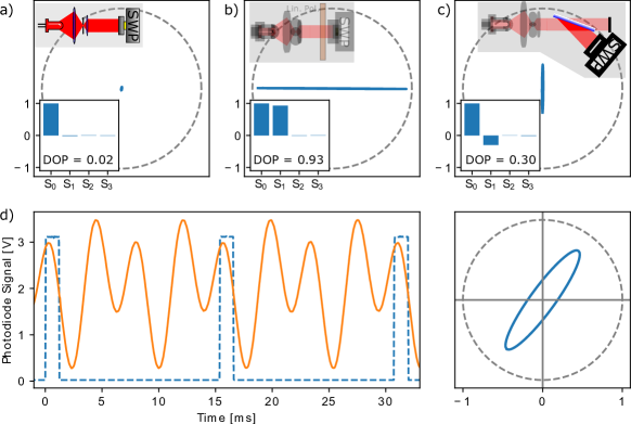
Figure 2: a) With unpolarized light such as an LED, the DOP is nearly 0. When a linear polarizer is included, the light is seen to be linearly polarized. c) Partial polarization by reflections via a glass microscope slide shows partial polarization. d) Shows the raw signal for several periods when a waveplate is placed after the microscope slide, with the corresponding ellipse to the right.

Next, we place a linear polarizer aligned horizontally after the LED and find a normalized Stokes vector of $(1.000,0.931,-0.031,0.006)$ with a degree of polarization of 93.1%  For a source of partially polarized light, we reflect the initially non-polarized LED light off a class microscope slide at an angle of $71^{\circ}$ with respect to the normal (figure 2c). As predicted from the Fresnel equations [14], we observed partially vertically polarized light. with a $DOP=29.8\%$. A general polarization state can be created by inserting a waveplate in the path of the partially polarized reflected light. This, along with the raw data is displayed in figure 2d.

3.2 Application: Extremely Affordable waveplates

A significant barrier to advanced experiments in atomic-optical physics in undergraduate teaching labs is the sheer number of optical components required. Certain experiments such as Pound-Drever Hall laser stabilization and Magneto optical trapping require many quarter wave plates, each of which can cost hundreds of dollars. It was noted in [15] that good quality waveplates may be constructed using overhead transparency paper as there is high transmission and suitable birefringence. By sending linear polarized light through the material in question and observing the polarization ellipse, our real-time SWP allows for a quick determination of regions with retardance appropriate for a QWP. Figure 3 shows a typical trace obtained with $S_{3}/S_{0}=-0.93$ corresponding to left handed, approximately circularly polarized light.

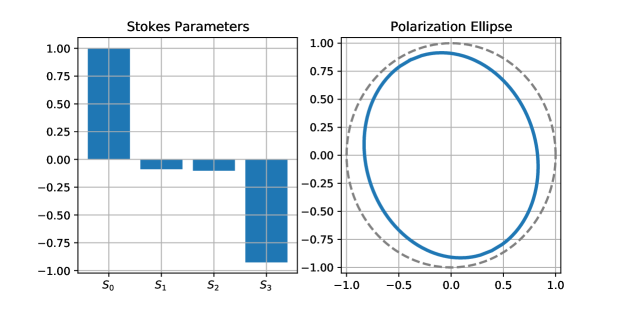
Figure 3: Stokes parameters (left) and polarization ellipse (right) for a sheet of transparency paper used as a quarter wave plate at $45^{\circ}$.

3.3 Application: Time Dependant polarization mapping

The real-time nature of our SWP allows for in-situ characterization of time dependent polarization states. Our acquisition rate is limited by the mechanical rotation rate of the device which is typically 100 Hz if we use one rotation of data. This sets the maximum polarization sample rate for our device for non-graphical operation, although a reduced rate is preferable for averaging and numerical accuracy. For graphical display, we find that the visualization on the Raspberry Pi becomes the bottle neck, and sets the update rate to around 10 frames per second. In figure 4a we shows the measured Stokes parameters for regular sample intervals while rotating a linear polarizer with an input circular polarizations state from a $650~{}$nm laser sent through a quarter waveplate.

We also can acquire and visualize the trajectory of a polarized state on the Poincaré sphere in real-time by keeping a buffer of the last $N$ points and plotting these along with the current location. Figure 4b shows such an example for acquiring data at 4 fps while rotating the transparency paper by hand.

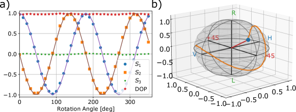
Figure 4: Time dependent measurements of the Polarizations state. a) Shows the measured Stokes parameters when an elliptically polarized beam is sent through a rotating polarizer. b) Shows the corresponding trajectory on the Poincaré sphere.

4 Conclusions

We have presented a real-time, fully integrated polarimeter based on affordable components that can be constructed by anyone with access to basic machining tools. We have described a single-shot calibration procedure that allows the use of an waveplate with non-ideal retardance, thus yielding a wide range of analysis wavelengths. By extending the analysis to partially polarized light, our device allows for an online visualization of an input optical state of arbitrary polarization. This has potential for visual demonstration in educational settings as well for providing a convenient heads-up display for in-lab calibration procedures. We also envision application in determining polarization dependent physical quantities such as concentration of optically active substances in a solution and stress induced birefringence metrology.

Acknowledgments: We thank the University of Victoria, Faculty of Science Machine Shop and the Dept. of Physics & Astronomy Electronics Shop for assistance with the design and construction of the device. We gratefully acknowledge internal support from Department of Physics & Astronomy at the University of Victoria for funding this research.

References

- [1] S. Garcia, J. Reichel, and R. Long, “Improving the lifetime in optical microtraps by using elliptically polarized dipole light,” \JournalTitlePhysical Review A 97, 023406 (2018).
- [2] J. Marshall, D. Cotton, K. Bott, S. Ertel, G. Kennedy, M. Wyatt, C. del Burgo, O. Absil, J. Bailey, and L. Kedziora-Chudczer, “Polarization measurements of hot dust stars and the local interstellar medium,” \JournalTitleThe Astrophysical Journal 825, 124 (2016).
- [3] M. Losurdo, M. Bergmair, G. Bruno, D. Cattelan, C. Cobet, A. de Martino, K. Fleischer, Z. Dohcevic-Mitrovic, N. Esser, M. Galliet et al., “Spectroscopic ellipsometry and polarimetry for materials and systems analysis at the nanometer scale: state-of-the-art, potential, and perspectives,” \JournalTitleJournal of Nanoparticle Research 11, 1521–1554 (2009).
- [4] T. Capelle, Y. Tsaturyan, A. Barg, and A. Schliesser, “Polarimetric analysis of stress anisotropy in nanomechanical silicon nitride resonators,” \JournalTitleApplied Physics Letters 110, 181106 (2017).
- [5] D. Goldstein, Polarized Light, 2nd ed. (Marcell Dekker Inc., 2003).
- [6] M. Born and E. Wolf, Principles of optics: electromagnetic theory of propagation, interference and diffraction of light (Elsevier, 2013).
- [7] B. Zhao, X.-B. Hu, V. Rodríguez-Fajardo, Z.-H. Zhu, W. Gao, A. Forbes, and C. Rosales-Guzmán, “Real-time stokes polarimetry using a digital micromirror device,” \JournalTitleOptics express 27, 31087–31093 (2019).
- [8] R. D. Hawley, J. Cork, N. Radwell, and S. Franke-Arnold, “Passive broadband full stokes polarimeter using a fresnel cone,” \JournalTitleScientific reports 9, 1–8 (2019).
- [9] J. M. Bueno, “Polarimetry using liquid-crystal variable retarders: theory and calibration,” \JournalTitleJournal of Optics A: Pure and Applied Optics 2, 216 (2000).
- [10] H. G. Berry, G. Gabrielse, and A. Livingston, “Measurement of the stokes parameters of light,” \JournalTitleApplied optics 16, 3200–3205 (1977).
- [11] B. Schaefer, E. Collett, R. Smyth, D. Barrett, and B. Fraher, “Measuring the stokes polarization parameters,” \JournalTitleAmerican Journal of Physics 75, 163–168 (2007).
- [12] S. Bobach, A. Hidic, J. J. Arlt, and A. J. Hilliard, “Note: A portable rotating waveplate polarimeter,” \JournalTitleReview of Scientific Instruments 88, 036101 (2017).
- [13] S. Arnoldt, “Rotating quarter-wave plate stokes polarimeter,” (2011).
- [14] E. Hecht, Optics (Pearson, 2017), vol. 5, pp. 358–364.
- [15] C. Wieman, G. Flowers, and S. Gilbert, “Inexpensive laser cooling and trapping experiment for undergraduate laboratories,” \JournalTitleAmerican Journal of Physics 63, 317–330 (1995).