A partially collapsed sampler for unsupervised nonnegative spike train restoration

Abstract

In this paper the problem of restoration of non-negative sparse signals is addressed in the Bayesian framework. We introduce a new probabilistic hierarchical prior, based on the Generalized Hyperbolic (GH) distribution, which explicitly accounts for sparsity. This new prior allows on the one hand, to take into account the non-negativity. And on the other hand, thanks to the decomposition of GH distributions as continuous Gaussian mean-variance mixture, allows us to propose a partially collapsed Gibbs sampler (PCGS), which is shown to be more efficient in terms of convergence time than the classical Gibbs sampler.

1 Introduction

This paper tackles the restoration of a sparse non-negative signal, observed though a linear operator and corrupted by additive white noise. The $N\times 1$ observed signal ${\boldsymbol{y}}$ can be written as ${\boldsymbol{y}}={\mathbf{H}}{\boldsymbol{z}}+{\boldsymbol{\epsilon}}$, where ${\boldsymbol{z}}$ is the $K\times 1$ sparse non-negative signal, ${\mathbf{H}}$ is a $N\times K$ matrix and ${\boldsymbol{\epsilon}}$ models the perturbations.

In the literature, sparse signal restoration problems arise in different fields such as reflection seismology, astronomy and compressed sensing. The objective is to find a sparse representation of a given signal ${\boldsymbol{y}}$ that is a linear combination of a limited number of elements (atoms) taken from a given dictionary ${\mathbf{H}}$. This problem is often referred to as subset selection because it consists in selecting a subset of columns of ${\mathbf{H}}$. Mathematically, this can be formulated as the minimization of the squared error $\left\|{\boldsymbol{y}}-{\mathbf{H}}{\boldsymbol{z}}\right\|^{2}$ subject to $\left\|{\boldsymbol{z}}\right\|_{0}<S$, where $\left\|\cdot\right\|$ and $\left\|\cdot\right\|_{0}$ respectively stands for the Euclidean norm, and the $\ell_{0}$ pseudo-norm. This yields a combinatorial discrete problem known to be NP-hard [18].

One alternative is the convex relaxation of the problem which substitutes the $\ell_{0}$ pseudo-norm by the $\ell_{1}$ norm [9, 11], the sparsity of the solutions coming from the non smooth character of the $\ell_{1}$ norm at zero. Greedy algorithms, such as Matching Pursuit and its improved versions Orthogonal Matching Pursuit and Orthogonal Least Squares, form another class of methods. The main idea is to iteratively enlarge or reduce by one the set of active atoms.

Non-negative adaptations have been proposed for both convex relaxation and greedy algorithms. For example, the $\ell_{1}$ relaxation can be easily extended to the non-negative setting [1, 12]. Non-negative extensions of greedy algorithms have been also introduced [7, 22, 19].

On the other hand, a hierarchical Bayesian model which explicitly accounts for sparsity has been proposed for spike deconvolution, namely the Bernoulli-Gaussian (BG) model [16, 8]. Deterministic optimization algorithms [8] and Markov chain Monte Carlo techniques (MCMC) [10] are used to compute, respectively, the Maximum a Posteriori (MAP) and the Posterior Mean (PM) estimators. In the sparse train deconvolution context, the aforementioned methods have no theoretical guarantee regarding the exact recovery of the signal. However, the PM estimator has been shown empirically to give better results than greedy algorithms and convex relaxation [4]. Moreover, the Bayesian framework allows one to estimate the model hyper-parameters (unsupervised case).

In the MCMC framework, a non-negative adaptation of the BG model was studied in [17], based on a Bernoulli-Truncated-Gaussian (BTG) model. Vector ${\boldsymbol{z}}$ is modelled as a couple of variables $({\boldsymbol{q}},{\boldsymbol{x}})$ i.e., independent, identically distributed (i.i.d.) Bernoulli variables ${\boldsymbol{q}}_{k}$, i.i.d. centered truncated Gaussian amplitudes ${\boldsymbol{x}}_{k}$ when ${\boldsymbol{q}}_{k}=1$, and ${\boldsymbol{x}}_{k}=0$ when ${\boldsymbol{q}}_{k}=0$. Posterior Mean estimation of ${\boldsymbol{q}}$ and ${\boldsymbol{x}}$ is then obtained using an MCMC method. The latter yields satisfactory results, but it requires a high computational cost. In [20], some strategies and tools are presented to construct a partially collapsed Gibbs sampler (PCGS) with known stationary distribution and faster convergence. The partially collapsed Gibbs sampler substitutes some of the posterior conditional distributions with marginal distributions of the joint posterior. Such a technique has proven its efficiency for BG deconvolution [3, 13] where the amplitudes ${\boldsymbol{x}}$ can be marginalized out from the joint posterior thanks to their Gaussianity. Unfortunately, partially collapsed sampling cannot be as easily adapted to the context of non-negative BG restoration.

The aim of this paper is to implement partially collapsed sampling in the context of non-negative sparse restoration. Our main contribution is to propose a new prior based on the Generalized Hyperbolic (GH) distribution. On the one hand, the proposed prior mimics the BTG prior to take into account the non-negativity. On the other hand, the decomposition of GH distributions as continuous Gaussian mean-variance mixture allows us to marginalize the amplitudes, enabling the construction of a partially collapsed Gibbs sampler which is shown hereafter to converge more rapidly than the BTG version.

The organization of this paper is as follows. An overview of the Generalized Hyperbolic distribution and its properties are given in Section 2. Section 3 introduces the Bernoulli-Generalized-Hyperbolic (BGH) model in the Bayesian framework. Its corresponding partially collapsed Gibbs sampler is presented in Section 4. Simulation results are given in Section 5 to compare the BGH and the BTG samplers both in terms of signal restoration and convergence. Finally, conclusions are drawn in Section 6.

2 Generalized hyperbolic distributions

2.1 Description and properties

Generalized Hyperbolic (GH) laws form a five-parameter family $(\lambda,\alpha,\beta,\delta,\mu)$ introduced by Barndorff-Nilsen in [2]. If a random variable $X\sim\mathit{GH}(\lambda,\alpha,\beta,\delta,\mu)$ then its probability density is given by

$$p_{X}(x)=\frac{(\gamma/\delta)^{\lambda}}{\sqrt{2\pi}K_{\lambda}(\delta\gamma)}\frac{K_{\lambda-\frac{1}{2}}(\alpha\sqrt{\delta^{2}+(x-\mu)^{2}})}{(\sqrt{\delta^{2}+(x-\mu)^{2}}/\alpha)^{\frac{1}{2}-\lambda}}e^{\beta(x-\mu)},$$

where $\gamma^{2}=\alpha^{2}-\beta^{2}$ and $K_{\lambda}$ is the modified Bessel function of third kind. We will take advantage of two interesting properties of the GH distributions:

• GH distributions have the property of being invariant under affine transformations. If $X\sim\mathit{GH}(\lambda,\alpha,\beta,\delta,\mu)$, then $Y=aX+b\sim\mathit{GH}(\lambda,\alpha/a,\beta/a,a\delta,a\mu+b)$.

• They can be expressed as continuous normal mean-variance mixtures

$$p_{X}(x)=\int_{0}^{\infty}p_{X|W}(x|w)\,p_{W}(w)\,dw$$

where $X|W\sim\mathcal{N}(\mu+\beta W,W)$ and each random variance $W$ follows a Generalised Inverse Gaussian [15] distribution $\mathit{GIG}(\lambda,\gamma,\delta)$ with the probability density

$$p_{W}(w)=\frac{(\gamma/\delta)^{\lambda}}{2K_{\lambda}(\delta\gamma)}w^{\lambda-1}\exp\left(-\frac{\raisebox{-1.0pt}{$1$}}{2}\left(\delta^{2}w^{-1}+\gamma^{2}w\right)\right),~{}w>0.$$

Therefore, a GH random variable can be seen as a hierarchical model: in order to generate a GH sample, a random variance $W\sim\mathit{GIG}(\lambda,\gamma,\delta),$ is first drawn, and then $X|W$ with a normal distribution $\mathcal{N}(\mu+\beta W,W)$.

2.2 Truncated Gaussian approximation

One easy way to estimate the parameters of the GH distribution that best approximate a given distribution, is to first generate $N$ samples ${\boldsymbol{s}}=\{{\boldsymbol{s}}_{1},\cdots,{\boldsymbol{s}}_{N}\}$ according to it, and then to estimate the GH parameters using the Maximum-likelihood estimator [5]. As $N\to\infty$, this is equivalent to minimizing the Kullback-Leibler divergence between the two distributions.

Let ${\boldsymbol{\nu}}_{\mathcal{N}}=(\lambda_{\mathcal{N}},\alpha_{\mathcal{N}},\beta_{\mathcal{N}},\delta_{\mathcal{N}},\mu_{\mathcal{N}})$ denote the parameters that best approximate the truncated version of the normalized Gaussian $\mathcal{N}^{+}(0,1)$ with the GH distribution:

$$X\sim\mathit{GH}({\boldsymbol{\nu}}_{\mathcal{N}})\approx\mathcal{N}^{+}(0,1),$$ (1)

Since the GH distribution is closed under affine transformations, we can approximate the truncated version of any other centered Gaussian $\mathcal{N}^{+}(0,\sigma_{x}^{2})$ as follows:

$$\mathit{GH}(\lambda_{\mathcal{N}},\alpha_{\mathcal{N}}/\sigma_{x},\beta_{\mathcal{N}}/\sigma_{x},\delta_{\mathcal{N}}\sigma_{x},\mu_{\mathcal{N}}\sigma_{x})\approx\mathcal{N}^{+}(0,\sigma_{x}^{2}).$$ (2)

As the parameters of this distribution are fixed given $\sigma_{x}$, we will write $\mathit{GH}_{\mathcal{N}}(\sigma_{x}^{2})$ for sake of simplicity. Similarly, we write $\mathit{GIG}_{\mathcal{N}}(\sigma_{x}^{2})$ instead of $\mathit{GIG}(\lambda_{\mathcal{N}},\gamma_{\mathcal{N}}/\sigma_{x},\delta_{\mathcal{N}}\sigma_{x})$.

3 Bayesian framework

3.1 Bernoulli-Generalized-Hyperbolic prior

In the following we will consider that ${\boldsymbol{z}}=({\boldsymbol{q}},{\boldsymbol{x}})$ where ${\boldsymbol{q}}_{k}\sim\mathcal{B}(\lambda),\forall k=1,\cdots,K$ and:

$$\begin{split}{\boldsymbol{x}}_{k}|{\boldsymbol{q}}_{k}=1&\sim\left\{\begin{tabular}[]{l}${\boldsymbol{w}}_{k}\sim\mathit{GIG}_{\mathcal{N}}(\sigma_{x}^{2})$\\ ${\boldsymbol{x}}_{k}|{\boldsymbol{w}}_{k}\sim\mathcal{N}(\sigma\mu_{\mathcal{N}}+{\boldsymbol{w}}_{k}\beta_{\mathcal{N}}/\sigma,{\boldsymbol{w}}_{k}),$\end{tabular}\right.\\ {\boldsymbol{x}}_{k}|{\boldsymbol{q}}_{k}=0&\sim\delta({\boldsymbol{x}}_{k}),\\ \end{split}$$

leading to the Bernoulli-Generalized-Hyperbolic prior.

3.2 Posterior distribution

We consider an independent noise sequence $\{{\boldsymbol{\epsilon}}_{k}\}_{k}$, zero-mean, Gaussian, with variance $\sigma^{2}$. The posterior distribution can be written as follows:

$$p({\boldsymbol{q}},{{\boldsymbol{x}}},{\boldsymbol{w}}|{\boldsymbol{y}})\propto\exp\left(-\frac{\raisebox{-1.0pt}{$1$}}{2\sigma^{2}}\left\|{\boldsymbol{y}}-\overline{{\mathbf{H}}}\overline{{\boldsymbol{x}}}\right\|^{2}\right)p({\boldsymbol{q}},{{\boldsymbol{x}}},{\boldsymbol{w}})$$ (3)

where $\overline{{\boldsymbol{x}}}$ gathers the elements of the vector ${\boldsymbol{x}}$ for which ${\boldsymbol{q}}_{k}=1$ and similarly $\overline{{\mathbf{H}}}$ concatenates the columns of the matrix ${\mathbf{H}}$ for which ${\boldsymbol{q}}_{k}=1$.

For an unsupervised estimation, a prior distribution can be introduced for the hyper-parameters ${\boldsymbol{\theta}}=[\lambda,\sigma^{2},\sigma_{x}^{2}]$ independent of the other parameters, and the posterior distribution can be written:

$$p({\boldsymbol{q}},{\boldsymbol{x}},{\boldsymbol{w}},{\boldsymbol{\theta}}|{\boldsymbol{y}})\propto p({\boldsymbol{q}},{\boldsymbol{x}},{\boldsymbol{w}}|{\boldsymbol{y}},{\boldsymbol{\theta}})p({\boldsymbol{\theta}})$$ (4)

3.3 Partially marginalized posterior distribution

From (4), it is straightforward to deduce that $\overline{{\boldsymbol{x}}}|{\boldsymbol{q}},{\boldsymbol{w}},{\boldsymbol{y}},{\boldsymbol{\theta}}$ follows a multivariate Gaussian $\mathcal{N}({\boldsymbol{\eta}},{\boldsymbol{\Gamma}})$, with

$${\boldsymbol{\eta}} =\sigma^{-2}{\boldsymbol{\Gamma}}\overline{{\mathbf{H}}}^{T}{\boldsymbol{y}}+{\boldsymbol{\Gamma}}{{\mathbf{W}}}^{-1}{{\boldsymbol{\mu}}}_{x},$$

$${\boldsymbol{\Gamma}} =\bigl{(}\sigma^{-2}\overline{{\mathbf{H}}}^{T}\overline{{\mathbf{H}}}+{{\mathbf{W}}}^{-1}\bigr{)}^{-1},$$

where ${{\boldsymbol{\mu}}}_{x}=\sigma\mu_{\mathcal{N}}\mathbb{1}_{L}+\frac{\beta_{\mathcal{N}}}{\sigma}{{\boldsymbol{w}}}$ and $L=\sum_{k}{\boldsymbol{q}}_{k}$. As a consequence, one can easily calculate the marginalized posterior distribution with respect to ${\boldsymbol{x}}$

$$p({\boldsymbol{q}},{\boldsymbol{w}},{\boldsymbol{\theta}}|{\boldsymbol{y}}) \propto|{\mathbf{B}}|^{-1/2}~{}P({\boldsymbol{q}}|\lambda)p({\boldsymbol{\theta}})\prod_{k}p({\boldsymbol{w}}_{k})$$

$$\times \exp\left(-\frac{\raisebox{-1.0pt}{$1$}}{2}({\boldsymbol{y}}^{T}{\mathbf{B}}^{-1}{\boldsymbol{y}}+{\boldsymbol{\mu}}_{x}^{T}{\mathbf{C}}^{-1}{\boldsymbol{\mu}}_{x}-2{\boldsymbol{y}}^{T}{\mathbf{D}}{\boldsymbol{\mu}}_{x})\right)$$

with ${\mathbf{W}}={\mathrm{diag}}\{{\boldsymbol{w}}\}$ and:

$$\begin{array}[]{lll|c|}{\mathbf{B}}^{-1}&=&\sigma^{-2}{\mathbf{I}}-\sigma^{-4}\overline{{\mathbf{H}}}{\boldsymbol{\Gamma}}\overline{{\mathbf{H}}}^{T}&(N\times N)\\ {\mathbf{C}}^{-1}&=&{\mathbf{W}}^{-1}-{\mathbf{W}}^{-1}{\boldsymbol{\Gamma}}{\mathbf{W}}^{-1}&(L\times L)\\ {\mathbf{D}}&=&\sigma^{-2}\overline{{\mathbf{H}}}{\boldsymbol{\Gamma}}{\mathbf{W}}^{-1}&(N\times L)\end{array}$$

4 Partially Collapsed Gibbs Sampler

While sampling ${\boldsymbol{x}}|{\boldsymbol{q}},{\boldsymbol{w}}$ is an easy task ($\overline{{\boldsymbol{x}}}$ is Gaussian), sampling ${\boldsymbol{q}}$ and ${\boldsymbol{w}}$ need to be considered in a special framework as the variable ${\boldsymbol{w}}_{k}$ is defined only if ${\boldsymbol{q}}_{k}=1$ which implies that the posterior distribution is defined in a space with a varying dimension. A general framework for Metropolis-Hastings algorithms was introduced in [14], namely the Reversible-Jump (RJ) MCMC methods, in order to manage jumps between subspaces of different dimensions in stochastic sampling algorithms. The sampling strategy adopted here is as follows (Algorithm 1). At each iteration $i$, first sample ${\boldsymbol{q}}^{(i)}$ and ${\boldsymbol{w}}^{(i)}$ using the RJ-MCMC framework as shown in Algorithm 2 (see 4.1 for explanations), then sample ${\boldsymbol{x}}^{(i)}|{\boldsymbol{q}}^{(i)},{\boldsymbol{w}}^{(i)}$, and finally sample the hyper-parameters ${\boldsymbol{\theta}}$ according to their posterior.

At each iteration $i$:

1. for all $k$ in $1,\cdots,K$:

   1. draw ${\boldsymbol{q}}_{k},{\boldsymbol{w}}_{k}|{\boldsymbol{q}}_{-k},{\boldsymbol{w}}_{-k},{\boldsymbol{\theta}},{\boldsymbol{y}}$ according to

      Algorithm 2

2. draw ${\boldsymbol{x}}|{\boldsymbol{q}},{\boldsymbol{w}},{\boldsymbol{\theta}},{\boldsymbol{y}}$ (Gaussian distribution)

3. draw ${\boldsymbol{\theta}}|{\boldsymbol{q}},{\boldsymbol{w}},{\boldsymbol{x}},{\boldsymbol{y}}$ according to their conditional

   posterior distributions

Algorithm 1 Partially collapsed Gibbs sampler

4.1 Reversible-Jump step

For the problem considered here, two states can be distinguished; whether ${\boldsymbol{q}}_{k}=1$ and ${\boldsymbol{w}}_{k}$ is defined, or ${\boldsymbol{q}}_{k}=0$ and ${\boldsymbol{w}}_{k}$ is not defined. The RJ-MCMC framework allows to jump between these two states using the moves hereafter:

1. Birth: from ${\boldsymbol{q}}_{k}=0$ propose ${\boldsymbol{q}}_{k}^{\prime}=1,{\boldsymbol{w}}_{k}^{\prime}$,

2. Death: from ${\boldsymbol{q}}_{k}=1,{\boldsymbol{w}}_{k}$ propose ${\boldsymbol{q}}_{k}^{\prime}=0$,

3. Update: from ${\boldsymbol{q}}_{k}=1,{\boldsymbol{w}}_{k}$ propose ${\boldsymbol{q}}_{k}^{\prime}=1,{\boldsymbol{w}}_{k}^{\prime}$.

note that the move from ${\boldsymbol{q}}_{k}=0$ to ${\boldsymbol{q}}_{k}^{\prime}=0$ is not of interest as this proposal is always accepted, and cannot introduce any change.

In the following, we denote by $p_{uu^{\prime}}$ the probability of proposing a move from the state $u$ to $u^{\prime}$. Since we have chosen to systematically propose a birth move when ${\boldsymbol{q}}_{k}=0$ then $p_{01}=1$. Otherwise, when ${\boldsymbol{q}}_{k}=1$, it is reasonable to randomly propose either a death or an update move with equal probability $p_{10}=p_{11}=\frac{1}{2}$.

The ${\boldsymbol{w}}_{k}^{\prime}$ candidates are proposed according to the following proposal distributions. When a birth move is chosen, it seems natural to propose ${\boldsymbol{w}}_{k}^{\prime}$ according to its prior distribution $q_{01}({\boldsymbol{w}}_{k}^{\prime})\sim\mathit{GIG}_{\mathcal{N}}(\sigma_{x}^{2})$. Also, if a death is selected the variable ${\boldsymbol{w}}_{k}^{\prime}$ disappears meaning that the proposal is deterministic, hereafter for notational convenience we will write $q_{10}({\boldsymbol{w}}_{k}^{\prime})=1$ (for more details, one may refer to [21, Remark 4.2]) . Finally, for the update move, a mix of two proposal distributions is considered: the first one is the prior distribution $q^{(1)}_{11}({\boldsymbol{w}}_{k}^{\prime})\sim\mathit{GIG}_{\mathcal{N}}(\sigma_{x}^{2})$ allowing a better exploration of the feasible domain of ${\boldsymbol{w}}_{k}$, while the second was empirically determined to maximize the acceptance probability, and thus to produce a better exploration of the posterior, according to:

$$q^{(2)}_{11}({\boldsymbol{w}}_{k}^{\prime})\sim\mathit{GIG}\left(\lambda_{\mathcal{N}}-\frac{\raisebox{-1.0pt}{$1$}}{2},\frac{\raisebox{-1.0pt}{$1$}}{\sigma_{x}}\sqrt{\gamma_{\mathcal{N}}^{2}+\beta_{\mathcal{N}}^{2}},\sigma_{x}\sqrt{\delta_{\mathcal{N}}^{2}+\mu_{\mathcal{N}}^{2}}\right)$$

In practice, we have noticed that alternating between these two proposals with equal probabilities improves the mixing property of the Markov chain. The candidates are accepted according to the following probability:

$$\alpha_{uu^{\prime}}=\min\left[1,\frac{p({\boldsymbol{y}},{\boldsymbol{q}}^{\prime},{\boldsymbol{w}}^{\prime})\,p_{u^{\prime}u}\,q_{u^{\prime}u}({\boldsymbol{w}}_{k}^{\prime})}{p({\boldsymbol{y}},{\boldsymbol{q}},{\boldsymbol{w}})\,p_{uu^{\prime}}\,q_{u^{\prime}u}({\boldsymbol{w}}_{k})}\right].$$ (5)

This ensures the reversibility, and thus the invariance of the Markov chain with respect to the posterior distribution (see [14, 21]). Direct evaluation of (5) is inefficient from the computational viewpoint. Therefore, we have adapted and extended the numerical implementation technique introduced in [13] to reduce the computation and memory load. A key point is to recursively handle Cholesky factors instead of matrices ${\mathbf{B}}$, ${\mathbf{C}}$ and ${\mathbf{D}}$. Due to lack of space, calculation details cannot be given here.

if ${\boldsymbol{q}}_{k}$ = 0 then

       – propose a birth move:

      ${\boldsymbol{q}}_{k}^{\prime}=1$ and ${\boldsymbol{w}}_{k}^{\prime}\sim q_{01}({\boldsymbol{w}}_{k}^{\prime})$, then accept the proposition with probability $\alpha_{01}$.

else

       – with probability $p_{10}$ propose a death move:

      ${\boldsymbol{q}}_{k}^{\prime}=0$ and ${\boldsymbol{w}}_{k}^{\prime}=\O,$ then accept the proposition with probability $\alpha_{10}$.

      – with probability $p_{11}=1-p_{10}$ propose an update move:

      ${\boldsymbol{q}}_{k}^{\prime}=1$ and ${\boldsymbol{w}}_{k}^{\prime}\sim q^{(1)}_{11}({\boldsymbol{w}}_{k}^{\prime})$ or ${\boldsymbol{w}}_{k}^{\prime}\sim q^{(2)}_{11}({\boldsymbol{w}}_{k}^{\prime})$ with a probability $\frac{1}{2},$ then accept the proposition with probability $\alpha_{11}$.

end if

Algorithm 2 Sampling ${\boldsymbol{q}}_{k}$ and ${\boldsymbol{w}}_{k}$ using the RJ framework

5 Simulation tests

In this section, our goal is to compare the BTG and BGH samplers, both in terms of signal restoration and convergence rate. We have designed a test scenario similar to the one used in [17]. The observed signal ${\boldsymbol{y}}$ (of length $N=84$) is corrupted by Gaussian noise with $\sigma^{2}=5.5\times 10^{-7},$ corresponding to a signal-to-noise ratio (SNR) of $10$ dB (Fig 1), and the impulse response was chosen to be of length $K=21$ and of the following form ${\boldsymbol{h}}_{n}=\frac{\raisebox{-1.0pt}{$s^{2}$}}{s^{2}+n^{2}}$ where $s$ is an unknown scale parameter. Here, we propose to sample $s$ using a Metropolis-Hastings step. Furthermore, we consider an unsupervised situation where the hyper-parameters ${\boldsymbol{\theta}}=[\lambda,\sigma_{x}^{2}]^{T}$ are also unknown and sampled, while the noise variance is assumed to be known.

$h_{n}$
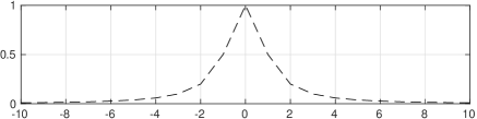
	$n$
$y_{n}$	\psfrag{Noiseless data}{\tiny Noiseless data}\psfrag{Noisy data}{\tiny Noisy data}\includegraphics[width=227.90501pt]{./figs/SSP_MPSRF_QWHXLV_Z}
	$n$

Fig. 1: Impulse response $h_{n}$ and simulated data $y_{n}$ for the test scenario.

To empirically compare the convergence speed of the different samplers, we have used Brooks and Gelman’s iterated graphical method to assess convergence [6]. This diagnostic method is based upon the covariance estimation of $J$ independent Markov chains of equal length $I$: $\{{\mathbf{X}}_{j,i};j=1,\cdots,J;i=1,\cdots,I\}$. The intra-chain and inter-chain variances that characterize the convergence behaviour, are defined as covariance matrix averages:

$${\mathbf{V}}_{\text{intra}} =\frac{\raisebox{-1.0pt}{$1$}}{J(I-1)}\sum_{j}\sum_{i}\left({\mathbf{X}}_{j,i}-\overline{{\mathbf{X}}}_{j}\right)\left({\mathbf{X}}_{j,i}-\overline{{\mathbf{X}}}_{j}\right)^{T}$$

$${\mathbf{V}}_{\text{inter}} =\frac{\raisebox{-1.0pt}{$1$}}{J-1}\sum_{j}\left(\overline{{\mathbf{X}}}_{j}-\overline{{\mathbf{X}}}\right)\left(\overline{{\mathbf{X}}}_{j}-\overline{{\mathbf{X}}}\right)^{T}$$

where $\overline{{\mathbf{X}}}_{j}$ and $\overline{{\mathbf{X}}}$ denote the local and the global mean of the chains respectively. Brooks and Gelman [6] proposed to evaluate the multivariate potential scale reduction factor (MPSRF) given by

$$R=\frac{I-1}{I}+\frac{J+1}{J}\lambda\left({\mathbf{V}}_{\text{intra}}^{-1}{\mathbf{V}}_{\text{inter}}\right)$$

where $\lambda({\mathbf{A}})$ denotes the largest eigenvalue of the matrix ${\mathbf{A}}$. Convergence is diagnosed when the MPSRF is close to one. As suggested in [6], we have chosen $R<1.2$.

Fig. 2 shows the Posterior Mean (PM) estimates of ${\boldsymbol{x}}$ produced by both samplers. They are of similar quality, which indicates that the approximation method of the truncated Gaussian by the GH distribution is effective.

$x_{n}$
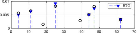
	$n$
$x_{n}$
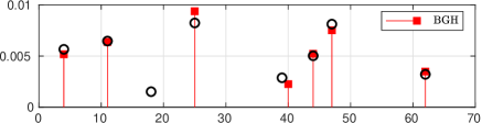
	$n$

Fig. 2: Estimation results at convergence of ${{\boldsymbol{x}}}$ for the BTG (top figure) and BGH (bottom figure) compared to its true value (black circles).

Fig. 3 gives the MPSRF of the variables ${\boldsymbol{q}}$ in logarithmic scale for both samplers, as a function of time. Simulations were run using MATLAB on a computer with Intel Xeon E5-2680 processors with a CPUs clocked at 2.8 GHz. To evaluate the MPSRF, each chain is divided into batches of $b$ samples, and the MPSRF is calculated upon the second halves of the Markov chains $\{{\mathbf{X}}_{j,i}\},i=1,\cdots,kb$ for increasing lengths $kb$. As recommended in [6], we have chosen $b\approx\frac{I}{20}$, where $I$ is the length of the Markov chain. Whereas the BTG sampler needs around 36000 iterations to converge, the proposed BGH converges in about 1250 iterations, thanks to partially collapsed sampling. In terms of computing time, the acceleration factor is still significant but more modest (8 versus 30 seconds), since BGH iterations are more complex than that of BTG, despite the fact that the former have been optimized using recursive Cholesky factor updatings. Finally, let us stress that the considered numerical test corresponds to a problem of moderate complexity. For problems of increasing complexity, the relative efficiency of the partially collapsed sampler is expected to increase compared to the standard sampler, according to [13].

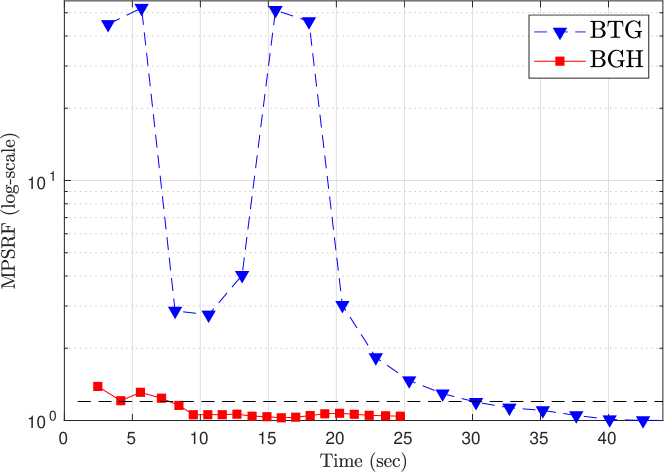
Fig. 3: Evolution of MPSRF (in log scale) of the BTG and BGH samplers. The horizontal line corresponds to the 1.2 threshold.

6 Conclusion

We have presented a new probabilistic hierarchical model for solving non-negative sparse signal restoration problems in an unsupervised way using MCMC methods. Thanks to the properties of GH distributions in terms of Gaussian mixture decomposition, the proposed model allows us to marginalize the amplitudes and to devise a partially collapsed Gibbs sampler, with improved mixing properties compared to the standard Gibbs sampler.

An interesting perspective would be to extend this approach based on Gaussian mixture decomposition and partially collapsed sampling to other restoration problems incorporating more general constraints than non-negativity.

References

- [1] I. Barbu and C. Herzet. A new approach for volume reconstruction in TomoPIV with the alternating direction method of multipliers. Measurement Science and Technology, 27(10):104002, Oct. 2016.
- [2] O. Barndorff-Nielsen. Exponentially Decreasing Distributions for the Logarithm of Particle Size. Proceedings of the Royal Society A: Mathematical, Physical and Engineering Sciences, 353(1674):401–419, Mar. 1977.
- [3] M. Boudineau, H. Carfantan, S. Bourguignon, and M. Bazot. Sampling schemes and parameter estimation for nonlinear Bernoulli-Gaussian sparse models. In 2016 IEEE Statistical Signal Processing Workshop (SSP), pages 1–5, Palma de Mallorca, Spain, June 2016.
- [4] S. Bourguignon, C. Soussen, H. Carfantan, and J. Idier. Sparse deconvolution: Comparison of statistical and deterministic approaches. In 2011 IEEE Statistical Signal Processing Workshop (SSP), pages 317–320, Nice, France, June 2011.
- [5] W. Breymann and D. Lüthi. ghyp: A package on generalized hyperbolic distributions. Manual for R Package ghyp, 2013.
- [6] S. P. Brooks and A. Gelman. General methods for monitoring convergence of iterative simulations. Journal of Computational and Graphical Statistics, 7(4):434–455, 1998.
- [7] A. M. Bruckstein, M. Elad, and M. Zibulevsky. On the Uniqueness of Nonnegative Sparse Solutions to Underdetermined Systems of Equations. IEEE Transactions on Information Theory, 54(11):4813–4820, Nov. 2008.
- [8] F. Champagnat, Y. Goussard, and J. Idier. Unsupervised deconvolution of sparse spike trains using stochastic approximation. IEEE Transactions on Signal Processing, 44(12):2988–2998, Dec. 1996.
- [9] S. S. Chen, D. L. Donoho, and M. A. Saunders. Atomic decomposition by basis pursuit. SIAM Review, 43(1):129–159, 2001.
- [10] Q. Cheng, R. Chen, and T.-H. Li. Simultaneous wavelet estimation and deconvolution of reflection seismic signals. IEEE Transactions on Geoscience and Remote Sensing, 34(2):377–384, Mar. 1996.
- [11] D. L. Donoho and Y. Tsaig. Fast solution of -norm minimization problems when the solution may be sparse. IEEE Transactions on Information Theory, 54(11):4789–4812, Nov. 2008.
- [12] B. Efron, T. Hastie, I. Johnstone, and R. Tibshirani. Least angle regression. Annals of Statistics, 32(2):407–451, 2004.
- [13] D. Ge, J. Idier, and E. Le Carpentier. Enhanced sampling schemes for MCMC based blind Bernoulli–Gaussian deconvolution. Signal Processing, 91(4):759–772, Apr. 2011.
- [14] P. J. Green. Reversible jump MCMC computation and Bayesian model determinaion. Biometrika, 82:711–732, 1995.
- [15] B. Joergensen. Statistical Properties of the Generalized Inverse Gaussian. Number 9 in Lecture Notes in Statistics. Springer-Verlag, New York, Heidelberg, Berlin, 1982.
- [16] J. Kormylo and J. Mendel. Maximum likelihood detection and estimation of Bernoulli - Gaussian processes. IEEE Transactions on Information Theory, 28(3):482–488, May 1982.
- [17] V. Mazet, J. Idier, and D. Brie. Déconvolution impulsionnelle positive myope. In Actes 20e coll. GRETSI, volume 2, pages 1081–1084, Louvain-la-Neuve, Belgium, Sept. 2005.
- [18] B. K. Natarajan. Sparse approximate solutions to linear systems. SIAM Journal on Computing, 24(2):227–234, 1995.
- [19] T. T. Nguyen, J. Idier, C. Soussen, and E.-H. Djermoune. Non-negative orthogonal greedy algorithms. IEEE Transactions on Signal Processing, 67(21):5643–5658, Nov. 2019.
- [20] D. A. van Dyk and T. Park. Partially collapsed Gibbs sampler. Journal of the American Statistical Association, 103(482):790–796, 2008.
- [21] R. Waagepetersen and D. Sorensen. A tutorial on reversible jump MCMC with a view toward applications in QTL-Mapping. International Statistical Review, 69(1):49–61, Apr. 2001.
- [22] M. Yaghoobi and M. E. Davies. Fast non-negative orthogonal least squares. In 2015 23rd European Signal Processing Conference (EUSIPCO), pages 479–483, Nice, Aug. 2015.