Duality in dynamic discrete choice models

Abstract.

Using results from convex analysis, we investigate a novel approach to identification and estimation of discrete choice models which we call the “Mass Transport Approach” (MTA). We show that the conditional choice probabilities and the choice-specific payoffs in these models are related in the sense of conjugate duality, and that the identification problem is a mass transport problem. Based on this, we propose a new two-step estimator for these models; interestingly, the first step of our estimator involves solving a linear program which is identical to the classic assignment (two-sided matching) game of Shapley and Shubik (1971). The application of convex-analytic tools to dynamic discrete choice models, and the connection with two-sided matching models, is new in the literature.

1. Introduction

Empirical research utilizing dynamic discrete choice models of economic decision-making has flourished in recent decades, with applications in all areas of applied microeconomics including labor economics, industrial organization, public finance, and health economics. The existing literature on the identification and estimation of these models has recognized a close link between the conditional choice probabilities (hereafter, CCP, which can be observed and estimated from the data) and the payoffs (or choice-specific value functions, which are unobservable to the researcher); indeed, most estimation procedures contain an “inversion” step in which the choice-specific value functions are recovered given the estimated choice probabilities.

This paper has two contributions. First, we explicitly characterize this duality relationship between the choice probabilities and choice-specific payoffs. Specifically, in discrete choice models, the social surplus function (McFadden (1978)) provides us with the mapping from payoffs to the probabilities with which a choice is chosen at each state (conditional choice probabilities). Recognizing that the social surplus function is convex, we develop the idea that the convex conjugate of the social surplus function gives us the inverse mapping - from choice probabilities to utility indices. More precisely, the subdifferential of the convex conjugate is a correspondence that maps from the observed choice probabilities to an identified set of payoffs. In short, the choice probabilities and utility indices are related in the sense of conjugate duality. The discovery of this relationship allows us to succinctly characterize the empirical content of discrete choice models, both static and dynamic.

Not only is the convex conjugate of the social surplus function a useful theoretical object; it also provides a new and practical way to “invert” from a given vector of choice probabilities back to the underlying utility indices which generated these probabilities. This is the second contribution of this paper. We show how the conjugate along with its set of subgradients can be efficiently computed by means of linear programming. This linear programming formulation has the structure of an optimal assignment problem (as in Shapley-Shubik’s (1971) classic work). This surprising connection enables us to apply insights developed in the optimal transport literature, e.g. Villani (2003, 2009), to discrete choice models. We call this new methodology the “Mass Transport Approach” to CCP inversion.

This paper focuses on the estimation of dynamic discrete-choice models via two-step estimation procedures in which conditional choice probabilities are estimated in the initial stage; this estimation approach was pioneered in Hotz and Miller (HM, 1993) and Hotz, Miller, Sanders, Smith (1994). Our use of tools and concepts from convex analysis to study identification and estimation in this dynamic discrete choice setting is novel in the literature. Based on our findings, we propose a new two-step estimator for DDC models. A nice feature of our estimator is that it works for practically any assumed distribution of the utility shocks. Thus, our estimator would make possible the task of evaluating the robustness of estimation to different distributional assumptions.

Section 2 contains our main results regarding duality between choice probabilities and payoffs in discrete choice models. Based on these results, we propose, in Section 3, a two-step estimation approach for these models. We also emphasize here the surprising connection between dynamic discrete-choice and optimal matching models. In Section 4 we discuss computational details for our estimator, focusing on the use of linear programming to compute (approximately) the convex conjugate function from the dynamic discrete-choice model. Monte Carlo experiments (in Section 5) show that our estimator performs well in practice, and we apply the estimator to Rust’s (1987) bus engine replacement data (Section 6). Section 7 concludes. The Appendix contains proofs and also a brief primer on relevant results from convex analysis. Sections 2.2 and 2.3, as well as Section 4, are not specific to dynamic discrete choice problems but are also true for any (static) discrete choice model.

2. Basic Model

2.1. The framework

In this section we review the basic dynamic discrete-choice setup, as encapsulated in Rust’s (1987) seminal paper. The state variable is $x\in\mathcal{X}$ which we assume to take only a finite number of values. Agents choose actions $y\in\mathcal{Y}$ from a finite space $\mathcal{Y}=\left\{0,1,\ldots,D\right\}$. The single-period utility flow which an agent derives from choosing $y$ in a given period is

$$\bar{u}_{y}\left(x\right)+\varepsilon_{y}$$

where $\varepsilon_{y}$ denotes the utility shock pertaining to action $y$, which differs across agents. Across agents and time periods, the set of utility shocks $\varepsilon\equiv\left(\varepsilon_{y}\right)_{y\in\mathcal{Y}}$ is distributed according to a joint distribution function $Q(\cdots;x)$ which can depend on the current values of the state variable $x$. We assume that this distribution $Q$ is known to the researcher.

Throughout, we consider a stationary setting in which the agent’s decision environment remains unchanged across time periods; thus, for any given period, we use primes (^′) to denote next-period values. Following Rust (1987), and most of the subsequent papers in this literature, we maintain the following conditional independence assumption (which rules out serially persistent forms of unobserved heterogeneity):

Assumption 1 (Conditional Independence).

$(x,\varepsilon)$ evolves across time periods as a controlled first-order Markov process, with transition

$${Pr}(x^{\prime},\varepsilon^{\prime}|y,x,\varepsilon)= {Pr}(\varepsilon^{\prime}|x^{\prime},y,x,\varepsilon)\cdot{Pr}(x^{\prime}|y,x,\varepsilon)$$

$$= {Pr}(\varepsilon^{\prime}|x^{\prime})\cdot{Pr}(x^{\prime}|y,x).$$

The discount rate is $\beta$. Agents are dynamic optimizers whose choices each period satisfy

$$y\in\arg\max_{\tilde{y}\in\mathcal{Y}}\left\{\bar{u}_{\tilde{y}}\left(x\right)+\varepsilon_{\tilde{y}}+\beta\mathbb{E}\left[\bar{V}\left(x^{\prime},\varepsilon^{\prime}\right)|x,\tilde{y}\right]\right\},$$ (1)

where the value function $\bar{V}$ is recursively defined via Bellman’s equation as

$$\bar{V}\left(x,\varepsilon\right)=\max_{\tilde{y}\in\mathcal{Y}}\left\{\bar{u}_{\tilde{y}}\left(x\right)+\varepsilon_{\tilde{y}}+\beta\mathbb{E}\left[\bar{V}\left(x^{\prime},\varepsilon^{\prime}\right)|x,\tilde{y}\right]\right\}.$$

$V(x)$, the ex-ante value function, is defined as:

$$V\left(x\right)=\mathbb{E}\left[\bar{V}\left(x,\varepsilon\right)|x\right].$$

The expectation above is conditional on the current state $x$. In the literature, $V(x)$ is called the ex-ante (or integrated) value function, because it measures the continuation value of the dynamic optimization problem before the agent observes his shocks $\varepsilon$, so that the optimal action is still stochastic from the agent’s point of view.

Next we define the choice-specific value functions as consisting of two terms: the per-period utility flow and the discounted continuation payoff:

$$w_{y}(x)\equiv\bar{u}_{y}(x)+\beta\mathbb{E}\left[V(x^{\prime})|x,y)\right].$$

In this paper, the utility flows $\left\{u_{y}(x);\forall y\in\mathcal{Y},\forall x\in\mathcal{X}\right\}$, and subsequently also the choice-specific value functions $\left\{w_{y}(x),\forall y,x\right\}$, will be treated as unknown parameters; and we will study the identification and estimation of these parameters. For this reason, in the initial part of the paper, we will suppress the explicit dependence of $w_{y}$ on $x$ for convenience.

Given these preliminaries, we derive the duality which is central to this paper.

2.2. The social surplus function and its convex conjugate

We start by introducing the expected indirect utility of a decision maker facing the $|\mathbb{\mathcal{Y}}|$-dimensional vector of choice-specific values $w\equiv\left\{w_{y},y\in\mathcal{Y}\right\}^{\prime}$:

$$\mathcal{G}\left(w;x\right)=\mathbb{E}\left[\max_{y\in\mathcal{Y}}\left(w_{y}+\varepsilon_{y}\right)|x\right]$$ (2)

where the expectation is assumed to be finite and is taken over the distribution of the utility shocks, $Q(\cdot;x)$. This function $\mathcal{G}(\cdot;x):\mathbb{R}^{|\mathcal{Y}|}\rightarrow\mathbb{R}$, is called the “social surplus function” in McFadden’s (1978) random utility framework, and can be interpreted as the expected welfare of a representative agent in the dynamic discrete-choice problem.

For convenience in what follows, we introduce the notation $Y(w,\varepsilon)$ to denote an agent’s optimal choice given the vector of choice-specific value functions $w$ and the vector of utility shocks $\varepsilon$; that is, $Y(w,\varepsilon)=\text{argmax}_{y\in\mathcal{Y}}(w_{y}+\varepsilon_{y})$. This notation makes explicit the randomness in the optimal alternative (arising from the utility shocks $\varepsilon$). We get

$$\mathcal{G}\left(w;x\right)=\mathbb{E}\left[w_{Y(w,\varepsilon)}+\varepsilon_{Y(w,\varepsilon)}|x\right]=\sum_{y\in\mathcal{Y}}\underbrace{{Pr}(Y(w,\varepsilon)=y|x)}_{\equiv p_{y}(x)}\left(w_{y}+\mathbb{E}[\varepsilon_{y}|Y(w,\varepsilon)=y,x]\right)$$ (3)

which shows an alternative expression for the social surplus function as a weighted average, where the weights are the components of the vector of conditional choice probabilities $p(x)$. For the remainder of this section, we suppress the dependence of all quantities on $x$ for convenience. In later sections, we will reintroduce this dependence when it is necessary.

In the case when the social surplus function $\mathcal{G}(w)$ is differentiable (which holds for most discrete-choice model specifications considered in the literature), we obtain a well-known fact that the vector of choice probabilities $p$ compatible with rational choice coincides with the gradient of $\mathcal{G}$ at $w$:

Proposition 1 (The Williams-Daly-Zachary (WDZ) Theorem).

$$p=\nabla\mathcal{G}(w).$$

This result, which is analogous to Roy’s Identity in discrete choice models, is expounded in McFadden (1978) and Rust (1994; Thm. 3.1)). It characterizes the vector of choice probabilities corresponding to optimal behavior in a discrete choice model as the gradient of the social surplus function. For completeness, we include a proof in the Appendix. The WDZ theorem provides a mapping from the choice-specific value functions (which are unobserved by researchers) to the observed choice probabilities $p$.

However, the identification problem is the reverse problem, namely to determine the set of $w$ which would lead to a given vector of choice probabilities. This problem is exactly solved by convex duality and the introduction of the convex conjugate of $\mathcal{G}$, which we denote as $\mathcal{G}^{\ast}$:

Definition 1 (Convex Conjugate).

We define $\mathcal{G}^{\ast}$, the Legendre-Fenchel conjugate function of $\mathcal{G}$ (a convex function), by

$$\mathcal{G}^{\ast}\left(p\right)=\sup_{w\in\mathbb{R}^{\mathcal{Y}}}\left\{\sum_{y\in\mathcal{Y}}p_{y}w_{y}-\mathcal{G}\left(w\right)\right\}.$$ (4)

Equation (4) above has the property that if $p$ is not a probability, that is if either conditions $p_{y}\geq 0$ or $\sum_{y\in\mathcal{Y}}p_{y}=1$ do not hold, then $\mathcal{G}^{\ast}\left(p\right)=+\infty$. Because the choice-specific value functions $w$ and the choice probabilities $p$ are, respectively, the arguments of the functions $\mathcal{G}$ and its convex conjugate function $\mathcal{G}^{\ast}$, we say that $w$ and $p$ are related in the sense of conjugate duality. The theorem below states an implication of this duality, and provides an “inverse” correspondence from the observed choice probabilities back to the unobserved $w$, which is a necessary step for identification and estimation.

Theorem 1.

The following pair of equivalent statements capture the empirical content of the DDC model:
(i) $p$ is in the subdifferential of $\mathcal{G}$ at $w$

$$p\in\partial\mathcal{G}\left(w\right),$$ (5)

(ii) $w$ is in the subdifferential of $\mathcal{G}^{\ast}$ at $p$

$$w\in\partial\mathcal{G}^{\ast}\left(p\right).$$ (6)

The definition and properties of the subdifferential of a convex function are provided in Appendix A. Part (i) is, of course, connected to the WDZ theorem above; indeed, it is the WDZ theorem when $\mathcal{G}(w)$ is differentiable at $w$. Hence, it encapsulates an optimality requirement that the vector of observed choice probabilities $p$ be derived from optimal discrete-choice decision making for some unknown vector $w$ of choice-specific value functions.

Part (ii) of this proposition, which describes the “inverse” mapping from conditional choice probabilities to choice-specific value functions, does not appear to have been exploited in the literature on dynamic discrete choice. It relates to Galichon and Salanié (2012) who use convex analysis to estimate matching games with transferable utilities. It specifically states that the vector of choice-specific value functions can be identified from the corresponding vector of observed choice probabilities $p$ as the subgradient of the convex conjugate function $\mathcal{G}^{\ast}(p)$. Eq. (6) is also constructive, and suggests a procedure for computing the choice-specific value functions corresponding to observed choice probabilities. We will fully elaborate this procedure in subsequent sections.

Appendix A contains additional derivations related to the subgradient of a convex function. Specifically, it is known (Eq. (25)) that $\mathcal{G}(w)+\mathcal{G}^{\ast}(p)=\sum_{y\in\mathcal{Y}}p_{y}w_{y}$ if and only if $p\in\partial\mathcal{G}(w)$. Combining this with Eq. (3), we obtain an alternative expression for the convex conjugate function $\mathcal{G}^{\ast}$:

$$\mathcal{G}^{\ast}(p)=-\sum_{y}p_{y}\mathbb{E}[\varepsilon_{y}|Y(w,\varepsilon)=y],$$ (7)

corresponding to the weighted expectations of the utility shocks $\varepsilon_{y}$ conditional on choosing the option $y$. It is also known that the subdifferential $\partial\mathcal{G}^{*}(p)$ corresponds to the set of maximizers in the program (4) which define the conjugate function $\mathcal{G}^{*}(p)$; that is,

$$w\in\partial\mathcal{G}^{*}(p)\quad\Leftrightarrow\quad w\in\text{argmax}_{w\in\mathbb{R}^{\mathcal{Y}}}\left\{\sum_{y\in\mathcal{Y}}p_{y}w_{y}-\mathcal{G}\left(w\right)\right\}.$$ (8)

Later, we will exploit this variational representation of the subdifferential $\mathcal{G}^{*}(p)$ for computational purposes; cf. Section 4 below.

Example 1 (Logit).

Before proceeding, we discuss the logit model, for which the functions and relations above reduce to familiar expressions. When the distribution $Q$ of $\varepsilon$ obeys an extreme value type I distribution, it follows from Extreme Value theory that $\mathcal{G}$ and $\mathcal{G}^{\ast}$ can be obtained in closed form: $\mathcal{G}\left(w\right)=\log(\sum_{y\in\mathcal{Y}}\exp(w_{y}))+\gamma$, while $\mathcal{G}^{\ast}\left(p\right)=\sum_{y\in\mathcal{Y}}p_{y}\log p_{y}-\gamma$ if $p$ belongs in the interior of the simplex, $\mathcal{G}^{\ast}\left(p\right)=+\infty$ otherwise ($\gamma\approx 0.57$ is Euler’s constant). Hence in this case, $\mathcal{G}^{\ast}$ is the entropy of distribution $p$(see Anderson, de Palma, Thisse (1988) and references therein).

The subdifferential of $\mathcal{G}^{\ast}$ is characterized as follows: $w\in\partial\mathcal{G}^{\ast}\left(p\right)$ if and only if $w_{y}=\log p_{y}-K$, for some $K\in\mathbb{R}$. In this logit case the convex conjugate function $\mathcal{G}^{\ast}$ is the entropy of distribution $p$, which explains why it can be called a generalized entropy function even in non-logit contexts. $\blacksquare$

2.3. Identification

It follows from Theorem 1 that the identification of systematic utilities boils down to the problem of computing the subgradient of a generalized entropy function. However, from examining the social surplus function $\mathcal{G}$, we see that if $w\in\partial\mathcal{G}^{\ast}\left(p\right)$, then it is also true that $w-K\in\partial\mathcal{G}^{\ast}\left(p\right)$, where $K\in\mathbb{R}^{|\mathcal{Y}|}$ is a vector taking values of $K$ across all $\mathcal{Y}$ components. Indeed, the choice probabilities are only affected by the differences in the levels offered by the various alternatives. In what follows, we shall tackle this indeterminacy problem by isolating a particular $w^{0}$ among those satisfying $w\in\partial\mathcal{G}^{\ast}\left(p\right)$, where we choose

$$\mathcal{G}\left(w^{0}\right)=0.$$ (9)

We will impose the following assumption on the heterogeneity.

Assumption 2 (Full Support).

Assume the distribution $Q$ of the vector of utility shocks $\varepsilon$ is such that the distribution of the vector $\left(\varepsilon_{y}-\varepsilon_{1}\right)_{y\neq 1}$ has full support.

Under this assumption, Theorem 2 below shows that Eq. (9) defines $w^{0}$ uniquely. Theorem 3 will then show that the knowledge of $w^{0}$ allows for easy recovery of all vectors $w$ satisfying $p\in\partial\mathcal{G}\left(w\right)$.

Theorem 2.

Under Assumption 2, let $p$ be in the interior of the simplex $\Delta^{|\mathcal{Y}|}$, (i.e. $p_{y}>0$ for each $y$ and $\sum_{y}p_{y}=1$). Then there exists a unique $w^{0}\in\partial\mathcal{G}^{\ast}\left(p\right)$ such that $\mathcal{G}\left(w^{0}\right)=0$.

The proof of this theorem is in the Appendix. Moreover, even when Assumption 2 is not satisfied, $w^{0}$ will still be set-identified; Theorem 4 below describes the identified set of $w^{0}$ corresponding to a given vector of choice probabilities $p$.

Our next result is our main tool for identification; it shows that our choice of $w^{0}(x)$, as defined in Eq. (9) is without loss of generality; it is not an additional model restriction, but merely a convenient way of representing all $w(x)$ in $\partial\mathcal{G}^{\ast}\left(p\left(x\right)\right)$ with respect to a natural and convenient reference point.

Theorem 3.

Maintain Assumption 2, and let $K$ denote any scalar $K\in\mathbb{R}$. The set of conditions

$$w\in\partial\mathcal{G}^{\ast}\left(p\right)\text{ and }\mathcal{G}\left(w\right)=K$$

is equivalent to

$$w_{y}=w_{y}^{0}+K,~{}\forall y\in\mathcal{Y}.$$

This theorem shows that any vector within the set $\partial\mathcal{G}^{\ast}\left(p\right)$ can be characterized as the sum of the (uniquely-determined, by Theorem 3) vector $w^{0}$ and a constant $K\in\mathbb{R}$. As we will see below, this is our invertibility result for dynamic discrete choice problems, as it will imply unique identification of the vector of choice-specific value functions corresponding to any observed vector of conditional choice probabilities.

2.4. Empirical Content of Dynamic Discrete Choice Model

To summarize the empirical content of the model, we recall the fact that the ex-ante value function $V$ solves the following equation

$$V\left(x\right)=\sum_{y\in\mathcal{Y}}p_{y}\left(x\right)\left(\bar{u}_{y}\left(x\right)+\mathbb{E}[\varepsilon_{y}|Y(w,\varepsilon)=y,x]+\beta\sum_{x^{\prime}}p\left(x^{\prime}|x,y\right)V\left(x^{\prime}\right)\right)$$

(derived in Pesendorfer and Schmidt-Dengler (2008), among others), where we write $p(x^{\prime}|x,y)={Pr}(x_{t+1}=x^{\prime}|x_{t}=x,y_{t}=y)$. Noting that the choice-specific value function is just

$$w_{y}(x)=\bar{u}_{y}\left(x\right)+\beta\sum_{x^{\prime}}p\left(x^{\prime}|x,y\right)V\left(x^{\prime}\right),$$ (10)

and, comparing with Eq. (3),

$$V\left(x\right)=\mathcal{G}\left(w(x);x\right)\text{ and }p\left(x\right)\in\partial\mathcal{G}\left(w(x);x\right).$$

Hence, by Theorem 3, the true $w\left(x\right)$ will differ from $w^{0}(x)$ by a constant term $V(x)$:

$$w(x)=w^{0}\left(x\right)+V\left(x\right)$$

where $w^{0}\left(x\right)$ is defined in Theorem 2. This result is also convenient for identification purposes, as it separates identification of $w$ into two subproblems, the determination of $w^{0}$ and the determination of $V$. Once $w^{0}$ and $V$ are known, the utility flows are determined from Eq. (10). This motivates our two-step estimation procedure, which we describe next.

3. Estimation using the Mass Transport Approach (MTA)

Based upon the derivations in the previous section, we present a two-step estimation procedure. In the first step, we use the results from Theorem 3 to recover the vector of choice-specific value functions $w^{0}(x)$ corresponding to each observed vector of choice probabilities $p(x)$. In the second step, we recover the utility flow functions $\bar{u}_{y}(x)$ given the $w^{0}(x)$ obtained from the first step.

3.1. First step

In the first step, the goal is to recover the vector of choice-specific value functions $w^{0}(x)\in\partial\mathcal{G}^{\ast}(p(x))$ corresponding to the vector of observed choice probabilities $p(x)$ for each value of $x$. In doing this, we use Theorem 1 above and Proposition 2 below, which show how $w^{0}(x)$ belongs to the subdifferential of the conjugate function $\mathcal{G}^{\ast}(p\left(x\right))$. We delay discussing these details until Section 4. There, we will show how this problem of obtaining $w^{0}(x)$ can be reformulated in terms of a class of mathematical programming problems, the Monge-Kantorovich mass transport problems, which leads to convenient computational procedures. Since this is the central component of our estimation procedure, we have named it the mass transport approach (MTA).

3.2. Second step

From the first step, we obtained $w^{0}(x)$ such that $w(x)=w^{0}(x)+V(x)$. Now in the second step, we use the recursive structure of the dynamic model, along with fixing one of the utility flows, to jointly pin down the values of ${w}(x)$ and $V(x)$. Finally, once ${w}(x)$ and $V(x)$ are known, the utility flows can be obtained from $\bar{u}_{y}\left(x\right)=w_{y}(x)-\beta\mathbb{E}\left[V(x^{\prime})|x,y\right]$.

In order to nonparametrically identify $\bar{u}_{y}\left(x\right)$, we need to fix some values of the utility flows. Following Bajari, Chernozhukov, Hong, and Nekipelov (2009), we fix the utility flow corresponding to a benchmark choice $y_{0}$ to be constant at zero:

Assumption 3 (Fix utility flow for benchmark choice).

$\forall x,\quad\bar{u}_{y_{0}}\left(x\right)=0.$

With this assumption, we get

$$0=w_{y_{0}}^{0}(x)+V\left(x\right)-\beta\mathbb{E}\left[V\left(x^{\prime}\right)|x,y=y_{0}\right].$$ (11)

Let $W$ be the column vector whose general term is $\left(w_{y_{0}}^{0}(x)\right)_{x\in\mathcal{X}}$, let $V$ be the column vector whose general term is $\left(V\left(x\right)\right)_{x\in\mathcal{X}}$, and let $\Pi^{0}$ be the $|\mathcal{X}|\times|\mathcal{X}|$ matrix whose general term $\Pi^{0}_{ij}$ is ${Pr}\left(x_{t+1}=j|x_{t}=i,y=y_{0}\right)$. Equation (11), rewritten in matrix notation, is

$$W=\beta\Pi^{0}V-V$$

and for $\beta<1$, matrix $I-\beta\Pi^{0}$ is a diagonally dominant matrix. Hence, it is invertible and Equation (11) becomes

$$V=(\beta\Pi^{0}-I)^{-1}W.$$ (12)

The right hand side of this equation is uniquely estimated from the data. After obtaining $V(x)$, $\bar{u}_{y}(x)$ can be nonparametrically identified by

$$\bar{u}_{y}(x)=w_{y}^{0}(x)+V\left(x\right)-\beta\mathbb{E}[V(x^{\prime})|x,y],$$ (13)

where $w^{0}\left(x\right)$ is as in Theorem 3, and $V$ is given by (12).

As a sanity check, one recovers $\bar{u}_{y_{0}}(.)=W+V-\beta\Pi^{0}V=0$. Also, when $\beta\rightarrow 0$, one recovers $\bar{u}_{y}(x)=w_{y}^{0}(x)-w_{y_{0}}^{0}(x)$ which is the case in standard static discrete choice. Moreover, since our approach to identifying the utility flows is nonparametric, our MTA approach does not leverage any known restrictions on the flow utility (including parametric or shape restrictions) in identifying or estimating the flow utilities.

Eqs. (12) and (13) above, showing how the per-period utility flows can be recovered from the choice-specific value functions via a system of linear equations, echoes similar derivations in the existing literature (e.g. Aguirregabiria and Mira (2007), Pesendorfer and Schmidt-Dengler (2008), Arcidiacono and Miller (2011, 2013)). Hence, the innovative aspect of our MTA estimator lies not in the second step, but rather in the first step. In the next section, we delve into computational aspects of this first step.

Existing procedures for estimating DDC models typically rely on a small class of distributions for the utility shocks – primarily those in the extreme-value family, as in Example 1 above – because these distributions yield analytical (or near-analytical) formulas for the choice probabilities and $\left\{\mathbb{E}[\varepsilon_{y}|Y(w,\varepsilon)=y,x]\right\}_{y}$, the vector of conditional expectation of the utility shocks for the optimal choices, which is required in order to recover the utility flows. Our approach, however, which is based on computing the $\mathcal{G}^{\ast}$ function, easily accommodates different choices for $Q_{\varepsilon}$, the (joint) distribution of the utility shocks conditional on $X$. Therefore, our findings expand the set of dynamic discrete-choice models suitable for applied work far beyond those with extreme-value distributed utility shocks.

4. Computational details for the MTA estimator

In Section 4.1, we show that the problem of identification in DDC models can be formulated as a mass transport problem, and also how this may be implemented in practice. In showing how to compute $\mathcal{G}^{\ast}$, we exploit the connection, alluded to above, between this function and the assignment game, a model of two-sided matching with transferable utility which has been used to model marriage and housing markets (such as Shapley and Shubik (1971) and Becker (1973)).

4.1. Mass Transport formulation

Much of our computational strategy will be based on the following proposition, which was derived in Galichon and Salanié (2012, Proposition 2). It characterizes the $\mathcal{G}^{\ast}$ function as an optimum of a well-studied mathematical program: the “mass transport,”problem, see Villani (2003).

Proposition 2 (Galichon and Salanié).

Given Assumption (2), the function $\mathcal{G}^{\ast}(p)$ is the value of the mass transport problem in which the distribution $Q$ of vectors of utility shocks $\varepsilon$ is matched optimally to the distribution of actions $y$ given by the multinomial distribution $p$, when the cost associated to a match of $(\varepsilon,y)$ is given by

$$c\left(y,\varepsilon\right)=-\varepsilon_{y}$$

where $\varepsilon_{y}$ is the utility shock from taking the $y$-th action. That is,

$$\mathcal{G}^{\ast}\left(p\right)=\sup_{\begin{subarray}{c}w,z\\ \text{s.t. }w_{y}+z\left(\varepsilon\right)\leq c\left(y,\varepsilon\right)\end{subarray}}\left\{\mathbb{E}_{p}\left[w_{Y}\right]+\mathbb{E}_{Q}\left[z\left(\varepsilon\right)\right]\right\},$$ (14)

where the supremum is taken over the pair $\left(w,z\right)$, where $w_{y}$ is a vector of dimension $\left|\mathcal{Y}\right|$ and $z(\cdot)$ is a $Q$-measurable random variable. By Monge-Kantorovich duality, (14) coincides with its dual

$$\mathcal{G}^{\ast}\left(p\right)=\min_{\begin{subarray}{c}Y\sim p\\ \varepsilon\sim Q\end{subarray}}\mathbb{E}\left[c\left(Y,\varepsilon\right)\right],$$ (15)

where the minimum is taken over the joint distribution of $\left(Y,\varepsilon\right)$ such that the the first margin $Y$ has distribution $p$ and the second margin $\varepsilon$ has distribution $Q$. Moreover, $w\in\partial\mathcal{G}^{\ast}\left(p\right)$ if and only if there exists $z$ such that $\left(w,z\right)$ solves (14). Finally, $w^{0}\in\partial\mathcal{G}^{\ast}\left(p\right)$ and $\mathcal{G}(w^{0})=0$ if and only if there exists $z$ such that $\left(w^{0},z\right)$ solves (14) and $z$ is such that $\mathbb{E}_{Q}\left[z\left(\varepsilon\right)\right]=0$.

In Eq. (15) above, the minimum is taken across all joint distributions of $(Y,\varepsilon)$ with marginal distribution equal to, respectively, $p$ and $Q$. It follows from the proposition that the main problem of identification of the choice-specific value functions $w$ can be recast as a mass transport problem (Villani (2003)), in which the set of optimizers to Eq. (14) yield vectors of choice-specific value functions $w\in\partial\mathcal{G}^{\ast}\left(p\right)$.

Moreover, the mass transport problem can be interpreted as an optimal matching problem. Using a marriage market analogy, consider a setting in which a matched couple consisting of a “man” (with characteristics $y\sim p$) and a “woman” (with characteristics $\varepsilon\sim{Q}$) obtain a joint marital surplus $-c(y,\varepsilon)=\varepsilon_{y}$. Accordingly, Eq. (15) is an optimal matching problem in which the joint distribution of characteristics $(y,\varepsilon)$ of matched couples is chosen to maximize the aggregate marital surplus.

In the case when $Q$ is a discrete distribution, the mass transport problem in the above proposition reduces to a linear-programming problem which coincides with the assignment game of Shapley and Shubik (1971). This connection suggests a convenient way for efficiently computing the $\mathcal{G}^{\ast}$ function (along with its subgradient). Specifically, we will show how the dual problem (Eq. (15)) takes the form of a linear programming problem or assignment game, for which some of the associated Lagrange multipliers correspond to the the subgradient $\partial\mathcal{G}^{\ast}$, and hence the choice-specific value functions. These computational details are the focus of Section 4 below. We include the proof of Proposition 2 in the Appendix for completeness.

4.2. Linear programming computation

Let $\hat{Q}$ be a discrete approximation to the distribution $Q$. Specifically, consider a $S$-point approximation to $Q$, where the support is $\text{Supp}(\hat{Q})=\{\varepsilon^{1},\dots,\varepsilon^{S}\}$. Let ${Pr}(\hat{Q}=\varepsilon^{s})=q_{s}$. The best $S$-point approximation is such that the support points are equally weighted, $q_{s}=\frac{1}{S}$, i.e. the best $\hat{Q}$ is a uniform distribution, see Kennan (2006). Therefore, let $\hat{Q}$ be a uniform distribution whose support can be constructed by drawing $S$ points from the distribution $Q$. Moreover, $\hat{Q}$ converges to $Q$ uniformly as $S\rightarrow\infty$, so that the approximation error from this discretization will vanish when $S$ is large. Under these assumptions, Problem (14)-(15) has a Linear Programming formulation as

$$\max_{\pi\geq 0}\sum_{y,s}\pi_{ys}\varepsilon_{y}^{s}$$ (16)

$$\sum_{s=1}^{S}\pi_{ys}=p_{y},\ \forall y\in\mathcal{Y}$$ (17)

$$\sum_{y\in\mathcal{Y}}\pi_{ys}=q_{s},\ \forall s\in\left\{1,...,S\right\}.$$ (18)

For this discretized problem, the set of $w\in\partial\mathcal{G}^{\ast}\left(p\right)$ is the set of vectors $w$ of Lagrange multipliers corresponding to constraints (17). To see how we recover $w^{0}$, the specific element in $\partial\mathcal{G}^{\ast}\left(p\right)$ as defined in Theorem 1, we begin with the dual problem

$$\min_{\lambda,z}\sum_{y\in\mathcal{Y}}p_{y}\lambda_{y}+\sum_{s=1}^{S}q_{s}z_{s}$$ (19)

$$s.t.~{}\lambda_{y}+z_{s}\geq\varepsilon_{y}^{s}$$

Consider $\left(\lambda,z\right)$ a solution to (19). By duality, $\lambda$ and $z$ are, respectively, vectors of Lagrange multipliers associated to constraints (17) and (18). We have $\mathcal{G}^{\ast}\left(p\right)=\sum_{y\in\mathcal{Y}}p_{y}\lambda_{y}+\sum_{s=1}^{S}q_{s}z_{s}$, which implies that $\mathcal{G}\left(\lambda\right)=-\sum_{s=1}^{S}q_{s}z_{s}$. Also, for any two elements $\lambda,w^{0}\in\partial\mathcal{G}^{\ast}(p)$, we have $\sum_{y\in\mathcal{Y}}p_{y}\lambda_{y}-\mathcal{G}(\lambda)=\sum_{y\in\mathcal{Y}}p_{y}w_{y}^{0}-\mathcal{G}(w^{0})$.

Hence, because $\mathcal{G}(w^{0})=0$, we get

$$w_{y}^{0}=\lambda_{y}-\mathcal{G}\left(\lambda\right)=\lambda_{y}+\sum_{s=1}^{S}q_{s}z_{s}.$$ (20)

In Theorem 5 below, we establish the consistency of this estimate of $w^{0}$.

4.3. Discretization of $Q$ and a second type of indeterminacy issue

Thus far, we have proposed a procedure for computing $\mathcal{G}^{\ast}$ (and the choice-specific value functions $w^{0}$) by discretizing the otherwise continuous distribution $Q$. However, because the support of $\varepsilon$ is discrete, $w_{y}^{0}$ will generally not be unique. This is due to the non-uniqueness of the solution to the dual of the LP problem in Eq. (16), and corresponds to Shapley and Shubik’s (1971) well-known results on the multiplicity of the core in the finite assignment game. Applied to discrete-choice models, it implies that when the support of the utility shocks is finite, the utilities from the discrete-choice model will only be partially identified. In this section, we discuss this partial identification, or indeterminacy, problem further.

Recall that

$$\mathcal{G}^{\ast}\left(p\right)=\sup_{w_{y}+z\left(\varepsilon\right)\leq c\left(y,\varepsilon\right)}\left\{\mathbb{E}_{p}\left[w_{Y}\right]+\mathbb{E}_{Q}\left[z\left(\varepsilon\right)\right]\right\}$$ (21)

where $c\left(y,\varepsilon\right)=-\varepsilon_{y}$. In Proposition 2, this problem was shown to be the dual formulation of an optimal assignment problem.

We call identified set of payoff vectors, denoted by $\mathcal{I}\left(p\right)$, the set of vectors $w$ such that

$$\Pr\left(w_{y}+\varepsilon_{y}\geq\max_{y^{\prime}}\{w_{y^{\prime}}+\varepsilon_{y^{\prime}}\}\right)=p_{y}$$ (22)

and we denote by $\mathcal{I}_{0}\left(p\right)$ the normalized identified set of payoff vectors, that is the set of $w\in\mathcal{I}\left(p\right)$ such that $\mathcal{G}\left(w\right)=0$. If $Q$ were to have full support, $\mathcal{I}_{0}\left(p\right)$ would contain only the singleton $\left\{w^{0}\right\}$ as in Theorem 3. Instead, when the distribution $Q$ is discrete, the set $\mathcal{I}_{0}\left(p\right)$ contains a multiplicity of vectors $w$ which satisfy (5). One has:

Theorem 4.

The following holds:

(i) The set $\mathcal{I}\left(p\right)$ coincides with the set of $w$ such that there exists $z$ such that $\left(w,z\right)$ is a solution to (21). Thus

$$\mathcal{I}\left(p\right)=\left\{w:\exists z,~{}\begin{array}[]{c}w_{y}+z_{\varepsilon}\leq c\left(y,\varepsilon\right)\\ \mathbb{E}_{p}\left[w_{Y}\right]+\mathbb{E}_{Q}\left[z_{\varepsilon}\right]=\mathcal{G}^{\ast}\left(p\right)\end{array}\right\}.$$

(ii) The set $\mathcal{I}_{0}\left(p\right)$ is determined by the following set of linear inequalities

$$\mathcal{I}_{0}\left(p\right)=\left\{w:\exists z,~{}\begin{array}[]{c}w_{y}+z_{\varepsilon}\leq c\left(y,\varepsilon\right)\\ \mathbb{E}_{p}\left[w_{Y}\right]=\mathcal{G}^{\ast}\left(p\right)\\ \mathbb{E}_{Q}\left[z_{\varepsilon}\right]=0\end{array}\right\}.$$

This result allows us to easily derive bounds on the individual components of $w^{0}$ using the characterization of the identified set using linear inequalities. Indeed, for each $y\in\mathcal{Y}$, we can obtain upper (resp. lower) bounds on $w_{y}$ by maximizing (resp. minimizing) $w_{y}$ subject to the linear inequalities characterizing $\mathcal{I}_{0}(p)$, which is a linear programming problem.

Furthermore, when the dimensionality of discretization, $S$, is high, the core shrinks to a singleton, and the core collapses to $\left\{w^{0}\right\}$. This is a consequence of our next theorem, which is a consistency result. In our Monte Carlo experiments below, we provide evidence for the magnitude of this indeterminacy problem under different levels of discretization.

4.4. Consistency of MTA estimator

Here we show (strong) consistency for our MTA estimator of $w^{0}$, the normalized choice-specific value functions. In our proof, we accommodate two types of error: (i) approximation error from discretizing the distribution $Q$ of $\varepsilon$, and (ii) sampling error from our finite-sample observations of the choice probabilities. We use $Q^{n}$ to denote the discretized distributions of $\varepsilon$, and $p^{n}$ to denote the sample estimates of the choice probabilities. The limiting vector of choice probabilities is denoted $p^{0}$. For a given $(Q^{n},p^{n})$, let $w_{y}^{n}$ denote the choice-specific value functions estimated using our MTA approach.

Theorem 5.

Assume:

(i) The sequence of vectors $\left\{p_{y}^{n}\right\}_{y\in\mathcal{Y}}$, viewed as the multinomial distribution of $y$, converges weakly to $p^{0}$;

(ii) The discretized distributions of $\varepsilon$ converge weakly to $Q$: $Q^{n}\overset{d}{\rightarrow}Q$;

(iii) The second moments of $Q^{n}$ are uniformly bounded.

Then the convergence $w_{y}^{n}\rightarrow w_{y}^{0}$ for each $y\in\mathcal{Y}$ holds almost surely.

The proof, which is in the appendix, may be of independent interest as the main argument relies on approximation results from mass transport theory, which we believe to be the first use of such results for proving consistency in an econometrics context.

5. Monte Carlo Evidence

In this section, we illustrate our estimation framework using a dynamic model of resource extraction. To illustrate how our method can tractably handle any general distribution of the unobservables, we use a distribution in which shocks to different choices are correlated. We will begin by describing the setup.

At each time $t$, let $x_{t}\in\{1,2,\dots,30\}$ be the state variable denoting the size of the resource pool. There are three choices,

$y_{t}=0$:

The pool of resources is extracted fully. $x_{t+1}|x_{t},y_{t}=0$ follows a multinomial distribution on $\{1,2,3,4\}$ with parameter $\pi=(\pi_{1},\pi_{2},\pi_{3},\pi_{4})$. The utility flow is $\bar{u}(y_{t}=0,x_{t})=0.5\sqrt{x_{t}}-2+\varepsilon_{0}$.

$y_{t}=1$:

The pool of resources is extracted partially. $x_{t+1}|x_{t},y_{t}=1$ follows a multinomial distribution on $\{\max\{1,x_{t}-10\},\max\{2,x_{t}-9\},\max\{3,x_{t}-8\},\max\{4,x_{t}-7\}\}$ with parameter $\pi$. The utility flow is $\bar{u}(y_{t}=1,x_{t})=0.4\sqrt{x_{t}}-2+\varepsilon_{1}$.

$y_{t}=2$:

Agent waits for the pool to grow and does not extract. $x_{t+1}|x_{t},y_{t}=3$ follows a multinomial distribution on $\{x_{t},x_{t}+1,x_{t}+2,x_{t}+3\}$ with parameter $\pi$. We normalize the utility flow to be $\bar{u}(y_{t}=2,x_{t})=\varepsilon_{2}$.

The joint distribution of the unobserved state variables is given by $(\varepsilon_{0}-\varepsilon_{2},\varepsilon_{1}-\varepsilon_{2})\sim N\left(\begin{pmatrix}0\\ 0\end{pmatrix},\begin{pmatrix}0.5&0.5\\ 0.5&1\end{pmatrix}\right)$. Other parameters we fix and hold constant for the Monte Carlo study are the discount rate, $\beta=0.9$ and $\pi=(0.3,0.35,0.25,0.10)$.

5.1. Asymptotic performance

As a preliminary check of our estimation procedure, we show that we are able to recover the utility flows using the actual conditional choice probabilities implied by the underlying model. We discretized the distribution of $\varepsilon$ using $S=5000$ support points. As is clear from Figure 1, the estimated utility flows (plotted as dots) as a function of states matched the actual utility functions very well.

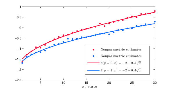
Figure 1. Comparison between the estimated and true utility flows.

5.2. Finite sample performance

To test the performance of our estimation procedure when there is sampling error in the CCPs, we generate simulated panel data of the following form: $\{y_{it}\;,x_{it}:i=1,2,\dots,N;\;t=1,2,\dots,T\}$ where $y_{it}\in\{0,1,2\}$ is the dynamically optimal choice at $x_{it}$ after the realization of simulated shocks. We vary the number of cross-section observations $N$ and the number periods $T$, and for each combination of $(N,T)$, we generate 100 independent datasets.

For each replication or simulated dataset, the root-mean-square error (RMSE) and $R^{2}$ are calculated, showing how well the estimated $\bar{u}_{y}(x)$ fits the true utility function for each $y$. The averages are reported in Table 1.

Design	RMSE($y=0$)	RMSE($y=1$)	$R^{2}(y=0)$	$R^{2}(y=1)$
$N=100,T=100$	0.5586	0.2435	0.3438	0.7708
$N=100,T=500$	0.1070	0.1389	0.7212	0.9119
$N=100,T=1000$	0.0810	0.1090	0.8553	0.9501
$N=200,T=100$	0.1244	0.1642	0.5773	0.8736
$N=200,T=200$	0.1177	0.1500	0.7044	0.9040
$N=500,T=100$	0.0871	0.1162	0.8109	0.9348
$N=500,T=500$	0.0665	0.0829	0.8899	0.9678
$N=1000,T=100$	0.0718	0.0928	0.8777	0.9647
$N=1000,T=1000$	0.0543	0.0643	0.9322	0.9820

Table 1. Average fit across all replications. Standard deviations are reported in the Appendix.

5.3. Size of the identified set of payoffs

As mentioned in Section 4.3, using a discrete approximation to the distribution of the unobserved state variable introduces a partial identification problem: the identified choice-specific value functions might not be unique. Using simulations, we next show that the identified set of choice-specific value functions (which we will simply refer to as “payoffs”) shrinks to a singleton as $S$ increases, where $S$ is the number of support points in the discrete approximation of the continuous error distribution. For $S$ ranging from 100 to 1000, we plot in Figure 2, the differences between the largest and smallest choice-specific value function for $y=2$ across all values of $p\in\Delta^{3}$ (using the linear programming procedures described in Section 4.3).

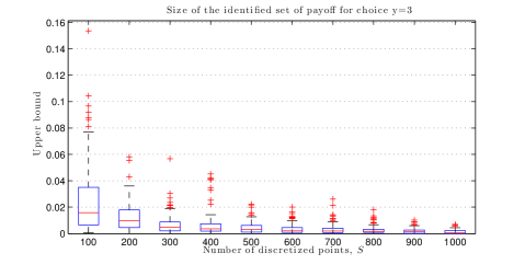
Figure 2. The identified set of payoffs shrinks to a singleton across $\Delta^{3}$.

For each value of $S$, we plot the values of the differences $\max_{w\in\partial\mathcal{G}^{*}(p)}w-\min_{w\in\partial\mathcal{G}^{*}(p)}w$ across all values of $p\in\Delta^{3}$. In the boxplot, the central mark is the median, the edges of the box are the 25th and 75th percentiles, the whiskers extend to the most extreme data points not considered outliers, and outliers are plotted individually.

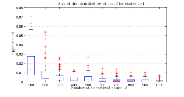
Figure 5. For each value of $S$, we plot the values of the differences $\max_{w\in\partial\mathcal{G}^{*}(p)}w_{1}-\min_{w\in\partial\mathcal{G}^{*}(p)}w_{1}$ across all values of $p\in\Delta^{3}$. In the boxplot, the central mark is the median, the edges of the box are the 25th and 75th percentiles, the whiskers extend to the most extreme data points not considered outliers, and outliers are plotted individually.

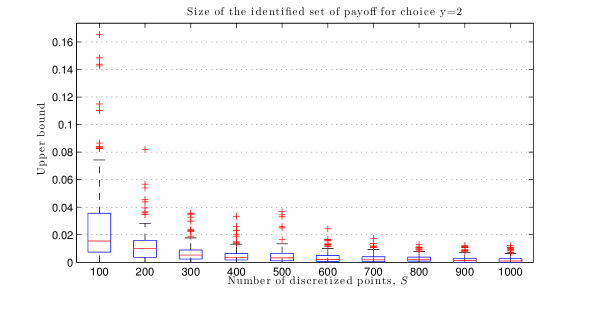
Figure 6. For each value of $S$, we plot the values of the differences $\max_{w\in\partial\mathcal{G}^{*}(p)}w_{2}-\min_{w\in\partial\mathcal{G}^{*}(p)}w_{2}$ across all values of $p\in\Delta^{3}$. In the boxplot, the central mark is the median, the edges of the box are the 25th and 75th percentiles, the whiskers extend to the most extreme data points not considered outliers, and outliers are plotted individually.

As is evident, even at small $S$, the identified payoffs are very close to each other in magnitude. At $S=1000$, where computation is near-instantaneous, for most of the values in the discretised grid of $\Delta^{3}$, the core is a singleton; when it is not, the difference in the estimated payoff is less than 0.01. Similar results hold for the choice-specific value functions for choices $y=0$ and $y=1$, which are plotted in Figures 5 and 6 in the Appendix. To sum up, it appears that this indeterminacy issue in the payoffs is not a worrisome problem for even very modest values of $S$.

5.4. Comparison: MTA vs. Simulated Maximum Likelihood

One common technique used in the literature to estimate dynamic discrete choice models with non-standard distribution of unobservables is the Simulated Maximum Likelihood (SML). Our MTA method has a distinct advantage over SML – while MTA allows the utility flows $\bar{u}_{y}(x)$ for different choices $y$ and states $x$ to be nonparametric, the SML approach typically requires parameterizing these utility flows as a function of a low-dimensional parameter vector. This makes comparison of these two approaches awkward. Nevertheless, here we undertake a comparison of the nonparametric MTA vs. the parametric SML approach. First we compare the performance of the two alternative approaches in terms of computational time. The computations were performed on a Quad Core Intel Xeon 2.93GHz UNIX workstation, and the results are presented in Table 2.

From a computational point of view, the disadvantage of SML is that the dynamic programming problem must be solved (via Bellman function iteration) for each trial parameter vector, whereas the MTA requires solving a large-scale linear programming problem – but only once. Table 2 shows that our MTA procedure significantly outperforms SML in terms of computational speed. This finding, along with the results in Table 1, show that MTA has the desirable properties of speed and accuracy, and also allows for nonparametric specification of the utility flows $\bar{u}_{y}(x)$.

Table 2. Comparison: MTA vs. Simulated Maximum Likelihood (SML)

$S$ discretized points	SML:+	MTA:++
	Avg. seconds	Avg. seconds
2000	19.8	2.6
3000	24.5	4.4
4000	26.5	6.6
5000	40.9	9.6
6000	70.5	13.4
7000	105.0	17.5
8000	129.4	21.5

⁺:In this column we report time it takes to estimate the parameters $\theta=(\theta_{00},\theta_{01},\theta_{10},\theta_{11})$ as a local maximum of a simulated maximum likelihood, where $\theta$ corresponds to $\bar{u}_{y=0}(x)=\theta_{00}+\theta_{01}\sqrt{x}$, and $\bar{u}_{y=1}(x)=\theta_{10}+\theta_{11}\sqrt{x}$.
⁺⁺:In this column we report the time it takes to nonparametrically estimate the per-period utility flow.

Furthermore, as confirmed in our computations, the nonlinear optimization routines typically used to implement SML have trouble finding the global optimum; in contrast, the MTA estimator, by virtue of its being a linear programming problem, always finds the global optimum. Indeed, under the logistic assumption on unobservables and linear-in-parameters utility, one advantage of the Hotz-Miller estimator for DDC models (vs. SML) is that the system of equations defining the estimator has a unique global solution; in their discussion of this, Aguirregabiria and Mira (2010, pg. 48) remark that “extending the range of applicability of … CCP methods to models which do not impose the CLOGIT [logistic] assumption is a topic for further research.” This paper fills the gap: our MTA estimator shares the computational advantages of the CLOGIT setup, but works for non-logistic models. In this sense, the MTA estimator is a generalized CCP estimator.

6. Empirical Application: Revisiting Harold Zurcher

In this section, we apply our estimation procedure to the bus engine replacement dataset first analyzed in Rust (1987). In each week $t$, Harold Zurcher (bus depot manager), chooses $y_{t}\in\{0,1\}$ after observing the mileage $x_{t}\in\mathcal{X}$ and the realized shocks $\varepsilon_{t}$. If $y_{t}=0$, then he chooses not to replace the bus engine, and $y_{t}=1$ means that he chooses to replace the bus engine. The states space is $\mathcal{X}=\{0,1,\dots 29\}$, that is, we divided the mileage space into 30 states, each representing a 12,500 increment in mileage since the last engine replacement. Harold Zurcher manages a fleet of 104 identical buses, and we observe the decisions that he made, as well as the corresponding bus mileage at each time period $t$. The duration between $t+1$ and $t$ is a quarter of a year, and the dataset spans 10 years. Figures 7 and 8 in the Appendix summarize the frequencies and mileage at which replacements take place in the dataset.

Firstly, we can directly estimate the probability of choosing to replace and not to replace the engine for each state in $\mathcal{X}$. Also directly obtained from the data is the Markov transition probabilities for the observed state variable $x_{t}\in X$, estimated as:

$$\hat{\text{Pr}}(x_{t+1}=j|x_{t}=i,y_{t}=0)=\begin{cases}0.7405&\mbox{if}\quad j=i\\ 0.2595&\mbox{if}\quad j=i+1\\ 0&\mbox{otherwise}\end{cases}$$

$$\hat{\text{Pr}}(x_{t+1}=j|x_{t}=i,y_{t}=1)=\begin{cases}0.7405&\mbox{if}\quad j=0\\ 0.2595&\mbox{if}\quad j=1\\ 0&\mbox{otherwise}\end{cases}$$

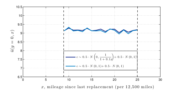
Figure 3. Estimates of utility flows $\bar{u}_{y=0}(x)$, across values of mileage $x$

For this analysis, we assumed a normal mixture distribution of the error term, specifically, $\varepsilon_{t0}-\varepsilon_{t1}\sim\frac{1}{2}N(0,1)+\frac{1}{2}N(0,\frac{1}{1+0.1x})$. We chose this mixture distribution in order to allow the utility shocks to depend on mileage – which accommodates, for instance, operating costs which may be more volatile and unpredictable at different levels of mileage. At the same time, these specifications for the utility shock distribution showcase the flexibility of our procedure in estimating dynamic discrete choice models for any general error distribution. For comparison, we repeat this exercise using an error distribution that is homoskedastic, i.e., its variance does not depend on the state variable $x_{t}$. The result appears to be robust to using different distributions of $\varepsilon_{t0}-\varepsilon_{t1}$. We set the discount rate $\beta=0.9$.

To non-parametrically estimate $\bar{u}_{y=0}(x)$, we fixed $\bar{u}_{y=1}(x)$ to 0 for all $x\in X$. Hence, our estimates of $\bar{u}_{y=0}(x)$ should be interpreted as the magnitude of operating costs relative to replacement costs, with positive values implying that replacement costs exceed operating costs. The estimated utility flows from choosing $y=0$ (don’t replace) relative to $y=1$ (replace engine) are plotted in Figure 3. We only present estimates for mileage within the range $x\in[9,25]$, because within this range, the CCPs are in the interior of the probability simplex (cf. footnote 28 and Figure 8 in appendix).

Within this range, the estimated utility function does not vary much with increasing mileages, i.e. it has slope that is not significantly different from zero. The recovered utilities fall within the narrow band of 9 and 9.5, which implies that on average the replacement cost is much higher than the maintenance cost, by a magnitude of 18 to 19 times the variance of the utility shocks. It is somewhat surprising that our results suggest that when the mileage goes beyond the cutoff point of 100,000 miles, Harold Zurcher perceived the operating costs to be inelastic with respect to accumulated mileage. It is worth noting that Rust (1987) mentioned: “According to Zurcher, monthly maintenance costs increase very slowly as a function of accumulated mileage.”

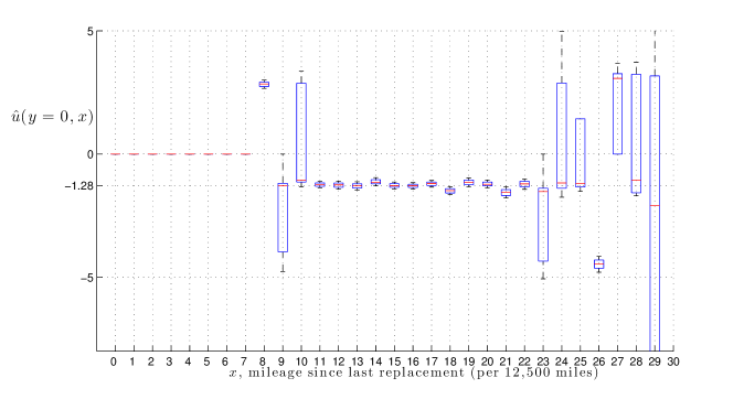
Figure 4. Bootstrapped estimates of utility flows $\bar{u}_{y=0}(x)$

We plot the values of the bootstrapped resampled estimates of $\bar{u}_{y=0}(x)$. In each boxplot, the central mark is the median, the edges of the box are the 25th and 75th percentiles, the whiskers extend to the 5th and 95th percentiles.

To get an idea for the effect of sampling error on our estimates, we bootstrapped our estimation procedure. For each of 100 resamples, we randomly drew 80 buses with replacement from the dataset, and re-estimated the utility flows $\bar{u}_{y=0}(x)$ using our procedure. The results are plotted in Figure 4. The evidence suggests that we are able to obtain fairly tight cost estimates for states where there is at least one replacement, i.e. for $x\geq 9$ ($x\geq 112,500$ miles), and for states that are reached often enough; i.e. for $x\leq 22$ ($x\leq 275,000$ miles).

7. Conclusion

In this paper, we have shown how results from convex analysis can be fruitfully applied to study identification in dynamic discrete choice models; modulo the use of these tools, a large class of dynamic discrete choice problems with quite general utility shocks becomes no more difficult to compute and estimate than the Logit model encountered in most empirical applications. This has allowed us to provide a natural and holistic framework encompassing the papers of Rust (1987), Hotz and Miller (1993), and Magnac and Thesmar (2002). While the identification results in this paper are comparable to other results in the literature, the approach we take, based on the convexity of the social surplus function $\mathcal{G}$ and the resulting duality between choice probabilities and choice-specific value functions, appears new. Far more than providing a mere reformulation, this approach is powerful, and has significant implications in several dimensions.

First, by drawing the (surprising) connection between the computation of the $\mathcal{G}^{\ast}$ function and the computation of optimal matchings in the classical assignment game, we can apply the powerful tools developed to compute optimal matchings to dynamic discrete-choice models. Moreover, by reformulating the problem as an optimal matching problem, all existence and uniqueness results are inherited from the theory of optimal transport. For instance, the uniqueness of a systematic utility rationalizing the consumer’s choices follows from the uniqueness of a potential in the Monge-Kantorovich theorem.

We believe the present paper opens a more flexible way to deal with discrete choice models. While identification is exact for a fixed structure of the unobserved heterogeneity, one may wish to parameterize the distribution of the utility shocks and do inference on that parameter. The results and methods developed in this paper may also extend to dynamic discrete games, with the utility shocks reinterpreted as players’ private information. However, we leave these directions for future exploration.

Appendix A Background results

A.1. Convex Analysis for Discrete-choice Models

Here, we give a brief review of the main notions and results used in the paper. We keep an informal style and do not give proofs, but we refer to Rockafellar (1970) for an extensive treatment of the subject.

Let $u\in\mathbb{R}^{|\mathcal{Y}|}$ be a vector of utility indices. For utility shocks $\{\varepsilon_{y}\}_{y\in\mathcal{Y}}$ distributed according to a joint distribution function $Q$, we define the social surplus function as

$$\mathcal{G}(u)={\mathbb{E}}[\max_{y}{\{u_{y}+\varepsilon_{y}}\}],$$ (23)

where $u_{y}$ is the $y$-th component of $u$. If ${\mathbb{E}}(\varepsilon_{y})$ exists and is finite, then the function $\mathcal{G}$ is a proper convex function that is continuous everywhere. Moreover assuming that $Q$ is sufficiently well-behaved (for instance, if it has a density with respect to the Lebesgue measure), $\mathcal{G}$ is differentiable everywhere.

Define the Legendre-Fenchel conjugate, or convex conjugate of $\mathcal{G}$ as $\mathcal{G}^{\ast}(p)=\sup_{u\in\mathbb{R}^{|\mathcal{Y}|}}\{p\cdot u-\mathcal{G}(u)\}$. Clearly, $\mathcal{G}^{\ast}$ is a convex function as it is the supremum of affine functions. Note that the inequality

$$\mathcal{G}(u)+\mathcal{G}^{\ast}(p)\geq p\cdot u$$ (24)

holds in general. The domain of $\mathcal{G}^{\ast}$ consists of $p\in\mathbb{R}^{|\mathcal{Y}|}$ for which the supremum is finite. In the case when $\mathcal{G}$ is defined by (23), it follows from Norets and Takahashi (2013) that the domain of $\mathcal{G}^{\ast}$ contains the simplex $\Delta^{|\mathcal{Y}|}$, which is the set of $p\in\mathbb{R}^{|\mathcal{Y}|}$ such that $p_{y}\geq 0$ and $\sum_{y\in\mathcal{Y}}p_{y}=1$. This means that our convex conjugate function is always well-defined.

The subgradient $\partial\mathcal{G}\left(u\right)$ of $\mathcal{G}$ at $u$ is the set of $p\in\mathbb{R}^{|\mathcal{Y}|}$ such that

$$p\cdot u-\mathcal{G}(u)\geq p\cdot u^{\prime}-\mathcal{G}(u^{\prime})$$

holds for all $u^{\prime}\in\mathbb{R}^{|\mathcal{Y}|}$. Hence $\partial\mathcal{G}$ is a set-valued function or correspondence. $\partial\mathcal{G}\left(u\right)$ is a singleton if and only if $\mathcal{G}(u)$ is differentiable at $u$; in this case, $\partial\mathcal{G}\left(u\right)=\nabla\mathcal{G}\left(u\right)$.

One sees that $p\in\partial\mathcal{G}\left(u\right)$ if and only if $p\cdot u-\mathcal{G}(u)=\mathcal{G}^{\ast}(p)$, that is if equality is reached in inequality (24):

$$\mathcal{G}(u)+\mathcal{G}^{\ast}(p)=p\cdot u.$$ (25)

This equation is itself of interest, and is known in the literature as “Fenchel’s equality”. By symmetry in (25), one sees that $p\in\partial\mathcal{G}\left(u\right)$ if and only if $u\in\partial\mathcal{G}^{\ast}(p)$. In particular, when both $\mathcal{G}$ and $\mathcal{G}^{\ast}$ are differentiable, then $\nabla\mathcal{G}^{\ast}=\nabla\mathcal{G}^{-1}$.

Appendix B Proofs

Proof of Proposition 1.

Consider the $y$-th component, corresponding to $\frac{\partial\mathcal{G}(w)}{\partial w_{y}}$:

$$\frac{\partial\mathcal{G}(w)}{\partial w_{y}} =\frac{\partial}{\partial w_{y}}\int\max_{y}[w_{y}+\varepsilon_{y}]dQ$$ (26)

$$=\int\frac{\partial}{\partial w_{y}}\max_{y}[w_{y}+\varepsilon_{y}]dQ$$ (27)

$$=\int\mathbbm{1}(w_{y}+\varepsilon_{y}\geq w_{y^{\prime}}+\varepsilon_{y^{\prime}}),\forall y^{\prime}\neq y)dQ=p(y).$$ (28)

(We have suppressed the dependence on $x$ for convenience.)    

Proof of Theorem 1.

This follows directly from Fenchel’s equality (see Rockafellar (1970), Theorem 23.5, see also Appendix A.1), which states that

$$p\in\partial\mathcal{G}\left(w\right)$$

is equivalent to $\mathcal{G}\left(w\right)+\mathcal{G}^{\ast}\left(p\right)=\sum_{y}p_{y}w_{y}$, which is equivalent in turn to

$$w\in\partial\mathcal{G}^{\ast}\left(p\right).$$

   

Proof of Theorem 2.

Because $\varepsilon$ has full support, the choice probabilities $p$ will lie strictly in the interior of the simplex $\Delta^{|\mathcal{Y}|}$. Let $\tilde{w}\in\partial\mathcal{G}^{\ast}\left(p\right)$, and let $w_{y}=\tilde{w}_{y}-\mathcal{G}\left(\tilde{w}\right)$. One has $\mathcal{G}\left(w\right)=0$, and an immediate calculation shows that $\partial\mathcal{G}\left(w\right)=p$. Let us now show that $w$ is unique. Consider $w$ and $w^{\prime}$ such that $\mathcal{G}\left(w\right)=\mathcal{G}\left(w^{\prime}\right)=0$, and $p\in\partial\mathcal{G}\left(w\right)$ and $p\in\partial\mathcal{G}\left(w^{\prime}\right)$. Assume $w\neq w^{\prime}$ to get a contradiction; then there exist two distinct $y_{0}$ and $y_{1}$ such that $w_{y_{0}}-w_{y_{1}}\neq w_{y_{0}}^{\prime}-w_{y_{1}}^{\prime}$; without loss of generality one may assume

$$w_{y_{0}}-w_{y_{1}}>w_{y_{0}}^{\prime}-w_{y_{1}}^{\prime}.$$

Let $S$ be the set of $\varepsilon$’s such that

$$w_{y_{0}}-w_{y_{1}}>\varepsilon_{y_{1}}-\varepsilon_{y_{0}}>w_{y_{0}}^{\prime}-w_{y_{1}}^{\prime}$$

$$w_{y_{0}}+\varepsilon_{y_{0}}>\max_{y\neq y_{0},y_{1}}\left\{w_{y}+\varepsilon_{y}\right\}$$

$$w_{y_{1}}^{\prime}+\varepsilon_{y_{1}}>\max_{y\neq y_{0},y_{1}}\left\{w_{y}^{\prime}+\varepsilon_{y}\right\}$$

Because $\varepsilon$ has full support, $S$ has positive probability.

Let $\bar{w}=\frac{w+w^{\prime}}{2}$. Because $p\in\partial\mathcal{G}\left(w\right)$ and $p\in\partial\mathcal{G}\left(w^{\prime}\right)$, $\mathcal{G}$ is linear on the segment $\left[w,w^{\prime}\right]$, thus  $\mathcal{G}\left(\bar{w}\right)=0$, thus

$$0 = \mathbb{E}\left[\bar{w}_{Y\left(\bar{w},\varepsilon\right)}+\varepsilon_{Y\left(\bar{w},\varepsilon\right)}\right]=\frac{1}{2}\mathbb{E}\left[w_{Y\left(\bar{w},\varepsilon\right)}+\varepsilon_{Y\left(\bar{w},\varepsilon\right)}\right]+\frac{1}{2}\mathbb{E}\left[w_{Y\left(\bar{w},\varepsilon\right)}^{\prime}+\varepsilon_{Y\left(\bar{w},\varepsilon\right)}\right]$$

$$\leq \frac{1}{2}\mathbb{E}\left[w_{Y\left(w,\varepsilon\right)}+\varepsilon_{Y\left(w,\varepsilon\right)}\right]+\frac{1}{2}\mathbb{E}\left[w_{Y\left(w^{\prime},\varepsilon\right)}^{\prime}+\varepsilon_{Y\left(w^{\prime},\varepsilon\right)}\right]$$

$$= \frac{1}{2}\left(\mathcal{G}\left(w\right)+\mathcal{G}\left(w^{\prime}\right)\right)=0$$

Hence equality holds term by term, and

$$w_{Y\left(w,\varepsilon\right)}+\varepsilon_{Y\left(w,\varepsilon\right)} = w_{Y\left(\bar{w},\varepsilon\right)}+\varepsilon_{Y\left(\bar{w},\varepsilon\right)}$$

$$w_{Y\left(w^{\prime},\varepsilon\right)}^{\prime}+\varepsilon_{Y\left(w^{\prime},\varepsilon\right)} = w_{Y\left(\bar{w},\varepsilon\right)}^{\prime}+\varepsilon_{Y\left(\bar{w},\varepsilon\right)}$$

For $\varepsilon\in S$, $Y\left(w,\varepsilon\right)=Y\left(\bar{w},\varepsilon\right)=y_{0}$ and $Y\left(w^{\prime},\varepsilon\right)=Y\left(\bar{w},\varepsilon\right)=y_{1}$, and we get the desired contradiction.

Hence $w=w^{\prime}$, and the uniqueness of $w$ follows.    

Proof of Theorem 3.

From $\mathcal{G}\left(w^{0}\right)=0$ and $\partial\mathcal{G}\left(w-\mathcal{G}\left(w\right)\right)=\partial\mathcal{G}\left(w\right)$, and by the uniqueness result in Theorem 2, it follows that

$$w^{0}=w-\mathcal{G}\left(w\right).$$

   

Proof of Proposition 2.

The proof is in Galichon and Salanié (2012), but we include it here for self-containedness. This connection between the $\mathcal{G}^{\ast}$ function and a matching model follows from manipulation of the variational problem in the definition of $\mathcal{G}^{\ast}$:

$$\mathcal{G}^{\ast}\left(p\right) = \sup_{w\in\mathbb{R}^{\mathcal{Y}}}\left\{\sum_{y}p_{y}w_{y}-\mathbb{E}_{Q}\left[\max_{y\in\mathcal{Y}}\left(w_{y}+\varepsilon_{y}\right)\right]\right\}$$

$$= \sup_{w\in\mathbb{R}^{\mathcal{Y}}}\left\{\sum_{y}p_{y}w_{y}+\mathbb{E}_{Q}\underset{\equiv z(\varepsilon)}{\underbrace{\left[\min_{y\in\mathcal{Y}}\left(-w_{y}-\varepsilon_{y}\right)\right]}}\right\}.$$

Defining $c\left(y,\varepsilon\right)\equiv-\varepsilon_{y}$, one can rewrite the above as

$$\mathcal{G}^{\ast}\left(p\right)=\sup_{w_{y}+z\left(\varepsilon\right)\leq c\left(y,\varepsilon\right)}\left\{\mathbb{E}_{p}\left[w_{Y}\right]+\mathbb{E}_{Q}\left[z\left(\varepsilon\right)\right]\right\}.$$ (30)

As is well-known from the results of Monge-Kantorovich (Villani (2003), Thm. 1.3), this is the dual-problem for a mass transport problem. The corresponding primal problem is

$$\mathcal{G}^{\ast}\left(p\right)=\min_{\begin{subarray}{c}Y\sim p\\ \varepsilon\sim\hat{Q}\end{subarray}}\mathbb{E}\left[c\left(Y,\varepsilon\right)\right]$$

which is equivalent to (16)-(18). Comparing Eqs. (B) and (30), we see that the subdifferential $\partial{\mathcal{G}}^{\ast}(p)$ is identified with those elements $w$ such that $(w,z)$, for some $z$, solves the dual problem (30).    

Proof of Theorem 4.

(i) follows from Proposition 2 and the fact that if $w_{y}+z\left(\varepsilon\right)\leq c\left(y,\varepsilon\right)$, then $\mathbb{E}_{p}\left[w_{Y}\right]+\mathbb{E}_{Q}\left[z\left(\varepsilon\right)\right]=\mathcal{G}^{\ast}\left(p\right)$ if and only if $\left(w,z\right)$ is a solution to the dual problem.

(ii) follows from the fact that $-z\left(\varepsilon\right)=\sup_{y}\left\{w_{y}-c\left(y,\varepsilon\right)\right\}=\sup_{y}\left\{w_{y}+\varepsilon_{y}\right\}$, thus $\mathbb{E}_{Q}\left[z\left(\varepsilon\right)\right]=0$ is equivalent to $\mathbb{E}_{Q}\left[\sup_{y}\left\{w_{y}+\varepsilon_{y}\right\}\right]=0$, that is $\mathcal{G}\left(w\right)=0$.    

Proof of Theorem 5.

We shall show that the vector of choice-specific value functions derived from the MTA estimation procedure, denoted $w^{n}$, converges to the true vector $w^{0}$. In our procedure, there are two sources of estimation error. The first is the sampling error in the vector of choice probabilities, denoted ${p}^{n}$. The second is the simulation error involved in the discretization of the distribution of $\varepsilon$; we let $Q^{n}$ denote this discretized distribution.

A distinctive aspect of our proof is that it utilizes the theory of mass transport; namely convergence results for sequences of mass transport problems. For $y\in\mathcal{Y}$, let $\iota^{y}$ denote the $|\mathcal{Y}|$-dimensional row vector with all zeros except a 1 in the $y$-th column. This discretized mass transport problem from which we obtain $w^{n}$ is:

$$\sup_{\gamma\in\mathcal{M}(Q^{n},{p}^{n})}\int_{{\mathbb{R}}^{d}\times{\mathbb{R}}^{d}}\left(\iota\cdot\varepsilon\right)\gamma(d\varepsilon,d\iota)$$ (31)

where $\mathcal{M}(Q^{n},{p}^{n})$ denotes the set of joint (discrete) probability measures with marginal distributions $Q^{n}$ and $p^{n}$. In the above, $\iota$ denotes a random vector which is equal to $\iota^{y}$ with probability $p_{y}^{n}$, for $y\in\mathcal{Y}$. The dual problem used in the MTA procedure is

$$\inf_{z,w} \int z\left(\varepsilon\right)dQ^{n}\left(\varepsilon\right)+\sum_{y}w_{y}p_{y}^{n}\;:$$ (32)

$$s.t.~{} z(\varepsilon)\geq\iota^{y}\cdot\varepsilon-w_{y},\;\forall y,\;\forall\varepsilon$$ (34)

$$\mathcal{G}_{n}(w_{y}^{n})=0,$$

where $\mathcal{G}_{n}(w)\equiv\mathbb{E}_{Q^{n}}(w_{y}+\epsilon_{y})$. We let $(z^{n},w^{n})$ denote solutions to this discretized dual problem $(\ref{dual1})$. Recall (from the discussion in Section 2.3) that the extra constraint (34) in the dual problem just selects among the many dual optimizing arguments $(w^{n},z^{n})$ corresponding to the optimal primal solution $\gamma^{n}$, and so does not affect the primal problem.

Next we derive a more manageable representation of this constraint (34). From Fenchel’s Equality (Eq. (25)), we have $\sum_{y}p_{y}^{n}w_{y}^{n}=\mathcal{G}_{n}(w^{n})+\mathcal{G}^{*}_{n}(p^{n})=\mathcal{G}_{n}^{\ast}(p^{n})$ (with $\mathcal{G}_{n}^{\ast}$ defined as the convex conjugate function of $\mathcal{G}_{n}$). Moreover, from Proposition 2, we know that $\mathcal{G}_{n}^{\ast}(p^{n})$ can be characterized as the optimized dual objective function in (32). Hence, we see that the constraint $\mathcal{G}_{n}(w^{n})=0$ is equivalent to $\int z^{n}(\varepsilon)dQ^{n}(\varepsilon)=0$. We introduce this latter constraint directly and rewrite the dual program

$$\inf_{z,w} \sum_{y}w_{y}p_{y}^{n}+\int z\left(\varepsilon\right)dQ^{n}\left(\varepsilon\right)$$ (35)

$$s.t.~{} z(\varepsilon)\geq\iota^{y}\cdot\varepsilon-w_{y},\;\forall y,\;\forall\varepsilon$$ (37)

$$\int z\left(\varepsilon\right)dQ^{n}\left(\varepsilon\right)=0.$$

We will demonstrate consistency by showing that $(z^{n},w^{n})$ converge a.s. to the dual optimizers in the “limit” dual problem, given by

$$\inf_{z,w} \sum_{y}w_{y}p_{y}^{0}$$ (40)

$$z(\varepsilon)\geq\iota^{y}\cdot\varepsilon-w_{y},\;\forall y,\;\forall\varepsilon$$

$$\int z\left(\varepsilon\right)dQ=0$$

We denote the optimizers in this limit problem by $(w^{0},z^{0})$, where, by construction, $w^{0}$ are the “true” values of the choice-specific value functions. The difference between the discretized and limit dual problems is that $Q^{n}$ in the former has been replaced by $Q$, the continuous distribution of $\varepsilon$, and the estimated choice probabilities $p^{n}$ have been replaced by the limit $p^{0}$.

We proceed in two steps. First, we argue that the sequence of optimized dual programs (35) converges to the optimized limit dual program (40), a.s. Based upon this, we then argue that the sequence of dual optimizers, $(w^{n},z^{n})$, necessarily converge to their unique limit optimizers, $(w^{0},z^{0})$, a.s.

First step. By the Kantorovich duality theorem, we know that the optimized values for the limit primal and dual programs coincide

$$\sup_{\gamma\in\Pi(Q^{0},p^{0})}\int_{{\mathbb{R}}^{d}\times{\mathbb{R}}^{d}}\left(\iota\cdot\varepsilon\right)\gamma(d\varepsilon,d\iota)=\inf\sum_{y}w_{y}p_{y}^{0}+\int z\left(\varepsilon\right)dQ.$$ (41)

Moreover, both the primal and dual problems in the discretized case are finite-dimensional linear programming problem, and by the usual LP duality, the optimal primal and dual problems for the discretized case also coincide:

$$\int_{{\mathbb{R}}^{d}\times{\mathbb{R}}^{d}}\left(\iota\cdot\varepsilon\right)\gamma_{n}(d\varepsilon,d\iota)=\sum_{y}w_{y}^{n}p_{y}^{n}+\int z^{n}\left(\varepsilon\right)dQ^{n}.$$

Given Assumption 1, and by Theorem 5.20 in Villani (2009), p. 77, we have that, up to a subsequence extraction, $\gamma^{n}$ (the optimizing argument of (31)) converges weakly. In addition, by Theorem 5.30 in Villani (2009), the left-hand side of (41) has a unique solution $\gamma$; hence, the sequence $\gamma^{n}$ must converge generally to $\gamma$. This implies a.s. convergence of the value of the primal problems:

$$\int_{{\mathbb{R}}^{d}\times{\mathbb{R}}^{d}}\left(\iota\cdot\varepsilon\right)\gamma_{n}(d\varepsilon,d\iota)\rightarrow\int_{{\mathbb{R}}^{d}\times{\mathbb{R}}^{d}}\left(\iota\cdot\varepsilon\right)\gamma(d\varepsilon,d\iota),\quad a.s.,$$

and, by duality, we must also have a.s. convergence of the discretized dual problem to the limit problem:

$$\sum_{y}w_{y}^{n}p_{y}^{n}+\int z^{n}\left(\varepsilon\right)dQ^{n}\rightarrow\sum_{y}w_{y}p_{y}^{0}+\int z\left(\varepsilon\right)dQ,\quad a.s.$$ (42)

Second step. Next, we show that the discretized dual minimizers $(z^{n},w^{n})$ converge a.s. For convenience, in what follows we will suppress the qualifier “a.s.” from all the statements below. Let

$$\text{\@text@baccent{w}}^{n}=\min_{y}w_{y}^{n}.$$ (43)

From examination of the dual problem (35), we see that $z^{n}$ is the piecewise affine function

$$z^{n}(\varepsilon)=\max_{y}\{\iota^{y}\cdot\varepsilon-w_{y}^{n}\},$$ (44)

thus $z^{n}$ is $M$-Lipschitz with $M:=\max_{y}|\iota^{y}|=1$. Now observe that

$$z^{n}(\varepsilon)+\text{\@text@baccent{w}}^{n}=\max_{y}\{\iota^{y}\cdot\varepsilon-w_{y}^{n}+\text{\@text@baccent{w}}^{n}\}\leq\max_{y}\{\iota^{y}\cdot\varepsilon\}=:\overline{z}(\varepsilon)$$ (45)

and, letting $y^{\prime}$ be the argument of the minimum in (43),

$$z^{n}(\varepsilon)+\text{\@text@baccent{w}}^{n}\geq\iota^{y^{\prime}}\cdot\varepsilon-w_{y^{\prime}}^{n}+\text{\@text@baccent{w}}^{n}=\iota^{y^{\prime}}\cdot\varepsilon\geq\min_{y}\{\iota^{y}\cdot\varepsilon\}=:\underline{z}(\varepsilon)$$ (46)

thus, by a combination of (45) and (46),

$$\underline{z}(\varepsilon)\leq z^{n}(\varepsilon)+\text{\@text@baccent{w}}^{n}\leq\overline{z}(\varepsilon).$$ (47)

By $\int z^{n}\left(\varepsilon\right)dQ^{n}\left(\varepsilon\right)=0$, we have that that w̱ⁿ is uniformly bounded (sublinear): for some constant $K$, $|z^{n}(\varepsilon)|\leq C(1+|\varepsilon|)$ for every $n$ and every $\varepsilon$. Hence the sequence $z^{n}$ is uniformly equicontinuous, and converges locally uniformly up to a subsequence extraction by Ascoli’s theorem. Let this limit function be denoted $z^{0}$. By (42), and Theorem 2, we deduce that $z$, the optimizer in the limit dual problem is unique, so that it must coincide with the limit function $z^{0}$.

By the definition of $(w^{n},z^{n})$ as optimizing arguments for (35), we have $\sum_{y}w_{y}^{n}p_{y}^{n}\leq\sum_{y}\text{\@text@baccent{w}}^{n}p_{y}+\int[\overline{z}\left(\varepsilon\right)]dQ^{n}\left(\varepsilon\right)$ or

$$\sum_{y}\left(w_{y}^{n}-\text{\@text@baccent{w}}^{n}\right)p_{y}^{n}\leq\int[\overline{z}\left(\varepsilon\right)]dQ^{n}\left(\varepsilon\right)=\mathbb{E}_{Q^{n}}\overline{z}$$

The second moment restrictions on $Q^{n}$ (condition (ii) in the theorem) imply that $\mathbb{E}_{Q^{n}}\overline{z}(\varepsilon)$ exists and converges to $\mathbb{E}_{Q}\overline{z}$. Hence, the nonnegative vectors $\left(w_{y}^{n}-\text{\@text@baccent{w}}^{n}\right)$ are bounded; accordingly, the vectors $\left(w_{y}^{n}\right)$ are themselves bounded. This implies that $w^{n}$ converges up to a subsequence to some limit point $w^{\ast}$, using the Bolzano-Weierstrass theorem. This implies that $\sum_{y}w_{y}^{n}p_{y}^{n}\rightarrow\sum_{y}w_{y}^{\ast}p_{y}$ by bounded convergence. By Theorem 2, we know that the limit point $w^{\ast}$ must coincide with $w^{0}$, which is the unique optimizer in the dual limit problem (40). Thus, we have shown that $w^{n}$ converges to $w^{0}$, a.s.    

Appendix C Additional Figures

Design	RMSE($y=0$)	RMSE($y=1$)	$R^{2}(y=0)$	$R^{2}(y=1)$
$N=100,T=100$	0.5586 (3.7134)	0.2435 (0.1155)	0.3438 (0.7298)	0.7708 (0.2073)
$N=100,T=500$	0.1070 (0.0541)	0.1389 (0.0638)	0.7212 (0.2788)	0.9119 (0.0820)
$N=100,T=1000$	0.0810 (0.0376)	0.1090 (0.0425)	0.8553 (0.1285)	0.9501 (0.0352)
$N=200,T=100$	0.1244 (0.0594)	0.1642 (0.0628)	0.5773 (0.6875)	0.8736 (0.1112)
$N=200,T=200$	0.1177 (0.0736)	0.1500 (0.0816)	0.7044 (0.2813)	0.9040 (0.0842)
$N=500,T=100$	0.0871 (0.0375)	0.1162 (0.0430)	0.8109 (0.2468)	0.9348 (0.0650)
$N=500,T=500$	0.0665 (0.0261)	0.0829 (0.0290)	0.8899 (0.1601)	0.9678 (0.0374)
$N=1000,T=100$	0.0718 (0.0340)	0.0928 (0.0344)	0.8777 (0.1320)	0.9647 (0.0314)
$N=1000,T=1000$	0.0543 (0.0176)	0.0643 (0.0162)	0.9322 (0.0577)	0.9820 (0.0101)

Table 3.

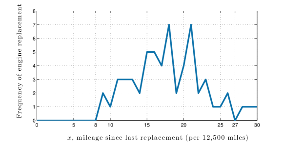
Figure 7.

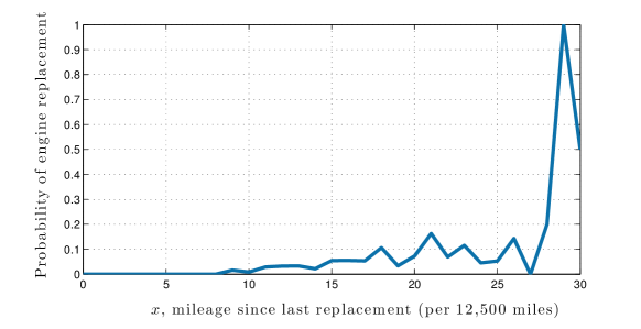
Figure 8.

References

- [1] V. Aguirregabiria and P. Mira. Swapping the nested fixed point algorithm: A class of estimators for discrete Markov decision models. Econometrica, 70:1519-1543, 2002.
- [2] V. Aguirregabiria and P. Mira. Sequential estimation of dynamic discrete games. Econometrica, 75:1–53, 2007.
- [3] V. Aguirregabiria and P. Mira. Dynamic discrete choice structural models: a survey. Journal of Econometrics, 156:38–67, 2010.
- [4] Anderson, S., de Palma, A., and Thisse, J.-F. A Representative Consumer Theory of the Logit Model. International Economic Review, 29(3), 461-466, 1988.
- [5] P. Arcidiacono and R. Miller. Conditional Choice Probability Estimation of Dynamic Discrete Choice Models with Unobserved Heterogeneity. Econometrica, 79: 1823-1867, 2011.
- [6] P. Arcidiacono and R. Miller. Identifying Dynamic Discrete Choice Models off Short Panels. Working paper, 2013.
- [7] C. Aliprantis and K. Border. Infinite Dimensional Analysis: A Hitchhiker’s Guide. Springer-Verlag, 2006.
- [8] P. Bajari, V. Chernozhukov, H. Hong, and D. Nekipelov. Nonparametric and semiparametric analysis of a dynamic game model. Preprint, 2009.
- [9] S. Berry, A. Gandhi, and P. Haile. Connected Substitutes and Invertibility of Demand. Econometrica 81: 2087-2111, 2013.
- [10] S. Berry. Estimating Discrete-Choice models of Production Differentiation. RAND Journal of Economics, 25:242-262, 1994.
- [11] S. Berry, J. Levinsohn, and A. Pakes. Automobile prices in market equilibrium. Econometrica, 63:841–890, July 1995.
- [12] D. Bertsekas. Dynamic Programming Deterministic and Stochastic Models. Prentice-Hall, 1987.
- [13] P. Chiappori and I. Komunjer. On the Nonparametric Identification of Multiple Choice Models. Working paper, 2010.
- [14] K. Chiong, A. Galichon, and M. Shum. Simulation and Partial Identification in Random Coefficient Discrete Choice Demand Models. Work in progress, 2014.
- [15] R. Cominetti, E. Melo, and S. Sorin. A payoff-based learning procedure and its application to traffic games. Games and Economic Behavior, 70:71-83, 2010.
- [16] A. Galichon and B. Salanié. Cupid’s invisible hand: Social surplus and identification in matching models. Preprint, 2012.
- [17] N. Gretsky, J. Ostroy, and W. Zame. Perfect Competition in the Continuous Assignment Model. Journal of Economic Theory, Vol. 85, pp. 60-118, 1999.
- [18] P. Haile, A. Hortacsu, and G. Kosenok. On the Empirical Content of Quantal Response Models. American Economic Review, 98:180-200, 2008.
- [19] J. Hofbauer and W. Sandholm. On the Global Convergence of Stochastic Fictitious Play. Econometrica, 70: 2265-2294, 2002.
- [20] J. Hotz and R. Miller. Conditional choice probabilties and the estimation of dynamic models. Review of Economic Studies, 60:497–529, 1993.
- [21] J. Hotz, R. Miller, S. Sanders, and J. Smith. A Simulation Estimator for Dynamic Models of Discrete Choice. Review of Economic Studies, 61:265-289, 1994.
- [22] Y. Hu and M. Shum. Nonparametric Identification of Dynamic Models with Unobserved Heterogeneity. Journal of Econometrics, 171: 32-44, 2012.
- [23] H. Kasahara and K. Shimotsu. Nonparametric Identification of Finite Mixture Models of Dynamic Discrete Choice. Econometrica, 77: 135–175, 2009.
- [24] M. Keane and K. Wolpin. The career decisions of young men. Journal of Political Economy, 105: 473–522, 1997.
- [25] J. Kennan. A Note on Discrete Approximations of Continuous Distributions. Mimeo, University of Wisconsin at Madison, 2006.
- [26] T. Magnac and D. Thesmar. Identifying dynamic discrete decision processes. Econometrica, 70:801–816, 2002.
- [27] D. McFadden. Modeling the choice of residential location. In A. Karlquist et. al., editor, Spatial Interaction Theory and Residential Location. North Holland Pub. Co., 1978.
- [28] D. McFadden. Economic Models of Probabilistic Choice. In C. Manski and D. McFadden, editors, Structural Analysis of Discrete Data with Econometric Applications, 1981.
- [29] A. Norets. Inference in dynamic discrete choice models with serially correlated unobserved state variables. Econometrica, 77: 1665-1682, 2009.
- [30] A. Norets and S. Takahashi. On the Surjectivity of the Mapping Between Utilities and Choice Probabilities. Quantitative Economics 4.1 (2013): 149-155.
- [31] A. Norets and X. Tang. Semiparametric Inference in Dynamic Binary Choice Models. Preprint, Princeton University, 2013.
- [32] A. Pakes. Patents as options: some estimates of the value of holding European patent stocks. Econometrica, 54:1027-1057, 1986.
- [33] M. Pesendorfer and P. Schmidt-Dengler. Asymptotic least squares estimators for dynamic games. Review of Economic Studies, 75:901–928, 2008.
- [34] R. Tyrell Rockafellar. Convex Analysis. Princeton University Press, 1970.
- [35] J. Rust. Structural Estimation of Markov Decision Processes. Handbook of Econometrics, Volume 4 (ed. R. Engle and D. McFadden). North-Holland, 1994.
- [36] J. Rust. Optimal replacement of GMC bus engines: An empirical model of Harold Zurcher. Econometrica, 55:999–1033, 1987.
- [37] X. Shi, M. Shum, and W. Song. Estimating Multinomial Models using Cyclic Monotonicity. Caltech Social Science Working Paper 1397, 2014.
- [38] L. Shapley and M. Shubik. The assignment game I: The core. International Journal of Game Theory, 1(1):111–130, 1971.
- [39] C. Villani. Topics in Optimal Transportation. Graduate Studies in Mathematics, Vol. 58. American Mathematical Society, 2003.
- [40] C. Villani. Optimal Transport, Old and New. Springer, 2009.