Hinode/EIS coronal magnetic field measurements at the onset of a C2 flare

Abstract

In the present work we study Hinode/EIS observations of an active region taken before, during and after a small C2.0 flare in order to monitor the evolution of the magnetic field evolution and its relation to the flare event. We find that while the flare left the active region itself unaltered, the event included a large Magnetic Field Enhancement (MFE), which consisted of a large increase of the magnetic field to strengths just short of 500 G in a rather small region where no magnetic field was measured before the flare. This MFE is observed during the impulsive phase of the flare at the footpoints of flare loops, its magnetic energy is sufficient to power the radiative losses of the entire flare, and has completely dissipated after the flare. We argue that the MFE might occur at the location of the reconnection event triggering the flare, and note that it formed within 22 minutes of the flare start (as given by the EIS raster return time). These results open the door to a new line of studies aimed at determining whether MFEs 1) can be flare precursor events, 2) can be used for Space Weather forecasts; and 3) what advance warning time they could allow; as well as to explore which physical processes lead to their formation and dissipation, whether such processes are the same in both long-duration and impulsive flares, and whether they can be predicted by theoretical models.

1 Introduction

Solar flares are one of the most important manifestations of solar activity, consisting of the sudden release of vast amounts of energy in small portions of active regions, which heat the coronal plasma to ten million degrees or more and increase the plasma density in a matter of minutes. The high temperature and density cause the plasma X-ray emission to increase even by orders of magnitude during the very first phase of the flare (the impulsive phase) and then to fade back to pre-flare values during the decay phase as the plasma temperature decreases with time (e.g. Fletcher et al. 2011, Benz 2016 and references therein); after which, enhanced emission in the EUV range outlasts the decay phase in what is called the EUV late phase (Woods et al. 2011, Chen et al. 2020).

The amount of energy released through radiation ranges between 10²⁷ to 10³¹ erg (Ryan et al. 2012), and is capable of altering the ionization of planetary atmospheres and of harming astronauts working outside spacecraft with radiation poisoning. Enhanced ionization in the Earth’s upper atmosphere in turn causes significant alterations in the propagation of radio waves and thus significantly affects navigation systems and communication, and alters the trajectories of artificial satellites by increasing ionospheric densities in the dayside (Pulkkinen 2007 and references therein). Also, flares are often (but not always) associated to Coronal Mass Ejections (CMEs, Webb & Howard 2012), where vast amount of plasma are released and accelerated away from the solar corona and can reach and interact with planetary magnetosphere, causing their own array of damages and disruptions to human assets on the ground (power grids) and in space (artificial satellites) (Pulkkinen 2007).

Because of all these negative effects, flares are one of the major components of Space Weather, and the prediction of their occurrence and strength is one of the most active fields of research in solar physics. However, CME arrival at the Earth can be predicted either by the combination of remote sensing observations of their onset at the Sun and modeling of their propagation in the Heliosphere, or by direct in-situ detection by spacecraft at L1, such as WIND (Acuna et al. 1995) and ACE (Stone et al. 1998). Thus, in principle, CME mitigation strategies may dispense from a true prediction of the occurrence of a CME event at the Sun, and focus on propagation properties of CMEs that have been seen erupting in the solar corona. Such a strategy is not possible with flares, as their Space Weather product only consists of radiation, so that any advance warning of their occurrence must rely on truly predicting capabilities.

There have been many attempts at identifying precursors of flare occurrence, both with using observables such as line broadening (Harra et al. 2001, 2009) or pre-flare brightenings (Fletcher et al. 2011), or with machine learning (Jiao et al. 2020, Wang et al. 2020), but so far success is limited. One of the main obstacles to flare forecasting is that the main agent that lies at the heart of the flare phenomenon has proved to be very elusive to detection. In fact, it is now commonly accepted that flares occur when a sudden reconfiguration of the coronal magnetic field in an active region structure takes place, caused by magnetic reconnection, so that the energy released from a flare ultimately comes from the magnetic field in the active region. However, measuring the magnetic field of the solar corona has proved to be very difficult, due to the weakness of its signatures on remote sensing observables: spectral lines. In fact, spectropolarimetry has been capable of measuring magnetic field orientation in the plane of the sky and line-of-sight component only at the solar limb, while radio observations have provided measurements on disk active regions only in a limited number of cases. Additional magnetic field estimates from wave properties are difficult to use for flare predictions (Landi et al. 2020 and references therein).

As a result of the difficulty at measuring the coronal magnetic field, magnetic reconnection has never been unambiguously identified, a direct association of a flare to the coronal magnetic field in the host active region has not yet been made, and the amount of flare energy has never been compared to a measurement of energy lost by the coronal magnetic field. Also, no study is available to determine whether any change in the magnetic field itself prior to the flare event can be used as a precursor sign of an imminent flare.

Recently, Landi et al. (2020) developed a new diagnostic technique that allows the direct measurement of the strength of the magnetic field from high spectral and spatial resolution observations of a handful of bright Fe x and Fe xi coronal lines from the EUV Imaging Spectrometer (EIS, Culhane et al. 2007) on board the Hinode satellite (Kosugi et al. 2007). The brightness of these lines make the monitoring of active regions potentially hosting a flare possible, to follow the evolution of the coronal magnetic field before a flare.

In this paper, we analyze a series of observations of an active region hosting a flare, and determine the evolution of the magnetic field before, during and after the flare. Section 2 reviews the magnetic field strength measurement techinque, and Section 3 describes the data availability and the observations we utilied. Magnetic field measurements are reported in Section 4 and discussed in Section 5.

2 Methodology

The diagnostic technique we use to measure the strength B of the coronal magnetic field has been introduced by Landi et al. (2020 – L20), which improved on a previous technique first introduced by Si et al. (2020a and 2020b), and based on an idea first suggested a few years ago (Li et al. 2015, 2016). This technique capitalizes on the properties of the metastable Fe x $3s^{2}$$3p^{4}$$3d$ ⁴D_7/2 level which, in the presence of an external magnetic field, can mix with the $3s^{2}$$3p^{4}$$3d$ ⁴D_5/2 level, acquiring a new decay channel to the ground $3s^{2}$$3p^{5}$ ²P_3/2 level through a Magnetic-field Induced Transition (MIT). MITs have been observed in other atomic systems when the external field exceeds 1 T, but they can be observable in Fe x at much lower magnetic fields due to the very small energy difference between the two ⁴D_5/2,7/2 levels. As a result, the intensity of the M2 spectral line emitted by the ⁴D_7/2-²P_3/2 transition under normal conditions is enhanced by the MIT emission: the intensity of the MIT line can match and exceed the intensity of the M2 line already at B$\approx$200 G, well within the range of active region field strengths; for example, at 900 G the MIT rate is already 10 times larger than the M2 rate.

What makes this Fe x property so important is that the ⁴D_5/2,7/2-²P_3/2 transitions provide one of the brightest spectral lines in the EIS wavelength range, easily observed at 257.26 Å since the start of the Hinode mission in 2007. Thus, the excess MIT emission can be used to measure the magnetic field strength B in active regions with high cadence observations. The Fe x line observed by EIS at 257.26 Å is made by an unresolved blend between the M2 and MIT ⁴D_7/2-²P_3/2 transition on one side, and the ⁴D_5/2-²P_3/2 E1 transition on the other. L20 identified two regimes for magnetic field measurement (see L20 for details) from the 257.26 Å line:

1. The Weak Field regime: when B$<$200 G the MIT/M2 branching ratio can be determined from the intensities of the 257.26 Å and another bright Fe x line and a density diagnostics, and provides the most accurate B values. The $A_{MIT}/A_{M2}$ branching ratio

   $$\frac{A_{MIT}}{A_{M2}}=\frac{I_{MIT}}{I_{M2}}=\frac{I_{257}}{I_{184}}R{\left[{184/M2}\right]}-R{\left[{(E1+M2)/M2}\right]}$$ (1)

   can be calculated using the CHIANTI database and measured EIS intensities, and be compared with the values of the MIT/M2 branching ratio estimated as a function of the magnetic field by Li et al. (2021).

2. The Strong Field regime: when B$>$200 G the same lines can be used as the weak field regime, to calculate the ratio

   $$\frac{I_{M2+MIT}}{I_{184}}=\frac{I_{257}-I_{184}\times R{\left[{E1/184}\right]}}{I_{184}}=\frac{I_{257}}{I_{184}}-R{\left[{E1/184}\right]}$$ (2)

   This ratio can be calculated with the CHIANTI database as a function of the magnetic field and compared with observations.

In Equations 1 and 2, $I_{257}$ and $I_{184}$ are the observed intensities of the 257.26 Å and 184.54 Å Fe x lines, and $184,M2,E1$ are the CHIANTI values for the contribution functions of the 184.54 Å, the $M2$ and $E1$ transitions. More details on the derivation of Equations 1 and 2 can be found in L20.

It is important to note that the M2, E1 and 184 contribution functions are density sensitive, so an independent estimate of the electron density is needed. L20 identified as the best density sensitive ratio to be the Fe xi 182.17/(188.22+188.30) line ratio, as all other available Fe x are either intrinsically weak or lie in regions of the EIS detector where instrumental sensitivity is very low.

L20 also indicated that this diagnostic technique was sensitive to magnetic fields larger than $\approx$50 G at active region densities, and 10-20 G at quiet Sun densities.

The main limitation of the L20 technique is currently given by the EIS instrument calibration, whose accuracy L20 estimated to be $\approx 50\%$. Such an accuracy severely limits the applicability of the L20 technique in the strong field regime, as the uncertainties allow it to determine only an upper limit to the magnetic field strength. On the contrary, the weak field regime is able to provide measurements, albeit with a 70% uncertainty. The reason for this is that the intensity ratio used in the Strong Field regime (Equation 2) has a weaker dependence on the magnetic field than the ratio used the Weak Field regime (Equation 1), so that the effect of uncertainties is much worse in the Strong Field regime. For this reason, we will utilize the Weak Field regime in all cases, even though, as discussed in L20, the magnetic field values larger than 200 G are somehow underestimated.

3 Data

3.1 The EIS observing sequence

In order to determine the evolution of the magnetic field of an active region before, during and after a flare, we needed to find EIS observations fulfilling all the following criteria:

1. Include a flare;

2. Observe the host active region for enough time before and after the flare occurs;

3. Include both the Fe x 257.26 Å and 184.54 Å lines;

4. Include the Fe xi 182.17 Å and 188.22+188.30 Å line pair, or another line pair from Fe ix, Fe xi or Fe xii allowing an accurate density measurement, provided it is emitted by the same plasma structures as Fe x;

5. Observe with a reasonably high cadence;

6. Image the region where reconnection occurs.

The two most difficult criteria to satisfy at the same time are the first two: in fact, the flare watch sequences routinely utilized by the EIS team to monitor active regions for flares, which have provided a database of spectroscopically resolved flare observations, do not include the 257.26 Å line so the L20 technique can not be applied. Many other flares have been observed serendipitously in active regions while executing large rasters lasting hours, and usually only once or twice, so that no monitoring is possible.

L20 listed around 90 observing sequences that include the two Fe x needed for magnetic field diagnostics, and we have inspected all the individual observations utilizing each of these rasters in the EIS archive from the beginning of the EIS mission to the time of this writing. Unfortunately, we were able to identify only one data set that satisfied all the above criteria. These are the data we have analyzed in this work.

The observations were taken early in the EIS mission, on 24-Aug-2007, over a small active region at the beginning of the solar cycle 24 minimum. The observing sequence is called PRY_footpoints_v2 and includes 22 spectral windows scattered across the EIS wavelength range, which allow the measurement of a large number of spectral lines both in the transition region and in the corona; also, the Fe xxiii 263.89 Å and Fe xxiv doublet at 192.03 Å and 255.11 Å, as well as a few other high temperature lines are included.

The field of view of the observation is 100”$\times$240” and each raster position was observed for 25s, for a total raster duration of 22m17s. It was pointed at AR10969 and observed it for 7 consecutive times from 6:29:17 UT to 8:42:59 UT with no interruption.

4 Results

4.1 The flare

During the fourth raster (started at 7:36:08 UT) the Geostationary Operational Environment Satellites (GOES) X-ray monitor detected a small impulsive C2.0 flare initiating at 7:49 UT, peaking at 7:54 UT and ending at 7:58 UT. At the time, the EIS spectrometer was rastering across a portion of the host active region, as the intensity of the flare Fe xxiii and Fe xxiv peaked. As the flare progressed, the EIS slit moved eastward across a small loop-like flare structure, which then faded in the background. No sign of any flare activity was present in the following raster passing over the same region hosting this structure.

4.2 The active region hosting the flare

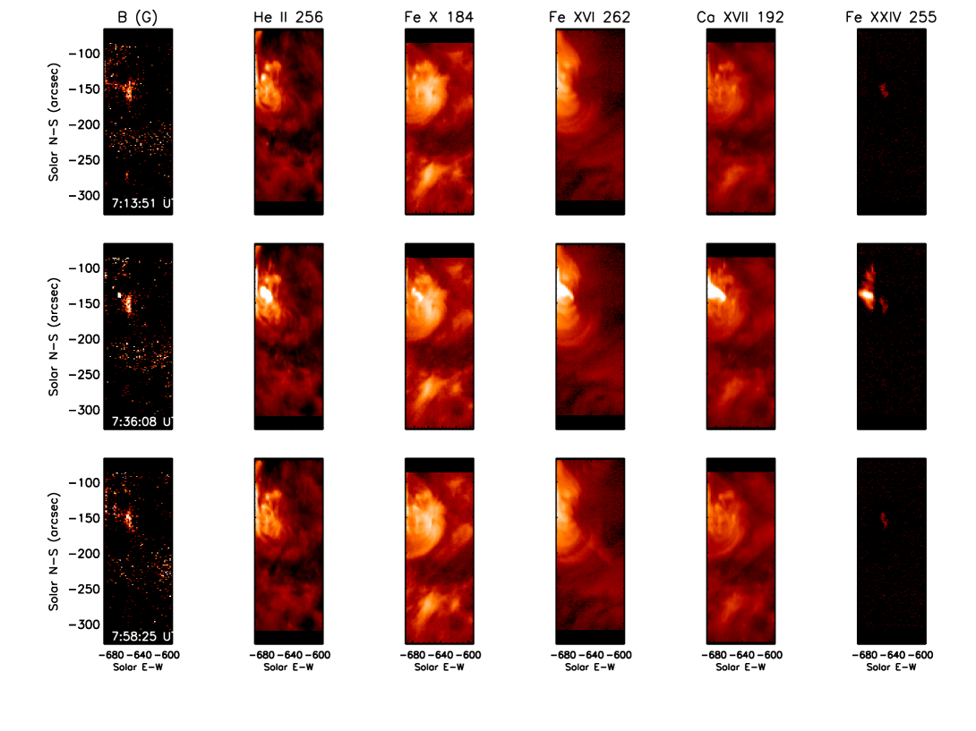
Figure 1: Intensity and magnetic field strength maps for three consecutive EIS rasters of AR10969, taken before, during and after the C2 flare. The flare can be seen in the 07:36 UT raster (middle row).

Figure 1 shows intensity maps as measured in five different spectral lines for each of three rasters across the active region, centered on the raster hosting the flare. The lines range in formation temperature from the chromosphere (He ii 256.32 Å), to the corona (Fe x 184.4 Å and Fe xvi 262.98 Å), and the flare (Ca xvii 192.85 Å and Fe xxiv 255.11 Å). The magnetic field strength map is also shown in the first column, showing that only in the region at the base of a coronal loop structure was the L20 magnetic field diagnostic technique able to detect magnetic field of strong enough to provide a significant measurement.

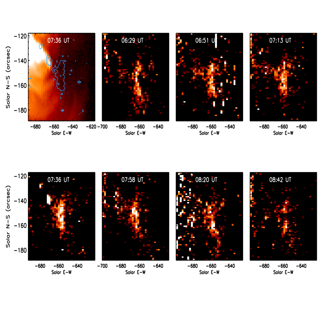
Figure 2: Maps of the magnetic field overlaying the sunspot in each of the first 7 observations. For reference, the intensity of the Fe xvi 262.98 Å line at 07:36 UT is shown in the top left panel, with the countours of the magnetic field measured at the same time overlaid on it. The MFE is present in the 07:36 UT (bottom-left) panel only and is located at the footpoint of the Fe xvi flare emission at 07:36 UT (top left panel).

A closer view of the evolution of the magnetic field in the active region is given in Figures 2 and 3; in the latter, the flare start time measured by GOES is indicated by the vertical red dashed line. In Figure 2, the morphology of the magnetic field is displayed, showing that the shape and distribution of the magnetic field significantly changed, with the size of the region with magnetic field stronger than $\approx$50 G slightly increasing before the flare (occurred in the 07:36 UT raster) and decreasing afterwards.

The average magnetic field strength, shown in the left panel of Figure 3, does not change significantly and is about 100 G, with the large uncertainty erasing the possibility of detecting any evolution. On the contrary, the total magnetic energy (right panel) shows some evolution, largely due to the change in size of the region filled with detectable magnetic field. This energy has been calculated (in erg) as

$$E_{tot}=10^{7}\frac{B^{2}}{2\mu_{0}}V$$ (3)

where $B$ is the magnetic field strength (in T), and $\mu_{0}$ is the permeability of free space. The volume $V$ of the region has been determined by multiplying the area (in $m^{2}$) of the image occupied by magnetic field larger than 50 G in each raster (which is the quantity that causes the energy variation in Figure 3, right) with an arbitrary average line-of-sight (LOS) depth of the magnetic field structure imaged by the Fe x emission of 1” (corresponding to 734 km, with a solar radius of 949” as seen from the Earth). It is important to stress that these energy values are only gross estimates, whose uncertainties stem from two main sources: 1) the uncertainty in the value of $B$ (around 70%, as suggested in L20); and 2) the complete lack of information about the LOS depth of the magnetic field region imaged by Fe x.

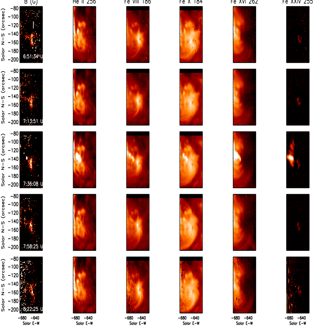
Figure 4: Close-ups of the magnetic field strength and intensity maps of the flaring active region. The flare occurred at 07:49 UT, and is observed in the 07:36 UT observation (middle row).

The evolution of the whole active region before, during and after the flare is shown in more detail in Figure 4. Except for the appearance of the Fe xxiv line in the 07:36 UT image, invisible in all other rasters, along with a brightening of variable intensity and shape in all other lines at the same time, the overall structure of the active region is largely untouched by the event. Also, the flare has no significant effect on the magnetic field with the only exception of a large magnetic field enhancement over a very small area in the 07:36 UT raster at around ${\left({-670",-140"}\right)}$. It is fair to say that the flare left the host active region relatively unscathed.

4.3 The flare Magnetic Field Enhancement

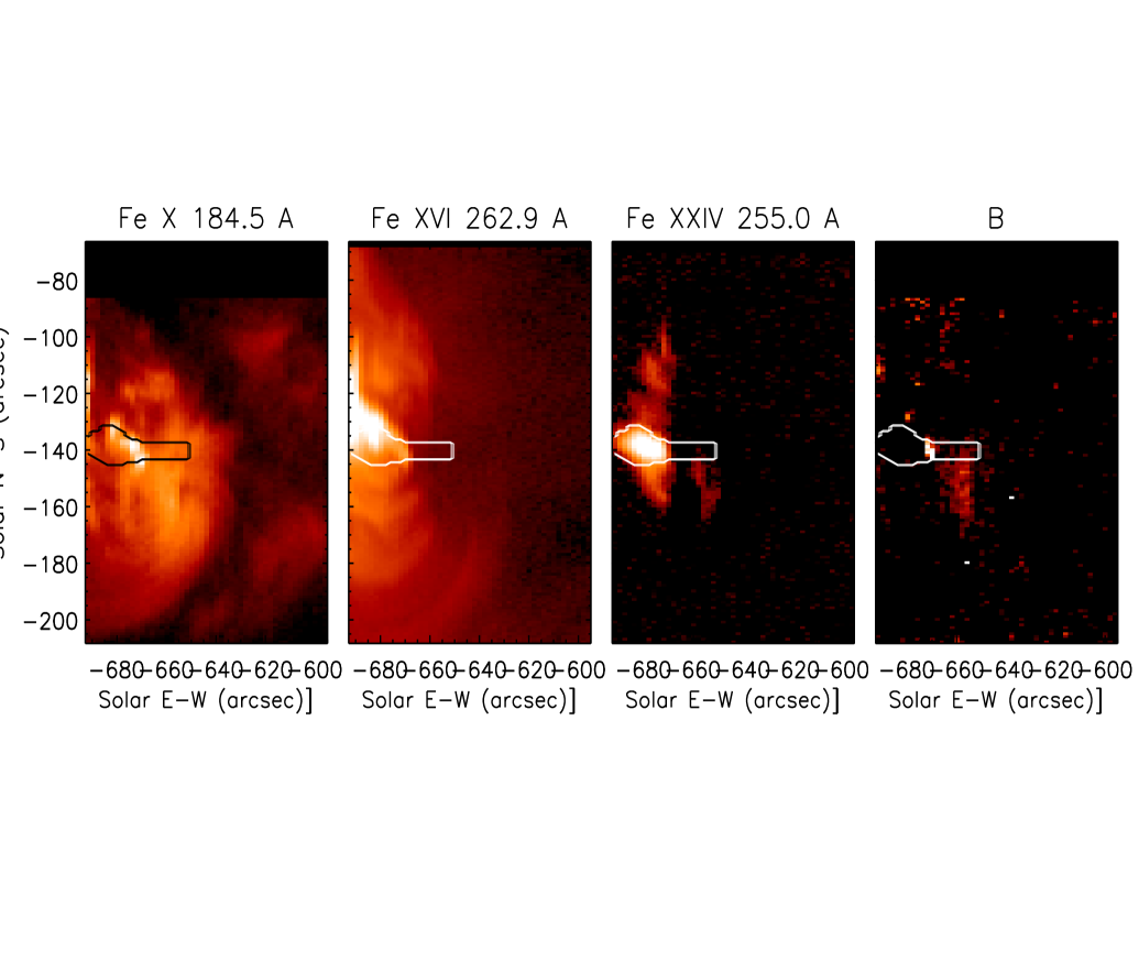
Figure 5: Magnetic field and intensity maps of the flaring active region from the 07:36 UT observation, with the pixels selected for diagnostics overlaid on them. The MFE is visible at two slit raster positions at (-670”,-140”).

The magnetic field enhancement (MFE) and its relationship to the flare emission are shown in the top left 07:36 UT panel in Figure 2, where it is overlaid (blue line) to the Fe xvi flare intensity taken at the same time. While the MFE seems to be unrelated to the active region magnetic field, it is located right at the footpoint of the Fe xvi flare intensity enhancement; Figure 5 confirms that this point lies at the footpoint of the flare emission of all lines, especially the Fe xxiv emission.

In order to measure the magnetic field strength and the flare properties, we have selected the pixels along the slit that include the flare emission, marked using the Fe xxiv 255.11 Å line, and the MFE, and extended the selection to pixels westward of the flare, at locations observed before the flare erupted, for comparison purposes. The selected pixels are shown in Figure 5. For each slit position, the emission has been averaged along the slit and used used to measure line intensities, plasma densities and the magnetic field strength.

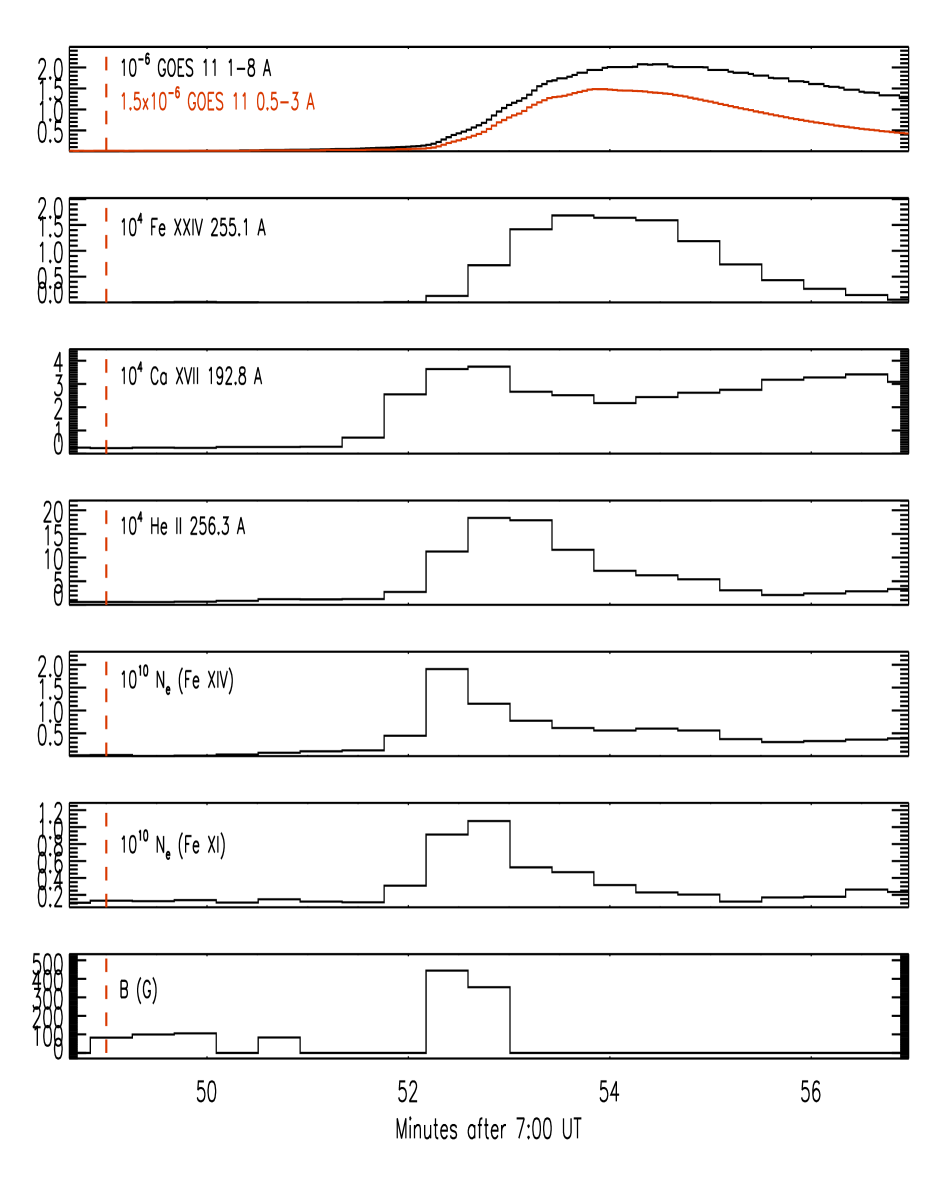
Figure 6: Light curves observed during the flare, from top to bottom: GOES-11 X-ray flux, the Fe xxiv 255.11 Å and Ca xvii 192.85 Å flare lines, the He ii 256.32 Å, the electron density from Fe xiv and Fe xi intensity ratios, and magnetic field strength B measured with the L20 diagnostic technique. The start of the GOES flare is marked by the red vertical dashed line.

Figure 6 shows the light curves of GOES-11, the Fe xxiv 255.11 Å and Ca xvii 192.85 Å flare lines, the He ii 256.32 Å line, and the electron density measured using the Fe xiv 264.24/274.20 and Fe xi 182.17/(188.22+188.30) line intensity ratios, along with the magnetic field measurement. The start of the flare as reported by GOES is indicated by the vertical red dashed line at 07:49 UT, on the left. What is extremely important to remember is that the rastering nature of the EIS observing sequence means that the EIS light curves are built using data taken as the slit was rastering, so that different times correspond to different locations within the active region, which might have been evolving differently from each other. Thus, a direct comparison between the GOES X-ray light curve and the EIS light curves is potentially misleading, as GOES was observing the Sun as a star and therefore includes the emission from the entire flare. Also, time variations in any of the EIS-related quantities might be equally due to either the flare time evolution or its spatial variability.

With this caveat in mind, Figure 6 allows us to draw several conclusions.

• First, EIS did not observe the location of the reconnection event triggering the flare, or at least reached it after reconnection occurred, as the flare effects were imaged by the instrument a few minutes later than the GOES start, indicating that the flare took place eastward of the location observed by EIS at 07:49 UT.

• Second, EIS started to observe significant flare emission and density enhancement around 2 minutes after the flare started, corresponding to 6 steps (12 arcsec) in the E-W direction: since the X-ray emission was still rapidly increasing when EIS reached the flare location, the energy release was still underway. A further confirmation of this comes from the Ca xvii light curve rising and peaking earlier than Fe xxiv, as expected in a rapidly heating plasma, unless multiple locations of energy injections were present.

• Third, the plasma density increases significantly from pre-flare values, with Fe xi and Fe xiv providing different estimates, indicating that plasma at different temperatures may belong to different structures below the EIS spatial resolution affected by the flare.

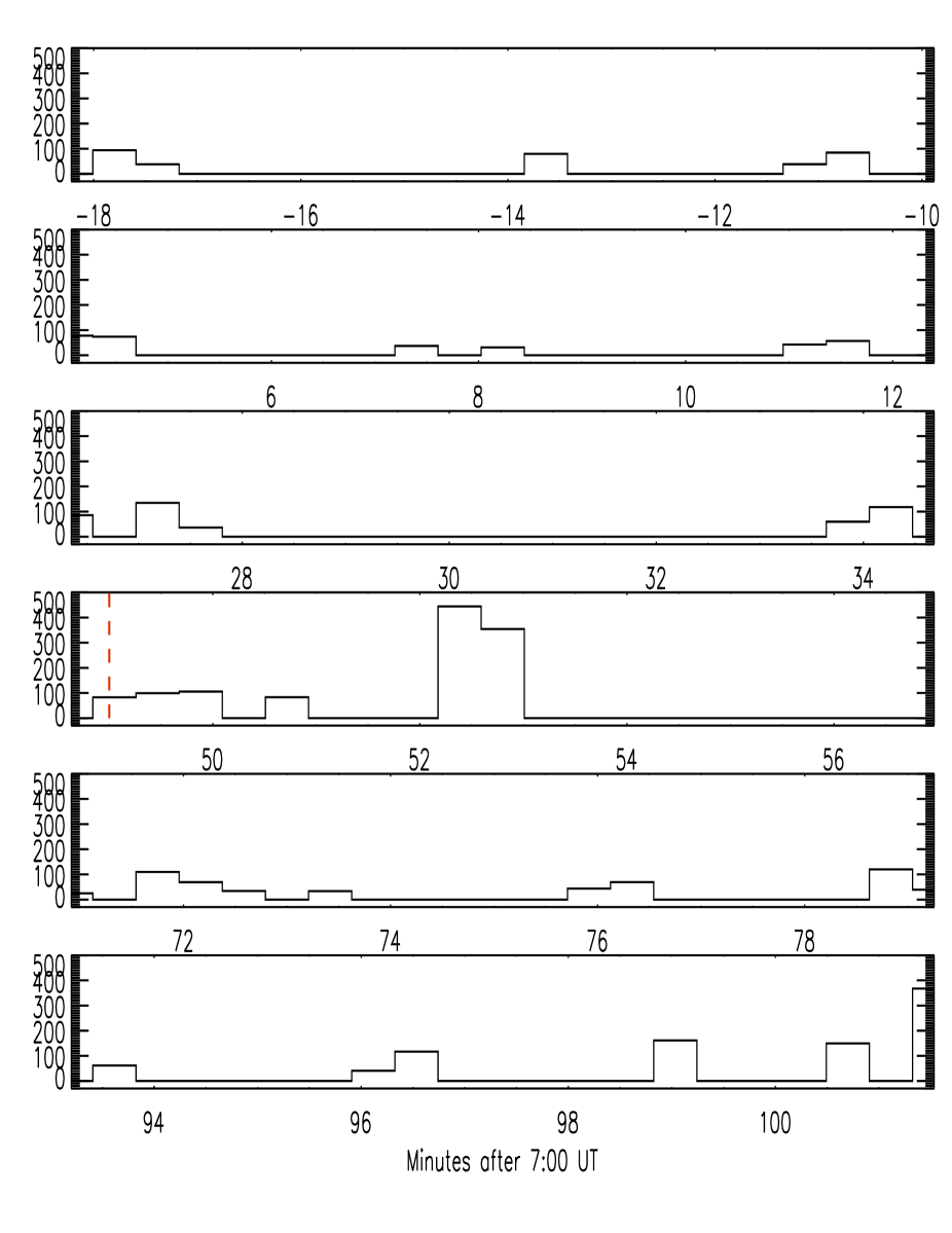
Figure 7: Magnetic field strength measured from the same pixels used to study the flare, along 6 consecutive EIS rasters, from 6:29 UT to 8:41 UT. Each time stamp on the X-axis of each row corresponds to a different pointing; however, the locations shown are the same for each consecutive raster.

However, the most stricking feature of Figure 6 is the presence of a strong MFE right at the locations where the line emission is rising and the electron density has spiked. This MFE is all the more striking as it occurs in a region where the magnetic field is below the detection threshold of the L20 technique when observed before the flare, and its spatial extent is very limited, being around 8 arcsec along the slit and just two raster positions (corresponding to 4 arcsec) along the E-W direction. This MFE is observed after the flare has already started (as shown by the GOES light curve, and even the Ca xvii intensity enhancement) and before the impulsive phase ends and energy is still being released. Also, this MFE is present only in the raster containing the flare: Figure 7 shows the magnetic field strength measured in 6 consecutive rasters at the same pixels selected for the flare, and clarly shows that no magnetic structure is present at the MFE location in the rasters before and after the flare.

Finally, the energy associated to this MFE is, according to Equation 3, around $8\times 10^{28}$ erg, again assuming arbitrarily that LOS length of the region where the magnetic field is enhanced is 1”. This energy is in good agreement with the typical total energy lost to radiation by a C2 flare, which lies in the $10^{28}-10^{30}$ erg range (Ryan et al. 2012). It is important to note that this energy has been obtained from measurements using the Weak Field regime, as discussed in Section 2, and thus represents a underestimate of the total energy. Still, despite the very large uncertainty in the actual value of the magnetic energy of the MFE, this measurement clearly shows that the MFE detected by the L20 technique is capable of providing enough energy to power the entire flare.

All these properties of the MFE point towards the following conclusions:

1. The MFE most likely takes place at the location of the magnetic reconnection event;

2. The MFE is strictly related to the flare event, having developed during the 22 minutes that EIS took to come back to the same location;

3. The MFE energy is sufficient to power the entire flare;

4. The enhanced magnetic field is dissipated during the flare to levels below the L20 technique threshold.

5 Discussion

The results of the present analysis indicate that a short impulsive C2 flare, with no visible effects on the structure of the host active region, is strictly associated to a relatively strong MFE (350-500 G) that formed right before the flare event, and was entirely dissipated during the flare event. This MFE is confined to a relatively small region (16$\times$2 arcsec²) where no specific plasma structure was visible before or after the flare, and leaves no trace after the flare ends. The magnetic energy associated to the MFE is compatible with typical total radiative losses from a C2 flare, and thus it is capable to power the flare itself.

These results open a lot more questions than they answer, and pose a formidable challenge to flare prediction efforts. Hopefully new observations from the EIS spectrometer will be devoted to flare hunts and will lead to a database of flares of all sizes that allow to improve on the present results and extend them to all flare classes.

The first conclusion that we can draw about flare predictability is that the quick formation of an MFE in an active region might be a precursor sign of a flare. While this provides a potential powerful tool for flare prediction, the short time that the MFE took to form (less than 22 minutes, corresponding to the return time of the EIS raster) poses a formidable challenge to flare prediction efforts, as it indicates that only a few minutes are available between the detection of the flare precursor formation and the actual flare.

Still, a C2 flare is a minor flare, and the properties of larger flares, with significant impact on Space Weather (M1.0 and higher) can be different, such as taking more time to form an MFE with enough energy to generate a more powerful flare. Furthermore, impulsive and long-duration flares might have different MFE formation processes and timescales.

The fact that we could only find one suitable flare dataset in the entire EIS range means that our results are just one point in the flare parameter space. They open the door to a host of future studies, which hopefully will answer the many questions which the present results can only ask:

1. Are MFEs a typical flare feature?

   1. What processes are responsible for MFE formation, and where within the active region do they form?

   2. How much time does an MFE need to form, and is this formation time correlated to the flare strength?

   3. Can MFE formation itself be predicted?

   4. Do all impulsive and long-duration flare produce MFEs, and are the formation processes and locations the same?

2. Can MFEs be used as flare precursors for Space Weather forecasting?

   1. If MFEs are indeed flare precursors, which flare prediction success rate would they allow us to reach?

   2. What advance warning time can MFEs give us for a flare event?

Also, many issues about the L20 technique itself need to be addressed in order to make the estimate of the magnetic field strength and energy more accurate. These issues mainly concern the calibration of the EIS instrument, which is the main source of uncertainty in the determination of an absolute value of the MFE magnetic field strength and energy.

References

1. Acuna, M.H., Ogilvie, K.W., Baker, D.N., et al. 1995, Sp. Sci. Rev. 71, 5

2. Benz, A. 2017, Liv. Rev. Sol. Phys., 14, 2

3. Chen, J., Liu, R., Liu, K., et al. 2020, ApJ, 890, 158

4. Culhane, J.L., Harra, L.K., James, A.M., et al. 2007, Sol. Phys., 243, 19

5. Fletcher, L., Dennis, B.R., Hudson, H.S. et al. 2011, Sp. Sci. Rev, 159, 19

6. Harra, L.K., Matthews, S.A., & Culhane, J.L. 2001, ApJ, 549, L245

7. Harra, L.K., Williams, D.R., Wallace, A.J., et al. 2009, ApJ, 691, L99

8. Jiao, Z., Sun, H., Wang, X., et al. 2020, Sp. Weather, 18, e2020SW002440

9. Kosugi, T., Matsuzaki, K., Sakao, T., et al. 2007, Sol. Phys., 243, 3

10. Landi, E., Hutton, R., Brage, T., & Li, W. 2020, ApJ, 904, 87

11. Li, W., Grumer, J., Yang, Y., et al. 2015, ApJ, 807, 69

12. Li, W., Yang, Y., Tu, B., et al. 2016, ApJ, 826, 219

13. Li, W., Li, M.,Wang, K., Brage, T., Hutton, R., Landi, E. 2021, ApJ submitted

14. Pulkkinen, T. 2007, Liv. Rev. Sol. Phys, 4, 1

15. Ryan, D.F., Milligan, R.O., Gallagher, P.T., et al. 2012, ApJS, 202, 11

16. Si, R., Brage, T., Li, W., et al. 2020a, ApJL, 898, L34

17. Si, R., Li, W., Brage, T., & Hutton, R. 2020b, J. Phys. B, 53, 095002

18. Stone, E.C., Frandsen, A.M., Mewaldt, R.A., et al. 1998, Sp. Sci. Rev., 86, 1

19. Wang, X., Cheng, Y., Toth, G., et al. 2020, ApJ, 895, 3

20. Webb, D.F., & Howard, T.A. 2012, Liv. Rev. Sol. Phys., 9, 3

21. Woods, T.N., Hock, R., Eparvier, F., et al. 2011, ApJ, 739, 59

Figure 3: Average magnetic field overlying the sunspot, as shown in Figure 2, and magnetic energy associated to it.