TESS Hunt for Young and Maturing Exoplanets (THYME) IV: Three small planets orbiting a 120 Myr-old star in the Pisces–Eridanus stream

Abstract

Young exoplanets can offer insight into the evolution of planetary atmospheres, compositions, and architectures. We present the discovery of the young planetary system TOI 451 (TIC 257605131, Gaia DR2 4844691297067063424). TOI 451 is a member of the 120-Myr-old Pisces–Eridanus stream (Psc–Eri). We confirm membership in the stream with its kinematics, its lithium abundance, and the rotation and UV excesses of both TOI 451 and its wide binary companion, TOI 451 B (itself likely an M dwarf binary). We identified three candidate planets transiting in the TESS data and followed up the signals with photometry from Spitzer and ground-based telescopes. The system comprises three validated planets at periods of $1.9$, $9.2$ and $16$ days, with radii of $1.9$, $3.1$, and $4.1$ $R_{\earth}$, respectively. The host star is near-solar mass with $V=11.0$ and $H=9.3$ and displays an infrared excess indicative of a debris disk. The planets offer excellent prospects for transmission spectroscopy with HST and JWST, providing the opportunity to study planetary atmospheres that may still be in the process of evolving.

1 Introduction

Exoplanets are expected to undergo significant evolution in the first few hundred million years of their lives, including thermal and compositional changes to their atmospheres and dynamical evolution. Stellar high energy irradiation, which diminishes with age, impacts atmospheric mass loss rates (e.g. Jackson et al., 2012; Kubyshkina et al., 2018) and atmospheric chemistry (e.g. Segura et al., 2005; Gao & Zhang, 2019). These processes can have a dramatic effect on the observed properties of planets with sizes in between those of Earth and Neptune.

Atmospheric mass loss is thought to be responsible for the observed “radius valley”, a deficit of planets $1.5-2$$R_{\earth}$ and the accompanying bimodality of the radius distribution (Owen & Wu, 2013; Fulton et al., 2017). This valley was predicted by photoevaporation models, where mass loss is driven by high energy radiation from the host star (Lopez & Fortney, 2013; Owen & Wu, 2013; Jin et al., 2014). Comparison of models to the data by Owen & Wu (2017) and Jin & Mordasini (2018) support this interpretation. However, core-powered mass-loss, in which the atmospheric loss is driven by the luminosity of the hot planetary interior, is also successful at explaining the radius valley (Ginzburg et al., 2018; Gupta & Schlichting, 2019). The timescale for core-powered mass loss is $\sim$1 Gyr (Gupta & Schlichting, 2020), in contrast to $\sim$100 Myr for photoevaporation (Owen & Wu, 2017). Alternatively, Zeng et al. (2019) and Mousis et al. (2020) propose that the 2–4 $R_{\earth}$ planets are water worlds, with compositions reflecting the planets’ accretion and migration history. Lee & Connors (2020) consider formation in gas-poor environments to argue that the radius valley is primordial.

Planets larger than $\sim 1.6$$R_{\earth}$ are expected to have gas envelopes constituting $\gtrsim 1$% of the core mass (Rogers, 2015; Wolfgang & Lopez, 2015); and their atmospheric compositions and chemistry can be probed with transmission spectroscopy (e.g. Seager & Sasselov, 2000; Miller-Ricci et al., 2009). The observed spectra of these planets range from flat and featureless (Knutson et al., 2014; Kreidberg et al., 2014) to exhibiting the spectral fingerprints of water (Fraine et al., 2014; Benneke et al., 2019; Tsiaras et al., 2019). Featureless spectra may result from clouds or hazes present at low atmospheric pressures (e.g. Morley et al., 2015). Gao & Zhang (2019) quantified how hazes can also result in large optical depths at low pressures (high altitudes), which results in larger planetary radii than would otherwise be measured. Gao & Zhang (2019) find that this effect would be most important in young, warm, and low-mass exoplanets, for which outflows result in high altitude hazes.

The theories make different predictions about atmospheric properties and the timescale for changes. Therefore, the compositions and atmospheric properties of individual young exoplanets, and the distribution of young planet radii can constrain these theories. Transmission spectroscopy of young planets may also allow atmosphere composition measurements where older planets yield flat spectra, if relevant atmospheric dynamics or chemistry change with time.

The Transiting Exoplanet Survey Satellite (TESS; Ricker et al., 2015) mission provides the means to search for young exoplanets that orbit stars bright enough for atmospheric characterization and mass measurements. The TESS Hunt for Young and Maturing Exoplanets (THYME) Survey seeks to identify planets transiting stars in nearby, young, coeval populations. We have validated three systems to date: DS Tuc A b (Newton et al., 2019), HIP 67522 b (Rizzuto et al., 2020), and HD 63433 b and c (Mann et al., 2020). Our work complements the efforts of other groups to discover young exoplanets, such as the Cluster Difference Imaging Photometric Survey (CDIPS; Bouma et al., 2019) and the PSF-based Approach to TESS High quality data Of Stellar clusters project (PATHOS; Nardiello et al., 2019).

The unprecedented astrometric precision from Gaia (Gaia Collaboration et al., 2016, 2018) and TESS’s nearly all-sky coverage combined to create an opportunity for the study of young exoplanets that was not previously available. Meingast et al. (2019) conducted a search for dynamically cold associations in phase space using velocities and positions from Gaia. They identified a hitherto unknown stream extending 120$\degree$ across the sky at a distance of only 130 pc, which was called the Pisces–Eridanus stream (Psc–Eri) by Curtis et al. (2019). Meingast et al. (2019) found that the 256 sources defined a main sequence, and based on the presence of a triple system composed of three giant stars, they suggested an age of $\sim$1 Gyr. Curtis et al. (2019) extracted TESS light curves for a subset of members and measured their rotation periods. Finding that the stellar temperature–period distribution closely matches that of the Pleiades at 120 Myr, they determined that the stream is similarly young. Color–magnitude diagrams from Curtis et al. (2019), Röser & Schilbach (2020), and Ratzenböck et al. (2020), and lithium abundances from Arancibia-Silva et al. (2020) and Hawkins et al. (2020a), support the young age.

The Psc–Eri stream offers a new set of young, nearby stars around which to search for planets. The stream complements the similarly-aged Pleiades, in which no exoplanets have been found to date. Thanks to the nearly all-sky coverage of TESS, photometry that could support a search for planets orbiting Psc–Eri members was already available when the stream was identified. We cross-matched the TESS Objects of Interest (Guerrero, submitted) alerts to the list of Psc–Eri members from Curtis et al. (2019), and found TOI 451 to be a candidate member of the stream.

We present validation of three planets around TOI 451 with periods of $1.9$ d (TOI 451 b), $9.2$ d (TOI 451 c) and $16$ d (TOI 451 d). In Section 2, we present our photometric and spectroscopic observations. In Section 3, we discuss our measurements of the basic parameters and rotational properties of the star. We find that TOI 451 is a young solar-mass star, and has a comoving companion, Gaia DR2 4844691297067064576, that we call TOI 451 B. We address membership of TOI 451 and TOI 451 B to the Psc–Eri stream in Section 4 through kinematics, abundances, stellar rotation, and activity. We model the planetary transits seen by TESS, Spitzer, PEST, and LCO in Section 5, and conclude in Section 6. Appendix A describes our analysis of GALEX  and demonstrates UV excess as a way to identify new low-mass members of Psc–Eri.

2 Observations

2.1 Time-series photometry

After the initial discovery of the signal in the TESS data (Figure 1), we obtained follow-up transit photometry from the Las Cumbres Observatory (LCO; Brown et al., 2013), the Perth Exoplanet Survey Telescope (PEST), and the Spitzer Space Telescope (Figure 2). Table 1 lists the photometric data modeled in Section 5.1; this subset of the available data provided the best opportunity for constraining the transit model. These and additional ground-based lightcurves ruled out eclipsing binaries on nearby stars, found the transit to be achromatic, and confirmed TOI 451 as the source of the three candidate event.

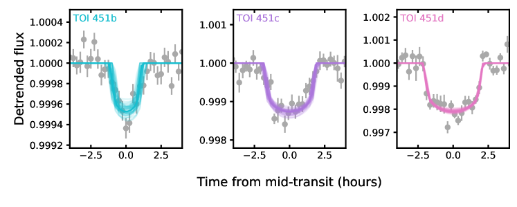
Figure 1: TESS data and models. Top panel: TESS lightcurve (gray points) with the Gaussian process (GP) model to stellar variability overlain (blue). The mean (opaque line) and 68% confidence limits (semi-transparent regions) of the stellar variability model are shown. Marked at the bottom are transit times of each of the three planets, with TOI 451 b in teal, c in purple, and d in pink. Bottom panel: the phase-folded data centered on the transit of each planet, after the best-fit stellar variability model has been removed and the transits of other planets have been masked. The best-fit transit models (opaque lines) are overplotted along with 50 draws from the posterior distribution (semi-transparent lines). Both the data and the models have been binned into 15 minute bins. Note that small changes in the binning will cause the perceived shape of the plotted transit data to change.

Figure 2: Follow-up photometry (gray points) and model (solid lines). The model without the transit is also shown (dashed lines). The model shown is the best-fit transit model for the case where eccentricities are fixed to 0. 50 draws from the posterior are also overplotted. Top two rows: Spitzer data and models. No stellar variability is modeled for Spitzer transits. Bottom row: Ground-based observatory data and models, with PEST on the left and LCO in the center. Stellar variability is modeled for these data.

Table 1: Photometry used in this paper

Telescope	Filter	Date	Planet	AOR
TESS	TESS	2018-10-19	…	…
		–2018-12-11	…	…
PEST	$Rc$	2019-11-05	d	…
LCO-CTIO	$z_{s}$	2019-12-08	d	…
Spitzer	Ch2	2019-06-11	d	69684480
		2019-12-24	d+b	70049024
		2019-12-26	c	70048512
		2020-01-09	d	70048768
		2020-01-13	c	70048256

Note. — In the text, Spitzer transits are referred to be the AOR ID (last column). Spitzer AOR 69684480 obtained through GO program 14084 (PI: Crossfield); remaining AORs through GO program 14011 (PI: Newton).

2.1.1 TESS

TESS observed TIC 257605131 in Sectors 4 and 5, from 2018 October 19 to 2018 December 11. TIC 257605131 was identified as a promising target to support TESS’s prime mission by Stassun et al. (2018); it was included in the Candidate Target List (CTL) and thus observed at 2 minute cadence. The data were processed by the Science Processing and Operations Center (SPOC) pipeline (Jenkins et al., 2016), which calibrated and extracted the data, corrected the lightcurve, and finally filtered the light curve and searched for planets. The identified signal passed visual vetting, and the community was notified via alerts along with other TESS candidate planets (Guerrero, submitted).

The original TESS alert identified one candidate, TOI 451.01, at a period of $8$ days. Our initial exploration with EXOFAST (Eastman et al., 2013) suggested that the $8$ day signal is a combination of two real but distinct transit signals, and yielded two candidates, at $9.2$ and $16$ days. Throughout follow-up, these signals were referred to as TOI 451.02 and 451.01, respectively. Another candidate was added as a community TOI to ExoFOP, identified as TIC 257605131.02, at a period of $1.9$ days. The candidate was also identified in the results of two independent pipelines run by our team. We now identify the $1.9$-day planet as TOI 451 b, the $9.2$-day as TOI 451 c and the $16$-day as TOI 451 d.

The presence of all three planets is supported by the TESS data. Our custom pipeline (Rizzuto et al., 2017, 2020) identified all three planets, with signal-to-noise ratio (S/N) $=14.8$, $13.9$, and $10.4$ (for planet detection, we typically adopt a threshold of S/N $=7$). TOI 451 d was also found at the correct period in the SPOC multi-sector transit search. The transit detection statistic was $12.2$. It had a clean data validation report (Twicken et al., 2018; Li et al., 2019) and passed the odd-even depth test, the difference image centroiding and ghost diagnostic test, which can reveal background eclipsing binaries. The only diagnostic test it failed was the statistical bootstrap test, which was due to the transits of the other planets in the light curve that were not identified. TOI 451 c narrowly missed detection with a transit detection statistic of $7.05$.

We used the presearch data conditioning simple aperture photometry (PDCSAP_FLUX) light curve produced by the SPOC pipeline (Stumpe et al., 2012; Smith et al., 2012; Stumpe et al., 2014). Prior to using these data for our transit fit, we removed flares by iteratively fitting the Gaussian Process model described in §5 using least-squares regression. We first masked the transits and iterated the GP fitting, rejecting outliers at each of three iterations. We then detrended the lightcurve using the fitted GP model, and removed outliers from the detrended lightcurve. We removed $3.5\sigma$ outliers and iterated until no additional points were removed, removing a total of 47 data points.

2.1.2 Spitzer

We obtained transit observations of TOI 451 c and d at $4.5\micron$ (channel 2) with Spitzer’s Infrared Array Camera (IRAC; Fazio et al., 2004), one on 2019 June 11 (UT) and four between 2019 December 24 and 2020 January 13 (UT). Dates and AOR designations, which we use to identify the Spitzer transits, are in Table 1.

We used $2$ second frames and the $32\times 32$ pixel subarray. We placed the target on the detector “sweet spot” and used the “peak-up” pointing mode to ensure precise pointing (Ingalls et al., 2012, 2016). For AORs 70049024, 70048512, 70048768, and 70048256, we scheduled a 20 min dither, then an 8.5 hr stare covering the transit, followed by a 10 minute dither. For AOR 69684480, we scheduled a 30 min dither, 8.7 hr stare, and 15 min dither. Though we had not considered TOI 451 b at the time of scheduling Spitzer observations, a transit of TOI 451 b happened to coincide with one of our transits of TOI 451 d.

We extracted time-series photometry and pixel data from the Spitzer AORs following the procedure described in Livingston et al. (2019). Apertures of 2.2-2.4 pixels were used, selected based on the algorithm to minimize both red and white noise also described in that work. We used pixel-level decorrelation (PLD; Deming et al., 2015) to model the systematics in the Spitzer light curves, which are caused by intra-pixel sensitivity variations coupled with pointing jitter. We used the exoplanet package (Foreman-Mackey et al., 2019) to jointly model the transit and systematics in each Spitzer light curve, assuming Gaussian flux errors. We assume a circular orbit. For the prior on the limb-darkening parameters, we used the values tabulated by Claret & Bloemen (2011) in accordance to the stellar parameters. We placed priors on the stellar density, planetary orbital period, planet-to-star radius ratio ($R_{p}/R_{s}$), and expected time of transit based on an initial fit to only the TESS data. For all planetary parameters, the priors were wider than the posterior distributions, so the data provides the primary constraint. We obtained initial maximum a posteriori (MAP) parameter estimates via the gradient-based BFGS algorithm (Nocedal & Wright, 2006) implemented in scipy.optimize. We then explored parameter space around the MAP solution via the NUTS Hamiltonian Monte Carlo sampler (Hoffman & Gelman, 2014) implemented in PyMC3. We confirmed the posteriors were unimodal and updated the MAP estimate if a higher probability solution was found.

The two transits of c (AORs 70048512 and 70048256) and solely of d (AORs 69684480 and 70048768) were fit simultaneously. For AOR 70049024, the model consisted of overlapping transits of TOI 451 b and d, and we fixed the limb-darkening parameters. Trends were included where visual inspection of the model components showed that PLD alone was not sufficient to explain the data, i.e. due to stellar variability; for AORs 69684480 and 70048512, quadratic terms were used. We then computed PLD-corrected light curves by subtracting the systematics model corresponding to the MAP sample from the data. We use these corrected Spitzer datasets for the subsequent transit analyses in §5.

The inclusion of TOI 451 b overlapping the transit of d in AOR 70049024 was strongly favored by the data per the Bayesian Information Criterion (BIC). The two-planet model had $\Delta$BIC$=27$ compared to the model with only TOI 451 d. Prior to realizing the transit of TOI 451 b was present, we had also considered a model with TOI 451 d and a Gaussian Process. The two-planet model had $\Delta$BIC$=7.7$ compared to this model.

2.1.3 Investigation into Spitzer systematics

With the joint PLD fit of the two Spitzer transits of TOI 451 c, we consistently modeled both ($R_{P}/R_{*}=0.034\pm 0.001$). However, there was a $5\sigma$ discrepancy between the depths of the two transits when we used PLD as described above, but reduced each independently ($R_{P}/R_{*}=0.037\pm 0.001$ for AOR 70048512; $R_{P}/R_{*}=0.026\pm 0.002$ for AOR 70048256). The difference in the two transit depths, obtained 18.5 days apart, is difficult to explain astrophysically, especially given the expectation for decreased stellar variability at $4.5\micron$. We hypothesize that this results from the low signal-to-noise ratio of the transits, but the discrepancy in the independent fits raised concerns about systematic effects in the Spitzer data.

To investigate systematics in these data further, we additionally used the BiLinearly-Interpolated Subpixel Sensitivity (BLISS) mapping technique to produce an independent reduction of the Spitzer data for TOI 451 c. BLISS uses a non-parametric approach to correct for Spitzer’s intrapixel sensitivity variations.

We processed the Spitzer provided Basic Calibrated Data (BCD) frames using the Photometry for Orbits, Eccentricities, and Transits (POET; Stevenson et al. 2012; Campo et al. 2011) pipeline to create systematics-corrected light curves. This included masking and flagging bad pixels, and calculating the Barycentric Julian Dates for each frame. The center position of the star was fitted using a two-dimensional, elliptical Gaussian in a 15 pixel square window centered on the target’s peak pixel. Simple aperture photometry was performed using a radius of 2.5 pixels, an inner sky annulus of 7 pixels, and an outer sky annulus of 15 pixels.

To correct for the position-dependent (intra-pixel) and time-dependent (ramp) Spitzer systematics, we used the BLISS Mapping Technique, provided through POET. We used the most recent 4.5$\mu$m intra-pixel sensitivity map from May & Stevenson (2020). The transit was modeled using the Mandel & Agol (2002) transit model and three different ramp parameterizations: linear, quadratic, and rising exponential, as well as a no-ramp model. The time-dependent component of the model consisted of the mid-transit time, $R_{p}/R_{s}$, orbital inclination ($\cos{i}$), semi-major axis ratio, system flux, ramp phase, ramp amplitude, and ramp constant offset. These parameters were explored with an Markov Chain Monte Carlo (MCMC) process, using 4 walkers with 500,000 steps and a burn-in region of 1,000 steps. The period was fixed to 9.19 days based on the TESS data, and starting locations for the MCMC fit were based on test runs.

To determine the best ramp models, we used two metrics: 1) overall minimal red noise levels in the fit residual, assessed by considering the root-mean-squared (rms) binned residuals as a function of different bin sizes with the theoretical uncorrelated white noise; and 2) Bayesian Information Criterion (BIC; e.g., Cubillos et al., 2014). Low rms and low BIC are favored.

For AOR 70048512, significant red noise remained for the no-ramp model and was present to a lesser degree with the other ramp models. However, the no-ramp model yielded the lowest BIC value, while quadratic and rising exponential ramps yielded the largest but had lower red noise. There was a discrepancy in the transit depth for the different ramp parameterizations: no-ramp and the linear ramp returned $R_{P}/R_{*}$ of $0.031\pm 0.001$ and $0.032\pm 0.001$, respectively, while the quadratic and exponential ramps each returned $0.036\pm 0.001$ (in comparison to the PLD independent fit of this transit with $R_{P}/R_{*}=0.037\pm 0.001$).

For AOR 70048256, we obtained consistent transit depths of around $0.032$ with all four BLISS ramp options with typical error $\pm 0.002$ (in comparison to the PLD independent fit of this transit with $R_{P}/R_{*}=0.027\pm 0.003$). No significant red noise was present in any of the ramp models. The no-ramp model yielded the lowest BIC value, while the quadratic and rising exponential ramp models yielded the largest.

This exploration demonstrated that the transit depths were sensitive to ramp choice and the metric used to select the best fit (e.g., lowest BIC, lowest red noise, best agreement with TESS). We conclude that additional systematic errors in the Spitzer transit depths are likely present and are not accounted for in the analysis presented in §5.1.

2.1.4 LCO

We observed a transit of TOI 451d in Pan-STARRS $z$-short band with the LCO (Brown et al., 2013) 1 m network node at Cerro Tololo Inter-American Observatory on the night of 2019 December 08. We used the TESS Transit Finder, which is a customised version of the Tapir software package (Jensen, 2013), to schedule our transit observation. The images were calibrated by the standard LCOGT BANZAI pipeline (McCully et al., 2018) and the photometric data were extracted using the AstroImageJ (AIJ) software package (Collins et al., 2017). We used a circular aperture with radius 12 pixels to extract differential photometry. The images have stellar point-spread-functions (PSFs) with FWHM $\sim 2\farcs 5$.

2.1.5 PEST

We observed a transit egress of TOI 451d in the $Rc$-band with PEST on 2019 Nov 05 (UT). PEST is a 12 inch Meade LX200 SCT Schmidt-Cassegrain telescope equipped with a SBIG ST-8XME camera located in a suburb of Perth, Australia. We used a custom pipeline based on C-Munipack to calibrate the images and extract the differential time-series photometry. The transiting event was detected using a $7\farcs 4$ aperture centered on the target star. The images have typical PSFs with a FWHM of $\sim 4\arcsec$.

2.1.6 WASP-South

WASP-South is an array of 8 cameras located in Sutherland, South Africa. It is the Southern station of the WASP transit-search project (Pollacco et al., 2006). WASP-South observed available fields with a typical 10-min cadence on each clear night. Until 2012, it used 200-mm, f/1.8 lenses with a broad $V$+$R$ filter, and then switched to 85-mm, f/1.2 lenses with an SDSS-$r$ filter. TOI 451 was observed for 150 nights in each of 2006, 2007 and 2011 (12 600 data points) and for 170 nights in each of 2012, 2013 and 2014 (51 000 data points).

2.2 Spectroscopy

We obtained spectra with the Southern Astrophysical Research (SOAR) telescope/Goodman, South African Extremely Large Telescope (SALT)/High Resolution Spectrograph (HRS), Las Cumbres Observatory (LCO)/Network of Robotic Echelle Spectrographs (NRES), and Small and Moderate Aperture Research Telescope System (SMARTS)/CHIRON. The Goodman spectrum was used to fit the spectral energy distribution (§3.1.1); and the SALT, LCO, and CHIRON spectra to measure radial velocities (RVs; §3.3). The S/N of the spectra used for RVs are given in Table 3.

2.2.1 SOAR/Goodman

We obtained a spectrum of TOI 451 with the Goodman High-Throughput Spectrograph (Clemens et al., 2004) on the Southern Astrophysical Research (SOAR) 4.1 m telescope located at Cerro Pachón, Chile. On 2019 Dec 3 (UT), we took five exposures of TOI 451with the red camera, the 1200 l/mm grating in the M5 setup, and the 0.46″ slit rotated to the parallactic angle. This setup yielded a resolution of $R\simeq 5900$ spanning 6250–7500Å. To account for drifts in the wavelength solution, we obtained Ne arc lamp exposures throughout the night. We took standard calibration data (dome/quartz flats and biases) during the preceeding afternoon.

We performed bias subtraction, flat fielding, optimal extraction of the target spectrum, and found the wavelength solution using a 4th-order polynomial derived from the Ne lamp data. We then stacked the five extracted spectra using the robust weighted mean (for outlier removal). The stacked spectrum had S/N$>100$ over the full observed wavelength range.

2.2.2 SALT/HRS

We obtained six epochs with HRS (Crause et al., 2014) on SALT (Buckley et al., 2006) between 2019 July and 2019 October. Each epoch consisted of three back-to-back exposures. We used the high-resolution mode, ultimately obtaining an effective resolution of 46,000. Flat-fielding and wavelength calibration were performed using the MIDAS pipeline (Kniazev et al., 2016, 2017).

2.3 LCO/NRES

We observed TOI 451 twice using NRES (Siverd et al., 2018) on the LCO system. NRES is a set of cross-dispersed echelle spectrographs connected to 1 m telescopes within the Las Cumbres network, providing a resolving power of $R=53,000$ over the range $3800-8600$ Å. We took both observations at the Cerro Tololo node, the first on 2019 March 27 and the second on 2019 Jul 31 (UT). The March observation consisted of two back-to-back exposures. The standard NRES pipeline reduced extracted, and wavelength calibrated both observations.

2.4 SMARTS/CHIRON

We obtained a single spectrum with the CHIRON spectrograph (Tokovinin et al., 2013) on SMARTS, from which we measured the radial velocity and rotational broadneing of the star. CHIRON is a $R=80,000$ high resolution fiber bundle fed spectrograph on the 1.5 m SMARTS telescope, located at located at Cerro Tololo Inter-American Observatory (CTIO), Chile. Data were reduced according to Tokovinin et al. (2013).

2.5 Speckle Imaging

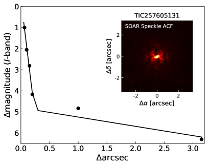
Figure 3: Detection limits (5$\sigma$) for companions to TOI 451 from SOAR speckle imaging.

To rule out unresolved companions that might impact our interpretation of the transit, we obtained speckle imaging using the High-Resolution Camera (HRCam) on the SOAR telescope. We searched for sources near TOI 451 in SOAR speckle imaging obtained on 17 March 2019 UT in $I$-band, a similar visible bandpass as TESS. Further details of observations from the SOAR TESS survey are available in Ziegler et al. (2020). We detected no nearby stars within $3\arcsec$ of TOI 451 within the $5\sigma$ detection sensitivity of the observation (Figure  3).

2.6 Gaia astrometry

2.6.1 A wide binary companion

The Gaia DR2 catalog (Gaia Collaboration et al., 2018) includes one co-moving, co-distant neighbor at $\rho=37.8$″  ($\rho=4700$ AU), TIC 257605132 (Gaia DR2 4844691297067064576). Aside from entries in all-sky catalogs, this neighbor star is unremarkable and does not appear to have been previously studied in the astronomical literature. Though this companion is only about two TESS pixels away from TOI 451, our high spatial resolution Spitzer data definitively rule it out as the source of the transits.

The parallax difference between TOI 451 and its neighbor is consistent with zero at 1.2$\sigma$, and the relative velocity in the plane of the sky ($\Delta\mu=0.21\pm 0.09$ mas/yr; $\Delta v_{\mathrm{tan}}=0.12\pm 0.05$ km/s) is lower than the circular orbital velocity for a total pair mass of $M\sim 1.2M_{\odot}$ and a projected distance of $4700$ AU. The relative astrometry and kinematics are thus consistent with a bound binary system and much lower than the typical velocity dispersion of $\sim$1 km/s seen in young associations. The separation is also within the semi-major axis range range commonly seen for bound binary pairs among young low-density associations (Kraus & Hillenbrand, 2008) and the field solar-type binary distribution (Raghavan et al., 2010). We therefore concluded that TIC 257605132 is a bound binary companion to TOI 451, and hereafter refer to it as TOI 451 B.

TOI 451 B has Gaia DR2 parameters of $B_{P}-R_{P}=2.527$ mag and $T_{\mathrm{eff}}=3507$ K. The color corresponds to a spectral type of M3V according to Kiman et al. (2019). TOI 451 B itself is likely a binary, as its Renormalized Unit Weight Error (RUWE; Lindegren et al., 2018) is $RUWE=1.24$, higher than the distribution typically seen for single stars and indicative of binarity (Rizzuto et al. 2018; Kraus et al., in preparation). We compared TOI 451 B’s location in the $G-R_{P}$ vs. $M_{G}$ color–magnitude diagram to the similarly-aged Pleiades population from Lodieu et al. (2019); it lies 0.65 mag above the main-sequence locus. We assumed TOI 451 B is comprised of two near-equal mass stars, and adjusted the reported 2MASS $K$ magnitude ($K=10.76$ mag) by 0.65 mag to match the main sequence locus. We then applied the mass-$M_{K}$ relation from Mann et al. (2019), which resulted in a mass of $0.45$ $\text{M}_{\odot}$. This mass is in agreement with the expectations for a star of the observed Gaia DR2 color for TOI 451 B.

2.6.2 Limits on Additional Companions

Our null detection from speckle interferometry is consistent with the deeper limits set by the lack of Gaia excess noise. TOI 451 has $RUWE=0.91$, consistent with the distribution of values seen for single stars. Based on a calibration of the companion parameter space that would induce excess noise (Rizzuto et al. 2018; Belokurov et al. 2020; Kraus et al., in preparation), this corresponds to contrast limits of $\Delta G\sim 0$ mag at $\rho=30$ mas, $\Delta G\sim 4$ mag at $\rho=80$ mas, and $\Delta G\sim 5$ mag at $\rho\geq 200$ mas. Given an age of $\tau=120$ Myr at $D=124$ pc, the evolutionary models of Baraffe et al. (2015) would imply corresponding physical limits for equal-mass companions at $\rho\sim 4$ AU, $M\sim 0.45M_{\odot}$ at $\rho\sim 10$ AU, and $M\sim 0.30M_{\odot}$ at $\rho>25$ AU.

Other than TOI 451 B, Gaia DR2 does not report any other comoving, codistant neighbors within an angular separation of $\rho<600\arcmin$ ($\rho<75,000$ AU) from TOI 451. At separations beyond this limit, any neighbor would be more likely to be an unbound member within a loose unbound association like Psc-Eri, rather than a bound binary companion (Kraus & Hillenbrand, 2008), so we concluded that there are no other wide bound binary companions to TOI 451 above the Gaia catalog’s completeness limit. The lack of any such companions at $40<\rho<600$″  also further supports that TOI 451 B is indeed a bound companion and not a chance alignment with another unbound Psc-Eri member, as the local sky density of Psc-Eri members appears to be quite low ($\Sigma\lesssim 3\times 10^{-3}$ stars arcmin^-2) given the lack of other nearby stars in Gaia.

Ziegler et al. (2018) and Brandeker & Cataldi (2019) have mapped the completeness limit close to bright stars to be $\Delta G\sim 6$ mag at $\rho=2\arcsec$, $\Delta G\sim 8$ mag at $\rho=3\arcsec$, and $\Delta G\sim 10$ mag at $\rho=6\arcsec$. The evolutionary models of Baraffe et al. (2015) would imply corresponding physical limits of $M\sim 0.20M_{\odot}$ at $\rho=250$ AU, $M\sim 0.085M_{\odot}$ at $\rho=375$ AU, and $M\sim 0.050M_{\odot}$ at $\rho=750$ AU. At wider separations, the completeness limit of the Gaia catalog ($G\sim 20.5$ mag at moderate galactic latitudes; Gaia Collaboration et al., 2018) corresponds to an absence of any companions down to a limit of $M\sim 0.050M_{\odot}$.

2.7 Literature photometry

We gathered optical and near-infrared (NIR) photometry from the literature for use in our determination of the stellar parameters. Optical photometry comes from Gaia DR2 (Evans et al., 2018; Lindegren et al., 2018), AAVSO All-Sky Photometric Survey (APASS, Henden et al., 2012), and SkyMapper (Wolf et al., 2018). NIR photometry comes from the Two-Micron All-Sky Survey (2MASS, Skrutskie et al., 2006), and the Wide-field Infrared Survey Explorer (WISE, Wright et al., 2010).

3 Measurements

Table 2: Properties of the host star TOI 451.

Parameter	Value	Source
Identifiers
TOI	451
TIC	257605131
TYC	7577-172-1
2MASS	J04115194-3756232
Gaia DR2	4844691297067063424
Astrometry
$\alpha$	04 11 51.947	Gaia DR2
$\delta$	-37 56 23.22	Gaia DR2
$\mu_{\alpha}$ (mas yr-1)	-11.167$\pm$0.039	Gaia DR2
$\mu_{\delta}$ (mas yr-1)	12.374$\pm$0.054	Gaia DR2
$\pi$ (mas)	8.0527$\pm$0.0250	Gaia DR2
Photometry
GGaia (mag)	$10.7498\pm 0.0008$	Gaia DR2
BPGaia (mag)	$11.1474\pm 0.0027$	Gaia DR2
RPGaia (mag)	$10.2199\pm 0.0017$	Gaia DR2
BT (mag)	$11.797\pm 0.074$	Tycho-2
VT (mag)	$11.018\pm 0.064$	Tycho-2
J (mag)	$9.636\pm 0.024$	2MASS
H (mag)	$9.287\pm 0.022$	2MASS
$K_{S}$ (mag)	$9.190\pm 0.023$	2MASS
W1 (mag)	$9.137\pm 0.024$	ALLWISE
W2 (mag)	$9.173\pm 0.020$	ALLWISE
W3 (mag)	$9.117\pm 0.027$	ALLWISE
W4 (mag)	$8.632\pm 0.292$	ALLWISE
Kinematics & Position
Barycentric RV (km  s-1)	$19.87\pm 0.12$	This paper
Distance (pc)	123.74$\pm$0.39	Bailer-Jones et al. (2018)
U (km  s-1)	$-10.92\pm 0.05$	This paper
V (km  s-1)	$-4.18\pm 0.08$	This paper
W (km  s-1)	$-18.81\pm 0.09$	This paper
X (pc)	$-41.56\pm 0.14$	This paper
Y (pc)	$-73.61\pm 0.24$	This paper
Z (pc)	$-90.43\pm 0.29$	This paper
Physical Properties
Rotation Period (days)	$5.1\pm 0.1$ d	This paper
$v\sin{i_{*}}$(km  s-1)	$7.9\pm 0.5$ $\rm km~{}s^{-1}$	This paper
$i_{*}$ (∘)	$69^{11}_{-8}{\degree}$	This paper
$F_{\mathrm{bol}}$ (erg cm-2 s-1)	($1.23\pm 0.07)\times 10^{-8}$	This paper
Teff (K)	$5550\pm 56$	This paper
M⋆ (M⊙)	$0.950\pm 0.020$	This paper
R⋆ (R⊙)	$0.879\pm 0.032$	This paper
L⋆ (L⊙)	$0.647\pm 0.032$	This paper
$\rho_{\star}$ ($\rho_{\odot}$)	$1.4\pm 0.16$	This paper
Age (Myr)	$125\pm 8$	Stauffer et al. (1998)a
	$112\pm 5$	Dahm (2015)a
	$120$	Curtis et al. (2019)
	$134\pm 6.5$	Röser & Schilbach (2020)
E(B-V) (mag)	$0.02^{+0.04}_{-0.01}$	This paper

Note. — Age references denoted ^a are ages for the Pleiades. $i_{*}$ adopts the convention $i_{*}<90\degree$

3.1 Stellar parameters

We summarize our derived stellar parameters in Table 2.

3.1.1 Luminosity, effective temperature, and radius

To determine $L_{*}$, $T_{\text{eff}}$  and $R_{*}$ of TOI 451, we simultaneously fit its spectral energy distribution using the photometry listed in Table 2, our SOAR/Goodman optical spectrum, and Phoenix BT-Settl models (Allard et al., 2011). Significantly more detail of the method can be found in Mann et al. (2015) for nearby un-reddened stars, with details on including interstellar extinction in (Mann et al., 2016).

We compared the photometry to synthetic magnitudes computed from our SOAR spectrum. We used a Phoenix BT-Settl model (Allard et al., 2011) to cover gaps in the spectra and simultaneously fitting for the best-fitting Phoenix model and a reddening term (since reddening impacts both the spectrum and photometry). The Goodman spectrum is not as precisely flux-calibrated as the data used in Mann et al. (2015), so we included two additional free parameters to fit out wavelength-dependent flux variations. The bolometric flux of TOI 451 is the integral of the unreddened spectrum. This flux and the Gaia DR2 distance yield an estimate of $L_{*}$.

We show the best-fit result in Figure 4 and adopted stellar parameters in Table 2. Our fitting resulted in two consistent radius estimates: the first from the Stefan-Boltzmann relation (with $T_{\text{eff}}$ from the model grid) and the second from the $R_{*}^{2}/$(distance)² scaling (i.e., how much the BT-Settl model needs to be scaled to match the absolutely-calibrated spectrum). The latter method is similar to the infrared-flux method (IRFM, Blackwell & Shallis, 1977). Both measurements depend on a common parallax and observed spectrum, and hence are not completely independent. However, the good agreement ($<$1$\sigma$) was a useful confirmation of the final fit. Our derived parameters were $T_{\text{eff}}$$=5550\pm 56$ K, $L_{*}=0.647\pm 0.032L_{\odot}$, $R_{*}=0.879\pm 0.032R_{\odot}$ from Stefan-Boltzmann and $R_{*}=0.863\pm 0.024R_{\odot}$ from the IRFM. We adopt the former $R_{*}$ for all analyses for consistency with previous work.

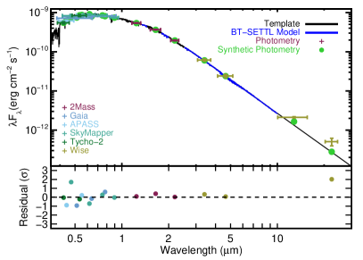
Figure 4: Best-fit spectral template and Goodman spectrum (black) compared to the photometry of TOI 451. Blue regions are BT-SETTL models, used to fill in gaps or regions of high telluric contamination. Literature photometry is colored according to the source with horizontal errors corresponding to the filter width and vertical errors the measurement errors. Corresponding synthetic photometry is shown as green points. The bottom panel shows the residuals in terms of standard deviations from the fit, with a single point ($W1$) off the scale.

3.2 Infrared excess

The two reddest bands, $W3$ (12$\mu$m) and $W4$ (22$\mu$m) were both brighter than the derived from the best-fit template. We estimated an excess flux of $26\pm 7$% at $W3$, and $70\pm 30\%$ at $W4$ ($3.7$ and $2.3\sigma$, respectively, assuming Gaussian errors). This suggests a cool $\lesssim 300\,K$ debris disk. The $W2$ excess was not significant, both because of the large uncertainty in the $W4$ magnitude (8.63$\pm$0.29) and because the SED analysis is sensitive to the choice of template at long wavelengths.

The frequency of infrared excesses decreases with age, declining from tens of percent at ages less than a few hundred Myr to a few percent in the field (Meyer et al., 2008; Siegler et al., 2007; Carpenter et al., 2009). In the similarly-aged Pleiades cluster, Spitzer 24$\mu$m excesses are seen in 10% of FGK stars (Gorlova et al., 2006). This excess emission suggests the presence of a debris disk, in which planetesimals are continuously ground into dust (see Hughes et al., 2018, for a review).

3.2.1 Mass

To determine the mass of TOI 451, we used the MESA Isochrones and Stellar Tracks (MIST; Dotter, 2016; Choi et al., 2016). We compared all available photometry to the model-predicted values, accounting for errors in the photometric zero-points, reddening, and stellar variability. We restricted the comparison to stellar ages of 50–200 Myr and solar metallicity based on the properties of the stream. We assumed Gaussian errors on the magnitudes, but included a free parameter to describe underestimated uncertainties in the models or data. The best-fit parameters from the MIST models were $M_{*}=0.950\pm 0.020M_{\odot}$, $R_{*}=0.850\pm 0.015R_{\odot}$, $T_{\text{eff}}$$=5555\pm$45 K, and $L_{*}=0.610\pm 0.030L_{\odot}$. These were consistent with our other determinations, but we adopt our empirical $L_{*}$, $T_{\text{eff}}$ and $R_{*}$ estimates from the SED and only utilize the $M_{*}$ value from the evolutionary models in our analysis.

3.3 Radial velocities

We used high resolution optical spectra from SALT/HRS, NRES/LCO, and SMARTS/CHIRON to determine stellar radial velocities (RVs). We did not include Gaia because the RV zero-point has not been established in the same manner as our ground-based data.

We computed the spectral-line broadening functions (BFs; Rucinski, 1992; Tofflemire et al., 2019) through linear inversion of our spectra with a narrow-lined template. For the template, we used a synthetic PHOENIX model with $T_{\text{eff}}$ $=5400$ K and $\log{g}$  $=4.5$ (Husser et al., 2013). The BF accounts for the RV shift and line broadening. We computed the BF for each echelle order and combined them weighted by their S/N. We then fit a Gaussian profile to the combined BF to measure the RV. The RV uncertainty was determined from the standard deviation of the best-fit RV from three independent subsets of the echelle orders.

For HRS epochs, which consisted of three individual exposures, and the first NRES epoch, which consisted of two individual exposures, the RV and its uncertainty were determined from the error-weighted mean and standard error of the three individual spectra.

The resulting RVs are listed in Table 3. The RV zero-points were calculated from the spectra obtained in this work and Rizzuto et al. (2020) and are based on telluric features. The zero-points are: $0.05\pm 0.10$ for HRS (28 spectra), $0.32\pm 0.09$ for NRES (11 spectra), and $-0.05\pm 0.16$ for CHIRON (1 spectrum). The S/N was assessed at $\sim 6580\AA$.

Table 3: Radial velocity measurements of TOI 451

Site	BJD	RV	$\sigma_{RV}$	S/N
		(km s-1)	(km s-1)
HRS	2458690.652	19.8	0.1	80
HRS	2458705.606	19.7	0.1	86
HRS	2458709.606	19.8	0.1	70
HRS	2458713.584	19.9	0.1	60
HRS	2458752.482	20.04	0.03	83
HRS	2458760.468	20.0	0.2	74
NRES	2458695.868	20.20	0.09	13
NRES	2458699.850	20.3	0.1	7
CHIRON	2458529.560	20.00	0.06	24
Weighted mean: 19.9 (km/s)
RMS: 0.12 (km/s)
Std Error: 0.04 (km/s)

Note. — The zero-points are not included in the individual velocities but are accounted for in the statistics listed in the bottom rows. The zero-points are: $0.05\pm 0.10$ for HRS, $0.32\pm 0.09$ for NRES, and $-0.05\pm 0.16$ for CHIRON. The S/N was assessed at $\sim 6580\AA$. For the HRS and NRES epochs, which consist of multiple back-to-back spectra, the S/N for the middle spectrum is listed.

3.4 Orbit of TOI 451 and TOI 451 B

We used Linear Orbits for the Impatient via the python package lofti_gaiaDR2 (LOFTI; Pearce et al., 2020) to constrain the orbit of TOI 451 and TOI 451 B. Briefly, the lofti_gaiaDR2 retrieves observational constraints for the components from the Gaia archive and fits Keplerian orbital elements to the relative motion using the Orbits for the Impatient rejection sampling algorithm (Blunt et al., 2017). Unresolved binaries such as TOI 451 B can pose issues for LOFTI. While TOI 451 B’s $RUWE$ suggests binarity, it is still relatively low ($1.2$) and only on the edge of where astrometric accuracy compromises LOFTI (Pearce et al., 2020). We applied LOFTI to the system but caution that the unresolved binary may influence the results to an unknown, but likely small, degree. Our LOFTI fit constrained the orbit of TOI 451 and TOI 451 B to be close to edge-on: we found an orbital inclination of $i=93.8\pm 11.6^{\circ}$.

3.5 Stellar rotation

3.5.1 Projected rotation velocity

We used the high resolution CHIRON spectrum to measure the projected rotation velocity of TOI 451. We deconvolved the observed spectrum against a non-rotating synthetic spectral template from the ATLAS9 atmosphere models (Castelli & Kurucz, 2004) via a least-squares deconvolution (following Donati et al., 1997). We fitted the line profile with a convolution of components accounting for the rotational, macroturbulent, and instrumental broadening terms. The rotational kernel and the radial tangential macroturbulent kernels were computed as prescribed in Gray (2005), while the instrument broadening term was a Gaussian of FWHM $3.75$ $\rm km~{}s^{-1}$ set by the CHIRON resolution. We found a projected rotational broadening of $v\sin{i_{*}}=7.9\pm 0.5\,\rm km~{}s^{-1}$ and a macroturbulence of $2.2\pm 0.5\,\rm km~{}s^{-1}$ for TOI 451.

3.5.2 Rotation period

In WASP-South, each of the six seasons of data shows clear modulation at 5.2 days, with variations in phase and the amplitude varying from 0.01 to 0.023 (Figure 5). The mean period from WASP-South is 5.20 days and the standard deviation is 0.02.

We measured the stellar rotation period from the TESS data using Gaussian processes (GPs) (Angus et al., 2018) as implemented in celerite (Foreman-Mackey et al., 2017). We used the same rotation kernel as in Newton et al. (2019), which is composed of a mixture of two stochastically driven, damped harmonic oscillators. The primary signal is an oscillator at the stellar rotation period $P_{*}$. The secondary signal is at half the rotation period. We also included a jitter term. The parameters we fit for are described in detail in §5.1, where the GP was fit simultaneously with the transits. We used the period from WASP-South to place a wide prior on the GP fit (see §5.1). The period we measured from the GP is $\ln{P_{*}}=1.635^{+0.027}_{-0.024}$ or $5.1\pm 0.1$ d.

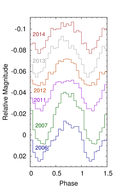
Figure 5: The WASP-South photometry from each year of observation, folded on the 5.2 d rotation period. For display purposes we have added magnitude and phase offsets.

3.5.3 Stellar inclination

We used the procedure outlined in Masuda & Winn (2020) to infer the inclination $i$ from $P_{*}$, $v\sin{i_{*}}$, $R_{*}$, and their respective errors. This implementation is accurate even in the case of large uncertainties on the rotation period and $v\sin{i_{*}}$. We used an affine invariant Markov Chain Monte Carlo sampler (Goodman & Weare, 2010) to determine the posterior probability distribution of $\cos{i_{*}}$. We explored the parameter space of $\cos{i_{*}}$, $R_{*}$, and $P_{*}$, comparing the $v\sin{i_{*}}$ derived from the fit parameters at each step to the measured $v\sin{i_{*}}$. We imposed Gaussian priors on $R_{*}$ and $P_{*}$ based on our measurements for the system, and a prior that $0\leq\cos{i_{*}}\leq 1$. We took the median and 68% confidence intervals as the best value and error. Adopting the convention that $i_{*}<90{\degree}$, $i_{*}=69^{+11}_{-8}{\degree}$. The $2\sigma$ confidence interval spans 56$\degree$ to 86$\degree$, so the stellar inclination is not inconsistent with alignment between the stellar spin axis, the planetary orbital axes, and the binary orbital axis.

4 Membership in Psc–Eri

In this section, we present evidence to support identification of TOI 451 as a member of Psc–Eri. While kinematics provide strong support, the stream membership is under active discussion in the literature, so here we consider other indicators of youth.

4.1 Kinematics

The original sample from Meingast et al. (2019) required RVs from Gaia for membership. Curtis et al. (2019) extended the sample to two dozen hotter stars by incorporating RVs from the literature. Recent searches have identified candidate Psc–Eri members without RVs. Röser & Schilbach (2020) adapted the convergent point method (van Leeuwen, 2009) to the highly elongated structure of the stream. After placing distance and tangential velocity constraints on stars in the vicinity of the Meingast et al. (2019) sample, they identified 1387 probable stream members. Ratzenböck et al. (2020) identified around 2000 new members with a machine learning classifier, trained on the originally identified sample of stream members. Röser & Schilbach (2020) calculated a bulk Galactic velocity for the Psc–Eri members identified by Meingast et al. (2019) of $(U,V,W)=(-8.84,-4.06,-18.33)\pm(2.2,1.3,1.7)$ km/s. This agrees with the value we have calculated for TOI 451 of $(-10.92,-4.18,-18.81)$ km/s within 1$\sigma$. Based on the space velocities and using the Bayesian membership selection of Rizzuto et al. (2011), we computed a Psc–Eri membership probability of 97% for TOI 451, and 84% for the companion TOI 451 B.

TOI 451 was included (as Gaia DR2 4844691297067063424) in the original membership list from Meingast et al. (2019) and in the subset with roxtation periods from TESS data identified by Curtis et al. (2019). It also was listed as a member in Ratzenböck et al. (2020) and Röser & Schilbach (2020).

4.2 Atmospheric Parameters and Abundances

We used the high-resolution (R$\sim$ 46,000) spectra obtained with the SALT telescope to derive stellar abundances, as well as $T_{\text{eff}}$ and $\log{g}$ . The spectra cover $\sim$3700–8900 Å. We median stacked the spectra to obtain a final spectrum with a S/N around 170 in the continuum at $\sim$5000 Å. We derived the $T_{\text{eff}}$, $\log{g}$ , [Fe/H] and the microturbulent velocity (v_micro) using the Brussels Automatic Code for Characterizing High accUracy Spectra (BACCHUS; Masseron et al., 2016) following the method detailed in Hawkins et al. (2020a). To summarize, we setup BACCHUS using the atomic line list from the fifth version of the Gaia-ESO linelist (Heiter et al., submitted) and molecular information for the following species were also included: CH (Masseron et al., 2014); CN, NH, OH, MgH and C₂ (T. Masseron, private communication); and SiH (Kurucz linelists). We employed the MARCS model atmosphere grid (Gustafsson et al., 2008), and the TURBOSPECTRUM (Plez, 2012) radiative transfer code. BACCHUS uses the standard Fe excitation-ionization balance technique to derive $T_{\text{eff}}$, $\log{g}$ , and [Fe/H]. We refer the reader to Section 3 of Hawkins et al. (2020b) for a more detailed description of BACCHUS. The stellar atmospheric parameters derived from Fe excitation-ionization balance are $T_{\text{eff}}$ $=5556\pm 60$, $\log{g}$  $=4.62\pm 0.17$ dex, [Fe/H] $=-0.02\pm 0.08$ dex. The $T_{\text{eff}}$ and implied $\log{g}$  derived from a simultaneous fit of the star’s spectral-energy-distribution are $T_{\text{eff}}$ $=5550\pm 56$, $\log{g}$  $=4.53\pm 0.04$. Encouragingly, these values are, within the uncertainties, consistent with the physical properties outlined in Table 2, which were determined without high-resolution spectra.

Once the stellar atmospheric parameters were determined, we determined the abundance of Li at 6708 Å, A(Li). The presence (or absence) of large amounts of Li is an age indicator. Li fuses at the relatively low temperature of 2.5 $\times 10^{6}$ K. As a star ages, Li mixes downward into regions hotter than this temperature, where it is burned into heavier elements. Therefore, the abundance of Li decreases as the star ages. The amount of depletion varies with mass (or $T_{\text{eff}}$, given a main sequence population). Therefore, A(Li) at a given $T_{\text{eff}}$ constrains a star’s age. This applies to both the Galactic disk (e.g. Ramírez et al., 2012) and open clusters (e.g. Boesgaard et al., 1998; Takeda et al., 2013; Martín et al., 2018; Bouvier et al., 2018).

To measure A(Li), we used the BACCHUS module abund. Using abund, we generated a set of synthetic spectra at 6708 Å with differing atmospheric abundances. We then used $\chi^{2}$ minimization to find the synthetic spectrum that best fits the observed spectrum. We determined A(Li) $=2.80\pm 0.10$ dex.

We compare A(Li) and $T_{\text{eff}}$ of TOI 451 to the observed trends in the Galactic Disk (Ramírez et al., 2012), the Pleiades (Bouvier et al., 2018), and the Hyades (Takeda et al., 2013) (Fig. 6). A(Li) for TOI 451 closely matches A(Li) for the Psc-Eri stream, indicating that it is likely $\sim$120 Myr old and a stream member.

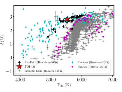
Figure 6: $T_{\text{eff}}$ as a function of the atmospheric abundance of Li, A(Li), for TOI 451 (red star), the Galactic Disk (gray circles; Ramírez et al., 2012), the Pleiades (cyan circles; Bouvier et al., 2018), the Hyades (magenta circles; Takeda et al., 2013), and the Psc–Eri stream (black circles; Hawkins et al., 2020a). TOI 451 has a measured Li abundance that is consistent with the Psc–Eri stream.

Figure 7: Rotation period as a function of color for TOI 451 and TOI 451 B (red stars), Psc-Eri members (black circles; Curtis et al., 2019), and Pleiades members (cyan circles; Rebull et al., 2016). Pleiades members are used to supplement the Psc-Eri members, which do not extend to later spectral types. Both TOI 451 and TOI 451 B have periods consistent with the color–rotation sequence that describes a $\sim 120$ Myr old cluster.

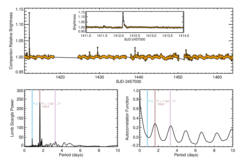
Figure 8: Top: TESS light curve of TOI 451 B. The inset shows additional detail of a large flare detected in the light curve. Typical error bars are about 0.002, smaller than the data points on the scale shown here. Bottom: Lomb Scargle periodogram (Left) and autocorrelation function (right) of the TESS light curve. Both the periodogram and autocorrelation function show a clear signal at 1.64 days. The true amplitude of the flares and signals in this light curve are larger than shown here due to diluting flux from TOI 451.

4.3 Rotation period of TOI 451

As described in §3.5, we measured a rotation period of $5.1\pm 0.1$ d, consistent with the 5.02 days reported in Curtis et al. (2019). As discussed in that work, this places TOI 451 on the slow sequence, the rotation–color sequence to which the initial distribution of periods converges for a uniform-age population. Figure 7 places TOI 451 in the context of other members of Psc-Eri and Pleiades cluster members.

4.4 Rotation period of TOI 451 B

We extracted a light curve of TOI 451 B from the TESS 30 minute full frame images (the light curve would be from the composite object if TOI 451 B is itself a binary). TOI 451 and its companion(s) are only separated by 37 arcseconds, or about two TESS pixels, so the images of these two stars overlap substantially on the detector. The light curve of the companion TOI 451 B is clearly contaminated by the 14x brighter primary star. We therefore took a non-standard approach to extracting a light curve for the companion. We started with the flux time series of the single pixel closest to the position of TOI 451 B during the TESS observations, clipped out exposures with flags indicating low-quality datapoints and between times $1419<BJD-2457000<1424$ (when a heater onboard the spacecraft was activated), and divided by the median flux value to normalize the light curve. We removed systematics and contaminating signals from TOI 451 by decorrelating the single-pixel light curve of TOI 451 B with mean and standard deviation quaternion time series (see Vanderburg et al., 2019), a fourth order polynomial, and the flux from the pixel centered on TOI 451 (to model and remove any signals from the primary star). The resulting light curve, shown in Figure 8 shows several flares and a clear rotation signal. Before calculating rotation period metrics, we clipped out flares and removed points with times $1449<BJD-2457000<1454$, which showed some residuals systematic effects.

We measured the companion’s rotation period by calculating the Lomb-Scargle periodogram and autocorrelation function from the two-sector TESS light curve. The ACF and Lomb-Scargle periodogram both showed a clear detection of a 1.64 day rotation period, though we cannot completely rule out the possibility that TOI 451 B’s rotation period is actually an integer multiple of this period.

We note that Rebull et al. (2016), in their analysis of the Pleiades, detect periods for 92% of the members, and suggest the remaining non-detections are due to non-astrophysical effects. We have suggested TOI 451 B is a binary, which we might expect to manifest as two periodicities in the lightcurve. We only detect one period in our lightcurve; however, a second signal could have been impacted by systematics removal or be present at smaller amplitude than the 1.64 day signal, and so we do not interpret the lack of a second period further.

At around 100 Myr, stars of this type (early to mid M dwarfs) are in the midst of converging to the slow sequence. They may have a range of rotation periods, but are generally rotating with periods of a few days (Rebull et al., 2016). While the Psc-Eri members studied in Curtis et al. (2019) do not extend to stars as low mass as TOI 451 B, we can consider the similarly-aged Pleiades members as a proxy. Figure 7 demonstrates that the $1.64$ day rotation period of TOI 451 B is typical for stars of its color at $120$ Myr.

4.5 Age Diagnostics from GALEX NUV Fluxes

Chromospheric and coronal activity depend on stellar rotation and are thus also an age indicator (e.g. Skumanich, 1972). We use excess UV emission as an age diagnostic for TOI 451 and TOI 451 B, considering the flux ratio $F_{NUV}/F_{J}$ as a function of spectral type. The use of this ratio for this purpose was suggested by Shkolnik et al. (2011). More details on this general technique and applications to the Psc-Eri stream are provided in Appendix A.

TOI 451 and TOI 451 B both were detected by GALEX  during short NUV exposures taken for the All-Sky Imaging Survey (AIS, Bianchi et al. 2017). Both stars were also observed with longer NUV exposures for the Medium-depth Imaging Survey (MIS), but only the primary’s brightness was reported ($m_{nuv,p}=16.674\pm 0.006$ mag). Using the MIS data, we measured the secondary’s brightness to be $m_{nuv,s}=21.33\pm 0.06$ mag (see Appendix A for details).

In Figure 9, we plot $F_{NUV}/F_{J}$ versus spectral type for TOI 451 and TOI 451 B. Since both spectral type and color should be unaffected by a near-equal mass unresolved companion, the fact that TOI 451 B is a binary is not expected to impact this analysis. We also show isochronal sequences for the other members of Psc-Eri and the similarly-aged Pleiades cluster, using the latter to define the M dwarf regime at this age. To illustrate the expected fluxes for older stars, we show the sequence for the Hyades cluster. Details on the derivations of these isochronal sequences are given in Appendix A.

While solar-type stars only have excess NUV and X-ray fluxes for a short time, the NUV flux of early M dwarfs remains saturated to ages $\lesssim 300$ Myr before sharply declining (Shkolnik & Barman, 2014). TOI 451 is consistent with the sequences for other G-dwarfs in all three clusters: as expected its UV excess is not a highly discriminating age diagnostic. However, the wide companion TOI 451 B sits above the Hyades sequence, and shows an NUV flux excess that is broadly consistent with the Pleiades sequence that is similar in age to Psc–Eri. This supports the membership of the TOI 451 system to the Psc-Eri stream.

Figure 9: GALEX NUV/NIR flux ratio ($F_{NUV}/F_{J}$ as a function of spectral type for TOI 451 and TOI 451 B, as well as several stellar populations spanning the age range where NUV fluxes are diagnostic of age. To allow direct comparison to other definitions of this youth diagnostic, we also show the $m_{nuv}-m_{J}$ and $B_{p}-R_{p}$ colors. The dashed lines show the detection limits for each cluster shown; objects lying to the lower right would not have been detected in GALEX AIS at the assumed distance to that cluster (targeted pointings, e.g. for many Pleiades targets, extend deeper).

5 Analysis

5.1 Transit model

We modeled the transit with misttborn (Mann et al., 2016; Johnson et al., 2018). This routine uses batman (Kreidberg, 2015) to produce the transit model of Mandel & Agol (2002) and explores the posterior with the Markov Chain Monte Carlo sampler emcee (Foreman-Mackey et al., 2013).

To model the transits of each of the three planets, we fitted for the planet-to-star radius ratio $R_{P}/R_{*}$, impact parameter $b$, period $P$, and the epoch of the transit midpoint $T_{0}$. We assumed $R_{P}/R_{*}$ is the same in all filters. We also fitted for the mean stellar density ($\rho_{*}/\rho_{\odot}$). We used a quadratic limb-darkening law described by $g_{1,f}$ and $g_{2,f}$ for each filter $f$. This is a reasonable choice given that the host star is Sun-like (Espinoza & Jordán, 2016). We fitted the limb darkening parameters using the Kipping (2013) parameterization ($q_{1,f}$, $q_{2,f}$). For our first fit, we fixed the eccentricity $e$ to $0$. For our second fit, we allowed $e$ and the argument of periastron $\omega$ to vary, using the parameterization $\sqrt{e}\sin{\omega}$ and $\sqrt{e}\cos{\omega}$ (Ford, 2006; Eastman et al., 2013).

We used uniform priors for the planetary parameters, and a Gaussian prior on $\rho_{*}/\rho_{\odot}$ centered at 1.34 (Table 2) with a $1\sigma$ width of 0.5. We placed Gaussian priors on the limb-darkening parameters based on theoretical values for a star with the temperature and radius given in Table 2. We assume solar metallicity based on the mean iron abundance of the Psc-Eri members studied by Hawkins et al. (2020a), who found $\rm{[Fe/H]}=-0.03$ dex with a dispersion of $0.04$-$0.07$ dex. For the Gaussian means of the limb darkening priors, we use the coefficients calculated with the Limb Darkening Toolkit (Parviainen & Aigrain, 2015, ; LDTK), using the filter transmission curves available for LCO $z_{s}$ and TESS. The PEST bandpass is similar to that of MEarth, and following Dittmann et al. (2017), we adopted the filter profile from Dittmann et al. (2016). For Spitzer, we used the tabulated results from Claret & Bloemen (2011). Due to systematic uncertainties in limb-darkening parameters (Müller et al., 2013; Espinoza & Jordán, 2015), the potential impact of spots (Csizmadia et al., 2013) and differences between LDTK and Claret coefficients, we used 0.1 for the $1\sigma$ width of the priors on $q$.

For stellar rotation, we used the Gaussian process model of a mixture of simple harmonic oscillators introduced in §3.5, with the parameters sampled in log-space (in the following, logarithms are all natural logarithms). The model includes the power at the rotation period $P_{*}$ (the primary signal) and at $P_{*}/2$ (the secondary signal). We fitted for the period of the primary signal $\ln{P_{*}}$, the amplitude of the primary signal $\ln{A_{1}}$, the relative amplitudes of the primary and secondary signals $m$ (where $A_{1}/A_{2}=1+e^{-m}$), the decay timescale (or “quality factor”) of the secondary signal $\ln{Q_{2}}$, and the difference in quality factors $\ln{\Delta Q}$ (where $\ln{\Delta Q}=\ln\left(Q_{1}-Q_{2}\right)$). We additionally included a photometric jitter term, $\sigma_{\mathrm{GP}}$.

We placed a Gaussian prior on $\ln{P_{\rm*}}$ centered at $1.6487$, based on the period from the WASP data, with a width of $0.05$. We use log-normal priors on the remaining parameters. We require $\ln{\Delta Q}>0$ to ensure that the primary signal has higher quality than the secondary, and $\ln{Q_{2}}>\ln{0.5}$ since we are modeling a signal with periodic behavior (cf. Equation 23 and Figure 1 in Foreman-Mackey et al. 2017).

The GP model was applied to data from TESS, LCO, and PEST, but not data from Spitzer. The latter was assumed to have no out-of-transit variability remaining after the corrections described in §2.

The autocorrelation length of our $e=0$ fit was 470 steps, and for our variable-eccentricity fit was 1200 steps. We ran the MCMC chain for 100 times the autocorrelation times with 100 walkers, discarding the first half as burn-in. Figures 1 and 2 shows the best-fitting models overlain on the data, and Table 4 lists the median and 68% confidence limits of the fitted planetary and stellar parameters.

Table 4: Transit fitting results for the TOI 451 system

Parameter	Planet b	Planet c	Planet d	Planet b	Planet c	Planet d
	$e$,$\omega$ fixed			$e$,$\omega$ free
Fitted Transit Parameters
$T_{0}$ (BJD)	$1410.9900^{+0.0056}_{-0.0037}$	$1411.7956^{+0.0048}_{-0.0026}$	$1416.63478^{+0.00088}_{-0.00092}$	$1410.9909^{+0.0046}_{-0.0042}$	$1411.7961^{+0.0039}_{-0.0030}$	$1416.63499^{+0.00097}_{-0.00093}$
$P$ (days)	$1.858703^{+2.5\times 10^{-5}}_{-3.5\times 10^{-5}}$	$9.192522^{+6.0\times 10^{-5}}_{-10\times 10^{-5}}$	$16.364988\pm 4.4\times 10^{-5}$	$1.858701^{+2.7\times 10^{-5}}_{-3.3\times 10^{-5}}$	$9.192523^{+6.4\times 10^{-5}}_{-8.4\times 10^{-5}}$	$16.364981^{+4.7\times 10^{-5}}_{-4.9\times 10^{-5}}$
$R_{P}/R_{\star}$	$0.0199^{+0.0010}_{-0.0011}$	$0.03237^{+0.00065}_{-0.00070}$	$0.04246\pm 0.00044$	$0.0203^{+0.0014}_{-0.0011}$	$0.03206^{+0.00090}_{-0.00085}$	$0.04205^{+0.00050}_{-0.00045}$
$b$	$0.22^{+0.20}_{-0.15}$	$0.139^{+0.121}_{-0.096}$	$0.387^{+0.047}_{-0.039}$	$0.42^{+0.32}_{-0.28}$	$0.52^{+0.23}_{-0.32}$	$0.23^{+0.18}_{-0.16}$
$\rho_{\star}$ ($\rho_{\odot}$)	$1.294^{+0.061}_{-0.088}$			$1.41^{+0.15}_{-0.16}$
$q_{1,1}$	$0.344^{+0.080}_{-0.078}$			$0.385^{+0.083}_{-0.084}$
$q_{2,1}$	$0.394^{+0.068}_{-0.082}$			$0.391^{+0.070}_{-0.088}$
$q_{1,2}$	$0.325^{+0.095}_{-0.096}$			$0.325^{+0.099}_{-0.086}$
$q_{2,2}$	$0.365^{+0.080}_{-0.096}$			$0.364^{+0.082}_{-0.100}$
$q_{1,3}$	$0.058^{+0.076}_{-0.045}$			$0.058^{+0.080}_{-0.045}$
$q_{2,3}$	$0.341^{+0.085}_{-0.094}$			$0.324^{+0.089}_{-0.092}$
$q_{1,4}$	$0.036^{+0.042}_{-0.025}$			$0.027^{+0.038}_{-0.020}$
$q_{2,4}$	$0.155^{+0.094}_{-0.086}$			$0.159^{+0.095}_{-0.090}$
$\sqrt{e}\sin\omega$	$\cdots$			$-0.23^{+0.19}_{-0.21}$	$-0.26^{+0.16}_{-0.19}$	$0.02^{+0.11}_{-0.13}$
$\sqrt{e}\cos\omega$	$\cdots$			$-0.09^{+0.42}_{-0.38}$	$0.01^{+0.36}_{-0.43}$	$-0.01^{+0.32}_{-0.29}$
Fitted Gaussian Process Parameters
$\log{P_{\mathrm{GP}}}$ (day)	$1.636^{+0.027}_{-0.024}$			$1.637^{+0.027}_{-0.024}$
$\log{A_{\mathrm{GP}}}$ (%2)	$-12.08^{+0.36}_{-0.26}$			$-12.1^{+0.32}_{-0.25}$
$\log{Q1_{\mathrm{GP}}}$	$1.62^{+0.93}_{-0.94}$			$1.59^{+0.89}_{-0.95}$
$\log{Q2_{\mathrm{GP}}}$	$1.25^{+0.33}_{-0.29}$			$1.25^{+0.34}_{-0.30}$
MixQ1,Q2	$4.6\pm 3.5$			$4.8^{+3.6}_{-3.2}$
$\sigma_{\mathrm{GP}}$ (%)	$-15.0^{+3.1}_{-3.4}$			$-15.0^{+3.1}_{-3.3}$
Derived Transit Parameters
$a/R_{\star}$	$6.93^{+0.11}_{-0.16}$	$20.12^{+0.31}_{-0.47}$	$29.56^{+0.46}_{-0.69}$	$6.63^{+0.51}_{-0.89}$	$18.9^{+1.4}_{-2.2}$	$30.69^{+0.82}_{-1.0}$
$i$ (∘)	$88.2^{+1.2}_{-1.7}$	$89.61^{+0.27}_{-0.36}$	$89.25^{+0.084}_{-0.1}$	$86.5^{+2.3}_{-2.9}$	$88.49^{+0.95}_{-0.67}$	$89.56^{+0.31}_{-0.35}$
$\delta$ (%)	$0.0396^{+0.0041}_{-0.0042}$	$0.1048^{+0.0043}_{-0.0045}$	$0.1803\pm 0.0037$	$0.0412^{+0.0059}_{-0.0043}$	$0.1028^{+0.0059}_{-0.0054}$	$0.1768^{+0.0042}_{-0.0038}$
$T_{14}$ (days)	$0.0849^{+0.0024}_{-0.0054}$	$0.1483\pm 0.0016$	$0.1707\pm 0.001$	$0.082^{+0.02}_{-0.017}$	$0.137^{+0.028}_{-0.031}$	$0.171^{+0.018}_{-0.017}$
$T_{23}$ (days)	$0.0815^{+0.0024}_{-0.0058}$	$0.1387^{+0.0015}_{-0.0016}$	$0.1543\pm 0.0011$	$0.078^{+0.019}_{-0.018}$	$0.125^{+0.026}_{-0.032}$	$0.156^{+0.016}_{-0.017}$
FPP parameter	$0.119^{+0.308}_{-0.094}$	$0.044^{+0.11}_{-0.038}$	$0.354^{+0.101}_{-0.072}$	$0.44^{+1.32}_{-0.38}$	$0.7^{+1.12}_{-0.61}$	$0.12^{+0.28}_{-0.11}$
$T_{\mathrm{peri}}$ (BJD)	$1410.99^{+0.0056}_{-0.0037}$	$1411.7956^{+0.0048}_{-0.0026}$	$1416.63478^{+0.00088}_{-0.00092}$	$1411.26^{+0.39}_{-0.89}$	$1410.4^{+4.6}_{-2.1}$	$1416.8^{+3.3}_{-3.8}$
$g_{1,1}$	$0.452^{+0.093}_{-0.100}$			$0.479^{+0.094}_{-0.100}$
$g_{2,1}$	$0.122^{+0.100}_{-0.078}$			$0.132^{+0.113}_{-0.086}$
$g_{1,2}$	$0.40\pm 0.12$			$0.41^{+0.12}_{-0.13}$
$g_{2,2}$	$0.148^{+0.116}_{-0.089}$			$0.154^{+0.111}_{-0.095}$
$g_{1,3}$	$0.151^{+0.093}_{-0.080}$			$0.145^{+0.090}_{-0.077}$
$g_{2,3}$	$0.067^{+0.082}_{-0.047}$			$0.075^{+0.083}_{-0.050}$
$g_{1,4}$	$0.052^{+0.048}_{-0.033}$			$0.046^{+0.045}_{-0.029}$
$g_{2,4}$	$0.122^{+0.081}_{-0.061}$			$0.106^{+0.080}_{-0.057}$
$R_{P}$ ($R_{\oplus}$)	$1.91\pm 0.12$	$3.1\pm 0.13$	$4.07\pm 0.15$	$1.94^{+0.15}_{-0.13}$	$3.07\pm 0.14$	$4.03\pm 0.15$
$a$ (AU)	$0.0283^{+0.0011}_{-0.0012}$	$0.0823^{+0.0033}_{-0.0036}$	$0.1208^{+0.0048}_{-0.0052}$	$0.0271^{+0.0023}_{-0.0038}$	$0.0771^{+0.0066}_{-0.0093}$	$0.1255^{+0.0057}_{-0.0065}$
$T_{\mathrm{eq}}$ (K)	$1491^{+23}_{-19}$	$875^{+13}_{-11}$	$722^{+11}_{-9}$	$1524^{+100}_{-60}$	$903^{+53}_{-36}$	$708^{+15}_{-12}$
$e$	$\cdots$			$0.19^{+0.20}_{-0.14}$	$0.2^{+0.18}_{-0.14}$	$0.057^{+0.133}_{-0.040}$
$\omega$ (∘)	$\cdots$			$238^{+85}_{-48}$	$266\pm 63$	$170^{+170}_{-120}$

Note. — $T_{\mathrm{eq}}$ assumes an albedo of 0 (the planets reflect no light) with no uncertainty. The planetary radii listed above are from the joint fit of TESS, ground-based, and Spitzer data. For the TESS-only fit, $R_{P}/R_{\star}$ for planets b, c and d, respectively are: $0.0194\pm 0.0011$, $0.0286\pm 0.0016$, and $0.0418^{+0.0012}_{-0.0013}$. The largest difference is for c. For the Spitzer-only fit of c, $R_{P}/R_{\star}=0.034\pm 0.001$. We suggest adopting the $e=0$ fit since the eccentricities from the variable-eccentricity fit are consistent with 0.

5.2 Additional investigations into the transit parameters

We performed fits of the TESS data using EXOFASTv2 (Eastman et al., 2019) software package, which simultaneously fits the transits with the stellar parameters. We first removed the stellar variability using the GP model described in Section 3.5, masking the transit prior to fitting. The stellar parameters were constrained by the spectral energy distribution (SED) and MESA Isochrones and Stellar Tracks (MIST) stellar evolution models Dotter (2016); Choi et al. (2016). We enforced Gaussian priors on $T_{\mathrm{eff}}$, [Fe/H], and $\log{g}$ following Section 3, and on the Gaia DR2 parallax corrected for a systematic offset (Stassun & Torres, 2018). We used a Gaussian prior on age of $125\pm 15$ Myr, and restricted extinction to $<0.039$ (Schlafly & Finkbeiner, 2011). The stellar parameters from EXOFASTv2 are: $T_{\text{eff}}=5563\pm 44K$, $M_{*}=0.94\pm 0.025$ and $R_{*}=0.834\pm 0.01$. We generally found excellent agreement with the best-fitting planetary parameters from misttborn.

We also fitted the TESS and Spitzer data sets independently. There is a $2\sigma$ discrepancy between the Spitzer transit depths of TOI 451 c ($R_{P}/R_{\star}=0.034\pm 0.001$) and the TESS transit depth ($R_{P}/R_{\star}=0.029\pm 0.002$). No significant differences are seen in the transit depths of TOI 451 d, which we might expect if there was dilution in the TESS data. The mildly larger planetary radius for TOI 451 c measured at $4.5\micron$ relative to that measured at TESS’s red-optical bandpass could be due to occulted starspots, unocculted plages, or atmospheric features. Given that the transits of c and d were observed at similar times, we might also expect differences in the depths of TOI 451 d if starspots caused the discrepancy for c; however, the nature of starspots (size, temperature, location/active latitudes, longevity) is not well-understood. Alternatively, the difference in transit depths for TOI 451 c could derive from its atmosphere. It is likely, however, that difference arises from systematics in the Spitzer data, as discussed in §2.1.2.

5.3 False positive analysis

We considered four different false-positive scenarios for each of the candidate planets: 1) there is uncorrected stellar variability, 2) TOI 451 is an eclipsing binary, 3) TOI 451 is a hierarchical eclipsing system, 4) there is a background or foreground eclipsing system. Relevant to the blend scenarios, transits are visible in the Spitzer data even when shrinking or shifting the aperture, indicating that the signal lands within 2 Spitzer pixels (2.4″) of TOI 451. Speckle imaging and Gaia RUWE rule out companions brighter than these limits (i.e., bright enough to cause the transits) down to $0.2\arcsec$, so a very close blend is required.

We ruled out stellar variability for all three planets from the Spitzer transits. For any spot contrast, stellar variation due to rotation and spots/plages will always be weaker at Spitzer wavelengths compared to TESS. For TOI 451, out-of-transit data taken by Spitzer shows a factor of $\simeq$4 lower variability than the equivalent baseline in TESS data. Thus, if any transit was due purely to uncorrected stellar variation, the shape, duration, and depth would be significantly different or the entire transit would not present in the Spitzer photometry.

We used the source brightness parameter from Vanderburg et al. (2019) to constrain the magnitude a putative blended source (bound or otherwise). The parameter, $\Delta m$, relates the ingress or egress duration to transit duration and reflects the true radius ratio, independent of whether there is contaminating flux: $\Delta m\leq 2.5\log_{10}(T^{2}_{12}/T^{2}_{13}/\delta)$. Here, $\delta$ is the transit depth, $T_{12}$ is the ingress/egress duration and $T_{13}$ the time between the first and third contact. We calculated $\Delta m$ for the posterior samples for our variable-eccentricity transit fit, and took the 99.7% confidence limit. We find $\Delta m<4.6$, $2.0$, $1.0$ for TOI 451 b, c and d, respectively.

Using the brightness constraints from our imaging data and the $\Delta m$ parameter, we statistically rejected the scenario where any of the transits are due to an unassociated field star, either an eclipsing binary or an unassociated transiting planetary system (Morton & Johnson, 2011). We drew information on every star within 1 degree of TOI 451 from Gaia DR2 satisfying the most conservative brightness limits ($\Delta T<4.6$). This yielded a source density of $\simeq$3500 stars per square degree, suggesting a negligible $\simeq 7\times 10^{-5}$ field stars that were missed by our speckle data and still bright enough to produce the candidate transit associated with b. Constraints are stronger for the other planets.

To investigate scenarios including a bound companion blended with the source, we first considered the constraint placed by the multi-wavelength transit depths. As explained in Désert et al. (2015), if the transit signals were associated with another star in the aperture, the transit depth observed by Spitzer would be deeper than that observed by TESS, owing to the decreased contrast ratio between the target and the blended star (which must be fainter as is assumed to be cooler) at 4.5$\mu$m compared to 0.75$\mu$m. Thus, the ratio of the Spitzer-to-TESS transit depths ($\delta S/\delta T$) provides a range of possible TESS-Spitzer colors of the putative companion ($C_{TS,\rm{comp}}$) in terms of the combined (unresolved) color ($C_{TS,\rm{combined}}$). Following Tofflemire et al. (in prep), we used the 95-percentile range for $\delta S/\delta T$ for each transit to derive the putative companion color:

$$C_{TS,\rm{comp}}<C_{TS,\rm{combined}}+2.5\log_{10}(\frac{\delta S}{\delta T}).$$ (1)

Adopting the weakest constraints from the three planets gives a $C_{TS,\rm{comp}}$ between 1.09 and 1.30 magnitudes, indicating that the putative bound companion must be similar in color to the target star.

We then simulated binary systems following Wood et al. (in prep) which we compared to the observational data and constraints. In short, we generated 5 million binaries following the period and mass ratio from Raghavan et al. (2010) and the eccentricity distribution from Price-Whelan et al. (2020). For each binary, we calculated the expected radial velocity curve, magnitude, and projected separation at the epoch of the speckle data. We then compared the generated models for a given simulated binary to our radial velocities, speckle data, and Gaia imaging and astrometry (Section 2.6.2). To account for stellar variability, we added 50 m s^-1 error to the velocity measurements. Binaries were then rejected based on the probability of the observational constraints being consistent with the binary star parameters by chance (color, source brightness, radial velocities, and all imaging/photometric data). We ran two versions of this simulation, one where a single companion was forced to eclipse the primary (for ruling out eclipsing binaries), and one where the binary’s orbital inclination was unrestricted (for hierarchical systems). The former set ruled out all non-planetary signals at periods matching any of the three planets (Figure 10). In the latter simulation, less than 0.01% of the simulated blends passed all observational constraints for the signals associated with any of the three planets.

We now take into consideration the probability that any given star happens to be an eclipsing binary (about 1%; Kirk et al. 2016), compared to the probability of a transiting planet (also about 1%; Thompson et al. 2018). The chance alignment of unassociated field stars is therefore $7\times 10^{-5}$ times as likely as the transiting planet scenario, and the hierarchical triple $1\times 10^{-4}$ times as likely. The probability of the host star itself being an eclipsing binary is negligible. The transiting planet hypothesis is significantly more likely than the non-transiting planet hypothesis, with a false positive probability of about $2\times 10^{-4}$. The probability of a star hosting a planet discovered by TESS is likely lower (about 0.05% based on current search statistics; Guerrero submitted) than assumed here. On the other hand, studies of the Kepler multi-planet systems indicate that the false positive rate for systems with two or more transiting planets is low (Lissauer et al., 2012, 2014), about a factor of 15 less for TESS planets (Guerrero, submitted), which would more than compensate for our assumption. The false positive probability of $2\times 10^{-4}$ is therefore an overestimate.

We have ruled out instrumental variability, chance alignment of unassociated field stars (including both eclipsing binaries and planetary systems), and bound eclipsing binaries or heirarchical triples, and therefore reject the false positives identified at the beginning of this section. We consider all three planets validated at high confidence.

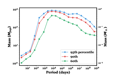
Figure 10: Distribution of surviving binaries from our false-positive simulation. In this case, the companion is forced to eclipse the star, as would be required to produce a transit-like signal. The curve rules out all stellar and brown dwarf companions at periods matching the three planets.

6 Summary and discussion

TOI 451 b, c and d are hot planets in close orbits around a young, Sun-like star. The inner planet, TOI 451 b, has a period of $1.9$ days and a radius of $1.9$$R_{\earth}$. This places it within or below the radius valley as defined in Van Eylen et al. (2018, cf. their Figure 6), although there are very few larger planets ($2-4$$R_{\earth}$) at such short orbital periods. At $3.1$ and $4.1$$R_{\earth}$, the outer two planets sit well above the radius valley. Since they are young and hot ($T_{\mathrm{eq}}=720$ to $1500$ K assuming $0$ albedo) and could be low-mass, their observed radii may be impacted by high-altitude hazes (Gao & Zhang, 2019).

At $120$ Myr, the solar-mass host star has completed the most magnetically active part of its lifetime and the era of strongest photoevaporative mass loss is expected to be complete (Owen & Wu, 2017). However, Rogers & Owen (2020) showed that overall photoevaporatively-driven radius evolution of a synthetic population was not complete until around 1 Gyr. Core-powered mass loss (Ginzburg et al., 2018) would be expected to shape planetary radii on timescales of 1 Gyr (Gupta & Schlichting, 2020). Thus, these planets may still be undergoing observable atmospheric mass loss.

We estimated the planetary masses using the non-parameteric mass-radius relation from Ning et al. (2018), which is based on the full Kepler data set. This assumes these young planets obey the same mass-radius relation as older stars, which may be inaccurate. We found masses for b, c, and d of $5^{+7}_{-3}$$M_{\oplus}$, $7^{+9}_{-4}$$M_{\oplus}$, and $8^{+11}_{-4}$$M_{\oplus}$, respectively. The expected RV amplitudes are about $2$ m/s for the three planets. Mass measurements of the planets are likely to be challenging due to the expected jitter and $5$ d stellar rotation period, but would provide valuable information on the planetary compositions.

Precise transit timing variations have the potential to yield measurement of the masses of the outer two planets. To estimate the TTV amplitudes, we assumed no other planets interact dynamically with the three we observe and used TTV2Fast2Furious (Hadden 2019; see Hadden et al. 2019). We estimated TTV amplitudes (measured peak to zero) of 2 min for TOI 451 c and d using our variable-eccentricity fit, or 30 sec for c and 1 min for d for our $e=0$ fit. The periodicity is about 75 d. At present, CHEOPS (Broeg et al., 2013) is the photometric facility that can provide the highest-precision photometry for this system. Due to its Sun-Synchronous orbit, CHEOPS can monitor TOI 451 with at least 50% observation efficiency for approximately one month every year. We used the equations of Price & Rogers (2014) to estimate the uncertainty on the mid-transit time achievable with CHEOPS for TOI 451 c and d from their respective ingress and total transit durations. We assumed an exposure time of 30 s. We estimated the precision in the mid-transit to be 2 and 1.6 min per transit for TOI 451 c and d, respectively. For the variable-eccentricity fit results, TTV measurements for these two planets may thus be within reach.

Using the system parameters reported in this paper and the estimated planet masses listed above, along with the estimated uncertainties on all parameters, we estimated the Transmission Spectroscopy Metric (TSM; Kempton et al., 2018) for the three TOI 451 planets. S/N scales linearly with TSM for stars with $J>9$ ($J=9.6$ mag for TOI 451), with a scale factor of around $1.2$. For planets b, c, and d we find TSM $=36\pm 22$, $59\pm 35$, and $98\pm 57$, respectively. These fairly large uncertainties result from the as-yet unknown planet masses, but even accounting for the likely distribution of masses we find 95.4% (2$\sigma$) lower limits of TSM$>14$, $26$, and $44$, respectively. Planets d is likely to be among the best known planets in its class for transmission spectroscopy (cf. Table 11; Guo et al., 2020).

In summary, we have validated a three-planet system around TOI 451, a solar mass star in the 120-Myr Pisces-Eridanis stream. The planets were identified in TESS, and confirmed to occur around the target star with some of the final observations taken by Spitzer as well as ground-based photometry and spectroscopy. We confirmed that TOI 451 is a member of Psc-Eri by considering the kinematics and lithium abundance of TOI 451, and the rotation periods and NUV activity levels of both TOI 451 and its wide-binary companion TOI 451 B (Appendix A discusses the utility of NUV activity for identifying new low-mass members of Psc-Eri). The stellar rotation axis, the planetary orbits, and the binary orbit may all be aligned; and there is evidence for a debris disk. The synergy of all-sky, public datasets from Gaia and TESS first enabled the identification of this star as a young system with a well-constrained age, and then the discovery of its planets.

AWM was supported through NASA’s Astrophysics Data Analysis Program (80NSSC19K0583). This material is based upon work supported by the National Science Foundation Graduate Research Fellowship Program under Grant No. DGE-1650116 to PCT. KH has been partially supported by a TDA/Scialog (2018-2020) grant funded by the Research Corporation and a TDA/Scialog grant (2019-2021) funded by the Heising-Simons Foundation. KH also acknowledges support from the National Science Foundation grant AST-1907417 and from the Wootton Center for Astrophysical Plasma Properties funded under the United States Department of Energy collaborative agreement DE-NA0003843. D.D. acknowledges support from the TESS Guest Investigator Program grant 80NSSC19K1727 and NASA Exoplanet Research Program grant 18-2XRP18 2-0136. I.J.M.C. acknowledges support from the NSF through grant AST-1824644, and from NASA through Caltech/JPL grant RSA-1610091.

This work makes use of observations from the Las Cumbres Observatory (LCO) network. Some of the observations reported in this paper were obtained with the Southern African Large Telescope (SALT). This work has made use of data from the EuropeanSpace Agency (ESA) mission Gaia (https://www.cosmos.esa.int/gaia), processed by the Gaia Data Processing and Analysis Consortium (DPAC, https://www.cosmos.esa.int/web/gaia/dpac/consortium). Funding for the DPAC has been provided by national institutions, in particular the institutions participating in the Gaia Multilateral Agreement. Based in part on observations obtained at the Southern Astrophysical Research (SOAR) telescope, which is a joint project of the Ministério da Ciência, Tecnologia e Inovações do Brasil (MCTI/LNA), the US National Science Foundation’s NOIRLab, the University of North Carolina at Chapel Hill (UNC), and Michigan State University (MSU).

We acknowledge the use of public TESS Alert data from pipelines at the TESS Science Office and at the TESS Science Processing Operations Center. Resources supporting this work were provided by the NASA High-End Computing (HEC) Program through the NASA Advanced Supercomputing (NAS) Division at Ames Research Center for the production of the SPOC data products.

This paper includes data collected by the TESS mission, which are publicly available from the Mikulski Archive for Space Telescopes (MAST). Funding for the TESS mission is provided by NASA’s Science Mission directorate. This research has made use of the Exoplanet Follow-up Observation Program website, which is operated by the California Institute of Technology, under contract with the National Aeronautics and Space Administration under the Exoplanet Exploration Program.

Appendix A UV excess as a way to identify young stars in Psc–Eri

Chromospheric activity is indicative of stellar ages in a parallel to rotational periods. Fast-rotating stars are active stars, and this activity manifests in young stars via both spectral line emission (most notably Ca H&K and H$\alpha$; Wilson 1963; Feigelson & Kriss 1981) and excess emission in the ultraviolet and X-rays (e.g. Ku & Chanan, 1979). X-ray emission from the ROSAT All-Sky Survey was used for searches of nearby young populations (e.g. Walter et al., 1994; Wichmann et al., 1996; Torres et al., 2006). The better sensitivity of the GALEX ultraviolet space observatory opened up new opportunities (e.g. Findeisen & Hillenbrand, 2010; Shkolnik et al., 2011; Rodriguez et al., 2011).

UV flux measurements allow age-dating via a comparison of a star to the isochronal sequences of representative young populations. Solar-type stars only demonstrate elevated NUV and X-ray fluxes for a short time (e.g. Pizzolato et al., 2003), so activity measures are unlikely to be informative for earlier type stars at all but the youngest ages. However, Shkolnik & Barman (2014) found that the $NUV$ flux of early M dwarfs remains saturated to ages $\tau\lesssim 300$ Myr, before then steeply declining to field levels. Thus, we expect elevated NUV activity for late-type stars in Psc-Eri (including TOI 451 B; $T_{eff}\sim 3500$ K), but not early type stars (including TOI 451, $T_{eff}\sim 5500$ K).

We consider the UV/NIR flux ratio $F_{NUV}/F_{J}$ as a function of spectral type, as suggested by Shkolnik et al. (2011). A similar method was also suggested by Findeisen & Hillenbrand (2010) based on $m_{NUV}-m_{J}$ and $J-K$ colors, while Rodriguez et al. (2011) used $m_{NUV}-m_{V}$ and $m_{nuv}-m_{J}$.

TOI 451 and TOI 451 B were detected by GALEX during short NUV exposures as part of the All-Sky Imaging Survey (AIS). (Bianchi et al., 2017) reported $m_{nuv,p}=16.77\pm 0.02$ mag and $m_{nuv,s}=21.68\pm 0.31$ mag for TOI 451 and TOI 451 B, respectively. Both stars also are clearly present in longer NUV exposures from the Medium-depth Imaging Survey (MIS), but only TOI 451’s brightness was reported in the MIS catalog ($m_{nuv,p}=16.674\pm 0.006$ mag; Bianchi et al. 2017). Since the AIS magnitude for TOI 451 B was only measured with a significance of $3.5\sigma$, we determined a more precise magnitude for TOI 451 B using data from the MIS. We downloaded the MIS image of the TOI 451 system from the MAST GALEX archive and performed aperture photometry, using the recommended aperture sizes and aperture corrections from Morrissey et al. (2007). For TOI 451, we recovered a brightness similar to the MIS catalog value ($m_{nuv,p}=16.637\pm 0.006$ mag). We measured the secondary’s brightness to be $m_{nuv,s}=21.33\pm 0.06$ mag, which is consistent with the AIS value within $\sim 1\sigma$. In our analysis, we adopt the MIS catalog value for the primary and our MIS aperture photometry value for the secondary. We also use $J$ band photometry from 2MASS (Cutri et al., 2003) and $B_{p}$ and $R_{p}$ photometry from Gaia DR2 (Gaia Collaboration et al., 2018).

In Figure 9, we show isochronal sequences for the other members of Psc-Eri using the membership catalog from Curtis et al. (2019) and GALEX photometry from the AIS catalog (Bianchi et al., 2017). Since this sample did not extend to later spectral types, we supplement the Psc-Eri sequence with the similarly-aged Pleiades cluster ($\tau\sim 120$ Myr; Stauffer et al. 1998), which yields a more robust M-dwarf sequence due to its lower distance and more complete census (Gaia Collaboration et al., 2018). To further extend the Pleiades sequence beyond the limit of the AIS, we also queried the GALEX catalog at MAST for photometry of Pleiades members observed in MIS fields, as well as in GO programs previously reported by Browne et al. (2009) and Findeisen & Hillenbrand (2010). Finally, to define the expected fluxes for older stars, we show the sequence of AIS catalog photometry for the Hyades cluster ($\tau\sim 680$ Myr; see Gossage et al. 2018 and discussion therein) based on the cluster core population identified by Röser et al. (2019).

For all clusters, we convert $B_{p}-R_{p}$ colors to spectral types using the color-spectral type relations of Pecaut & Mamajek (2013), as updated by E. Mamajek on 20190322. We also display the mapping of spectral type to $B_{p}-R_{p}$ on the upper axis. TOI 451 is indeed consistent with the sequences for other G stars in all three clusters, and hence its NUV excess is not strongly diagnostic of age. On the other hand, the early M dwarf TOI 451 B sits well above the Hyades sequence, and is instead consistent with the Pleiades sequence.

The success in applying this method to TOI 451 suggests that NUV excess–especially given the wide availability of data from GALEX–is a promising route for further growing the low-mass census of Psc–Eri. Examination of Figure 9 suggests that this method is applicable from mid K to mid M dwarfs.

References

- Allard et al. (2011) Allard, F., Homeier, D., & Freytag, B. 2011, in Astronomical Society of the Pacific Conference Series, Vol. 448, 16th Cambridge Workshop on Cool Stars, Stellar Systems, and the Sun, ed. C. Johns-Krull, M. K. Browning, & A. A. West, 91
- Angus et al. (2018) Angus, R., Morton, T., Aigrain, S., Foreman-Mackey, D., & Rajpaul, V. 2018, Monthly Notices of the Royal Astronomical Society, 474, 2094, doi: 10.1093/mnras/stx2109
- Arancibia-Silva et al. (2020) Arancibia-Silva, J., Bouvier, J., Bayo, A., et al. 2020, arXiv:2002.10556 [astro-ph]. https://arxiv.org/abs/2002.10556
- Astropy Collaboration et al. (2013) Astropy Collaboration, Robitaille, T. P., Tollerud, E. J., et al. 2013, A&A, 558, A33, doi: 10.1051/0004-6361/201322068
- Bailer-Jones et al. (2018) Bailer-Jones, C. A. L., Rybizki, J., Fouesneau, M., Mantelet, G., & Andrae, R. 2018, AJ, 156, 58, doi: 10.3847/1538-3881/aacb21
- Baraffe et al. (2015) Baraffe, I., Homeier, D., Allard, F., & Chabrier, G. 2015, A&A, 577, A42, doi: 10.1051/0004-6361/201425481
- Belokurov et al. (2020) Belokurov, V., Penoyre, Z., Oh, S., et al. 2020, arXiv e-prints, 2003, arXiv:2003.05467
- Benneke et al. (2019) Benneke, B., Wong, I., Piaulet, C., et al. 2019, The Astrophysical Journal Letters, 887, L14, doi: 10.3847/2041-8213/ab59dc
- Bianchi et al. (2017) Bianchi, L., Shiao, B., & Thilker, D. 2017, The Astrophysical Journal Supplement Series, 230, 24, doi: 10.3847/1538-4365/aa7053
- Blackwell & Shallis (1977) Blackwell, D. E., & Shallis, M. J. 1977, MNRAS, 180, 177, doi: 10.1093/mnras/180.2.177
- Blunt et al. (2017) Blunt, S., Nielsen, E. L., De Rosa, R. J., et al. 2017, AJ, 153, 229, doi: 10.3847/1538-3881/aa6930
- Boesgaard et al. (1998) Boesgaard, A. M., Deliyannis, C. P., Stephens, A., & King, J. R. 1998, ApJ, 493, 206, doi: 10.1086/305089
- Bouma et al. (2019) Bouma, L. G., Hartman, J. D., Bhatti, W., Winn, J. N., & Bakos, G. Á. 2019, ApJS, 245, 13, doi: 10.3847/1538-4365/ab4a7e
- Bouvier et al. (2018) Bouvier, J., Barrado, D., Moraux, E., et al. 2018, A&A, 613, A63, doi: 10.1051/0004-6361/201731881
- Brandeker & Cataldi (2019) Brandeker, A., & Cataldi, G. 2019, Astronomy and Astrophysics, 621, A86, doi: 10.1051/0004-6361/201834321
- Broeg et al. (2013) Broeg, C., Fortier, A., Ehrenreich, D., et al. 2013, in European Physical Journal Web of Conferences, Vol. 47, European Physical Journal Web of Conferences, 03005, doi: 10.1051/epjconf/20134703005
- Brown et al. (2013) Brown, T. M., Baliber, N., Bianco, F. B., et al. 2013, Publications of the Astronomical Society of the Pacific, 125, 1031, doi: 10.1086/673168
- Browne et al. (2009) Browne, S. E., Welsh, B. Y., & Wheatley, J. 2009, Publications of the Astronomical Society of the Pacific, 121, 450, doi: 10.1086/599365
- Buckley et al. (2006) Buckley, D. A. H., Swart, G. P., & Meiring, J. G. 2006, 6267, 62670Z, doi: 10.1117/12.673750
- Campo et al. (2011) Campo, C. J., Harrington, J., Hardy, R. A., et al. 2011, ApJ, 727, 125, doi: 10.1088/0004-637X/727/2/125
- Carpenter et al. (2009) Carpenter, J. M., Bouwman, J., Mamajek, E. E., et al. 2009, ApJS, 181, 197, doi: 10.1088/0067-0049/181/1/197
- Castelli & Kurucz (2004) Castelli, F., & Kurucz, R. L. 2004, ArXiv Astrophysics e-prints
- Choi et al. (2016) Choi, J., Dotter, A., Conroy, C., et al. 2016, ApJ, 823, 102, doi: 10.3847/0004-637X/823/2/102
- Claret & Bloemen (2011) Claret, A., & Bloemen, S. 2011, Astronomy and Astrophysics, 529, A75, doi: 10.1051/0004-6361/201116451
- Clemens et al. (2004) Clemens, J. C., Crain, J. A., & Anderson, R. 2004, in Proc. SPIE, Vol. 5492, Ground-based Instrumentation for Astronomy, ed. A. F. M. Moorwood & M. Iye, 331–340, doi: 10.1117/12.550069
- Collins et al. (2017) Collins, K. A., Kielkopf, J. F., Stassun, K. G., & Hessman, F. V. 2017, AJ, 153, 77, doi: 10.3847/1538-3881/153/2/77
- Crause et al. (2014) Crause, L. A., Sharples, R. M., Bramall, D. G., et al. 2014, Ground-based and Airborne Instrumentation for Astronomy V, 9147, 91476T, doi: 10.1117/12.2055635
- Csizmadia et al. (2013) Csizmadia, S., Pasternacki, T., Dreyer, C., et al. 2013, Astronomy and Astrophysics, 549, A9, doi: 10.1051/0004-6361/201219888
- Cubillos et al. (2014) Cubillos, P., Harrington, J., Madhusudhan, N., et al. 2014, ApJ, 797, 42, doi: 10.1088/0004-637X/797/1/42
- Curtis et al. (2019) Curtis, J. L., Agüeros, M. A., Mamajek, E. E., Wright, J. T., & Cummings, J. D. 2019, The Astronomical Journal, 158, 77, doi: 10.3847/1538-3881/ab2899
- Cutri et al. (2003) Cutri, R. M., Skrutskie, M. F., van Dyk, S., et al. 2003, VizieR Online Data Catalog, 2246
- Dahm (2015) Dahm, S. E. 2015, ApJ, 813, 108, doi: 10.1088/0004-637X/813/2/108
- Deming et al. (2015) Deming, D., Knutson, H., Kammer, J., et al. 2015, Astrophysical Journal, 805, doi: 10.1088/0004-637X/805/2/132
- Désert et al. (2015) Désert, J.-M., Charbonneau, D., Torres, G., et al. 2015, ApJ, 804, 59
- Dittmann et al. (2016) Dittmann, J. A., Irwin, J. M., Charbonneau, D., & Newton, E. R. 2016, The Astrophysical Journal, 818, 153, doi: 10.3847/0004-637X/818/2/153
- Dittmann et al. (2017) Dittmann, J. A., Irwin, J. M., Charbonneau, D., et al. 2017, Nature, 544, 333, doi: 10.1038/nature22055
- Donati et al. (1997) Donati, J.-F., Semel, M., Carter, B. D., Rees, D. E., & Collier Cameron, A. 1997, MNRAS, 291, 658, doi: 10.1093/mnras/291.4.658
- Dotter (2016) Dotter, A. 2016, The Astrophysical Journal Supplement Series, 222, 8, doi: 10.3847/0067-0049/222/1/8
- Eastman et al. (2013) Eastman, J., Gaudi, B. S., & Agol, E. 2013, Publications of the Astronomical Society of the Pacific, 125, 83, doi: 10.1086/669497
- Eastman et al. (2019) Eastman, J. D., Rodriguez, J. E., Agol, E., et al. 2019, arXiv e-prints, arXiv:1907.09480. https://arxiv.org/abs/1907.09480
- Espinoza & Jordán (2015) Espinoza, N., & Jordán, A. 2015, Monthly Notices of the Royal Astronomical Society, 450, 1879, doi: 10.1093/mnras/stv744
- Espinoza & Jordán (2016) —. 2016, Monthly Notices of the Royal Astronomical Society, 457, 3573, doi: 10.1093/mnras/stw224
- Evans et al. (2018) Evans, D. W., Riello, M., De Angeli, F., et al. 2018, A&A, 616, A4, doi: 10.1051/0004-6361/201832756
- Fazio et al. (2004) Fazio, G. G., Hora, J. L., Allen, L. E., et al. 2004, The Astrophysical Journal Supplement Series, 154, 10, doi: 10.1086/422843
- Feigelson & Kriss (1981) Feigelson, E. D., & Kriss, G. A. 1981, The Astrophysical Journal Letters, 248, L35, doi: 10.1086/183618
- Findeisen & Hillenbrand (2010) Findeisen, K., & Hillenbrand, L. 2010, The Astronomical Journal, 139, 1338, doi: 10.1088/0004-6256/139/4/1338
- Ford (2006) Ford, E. B. 2006, The Astrophysical Journal, 642, 505, doi: 10.1086/500802
- Foreman-Mackey (2016) Foreman-Mackey, D. 2016, The Journal of Open Source Software
- Foreman-Mackey et al. (2017) Foreman-Mackey, D., Agol, E., Ambikasaran, S., & Angus, R. 2017, The Astronomical Journal, 154, 220, doi: 10.3847/1538-3881/aa9332
- Foreman-Mackey et al. (2019) Foreman-Mackey, D., Barentsen, G., & Barclay, T. 2019, dfm/exoplanet: exoplanet v0.1.5, doi: 10.5281/zenodo.2587222
- Foreman-Mackey et al. (2013) Foreman-Mackey, D., Hogg, D. W., Lang, D., & Goodman, J. 2013, Publications of the Astronomical Society of the Pacific, 125, 306, doi: 10.1086/670067
- Fraine et al. (2014) Fraine, J., Deming, D., Benneke, B., et al. 2014, Nature, Volume 513, Issue 7519, pp. 526-529 (2014)., 513, 526, doi: 10.1038/nature13785
- Fulton et al. (2017) Fulton, B. J., Petigura, E. A., Howard, A. W., et al. 2017, The Astronomical Journal, 154, 19, doi: 10.3847/1538-3881/aa80eb
- Gaia Collaboration et al. (2016) Gaia Collaboration, Prusti, T., de Bruijne, J. H. J., et al. 2016, Astronomy and Astrophysics, 595, A1, doi: 10.1051/0004-6361/201629272
- Gaia Collaboration et al. (2018) Gaia Collaboration, Brown, A. G. A., Vallenari, A., et al. 2018, Astronomy and Astrophysics, 616, A1, doi: 10.1051/0004-6361/201833051
- Gao & Zhang (2019) Gao, P., & Zhang, X. 2019, arXiv e-prints, 2001, arXiv:2001.00055
- Ginsburg et al. (2019) Ginsburg, A., Sipőcz, B. M., Brasseur, C. E., et al. 2019, AJ, 157, 98, doi: 10.3847/1538-3881/aafc33
- Ginzburg et al. (2018) Ginzburg, S., Schlichting, H. E., & Sari, R. 2018, Monthly Notices of the Royal Astronomical Society, 476, 759, doi: 10.1093/mnras/sty290
- Goodman & Weare (2010) Goodman, J., & Weare, J. 2010, COMM. APP. MATH. AND COMP. SCI, 5
- Gorlova et al. (2006) Gorlova, N., Rieke, G. H., Muzerolle, J., et al. 2006, ApJ, 649, 1028, doi: 10.1086/506373
- Gossage et al. (2018) Gossage, S., Conroy, C., Dotter, A., et al. 2018, The Astrophysical Journal, 863, 67, doi: 10.3847/1538-4357/aad0a0
- Gray (2005) Gray, D. F. 2005, The Observation and Analysis of Stellar Photospheres
- Guerrero (submitted) Guerrero. submitted
- Guo et al. (2020) Guo, X., Crossfield, I. J. M., Dragomir, D., et al. 2020, AJ, 159, 239, doi: 10.3847/1538-3881/ab8815
- Gupta & Schlichting (2019) Gupta, A., & Schlichting, H. E. 2019, Monthly Notices of the Royal Astronomical Society, 487, 24, doi: 10.1093/mnras/stz1230
- Gupta & Schlichting (2020) —. 2020, Monthly Notices of the Royal Astronomical Society, doi: 10.1093/mnras/staa315
- Gustafsson et al. (2008) Gustafsson, B., Edvardsson, B., Eriksson, K., et al. 2008, A&A, 486, 951, doi: 10.1051/0004-6361:200809724
- Hadden (2019) Hadden, S. 2019, Zenodo, doi: 10.5281/zenodo.3356829
- Hadden et al. (2019) Hadden, S., Barclay, T., Payne, M. J., & Holman, M. J. 2019, The Astronomical Journal, 158, 146, doi: 10.3847/1538-3881/ab384c
- Harris et al. (2020) Harris, C. R., Millman, K. J., van der Walt, S. J., et al. 2020, Nature, 585, 357, doi: 10.1038/s41586-020-2649-2
- Hawkins et al. (2020a) Hawkins, K., Lucey, M., & Curtis, J. 2020a, MNRAS, 496, 2422, doi: 10.1093/mnras/staa1673
- Hawkins et al. (2020b) Hawkins, K., Lucey, M., Ting, Y.-S., et al. 2020b, MNRAS, 492, 1164, doi: 10.1093/mnras/stz3132
- Henden et al. (2012) Henden, A. A., Levine, S. E., Terrell, D., Smith, T. C., & Welch, D. 2012, Journal of the American Association of Variable Star Observers (JAAVSO), 40, 430
- Hoffman & Gelman (2014) Hoffman, M. D., & Gelman, A. 2014, Journal of Machine Learning Research, 15, 1593
- Hughes et al. (2018) Hughes, A. M., Duchêne, G., & Matthews, B. C. 2018, ARA&A, 56, 541, doi: 10.1146/annurev-astro-081817-052035
- Hunter (2007) Hunter, J. D. 2007, Computing in Science & Engineering, 9, 90, doi: 10.1109/MCSE.2007.55
- Husser et al. (2013) Husser, T. O., Wende-von Berg, S., Dreizler, S., et al. 2013, A&A, 553, A6, doi: 10.1051/0004-6361/201219058
- Ingalls et al. (2012) Ingalls, J. G., Krick, J. E., Carey, S. J., et al. 2012, Space Telescopes and Instrumentation 2012: Optical, Infrared, and Millimeter Wave, 8442, 84421Y, doi: 10.1117/12.926947
- Ingalls et al. (2016) —. 2016, The Astronomical Journal, 152, 44, doi: 10.3847/0004-6256/152/2/44
- Jackson et al. (2012) Jackson, A. P., Davis, T. A., & Wheatley, P. J. 2012, Monthly Notices of the Royal Astronomical Society, 422, 2024, doi: 10.1111/j.1365-2966.2012.20657.x
- Jenkins et al. (2016) Jenkins, J. M., Twicken, J. D., McCauliff, S., et al. 2016, 9913, 99133E, doi: 10.1117/12.2233418
- Jensen (2013) Jensen, E. 2013, Tapir: A web interface for transit/eclipse observability, Astrophysics Source Code Library. http://ascl.net/1306.007
- Jin & Mordasini (2018) Jin, S., & Mordasini, C. 2018, The Astrophysical Journal, 853, 163, doi: 10.3847/1538-4357/aa9f1e
- Jin et al. (2014) Jin, S., Mordasini, C., Parmentier, V., et al. 2014, The Astrophysical Journal, 795, 65, doi: 10.1088/0004-637X/795/1/65
- Johnson et al. (2018) Johnson, M. C., Dai, F., Justesen, A. B., et al. 2018, Monthly Notices of the Royal Astronomical Society, 481, 596, doi: 10.1093/mnras/sty2238
- Kanodia et al. (2019) Kanodia, S., Wolfgang, A., Stefansson, G. K., Ning, B., & Mahadevan, S. 2019, The Astrophysical Journal, 882, 38, doi: 10.3847/1538-4357/ab334c
- Kempton et al. (2018) Kempton, E. M. R., Bean, J. L., Louie, D. R., et al. 2018, PASP, 130, 114401, doi: 10.1088/1538-3873/aadf6f
- Kiman et al. (2019) Kiman, R., Schmidt, S. J., Angus, R., et al. 2019, AJ, 157, 231, doi: 10.3847/1538-3881/ab1753
- Kipping (2013) Kipping, D. M. 2013, MNRAS, 435, 2152, doi: 10.1093/mnras/stt1435
- Kirk et al. (2016) Kirk, B., Conroy, K., Prša, A., et al. 2016, AJ, 151, 68, doi: 10.3847/0004-6256/151/3/68
- Kniazev et al. (2016) Kniazev, A. Y., Gvaramadze, V. V., & Berdnikov, L. N. 2016, Monthly Notices of the Royal Astronomical Society, 459, 3068, doi: 10.1093/mnras/stw889
- Kniazev et al. (2017) Kniazev, A. Y., Gvaramadze, V. V., & Berdnikov, L. N. 2017, in Stars: From Collapse to Collapse, Vol. 510, eprint: arXiv:1612.00292, 480
- Knutson et al. (2014) Knutson, H. A., Benneke, B., Deming, D., & Homeier, D. 2014, Nature, 505, 66, doi: 10.1038/nature12887
- Kraus & Hillenbrand (2008) Kraus, A. L., & Hillenbrand, L. A. 2008, ApJ, 686, L111, doi: 10.1086/593012
- Kreidberg (2015) Kreidberg, L. 2015, Publications of the Astronomical Society of the Pacific, 127, 1161, doi: 10.1086/683602
- Kreidberg et al. (2014) Kreidberg, L., Bean, J. L., Désert, J.-M., et al. 2014, Nature, 505, 69, doi: 10.1038/nature12888
- Ku & Chanan (1979) Ku, W. H.-M., & Chanan, G. A. 1979, The Astrophysical Journal Letters, 234, L59, doi: 10.1086/183109
- Kubyshkina et al. (2018) Kubyshkina, D., Lendl, M., Fossati, L., et al. 2018, Astronomy and Astrophysics, 612, A25, doi: 10.1051/0004-6361/201731816
- Lee & Connors (2020) Lee, E. J., & Connors, N. J. 2020, arXiv e-prints, arXiv:2008.01105. https://arxiv.org/abs/2008.01105
- Li et al. (2019) Li, J., Tenenbaum, P., Twicken, J. D., et al. 2019, PASP, 131, 024506, doi: 10.1088/1538-3873/aaf44d
- Lindegren et al. (2018) Lindegren, L., Hernández, J., Bombrun, A., et al. 2018, A&A, 616, A2
- Lissauer et al. (2012) Lissauer, J. J., Marcy, G. W., Rowe, J. F., et al. 2012, The Astrophysical Journal, 750, 112, doi: 10.1088/0004-637X/750/2/112
- Lissauer et al. (2014) Lissauer, J. J., Marcy, G. W., Bryson, S. T., et al. 2014, The Astrophysical Journal, 784, 44, doi: 10.1088/0004-637X/784/1/44
- Livingston et al. (2019) Livingston, J. H., Crossfield, I. J. M., Werner, M. W., et al. 2019, AJ, 157, 102, doi: 10.3847/1538-3881/aaff69
- Lodieu et al. (2019) Lodieu, N., Pérez-Garrido, A., Smart, R. L., & Silvotti, R. 2019, Astronomy and Astrophysics, 628, A66, doi: 10.1051/0004-6361/201935533
- Lopez & Fortney (2013) Lopez, E. D., & Fortney, J. J. 2013, The Astrophysical Journal, Volume 792, Issue 1, article id. 1, 17 pp. (2014)., 792, doi: 10.1088/0004-637X/792/1/1
- Luger et al. (2019) Luger, R., Agol, E., Foreman-Mackey, D., et al. 2019, AJ, 157, 64, doi: 10.3847/1538-3881/aae8e5
- Mandel & Agol (2002) Mandel, K., & Agol, E. 2002, The Astrophysical Journal, 580, L171, doi: 10.1086/345520
- Mann et al. (2015) Mann, A. W., Feiden, G. A., Gaidos, E., Boyajian, T., & von Braun, K. 2015, ApJ, 804, 64
- Mann et al. (2016) Mann, A. W., Newton, E. R., Rizzuto, A. C., et al. 2016, AJ, 152, 61
- Mann et al. (2016) Mann, A. W., Gaidos, E., Mace, G. N., et al. 2016, The Astrophysical Journal, 818, doi: doi:10.3847/0004-637X/818/1/46
- Mann et al. (2019) Mann, A. W., Dupuy, T., Kraus, A. L., et al. 2019, The Astrophysical Journal, 871, 63, doi: 10.3847/1538-4357/aaf3bc
- Mann et al. (2020) Mann, A. W., Johnson, M. C., Vanderburg, A., et al. 2020, arXiv e-prints, 2005, arXiv:2005.00047
- Martín et al. (2018) Martín, E. L., Lodieu, N., Pavlenko, Y., & Béjar, V. J. S. 2018, ApJ, 856, 40, doi: 10.3847/1538-4357/aaaeb8
- Masseron et al. (2016) Masseron, T., Merle, T., & Hawkins, K. 2016, BACCHUS: Brussels Automatic Code for Characterizing High accUracy Spectra, Astrophysics Source Code Library, doi: 10.20356/C4TG6R
- Masseron et al. (2014) Masseron, T., Plez, B., Van Eck, S., et al. 2014, A&A, 571, A47, doi: 10.1051/0004-6361/201423956
- Masuda & Winn (2020) Masuda, K., & Winn, J. N. 2020, The Astronomical Journal, 159, 81, doi: 10.3847/1538-3881/ab65be
- May & Stevenson (2020) May, E. M., & Stevenson, K. B. 2020, arXiv e-prints, 2007, arXiv:2007.06618
- McCully et al. (2018) McCully, C., Volgenau, N. H., Harbeck, D.-R., et al. 2018, in Society of Photo-Optical Instrumentation Engineers (SPIE) Conference Series, Vol. 10707, Proc. SPIE, 107070K, doi: 10.1117/12.2314340
- Meingast et al. (2019) Meingast, S., Alves, J., & Fürnkranz, V. 2019, Astronomy and Astrophysics, 622, L13, doi: 10.1051/0004-6361/201834950
- Meyer et al. (2008) Meyer, M. R., Carpenter, J. M., Mamajek, E. E., et al. 2008, ApJ, 673, L181, doi: 10.1086/527470
- Miller-Ricci et al. (2009) Miller-Ricci, E., Seager, S., & Sasselov, D. 2009, The Astrophysical Journal, 690, 1056, doi: 10.1088/0004-637X/690/2/1056
- Morley et al. (2015) Morley, C. V., Fortney, J. J., Marley, M. S., et al. 2015, The Astrophysical Journal, 815, 110, doi: 10.1088/0004-637X/815/2/110
- Morrissey et al. (2007) Morrissey, P., Conrow, T., Barlow, T. A., et al. 2007, The Astrophysical Journal Supplement Series, 173, 682, doi: 10.1086/520512
- Morton & Johnson (2011) Morton, T. D., & Johnson, J. A. 2011, ApJ, 738, 170, doi: 10.1088/0004-637X/738/2/170
- Mousis et al. (2020) Mousis, O., Deleuil, M., Aguichine, A., et al. 2020, arXiv e-prints, 2002, arXiv:2002.05243
- Müller et al. (2013) Müller, H. M., Huber, K. F., Czesla, S., Wolter, U., & Schmitt, J. H. M. M. 2013, Astronomy and Astrophysics, 560, A112, doi: 10.1051/0004-6361/201322079
- Nardiello et al. (2019) Nardiello, D., Borsato, L., Piotto, G., et al. 2019, MNRAS, 490, 3806, doi: 10.1093/mnras/stz2878
- Newton et al. (2019) Newton, E. R., Mann, A. W., Tofflemire, B. M., et al. 2019, The Astrophysical Journal, 880, L17, doi: 10.3847/2041-8213/ab2988
- Ning et al. (2018) Ning, B., Wolfgang, A., & Ghosh, S. 2018, The Astrophysical Journal, 869, 5, doi: 10.3847/1538-4357/aaeb31
- Nocedal & Wright (2006) Nocedal, J., & Wright, S. J. 2006, Numerical Optimization, 2nd edn. (New York, NY, USA: Springer)
- Owen & Wu (2013) Owen, J. E., & Wu, Y. 2013, The Astrophysical Journal, 775, 105, doi: 10.1088/0004-637X/775/2/105
- Owen & Wu (2017) —. 2017, The Astrophysical Journal, 847, 29, doi: 10.3847/1538-4357/aa890a
- Parviainen & Aigrain (2015) Parviainen, H., & Aigrain, S. 2015, Monthly Notices of the Royal Astronomical Society, 453, 3821, doi: 10.1093/mnras/stv1857
- Pearce et al. (2020) Pearce, L. A., Kraus, A. L., Dupuy, T. J., et al. 2020, arXiv e-prints, 2003, arXiv:2003.11106
- Pecaut & Mamajek (2013) Pecaut, M. J., & Mamajek, E. E. 2013, The Astrophysical Journal Supplement Series, 208, 9, doi: 10.1088/0067-0049/208/1/9
- Pizzolato et al. (2003) Pizzolato, N., Maggio, A., Micela, G., Sciortino, S., & Ventura, P. 2003, Astronomy and Astrophysics, 397, 147, doi: 10.1051/0004-6361:20021560
- Plez (2012) Plez, B. 2012, Turbospectrum: Code for spectral synthesis, Astrophysics Source Code Library. http://ascl.net/1205.004
- Pollacco et al. (2006) Pollacco, D. L., Skillen, I., Collier Cameron, A., et al. 2006, PASP, 118, 1407, doi: 10.1086/508556
- Price & Rogers (2014) Price, E. M., & Rogers, L. A. 2014, ApJ, 794, 92, doi: 10.1088/0004-637X/794/1/92
- Price-Whelan et al. (2020) Price-Whelan, A. M., Hogg, D. W., Rix, H.-W., et al. 2020, The Astrophysical Journal, 895, 2, doi: 10.3847/1538-4357/ab8acc
- Raghavan et al. (2010) Raghavan, D., Mcalister, H. A., Henry, T. J., et al. 2010, The Astrophysical Journal Supplement Series, 190, 1, doi: 10.1088/0067-0049/190/1/1
- Ramírez et al. (2012) Ramírez, I., Meléndez, J., & Chanamé, J. 2012, ApJ, 757, 164, doi: 10.1088/0004-637X/757/2/164
- Ratzenböck et al. (2020) Ratzenböck, S., Meingast, S., Alves, J., Möller, T., & Bomze, I. 2020, A&A, 639, A64, doi: 10.1051/0004-6361/202037591
- Rebull et al. (2016) Rebull, L. M., Stauffer, J. R., Bouvier, J., et al. 2016, The Astronomical Journal, 152, 113, doi: 10.3847/0004-6256/152/5/113
- Ricker et al. (2015) Ricker, G. R., Winn, J. N., Vanderspek, R., et al. 2015, Journal of Astronomical Telescopes, Instruments, and Systems, 1, 014003, doi: 10.1117/1.JATIS.1.1.014003
- Rizzuto et al. (2011) Rizzuto, A. C., Ireland, M. J., & Robertson, J. G. 2011, MNRAS, 416, 3108, doi: 10.1111/j.1365-2966.2011.19256.x
- Rizzuto et al. (2017) Rizzuto, A. C., Mann, A. W., Vanderburg, A., Kraus, A. L., & Covey, K. R. 2017, AJ, 154, 224, doi: 10.3847/1538-3881/aa9070
- Rizzuto et al. (2018) Rizzuto, A. C., Vanderburg, A., Mann, A. W., et al. 2018, AJ, 156, 195, doi: 10.3847/1538-3881/aadf37
- Rizzuto et al. (2020) Rizzuto, A. C., Newton, E. R., Mann, A. W., et al. 2020, The Astronomical Journal, 160, 33, doi: 10.3847/1538-3881/ab94b7
- Rodriguez et al. (2011) Rodriguez, D. R., Bessell, M. S., Zuckerman, B., & Kastner, J. H. 2011, The Astrophysical Journal, 727, 62, doi: 10.1088/0004-637X/727/2/62
- Rogers & Owen (2020) Rogers, J. G., & Owen, J. E. 2020, arXiv e-prints, 2007, arXiv:2007.11006
- Rogers (2015) Rogers, L. A. 2015, The Astrophysical Journal, 801, 41, doi: 10.1088/0004-637X/801/1/41
- Röser & Schilbach (2020) Röser, S., & Schilbach, E. 2020, A&A, 638, A9, doi: 10.1051/0004-6361/202037691
- Röser et al. (2019) Röser, S., Schilbach, E., & Goldman, B. 2019, A&A, 621, L2, doi: 10.1051/0004-6361/201834608
- Rucinski (1992) Rucinski, S. M. 1992, AJ, 104, 1968, doi: 10.1086/116372
- Salvatier et al. (2016a) Salvatier, J., Wiecki, T. V., & Fonnesbeck, C. 2016a, PeerJ Computer Science, 2, e55
- Salvatier et al. (2016b) —. 2016b, PeerJ Computer Science, 2, e55, doi: 10.7717/peerj-cs.55
- Schlafly & Finkbeiner (2011) Schlafly, E. F., & Finkbeiner, D. P. 2011, ApJ, 737, 103, doi: 10.1088/0004-637X/737/2/103
- Seager & Sasselov (2000) Seager, S., & Sasselov, D. D. 2000, The Astrophysical Journal, 537, 916, doi: 10.1086/309088
- Segura et al. (2005) Segura, A., Kasting, J. F., Meadows, V., et al. 2005, Astrobiology, 5, 706, doi: 10.1089/ast.2005.5.706
- Shkolnik & Barman (2014) Shkolnik, E. L., & Barman, T. S. 2014, The Astronomical Journal, 148, 64, doi: 10.1088/0004-6256/148/4/64
- Shkolnik et al. (2011) Shkolnik, E. L., Liu, M. C., Reid, I. N., Dupuy, T., & Weinberger, A. J. 2011, The Astrophysical Journal, 727, 6, doi: 10.1088/0004-637X/727/1/6
- Siegler et al. (2007) Siegler, N., Muzerolle, J., Young, E. T., et al. 2007, ApJ, 654, 580, doi: 10.1086/509042
- Siverd et al. (2018) Siverd, R. J., Brown, T. M., Barnes, S., et al. 2018, in Society of Photo-Optical Instrumentation Engineers (SPIE) Conference Series, Vol. 10702, Proc. SPIE, 107026C, doi: 10.1117/12.2312800
- Skrutskie et al. (2006) Skrutskie, M. F., Cutri, R. M., Stiening, R., et al. 2006, AJ, 131, 1163
- Skumanich (1972) Skumanich, A. 1972, The Astrophysical Journal, 171, 565, doi: 10.1086/151310
- Smith et al. (2012) Smith, J. C., Stumpe, M. C., Van Cleve, J. E., et al. 2012, Publications of the Astronomical Society of the Pacific, 124, 1000, doi: 10.1086/667697
- Stassun & Torres (2018) Stassun, K. G., & Torres, G. 2018, ApJ, 862, 61, doi: 10.3847/1538-4357/aacafc
- Stassun et al. (2018) Stassun, K. G., Oelkers, R. J., Pepper, J., et al. 2018, The Astronomical Journal, 156, 102, doi: 10.3847/1538-3881/aad050
- Stauffer et al. (1998) Stauffer, J. R., Schultz, G., & Kirkpatrick, J. D. 1998, The Astrophysical Journal Letters, 499, L199, doi: 10.1086/311379
- Stevenson et al. (2012) Stevenson, K. B., Harrington, J., Fortney, J. J., et al. 2012, Astrophysical Journal, 754, 136, doi: 10.1088/0004-637X/754/2/136
- Stumpe et al. (2014) Stumpe, M. C., Smith, J. C., Catanzarite, J. H., et al. 2014, PASP, 126, 100, doi: 10.1086/674989
- Stumpe et al. (2012) Stumpe, M. C., Smith, J. C., Van Cleve, J. E., et al. 2012, Publications of the Astronomical Society of the Pacific, 124, 985, doi: 10.1086/667698
- Takeda et al. (2013) Takeda, Y., Honda, S., Ohnishi, T., et al. 2013, PASJ, 65, 53, doi: 10.1093/pasj/65.3.53
- The Astropy Collaboration et al. (2018) The Astropy Collaboration, T. A., Price-Whelan, A. M., Sipőcz, B. M., et al. 2018, eprint arXiv:1801.02634
- Theano Development Team (2016) Theano Development Team. 2016, arXiv e-prints, abs/1605.02688. http://arxiv.org/abs/1605.02688
- Thompson et al. (2018) Thompson, S. E., Coughlin, J. L., Hoffman, K., et al. 2018, ApJS, 235, 38, doi: 10.3847/1538-4365/aab4f9
- Tofflemire et al. (2019) Tofflemire, B. M., Mathieu, R. D., & Johns-Krull, C. M. 2019, AJ, 158, 245, doi: 10.3847/1538-3881/ab4f7d
- Tokovinin et al. (2013) Tokovinin, A., Fischer, D. A., Bonati, M., et al. 2013, PASP, 125, 1336, doi: 10.1086/674012
- Torres et al. (2006) Torres, C. a. O., Quast, G. R., da Silva, L., et al. 2006, Astronomy and Astrophysics, 460, 695, doi: 10.1051/0004-6361:20065602
- Tsiaras et al. (2019) Tsiaras, A., Waldmann, I. P., Tinetti, G., Tennyson, J., & Yurchenko, S. N. 2019, Nature Astronomy, 3, 1086, doi: 10.1038/s41550-019-0878-9
- Twicken et al. (2018) Twicken, J. D., Catanzarite, J. H., Clarke, B. D., et al. 2018, PASP, 130, 064502, doi: 10.1088/1538-3873/aab694
- Van Eylen et al. (2018) Van Eylen, V., Agentoft, C., Lundkvist, M. S., et al. 2018, Monthly Notices of the Royal Astronomical Society, 479, 4786, doi: 10.1093/mnras/sty1783
- van Leeuwen (2009) van Leeuwen, F. 2009, Astronomy & Astrophysics, 497, 209, doi: 10.1051/0004-6361/200811382
- Vanderburg et al. (2019) Vanderburg, A., Huang, C. X., Rodriguez, J. E., et al. 2019, arXiv e-prints. https://arxiv.org/abs/1905.05193
- Virtanen et al. (2020) Virtanen, P., Gommers, R., Oliphant, T. E., et al. 2020, Nature Methods, 17, 261, doi: 10.1038/s41592-019-0686-2
- Walter et al. (1994) Walter, F. M., Vrba, F. J., Mathieu, R. D., Brown, A., & Myers, P. C. 1994, The Astronomical Journal, 107, 692, doi: 10.1086/116889
- Wichmann et al. (1996) Wichmann, R., Krautter, J., Schmitt, J. H. M. M., et al. 1996, A&A, 312, 439
- Wilson (1963) Wilson, O. C. 1963, The Astrophysical Journal, 138, 832, doi: 10.1086/147689
- Wolf et al. (2018) Wolf, C., Onken, C. A., Luvaul, L. C., et al. 2018, PASA, 35, e010, doi: 10.1017/pasa.2018.5
- Wolfgang & Lopez (2015) Wolfgang, A., & Lopez, E. 2015, The Astrophysical Journal, 806, 22, doi: 10.1088/0004-637x/806/2/183
- Wright et al. (2010) Wright, E. L., Eisenhardt, P. R. M., Mainzer, A. K., et al. 2010, AJ, 140, 1868
- Zeng et al. (2019) Zeng, L., Jacobsen, S. B., Sasselov, D. D., et al. 2019, Proceedings of the National Academy of Science, 116, 9723, doi: 10.1073/pnas.1812905116
- Ziegler et al. (2020) Ziegler, C., Tokovinin, A., Briceño, C., et al. 2020, The Astronomical Journal, 159, 19, doi: 10.3847/1538-3881/ab55e9
- Ziegler et al. (2018) Ziegler, C., Law, N. M., Baranec, C., et al. 2018, The Astronomical Journal, 156, 259, doi: 10.3847/1538-3881/aad80a