Optimal Adaptive Inspection and Maintenance Planning for Deteriorating Structural Systems

Abstract

Optimizing inspection and maintenance (I&M) plans for a large deteriorating structure is a computationally challenging task, in particular if one considers interdependences among its components. This is due to the sheer number of possible decision alternatives over the lifetime of the structure and the uncertainty surrounding the deterioration processes, the structural performance and the outcomes of inspection and maintenance actions. To address this challenge, Luque and Straub (2019) proposed a heuristic approach in which I&M plans for structural systems are defined through a set of simple decision rules. Here, we formalize the optimization of these decision rules and extend the approach to enable adaptive planning. The initially optimal I&M plan is successively adapted throughout the service life, based on past inspection and monitoring results. The proposed methodology uses stochastic deterioration models and accounts for the interdependence among structural components. The heuristic-based adaptive planning is illustrated for a structural frame subjected to fatigue.

1 Introduction

Civil and structural assets naturally deteriorate due to mechanisms such as corrosion or fatigue. These can decrease the structural performance and potentially lead to structural failure. Timely interventions on the structure, such as maintenance, repair or replacement of structural components can offset the effects of deterioration and ageing, at a cost to the operator. These intervention costs can represent a significant part of the operation and maintenance budget, especially if not properly planned. As an example, for wind turbines, (Nielsen and Sørensen, 2010b; Röckmann et al., 2017) report that up to 30% of the cost of energy is spent on operation and maintenance. These interventions have traditionally been based on industry standards, expert knowledge and empirical studies of the underlying mechanisms of deterioration. An optimal planning is hindered by the large uncertainty associated with deterioration processes. While the scientific literature abounds with stochastic models of deterioration, from corrosion to fatigue (e.g. Southwell et al., 1979; Yang, 1994; Newman Jr, 1998; Melchers, 2003), in engineering practice deterioration can only be predicted to a limited extent. The main reasons are the variable and uncertain production and environmental factors and material properties (Irving and McCartney, 1977; Wirsching and Chen, 1988; King, 1998; Newman Jr, 1998; Melchers, 2003). I&M data can reduce this uncertainty and inform future maintenance decisions (Thoft-Christensen and Sørensen, 1987; Enright and Frangopol, 1999; Straub, 2004; Straub and Faber, 2005, 2006; Nielsen and Sørensen, 2015). Hence, I&M is an essential part of the structural integrity management.

From the perspective of an operator, a good I&M plan should balance the expected rewards (e.g. increase in system reliability) with the expected I&M cost over the lifetime of the asset. The identification of the optimal I&M strategy for a deteriorating structure, also referred to as risk-based inspection (RBI) planning, belongs to the class of stochastic sequential decision problems (Howard, 1960; Raiffa and Schlaifer, 1961; Straub, 2004). The problem is illustrated by the decision tree in Figure 1. Each path in this tree corresponds to a sequence of decisions and events, which are associated with a total life-cycle cost and a probability of occurrence. The sequential decision problem consists in finding a set of rules (a policy) at each decision node, which minimizes the expected total life-cycle cost. The decision tree grows exponentially with the considered number of time steps and with the number of system components, and it grows polynomially with the number of available actions and with the number of deterioration states and observations.

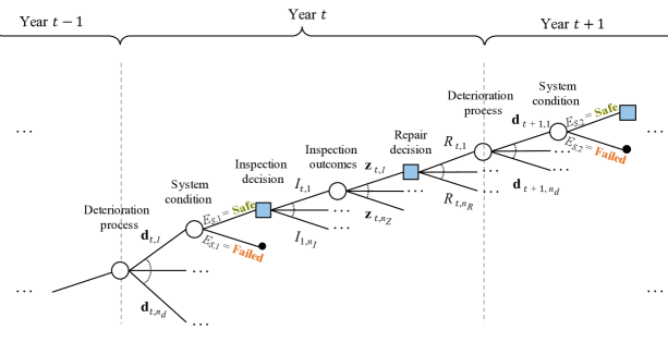
Figure 1: Detail of a decision tree for a deteriorating system which can be inspected and repaired. Random events and outcomes are represented by round nodes, and decisions by square nodes. The deterioration process includes all possible states of damage that the system components can take. Similarly, the inspection outcomes and repair decisions collect all the data and actions for all system components.

Numerous algorithms have been proposed towards the solution of this general optimization problem. The founding algorithms were developed in the 1950s in the field of operations research (OR) to tackle a large variety of problems, from optimizing the location of warehouses in order to minimize transportation costs, to the management of a baseball team (Howard, 1960). Bellman and Howard described solution strategies for fully observable Markovian decision processes (MDPs), based on Bellman’s Dynamic Programming tool (Bellman, 1957a, b; Howard, 1960). Raiffa and Schlaifer (1961) formally included the uncertainty associated with the information acquired during the decision process, paving the way to the study of partially observable MDPs (POMDPs) (Åström, 1965; Kaelbling et al., 1998).

The POMDP approach attempts to provide a universal plan for decision problems where the process is Markovian, and, in theory, accounts for all possible scenarios (Kochenderfer, 2015). (Papadimitriou and Tsitsiklis, 1987) showed that the exact solution of the finite-horizon POMDP cannot be found in polynomial time and is indeed PSPACE-complete. (Bellman, 1957a) coined the term curse of dimensionality and Pineau et al. (2006) added the term curse of history to describe this complexity. Approximate and tractable offline and online solutions for POMDPs using point-based value iteration solvers and belief state approximations are available and have been applied to selected I&M planning problems (Durango and Madanat, 2002; Papakonstantinou and Shinozuka, 2014; Nielsen and Sørensen, 2015; Memarzadeh and Pozzi, 2016; Schöbi and Chatzi, 2016; Papakonstantinou et al., 2018). These approaches perform well where the dimensionality of the problem remains moderate. However, they scale poorly for large multi-component systems, which can easily have a state-space of size $10^{100}$ or larger (Bismut et al., 2017).

An alternative to classical POMDP solvers is a direct policy search (Ng et al., 2000; Rosenstein and Barto, 2001; Powell, 2011), in which one aims at identifying directly and jointly the optimal set of rules for all decisions. This is analogous to the normal form of the decision analysis described by Raiffa and Schlaifer (1961). Sutton et al. (2000) have shown that direct policy search implemented through policy-gradient methods present algorithmic and convergence advantages over value-iteration-based POMDP solvers. Direct policy search does not require Markovian assumptions on the model, nor the explicit computation of the belief states. Direct policy search is also the basis for policy search algorithms using deep neural networks. Popular in the field of motion planning and robotics (e.g. Chebotar et al., 2017), these algorithms have recently been adapted to I&M planning and address the high dimensionality of the problem (Andriotis and Papakonstantinou, 2019).

In the context of I&M planning, the engineering understanding allows the identification of suitable functional forms of the policies. We call these heuristics. For example, a simple heuristic is to perform an inspection campaign whenever the reliability of the structure falls below a threshold. Through such heuristics, the implementation of a direct policy search is straightforward. The optimization is performed over a few heuristic parameters to search the space of policies (Section 2.2.1 expands on this methodology). In the context of optimizing inspections for structural components, it has been found that heuristics lead to solutions that are very close to the optimum POMDP solutions in terms of the resulting expected total life-cycle costs (Nielsen and Sørensen, 2015).

Most RBI planning methodologies are based on such heuristic strategies, mostly in an ad-hoc manner (e.g. Thoft-Christensen and Sørensen, 1987; Lam and Yeh, 1994; Faber et al., 2000; Straub, 2004; Moan, 2005; Nielsen and Sørensen, 2014). These methodologies perform the optimization component-by-component, without considering the interaction among components. Hence it cannot be ensured that the resulting plans are optimal at the system level. In fact, (Luque and Straub, 2019) show that component-based optimization can lead to strongly sub-optimal I&M plans. (Straub, 2004; Straub and Faber, 2005) consider an extension to address system effects in a simplified manner. Other studies have proposed a heuristic-based maintenance planning for series and parallel systems with independent or fully correlated failure modes, but do not account for the effect of inspection results on the components and system reliability (Barone and Frangopol, 2014).

(Luque and Straub, 2019) extend the heuristic approach to a system-level I&M planning, which accounts for the interdependence among components. The methodology relies on the computation of the system reliability by means of a dynamic Bayesian network (DBN) model developed in (Straub, 2009; Luque and Straub, 2016). They evaluate the expected cost of selected system-level I&M plans without performing a formal optimization. Here, we extend the methodology by optimizing the plans by means of the cross entropy method (Rubinstein and Kroese, 2017). The I&M plans are evaluated in terms of expected total life-cycle I&M cost and failure risk. Heuristic parameters are proposed that prescribe inspection times and locations.

A major contribution of this paper is the introduction of adaptive planning, whereby the heuristic I&M plan is modified as new information through inspections and monitoring becomes available. We show that re-optimizing the heuristic parameters once new information is available leads to better I&M plans.

Section 2 summarizes the general methodology for heuristic optimization and introduces the adaptive approach. In Section 3, we first address the computation of the expected total life-cycle cost and then propose the use of the cross-entropy method for solving the optimization problem. In Section 4, we discuss the choice of heuristics for I&M planning in structural systems. Section 5 presents the application of the methodology to a steel structure subjected to fatigue that includes correlation among components. It is followed by results and discussion in Sections 6 and 7.

2 Optimal adaptive heuristic planning

2.1 The generic strategy optimization problem

The premises of the problem are summarized in the following.

1. We assume that a model describing the dynamics of the system (deterioration, loads, structural response), including a prior probabilistic model of uncertain parameters, is available to the analyst. The state of the system is represented by random variables $\bm{\Theta}$, which include the time varying system capacity and the applied loads.

2. We consider a discrete-time model with a fixed finite-horizon $T$, which is typically the anticipated service life of the system. A finite service life is a reasonable assumption since the durability of materials, technological advances, changing user demands and requirements are likely to make the structure obsolete eventually. The service life is in general subject to uncertainty; the effect this could have on the results is not further investigated in this paper. Time is discretized; $i$ indicates the $i^{th}$ time step between times $t_{i-1}$ and $t_{i}$, where $t_{0}=0$ is the beginning of the system’s service life. $n_{T}$ denotes the last time step between times $t_{n_{T}-1}$ and $t_{n_{T}}=T$.

3. A policy $\pi_{i}$ is the set of rules adopted at time step $i$ guiding the decision process based on the information available at that time (Jensen et al., 2007). When considering a deteriorating multi-component system, the policy takes as input all or part of the current knowledge on the state of the system, and gives the answer to the questions ‘Inspect?’ {yes, no}, ‘Where?’ {component $j,\leavevmode\nobreak\ k$, …},‘What to look for?’ {corrosion, fatigue,…} ,‘How?’ {visually, ultrasonic inspection, thickness measurements, …}, ‘Repair?’ {yes, no, how}. The system knowledge includes the history of inspection outcomes, monitoring data, repairs and component failures. A policy is stochastic if it assigns an action following a probability distribution; it is otherwise deterministic. Here we consider deterministic policies, but the general methodology is applicable to either type of policies.

4. A strategy $\mathcal{S}=\{\pi_{1},\pi_{2},...\pi_{n_{T}}\}$ is the set of policies for all time steps. $\mathscr{S}$ is the space of all strategies. A strategy is stationary if its policies are identical for all time steps, i.e. $\pi_{1}=\pi_{2}=...=\pi_{n_{T}}=\pi$.

5. A heuristic parametrizes a strategy. A heuristic strategy is denoted by $\mathcal{S}_{\bm{w}}$ and is governed by heuristic parameters $\bm{w}=\{w_{1},w_{2},...w_{h}\}$.

6. $\bm{Z}=\{\bm{Z}_{1},...,\bm{Z}_{n_{T}}\}$ are random vectors describing inspection and monitoring outcomes collected during the service life of the structure. $\bm{Z}_{1:i}$ denotes the vector of outcomes collected up to time step $i$.

7. $N$ is the number of system components considered for inspection. The components are typically indexed by $k$.

The optimization of the sequential decision process aims to identify the decision strategy $\mathcal{S}^{*}$ that minimizes the expected total life-cycle cost:

$$\mathcal{S}^{*}=\underset{\mathcal{S}\in{\mathscr{S}}}{\arg\min}\leavevmode\nobreak\ \mathbf{E}[C_{\text{tot}}|\mathcal{S}],$$ (1)

where $C_{\text{tot}}$, also written as $C_{\text{tot},1:{n_{T}}}$, is the discounted total life-cycle cost, including inspections, repairs, and possible failures of the system occurring within the time horizon $T$. $\mathbf{E}[C_{\text{tot}}|\mathcal{S}]$ is the expected total life-cycle cost when strategy $\mathcal{S}$ is implemented. Its computation is described in Section 3. The next section summarizes the heuristic approach to solving the optimization problem of Equation 1 and thereafter introduces the adaptive heuristic planning.

2.2 Direct policy search and adaptive search

2.2.1 Direct policy search with heuristic parameters $\bm{w}$

First consider a system with $N$ components that can be inspected, then potentially repaired, at every time step $i$. There are three possible courses of action: either one does nothing, or inspects and based on the inspection result either repairs or does not repair. The total number of possible actions at each time step is $n_{actions}=3^{N}$. All observations from inspection and monitoring during a time step $i$ are summarized in $\bm{Z}_{i}$, which has a discrete outcome space of size $n_{obs}$. In the simplest case, the inspection outcome for each component is either no inspection, or inspection and no detection, or inspection and detection, in which case $n_{obs}=3^{N}$.

A deterministic policy $\pi_{i}$ at time step $i$ chooses an action among the $3^{N}$ options, in function of the observation history, which can take $n_{obs}^{i}$ distinct realizations. Hence, the total number of potential policies at time step $i$ is $3^{N{n_{obs}^{i}}}$. It follows that there are $\prod_{i=1}^{n_{T}}3^{N{n_{obs}^{i}}}={3}^{N\frac{n_{obs}^{n_{T}}-1}{n_{obs}-1}}$ distinct strategies. This illustrates how the space of strategies $\mathscr{S}$ increases exponentially with the number of time steps $n_{T}$ and the number $N$ of system components.

Going through each of the $3^{Nn_{T}}n_{obs}^{\frac{n_{T}^{2}+n_{T}}{2}}$ strategies is clearly impossible. Instead, the solution space $\mathscr{S}$ is reduced by choosing a suitable heuristic, parametrized by $\bm{w}=\{w_{1},w_{2},...w_{h}\}$. A simple (although likely suboptimal) example of a heuristic is: Inspect all components of the structure whenever the reliability estimate is below a threshold, then repair all components at which defects are found. In this case, the only heuristic parameter is the reliability threshold. The strategies $\mathcal{S}_{\bm{w}}$ resulting from such a heuristic form a subspace of $\mathscr{S}$.

The solution $\mathcal{S}^{*}$ to the optimization problem in Equation 1 is therefore approximated by $\mathcal{S}_{\bm{w}_{0}^{*}}$, where

$$\bm{w}_{0}^{*}=\underset{\bm{w}}{\arg\min}\leavevmode\nobreak\ \mathbf{E}\left[C_{\text{tot}}|\mathcal{S}_{\bm{w}}\right].$$ (2)

From this point forward, we use $\mathbf{E}[\cdot|\bm{w}]$ to denote $\mathbf{E}[\cdot|\mathcal{S}_{\bm{w}}]$ for the sake of simplicity in the notation.

Restricting the optimization of Equation 1 to the heuristic space of strategies has two effects: firstly, it reduces the solution space; secondly, the heuristic parameters, such as a reliability threshold, can take continuous values.

One challenge is the selection of the heuristic, so that the strategies explored are close enough to the exact solution of Equation 1. In the context of machine learning, this selection is controlled by hyperparameters that can in turn be optimized, or "tuned". This tuning aspect is not investigated further in the paper.

For I&M problems, the choice of heuristics is often driven by operational constraints, such as the need for regular inspection intervals. The heuristic can also include reliability criteria that need to be fulfilled (Tsang, 1995; Nielsen and Sørensen, 2014). The heuristics are also not required to incorporate information about the system. For instance, a valid strategy is one that prescribes to replace a system every 10 years, regardless of its actual state of deterioration or of any prior collected information. Such systematic plans are typically adopted for non-crucial components of a system (e.g. air filters of an air handling unit); they are rarely based on a quantitative optimization, however. We introduce heuristics for I&M planning in deteriorating structures in Section 4.

2.2.2 Adaptive policy search

Following Equation 2, the optimal heuristic is found initially and kept throughout the system lifetime $T$. However, as new observations $\bm{Z}_{1:i}$ become available, the initially optimal strategy may no longer be optimal. Therefore, we suggest to adapt the strategy during the lifetime of the structure by adding an on-line computation that accounts for the new observations $\bm{Z}_{1:i}$.

Initially, one performs the optimization with the prior model following Equation 2 to obtain the optimal parameters $\bm{w}_{0}^{*}$. To make this explicit, the actions (e.g. inspections and eventual repairs) are performed as dictated by $\bm{w}_{0}^{*}$ until a time step $j_{1}$, typically when new information is available. At $t_{j_{1}}$, the decision maker has the opportunity to improve the strategy.

By updating the prior model with information obtained up to time $t_{j_{1}}$, $\bm{Z}_{1:j_{1}}$, a heuristic strategy optimization is again performed for the rest of the service life of the structure, and a new parameter value $\bm{w}_{1}^{*}$ and its associated strategy are obtained (Equation 3).

$$\bm{w}_{1}^{*}=\underset{\bm{w}}{\arg\min}\leavevmode\nobreak\ \mathbf{E}\left[C_{\text{tot},j_{1}:n_{T}}|\bm{w},\bm{Z}_{1:j_{1}}\right].$$ (3)

$C_{\text{tot},j_{1}:n_{T}}$ is the total cost evaluated from time step $j_{1}$ onwards, as opposed to $C_{\text{tot},1:n_{T}}$, evaluated from time step $1$ onwards. $\mathbf{E}\left[\cdot|{\bm{w},\bm{Z}_{1:j_{1}}}\right]$ is the expectation operator conditional on the observation and repair history up to time step $j_{1}$, applying strategy parameters $\bm{w}$.

It follows from Equation 3 that

$$\mathbf{E}\left[C_{\text{tot},j_{1}:n_{T}}|\bm{w}_{0}^{*},\bm{Z}_{1:j_{1}}\right]\geq\mathbf{E}\left[C_{\text{tot},j_{1}:n_{T}}|\bm{w}_{1}^{*},\bm{Z}_{1:j_{1}}\right].$$ (4)

Our aim is to show that the adaptive planning decreases the expected total life-cycle cost. For this purpose, we decompose the expected total life-cycle cost of strategy $\bm{w}_{0}^{*}$ into

$$\mathbf{E}\left[C_{\text{tot},1:n_{T}}|\bm{w}_{0}^{*}\right]=\mathbf{E}\left[C_{\text{tot},1:j_{1}}|\bm{w}_{0}^{*}\right]+\mathbf{E}_{\bm{Z}_{1:j_{1}}}\left[\mathbf{E}\left[C_{\text{tot},j_{1}:n_{T}}|\bm{w}_{0}^{*},\bm{Z}_{1:j_{1}}\right]\right],$$ (5)

where $C_{\text{tot},1:\tau_{1}}|\bm{w}_{0}^{*}$ is the cost incurred until time $t_{j_{1}}$ following strategy $\mathcal{S}_{\bm{w}_{0}^{*}}$. The expectation $\mathbf{E}_{\bm{Z}_{1:j_{1}}}[\cdot]$ operates on the observation and repair history up to time step $j_{1}$. This operator preserves the inequality in Equation 4, hence by combining Equations 4 and 5, we obtain that

$$\mathbf{E}\left[C_{\text{tot},1:n_{T}}|\bm{w}_{0}^{*}\right]\geq\mathbf{E}\left[C_{\text{tot},1:j_{1}}|\bm{w}_{0}^{*}\right]+\mathbf{E}_{\bm{Z}_{1:j_{1}}}\left[\mathbf{E}\left[C_{\text{tot},j_{1}:n_{T}}|\bm{w}_{1}^{*},\bm{Z}_{1:j_{1}}\right]\right].$$ (6)

The difference between the left and right hand side of Equation 6 quantifies the expected gain by adapting the strategy at time $t_{j_{1}}$. Figure 2 retraces the steps of this strategy improvement.

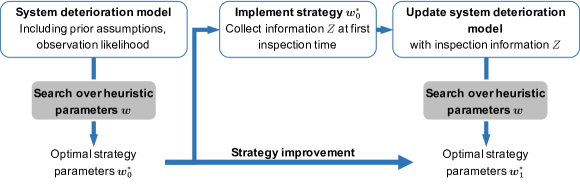
Figure 2: One-step adaptive I&M planning with heuristic search

In the context of production and supply optimization, a similar approach is known as model predictive control (MPC) (Pooya and Pakdaman, 2018). The principle is also adopted to improve reinforcement learning algorithms (Kahn et al., 2017), and is key to the Monte Carlo Tree Search POMCP algorithm presented in (Silver and Veness, 2010).

The strategy adaptation can be repeated every time new information is collected. The array $\bm{W}^{*}$ stores the successively adapted heuristic parameters values:

$$\bm{W}^{*}=\{\bm{w}_{0}^{*},\bm{w}_{1}^{*},\bm{w}_{2}^{*},…,\bm{w}_{n_{ADAPT}}^{*}\},$$ (7)

Algorithm 1 summarizes the adaptive planning method.

input : heuristic, number of times steps $n_{T}$ for time horizon $T$,

adaptation times $\bm{j}=\{j_{1},\dots,j_{n_{ADAPT}}\}$, $prior\_model$

output : $\bm{W}^{*}$

$l\leftarrow 0$;

$model\leftarrow prior\_model$;

repeat

       $\bm{w}^{*}_{l}\leftarrow\underset{\bm{w}}{\arg\min}(\mathbf{E}[C_{\text{tot},j_{l+1}:n_{T}}|\bm{w},model])$ ;

        $\triangleright$ find optimal heuristic parameters, e.g. with Algorithm 2

       $l\leftarrow l+1$;

       if $\text{no system failure before}\leavevmode\nobreak\ t_{j_{l}}$ then

             Perform inspections and repairs following $\bm{w}_{l-1}^{*}$ until $t_{j_{l}}$

            $model\leftarrow update\_model(model,\bm{z_{1:j_{l}}})$;

              $\triangleright$ update deterioration model with $\bm{z}_{1:j_{l}}$

            

       end if

      

until $l>n_{ADAPT}$;

return $\bm{W}^{*}=\{\bm{w}_{0}^{*},...,\bm{w}_{n_{ADAPT}}^{*}\}$

Algorithm 1 Procedure for adaptive I&M planning

The proposed adaptive planning is an on-line optimization at the level of array $\bm{W}^{*}$ and is greedy since the strategy optimization is always performed assuming that it is the last opportunity to optimize the strategy. Multi-step-based improvement greedy techniques have demonstrated to perform much better than a single initial optimization, as shown empirically with a number of algorithms (Silver and Veness, 2010; Pooya and Pakdaman, 2018; Efroni et al., 2018).

3 Stochastic computation and optimization

3.1 Expected total cost of a strategy

3.1.1 Cost breakdown

The heuristic approach requires the computation of the objective function $\mathbf{E}[C_{\text{tot}}|\bm{w}]$ in Equation 2. The influence diagram of Figure 3 shows all costs incurred during the service life of the structure.

The expectation $\mathbf{E}[C_{\text{tot}}|\bm{w}]$ of the total cost of a strategy operates on the state of the system $\bm{\Theta}$, which includes the time varying system capacity and the applied loads, and on the observation outcomes $\bm{Z}\in\Omega_{\bm{Z}}$.

$$\mathbf{E}[C_{\text{tot}}|\bm{w}]=\mathbf{E}_{\bm{\Theta},\bm{Z}}[C_{\text{tot}}|\bm{w}]=\int_{\Omega_{\bm{\Theta}}}\int_{\Omega_{\bm{Z}}}{C_{\text{tot}}(\bm{w},\mathbf{z},\bm{\theta})f_{\bm{\Theta},\bm{Z}|\bm{w}}(\bm{\theta},\mathbf{z}|\bm{w})\mathrm{d}\mathbf{z}\mathrm{d}\bm{\theta}},$$ (8)

where $f_{\bm{\Theta},\bm{Z}|\bm{w}}(\bm{\theta},\mathbf{z}|\bm{w})$ is the joint probability distribution of $\bm{\Theta}$ and $\bm{Z}$ conditional on the strategy parameters $\bm{w}$.

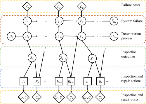
Figure 3: Influence diagram for the decision process. The square nodes indicate the inspection and repair decisions, and the diamond shaped nodes the inspection, repair and failure costs.

This expectation can be approximated with crude Monte Carlo simulation (MCS). However, when the expected costs involve the risk of failure, and if the underlying probability of failure is small, then the Monte Carlo sampling over both $\bm{\Theta}$ and $\bm{Z}$ is computationally expensive because a large number of samples is necessary to achieve an acceptable accuracy. Therefore, following (Luque and Straub, 2019) we propose to first evaluate the expected costs conditional on $\bm{Z}$ (Equation 10), and then perform a MCS over the observation history $\bm{Z}$. To this end, Equation 8 is rewritten as

$$\mathbf{E}[C_{\text{tot}}|\bm{w}]=\int_{\Omega_{\bm{Z}}}{\mathbf{E}_{\bm{\Theta}|\mathbf{z}}[C_{\text{tot}}(\bm{w},\mathbf{z},\bm{\Theta})|\bm{w},\mathbf{z}]f_{\bm{Z}|\bm{w}}(\mathbf{z}|\bm{w})\mathrm{d}\mathbf{z}},$$ (9)

where $f_{\bm{Z}|\bm{w}}(\mathbf{z}|\bm{w})$ is the probability density function of the service life observations $\bm{Z}$ conditional on $\bm{w}$. The corresponding Monte Carlo estimate is detailed in Section 3.1.4.

The total life-cycle cost $C_{\text{tot}}(\bm{w},\bm{Z},\bm{\Theta})$ is the sum of the inspection campaign costs $C_{C}(\bm{w},\bm{Z},\bm{\Theta})$, component inspection costs $C_{I}(\bm{w},\bm{Z},\bm{\Theta})$, repair costs $C_{R}(\bm{w},\bm{Z},\bm{\Theta})$ and failure costs $C_{F}(\bm{w},\bm{Z},\bm{\Theta})$ over the lifetime of the structure. All these costs are present values, i.e., they are discounted to time $0$. Hence the expected total life-cycle cost conditional on the observation outcomes $\bm{Z}$ for given heuristic parameters $\bm{w}$ is

$$\mathbf{E}_{\bm{\Theta}|\bm{Z}}[C_{\text{tot}}|\bm{w},\bm{Z}]=\mathbf{E}_{\bm{\Theta}|\bm{Z}}[C_{I}|\bm{w},\bm{Z}]+\mathbf{E}_{\bm{\Theta}|\bm{Z}}[C_{C}|\bm{w},\bm{Z}]+\mathbf{E}_{\bm{\Theta}|\bm{Z}}[C_{R}|\bm{w},\bm{Z}]+\mathbf{E}_{\bm{\Theta}|\bm{Z}}[C_{F}|\bm{w},\bm{Z}].$$ (10)

The following sections detail how the individual terms in Equation 10 are evaluated.

3.1.2 Computing the conditional risk of failure

Failure is here considered a terminal event. This means that if failure of the system occurs before the end of the service life, no further inspection and repair actions are explicitly considered from that point on. This simplifying assumption does not significantly affect the estimate of the expected total life-cycle cost, due to the high reliability of infrastructure systems (Kübler and Faber, 2004). The fixed cost $c_{F}$ in case of failure includes replacement costs and future life-cycle costs of the new structure. When failure occurs at time $t$, the associated cost expressed as present value is $\gamma(t)\cdot c_{F}$, where $\gamma(t)$ is the discount factor.

The conditional risk of failure over the lifetime of the structure $\mathbf{E}_{\bm{\Theta}|\bm{Z}}[C_{F}|\bm{w},\bm{Z}]$ can be defined in terms of $T_{F}$, the time to failure of the system. $T_{F}$ is a random variable, and is dependent on the implemented strategy $\mathcal{S}_{\bm{w}}$ and the system history $\bm{Z}$. Its probability distribution function (pdf) is denoted by $f_{T_{F}|\bm{w},\bm{Z}}(t)$. It is

$$\mathbf{E}_{\bm{\Theta}|\bm{Z}}[C_{F}|\bm{w},\bm{Z}]=\mathbf{E}_{T_{F}|\bm{Z}}[C_{F}|\bm{w},\bm{Z}]=\int_{0}^{T}{c_{F}\cdot\gamma(t)\cdot f_{T_{F}|\bm{w},\bm{Z}}(t)\mathrm{d}t}.$$ (11)

As time is discretized in $n_{T}$ time steps (years), the integration in Equation 11 is approximated by

$$\mathbf{E}_{\bm{\Theta}|\bm{Z}}[C_{F}|\bm{w},\bm{Z}]\simeq c_{F}\cdot\sum_{i=1}^{n_{T}}{\gamma(t_{i})\cdot\left[F_{T_{F}|\bm{w},\bm{Z}}(t_{i})-F_{T_{F}|\bm{w},\bm{Z}}(t_{i-1})\right]},$$ (12)

where $F_{T_{F}|\bm{w},\bm{Z}}$ is the cumulative distribution function (CDF) of the conditional $T_{F}$. In particular, $[F_{T_{F}|\bm{w},\bm{Z}}(t_{i})-F_{T_{F}|\bm{w},\bm{Z}}(t_{i-1})]$ is the annual probability of failure for year $i$. We compute this annual probability of failure conditional on the observation outcomes with the DBN model described in Section 3.2.

3.1.3 Computing the conditional expected inspection and repair costs

Since failure is a terminal event, the evaluations of expectations $\mathbf{E}_{\bm{\Theta}|\bm{Z}}[C_{I}|\bm{w},\bm{Z}]$, $\mathbf{E}_{\bm{\Theta}|\bm{Z}}[C_{C}|\bm{w},\bm{Z}]$ and $\mathbf{E}_{\bm{\Theta}|\bm{Z}}[C_{R}|\bm{w},\bm{Z}]$ consider that an observation or repair action at a time $t_{i}$ can occur only if the system has survived until that time. For instance, the conditional expected life-cycle inspection campaign costs are calculated as

$$\mathbf{E}_{\bm{\Theta}|\bm{Z}}[C_{I}|\bm{w},\bm{Z}]=\sum_{i=1}^{n_{T}}{\gamma(t_{i})\cdot c_{I}(t_{i},\bm{w},\bm{Z})\cdot\left[1-F_{T_{F}|\bm{w},\bm{Z}}(t_{i})\right]},$$ (13)

where $c_{I}(t_{i},\bm{w},\bm{Z})$ is the inspection campaign cost incurred at time $t_{i}$ as prescribed by strategy $\bm{w}$ and inspection history $\bm{Z}$, and $1-F_{T_{F}|\bm{w},\bm{Z}}(t_{i})$ is the probability of survival of the system up to time $t_{i}$.

Similarly, the conditional expected life-cycle component inspection cost and life-cycle repair cost are evaluated as

$$\mathbf{E}_{\bm{\Theta}|\bm{Z}}[C_{C}|\bm{w},\bm{Z}]=\sum_{i=1}^{n_{T}}{\gamma(t_{i})\cdot c_{C}(t_{i},\bm{w},\bm{Z})\cdot\left[1-F_{T_{F}|\bm{w},\bm{Z}}(t_{i})\right]},$$ (14)

$$\mathbf{E}_{\bm{\Theta}|\bm{Z}}[C_{R}|\bm{w},\bm{Z}]=\sum_{i=1}^{n_{T}}{\gamma(t_{i})\cdot c_{R}(t_{i},\bm{w},\bm{Z})\cdot\left[1-F_{T_{F}|\bm{w},\bm{Z}}(t_{i})\right]},$$ (15)

3.1.4 Monte Carlo simulation over inspection history $\bm{Z}$

In Equation 8, the conditional expectation $\mathbf{E}_{\bm{\Theta}|\bm{Z}}[C_{\text{tot}}|\bm{w},\bm{Z}]$ must be integrated over all possible outcomes $\bm{Z}$. The integral over $\bm{Z}$ cannot be easily computed analytically, as the probability density of all possible inspection outcomes $f_{\bm{Z}|\bm{w}}(\mathbf{z})$ is not readily available.

However, sampling from this distribution is possible, by first generating deterioration histories from the model, and then generating inspection outcomes $\mathbf{z}^{(q)}$ conditional on the deterioration and the adopted strategy. In the case of the adaptive optimization presented in Section 2.2.2, the deterioration histories have to be generated conditional on the past inspection outcomes. It is then necessary to resort to a Bayesian sampling method. Here we employ the BUS methodology with SuS (Straub and Papaioannou, 2015). Equation 8 can then be approximated by MCS:

$$\mathbf{E}[C_{\text{tot}}|\bm{w}]\simeq\frac{1}{n_{MC}}\sum_{q=1}^{n_{MC}}\mathbf{E}_{\bm{\Theta}|\mathbf{z}^{(q)}}[C_{\text{tot}}|\bm{w},\mathbf{z}^{(q)}].$$ (16)

Notably, this MCS over $\bm{Z}$, conditional on a strategy $\mathcal{S}_{\bm{w}}$, does not need to generate samples that lead to the failure of the system. The probability of failure is included in the risk of failure $\mathbf{E}_{\bm{\Theta}|\mathbf{z}^{(q)}}[C_{F}|\bm{w},\mathbf{z}^{(q)}]$, which is calculated directly conditional on each sample history $\mathbf{z}^{(q)}$ as per Equation 12. B discusses the accuracy of MCS to evaluate the risk of failure. In numerical investigations, it was found that a quite small number of samples is sufficient to obtain a good approximation of the expected total life-cycle cost, in the order of 200 samples.

One can break down the expected costs into annual values. Figure 4(a) shows this breakdown for a selected strategy from the numerical application presented in Section 5, evaluated with $n_{MC}=200$ samples. Figure 4(b) shows the effect of the discount factor $\gamma(t)$ on the distribution of the costs for the same strategy.

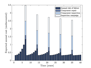
(a) undiscounted

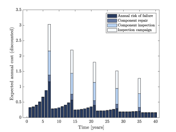
(b) discounted

Figure 4: Expected annual costs for strategy $\mathcal{S}_{\bm{w}_{0}^{*}}$, evaluated with 200 samples, undiscounted (a), and discounted (b) with annually compounded discount rate $r=0.02$.

3.2 Conditional reliability of a deteriorating multi-component system

The computation of the expected cost of failure $\mathbf{E}_{\bm{\Theta}|\bm{Z}}[C_{F}|\bm{w},\bm{Z}]$ in Equation 12 requires the evaluation of the CDF $F_{T_{F}|\bm{w},\bm{Z}}$ of the time to system failure, $T_{F}$.

In this paper, failure of the system originates from the deterioration processes, which gradually decrease the system capacity. Deterioration has been modelled by stochastic processes (e.g Lin and Yang, 1985; van Noortwijk, 2009; Shafiee et al., 2015), or by physics-based equations with uncertain model parameters (e.g. Madsen et al., 1987).

The evaluation of expected costs of I&M strategies requires many reliability evaluations conditional on inspection results. This calls for methods that can efficiently compute conditional reliabilities and can handle a large number of random variables.

Such efficient computation can be available when using Markov chain models for representing deterioration. In general, deterioration processes are non-Markovian, in that the damaged state is not independent of the past states. However, non-Markovian deterioration processes can be transformed into Markovian processes by state-space augmentation (Straub, 2009). The Markov chain model has been extensively used in I&M research (e.g. Rosenfield, 1976; Rausand and Høyland, 2004; Bocchini et al., 2013; Faddoul et al., 2013; Zhu et al., 2013).

In the majority of real multi-component structural systems, components’ deterioration processes are correlated due to common manufacturing conditions and similar environmental and load conditions. To represent deteriorating multi-component systems with interdependent components, standard Markov chain models are not suitable. Instead, we employ the hierarchical dynamic Bayesian network (DBN) of Figure 5. This is a variant of the DBN model of (Luque and Straub, 2019).

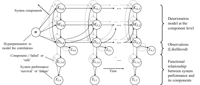
Figure 5: DBN for a deteriorating multi-component system. The correlations between components are explicitly modeled through hyperparameters $\bm{\alpha}$. The state of the system is described by nodes $E_{S,i}$, conditionally on the state of each component, $E_{C,N,i}$, through a function relating components to system state, e.g. a pushover analysis. Evidence is set on the observation nodes $Z_{k,i}$ when the chosen I&M strategy prescribes it.

In the model of Figure 5, each component is represented by its own DBN. These are connected by the hyperparameters $\bm{\alpha}$, which represent the dependence among component deterioration, and the common system performance nodes, which here take states ‘survival’ or ‘failure’. Observations of deterioration state $D_{k,i}$ of component $0\leq k\leq N$ from inspections or monitoring are represented by $Z_{k,i}$. The states of all random variables are discretized according to (Straub, 2009). Exact inference algorithms are implemented to evaluate the probability distributions of all random variables conditional on the observations. For details on the modeling and computation in this hierarchical DBN model we refer to Luque and Straub (2016).

To improve the computational performance, the nodes $E_{S,i}$ represent the state of the system at time step $i$, if the system does not have to opportunity to fail earlier. This is highlighted by the fact that no arrows link temporally the nodes $E_{S,i}$. We call the event $\{E_{S,i}=\text{`failure'}\}=F_{i}^{*}$, the interval failure event (Straub et al., 2020).

The evaluation of this DBN results in the conditional probability of $F_{i}^{*}$ given the observation from all components. By introducing the event $F_{i}$ as ‘failure of the system up to time $t_{i}$’, we note that $F_{i}=F_{1}^{*}\cup F_{2}^{*}\cup…\cup F_{i}^{*}$. One can express the CDF $F_{T_{F}|\bm{w},\bm{Z}}(t_{i})$, as

$$F_{T_{F}|\bm{w},\bm{Z}}(t_{i})=\text{Pr}(F_{i}|\bm{w},\bm{Z})=\text{Pr}(F_{1}^{*}\cup F_{2}^{*}\cup…\cup F_{i}^{*}|\bm{w},\bm{Z}).$$ (17)

In some systems, the events $F_{i}^{*}$ can be assumed to be independent for different $i$. In this case, $\text{Pr}(F_{i}|\bm{w},\bm{Z})$ can be evaluated as

$$\text{Pr}(F_{i}|\bm{w},\bm{Z})=1-\prod_{1\leq j\leq i}{1-\text{Pr}(F_{j}^{*}|\bm{w},\bm{Z})}$$ (18)

The annual probability of system failure for time step $i$ conditional on the observations $\bm{Z}$ is

$$\text{Pr}(F_{i}|\bm{w},\bm{Z})-\text{Pr}(F_{i-1}|\bm{w},\bm{Z}).$$ (19)

The DBN model is flexible with respect to the choice of a-priori probability distributions and transition probabilities. The DBN framework, however, has limitations with respect to the number of parameters in the deterioration models, but work-around strategies exist as discussed in Luque and Straub (2016).

The interval probabilities of failure $(\text{Pr}(F_{i}^{*}|\bm{w},\bm{Z}))_{0\leq i\leq T}$ are computed with Bayesian inference in the DBN, involving Bayesian filtering, prediction and smoothing algorithms (Askar and Derin, 1981, 1983; Straub, 2009; Särkkä, 2013; Luque and Straub, 2016). The computational cost of this algorithm increases only linearly with the number of components, which makes it suitable for large systems (Luque and Straub, 2016). The cumulative probability of failure $\text{Pr}(F_{i}|\bm{w},\bm{Z})$ and the annual probability of failure are then evaluated with Equations 18 and 19. This implies an approximation, which has shown to be appropriate for the reliability problem investigated in Section 5 (Straub et al., 2020).

It should be noted that alternative methods exist for computing $\text{Pr}(F_{i}|\bm{w},\bm{Z})$. For example, Schneider et al. (2017) applied BUS with SUS for the same structural system as considered in Section 5.

3.3 Stochastic optimization method

Equation 16 provides a noisy approximation of the expected total life-cycle cost for given heuristic parameters defining a strategy. Stochastic optimization methods are well suited to handle noisy objective functions of the form of Equation 16 (Spall, 2012; Hill, 2013). Here, we consider the cross entropy (CE) method (De Boer et al., 2005) combined with a Gaussian process regression (GPR) (Rasmussen, 2004) to approximate the solution of Equation 2 and to find the heuristic parameters values that minimize the exact expected total life-cycle cost.

Algorithm 2 summarizes the steps of the CE method, inspired by (Kochenderfer, 2015). It generates $n_{CE}$ samples $\bm{w}^{(m)}$ of heuristic parameters from a distribution with parameters $\bm{\lambda}^{*}$. For each sample $\bm{w}^{(m)}$, $n_{MC}$ observation and monitoring histories are generated and the expected total life-cycle cost is calculated through Equation 16. The samples $\bm{w}^{(m)}$ are then ranked in ascending order of their estimated expected life-cycle cost. The $n_{E}$ best-ranked $\bm{w}^{(m)}$, also called elite samples, are used to update the CE sampling distribution parameter $\bm{\lambda}^{*}$ by cross entropy minimization. This step is repeated until a convergence criterion has been met, or until a sufficient number $n_{max}$ of strategies have been explored. The convergence speed of the CE method can be optimized by choosing $n_{MC}$ adequately. In particular, the CE method can work with a single sample evaluation in Equation 16, i.e. $n_{MC}=1$, and still converge towards the heuristic parameter values that minimize the exact expected total life-cycle cost (Rubinstein and Kroese, 2004). In addition to the CE method, GPR is applied to all the estimated expected costs calculated during the CE loop. The surrogate function thus obtained is used to approximate $\mathbf{E}[C_{\text{tot}}|\mathcal{S}_{\bm{w}}]$ in Equation 2, and the optimal heuristic parameter values $\bm{w}^{*}$ are obtained by minimizing this surrogate function.

Coupling the CE method with GPR presents the advantage that the surrogate mean and standard error of the mean can be extracted for any point in the heuristic parameter space. This can be used to evaluate the sensitivity of the expected total life-cycle cost to the heuristic parameters. Furthermore, due to the CE sampling method, the standard error of the mean decreases towards the surrogate minimum. This methodology can handle both continuous or discrete heuristic parameters, as illustrated in Section 5.

in : CE sampling distribution $P(\cdot|\bm{\lambda}^{*})$, initial sampling distribution parameter $\bm{\lambda}^{*}$, number of CE samples $n_{CE}$, number of elite samples $n_{E}$, number of observation history samples $n_{MC}$, maximum number of objective function evaluations $n_{max}$.

out : optimal heuristic parameters $\bm{w^{*}}$, minimum total life-cycle cost $C^{*}$, surrogate cost function $f$

$l\leftarrow 0$;

while $l\cdot n_{CE}<n_{max}$ do

       for $m\leftarrow 1$ to $n_{CE}$ do

             $\bm{w}^{(m)}\sim P(\cdot|\bm{\lambda}^{*})$;

              $\triangleright$ generate random heuristic parameter values

             $cost\leftarrow 0$;

             for $q\leftarrow 1$ to $n_{MC}$ do

                   generate an inspection and repair history $\mathbf{z}^{(q)}$ following strategy $\mathcal{S}_{\bm{w}^{(m)}}$;

                   $cost\leftarrow cost+\mathbf{E}_{\bm{\Theta}|\mathbf{z}_{1:n_{T}}^{(q)}}[C_{\text{tot}}|\bm{w}^{(m)},\mathbf{z}^{(q)}]$;

                    $\triangleright$ Eq. 10 to 15

                  

             end for

            $q_{m}\leftarrow cost/n_{MC}$;

              $\triangleright$ expected total life-cycle cost (Eq. 16)

            

       end for

      Store $\bm{w}^{(m)}$, $q_{m}$;

       $\widehat{\bm{w}}^{(1)},..\widehat{\bm{w}}^{(n_{CE})}\leftarrow$Sort $(\bm{w}^{(1)},..\bm{w}^{(n_{CE})})$ in increasing order of $q_{m}$;

       $\bm{\lambda}^{*}\leftarrow\arg\max_{\bm{\lambda}}\sum_{m=1}^{n_{E}}{\log P(\widehat{\bm{w}}^{(m)}|\bm{\lambda})}$;

        $\triangleright$ update $\bm{\lambda}^{*}$ with the elite samples

       $l\leftarrow l+1$;

      

end while

$h\leftarrow GPR(\bm{w}^{(m)},q_{m})$;

  $\triangleright$ build the surrogate function

$\bm{w}^{*}\leftarrow\arg\min h$;

$C^{*}\leftarrow\min h$;

return $\bm{w}^{*},\leavevmode\nobreak\ C^{*},\leavevmode\nobreak\ h$

Algorithm 2 Pseudo-code for the stochastic optimization

3.4 Summary

The methodology is summarized in Figure 6. It is applicable to any deteriorating system with multiple components. The methods for the optimization or for the evaluation of the expected cost of a strategy can be chosen freely, as they will not affect the underlying principles of the methodology. For instance, the CE method can be upgraded to include optimal computing budget allocation (OCBA) (He et al., 2010; Chen and Lee, 2011), which identifies the strategies for which $n_{MC}$ should be increased, to increase the confidence in the selection of the elite parameters. The computational effort is thereby optimized, as is the efficiency of the chosen optimization method.

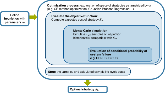
Figure 6: Steps of optimal heuristic planning.

4 Heuristics for I&M planning in structural systems

The proposed approach requires the definition of appropriate heuristics. The heuristic should be sufficiently flexible to ensure that a sufficiently high number of strategies can be explored and that it can define a near-optimal strategy.

As an example, an overly simplistic heuristic is to never inspect and repair systematically at fixed time intervals $\Delta T$. Finding the solution of Equation 2 is then equivalent to an optimization over one heuristic parameter $\bm{w}={\Delta T\in{\{1,..,T\}}}$. It is very likely that a heuristic strategy, which conditions the repair decision on observation outcomes, has a lower expected total life-cycle cost.

4.1 Choosing I&M heuristics

For I&M planning of a multi-component deteriorating system, the possible decisions must answer the elementary questions of ‘when’, ‘where’, ‘what’ and ‘how’ to inspect, and ‘when’, ‘where’, ‘what’ and ‘how’ to repair.

The questions ‘what’ and ‘how’ to inspect and repair are dependent on the deterioration mechanism and are in general determined by expert knowledge of the system, and the availability of repair and inspection techniques. They are not within the scope of this study and are not further discussed.

The questions ‘when’ and ‘where’ to repair can be answered in different ways; in corrective maintenance, repair or replacement occurs upon failure of the system; in systematic preventive maintenance, repair or replacement occurs at times fixed in advance, irrespective of any observation on the state of the system (Barlow and Hunter, 1960; Nielsen and Sørensen, 2010b). The heuristic strategies investigated in this paper are relevant for a condition-based preventive maintenance, where repair actions are decided based on the current condition of the system using inspection and monitoring data. In this approach, a component repair is triggered by an inspection result. With some generality, this repair decision can be parametrized by a threshold $D_{rep}$: Whenever the identified defect exceeds $D_{rep}$, a repair is triggered.

The inspection-related questions are more complex to parametrize and are discussed in the following paragraphs. They are treated sequentially, choosing first ‘when’ and then ‘where’ to inspect.

4.2 ‘When’ to inspect

An inspection can be planned to take place at specific times during the service life of the structure. It can also be triggered by exceeding a threshold $p_{th}$, for instance on the failure rate. This rate can usually be approximated by the annual probability of failure due to the high reliability of the structure. When a monitoring system is in place, an inspection might be triggered by the exceedance of a monitoring data threshold.

A number of scientific studies have focused on I&M planning for a single component, answering the question ‘when’ to inspect (e.g. Thoft-Christensen and Sørensen, 1987; Grall et al., 2002; Straub and Faber, 2006; Nielsen and Sørensen, 2010b). By prescribing regular inspection times, or triggering inspections with a fixed threshold on the probability of failure of the component (Faber et al., 2000), these single-parameter heuristics have proven to yield a strategy that performs similarly in terms of cost and prescribed times of inspection as an optimal strategy found through POMDP or LIMID methods (Nielsen and Sørensen, 2010a; Luque and Straub, 2013).

The choice of a heuristic parameter prescribing an inspection campaign might be based on operational constraints, for instance inspections might have to be planned at regular time intervals $\Delta T$. In other instances, they may arise from established practices.

4.3 ‘Where’ to inspect: component prioritization and value of information

This question is specific to multi-component systems, where inspecting the entire system at every inspection campaign is suboptimal or not even feasible. Rather, one would typically inspect only a subset of all components during an inspection campaign. In order to identify the best components to inspect, we propose a heuristic prioritization rule described by two parameters.

The first heuristic parameter is the number of components $n_{I}$ to inspect at each inspection campaign. A second heuristic parameter $\eta$ is introduced to prioritize the components for inspection at each campaign, as described in the following.

Because of the correlation among the component deterioration, inspecting one component can provide information about the condition of other components. The value of this information can in theory be quantified, as demonstrated in (Straub and Faber, 2005). It seems reasonable to perform the component inspections with the highest value of information (VoI). However, the calculation of the VoI is computationally challenging for multi-component systems.

We introduce instead a Prioritization Index, $PI_{k}$, to serve as a proxy for the VoI and prioritize the components for inspection. This index is calculated for each component $k$ whenever an inspection campaign is launched, based on the information $\bm{Z}_{1:{i-1}}$ collected up to the last inspection time.

The $PI_{k}$ considers two fundamental contributions to the VoI: (a) the reduction of the uncertainty on the condition of the inspected component and the corresponding effect on the system reliability; and (b) the reduction of the uncertainty on the condition of other components, through the components’ interdependence.

These reductions are related to two quantities. The first is the probability of failure of component $k$, $\text{Pr}(F_{c_{k}}|\bm{Z}_{1:{i-1}})$, conditional on all components’ inspection outcomes up to that point. RBI planning revealed in particular that inspecting components with a higher probability of failure provides more information on the deterioration of other components than inspecting components with a lower probability of failure (Straub and Faber, 2005).

The second quantity is the Single Element Importance measure for component $k$ ($SEI_{k}$), defined as the difference between the probability of failure of the intact system and the probability of failure of the system when only component $k$ has failed (Straub and Der Kiureghian, 2011):

$$SEI_{k}=\text{Pr}(F_{s}|\overline{F_{c_{1}}},...,\overline{F_{c_{k-1}}},F_{c_{k}},\overline{F_{c_{k+1}}},...,\overline{F_{c_{N}}})-\text{Pr}(F_{s}|\overline{F_{c_{1}}},...,\overline{F_{c_{N}}})$$ (20)

The VoI of inspection component $k$ is linked to the reduction of the probability of system failure. This probability can be expressed approximately as a linear function of $SEI_{k}$ and $\text{Pr}(F_{c_{k}}|\bm{Z}_{1:{i-1}})$ (Bismut et al., 2017), as detailed in C. Hence, the VoI increases with increasing $(SEI_{k})$ and increasing $\text{Pr}(F_{c_{k}}|\bm{Z}_{1:{i-1}})$.

With an adjustable exponent $\eta$ that serves as a heuristic parameter, the Prioritization Index $PI_{k}$ combines the two effects described above,

$$PI_{k}=(SEI_{k})^{\eta}\cdot\text{Pr}(F_{c_{k}}|\bm{Z}_{1:{i-1}}),\text{ with }\eta\geq 0.$$ (21)

Other factors should be considered for the prioritization, such as the effect of varying component correlations, inspection quality, and cost of inspection. For instance, an underwater part of an offshore structure is more difficult and costly to inspect with the same accuracy as a part of the superstructure. Here, we limit the study to equi-correlated components, with equal inspection quality and cost. Additional factors with corresponding exponents (i.e. additional heuristic parameters) could however be introduced into Equation 21.

5 Numerical application: structural frame subject to fatigue

5.1 Structural model

There are no standard procedures for I&M planning of structures subject to fatigue deterioration. Time-based maintenance is in general not appropriate for this type of deterioration (de Jonge et al., 2017). Condition-based maintenance is typically implemented by fixing an inspection interval between inspection campaigns, and inspecting all or selected components, following unknown heuristics.

We apply the described methodology to the I&M planning of a steel structure representing a jacket support structure of an offshore wind turbine, which is typically subject to fatigue deterioration. We adopt the Zayas frame model (Zayas, 1980), often used for benchmark studies (e.g. Chen and Sohal, 1988; Luque and Straub, 2016; Schneider et al., 2017; Schneider, 2019). This steel frame is composed of two vertical legs, braced by 13 tubular members; 22 fatigue hotspots located at the welds are identified as per Figure 7 and constitute the model components. The states of deterioration of the components are correlated (see Section 5.2). The frame is loaded laterally with a time-varying load, $S_{max,i}$, which represents the maximum load occurring within one time step, or year. We assume that the maximum annual loads are independently distributed, following a lognormal distribution, with mean $50$kN and coefficient of variation $0.53$. Failure is determined by the system components deterioration states and the response of the damage structure to the applied load. The pushover analysis for the frame is from Schneider et al. (2017). The ultimate resistance of the undamaged frame is $282$kN.

Figure 7: Zayas frame. The red dots indicate the locations of 22 fatigue hotspots. The frame is loaded laterally with yearly amplitude $S_{max,i}$. After Schneider et al. (2017)

5.2 Deterioration model

For each component $k$, $D_{k,i}$ indicates the crack depth at time $t_{i}$. The transition from $D_{k,i}$ to $D_{k,i+1}$ is obtained from Equation 22, which models the fatigue crack growth by Paris’ law,

$$\frac{dD}{dt}=C[\Delta S_{e}^{M}\pi^{\frac{M}{2}}]\cdot D(t)^{\frac{M}{2}},$$ (22)

where $C$ and $M$ are empirical material parameters. They are correlated with a correlation coefficient close to $-1$, hence $C$ is here expressed as a linear function of $M$ (Straub, 2004). The initial crack depth is noted $D_{k,0}$ and failure of a component is defined as the fatigue crack size exceeding a critical depth $d_{cr}$.

The fatigue stress range $\Delta S$ is described by a Weibull distribution with scale and shape parameters $K$ and $\lambda$. The distribution of the equivalent fatigue stress range $\Delta S_{e}=(\mathbf{E}[\Delta S^{M}])^{\frac{1}{M}}$ is defined by Equation 23 (Straub, 2004), as

$$\Delta S_{e}=K\cdot\Gamma\left(1+\frac{M}{\lambda}\right)^{\frac{1}{M}}.$$ (23)

$K$ and $M$ are unknown parameters and are assumed constant during the deterioration process. In order to preserve the Markovian assumption, the random variables $K_{k,0\leq i\leq n_{T}}$ and $M_{k,0\leq i\leq n_{T}}$ are introduced in the Bayesian network, such that $K_{k,i+1}=K_{k,i}=K_{k}$ and $M_{k,i+1}=M_{k,i}=M_{k}$. The corresponding DBN is shown in Figure 5.

The distribution of $K_{k}$ for each component $k$ is lognormal, and the mean values are calibrated to a chosen fatigue design factor (FDF). The FDFs represent the ratio between the fatigue life of a component and the service life of the structure. The calibration procedure is explained in A.2. Table 2 lists the components, their FDFs, and the corresponding means of $K_{k}$.

Additionally, the initial crack depths of all components $D_{k,0}$ are equi-correlated with factor $\rho_{D_{0}}$, as are the stress and material parameters, $K_{k}$ and $M_{k}$ with factors $\rho_{K}$ and $\rho_{M}$ respectively. The correlation is reflected in the computation of the probability tables conditional on the hyperparameters $\bm{\alpha}$ of the DBN, following the procedure of (Luque and Straub, 2016).

The model parameters and correlations are summarized in A.1.

5.3 Inspection and repair model

The observation outcome ${Z}_{k,i}$ is a random variable defined conditionally on $D_{t}$. ${Z}_{k,i}$ can take the value {$Z_{k,i}=0$}, indicating {‘no crack detected’}, or values larger than $0$, reflecting a measured crack size. Here, the probability of detection (PoD) $\text{Pr}(Z_{k,i}>0|D_{t}=d)$ is:

$$PoD(d)=1-\text{exp}\left(-\frac{d}{\xi}\right)$$ (24)

In case of detection, the measurement ${Z}_{k,i}$ is normally distributed with mean $D_{k,i}$ and standard error $\sigma_{\epsilon}$. The corresponding hybrid distribution is defined in Equation 25, where $\varphi(.)$ is the standard normal probability density function, and $\Phi(.)$ is the standard normal cumulative distribution function:

$$\begin{cases}\text{Pr}(Z_{k,i}=0|D_{k,i}=d)=1-PoD(d)\\ f_{Z_{k,i}|D_{k,i}=d}(Z_{k,i}=z)=PoD(d)\cdot\frac{1}{1-\Phi\left(\frac{-d}{\sigma_{\epsilon}}\right)}\cdot\varphi\left(\frac{z-d}{\sigma_{\epsilon}}\right)&\text{if }z>0.\end{cases}$$ (25)

If the damage exceeds a threshold $D_{rep}$, the component is repaired immediately and completely. This corresponds to restoring it to its initial state, i.e. the probability distribution of the damage after a repair is the one of $D_{k,0}$. The repaired state is assumed to be uncorrelated with the initial state.

Following from DBN model structure described in Section 3.2 and in Figure 5, the inspection outcome of one component affects the posterior distribution of the crack size of all other components, whether or not the inspected component is repaired.

5.4 Costs of I&M actions

I&M actions incur mobilization costs, repair costs, costs for material supply, workmanship, inspection techniques, and sometimes downtime. Here, all components are attributed the same cost of inspection and repair, which are constant over time. This choice simplifies the problem specification; alternative cost models do not affect the computation efforts or the accuracy of the method.

The following costs are considered:

• $c_{C}$: cost of launching an inspection campaign. It includes the cost of transporting inspection operators to site, and potentially the cost of impairing the operation of the system.

• $c_{I}$: cost of inspection per component. It accounts for the time spent to inspect one component during an inspection campaign.

• $c_{R}$: cost of repairing one component. It also includes the associated downtime.

• $c_{F}$: cost incurred if the structure fails, including full replacement costs and life-cycle costs of the new structure.

All costs are discounted to their present value by the discount factor $\gamma(t)=\frac{1}{(1+r)^{t}}$, where $r$ is the annually compounded discount rate. The parameters of the cost function and discount factor are provided in Table 1.

Table 1: Cost parameters

Parameter	$c_{C}$	$c_{I}$	$c_{R}$	$c_{F}$	$r$
Value	$1$	$0.1$	$0.3$	$3\cdot 10^{3}$	$0.02$

5.5 Heuristic parameter choice

The investigated heuristic includes the following parameters $\bm{w}=\{\Delta T,p_{th},n_{I},\eta\}$:

1. Inspection campaigns are carried out at fixed inspection intervals $\Delta T\in\{1,2,…40\}$ [years].

2. Additionally, when the annual probability of failure of the system exceeds the probability threshold $p_{th}\in[0,1]$, an inspection campaign is carried out.

3. The number of hotspots to be inspected at every inspection campaign is $n_{I}\in\{1,2,…,22\}$.

4. The hotspots are prioritized for inspection following Section 4.3 with parameter $\eta\geq 0$.

The repair threshold $D_{rep}\geq 0$ can also be included as a heuristic parameter. For the purpose of this study, a component is repaired if the deterioration exceeds a threshold value $D_{rep}=0$ at the inspection. This implies that every identified defect is repaired. The results documented in Section 6 show that the expected repair costs are low even with this choice, which indicates that optimizing $D_{rep}$ would not significantly affect the expected life-cycle cost.

5.6 Optimization set up and computation

The CE sampling algorithm is run with MATLAB on a 2.6GHz computer with 24 quad-core processors. The algorithm is optimized for the computation of the conditional probability of system failure. One history life-cycle cost is computed in about 20 CPU minutes, but these computations can be run in parallel.

For the CE optimization method of Algorithm 2, lognormal sampling distributions are employed for the heuristic parameters $p_{th}$ and $\eta$. For the discrete parameters $\Delta T$ and $n_{I}$, a truncated normal distribution is selected, so that the sampled values are within the acceptable bounds; the sampled values are then rounded to the nearest integer. In this numerical application, all sampling distributions are kept uncorrelated and the heuristic parameters are optimized one after the other in a recursive manner. This was mainly for ease of graphical representation of the results. Correlating the distributions might lead to more efficient sampling during the optimization and faster convergence towards the optimal parameter values.

We fix $n_{MC}=1$. About 1600 samples of total life-cycle costs for different strategies are drawn as per Equation 10. To obtain a surrogate of the total life-cycle costs, a GPR is performed on the logarithm of the sample costs. This guarantees that the surrogate function stays positive in the original space. The GPR is implemented with the MATLAB2018 function fitrgp.m and a squared-exponential kernel. The minimum of this surrogate cost function is calculated with the MATLAB2018 function surrogateopt.m.

GPR can also be performed on all four cost components separately: inspection campaign, component inspection, repair and failure risk. However, it was found that the total cost predictions obtained by summing up the four resulting Gaussian processes are not as stable as the predictions obtained by the GPR on the total life-cycle cost, and are therefore not used to find the optimal heuristic parameter values. Figure 9 compares the prediction of the expected total life-cycle cost with the two methods, for selected strategies.

We consider one adaptation of the I&M plan after the first inspection campaign. For the adaptation, the deterioration model is updated with the inspection outcomes at the time prescribed by the initial strategy. Then, 1600 deterioration histories are simulated from the posterior distributions, using BUS SUS (Straub and Papaioannou, 2015). Based on these samples, total life-cycle costs are calculated for different strategies, and the strategy optimization is performed as outlined in Section 2.2.2.

6 Results

6.1 Conditional annual risk computed with DBN

Figure 8(a) depicts an example of the evolution of the computed probabilities for a sample observation history, following the strategy described by heuristic parameters $\{\Delta T=10,\leavevmode\nobreak\ p_{th}=1\cdot 10^{-2},\leavevmode\nobreak\ n_{I}=4,\leavevmode\nobreak\ \eta=1\}$. The corresponding probability of failure of a selected hotspot is plotted in Figure 8(b). It should be noted that the discretization scheme influences the accuracy of these computations, notably when performing Bayesian smoothing. The associated error is investigated in (Zhu and Collette, 2015) and is mainly due to the rough discretization in the failure domain of the component. However, we have found that it does not significantly impact the evaluation of $\text{Pr}(F_{i}^{*}|\bm{w},\bm{Z})$.

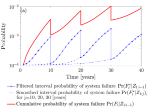
(a)  

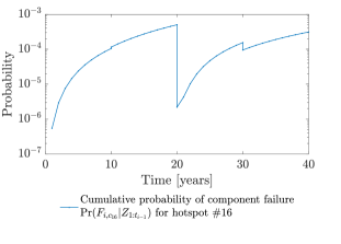
(b)  

Figure 8: (a) Evolution of the interval probability and cumulative probability of system failure for a sample observation history following strategy $\mathcal{S}_{\bm{w}}$, with ${\bm{w}}=\{\Delta T=10,\leavevmode\nobreak\ p_{th}=1\cdot 10^{-2},\leavevmode\nobreak\ n_{I}=4,\leavevmode\nobreak\ \eta=1\}$. The discontinuities indicate that an inspection is performed and the reliability is updated. The dotted blue lines represent the smoothed probabilities $\text{Pr}(F_{j}^{*}|\bm{Z}_{1:i})$, for $j\leq i$, updated with the current system information; (b) corresponding evolution of the probability of failure for hotspot $\sharp 16$. The discontinuities at years {10, 30} are due to inspections on other components in the system. Hotspot $\sharp 16$ is inspected at year 20, and is never repaired in this simulation.

6.2 Optimal heuristic strategy at time $t=0$

First, we investigate how the expected cost varies in function of the different heuristic parameters. Figure 9 shows the total life-cycle cost in function of $n_{I}$ and $\Delta T$ for sample strategies from the CE method. The GPR surrogate estimate is also shown.

As expected, the total life-cycle risk of failure decreases with increasing number $n_{I}$ of hotspots inspected at every inspection campaign. Similarly, strategies with small inspection intervals $\Delta T$ are costly because of the frequency of the inspections; in contrast, strategies with large $\Delta T$ suffer from a larger uncertainty and thus an increased risk of failure. Samples drawn in a similar way for varying $p_{th}$ and $\eta$ show a less clear trend, as can be seen in Figure 10.

The minimum of the (continuous) surrogate cost function is achieved for the values $\{\Delta T=7.0,\leavevmode\nobreak\ p_{th}=1.9\cdot 10^{-3},\leavevmode\nobreak\ n_{I}=9.4,\leavevmode\nobreak\ \eta=1.3\}$. The values for $\Delta T$ and $n_{I}$ are rounded to the nearest integer.

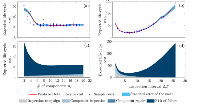
Figure 9: Sample total life-cycle cost with corresponding estimated mean value and standard deviation of the prediction (a-b). The prediction for the cost breakdown is shown in (c-d). There is a slight difference in the prediction of the total cost between (a-b) and (c-d), which comes from the GPR. (a) and (c): varying $n_{I}$ with fixed values {$\Delta T=10$, $p_{th}=1\cdot 10^{-2}$, $\eta=1$}; (b) and (d): varying $\Delta T$ with fixed values {$p_{th}=1\cdot 10^{-2}$, $n_{I}=10$, $\eta=1$}.

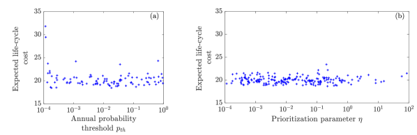
Figure 10: Sample total life-cycle costs, for varying probability threshold $p_{th}$ and prioritization parameter $\eta$. The risk of failure decreases with the probability threshold. However for some values of $p_{th}$ (here lower than $10^{-4}$), the inspection and repair costs needed to satisfy the threshold requirement increase strongly. Probability thresholds that are too small to meet are assigned an arbitrary cost of 1000. (a): $\Delta T=7$, $n_{I}=9$, $\eta=1.3$ (b): $\Delta T=7$, $n_{I}=10$, $p_{th}=5.2\cdot 10^{-3}$.

Figure 11(a) depicts the contours of the GPR surrogate function, as a function of $p_{th}$ and $\eta$, for fixed $\Delta T=7$[years] and $n_{I}=9$. Within a large domain of parameters $p_{th}$ and $\eta$, the surrogate cost varies between $19$ and $21$. Hence the total life-cycle cost is not sensitive to $p_{th}$ and $\eta$ when the values $\Delta T=7$[years] and $n_{I}=9$ are set.

The GPR only provides an approximation of the underlying function; it reports a standard error of 5% on the estimated expected life-cycle cost at the point minimizing the surrogate. To account for this error, we computed 200 additional Monte Carlo samples of deterioration histories and inspection outcomes at the point minimizing the surrogate, which yields an expected total life-cycle cost of $21.4$. We also evaluated 200 Monte Carlo samples for a second strategy, increasing the value of $p_{th}$ by an order of magnitude, i.e. $\{\Delta T=7,\leavevmode\nobreak\ p_{th}=2\cdot 10^{-2},\leavevmode\nobreak\ n_{I}=9,\leavevmode\nobreak\ \eta=1.3\}$. This is motivated by Figure 11(a). For this we obtain an expected total life-cycle cost of $20.1$. Both costs are similar, which confirms that the parameter $p_{th}$ does not considerably affect the expected life-cycle cost of a strategy. Nevertheless, we adopt the latter strategy as the best strategy, $\mathcal{S}_{\bm{w}_{0}^{*}}$, for the prior model, since it gives the smaller expected cost. We highlight the result in Table 2, in which we also include the value given by the surrogate at that point. The corresponding breakdown of the expected total life-cycle cost into its four components is found in Table 3.

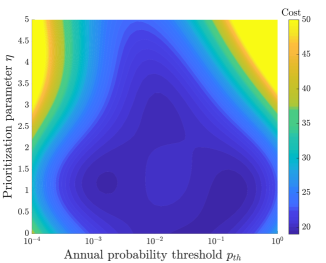
(a)  

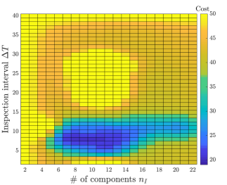
(b)  

Figure 11: (a): Surrogate cost function around the optimum for the prior optimization at $t=0$ for varying heuristic parameters $p_{th}$ (logarithmic scale) and $\eta$, with $\Delta T=7$[years] and $n_{I}=9$. (b): Surrogate cost function around the optimum for the prior optimization at $t=0$ for varying (integer) heuristic parameters $n_{I}$ and $\Delta T$, with $p_{th}=2\cdot 10^{-2}$ and $\eta=1.3$.

Table 2: Parameters $\bm{w}_{0}^{*}$ and expected total life-cycle cost of the optimal strategy at time $t_{0}=0$.

$\Delta T$	$p_{th}$	$n_{I}$	$\eta$	$\mathbf{E}[C_{\text{tot}}|\bm{w}_{0}^{*}]_{MC}$	$\mathbf{E}[C_{\text{tot}}|\bm{w}_{0}^{*}]_{\text{surrogate}}$
$7$	$2\cdot 10^{-2}$	$9$	$1.3$	$20.1$	$20.1$

The Monte Carlo samples also give an estimation of the annual repartition of the cost. Figure 4 shows the expected costs associated with the optimal I&M plan. Notably, the annual risk increases in the years before the first inspection and is progressively reduced with each additional inspection campaign, until it reaches a stationary value.

Table 3: Breakdown of the expected total life-cycle cost for strategy $\mathcal{S}_{\bm{w}_{0}^{*}}$.

Cost component	Expected cost
System failure	$13.0$
Inspection campaign	$3.3$
Component inspection	$3.0$
Component repair	$0.8$

6.3 Adaptive strategy at time $t_{1}=7$ years

The adaptive case is now investigated. Following $\mathcal{S}_{\bm{w}_{0}^{*}}$, the first inspection campaign is carried out at year $t_{1}=7$, with inspections of components {8,9,10,11,16,17,18,19,20}, at a cost of $c_{ini}=9*c_{I}+c_{C}=1.9$. No damage is detected. This information is stored as $\mathbf{z}_{7}$.

At this point, the operator decides to improve the strategy adaptively, rather than continue with strategy $\mathcal{S}_{\bm{w}_{0}^{*}}$.

The optimal strategy $\mathcal{S}_{{\bm{w}_{1}^{*}}_{|\mathbf{z}_{7}}}$ obtained for the posterior model is characterized by the heuristic parameter values in Table 4, with associated expected total life-cycle cost $\mathbf{E}[C_{\text{tot}}|{\bm{w}_{1}^{*}}_{|\mathbf{z}_{7}}]_{\text{surrogate}}=15.9$. This value is discounted to time $t_{1}$, and excludes the initial cost $c_{ini}$.

Table 4: Parameters $\bm{w}_{1}^{*}$ and expected total life-cycle cost of the optimal strategy at time $t_{1}=7$, after no detection of damage on components {8,9,10,11,16,17,18,19,20}.

$\Delta T$	$p_{th}$	$n_{I}$	$\eta$	$\mathbf{E}[C_{\text{tot}}|{\bm{w}_{1}^{*}}_{|\mathbf{z}_{7}}]$
$9$	$3\cdot 10^{-2}$	$9$	$2.2$	15.9

Figures 12(a) and 12(b) depict the contours of the GPR surrogate cost function around the optimum values of the heuristic parameters at time $t_{1}$.

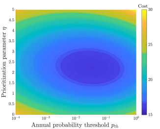
(a)  

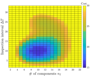
(b)  

Figure 12: (a): Surrogate cost function around the optimum for the adaptive optimization at $t_{1}=7$ for varying heuristic parameters $p_{th}$ (logarithmic scale) and $\eta$, with $\Delta T=9$[years] and $n_{I}=9$. (b): Surrogate cost function around the optimum for the adaptive optimization at $t_{1}=7$ for varying (integer) heuristic parameters $n_{I}$ and $\Delta T$, with $p_{th}=3\cdot 10^{-2}$ and $\eta=2.2$.

The updated optimal heuristic parameters reflect the information gained at time $t_{1}$ and the reduction of uncertainty about the state of the structure. The optimal inspection interval increases to $\Delta T=9$, as does the optimal threshold on the annual probability of system failure, $p_{th}=3\cdot 10^{-2}$. The prescribed number of hotspots to be inspected remains at $n_{I}=9$. Furthermore, the updated prioritization component $\eta$ increases, meaning that it gives more weight to the components’ importance in the system; hence the components with a higher $SEI$ are more likely to be inspected several times during the service life.

In order to compare the initial strategy with the adapted strategy, the expected cost of $\mathcal{S}_{\bm{w}_{0}^{*}}$ conditional on $\mathbf{z}_{7}$ is evaluated with the surrogate cost function. We find that $\mathbf{E}[C_{\text{tot}}|\bm{w}_{0}^{*},\mathbf{z}_{7}]_{\text{surrogate}}=16.9$, excluding the initial cost $c_{ini}$. The expected net gain of changing from strategy $\mathcal{S}_{\bm{w}_{0}^{*}}$ to strategy $\mathcal{S}_{\bm{w}_{1}^{*}}$, after detecting no damage at the first inspection is therefore

$$\mathbf{E}\left[C_{\text{tot}}|\bm{w}_{0}^{*},\mathbf{z}_{7}\right]-\mathbf{E}[C_{tot}|{\bm{w}_{1}^{*}}_{|\mathbf{z}_{7}}]=1.0.$$ (26)

Figure 13 shows that this gain comes from decreasing the number of inspections and repairs, which can be achieved without significantly increasing the risk.

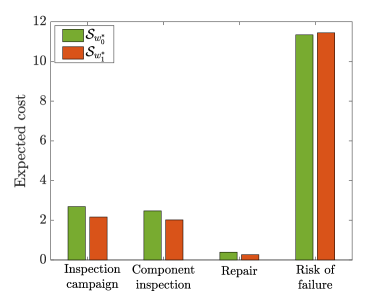
Figure 13: Comparison of expected cost for inspection, repair and failure for strategies $\mathcal{S}_{\bm{w}_{0}^{*}}$ and $\mathcal{S}_{\bm{w}_{1}^{*}}$, conditional on $\mathbf{z}_{7}$.

7 Concluding remarks

In this paper, we present an integral framework for planning inspections and maintenance actions in structural systems. The framework, which draws upon our earlier works (Bismut et al., 2017; Luque and Straub, 2019), for the first time enables such a planning for a general structural system as a whole. It explicitly models deterioration at each component and includes the dependencies among multiple components. It accounts for the interaction among the components within the structural system and their effect on the system reliability. The framework also propagates the information collected at individual component inspections to the rest of the system.

The framework is based on the use of heuristics for prescribing inspection and maintenance strategies. This heuristic approach only results in an approximately optimal strategy. When new information is available, an improved heuristic may be found, which is more optimal under the a-posteriori model. This motivated us to propose an adaptive approach, in which a new optimal heuristic is identified after inspection results are obtained. As we prove in Section 2.2.2, this adapted strategy is always at least as good as the original strategy.

In the investigated numerical application, the adaptation of the strategy results only in limited cost reductions in the order of $5-10\%$. The likely reason for this is that the inspection outcomes are not surprising under the prior model. Were one to consider more unexpected inspection outcomes, the adapted optimal heuristic strategy would differ more significantly from the original strategy.

We introduce a heuristic for prioritizing components for inspections, which is motivated by the value-of-information concept. It accounts for the importance of component in the structural system, but also for the amount of information obtained on other components in the system. Since it is not know a-priori which of these two effects if more important, a heuristic parameter is optimized to weight them. In the future, the heuristic might be adjusted in cases when components are not equi-correlated. Thereby it must be considered that inspections on components with higher correlation are likely to provide more information on the system overall. Simultaneously, it should also be ensured that components are selected for inspections in way that ensures their representativeness for the entire structure. An adjusted heuristic can also account for varying costs of inspections.

In general, the approach is flexible with respect to adding new heuristic rules and parameters. While there is no guarantee that any given heuristic is optimal, the computed expected total life-cycle cost allows to select the best heuristic among the investigated ones. Hence the more heuristics are investigated, the better.

We demonstrate the proposed approach by application to a benchmark problem. There are still challenges to its application in practice. Firstly, setting up the probabilistic model of the structure and the deterioration is non-trivial in many cases. Secondly, the translation of the model to a DBN requires careful calibration of the DBN parameters. The first challenge is shared by all approaches that aim at using physics-based models for predictive maintenance. The second challenge might be addressed by writing corresponding software tools that automatize this task. Alternatively, the DBN could also be replaced by another method that enables fast and efficient Bayesian analysis and reliability updating at the structural system level.

Finally, an extension of the framework to include monitoring data seems straightforward, as long as a Bayesian analysis of the structural system with the monitoring data is possible. Monitoring data can then be treated in the same way as inspection data. With such an extension, the framework can be utilized to optimize monitoring systems.

Appendix A Parameters of the deterioration model

A.1 General model parameters

The parameters of deterioration model are obtained from (Straub, 2009; Luque and Straub, 2016). The relationship between $\text{ln}(C)$ and $M$ is defined after (Ditlevsen and Madsen, 1996), such that the joint distribution of $(\text{ln}(C),M)$ is normally distributed with mean value $(-33,3.5)$, standard deviations $(0.47,0.3)$. Furthermore, we assume a linear relationship between $\text{ln}(C)$ and $M$, implying a correlation coefficient of $-1$, in line with (McCartney and Irving, 1977; Straub, 2004).

A time step $t$ corresponds to $\nu=10^{5}$ fatigue cycles.

For each fatigue hotspots, the stress scale factor $K$ is assumed lognormally distributed. The standard deviation of $\text{ln}(K)$ is $0.22$ for all hotspots, after (Moan and Song, 2000). The mean of $\text{ln}(K)$ varies with the assumed fatigue life for each component (see A.2).

Table 1: Parameters of the fatigue crack growth model.

Variable	Type	Mean	Std. Deviation
$\alpha_{a_{0}}$	Normal dist.	0	1
$\alpha_{K}$	Normal dist.	0	1
$\alpha_{M}$	Normal dist.	0	1
$D_{k,0}$ [mm]	Exponential dist.	1	1
$M_{k}$	Normal dist.	3.5	0.3
$\text{ln}K_{k}$	Normal dist.	Obtained from Table 2	0.22
$\text{ln}(C_{k,i)}$	Function	$\text{ln}(C_{k,i})=-1.5667*M_{k,i}-27.5166$
$\lambda$	Deterministic	$0.8$
$d_{cr}$ [mm]	Deterministic	$50$
$\xi$ [mm]	Deterministic	$10$
$\nu$ [cycles]	Deterministic	$10^{5}$
$T$ [years]	Deterministic	$40$
$\rho_{D_{0}}$	Deterministic	$0.5$
$\rho_{M}$	Deterministic	$0.6$
$\rho_{K}$	Deterministic	$0.8$

A.2 Calibration of the fatigue stress range parameter to the fatigue life

Different approaches for the calibration of deterioration models to the component fatigue design factor (FDF) are discussed in detail in (Straub, 2004). The FDF is defined as the ratio between the component fatigue life, $T_{FL}$, and the system service life, which here is $T_{SL}=T=40$[years]. We calibrate the mean value of the random stress scale parameter $K$ in Equation 23 to the FDF in two steps, so that two damage models coincide in terms of probability of component failure after $T_{SL}$ years.

The first model is the Palmgren-Miner damage accumulation law (Palmgren, 1924; Miner, 1945). For high-cycle fatigue with $n$ stress cycles, the total accumulated damage $\delta_{n}$ is approximated by

$$\delta_{n}=n\cdot\mathbf{E}_{S}\left[\frac{1}{N_{F}(S)}\right],$$ (27)

where $N_{F}$ is the number of cycles to failure at a constant stress amplitude $S$. This relationship, better known as S-N curve, has been defined empirically for various materials, geometries and conditions (Gurney, 1976; Hobbacher, 2015). We adopt the design S-N curve D from the Department of Energy (DoE), UK, after (Straub, 2004). It is assumed that the fatigue stress $S$ has a Weibull distribution with scale parameter $k_{S}$ and shape parameter $\lambda_{S}=0.8$.

Failure occurs when the total damage exceeds a critical threshold, $\Delta$, lognormally distributed with moments $(1,0.3)$ (Faber et al., 2000; JCSS, 2001). The resulting limit state function after $n$ cycles is written:

$$g_{SN}(n)=\Delta-n\cdot\mathbf{E}_{S}\left[\frac{1}{N_{F}(S)}\right].$$ (28)

Additionally, the fatigue life $FDF\cdot T$ is defined such that the total damage reaches the critical value 1, with a yearly cycle rate $\nu$, i.e. $n=\nu\cdot FDF\cdot T$:

$$\nu\cdot FDF\cdot T\cdot\mathbf{E}_{S}\left[\frac{1}{N_{F}(S)}\right]=1.$$ (29)

The expectation in Equation 29 establishes a mapping between FDF and parameter $k_{S}$, depicted in Figure 1(a). Furthermore, for a fixed value of $k_{S}$, the probability of failure at the end of the lifetime $T$, $\text{Pr}\left[g_{SN}(n=\nu\cdot T)<0\right]$, given by the Palmgren-Miner is approximated with FORM (Figure 1(b)). We note that the evaluation of the probability of failure uses the stochastic description of the S-N curve, while the expectation in Equation 29 is computed with the associated characteristic S-N curve.

The second model is the fracture mechanics (FM) model of Equation 22. The limit state function defining failure at time $T$ is written as

$$g_{FM}=d_{cr}-D_{T},$$ (30)

where $D_{T}$ is the crack depth at time $T$, obtained by integration of Equation 22. It is expressed in function of the random variables $K$, $M$ and $D_{0}$ (see Section 5.1). The probability of failure $\text{Pr}\left[g_{FM}<0\right]$ in function of the assumed mean value of $K$, $\mu_{K}$, is shown in Figure 1(c).

Finally, the chosen FDF is mapped to $\mu_{K}$ such that the limit state functions in Equations 30 and 28 result in the same probability of failure at the end of service life $T$. The FDF values and corresponding means of $K$ for all hotspots for the numerical application are obtained by jointly reading Figures 1 (a-c) and are summarized in Table 2.

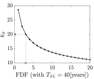
(a)  

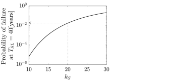
(b)  

(c)  

Figure 1: (a): S-N model parameter $k_{S}$ in function of the FDF. (b): Probability of hotspot failure calculated from the S-N model with parameter $k_{S}$. (c): Probability of hotspot failure according to the FM model, in function of $\mu_{K}$.

Table 2: Fatigue design factors (FDFs) and corresponding mean of random variable $K$ at each hotspot.

Hotspot index $k$	FDF	Mean of $K_{k}$
$\{1,2,3,4\}$	10	$7.58$
$\{5,6,13,14,17,18,21,22\}$	2	$16.26$
$\{7,8,9,10,11,12,19,20\}$	3	$13.29$
$\{15,16\}$	7	$8.88$

Appendix B Estimation of the annual risk of failure

The efficiency of the optimization method described in Section 2.2 depends on the sampling uncertainty of the expectation with MCS (Equation 16), with $n_{MC}=1$ as the limiting case.

In theory, Equation 12 coupled with Equation 16, implies that the probabilities at every time step should be conditioned on the full observation history $\bm{Z}_{1:n_{T}}$, which includes the future inspection outcomes. In this section, we show that one can replace the smoothed probability $\text{Pr}(F_{i}|\bm{w},\bm{Z}_{1:{n_{T}}})$ in Equation 12 by the filtered probability $\text{Pr}(F_{i}|\bm{w},\bm{Z}_{1:{i-1}})$ when estimating the expected risk of failure. Furthermore, we show that the corresponding Monte Carlo estimator of the risk has a smaller sample variance.

We consider the actions that affect the system reliability $\bm{A}=\{A_{1}...A_{n_{T}}\}$ during the service life, such as repair or other maintenance actions. In this paper, the actions are deterministic for given inspection history $\bm{Z}_{1:{n_{T}}}$ and strategy $\mathcal{S}_{\bm{w}}$, i.e. $\bm{A}=\bm{A}(\bm{w},\bm{Z}_{1:{n_{T}}})$. Here we explicitly include them in the expression of the expected cumulative probability of failure:

$$\mathbf{E}_{\bm{Z}_{1:{n_{T}}}}\left[\text{Pr}(F_{i}|\bm{w},\bm{Z}_{1:{n_{T}}})\right]=\mathbf{E}_{\bm{Z}_{1:{n_{T}}}}\left[\text{Pr}(F_{i}|\bm{A}(\bm{w},\bm{Z}_{1:{n_{T}}}),\bm{w},\bm{Z}_{1:{n_{T}}})\right]$$ (31)

We recall two key principles in a sequential decision process. Firstly, a policy at time step $i$ that assigns an action $A_{i}$ can only consider information $\bm{Z}_{1:{i}}$ about the system up to that time, or in other terms, decisions cannot be based on specific knowledge acquired in the future, i.e. $A_{i}=A_{i}(\bm{w},\bm{Z}_{1:{i}})$. Secondly, the cumulative failure event $F_{i}$ never depends on the actions after time step $i$, $\bm{A}_{i:n_{T}}$, neither unconditionally nor conditionally on $\bm{Z}_{1:{n_{T}}}$. Hence we obtain Equation 32:

$$\begin{split}\mathbf{E}_{\bm{Z}_{1:{n_{T}}}}\left[\text{Pr}(F_{i}|\bm{w},\bm{Z}_{1:{n_{T}}})\right]&=\mathbf{E}_{\bm{Z}_{1:{n_{T}}}}\left[\text{Pr}(F_{i}|\bm{A}_{1:{i-1}}(\bm{w},\bm{Z}_{1:{i-1}}),\bm{w},\bm{Z}_{1:{n_{T}}})\right]\end{split}$$ (32)

From there, we can split the expectation of the right hand term of Equation 32:

$$\begin{split}\mathbf{E}_{\bm{Z}_{1:{n_{T}}}}\left[\text{Pr}(F_{i}|\bm{w},\bm{Z}_{1:{n_{T}}})\right]&=\mathbf{E}_{\bm{Z}_{1:{i-1}}}\left[\mathbf{E}_{\bm{Z}_{{i}:n_{T}}|{\bm{Z}_{1:{i-1}}}}\left[\text{Pr}(F_{i}|\bm{A}_{1:{i-1}}(\bm{w},\bm{Z}_{1:{i-1}}),\bm{w},\bm{Z}_{1:{i-1}},\bm{Z}_{{i}:n_{T}})\right]\right]\\ &=\mathbf{E}_{\bm{Z}_{1:{i-1}}}\left[\text{Pr}(F_{i}|\bm{A}_{1:{i-1}}(\bm{w},\bm{Z}_{1:{i-1}}),\bm{w},\bm{Z}_{1:{i-1}})\right].\end{split}$$ (33)

Finally we obtain,

$$\begin{split}\mathbf{E}_{\bm{Z}_{1:{n_{T}}}}\left[\text{Pr}(F_{i}|\bm{w},\bm{Z}_{1:{n_{T}}})\right]&=\mathbf{E}_{\bm{Z}_{1:{i-1}}}\left[\text{Pr}(F_{i}|\bm{w},\bm{Z}_{1:{i-1}})\right].\end{split}$$ (34)

Therefore for a sample observation history $\mathbf{z}_{1:{n_{T}}}$, the conditional filtered probability, $\text{Pr}(F_{i}|\bm{w},\mathbf{z}_{1:{i-1}})$, and the smoothed probability, $\text{Pr}(F_{i}|\bm{w},\mathbf{z}_{1:{n_{T}}})$, are two valid unbiased estimators of the expected value $\mathbf{E}_{\bm{Z}_{1:{n_{T}}}}\left[\text{Pr}(F_{i}|\bm{w},\bm{Z}_{1:{n_{T}}})\right]$. Furthermore, Equation 33 shows that the filtered probability is equal to the expectation of the smoothed probability over the inspection results $\bm{Z}_{i:n_{T}}$. This implies that the filtered probability is an estimator with a smaller variance than the smoothed probability, hence is better suited as estimator of the noisy objective function in the optimization method described in Section 2.2.

The variances of these two estimator and the standard error of the mean can be compared for the I&M strategies that prescribe only inspections but no repair or maintenance actions to be carried out, i.e. for any $\bm{Z}_{1:{n_{T}}}$, and at any time step $i$, $A_{i}(\bm{Z}_{1:i})=\textit{`do nothing'}$. For instance, the strategy parametrized by $\bm{w}=\{\Delta T=10,p_{th}=1,n_{i}=5,\eta=1,D_{rep}=\infty\}$ satisfies this condition. The expectations $\mathbf{E}_{\bm{Z}_{1:{i-1}}}\left[\text{Pr}(F_{i}|\bm{w},\bm{Z}_{1:{i-1}})\right]$ and $\mathbf{E}_{\bm{Z}_{1:{n_{T}}}}\left[\text{Pr}(F_{i}|\bm{w},\bm{Z}_{1:{n_{T}}})\right]$ are equal to $\text{Pr}(F_{i})$ calculated with the prior model assumptions. The variance of these estimators is evaluated for the numerical application described in Section 5, with $n_{MC}=500$ sample histories (see Figure 2).

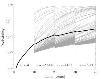
(a)  

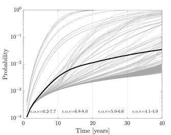
(b)  

Figure 2: Strategy defined by $\bm{w}=\{\Delta T=10,p_{th}=1,n_{i}=5,\eta=1,D_{rep}=\infty\}$. (a): Filtered conditional probability of failure $\text{Pr}(F_{i}|\bm{w},\bm{Z}_{1:{i-1}})$ for $500$ sample histories $\bm{z}^{(q)}$, and resulting mean (bold line); (b) Smoothed conditional probability of failure $\text{Pr}(F_{i}|\bm{w},\bm{Z}_{1:n_{T}})$ for $500$ sample histories $\bm{z}^{(q)}$, and resulting mean (bold line). The estimated range of the coefficient of variation (c.o.v) is indicated for each decade.

The variance of the smoothed estimator is indeed larger than of the filtered estimator: for the times between $1$ and $10$ years, the filtered estimator is exact, and the coefficient of variation of the smoothed estimator is of the order of 500%. For the subsequent time steps, up to year $30$, the coefficient of variation of the smoothed estimator is up to 1.3 times that of the filtered estimator.

Appendix C Prioritization Index for component inspection

The Prioritization Index (PI) is chosen as a proxy for the VoI. The reasoning behind the expression for the PI in Equation 21 is outlined in this section. Here $F_{s}$ is used to denote the event $F_{i}^{*}$ for a given time step $i$. The following derivations omit the conditioning on $\bm{Z}_{1:{i-1}}$. The $SEI_{k}$ are nonetheless independent of any observation, by definition.

We express the certain event as $\{\Omega\}=\{\{F_{c_{1}}\cup\overline{F_{c_{1}}}\}\cap...\cap\{F_{c_{N}}\cup\overline{F_{c_{N}}}\}\}$, and obtain that

$$\begin{split}\text{Pr}(F_{s})=\leavevmode\nobreak\ &\text{Pr}(F_{s}\cap\{\{F_{c_{1}}\cup\overline{F_{c_{1}}}\}\cap...\cap\{F_{c_{N}}\cup\overline{F_{c_{N}}}\}\})\\ =\leavevmode\nobreak\ &\text{Pr}(F_{s},\overline{F_{c_{1}}},...,\overline{F_{c_{N}}})+\text{Pr}(F_{s},F_{c_{1}},\overline{F_{c_{2}}},...,\overline{F_{c_{N}}})+\text{Pr}(F_{s},\overline{F_{c_{1}}},F_{c_{2}},...\overline{F_{c_{N}}})\\ &+...+\text{Pr}(F_{s},\overline{F_{c_{1}}},\overline{F_{c_{2}}},...,\overline{F_{c_{N-1}}},F_{c_{N}})+{\sum_{\mathcal{I}}{\text{Pr}(F_{s},{F_{c_{\mathcal{I}}}}\cap{\overline{F_{c_{\smallsetminus\mathcal{I}}}}})}}\\ \end{split}$$ (35)

The last term in Equation 35 corresponds to the joint probabilities of $F_{s}$ and failed components belonging to the subsets $\mathcal{I}$ of $\{1..N\}$, with $|\mathcal{I}|\geq 2$.

By introducing conditional probabilities and writing $a=\text{Pr}(F_{s}|\overline{F_{c_{1}}},...,\overline{F_{c_{N}}})$, the probability of failure of the system is

$$\begin{split}\text{Pr}(F_{s})=&\leavevmode\nobreak\ a\cdot\text{Pr}(\overline{F_{c_{1}}},...,\overline{F_{c_{N}}})+\text{Pr}(F_{s}|F_{c_{1}},\overline{F_{c_{2}}},...,\overline{F_{c_{N}}})\cdot\text{Pr}(F_{c_{1}},\overline{F_{c_{2}}},...,\overline{F_{c_{N}}})+...+\\ &\text{Pr}(F_{s}|\overline{F_{c_{1}}},\overline{F_{c_{2}}},...F_{c_{N}})\cdot\text{Pr}(\overline{F_{c_{1}}},\overline{F_{c_{2}}},...F_{c_{N}})+{\sum_{\mathcal{I}}{\text{Pr}(F_{s}|{F_{c_{\mathcal{I}}}}\cap{\overline{F_{c_{\smallsetminus\mathcal{I}}}}})\cdot\text{Pr}({F_{c_{\mathcal{I}}}}\cap{\overline{F_{c_{\smallsetminus\mathcal{I}}}}})}}\\ \end{split}$$ (36)

From Equation 20, we have that $\text{Pr}(F_{s}|\overline{F_{c_{1}}},...,\overline{F_{c_{k-1}}},F_{c_{k}},\overline{F_{c_{k+1}}},...,\overline{F_{c_{N}}})=a+SEI_{k}$, and similarly we can express each $\text{Pr}(F_{s}|{F_{c_{\mathcal{I}}}}\cap{\overline{F_{c_{\smallsetminus\mathcal{I}}}}})=a+MEI_{\mathcal{I}}$, where $MEI_{\mathcal{I}}$ is the multiple elements importance of components in $\mathcal{I}$. By factorizing $a$, we obtain Equation 37:

$$\begin{split}\text{Pr}(F_{s})=&\leavevmode\nobreak\ a+SEI_{1}\cdot\text{Pr}(F_{c_{1}},\overline{F_{c_{2}}},...,\overline{F_{c_{N}}})+...\\ &+SEI_{N}\cdot\text{Pr}(\overline{F_{c_{1}}},\overline{F_{c_{2}}},...F_{c_{N}})+b,\end{split}$$ (37)

where $b$ represents the contribution of simultaneous component failures. Equation 38 introduces the marginal probabilities of component failure:

$$\begin{split}\text{Pr}(F_{s})=&\leavevmode\nobreak\ a+SEI_{1}\cdot\text{Pr}(F_{c_{1}})\cdot\text{Pr}(\overline{F_{c_{2}}},...,\overline{F_{c_{N}}}|F_{c_{1}})\\ &+...+SEI_{N}\cdot\text{Pr}(F_{c_{N}})\cdot\text{Pr}(\overline{F_{c_{1}}},...,\overline{F_{c_{N-1}}}|F_{c_{N}})+b.\end{split}$$ (38)

From Equation 38, we approximate $\text{Pr}(F_{s})$ with

$$\text{Pr}(F_{s})\simeq a+SEI_{1}\cdot\text{Pr}(F_{c_{1}})+...+SEI_{N}\cdot\text{Pr}(F_{c_{N}})+b,$$ (39)

Equation 39 is not actually used to calculate the interval failure probability of the system, $\text{Pr}(F_{i}^{*})$, but shows that the probability of system failure approximately is a function of the terms $SEI_{k}\cdot\text{Pr}(F_{c_{k}})$ defined for each component, hence by the VoI for component $k$ is a linear function of $SEI_{k}\cdot\text{Pr}(F_{c_{k}})$. Furthermore, the amount of information learnt on other components is related to the probability of failure $\text{Pr}(F_{c_{k}})$, through the components’ interdependence.

Figure 3 compares two sample inspection histories for two values of $\eta$, from the numerical application to the Zayas frame. As expected, more hotspots are inspected during the service life when a lower value for $\eta$ is fixed. For a higher value of $\eta$ the inspected hotspots are principally those with the higher $SEI$ values.

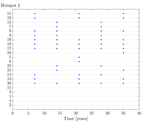
(a) $\eta=0.84$

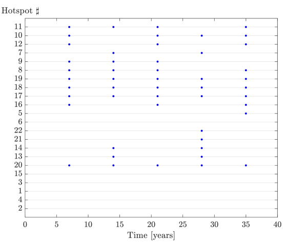
(b) $\eta=2.96$

Figure 3: History of hotspots inspected (marked with a blue dot) for a sample deterioration history, following the strategies defined by $\Delta T=7$[years], $n_{I}=10$ and $p_{th}=5.2\cdot 10^{-3}$, and a lower (a) and higher (b) prioritization parameter $\eta$. The hotspots numbers on the y-axis are sorted according to their calculated $SEI$.

References

- Andriotis and Papakonstantinou (2019) Andriotis, C., Papakonstantinou, K., 2019. Managing engineering systems with large state and action spaces through deep reinforcement learning. Reliability Engineering & System Safety 191, 106483.
- Askar and Derin (1981) Askar, M., Derin, H., 1981. A recursive algorithm for the bayes solution of the smoothing problem. IEEE Transactions on Automatic Control 26 (2), 558–561.
- Askar and Derin (1983) Askar, M., Derin, H., 1983. Recursive algorithms for the bayes solution of the fixed-point and fixed-lag smoothing problems. IEEE Transactions on Automatic Control 28 (10), 996–998.
- Åström (1965) Åström, K. J., 1965. Optimal control of Markov processes with incomplete state information. Journal of mathematical analysis and applications 10 (1), 174–205.
- Barlow and Hunter (1960) Barlow, R., Hunter, L., 1960. Optimum preventive maintenance policies. Operations research 8 (1), 90–100.
- Barone and Frangopol (2014) Barone, G., Frangopol, D. M., 2014. Reliability, risk and lifetime distributions as performance indicators for life-cycle maintenance of deteriorating structures. Reliability Engineering & System Safety 123, 21–37.
- Bellman (1957a) Bellman, R., 1957a. Dynamic Programming. Princeton University Press.
- Bellman (1957b) Bellman, R., 1957b. A Markovian decision process. Journal of Mathematics and Mechanics 6 (5), 679–684.
- Bismut et al. (2017) Bismut, E., Luque, J., Straub, D., 2017. Optimal prioritization of inspections in structural systems considering component interactions and interdependence. In: 12th International Conference on Structural Safety & Reliability, ICOSSAR 2017. pp. 2260–2269.
- Bocchini et al. (2013) Bocchini, P., Saydam, D., Frangopol, D. M., 2013. Efficient, accurate, and simple Markov chain model for the life-cycle analysis of bridge groups. Structural Safety 40, 51–64.
- Chebotar et al. (2017) Chebotar, Y., Kalakrishnan, M., Yahya, A., Li, A., Schaal, S., Levine, S., 2017. Path integral guided policy search. In: Robotics and Automation (ICRA), 2017 IEEE International Conference on. IEEE, pp. 3381–3388.
- Chen and Lee (2011) Chen, C.-h., Lee, L. H., 2011. Stochastic simulation optimization: an optimal computing budget allocation. Vol. 1. World scientific.
- Chen and Sohal (1988) Chen, W.-F., Sohal, I., 1988. Cylindrical members in offshore structures. Thin-Walled Structures 6 (3), 153–285.
- De Boer et al. (2005) De Boer, P.-T., Kroese, D. P., Mannor, S., Rubinstein, R. Y., 2005. A tutorial on the cross-entropy method. Annals of operations research 134 (1), 19–67.
- de Jonge et al. (2017) de Jonge, B., Teunter, R., Tinga, T., 2017. The influence of practical factors on the benefits of condition-based maintenance over time-based maintenance. Reliability Engineering & System Safety 158, 21–30.
- Ditlevsen and Madsen (1996) Ditlevsen, O., Madsen, H. O., 1996. Structural reliability methods. Vol. 178. Wiley New York.
- Durango and Madanat (2002) Durango, P. L., Madanat, S. M., 2002. Optimal maintenance and repair policies in infrastructure management under uncertain facility deterioration rates: an adaptive control approach. Transportation Research Part A: Policy and Practice 36 (9), 763–778.
- Efroni et al. (2018) Efroni, Y., Dalal, G., Scherrer, B., Mannor, S., 2018. Multiple-step greedy policies in approximate and online reinforcement learning. In: Advances in Neural Information Processing Systems. pp. 5238–5247.
- Enright and Frangopol (1999) Enright, M. P., Frangopol, D. M., 1999. Condition prediction of deteriorating concrete bridges using Bayesian updating. Journal of Structural Engineering 125 (10), 1118–1125.
- Faber et al. (2000) Faber, M. H., Engelund, S., Sørensen, J. D., Bloch, A., 2000. Simplified and generic risk based inspection planning. In: Proceedings of OMAE2000, New Orleans, 2000. Paper 6143.
- Faddoul et al. (2013) Faddoul, R., Soubra, A. H., Raphael, W., Chateauneuf, A., 2013. Extension of dynamic programming models for management optimisation from single structure to multi-structures level. Structure and Infrastructure Engineering 9 (5), 432–447.
- Grall et al. (2002) Grall, A., Dieulle, L., Bérenguer, C., Roussignol, M., 2002. Continuous-time predictive-maintenance scheduling for a deteriorating system. IEEE transactions on reliability 51 (2), 141–150.
- Gurney (1976) Gurney, T. R., 1976. Fatigue design rules for welded steel joins. Welding Institute Research Bulletin 17, 115–124.
- He et al. (2010) He, D., Lee, L. H., Chen, C.-H., Fu, M. C., Wasserkrug, S., 2010. Simulation optimization using the cross-entropy method with optimal computing budget allocation. ACM Transactions on Modeling and Computer Simulation (TOMACS) 20 (1), 4.
- Hill (2013) Hill, S. D., 2013. Discrete optimization with noisy objective function measurements. Wiley Encyclopedia of Operations Research and Management Science.
- Hobbacher (2015) Hobbacher, A., 2015. Recommendations for fatigue design of welded joints and components. Springer.
- Howard (1960) Howard, R. A., 1960. Dynamic programming and Markov Processes. Technology Press and Wiley New York.
- Irving and McCartney (1977) Irving, P., McCartney, L., 1977. Prediction of fatigue crack growth rates: theory, mechanisms, and experimental results. Metal Science 11 (8-9), 351–361.
- JCSS (2001) JCSS, J., 2001. Probabilistic model code. Joint Committee on Structural Safety.
- Jensen et al. (2007) Jensen, F. V., Nielsen, T. D., Nielsen, T. D., 2007. Bayesian Networks and Decision Graphs, 2nd Edition. Information Science and Statistics. Springer New York.
- Kaelbling et al. (1998) Kaelbling, L. P., Littman, M. L., Cassandra, A. R., 1998. Planning and acting in partially observable stochastic domains. Artificial intelligence 101 (1-2), 99–134.
- Kahn et al. (2017) Kahn, G., Zhang, T., Levine, S., Abbeel, P., 2017. Plato: Policy learning using adaptive trajectory optimization. In: 2017 IEEE International Conference on Robotics and Automation (ICRA). pp. 3342–3349.
- King (1998) King, R., 1998. A review of fatigue crack growth rates in air and seawater. Health and Safety Executive Norwich, UK.
- Kochenderfer (2015) Kochenderfer, M. J., 2015. Decision making under uncertainty: theory and application. MIT press.
- Kübler and Faber (2004) Kübler, O., Faber, M. H., 2004. Optimality and acceptance criteria in offshore design. Journal of Offshore Mechanics and Arctic Engineering 126 (3), 258–264.
- Lam and Yeh (1994) Lam, C. T., Yeh, R. H., 1994. Optimal maintenance-policies for deteriorating systems under various maintenance strategies. IEEE Transactions on reliability 43 (3), 423–430.
- Lin and Yang (1985) Lin, Y. K., Yang, J. N., 1985. A stochastic theory of fatigue crack propagation. AIAA journal 23 (1), 117–124.
- Luque and Straub (2013) Luque, J., Straub, D., 2013. Algorithms for optimal risk-based planning of inspections using influence diagrams. In: Proceedings of the 11th International Probabilistic Workshop.
- Luque and Straub (2016) Luque, J., Straub, D., 2016. Reliability analysis and updating of deteriorating systems with dynamic Bayesian networks. Structural Safety 62, 34–46.
- Luque and Straub (2019) Luque, J., Straub, D., 2019. Risk-based optimal inspection strategies for structural systems using dynamic Bayesian networks. Structural Safety 76, 68–80.
- Madsen et al. (1987) Madsen, H., Skjong, R., Tallin, A., 1987. Probabilistic fatigue crack growth analysis of offshore structures, with reliability updating through inspection. In: Marine Structural Reliability Engineering Symposium.
- McCartney and Irving (1977) McCartney, L., Irving, P., 1977. Comments on: "A correlation for fatigue crack growth rate". Scripta Metallurgica 11 (3), 181–183.
- Melchers (2003) Melchers, R., 2003. Modeling of marine immersion corrosion for mild and low-alloy steels—part 1: Phenomenological model. Corrosion 59 (4), 319–334.
- Memarzadeh and Pozzi (2016) Memarzadeh, M., Pozzi, M., 2016. Value of information in sequential decision making: component inspection, permanent monitoring and system-level scheduling. Reliability Engineering & System Safety 154, 137–151.
- Miner (1945) Miner, M. A., 1945. Cumulative fatigue damage. Journal of applied mechanics 12 (3), A159–A164.
- Moan (2005) Moan, T., 2005. Reliability-based management of inspection, maintenance and repair of offshore structures. Structure and Infrastructure Engineering 1 (1), 33–62.
- Moan and Song (2000) Moan, T., Song, R., 2000. Implications of inspection updating on system fatigue reliability of offshore structures. Journal of Offshore Mechanics and Arctic Engineering 122 (3), 173–180.
- Newman Jr (1998) Newman Jr, J., 1998. The merging of fatigue and fracture mechanics concepts: a historical perspective. Progress in Aerospace Sciences 34 (5-6), 347–390.
- Ng et al. (2000) Ng, A. Y., Parr, R., Koller, D., 2000. Policy search via density estimation. In: Advances in Neural Information Processing Systems. pp. 1022–1028.
- Nielsen and Sørensen (2010a) Nielsen, J. J., Sørensen, J. D., 2010a. Bayesian networks as a decision tool for O&M of offshore wind turbines. In: Proceedings of the 5th international ASRANet conference.
- Nielsen and Sørensen (2010b) Nielsen, J. J., Sørensen, J. D., 2010b. Risk-based operation and maintenance planning for offshore wind turbines. In: Proceedings of the Reliability and Optimization of Structural Systems. pp. 7–10.
- Nielsen and Sørensen (2014) Nielsen, J. S., Sørensen, J. D., 2014. Methods for risk-based planning of O&M of wind turbines. Energies 7 (10), 6645–6664.
- Nielsen and Sørensen (2015) Nielsen, J. S., Sørensen, J. D., 2015. Risk-based decision making for deterioration processes using POMDP. In: ICASP12 International Conference on Applications of Statistics and Probability in Civil Engineering.
- Palmgren (1924) Palmgren, A., 1924. Die lebensdauer von kugellagern. Zeitschrift des Vereines Deutscher Ingenieure 68 (4), 339–341.
- Papadimitriou and Tsitsiklis (1987) Papadimitriou, C. H., Tsitsiklis, J. N., 1987. The complexity of Markov decision processes. Mathematics of operations research 12 (3), 441–450.
- Papakonstantinou et al. (2018) Papakonstantinou, K. G., Andriotis, C. P., Shinozuka, M., 2018. POMDP and MOMDP solutions for structural life-cycle cost minimization under partial and mixed observability. Structure and Infrastructure Engineering 14 (7), 869–882.
- Papakonstantinou and Shinozuka (2014) Papakonstantinou, K. G., Shinozuka, M., 2014. Optimum inspection and maintenance policies for corroded structures using partially observable Markov decision processes and stochastic, physically based models. Probabilistic Engineering Mechanics 37, 93–108.
- Pineau et al. (2006) Pineau, J., Gordon, G., Thrun, S., 2006. Anytime point-based approximations for large POMDP. Journal of Artificial Intelligence Research 27, 335–380.
- Pooya and Pakdaman (2018) Pooya, A., Pakdaman, M., 2018. Optimal control model for finite capacity continuous MRP with deteriorating items. Journal of Intelligent Manufacturing 30 (5), 1–13.
- Powell (2011) Powell, W. B., 2011. Approximate Dynamic Programming : Solving the Curses of Dimensionality. John Wiley & Sons, Incorporated, Hoboken, United States.
- Raiffa and Schlaifer (1961) Raiffa, H., Schlaifer, R., 1961. Applied Statistical Decision Theory. Harvard Business Review Press.
- Rasmussen (2004) Rasmussen, C. E., 2004. Gaussian processes in machine learning. Springer, pp. 63–71.
- Rausand and Høyland (2004) Rausand, M., Høyland, A., 2004. System reliability theory: models, statistical methods, and applications. Vol. 396. John Wiley & Sons.
- Röckmann et al. (2017) Röckmann, C., Lagerveld, S., Stavenuiter, J., 2017. Operation and Maintenance Costs of Offshore Wind Farms and Potential Multi-use Platforms in the Dutch North Sea. Springer International Publishing, Cham, pp. 97–113.
- Rosenfield (1976) Rosenfield, D., 1976. Markovian deterioration with uncertain information—a more general model. Naval Research Logistics Quarterly 23 (3), 389–405.
- Rosenstein and Barto (2001) Rosenstein, M. T., Barto, A. G., 2001. Robot weightlifting by direct policy search. In: International Joint Conference on Artificial Intelligence. Vol. 17. Citeseer, pp. 839–846.
- Rubinstein and Kroese (2004) Rubinstein, R. Y., Kroese, D. P., 2004. The cross-entropy method: a unified approach to combinatorial optimization, Monte-Carlo simulation and machine learning. Springer Science & Business Media.
- Rubinstein and Kroese (2017) Rubinstein, R. Y., Kroese, D. P., 2017. Simulation and the Monte Carlo method, 3rd Edition. Wiley series in probability and statistics. Wiley, Hoboken, New Jersey.
- Schneider (2019) Schneider, R., 2019. Effect of repair models on risk based optimal inspection strategies for support structures of offshore wind turbines.
- Schneider et al. (2017) Schneider, R., Thöns, S., Straub, D., 2017. Reliability analysis and updating of deteriorating systems with subset simulation. Structural Safety 64, 20–36.
- Schöbi and Chatzi (2016) Schöbi, R., Chatzi, E. N., 2016. Maintenance planning using continuous-state partially observable Markov decision processes and non-linear action models. Structure and Infrastructure Engineering 12 (8), 977–994.
- Shafiee et al. (2015) Shafiee, M., Finkelstein, M., Bérenguer, C., 2015. An opportunistic condition-based maintenance policy for offshore wind turbine blades subjected to degradation and environmental shocks. Reliability Engineering & System Safety 142, 463–471.
- Silver and Veness (2010) Silver, D., Veness, J., 2010. Monte-carlo planning in large POMDPs. In: Advances in neural information processing systems. pp. 2164–2172.
- Southwell et al. (1979) Southwell, C., Bultman, J., Hummer, C., 1979. Estimating service life of steel in seawater. Seawater corrosion handbook 87, 374.
- Spall (2012) Spall, J. C., 2012. Stochastic optimization. In: Handbook of computational statistics. Springer, pp. 173–201.
- Straub (2004) Straub, D., 2004. Generic approaches to risk based inspection planning for steel structures. Vol. 284. vdf Hochschulverlag AG.
- Straub (2009) Straub, D., 2009. Stochastic modeling of deterioration processes through dynamic Bayesian networks. Journal of Engineering Mechanics 135 (10), 1089–1099.
- Straub and Der Kiureghian (2011) Straub, D., Der Kiureghian, A., 2011. Reliability acceptance criteria for deteriorating elements of structural systems. Journal of Structural Engineering 137 (12), 1573–1582.
- Straub and Faber (2005) Straub, D., Faber, M. H., 2005. Risk based inspection planning for structural systems. Structural safety 27 (4), 335–355.
- Straub and Faber (2006) Straub, D., Faber, M. H., 2006. Computational aspects of risk-based inspection planning. Computer-Aided Civil and Infrastructure Engineering 21 (3), 179–192.
- Straub and Papaioannou (2015) Straub, D., Papaioannou, I., 2015. Bayesian updating with structural reliability methods. Journal of Engineering Mechanics 141 (3), 04014134.
- Straub et al. (2020) Straub, D., Schneider, R., Bismut, E., Kim, H.-J., 2020. Reliability analysis of deteriorating structural systems. Structural Safety 82, 101877.
- Sutton et al. (2000) Sutton, R. S., McAllester, D. A., Singh, S. P., Mansour, Y., 2000. Policy gradient methods for reinforcement learning with function approximation. In: Advances in neural information processing systems. pp. 1057–1063.
- Särkkä (2013) Särkkä, S., 2013. Bayesian filtering and smoothing. Vol. 3. Cambridge University Press.
- Thoft-Christensen and Sørensen (1987) Thoft-Christensen, P., Sørensen, J., 1987. Optimal strategy for inspection and repair of structural systems. Civil Engineering Systems 4 (2), 94–100.
- Tsang (1995) Tsang, A. H., 1995. Condition-based maintenance: tools and decision making. Journal of quality in maintenance engineering 1 (3), 3–17.
- van Noortwijk (2009) van Noortwijk, J. M., 2009. A survey of the application of gamma processes in maintenance. Reliability Engineering & System Safety 94 (1), 2–21.
- Wirsching and Chen (1988) Wirsching, P. H., Chen, Y. N., 1988. Considerations of probability-based fatigue design for marine structures. Marine Structures 1 (1), 23–45.
- Yang (1994) Yang, J., 1994. Application of reliability methods to fatigue, quality assurance and maintenance. In: Proceedings of ICOSSAR’93, Innsbruck. pp. 1–21.
- Zayas (1980) Zayas, V. A., 1980. Ultimate earthquake resistance of steel offshore structures. Thesis.
- Zhu and Collette (2015) Zhu, J., Collette, M., 2015. A dynamic discretization method for reliability inference in dynamic bayesian networks. Journal of Reliability Engineering System Safety 138, 242–252.
- Zhu et al. (2013) Zhu, W., Fouladirad, M., Bérenguer, C., 2013. A predictive maintenance policy based on the blade of offshore wind turbine. In: IEEE Proceedings of Reliability and Maintainability Symposium (RAMS). pp. 1–6.