Predicting Sunspot Numbers for Solar Cycles 25 and 26

Abstract

The prediction of solar activity is important for advanced technologies and space activities. The peak sunspot number (SSN), which can represent the solar activity, has declined continuously in the past four solar cycles (21$-$24), and the Sun would experience a Dalton-like minimum, or even the Maunder-like minimum, if the declining trend continues in the following several cycles, so that the predictions of solar activity for cycles 25 and 26 are crucial. In Qin & Wu, 2018, ApJ, we established an SSN prediction model denoted as two-parameter modified logistic prediction (TMLP) model, which can predict the variation of SSNs in a solar cycle if the start time of the cycle has been determined. In this work, we obtain a new model denoted as TMLP-extension (TMLP-E), . It is found that the predicted solar maximum, ascent time, and cycle length are 115.1, 4.84 yr, and 11.06 yr, respectively, for cycle 25, and 107.3, 4.80 yr, and 10.97 yr, respectively, for cycle 26. The solar activities of cycles 25 and 26 are predicted to be at the same level as that of cycle 24, but will not decrease further. We therefore suggest that the cycles 24$-$26 are at a minimum of Gleissberg cycle.

1 Introduction

The solar activity has vital influences on the solar-terrestrial environment, which further affects the health of human beings and the safety of spacecraft as well as the reliability of navigation and communication (e.g., Lanzerotti, 2017; Mertens et al., 2018; Shen & Qin, 2018; Wu & Qin, 2018). Most of solar activities range from several minutes to decadal-scale, such as the quasi-11-year period of solar activity strength, which is called the solar activity cycle and can be well represented by the sunspot number (SSN) (e.g., Balogh et al., 2014; Hathaway, 2015; Lin et al., 2019; Petrovay, 2020; Chen et al., 2021).

Long-term predictions of solar activity are essential for planning future space missions and understanding the underlying mechanism of the solar cycle. The predictions for solar cycles 25 and 26 are more crucial because the solar maximum, defined as the peak monthly smoothed SSN of a solar cycle, has declined continuously in the past 4 cycles (21$-$24). Solar cycle 24 is the second lowest cycle with the solar maximum being 116.4 since the Dalton minimum, recorded around the year 1810. A new Dalton-like minimum even the Maunder-like minimum may occur if the solar activity decreases further in cycles 25 and 26, which will cause some important space weather effects.

A lot of research has been focused on the prediction of the solar maximum of cycle 25 in recent years. Firstly, some research suggested that the declining trend of solar activity will continue. The solar maximum of cycle 25 is predicted to be about 14% (Macario-Rojas et al., 2018), 24% (Labonville et al., 2019), and 31% (Singh et al., 2019) lower than that of cycle 24. In addition, several works obtained much lower values, e.g., 50 $\pm$ 15 (Kitiashvili, 2020) and 57 $\pm$ 17 (Covas et al., 2019), for the solar maximum of cycle 25, which indicates that cycle 25 would be the weakest cycle since the Maunder minimum (1645$-$1715; e.g., Eddy, 1976). Secondly, some other studies, however, inferred that the declining trend of solar activity will break and cycle 25 would be stronger than cycle 24. The solar maximum of cycle 25 is forecast to be about 16% (Pesnell & Schatten, 2018), 24% (Kakad et al., 2020), 30% (Du, 2020), 32% (Sarp et al., 2018), and 45% (Li et al., 2018) greater than that of cycle 24. A pretty large value of 228.8 $\pm$ 40.5 was suggested by Han & Yin (2019). Finally, there are also some works to predict that the solar maximum of cycle 25 would be similar to that of cycle 24 (the difference is within 10%) (e.g., Bhowmik & Nandy, 2018; Jiang et al., 2018; Okoh et al., 2018; Upton & Hathaway, 2018; Gonçalves et al., 2020; Lee, 2020).

Compared with the cycle 25, researchers seldom work on the predictions for the cycle 26 since longer term forecasts are more difficult. Charvátová (2009) suggested that cycles 24$-$26 would be a repeat of cycles 11$-$13, so that the solar maxima of cycles 24$-$26 should be 140.3, 74.6, and 87.9, respectively. Hiremath (2008) forecasted the amplitude and period of cycles 24$-$38. The solar maximum was predicted to be 110 $\pm$ 11 for both cycle 24 and cycle 25, while cycle 26 was supposed to experience a very high solar activity. Note that, these early predictions are made based on the Version 1.0 SSN as the Version 2.0 SSN was not released until 2015 (Clette et al., 2015; Clette & Lefèvre, 2016). The observed solar activity of cycle 24, however, is at a relatively low level with the solar maximum being 81.9 for the Version 1.0 SSN. Abdusamatov (2007) predicted that the solar maxima of cycles 24, 25, and 26 would be 70 $\pm$ 10, 50 $\pm$ 15, and 35 $\pm$ 20, respectively, for the Version 1.0 SSN. Singh & Bhargawa (2019) also predicted that the declining trend of solar activity would continue with the solar maxima of cycles 25 and 26 being 89 $\pm$ 9 and 78 $\pm$ 7, respectively, for the Version 2.0 SSN. They suggested that the Sun would experience a Dalton-like minimum by the year 2043. In Javaraiah (2017), a low value of 30$-$40 for cycles 25 and 26 was predicted, and the epochs of cycles 25 and 26 were suggested to be at a minimum of Gleissberg cycle, which is a 60$-$120 yr variation in solar cycle amplitude (e.g., Gleissberg, 1939; Petrovay, 2020).

It is shown that the solar maximum of cycle 25 predicted by various methods ranges from a pretty low value of 50 up to a very large value of 228.8 Pesnell (2016) showed that 105 predictions for cycle 24 also gave a wide prediction range. Besides, predictions for cycle 26 are rare so far,

Recently, we established an SSN prediction model, denoted as two-parameter modified logistic prediction (hereafter referred to as TMLP) model (Qin & Wu, 2018), statistically. The model can predict the variation of SSNs in a solar cycle when the start time of the cycle has been determined. we obtain a new model denoted as TMLP-extension (hereafter referred to as TMLP-E) by extending the prediction ability of TMLP . If the start time of a cycle $n$ is already known, TMLP-E can predict the variation of SSNs in the cycle $n+1$. In September 2020, the SILSO World Data center confirmed that cycle 25 started in December 2019 (see http://sidc.be/silso/node/167/#NewSolarActivity). Therefore, the variations of SSNs in cycles 25 and 26 can be predicted by the TMLP and TMLP-E models, respectively. The data used in this work are introduced in Section 2. The TMLP and TMLP-E models are described in Section 3. Prediction results of cycles 25 and 26 are reported in Section 4. Conclusions and discussion are presented in Section 5.

2 Data

The Version 2.0 international SSN, issued by the Solar Influences Data Analysis Center since 2015, is used in this study. The monthly SSN is available for all cycles so that the information extracted from it can be used as potential predictors to construct prediction models statistically. The monthly smoothed SSN, obtained by using the standard smoothing with a time window of 13 months to smooth the monthly SSN with half weights for the months at the start and end (e.g., Hathaway, 2015), is widely used to represent the solar activity so that it will be predicted for cycles 25 and 26 in the following sections. In this work, the monthly and monthly smoothed SSNs are denoted as $R$ and $S$, respectively.

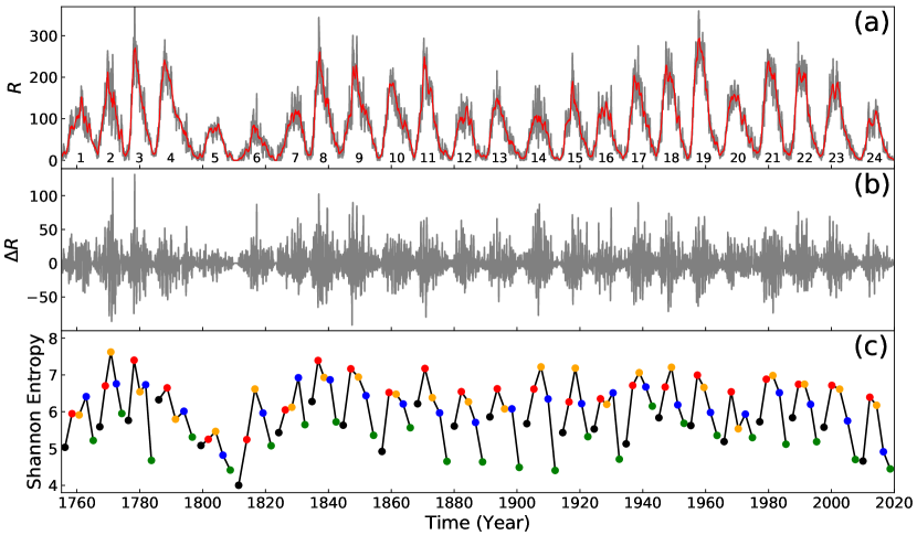
Figure 1: (a) The gray curve shows the monthly SSN for cycles 1$-$24 with the cycle numbers marked, while the red curve presents the running mean value of monthly SSN with a time window of 9 months. (b) The fluctuation of monthly SSN obtained by subtracting the running mean SSN from the monthly SSN. (c) The Shannon entropy is presented with different colors for the 5 phases of each cycle.

The monthly SSN is utilized to obtain the Shannon entropy of solar cycles. The Shannon entropy, also known as information entropy, was proposed by Shannon (1948) to characterize the inherent randomness of a system quantitatively and applied to the study of solar energetic particles (e.g., Laurenza et al., 2012; Qin & Zhao, 2013) as well as solar activity (e.g., Kakad et al., 2015, 2017, 2020; Qin & Wu, 2018) in recent years. The fluctuation of monthly SSN can be treated as a random system, and thereby the Shannon entropy can be obtained from it. Figure 1(a) presents the monthly SSN for cycles 1$-$24 as the gray curve, and the number in the figure indicates the cycle number. We use a time window of 9 months to obtain the running mean value of monthly SSN, which is plotted as the red curve in Figure 1(a). Thus, the fluctuation of monthly SSN, $\Delta R$, can be obtained by subtracting the running mean value from the monthly SSN with

$$\Delta R(i)=R(i)-\frac{1}{w}\sum_{k=i-(w-1)/2}^{i+(w-1)/2}R(k),$$ (1)

where $w$ is the time window. The time sequence of $\Delta R$ is presented in Figure 1(b). It is shown that the variation of $\Delta R$, to some extent, is cyclical, so that we divide each solar cycle to 5 phases evenly to calculate the Shannon entropy of every phase for extracting the characteristics of solar cycles at different phases (e.g., Kakad et al., 2017; Qin & Wu, 2018). The Shannon entropy of each phase, which is computed from the probability density function of $\Delta R$ using the histogram method, can be written as (Wallis, 2006; Kakad et al., 2015, 2017)

$$E=-\sum_{k=1}^{m}p_{k}\text{log}_{2}(p_{k})+\text{log}_{2}(d),$$ (2)

where $E$ is the Shannon entropy, $p_{k}$ is the probability of the $k$th bin of the histogram, $m$ is the number of bins, and $d=3.49\sigma N^{-1/3}$ is the bin width with $\sigma$ and $N$ being the standard deviation and sample size of $\Delta R$, respectively (Scott, 1979). The Shannon entropy is presented with different colors for the 5 phases of each cycle in Figure 1(c). It is shown that the Shannon entropy also shows cyclical characteristics. The values of Shannon entropy are 4.7, 6.4, 6.2, 4.9, and 4.4 for the 5 phases of cycle 24, and that of cycles 1$-$23 can be found in Table 4 of Qin & Wu (2018).

The monthly smoothed SSN is adopted to characterize the solar maximum $S_{m}$ and minimum $S_{0}$ of solar cycles and further to quantify the cycle length $T_{c}$ and ascent time $T_{a}$. The solar maximum is defined as the mathematical maximum of the monthly smoothed SSN in each cycle, while the solar minimum is defined as the mathematical minimum of the monthly smoothed SSN in the period from the preceding solar maximum to the current one. Note that the first occurrence of maximum/minimum value is chosen as the epoch of solar maximum/minimum if the maximum/minimum value occurs more than once in the period. The cycle length are the time interval between the two solar minima at the beginning and end of the solar cycle, while the ascent time are the time interval between the solar minimum at the beginning of the solar cycle and the solar maximum. Cycle 25 started in December 2019, so that the length of cycle 24 is exactly 11 yr and the solar minimum of cycle 25 equals to 1.8.

3 Prediction Model

3.1 TMLP Model

In Qin & Wu (2018), the variation of SSN in a solar cycle is described by the modified logistic function, i.e.,

$$S(x) = r_{0}\left(1-\frac{x^{\alpha}}{x_{m}^{\alpha}}\right)x,$$ (3)

$$x\left(t\right) = x_{m}{\left[1+\left(\frac{x_{m}^{\alpha}}{x_{0}^{\alpha}}-1\right)e^{-\alpha r_{0}t}\right]^{-1/\alpha}},$$ (4)

where $x$ is the cumulative SSN, $t$ is the elapsed time from the solar minimum in units of months, $r_{0}$ is the maximum emergence rate of sunspots, $x_{m}$ is the maximum cumulative SSN or total SSN that can be generated in the cycle, $x_{0}$ is the initial cumulative SSN, and $\alpha$ is the asymmetry of the cycle shape. Hence, the cycle features $S_{m}$, $S_{0}$, $T_{c}$, and $T_{a}$ can be expressed as

$$S_{m} = \frac{\alpha}{1+\alpha}\left(\frac{1}{1+\alpha}\right)^{1/\alpha}r_{0}x_{m},$$ (5)

$$S_{0} = r_{0}\frac{x_{0}}{x_{m}}\frac{x_{m}^{\alpha}-x_{0}^{\alpha}}{x_{m}^{\alpha-1}},$$ (6)

$$T_{c} = \left(12\alpha r_{0}\right)^{-1}\ln{\frac{x_{m}^{\alpha}/x_{0}^{\alpha}-1}{x_{m}^{\alpha}/x_{e}^{\alpha}-1}},$$ (7)

$$T_{a} = \left(12\alpha r_{0}\right)^{-1}\ln{\frac{x_{m}^{\alpha}/x_{0}^{\alpha}-1}{\alpha}},$$ (8)

where $x_{e}$ is the actual total SSN observed in the cycle and can be expressed as $x_{e}=0.9722x_{m}-6.93$. Note that the units of $T_{c}$ and $T_{a}$ are in years. The parameters $r_{0}$ and $\alpha$ were set to 0.2 and 0.224, respectively, for facilitating the construction of SSN prediction model, which was called the TMLP model in Qin & Wu (2018).

The TMLP model can predict the variation of SSN in a solar cycle at the start of the cycle. The key of the prediction made by TMLP is to predict the values of $x_{m}$ and $x_{0}$. The parameter $x_{m}$ of cycle $n$ can be predicted by using the Shannon entropy in the three preceding cycles and the cycle length of the last cycle, i.e.,

$$x_{m}^{\left(n\right)}= - 3509E_{4}^{\left(n-3\right)}+3097E_{2}^{\left(n-2\right)}+4327E_{5}^{\left(n-2\right)}-3190E_{1}^{\left(n-1\right)}$$ (9)

$$+ 3189E_{4}^{\left(n-1\right)}+1397E_{5}^{\left(n-1\right)}-624T_{c}^{\left(n-1\right)}-11862,$$

where the superscript denotes the cycle number, and the subscript of Shannon entropy, $E$, is the phase number of the cycle. The parameter $x_{0}^{\left(n\right)}$ can be obtained approximately by solving Equation (6) with the predicted $x_{m}^{\left(n\right)}$ and the observed solar minimum $S_{0}^{\left(n\right)}$.

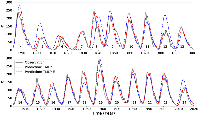
Figure 2: The gray, red dot-dashed, blue dashed lines are the observed monthly smoothed SSN, prediction by TMLP, and prediction by TMLP-E, respectively, for cycles 4$-$24 with the cycle numbers marked.

The observation and prediction for cycles 4$-$24 are presented in Figure 2 with the gray solid and red dot-dashed lines, respectively, and the absolute relative errors of the predicted cycle features are listed in columns 2$-$4 of Table 1. Note that the TMLP model is constructed with the statistical analysis on the observations of cycles 1$-$23 (Qin & Wu, 2018). It is shown that the prediction fits the observation well. The average absolute relative errors of the predicted $S_{m}$, $T_{a}$, and $T_{c}$ are 8.5%, 15.8%, and 9.0% for cycles 4$-$24, respectively. The confidence intervals (CIs) of the predicted $S_{m}$, $T_{a}$, and $T_{c}$ at a 95% significance level are (-22.7%, 18.4%), (-34.6%, 38.8%), and (-23.6%, 17.3%), respectively.

3.2 Extending the Prediction Ability of TMLP Model

Suppose it is currently in cycle $n$, to predict the solar activity of the next cycle, cycle $n+1$, Equation (9) can be rewritten as

$$x_{m}^{\left(n+1\right)}= - 3509E_{4}^{\left(n-2\right)}+3097E_{2}^{\left(n-1\right)}+4327E_{5}^{\left(n-1\right)}-3190E_{1}^{\left(n\right)}$$ (10)

$$+ 3189E_{4}^{\left(n\right)}+1397E_{5}^{\left(n\right)}-624T_{c}^{\left(n\right)}-11862.$$

At the start of cycle $n$, the parameters $E_{1}^{\left(n\right)}$, $E_{4}^{\left(n\right)}$, $E_{5}^{\left(n\right)}$, and $T_{c}^{\left(n\right)}$ are unknown.

$$h(n)=-3190E_{1}^{\left(n\right)}+3189E_{4}^{\left(n\right)}+1397E_{5}^{\left(n\right)}-624T_{c}^{\left(n\right)},$$ (11)

$$\epsilon(n+1)=\frac{\left|h(n)-h(n-1)\right|}{x_{m}^{\left(n+1\right)}}.$$ (12)

Therefore, we replace $E_{i}^{\left(n\right)}$ ($i=1,4,5$) with $E_{i}^{\left(n-1\right)}$, and replace $T_{c}^{\left(n\right)}$ with $T_{c}^{\left(n-1\right)}$ in Equation (10). Then, Equation (10) can be written as

$$x_{m}^{\left(n+1\right)}= - 3509E_{4}^{\left(n-2\right)}-3190E_{1}^{\left(n-1\right)}+3097E_{2}^{\left(n-1\right)}+3189E_{4}^{\left(n-1\right)}$$ (13)

$$+ 5724E_{5}^{\left(n-1\right)}-624T_{c}^{\left(n-1\right)}-11862.$$

$x_{0}^{\left(n+1\right)}$ can be obtained approximately by solving Equation (6) with the predicted $x_{m}^{\left(n+1\right)}$ and the current solar minimum $S_{0}^{\left(n\right)}$. All parameters are available for predicting the variation of SSN in the cycle $n+1$ if the start time of the current cycle $n$ is already known. The new model for predicting the cycle $n+1$ is denoted as TMLP-E.

3.3 Evaluating the Prediction Ability of TMLP-E Model

The prediction results of the TMLP-E for cycles 4$-$24 are presented in Figure 2 with the blue dashed lines, and the absolute relative errors of the predicted cycle features are listed in columns 5$-$7 of Table 1. Although $x_{m}$ and $x_{0}$ are obtained approximately, the prediction result is, however, acceptable for most cycles. The predicted solar maximum deviates from the observation within 20% for more than half of the cycles, while cycles with errors no more than 35% account for 81%.

The prediction errors of solar maximum of cycles 5, 7, 12, and 24 are greater than 35%. Cycles 5, 12, and 24 have a common feature that the solar maximum has a sudden drop (more than 30%) compared to the solar maximum of the preceding cycle. Besides, the Sun entered minima of Gleissberg cycle since cycle 5 and cycle 12, and the Sun might also enter a minimum of Gleissberg cycle since cycle 24. On the other hand, cycle 20, which also has a solar maximum more than 30% less than the preceding one but is not during a minimum of Gleissberg cycle, is predicted with a moderate error (21.5%) for the solar maximum. Therefore, it is supposed that the model can not predict the first solar cycle of the minimum of a Gleissberg cycle accurately. For cycle 7, all the cycle features are predicted with large error, and the prediction is indeed according to the predicted time profile as shown in Figure 2. The prediction is made by mainly using the data of cycle 5 that is during the Dalton minimum. The Shannon entropy of cycle 5 is at an unusually low level because the Dalton minimum has unusually long periods of sunspot inactivity, which might be the reason why the prediction is . Therefore, an prediction may imply a Dalton-like minimum.

The CIs of $S_{m}$, $T_{a}$, and $T_{c}$ are (-41.9%, 33.9%), (-43.1%, 62.5%), and (-28.9%, 22.8%), respectively. It is shown that both the relative error and CI of the predicted $S_{m}$ of TMLP-E are about twice that of TMLP. Besides, both the relative error and CI of the predicted $T_{c}$ of TMLP-E are similar to that of TMLP. In addition, the relative error and CI of the predicted $T_{a}$ of TMLP-E are about 25% and 44% larger than that of TMLP, respectively.

The solar maximum of the TMLP-E result (blue line) is either the largest or the smallest one among the results of observations, TMLP, and TMLP-E in each cycle as shown in Figure 2 except for cycle 17. Therefore, the solar maximum predicted by TMLP-E can be used as either the upper or lower limit to narrow down the CI of the solar maximum predicted by TMLP, although it will slightly increase the prediction error of cycle 17. The solar maxima of the results from observations, TMLP, and TMLP-E for cycles 4$-$24 are listed in columns 2, 3, and 4 of Table 2, respectively. Column 5 gives the CI of the predicted solar maximum of TMLP. The modified CI, listed in Column 6, is obtained by choosing the predicted solar maximum of TMLP-E as either the upper or lower limit if the predicted solar maximum of TMLP-E is within the CI. Column 7 shows whether the prediction of TMLP is improved if we use the modified CI. Note that cycles 5, 7, 12, and 24 are not listed in Table 2. It is shown that almost 82% of CIs predicted by TMLP can be modified, and 93% of the modifications can narrow down the CIs correctly.

4 Results

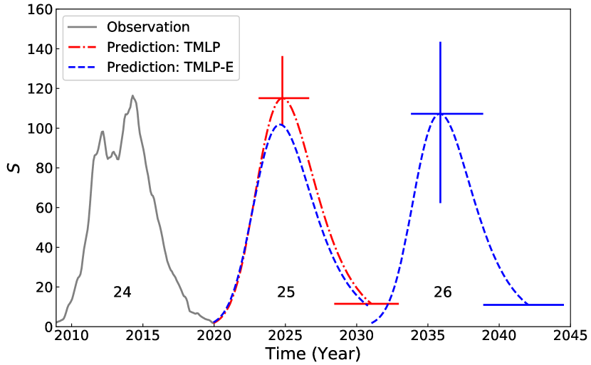
Figure 4: Similar to Figure 2 but for cycles 24$-$26. The vertical error bar shows the CI of the cycle amplitude at a 95% significance level, and the horizontal error bars at the solar maximum and minimum denote the CI of the peak and end time of the cycle, respectively.

In Figure 4, the red dot-dashed line indicates the predicted result of TMLP for cycle 25, and the blue dashed lines indicate the results of TMLP-E for cycles 25 and 26. it is suggested that cycle 24 rather than cycle 25 may be the first cycle of a minimum of Gleissberg cycle in Section 3.3, so that can be predicted with a good accuracy Table 3 gives the values of the predicted cycle features and their CIs. For comparison, the observations of cycle 24 are also presented in the figure and table.

Both models TMLP and TMLP-E could be used for the prediction of cycle 25, here, we use the results from TMLP (red dot-dashed line) as the prediction of cycle 25, and the predicted $S_{m}$, $T_{a}$, and $T_{c}$ are 115.1, 4.84 yr, and 11.06 yr, respectively. In addition, the CIs of the predicted $S_{m}$, $T_{a}$, and $T_{c}$ are (89.0, 136.3), (3.17 yr, 6.72 yr), and (8.45 yr, 12.98 yr), respectively. On the other hand, if we use model TMLP-E to predict cycle 25, the $S_{m}$ is obtained as 101.8, which is less than the $S_{m}$ predicted by TMLP, so that the CI of the $S_{m}$ can be modified to (101.8, 136.3).

Model TMLP-E can be used to predict cycle 26 shown in Figure 4, and the predicted $S_{m}$, $T_{a}$, and $T_{c}$ are 107.3, 4.80 yr, and 10.97 yr, respectively. Furthermore, the CIs of the $S_{m}$, $T_{a}$, and $T_{c}$ are (62.3, 143.6), (2.74 yr, 7.81 yr), and (7.81 yr, 13.47 yr), respectively. It is shown that the predictions of cycles 25 and 26 are similar to the observation of cycle 24.

5 CONCLUSIONS AND DISCUSSION

In this paper, we use the TMLP and TMLP-E models to predict the SSNs of cycles 25 and 26. The TMLP model, which is proposed by Qin & Wu (2018), has two parameters, namely, the maximum cumulative SSN $x_{m}$ and the initial cumulative SSN $x_{0}$. The parameter $x_{m}$ of cycle $n$ can be expressed as the linear combination of the Shannon entropy of the three preceding cycles and the length of the last cycle, i.e., Equation (9). The other parameter $x_{0}$ can be estimated by solving Equation (6) with the predicted $x_{m}$ and observed $S_{0}$ of cycle $n$. Therefore, the variation of SSNs in cycle $n$ can be predicted by the TMLP model if the start time of cycle $n$ is already known. To predict the variation of SSNs in cycle $n+1$, we extend the TMLP to TMLP-E by assuming that the behavior of cycle $n$ would be similar to that of cycle $n-1$, i.e., one may replace the Shannon entropy and cycle length of cycle $n$ with that of cycle $n-1$, and replace the solar minimum of cycle $n+1$ with that of cycle $n$. With this assumption, $x_{m}$ of cycle $n+1$ can be predicted with the Shannon entropy of cycles $n-1$ and $n-2$ and the length of cycle $n-1$, and $x_{0}$ can be estimated with the predicted $x_{m}$ and the solar minimum of cycle $n$. Therefore, the variation of SSN in cycle $n+1$ can be predicted by the TMLP-E model when the start time of cycle $n$ has been determined. All in all, the TMLP and TMLP-E models can predict monthly smoothed SSNs nearly one and two cycles in advance, respectively.

The prediction ability of TMLP-E is evaluated with the prediction accuracy of cycles 4$-$24. Note that, cycles 5, 7, 12, and 24 are excluded if we are not going to predict the first cycle of the minimum of a Gleissberg cycle, and if we do not consider the predictions. The average absolute relative errors of the solar maximum, ascent time, and cycle length predicted by TMLP-E are 16.8%, 19.7%, and 10.3%, respectively. CIs of the predicted solar maximum, ascent time, and cycle length are (-41.9%, 33.9%), (-43.1%, 62.5%), and (-28.9%, 22.8%), respectively, at a 95% significance level. Besides, the solar maximum predicted by TMLP-E can be used to narrow down the CI of the solar maximum predicted by TMLP for most cycles.

The solar maximum of cycle 25 predicted by TMLP is 115.1, and the CI at a 95% significance level is (89.0, 136.3), which can be further modified to (101.8, 136.3) by the predicted solar maximum of TMLP-E. The solar maximum would occur in October 2024 (95% CI is from February 2023 to September 2026), and cycle 25 would end in January 2031 (95% CI is from May 2028 to December 2032). The solar maximum of cycle 26 predicted by TMLP-E is 107.3 (95% CI is 62.3$-$143.6). If the end time of cycle 25 predicted by the TMLP is chosen as the start time of cycle 26, the solar maximum is expected to appear in November 2035 (95% CI is from October 2033 to November 2038), and cycle 26 would end in January 2041 (95% CI is from November 2038 to July 2044). The solar maxima of cycles 25 and 26 are predicted to be at a low level and similar to that of cycle 24, which is about 40% greater than the solar maximum of cycle 5 or cycle 6. We therefore suggest that the declining trend of solar activity will break and cycles 24$-$26 are at a minimum of Gleissberg cycle rather than a Dalton-like minimum.

The Solar Cycle Prediction Panel experts released a forecast for cycle 25 in 2019 (see https://www.weather.gov/news/190504-sun-activity-in-solar-cycle), and the solar maximum was expected to be in the range between 95 and 130 and would peak during the time interval 2023$-$2026. the prediction results for cycle 25 in this work are very similar to that reported by the Solar Cycle Prediction Panel experts

Several research inferred that the strong suppression of some parameters such as the occurrence rate of flares in cycle 23 compared to cycle 22 may be the earlier sign of the sudden drop of solar activity from cycle 23 to 24 (Petrovay, 2020, and references therein). In this work, TMLP-E can not predict the first solar cycle of the minimum of Gleissberg cycle accurately about two cycles in advance while TMLP can forecast it well about one cycles in advance. Therefore, we suggest that the preceding cycle is important for predicting the sudden drop of solar activity or the start of a new Gleissberg cycle.

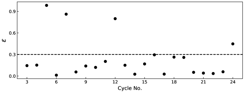
Figure 3: The absolute relative error $\epsilon$ given by Equation (12) for cycles 3$-$24.

Table 1: Absolute relative errors of predicted cycle features for cycles 4$-$24.

	TMLP				TMLP-E
Cycle No.	$\delta S_{m}/S_{m}$	$\delta T_{a}/T_{a}$	$\delta T_{c}/T_{c}$		$\delta S_{m}/S_{m}$	$\delta T_{a}/T_{a}$	$\delta T_{c}/T_{c}$
4	2.0%	16.3%	22.1%		18.4%	24.4%	19.6%
5	1.1%	41.5%	16.4%		109.1%	45.3%	14.4%
6	10.3%	5.4%	8.8%		11.4%	34.2%	22.4%
7	3.9%	10.8%	14.0%		96.3%	36.8%	46.6%
8	5.5%	23.7%	10.9%		10.2%	87.4%	32.6%
9	2.9%	16.6%	16.4%		11.7%	9.2%	13.2%
10	11.1%	7.8%	1.9%		23.6%	7.0%	7.0%
11	8.4%	23.2%	8.3%		24.9%	28.6%	7.6%
12	1.0%	10.6%	4.6%		77.3%	15.5%	4.0%
13	13.2%	3.9%	13.2%		27.6%	14.3%	10.9%
14	0.5%	4.4%	9.3%		2.3%	4.9%	12.5%
15	21.9%	16.6%	10.9%		35.0%	5.5%	5.2%
16	15.9%	15.5%	2.3%		13.8%	2.2%	6.7%
17	11.9%	23.1%	4.4%		9.4%	15.2%	1.9%
18	8.1%	22.9%	3.5%		33.2%	32.4%	4.9%
19	18.9%	18.7%	7.1%		3.8%	8.4%	4.1%
20	15.3%	5.7%	9.5%		21.5%	11.1%	3.3%
21	10.3%	1.3%	1.4%		14.2%	4.6%	0.5%
22	5.1%	25.3%	8.6%		8.3%	18.4%	6.2%
23	9.3%	25.9%	15.8%		15.6%	27.5%	16.3%
24	1.4%	11.0%	0.2%		41.3%	25.8%	5.6%
avg.	8.5%	15.7%	9.0%		29.0%	21.8%	11.7%
std.	6.2%	9.8%	5.8%		29.6%	19.4%	11.2%

Table 2: Modification of CI of the solar maximum predicted by TMLP.

Cycle No.	$S_{m}^{\text{obs}}$	$S_{m}^{\text{TMLP}}$	$S_{m}^{\text{TMLP-E}}$	CI	Modified CI	Improved
4	235.3	240.0	278.5	(185.6, 284.1)	(185.6, 278.5)	Yes
6	81.2	89.6	90.4	(69.3, 106.1)	(69.3, 90.4)	Yes
8	244.9	231.3	220.0	(178.9, 273.8)	(220.0, 273.8)	Yes
9	219.9	213.5	245.7	(165.1, 252.7)	(165.1, 245.7)	Yes
10	186.2	206.9	230.1	(160.0, 244.9)	(160.0, 230.1)	Yes
11	234.0	214.3	175.7	(165.7, 253.6)	(175.7, 253.6)	Yes
13	146.5	127.2	106.0	(98.3, 150.5)	(106.0, 150.5)	Yes
14	107.1	106.6	109.6	(82.4, 126.1)	(82.4, 109.6)	Yes
15	175.7	137.3	114.2	(106.2, 162.5)	(114.2, 162.5)	Yes
16	130.2	150.9	112.2	(116.7, 178.6)	—	—
17	198.6	175.0	180.0	(135.3, 207.2)	(135.3, 180.0)	No
18	218.7	200.9	146.0	(155.3, 237.8)	—	—
19	285.0	231.0	295.7	(178.7, 273.5)	—	—
20	156.6	180.6	190.3	(139.6, 213.8)	(139.6, 190.3)	Yes
21	232.9	208.8	199.9	(161.5, 247.2)	(199.9, 247.2)	Yes
22	212.5	201.7	194.8	(156.0, 238.7)	(194.8, 238.7)	Yes
23	180.3	197.2	208.3	(152.5, 233.4)	(152.5, 208.3)	Yes

Table 3: Predicted cycle features of cycles 25$-$26.

Cycle No.	Model	$S_{m}$	CI${}_{S_{m}}$	Modified CI${}_{S_{m}}$	$T_{a}$	CI${}_{T_{a}}$	$T_{cy}$	CI${}_{T_{cy}}$
24	Observation	116.4	—	—	5.33	—	11.00	—
25	TMLP	115.1	(89.0, 136.3)	(101.8, 136.3)	4.84	(3.17, 6.72)	11.06	(8.45, 12.98)
	TMLP-E	101.8	(59.2, 136.3)	—	4.66	(2.65, 7.58)	10.79	(7.68, 13.25)
26	TMLP-E	107.3	(62.3, 143.6)	—	4.80	(2.74, 7.81)	10.97	(7.81, 13.47)

References

- Abdusamatov (2007) Abdusamatov, K. I. 2007, KPCB, 23, 97
- Balogh et al. (2014) Balogh, A., Hudson, H. S., Petrovay, K., & von Steiger, R. 2014, Space Sci. Rev., 186, 1
- Bhowmik & Nandy (2018) Bhowmik, P., & Nandy, D. 2018, NatCo, 9, 5209
- Charvátová (2009) Charvátová, I. 2009, New A, 14, 25
- Chen et al. (2021) Chen, Y.-Q., Zheng, S., Xiao, Y.-S., et al. 2021, Atmos, 12, 1176
- Choudhuri et al. (2007) Choudhuri, A. R., Chatterjee,P., & Jiang, J. 2007, Phys. Rev. Lett., 98, 131103
- Clette et al. (2015) Clette, F., Cliver, E. W., Lefèvre, L., Svalgaard, L., & Vaquero, J. M. 2015, SpWea, 13, 529
- Clette & Lefèvre (2016) Clette, F., & Lefèvre, L. 2016, Sol. Phys., 291, 2629
- Covas et al. (2019) Covas, E., Peixinho, N., & Fernandes, J. 2019, Sol. Phys., 294, 24
- Dikpati et al. (2006) Dikpati, M., Toma, G. De, & Gilman, P. A. 2006, Geophys. Res. Lett., 33, L05102
- Du (2020) Du, Z. L. 2020, Ap&SS, 365, 104
- Eddy (1976) Eddy, J. A. 1976, Science, 192, 1189
- Gleissberg (1939) Gleissberg, W. 1939, Obs, 62, 158
- Gonçalves et al. (2020) Gonçalves, Í. G., Echer, E., & Frigo, E. 2020, AdSpR, 65, 677
- Han & Yin (2019) Han, Y. B., & Yin, Z. Q. 2019, Sol. Phys., 294, 107
- Hathaway (2015) Hathaway, D. H. 2015, LRSP, 12, 4
- Hiremath (2008) Hiremath, K. M. 2008, Ap&SS, 314, 45
- Hunter (2007) Hunter, J. D. 2007, CSE, 9, 90
- Javaraiah (2017) Javaraiah, J. 2017, Sol. Phys., 292, 172
- Jiang et al. (2018) Jiang, J., Wang, J.-X., Jiao, Q.-R., & Cao, J.-B. 2018, ApJ, 863, 159
- Kakad et al. (2015) Kakad, B., Kakad, A., & Ramesh, D. S. 2015, JSWSC, 5, A29
- Kakad et al. (2017) Kakad, B., Kakad, A., & Ramesh, D. S. 2017, Sol. Phys., 292, 95
- Kakad et al. (2020) Kakad, B., Kumar, R., & Kakad, A. 2020, Sol. Phys., 295, 88
- Karak & Nandy (2012) Karak, B. B., & Nandy, D. 2012, ApJ, 761, L13
- Kitiashvili (2020) Kitiashvili, I. N. 2020, ApJ, 890, 36
- Labonville et al. (2019) Labonville, F., Charbonneau, P., & Lemerle, A. 2019, Sol. Phys., 294, 82
- Lanzerotti (2017) Lanzerotti, L. J. 2017, Space Sci. Rev., 212, 1253
- Laurenza et al. (2012) Laurenza, M., Consolini, G., Storini, M., & Damiani, A. 2012, ASTRA, 8, 19
- Lee (2020) Lee, T. 2020, Sol. Phys., 295, 82
- Li et al. (2018) Li, F. Y., Kong, D. F., Xie, J. L., Xiang, N. B., & Xu, J. C. 2018, JASTP, 181, 110
- Lin et al. (2019) Lin, G. H., Wang, X. F., Liu, S., et al. 2019, Sol. Phys., 294, 79
- Macario-Rojas et al. (2018) Macario-Rojas, A., Smith, K. L., & Roberts, P. C. E. 2018, MNRAS, 479, 3791
- Mertens et al. (2018) Mertens, C. J., Slaba, T. C., & Hu, S. 2018, SpWea, 16, 1291
- Muñoz-Jaramillo et al. (2012) Muñoz-Jaramillo, A., Sheeley, N. R., Zhang, J., & DeLuca, E. E. 2012, ApJ, 753, 146
- Nandy (2021) Nandy, D. 2021, Sol. Phys., 296, 54
- Okoh et al. (2018) Okoh, D. I., Seemala, G. K., Rabiu, A. B., et al. 2018, SpWea, 16, 1424
- Pesnell (2016) Pesnell, W. D. 2016, SpWea, 14, 10
- Pesnell & Schatten (2018) Pesnell, W. D., & Schatten, K. H. 2018, Sol. Phys., 293, 112
- Petrovay (2020) Petrovay, K. 2020, LRSP, 17, 2
- Qin & Wu (2018) Qin, G., & Wu, S.-S. 2018, ApJ, 869, 48
- Qin & Zhao (2013) Qin, G., & Zhao, L.-L. 2013, arxiv:1312.2296
- Sarp et al. (2018) Sarp, V., Kilcik, A., Yurchyshyn, V., Rozelot, J. P., & Ozguc, A. 2018, MNRAS, 481, 2981
- Scott (1979) Scott, D. W. 1979, Biometrika, 66, 605
- Shannon (1948) Shannon, C. E. 1948, BSTJ, 27, 379
- Shen & Qin (2018) Shen, Z.-N., & Qin, G. 2018, ApJ, 854, 137
- Singh & Bhargawa (2019) Singh, A. K., & Bhargawa, A. 2019, Ap&SS, 364, 12
- Singh et al. (2019) Singh, P. R., Tiwari, C. M., Saxena, A. K., & Agrawal, S. L. 2019, Phys. Scr, 94, 105005
- Upton & Hathaway (2018) Upton, L. A., & Hathaway, D. H. 2018, GeoRL, 45, 8091
- Wallis (2006) Wallis, K. F. 2006, MPRA Paper, University Library of Munich, Germany
- Wu & Qin (2018) Wu, S.-S., & Qin, G. 2018, JGRA, 123, 76
- Yeates et al. (2008) Yeates, A. R., Nandy, D., & Mackay, D. H. 2008, ApJ, 673, 544