Fairness Through Regularization
for Learning to Rank

Abstract

Given the abundance of applications of ranking in recent years, addressing fairness concerns around automated ranking systems becomes necessary for increasing the trust among end-users. Previous work on fair ranking has mostly focused on application-specific fairness notions, often tailored to online advertising, and it rarely considers learning as part of the process. In this work, we show how to transfer numerous fairness notions from binary classification to a learning to rank setting. Our formalism allows us to design methods for incorporating fairness objectives with provable generalization guarantees. An extensive experimental evaluation shows that our method can improve ranking fairness substantially with no or only little loss of model quality.

1 Introduction

Ranking problems are abundant in many contemporary subfields of machine learning and artificial intelligence, including web search, question answering, candidate/reviewer allocation, recommender systems and bid phrase suggestions [43]. Decisions taken by such ranking systems affect our everyday life and this naturally leads to concerns about the fairness of ranking algorithms.

Indeed, ranking systems are typically designed to maximize utility and return the results most likely correct for each query [53]. This can have potentially harmful down-stream effects. For example, in 2015 Google became the target of heavy criticism after news reports that when searching for ”CEO” in Google’s image search, the first image of a women appeared only in the twelfth row, requiring two page scrolls to reach, and it actually did not show a real person but a Barbie doll [42]. Similar problems still exist in other ranking applications, such as product recommendations or online dating.

Potentially biased or otherwise undesirable results are particularly problematic in the learning to rank (LTR) setting [41, 45], where a machine learning model is trained to predict the relevances of the items for any query at test time. Training data for these systems is typically obtained from users interacting with another ranking system. Therefore, a biased selection of items can lead to disadvantageous winner-takes-it-all and rich-get-richer dynamics [59, 61].

A number of ranking-related fairness notions were proposed to make ranking systems more fair [10, 56, 75]. However, these were tailored to specific applications, such as online advertising. Some are also not well suited to the LTR situation, because their associated algorithms work by directly manipulating the order of returned items for a given query. In contrast, in the LTR setting one would hope that the system learns to be fair, such that a manipulation of the predicted relevance scores or the order of items are not necessary. This latter aspect brings up the problem of generalization for fairness: a ranking method could appear fair on the training data but turn out unfair at prediction time.

In this paper, we address these challenges and develop fairness-aware algorithms for LTR that provably generalize. To this end, we exploit connections between ranking and classification. Indeed, in contrast to fair learning in information retrieval, fair classification is a widely studied area where both the algorithmic and learning theoretic challenges of learning fair models are rather well understood [5, 23, 68]. Importantly, many different notions of fairness have been proposed, which describe different properties that are desirable in various applications [44].

We provide a formalism for translating such well-established and well-understood fairness notions from classification to ranking by phrasing the LTR problem as a binary classification problem for every query-item pair. We exemplify our approach on three fairness notions that emerge naturally in the ranking setting and correspond to popular concepts in classification: demographic parity, equalized odds, and equality of opportunity. We then formulate corresponding fairness regularization terms, which can be incorporated with minor overhead into many standard LTR algorithms.

Besides its flexibility, another advantage of our approach is that it makes the task of fair LTR readily amendable to a learning-theoretic analysis. Specifically, we show generalization bounds for the three considered fairness notions, using a chromatic concentration bound for sums of dependent random variables [31] to overcome the challenge that training samples for the same query are not independent.

Finally, we demonstrate the practical usefulness of our method for training fair models. Experiments on two ranking datasets confirm that training with our regularizers indeed yields models with greatly improved fairness at prediction time, often with little to no reduction of ranking quality. In contrast, prior fair ranking methods are unable to consistently improve our fairness notions.

2 Related work

Fairness in classification.  Algorithmic fairness is well explored in the context of binary classification, see [5] for a detailed introduction. In this work we show how to extend three popular group fairness notions – demographic parity, equalized odds and equality of opportunity [30] – to the ranking setting. In principle, our formalism is applicable to other group fairness notions, as well as individual [25] and causal [40] fairness notions. We defer the exploration of these to future work. On the methodological level, we opt for a highly adaptive and scalable regularization approach, inspired by successful regularization methods for fair classification [34, 36, 73]. More generally any other fair classification technique, e.g. [4, 22, 38, 52, 60, 77], may be applicable to our framework.

Fairness in ranking.  Fairness in ranking has so far received less attention than fairness in classification. For an overview of recent techniques, see [18]. Most existing works concentrate on application-specific (single-purpose) fairness notions. One popular concept is fairness of exposure [10, 28, 46, 54, 56, 57, 70, 74]. It states that exposure/attention received by a group of items or an individual item should be proportional to its utility. Other works aim at ensuring sufficient representation of items from different groups in the top-$k$ positions of a ranking [19, 20, 27, 71, 75]. Besides group fairness also fair treatment of individuals has been studied in the context of ranking [13, 72].

Among papers considering broader notions of fairness in ranking, [3] designs learning algorithms that can work with any fairness oracle. The framework however is limited to linear classifiers and the authors do not propose specific fairness notions. [55] introduces a number of fair ranking definitions and draws parallels to equalized odds and demographic parity from fair classification. However, it does not provide a formal framework from studying the correspondence between the two setups, and does not study how to optimize these measures in a learning to rank context. Moreover, its fairness measures concern fair rankings for a fixed query, which also holds for the causal fairness notion in [69]. In contrast, our notion of ranking fairness is amortized across queries, similarly to [10].

Another related line of work is the one of pairwise fairness [8, 39, 47]. These works also describe ranking as a classification task in order to define fairness. However, the considered task is the proxy commonly employed by pairwise ranking methods, namely predicting which one of two items is more relevant than the other for a given query. In contrast, we define fairness in direct relation to the downstream task of deciding whether to return an item as relevant for a query or not. [33, 64] introduce fairness notions for bipartite ranking. These are also based on pairwise comparisons between points, but aim at learning fair continuous risks scores.

Overall, the main difference of our work to previous ones on ranking fairness is that we do not introduce a new fairness notion or algorithm. Instead, the formalism we introduce allows transferring existing fairness notions from classification to ranking. A second distinction is that only a minority of prior works considers fairness in the context of learning, and those who do usually propose new training techniques. Instead, the fairness regularizers we introduce can be combined with any existing training procedure that can be formulated as learning a score function by minimizing a cost function. Finally, no prior works provides generalization guarantees for fair ranking as we do.

Fairness in recommender systems.  For recommender systems, fairness can be studied with respect to the consumers/users (known as C-fairness) or with respect to the providers/items (known as P-fairness) [14]. [58, 61] consider calibration and bias disparity within recommender systems with respect to recommended items. In [15, 26, 78, 21, 50] various hybrid approaching for achieving both C-fairness and P-fairness are presented. In contrast to our paper, these works are specific to collaborative filtering or tensor-based algorithms and do not carry over to approaches based on supervised learning.

A concept from recommender systems related to demographic parity fairness is that of neutrality [35], in which one aims to provide recommendations that are independent of a certain viewpoint. In particular, [35, 37] apply a neutrality enhancing regularizer to a recommender system model. The focus of these works, however, lies on dealing with filter bubble problems and no formal links to classification or fairness are made.

Diversity in ranking.  Another related topic is the one of diversifying the output set of ranking system, see,e.g., [51]. However, diversifying rankings generally has the goal of improving the user experience, not a fair treatment of items. A discussion on the relationship between fairness and ranking diversity can be found in [56].

3 Preliminaries

In this section we introduce some background information on the learning to rank (LTR) task. A thorough introduction can be found, e.g., in [41, 45].

Learning to rank.  Let $\mathcal{Q}$ be a set of possible queries to a ranking system, and let $\mathcal{D}$ be a set of items (historically documents) that are meant to be ranked according to their relevance for any query. Typically, we think of the query set as practically infinite, e.g. natural language phrases, whereas the item set is finite and fixed, e.g. a database of products or customers. These are not fundamental constraints, though, and extensions are possible, e.g. items appearing or disappearing over time.

A dataset in the LTR setting typically has the form $S=\{(q_{i},d^{i}_{j},r_{j}^{i})\}_{i\in[N],j\in[m_{i}]}$, i.e. for each of $N$ queries, $q_{1},\ldots,q_{N}\in\mathcal{Q}$, a subset of the items $D_{q_{i}}=\{d^{i}_{1},d^{i}_{2},\ldots,d^{i}_{m_{i}}\}\subset\mathcal{D}$ are annotated with binary labels $r_{j}^{i}=r(q_{i},d^{i}_{j})\in\{0,1\}$ that indicate if item $d^{i}_{j}$ is relevant to query $q_{i}$ or not. In most real-world scenarios, $m_{i}$ will be much smaller than $|\mathcal{D}|$, since it is typically impractical to determine the relevance of every item for a query.

The goal of learning to rank is to use a given training set to learn a ranking procedure that, for any future query, can return a set of items as well as their order. That is, the learner has to construct a subset selection function,

$$R:\mathcal{Q}\to\mathfrak{P}(\mathcal{D}),$$ (1)

where $\mathfrak{P}$ denotes the powerset operation, as well as an ordering of the predicted item set. In practice, both steps are typically combined by learning a score function, $s:\mathcal{Q}\times\mathcal{D}\to\mathbb{R}$. For any fixed $q$, $s(q,\cdot)$ induces a total ordering of $\mathcal{D}$, and the set of predicted items is obtained by thresholding or top-$k$ prediction. The function $s$ is usually learned by minimizing a loss function on the quality of the resulting ranking on the train data. Classic examples of this construction are SVMRank [32] or WSABIE [65]. Most other pointwise, pairwise and listwise methods can also be phrased in the above way, with differences mainly in how the loss is defined and how the score function is learned numerically [41].

Evaluation measures.  Many measures exist for evaluating the quality of a ranking system. Arguably the simplest is to measure the fraction of correctly predicted relevant items.

Definition 1.

Let $S$ be a test set in the format introduced above. For any query $q_{i}$, let $d^{i}_{1},d^{i}_{2},\dots$ be a ranking of the items in $\mathcal{D}_{q_{i}}$ with associated ground-truth values $r(q_{i},d^{i}_{j})$. Then, for any $k\in\mathbb{N}\setminus\{0\}$, the precision at $k$ is defined as $\operatorname{P@k}=\frac{1}{N}\sum_{i=1}^{N}P@k(q_{i})$ with

$$\operatorname{P@k}(q_{i})=\frac{1}{k}\sum_{j=1}^{k}r(q_{i},d^{i}_{j}).$$ (2)

For any $k$, the $\operatorname{P@k}$ value reflects only which items appear in the top-$k$ list, but not their ordering. Furthermore, $\operatorname{P@k}$ is automatically small for datasets in which queries have only few relevant documents. To mitigate these shortcomings, one can add position-dependent weights and normalize by the score of a best-possible ranking.

Definition 2.

In the same setting as for Definition 1, the normalized discounted cumulative gain at $k$ is defined as $\operatorname{NDCG}\!\mathit{@k}=\frac{1}{N}\sum_{i=1}^{N}\operatorname{NDCG}\!\mathit{@k}(q_{i})$ for

$$\operatorname{NDCG}\!\mathit{@k}(q_{i})=\Big{(}\sum_{j=1}^{k}\frac{r(q_{i},d^{i}_{j})}{\log_{2}(j+1)}\Big{)}\left.\middle/\right.\Big{(}\sum_{j=1}^{\min(k,K_{i})}\frac{1}{\log_{2}(j+1)}\Big{)},$$ (3)

where $K_{i}=|\{d\in\mathcal{D}_{q_{i}}\ :\ r(q_{i},d)=1\}|$ is the number of relevant items for query $q_{i}$. Queries with no relevant items are excluded from the average, as the measure is not well-defined for these.

4 Fairness in Learning-to-Rank

We now introduce our framework for group fairness in ranking. The main step is to exploit a correspondence between ranking and multi-label learning, a view that has previously been employed for practical tasks, e.g., in extreme classification [7], but not –to our knowledge– to make LTR benefit from prior work on classification fairness.

Specifically, we study how a set of relevant items for any query can be selected in a fairly. Analogously to the discussion in Section 3, this originally means learning a subset selection function $R:\mathcal{Q}\to\mathfrak{P}(\mathcal{D})$, where $R(q)$ is the predicted set of selected items for a query $q$. The objects for which we want to impose fairness, the items, occur as outputs of the learned functions. This makes it hard to leverage fairness notions from classification, where fairness is defined with respect to the inputs.

We advocate an orthogonal viewpoint: for any fixed query $q$, we treat the items not as elements of the predictor’s output, but as the inputs to a query-dependent classifier: $f_{q}:\mathcal{D}\to\{0,1\}$, where $f_{q}(d)=1$, if item $d$ is should be returned for query $q$, and $f_{q}(d)=0$ otherwise. As the query is a priori unknown, this means one ultimately has to find an item selection function

$$f:\mathcal{Q}\times\mathcal{D}\to\{0,1\}.$$ (4)

While, of course, both views are equivalent, the latter one allows us to readily integrate notions of classification fairness into the LTR paradigm. Here we focus on the inclusion of group fairness, and leave the derivation of individual fairness [25] or counterfactual fairness [40] to future work.

Note that even though the item selection function $f(q,d)$ and the relevance label $r(q,d)$ have the same signature, their roles are different. $r$ specifies if an item is relevant for a query or not. $f$ indicates if the item should be returned as a result. These concepts differ when other aspects besides relevance are meant to influence the ranking, such as an upper bound on how many items can be retrieved per query or fairness and diversity considerations.

4.1 Group fairness in learning to rank

Notions of group fairness in classification are typically based on an underlying probabilistic framework that allows statements about (conditional) independence relations [5]. The same is true in the ranking situation, where we assume $\mathbb{P}\in\mathcal{P}(\mathcal{Q}\times\mathcal{D}\times\{0,1\})$ to be an unknown but fixed distribution over query/document/relevance triplets. In the rest of our work, all statements about probabilities of events, denoted by $\Pr$, will be with respect to $\mathbb{P}(q,d,r(q,d))$. Note that $\mathbb{P}$ characterizes only the marginal distribution of observing individual data points. It does not further specify how sets of many points, e.g. a training dataset, would be sampled. In particular, as we will discuss later, datasets for ranking tasks are typically not sampled i.i.d. from $\mathbb{P}$, but exhibit strong statistical dependencies.

Analogously to the situation of classification, we assume that any item $d\in\mathcal{D}$ has a protected attribute, $A(d)$, which denotes the group membership for which fairness should be ensured. For example, $A(d)$ can correspond to gender, when the retrieved items are images of people, or to the country of origin of an Amazon product. In this work, we assume binary-valued protected attributes, but this is only for simplicity of presentation, not a fundamental limitation of our framework.

A plausible notion of fairness in the context of ranking is: For any relevant item the probability of being included in the ranker’s output should be independent of its protected attribute. This intuition is easy to formulate in our formalism, resulting a direct analog of the equality of opportunity principle from fair classification [30].

Definition 3 (Equality of opportunity for LTR).

An item selection function $f:\mathcal{Q}\times\mathcal{D}\to\{0,1\}$ fulfills the equality of opportunity condition, if

$$\begin{split}&\Pr(f(q,d)=1|A(d)=0,r(q,d)=1)=\Pr(f(q,d)=1|A(d)=1,r(q,d)=1).\end{split}$$ (5)

where $A(d)$ denotes the protected attribute of a document $d$.

The above definition provides a formal criterion of what it means for a ranking system to be fair. In practice, a ranker will rarely achieve perfect fairness. Therefore, we also introduce a quantitative version of Definition 3 in the form of a fairness deviation measure [67, 68] that reports a ranking procedure’s amount of unfairness (or lack of fairness) by means of its mean difference score [16].

Definition 4.

The equality of opportunity (EOp) violation of any item selection function, $f:\mathcal{Q}\times\mathcal{D}\to\{0,1\}$, is

$$\begin{split}\Gamma^{\textrm{EOp}}(f)&=\Big{|}\Pr(f(q,d)\!=\!1|A(d)\!=\!0,r(q,d)\!=\!1)-\Pr(f(q,d)\!=\!1|A(d)\!=\!1,r(q,d)\!=\!1)\Big{|}.\end{split}$$

Clearly, $f$, is fair in the sense of Definition 3 if and only if it fulfills $\Gamma^{\textrm{EOp}}(f)=0$.

Other fairness measures.  As discussed extensively in the literature, different notions of fairness are appropriate under different circumstances. For example, to check the equality of opportunity condition one needs to know which items are relevant for a query, and this can be problematic, e.g., if the available data itself exhibits a bias in this respect.

A major advantage of our formalism compared to prior fair ranking methods is that it is not partial to a specific fairness measure. Besides equality of opportunity, many other notions of group fairness can be expressed by simply translating the corresponding expressions from classification.

For example, one can avoid the problem of a data bias by simply demanding: The probability of any item to be selected should be independent of its protected attribute (disregarding its relevance to the query). In our formalism, this condition is a direct analog of demographic parity [17].

Definition 5 (Demographic Parity for LTR).

An item selection function $f:\mathcal{Q}\times\mathcal{D}\to\{0,1\}$ fulfills the demographic parity condition, if

$$\Pr(f(q,d)\!=\!1|A(d)\!=\!0) \!=\!\Pr(f(q,d)\!=\!1|A(d)\!=\!1).$$ (6)

As associated quantitative measure we define the demographic parity (DP) violation of $f$ as

$$\begin{split}\Gamma^{\textrm{DP}}(f)&=\Big{|}\Pr(f(q,d)=1|A(d)=0)-\Pr(f(q,d)=1|A(d)=1)\Big{|}.\end{split}$$

Another meaningful notion of fairness in ranking is: The probability of any item to be selected should be independent of its protected attribute, individually for all relevant and for all irrelevant items. This condition yields the ranking analog of the equality odds criterion  [30].

Definition 6 (Equalized Odds for LTR).

An item selection function $f:\mathcal{Q}\times\mathcal{D}\to\{0,1\}$ fulfills the equalized odds condition, if for all $r\in\{0,1\}$:

$$\begin{split}&\Pr(f(q,d)=1|A(d)=0,r(q,d)=r)=\Pr(f(q,d)=1|A(d)=1,r(q,d)=r)\end{split}$$ (7)

The equalized odds (EOd) violation of $f$ is

$$\Gamma^{\textrm{EOd}}(f) =\frac{1}{2}\!\!\!\sum_{r\in\{0,1\}}\!\!\!\Big{|}\Pr(f(q,d)\!=\!1|A(d)\!=\!0,r(q,d)\!=\!r)-\Pr(f(q,d)\!=\!1|A(d)\!=\!1,r(q,d)\!=\!r)\Big{|}.$$

4.2 Training fair rankers

The above definitions do not only allow measuring the fairness of a fixed ranking system, but any of them can also be used to enforce the fairness of a LTR system during the training phase. For this, we create empirical variants of the fairness violation measures and add them as a regularizer during the training step  [2, 34]. For this construction to make sense, we have to answer two questions: Can we solve the resulting optimization efficiently? and Does the inclusion of a regularizer generalize, i.e. ensure fairness also on future predictions? In rest of this section, we will answer the first question. The second question we will address in Section 4.3.

To allow for gradient-based optimization, we parametrize the binary-valued item selection function in a differentiable way using a real-valued score function $s:\mathcal{Q}\times\mathcal{D}\to[0,1]$, similar as introduced in Section 3. Our inspiration, however, comes from the classification setting, such as logistic regression, and we assume that $s$ is not arbitrary real-valued, but that it parameterizes the probability that $d$ is selected for $q$, i.e. $s(q,d)=\Pr(f(q,d)=1)$.

Empirical fairness measures.  For a given training set, $S$, in the format discussed in Section 3, we obtain empirical estimates of the previously introduced fairness violation measures. For any $a\in\{0,1\}$, $r\in\{0,1\}$, denote by $S_{a}$ the subset of data points $(q,d,r(q,d))$ in $S$ with $A(d)=a$, and by $S_{a,r}$ the subset of data points in $S$ with $A(d)=a$ and $r(q,d)=r$.

Definition 7 (Empirical fairness violation measures).

For any function $s:\mathcal{Q}\times\mathcal{D}\to[0,1]$, its empirical equality of opportunity violation on a dataset $S$ is

$$\begin{split}{\Gamma^{\textrm{EOp}}}(s;S)&=\Big{|}\frac{1}{|S_{0,1}|}\!\!\sum_{(q,d)\in S_{0,1}}\!\!\!\!\!\!s(q,d)-\frac{1}{|S_{1,1}|}\!\!\sum_{(q,d)\in S_{1,1}}\!\!\!\!\!\!s(q,d)\Big{|}.\end{split}$$ (8)

The empirical demographic parity violation of $s$ on $S$ is

$${\Gamma^{\textrm{DP}}}(s;S) =\Big{|}\frac{1}{|S_{0}|}\!\!\sum_{(q,d)\in S_{0}}\!\!\!\!\!s(q,d)-\frac{1}{|S_{1}|}\!\!\sum_{(q,d)\in S_{1}}\!\!\!\!\!s(q,d)\Big{|}.$$ (9)

and the empirical equalized odds violation of $s$ on $S$ is

$$\begin{split}{\Gamma^{\textrm{EOd}}}(s;S)&=\frac{1}{2}\sum_{r\in\{0,1\}}\Big{|}\frac{1}{|S_{0,r}|}\!\!\sum_{(q,d)\in S_{0,1}}\!\!\!\!\!s(q,d)-\frac{1}{|S_{1,r}|}\!\!\sum_{(q,d)\in S_{1,1}}\!\!\!\!\!s(q,d)\Big{|}.\end{split}$$ (10)

These expressions can be derived readily as approximations of the conditional probabilities of the individual fairness measures by fractions of the corresponding examples in $S$. This is done by assuming that the marginal probability of any data point in $S$ is $\mathbb{P}$, and inserting the assumed relation $s(p,q)=\Pr(f(p,q)=1)$. Note that Definition 7 applies also to binary-valued functions, so it can also be used to evaluate the fairness of a learned item selection function on a dataset.

Learning with fairness regularization.  Let $L(s,S)$ be any loss function ordinarily used to train an LTR system. Instead of optimizing solely this fairness-agnostic loss, we propose to optimize a fairness-aware regularized objective:

$$L^{\text{fair}}(s;S)=L(s,S)+\alpha{\Gamma}(s,S)$$ (11)

for $\alpha\geq 0$, where ${\Gamma}(s;S)$ is any of the empirical measures of fairness violation. The larger the value of $\alpha$, the more the resulting rankers will take also the fairness of its decisions into account rather than just their utility. In the case that constraints on the desired fairness of the system are given, e.g. the often cited four-fifth rule [9], then a suitable value of $\alpha$ can be determined by classic model selection, e.g. using a validation set. In general, we expect the desired trade-off between utility and fairness to be influenced also by subjective factors and we leave $\alpha$ as a free parameter. However, as our experiments in Section 5 show, and as it has been observed in the context of classification [66], the relation between fairness and ranking quality is not necessarily adversarial.

Optimization.  The fairness regularization terms, $\alpha\Gamma(s,S)$, are absolute values between differences of weighted sums over the score functions. Consequently, their values and their gradients can be computed efficiently using standard numerical frameworks. In large-scale settings, where ordinary gradient descent optimization is infeasible due to memory and computational limitations, the regularized objective (11) can also be optimized by stochastic gradient steps over mini-batches, as long as the unregularized loss function $L(s,S)$, supports this as well. The resulting per-batch gradient updates are not unbiased estimators of the full gradient, though, so the characteristics of the fairness notion changes depending on the batch size. For example, if batches were always formed of a single query with all associated documents, fairness would be enforced individually for each query, while the original objective enforces it averaged across all queries. In our experiments, however, we did not observe any deleterious effect of stochastic training when using a moderate batch size of 100.

4.3 Generalization

In this section we show that –given enough data– our train-time regularization procedure will also ensure fairness at prediction time. Specifically, we prove a generalization bound by means of a uniform concentration argument, showing that the fairness on future decisions is bounded by the sum of the fairness on the training set and a complexity term, where the latter decreases monotonically towards zero with the number of queries in the training set. Our results are similar to the ones in [68] for the classification setting. However, in the case of ranking data there is additional dependence between the samples, which complicates the analysis and influences the complexity term.

Data generation process.  To study the generalization properties of our fairness measures at training time versus prediction time, we first have to formally define the statistical properties of the training data. We assume the following data generation process which is consistent with the structure of LTR datasets, with the only simplifying assumption that the item sets for all queries are of equal size $m$.

For a given data distribution $\mathbb{P}(q,d,r)$, a dataset $S=\{(q_{i},d^{i}_{j},r_{j}^{i})\}_{i\in[N],j\in[m]}$, is sampled as follows: 1) queries, $q_{1},\dots,q_{N}$, are sampled i.i.d. from the marginal distribution $\mathbb{P}(q)$; 2) for each query $q_{i}$ independently a set of items, $D_{q_{i}}=\{d^{i}_{1},\dots,d^{i}_{m}\}$, is sampled in an arbitrary way with the only restriction that the marginal distribution of each individual $d^{i}_{j}$ should be $\mathbb{P}(d|q_{i})$; 3) for each pair $(q_{i},d^{i}_{j})$ independently, the relevance $r^{i}_{j}$ is sampled from $\mathbb{P}(r|q_{i},d^{i}_{j})$.

Note that each data point of the resulting training set has marginal distribution $\mathbb{P}$. Nevertheless, a lot of flexibility remains about how the actual items per query are chosen. In particular, the item set can have dependencies, such as avoiding repetitions or diversity constraints. While this choice of generating process complicates the theoretical analysis, we believe that it is necessary, because we want to make sure that real-world ranking data is covered, which typically is far from i.i.d.

We now characterize the generalization properties of the fairness regularizers. Let $\mathcal{F}\subset\{f:Q\times D\to\{0,1\}\}$ be a set of item selection functions that make independent deterministic decisions per item (e.g., by thresholding a learned score function). Then, the following theorem holds:

Theorem 1.

Let $S$ be a dataset sampled as described above with $2Nm>v$ for $v=\text{VCdim}(\mathcal{F})$. Let $P=\min_{r,a}\big{(}\mathbb{P}(r(q,d)=r\wedge A(d)=a)\big{)}$ and $Q=\min_{a}\big{(}\mathbb{P}(A(d)=a)\big{)}$. Then, for any $\delta>0$, each of the following inequalities holds with probability at least $1-\delta$ over the sampling of $S$, uniformly for all $f\in\mathcal{F}$:

$$\Gamma^{\textup{EOp}}(f) \leq{\Gamma^{\textup{EOp}}}(f,S)+C_{1},\qquad\Gamma^{\textup{EOd}}(f)\leq{\Gamma^{\textup{EOd}}}(f,S)+C_{2},\qquad\Gamma^{\textup{DP}}(f)\leq{\Gamma^{\textup{DP}}}(f,S)+C_{3},$$

$$\text{with}\quad C_{1} =C_{2}=8\sqrt{2\frac{v\log(\frac{2eNm}{v})+\log(\frac{48}{\delta})}{NP^{2}}},\qquad C_{3}=8\sqrt{2\frac{v\log(\frac{2eNm}{v})+\log(\frac{24}{\delta})}{NQ^{2}}}.$$

Proof sketch. The proof consists of two parts. First, for any fixed item selection function a bound is shown on the gap between the conditional probabilities contributing to fairness measure and their empirical estimations. For this, we build on the technique of [68] for showing concentration of fairness quantities. We combine this with the large deviations bounds for sums of dependent random variables in terms of the chromatic number of their dependence graph of [31]. Next, the bounds are extended to hold uniformly over the full hypothesis space by evoking a variant of the classic symmetrization argument (e.g. [63]), while carefully accounting for the dependence between the samples. A complete proof can be found in the supplementary material.

Discussion.  Theorem 1 bounds the fairness violation on future data by the fairness on the training set plus an explicit complexity term, uniformly over all item selection functions. Consequently, any item selection function with low fairness violation on the training set will have a similarly low fairness violation on new data, provided that enough data was used for training. Indeed, the complexity term decreases like $\sqrt{\log N/N}$ as $N\to\infty$, which is the expected behavior for a VC-based bound. We refer to the supplementary material for a more detailed discussion of the bound.

5 Experiments

We report on some experiments to validate the practicality and performance of our method for training fair LTR systems, including a large-scale setting. Our emphasis lies on studying the interaction between model quality and fairness, the effectiveness of our proposed method for optimizing both of these notions on real data and on the comparison to previous fair ranking algorithms. For space reasons, we only provide a high-level description of the experimental setting here. Technical details, e.g. on feature extraction, can be found in the supplemental material.

5.1 Datasets and experimental setup

We experiment on two datasets: the TREC Fairness data and MSMARCO. As a measure of ranking quality we use $\operatorname{NDCG}\!\mathit{@k}$ for $k\in\{1,2,3,4,5\}$, but also report results for $\operatorname{P@k}$ in the supplemental material. To quantify fairness, we evaluate the three different empirical measures of fairness violation.

TREC Fairness data.  We use the training data of TREC 2019 Fairness track dataset [11]. It consists of 652 real-world queries taken from the Semantic Scholar search engine, together with a set of scientific papers for each query and binary labels for the relevance of every query-paper pair. The average number of labeled papers per query is $7.1$, out of which $3.4$ are relevant on average. Because of the rather small number of queries, we use five-fold cross-validation to evaluate our method and report averages and standard errors across the folds. As an exemplary protected attribute we use a proxy of the authors’ seniority. We split the set of documents into two groups based on whether the mean of their authors’ $i10$-index proxies (as provided in the TREC data) exceeds a threshold $t$ or not. For $t\in\{3,4,5\}$ we get different amounts of group imbalance, with the minority group consisting of approximately $46\%,26\%$ and $9\%$ of all papers, respectively.

MSMARCO.  We use the passage ranking dataset v2.1 of MSMARCO [48]. It consists of approximately one million natural language questions, which serve as queries, associated sets of potentially relevant passages from Internet sources, and binary relevance labels for all provided query-document pairs. On average, there are $8.8$ passages per question, and the average number of relevant ones is $0.65$. For training and evaluation we use the default train-development split and report average and standard deviation over $10$ random seeds. To create a protected attribute, we split the passages into two groups based on their top-level domains, thinking of it as a proxy of the answers’ geographic origin. Specifically, we split by ".com vs other" (denoted by com) and by ".com/.org/.gov/.edu/.net vs other" (denoted by ext). Their minority groups are of size 32% and 5% of all passages, respectively.

(a) Ours, TREC

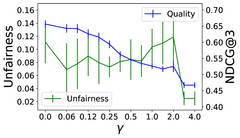
(b) DELTR, TREC

(c) FA*IR, TREC

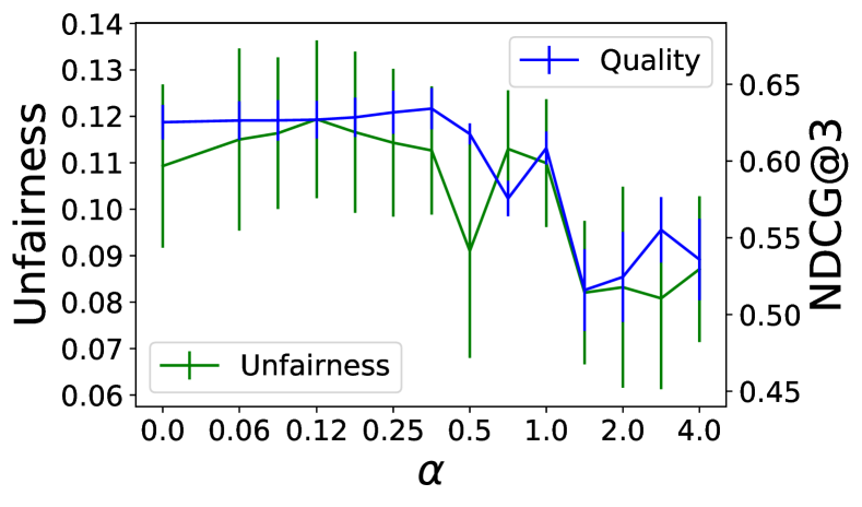
(d) Per-query, TREC

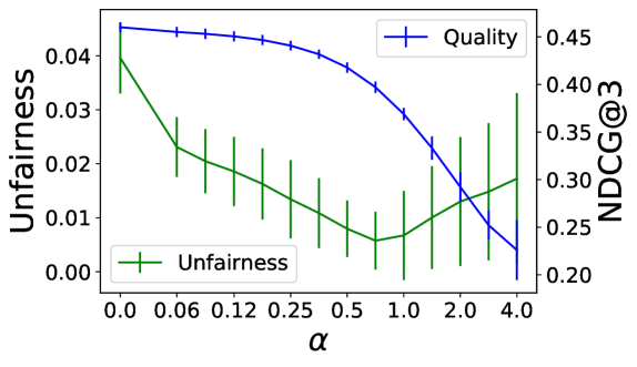
(e) Ours, MSMARCO

(f) FA*IR, MSMARCO

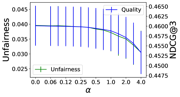
(g) Per-query, MSMARCO

Figure 1: Test-time performance of fair rankers with equal opportunity fairness, achieved by our algorithm and the baselines: unfairness (left $y$-axes) and NDCG@3 ranking quality (right $y$-axes); after training with different regularization strengths ($x$-axis). See the supplementary material for larger versions and for results for demographic parity and equalized odds.

5.2 Learning to rank models

Our algorithm.  We adopt a classical pointwise LTR approach with a generalized linear score function, $s(d,q)=\langle\theta,\phi(q,d)\rangle$, for a predefined feature function, $\phi:\mathcal{Q}\times\mathcal{D}\to\mathbb{R}^{D}$ (see supplemental material). As loss function of ranking quality, $L(s,S)$, we use the squared loss between the relevance labels and the predictions of $s$ over all data. To optimize for both ranking quality and fairness, we train with a weighted loss, as in equation (11). For TREC we train all models by $1500$ steps of gradient descent with a learning rate of $0.003$. In the MSMARCO experiments we train with $5$ epochs of SGD with a batch size of $100$ queries and $10$ passages per query and a learning rate of $0.0001$.

Baselines and ablation studies.  Our method is the first to enforce the well-established fairness notions from classification in a LTR setting. Hence previously developed methods for fair ranking aim to optimize for other (often single-purporse) fairness notions. Nevertheless, it is informative to see how such algorithms perform against our method, in order to understand the relationship between ours and previous fair ranking works. Therefore, we consider two recent methods for fair ranking, DELTR [74] and FA*IR [75], using the implementation provided by the authors [76].

DELTR is a state-of-the-art algorithm for fair LTR. At train time, a linear version of ListNet is trained, together with a regularizer tailored to a notion of disparate exposure [17, 56]. We use the same feature representations as for our method, as well as the same range for their regularization parameter $\gamma$, to ensure a fair comparison. Unfortunately, the implementation of [76] does not scale to MSMARCO.

FA*IR, on the other hand, is an algorithm that changes the ranking query by query, at prediction time, by ensuring that whenever $k$ items are retrieved, the proportion of retrieved items from a protected group is not smaller that the $\alpha$-th quantile of a binomial distribution $Bin(k,p)$, for fixed parameters $p,\alpha\in[0,1]$. We use $\alpha=0.1$ and $p\in[0.02,0.04,\ldots,0.98]$. Note that in our LTR setting the true relevances of items at test time are unknown, so we first train via our method with $\alpha=0$ and then, at test time, use the relevances predicted by our method as ground truth and apply FA*IR on top.

We also perform an ablation study by considering a version of our algorithm that learns to enforce fairness on the per-query level. This is inspired by [55], who, however, do not propose an algorithm for enforcing such per-query fairness notions. Within our framework this is achieved by regularizing with a separate term for every query in a batch and then averaging over the batch afterwards.

5.3 Results

Figure 1 shows the results when imposing different amounts of the equal opportunity fairness in typical settings for TREC ($t=3,k=3$; top row) and MSMARCO (com, $k=3$; bottom row). We also report the ranking quality and equal opportunity unfairness for the three baselines. As one can see, our method is able to consistently improve fairness. For TREC, this comes at no loss in ranking quality (here NDCG). For MSMARCO the loss is quite small for small to medium values of $\alpha$. As the figure shows, these observations are robust across the different amounts of regularization. In contrast, the fairness curves of the baselines behave erratically with respect to the trade-off parameters.

The possibility of increasing the fairness of learning models without damaging their accuracy has been previously observed in the context of supervised learning [66]. To the best of our knowledge, we are the first to observe this in a ranking context. This effect is more expressed in the experiment on the TREC data than for MSMARCO, possibly due to the higher number of relevant items per query in TREC, which results in more flexibility to rearrange items without decreasing the ranking quality.

Table 1: Maximal and mean relative fairness increase, achievable without a significant decrease of ranking quality, for our algorithm and the baselines. See main text for details.

TREC		Ours		DELTR		FA*IR		Per-query
		Max	Mean	Max	Mean	Max	Mean	Max	Mean
equality of opportunity	$t=3$	48%	34%	39%	23%	56%	18%	19%	-5%
	$t=4$	46%	37%	2%	-8%	56%	11%	14%	-4%
	$t=5$	46%	32%	18%	7%	6%	-17%	8%	-13%
demographic parity	$t=3$	27%	17%	55%	36%	83%	24%	15%	-1%
	$t=4$	44%	32%	12%	6%	56%	10%	27%	5%
	$t=5$	57%	40%	26%	14%	11%	-35%	24%	1%
equalized odds	$t=3$	20%	13%	48%	31%	57%	16%	14%	-3%
	$t=4$	30%	21%	9%	4%	40%	3%	13%	-1%
	$t=5$	29%	21%	21%	12%	0%	-35%	7%	-4%
average		39%	27%	26%	14%	41%	-1%	16%	-3%
MSMARCO		Ours		DELTR		FA*IR		Per-query
		Max	Mean	Max	Mean	Max	Mean	Max	Mean
equality of opportunity	com	55%	36%	NA	NA	64%	11%	24%	6%
	ext	19%	10%	NA	NA	0%	-112%	2%	0%
demographic parity	com	42%	27%	NA	NA	39%	-50%	0%	0%
	ext	20%	13%	NA	NA	0%	-168%	7%	3%
equalized odds	com	61%	41%	NA	NA	45%	-12%	14%	4%
	ext	28%	17%	NA	NA	0%	-142%	1%	0%
average		37%	24%	NA	NA	25%	-79%	8%	2%

We obtained very similar results also for the other setups, e.g. different values of $k$, fairness measures and protected attributes and for $\operatorname{P@k}$. Plots for these can be found in the supplemental material. Table 1 summarizes some of the results in a compact form. For different fairness notions and splits into protected groups (rows), it reports the maximal and mean reduction of the fairness violation measure over the range of values of the trade-off parameter for which the corresponding model’s prediction quality is not significantly worse than for a model trained without a fairness regularizer (i.e. $\alpha=0$). Here we call a model significantly worse than another if the difference of the mean quality values of the two models is larger than the sum of the standard errors/deviations, for TREC/MSMARCO respectively, around those averages (that is, if the error bars, as in Figure 1, would not intersect). The results are averaged over $k\in\{1,2,3,4,5\}$, with individual versions in the supplementary material.

Intuitively, the max values quantify how much an algorithm can improve fairness without decreasing the ranking quality, while the mean values report the average improvement of fairness over the values of the trade-off parameters, as a more robust measure. The results confirm that in all cases our proposed training method is able to greatly reduce the unfairness in the test time ranking without majorly damaging ranking quality. In comparison, the baselines behave inconsistently between experiments and are less robust to the choice of the trade-off parameter, indicating that training with the right regularization, as integrated in our method, is indeed beneficial for test time fairness.

We refer to the supplementary material for further results, including splits over the values of $k$, experiments for $\operatorname{P@k}$ and plots of the performance of our algorithm in other scenarios.

6 Conclusion

We introduced a framework for transferring classification fairness notions to the context of LTR, by rephrasing ranking as a collection of query-dependent classification problems. This viewpoint, while technically elementary, opens a wide range of possibilities for expanding the optimization methods and proof techniques from the fair classification literature to ranking and multi-label learning. In particular, we report the first – to our knowledge – generalization bound for group fairness in the context of ranking. We further show in our experiments that including a suitable regularizer during training can greatly improve the fairness of rankings with no or minor reduction in model quality. This effect seems even more pronounced than what had been observed in classification tasks, especially if the set of relevant items for any query is large. Therefore, we hypothesize that the multi-label nature of the ranking task naturally allows for more fairness without adverse effects on accuracy, and we deem making this intuition formal an interesting direction for future research.

Supplementary Material

The supplementary material is structured as follows:

Section A contains the complete proof of Theorem 1. In particular, Section A.1 discusses the chromatic concentration bounds of [31] that we need to address the dependence between the samples. Section A.2 uses this tool and a conditional probability concentration technique of [68] to prove a concentration bound for a single classifier. Finally, in Section A.3 we make this bound uniform over the hypothesis space by evoking a variant of the classic symmetrization argument (e.g. [63]), while carefully accounting for the dependence between the samples. We conclude with a brief discussion in Section A.4 on the bounds and with some ideas for potential improvements and extensions of the theoretical analysis.

Section B provides more technical details on our experiments, in particular on the feature extraction procedures used and on the computational costs.

Section C contains further experimental results, including results for $\operatorname{P@k}$ (Section C.1), results for all three fairness measures in the setup of Figure 1 (Section C.2), splits of Table 1 according to the value of $k$ (Section C.3) and the plots of the performance of our algorithm on all experimental setups (Section C.4).

Appendix A Proof of Theorem 1

To prove Theorem 1, we first introduce some classic definitions and concentration results for sums of dependent random variables from [31] in Section A.1. Next we show in Section A.2 how these can be used to derive large deviation bounds for the three fairness notions, given a fixed classifier. The proof is similar to the corresponding i.i.d. result of [68], however an application of the results from [31] is needed because of the dependence between the samples. Finally, in Section A.3 we show how these bounds can be made uniform over the hypothesis space by adapting the classic symmetrization argument (e.g. [63]) to a dependent data scenario.

A.1 Concentration inequalities for sums of dependent random variables

To deal with the dependence between the samples, we will use the following framework from [31]. Let $Y_{\alpha}$ be a set of random variables, with $\alpha$ ranging over some index set $\mathcal{A}$. Let $X=\sum_{\alpha\in\mathcal{A}}Y_{\alpha}$. To derive concentration bounds for $X$, the following notions are useful:

Definition 8 ([31]).

Given $\mathcal{A}$ and $\{Y_{\alpha}\}_{\alpha\in\mathcal{A}}$:

• A subset $\mathcal{A}^{\prime}\subset\mathcal{A}$ is independent if the random variables $\{Y_{\alpha}\}_{\alpha\in\mathcal{A}^{\prime}}$ are (jointly) independent.

• A family $\{\mathcal{A}_{j}\}_{j}$ is a cover of $\mathcal{A}$ if $\cup_{j}\mathcal{A}_{j}=\mathcal{A}$. A cover is proper if each set $\mathcal{A}_{j}$ is independent.

• $\chi(\mathcal{A})$ is the size of the smallest proper cover of $\mathcal{A}$, that is the smallest integer $m$, such that $\mathcal{A}$ can be written as the union of $m$ independent subsets.

Then the following result holds, similar to the Hoeffding inequality, but accounting for the amount of dependence between the random variables $\{Y_{\alpha}\}_{\alpha\in\mathcal{A}}$:

Theorem 2 ([31]).

Let $Y_{\alpha}$ and $X$ be as above, with $a_{\alpha}\leq Y_{\alpha}\leq b_{\alpha}$ for every $\alpha\in\mathcal{A}$, for some real numbers $a_{\alpha}$ and $b_{\alpha}$. Then, for every $t>0$:

$$\mathbb{P}(X\geq\mathbb{E}(X)+t)\leq\exp\left(-2\frac{t^{2}}{\chi(\mathcal{A})\sum_{\alpha\in\mathcal{A}}(b_{\alpha}-a_{\alpha})^{2}}\right).$$ (12)

The same upper bound holds for $\mathbb{P}(X\leq\mathbb{E}(X)-t)$.

If instead one considers the mean of $\{Y_{\alpha}\}_{\alpha\in\mathcal{A}}$, namely $\bar{X}=\frac{1}{|\mathcal{A}|}\sum_{\alpha\in\mathcal{A}}Y_{\alpha}$, then the following holds:

$$\mathbb{P}(\bar{X}\geq\mathbb{E}(\bar{X})+t)\leq\exp\left(-2\frac{t^{2}|\mathcal{A}|^{2}}{\chi(\mathcal{A})\sum_{\alpha\in\mathcal{A}}(b_{\alpha}-a_{\alpha})^{2}}\right).$$ (13)

Specifically, if the $Y_{\alpha}$ are Bernoulli random variables:

$$\mathbb{P}(\bar{X}\geq\mathbb{E}(\bar{X})+t)\leq\exp\left(-2\frac{t^{2}|\mathcal{A}|}{\chi(\mathcal{A})}\right).$$ (14)

A.2 Non-uniform bounds

First we use the tools from the previous section and a technique of [68, 2] to show a non-uniform Hoeffding-type bound for equal opportunity and equalized odds:

Lemma 1.

Fix $\delta\in(0,1)$ and a binary predictor $f:Q\times D\to\{0,1\}$. Suppose that $N>\frac{8\log(8/\delta)}{P^{2}}$, where $P=\min_{ar}\mathbb{P}(A(d)=a,r(q,d)=r)$, then:

$$\mathbb{P}\left(|\Gamma^{\textrm{EOp}}(f,S)-\Gamma^{\textrm{EOp}}(f)|>2\sqrt{\frac{\log(8/\delta)}{NP}}\right)\leq\delta.$$ (15)

and

$$\mathbb{P}\left(|\Gamma^{\textrm{EOd}}(f,S)-\Gamma^{\textrm{EOd}}(f)|>2\sqrt{\frac{\log(16/\delta)}{NP}}\right)\leq\delta.$$ (16)

Proof.

Denote by $I_{ar}=\{(i,j):A(d^{i}_{j})=a,r(q_{i},d^{i}_{j})=r\}$ the set of indexes of the training data for which the document belongs to the group $a$ and the relevance of the query-document pair is $r$. Notice that $I_{ar}$ is a random variable and that $|I_{ar}|=|S_{a,r}|$. We first bound the probability of a large deviation of

$$\gamma^{S}_{ar}(f)\vcentcolon=\frac{1}{|I_{ar}|}\sum_{(i,j)\in I_{ar}}f(q_{i},d^{i}_{j})$$

from $\gamma_{ar}(f)\vcentcolon=\mathbb{P}(f(q,d)=1|A(d)=a,r(q,d)=r)$, for each pair $r\in\{0,1\},a\in\{0,1\}$. Since $f$ is fixed here, we omit the dependence of $\gamma_{ar}(f),\gamma^{S}_{ar}(f),\Gamma^{\textrm{EOp}}(f),\Gamma^{\textrm{EOd}}(f)$, etc. on $f$ for the rest of this proof.

For any fixed $I_{ar}$:

$$\mathbb{E}\left(\gamma^{S}_{ar}|I_{ar}\right)=\mathbb{E}\left(\frac{1}{|I_{ar}|}\sum_{(i,j)\in I_{ar}}f(q_{i},d^{i}_{j})\right)=\mathbb{P}(f(q,d)=1|A(d)=a,r(q,d)=r)=\gamma_{ar}(f),$$ (17)

since the marginal distribution of every $(q_{i},d^{i}_{j},r(q_{i},d^{i}_{j}))$ is $\mathbb{P}$. It is also easy to see that if $\mathcal{A}=\{(i,j):i\in[N],j\in[m]\}$ is the index set of the random variables $Y_{(i,j)}=f(q_{i},d^{i}_{j})$, then $\chi(\mathcal{A})=m$. Therefore, for any fixed set $I_{ar}\subset\mathcal{A}$, we have $\chi(I_{ar})\leq\chi(\mathcal{A})=m$. Now conditional on $I_{ar}$:

$$\mathbb{E}(|\gamma^{S}_{ar}-\gamma_{ar}|>t|I_{ar})=\mathbb{E}\left(\left|\frac{1}{|I_{ar}|}\sum_{(i,j)\in I_{ar}}f(q_{i},d^{i}_{j})-\gamma_{ar}\right|>t\right)\leq 2\exp\left(-2\frac{t^{2}|I_{ar}|}{m}\right).$$ (18)

Similarly, $|I_{ar}|=\sum_{i\in[N]}\sum_{j\in[m]}\mathbbm{1}(r(q_{i},d^{i}_{j})=r,A(d^{i}_{j})=a)$ is the sum of $Nm$ Bernoulli random variables indexed by $\mathcal{A}=\{(i,j)\}_{i\in[N],j\in[m]}$, such that $\chi(\mathcal{A})=m$. Denote by $P_{ar}=\mathbb{P}(A(d)=a,r(q,d)=r)$ and recall the notation $P=\min_{ar}P_{ar}$. Then $\mathbb{E}(|I_{ar}|)=P_{ar}Nm$. Therefore,

$$\mathbb{P}\left(|I_{ar}|\leq P_{ar}Nm-t\right)\leq\exp\left(-2\frac{t^{2}}{Nm^{2}}\right).$$

Setting $t=P_{ar}Nm/2$, we obtain:

$$\mathbb{P}\left(|I_{ar}|\leq\frac{P_{ar}}{2}Nm\right)\leq\exp\left(-\frac{P^{2}_{ar}N}{2}\right).$$ (19)

Now assume that $N\geq\frac{2\log(8/\delta)}{P^{2}}$. Then for any $r\in\{0,1\},a\in\{0,1\}$:

$$\mathbb{P}(|\gamma^{S}_{ar}-\gamma_{ar}|>t) =\sum_{I_{ar}}\mathbb{P}(|\gamma^{S}_{ar}-\gamma_{ar}|>t|I_{ar})\mathbb{P}(I_{ar})$$

$$\leq\mathbb{P}(|I_{ar}|\leq\frac{P_{ar}}{2}Nm)+\sum_{I_{ar}:|I_{ar}|\geq\frac{P_{ar}Nm}{2}}\mathbb{P}(|\gamma^{S}_{ar}-\gamma_{ar}|>t|I_{ar})\mathbb{P}(I_{ar})$$

$$\leq\exp\left(-\frac{P^{2}_{ar}N}{2}\right)+\sum_{I_{ar}:|I_{ar}|\geq\frac{P_{ar}Nm}{2}}2\exp\left(-2\frac{t^{2}|I_{ar}|}{m}\right)\mathbb{P}(S_{ar})$$

$$\leq\frac{\delta}{8}+2\exp\left(-t^{2}NP_{ar}\right).$$

The rest of the proof proceeds as in [68]. For a fixed $r\in\{0,1\}$ the triangle law gives:

$$||\gamma^{S}_{0r}-\gamma^{S}_{1r}|-|\gamma_{0r}-\gamma_{1r}||\leq|\gamma^{S}_{0r}-\gamma^{S}_{1r}-\gamma_{0r}+\gamma_{1r}|\leq|\gamma^{S}_{0r}-\gamma_{0r}|+|\gamma^{S}_{1r}-\gamma_{1r}|.$$

Therefore,

$$\mathbb{P}(||\gamma^{S}_{0r}-\gamma^{S}_{1r}|-|\gamma_{0r}-\gamma_{1r}||>2t) \leq\mathbb{P}(|\gamma^{S}_{0r}-\gamma_{0r}|+|\gamma^{S}_{1r}-\gamma_{1r}|>2t)$$

$$\leq\mathbb{P}((|\gamma^{S}_{0r}-\gamma_{0r}|>t)\lor(|\gamma^{S}_{1r}-\gamma_{1r}|>t))$$

$$\leq\mathbb{P}(|\gamma^{S}_{0r}-\gamma_{0r}|>t)+\mathbb{P}(|\gamma^{S}_{1r}-\gamma_{1r}|>t)$$

$$\leq\frac{\delta}{4}+4\exp(-t^{2}NP).$$

Setting $t=t_{0}=\sqrt{\frac{\log(16/\delta)}{NP}}$ gives:

$$\mathbb{P}\left(||\gamma^{S}_{0r}-\gamma^{S}_{1r}|-|\gamma_{0r}-\gamma_{1r}||>2\sqrt{\frac{\log(16/\delta)}{NP}}\right)\leq\frac{\delta}{4}+4\frac{\delta}{16}=\frac{\delta}{2}.$$

Setting $r=1$ gives the first result.

For the second result, note that taking the union bound over $r\in\{0,1\}$ shows that with probability at least $1-\delta$ both $||\gamma^{S}_{00}-\gamma^{S}_{10}|-|\gamma_{00}-\gamma_{10}||\leq 2t_{0}$ and $||\gamma^{S}_{01}-\gamma^{S}_{11}|-|\gamma_{01}-\gamma_{11}||\leq 2t_{0}$ hold.

Under this event we have:

$$|\Gamma^{\textrm{EOd}}(f,S)-\Gamma^{\textrm{EOd}}(f)| =\left|\frac{1}{2}\left(|\gamma^{S}_{00}-\gamma^{S}_{10}|+|\gamma^{S}_{01}-\gamma^{S}_{11}|\right)-\frac{1}{2}\left(|\gamma_{00}-\gamma_{10}|+|\gamma_{01}-\gamma_{11}|\right)\right|$$

$$=\left|\frac{1}{2}\left(|\gamma^{S}_{00}-\gamma^{S}_{10}|-|\gamma_{00}-\gamma_{10}|\right)+\frac{1}{2}\left(|\gamma^{S}_{01}-\gamma^{S}_{11}|-|\gamma_{01}-\gamma_{11}|\right)\right|$$

$$\leq\frac{1}{2}\left||\gamma^{S}_{00}-\gamma^{S}_{10}|-|\gamma_{00}-\gamma_{10}|\right|+\frac{1}{2}\left||\gamma^{S}_{01}-\gamma^{S}_{11}|-|\gamma_{01}-\gamma_{11}|\right|$$

$$\leq 2t_{0}$$

and hence the result follows. ∎

An identical argument, by conditioning on the values of the set $I_{a}=\{(i,j):A(d^{i}_{j})=a\}$ gives a similar result for demographic parity:

Lemma 2.

Fix $\delta\in(0,1)$ and a binary predictor $f:Q\times D\to\{0,1\}$. Suppose that $N>\frac{8\log(8/\delta)}{Q^{2}}$, where $Q=\min_{a}\mathbb{P}(A(d)=a)$, then:

$$\mathbb{P}\left(|\Gamma^{\textrm{DP}}(f,S)-\Gamma^{\textrm{DP}}(f)|>2\sqrt{\frac{\log(8/\delta)}{NQ}}\right)\leq\delta.$$ (20)

A.3 Uniform bounds

In this section we show how to formally extend the non-uniform bounds from the previous section to hold uniformly over the hypothesis space $\mathcal{H}$.

Let $S^{\prime}=\{(q^{\prime}_{i},d^{\prime i}_{j},r(q^{\prime}_{i},d^{\prime i}_{j}))\}_{i\in[N],j\in[m]}$ be a ghost sample independent of $S$ and also sampled via the same procedure as $S$, as described in the main body of the paper. In the proof of Lemma 1 we showed that for any classifier $f$ and any $t\in(0,1)$:

$$\mathbb{P}\left(|\Gamma^{\textrm{EOp}}(f)-\Gamma^{\textrm{EOp}}(f,S)|>2t\right)\leq 2\exp\left(-\frac{P^{2}N}{2}\right)+4\exp\left(-\frac{t^{2}NP}{2}\right)\leq 6\exp\left(-\frac{t^{2}NP^{2}}{2}\right)$$ (21)

$$\mathbb{P}\left(|\Gamma^{\textrm{EOd}}(f)-\Gamma^{\textrm{EOd}}(f,S)|>2t\right)\leq 4\exp\left(-\frac{P^{2}N}{2}\right)+8\exp\left(-\frac{t^{2}NP}{2}\right)\leq 12\exp\left(-\frac{t^{2}NP^{2}}{2}\right)$$ (22)

Similarly, from the proof of Lemma 2

$$\mathbb{P}\left(|\Gamma^{\textrm{DP}}(f)-\Gamma^{\textrm{DP}}(f,S)|>2t\right)\leq 2\exp\left(-\frac{Q^{2}N}{2}\right)+4\exp\left(-\frac{t^{2}NQ}{2}\right)\leq 6\exp\left(-\frac{t^{2}NQ^{2}}{2}\right)$$ (24)

We will use these in particular to prove the following symmetrization lemma:

Lemma 3.

For any $1>t\geq 4\sqrt{\frac{2\log(12)}{NP^{2}}}$,

$$\mathbb{P}_{S}\left(\sup_{f\in\mathcal{F}}(\Gamma^{\textrm{EOp}}(f)-\Gamma^{\textrm{EOp}}(f,S))\geq t\right)\leq 2\mathbb{P}_{S,S^{\prime}}\left(\sup_{f\in\mathcal{F}}(\Gamma^{\textrm{EOp}}(f,S^{\prime})-\Gamma^{\textrm{EOp}}(f,S))\geq t/2\right).$$ (25)

For any $1>t\geq 4\sqrt{\frac{2\log(24)}{NP^{2}}}$:

$$\mathbb{P}_{S}\left(\sup_{f\in\mathcal{F}}(\Gamma^{\textrm{EOd}}(f)-\Gamma^{\textrm{EOd}}(f,S))\geq t\right)\leq 2\mathbb{P}_{S,S^{\prime}}\left(\sup_{f\in\mathcal{F}}(\Gamma^{\textrm{EOd}}(f,S^{\prime})-\Gamma^{\textrm{EOd}}(f,S))\geq t/2\right).$$ (26)

For any $1>t\geq 4\sqrt{\frac{2\log(12)}{NQ^{2}}}$:

$$\mathbb{P}_{S}\left(\sup_{f\in\mathcal{F}}(\Gamma^{\textrm{DP}}(f)-\Gamma^{\textrm{DP}}(f,S))\geq t\right)\leq 2\mathbb{P}_{S,S^{\prime}}\left(\sup_{f\in\mathcal{F}}(\Gamma^{\textrm{DP}}(f,S^{\prime})-\Gamma^{\textrm{DP}}(f,S))\geq t/2\right).$$ (27)

Proof.

We show the result for the equal opportunity fairness measure, the rest follow in an identical manner.

Let $f^{*}$ be the function achieving the supremum on the left-hand side . Note that:

$$\mathbbm{1}(\Gamma^{\textrm{EOp}}(f^{*})-\Gamma^{\textrm{EOp}}(f^{*},S)\geq t) \mathbbm{1}(\Gamma^{\textrm{EOp}}(f^{*})-\Gamma^{\textrm{EOp}}(f^{*},S^{\prime})<t/2)$$

$$=\mathbbm{1}(\Gamma^{\textrm{EOp}}(f^{*})-\Gamma^{\textrm{EOp}}(f^{*},S)\geq t\wedge\Gamma^{\textrm{EOp}}(f^{*},S^{\prime})-\Gamma^{\textrm{EOp}}(f^{*})>-t/2)$$

$$\leq\mathbbm{1}(\Gamma^{\textrm{EOp}}(f^{*},S^{\prime})-\Gamma^{\textrm{EOp}}(f^{*},S)>t/2).$$

Taking expectation with respect to $S^{\prime}$:

$$\mathbbm{1}(\Gamma^{\textrm{EOp}}(f^{*})-\Gamma^{\textrm{EOp}}(f^{*},S)\geq t)\mathbb{P}_{S^{\prime}}(\Gamma^{\textrm{EOp}}(f^{*})-\Gamma^{\textrm{EOp}}(f^{*},S^{\prime})<t/2)\leq\mathbb{P}_{S^{\prime}}(\Gamma^{\textrm{EOp}}(f^{*},S^{\prime})-\Gamma^{\textrm{EOp}}(f^{*},S)>t/2).$$

Now using (21):

$$\mathbb{P}_{S^{\prime}}(\Gamma^{\textrm{EOp}}(f^{*})-\Gamma^{\textrm{EOp}}(f^{*},S^{\prime})\geq t/2)\leq 6\exp\left(-\frac{t^{2}NP^{2}}{32}\right)\leq\frac{1}{2},$$

so:

$$\frac{1}{2}\mathbbm{1}(\Gamma^{\textrm{EOp}}(f^{*})-\Gamma^{\textrm{EOp}}(f^{*},S)\geq t)\leq\mathbb{P}_{S^{\prime}}(\Gamma^{\textrm{EOp}}(f^{*},S^{\prime})-\Gamma^{\textrm{EOp}}(f^{*},S)>t/2).$$

Taking expectation with respect to $S$:

$$\mathbb{P}_{S}(\Gamma^{\textrm{EOp}}(f^{*})-\Gamma^{\textrm{EOp}}(f^{*},S)\geq t) \leq 2\mathbb{P}_{S,S^{\prime}}(\Gamma^{\textrm{EOp}}(f^{*},S^{\prime})-\Gamma^{\textrm{EOp}}(f^{*},S)>t/2)$$

$$\leq 2\mathbb{P}_{S,S^{\prime}}(\sup_{f\in\mathcal{F}}(\Gamma^{\textrm{EOp}}(f,S^{\prime})-\Gamma^{\textrm{EOp}}(f,S))\geq t/2).$$

∎

Given a set of $n$ input datapoints $z_{1},\ldots,z_{n}$ with $z_{i}=(q_{i},d_{i},r(q_{i},d_{i}))$, consider:

$$\mathcal{F}_{z_{1},\ldots,z_{n}}=\{(f(q_{1},d_{1}),\ldots,f(q_{n},d_{n})):f\in\mathcal{F}\}$$ (28)

Then the growth function of $\mathcal{F}$ is defined as:

$$S_{\mathcal{F}}(n)=\sup_{(z_{1},\ldots,z_{n})}|\mathcal{F}_{z_{1},\ldots,z_{n}}|$$ (29)

We can now present a proof of Theorem 1:

Theorem 1.

Suppose that $v=VC(\mathcal{F})\geq 1$ and that $2Nm>v$. Then for any $\delta\in(0,1)$:

$$\mathbb{P}_{S}\left(\sup_{f\in\mathcal{F}}(\Gamma^{\textrm{EOp}}(f)-\Gamma^{\textrm{EOp}}(f,S))\geq 8\sqrt{2\frac{d\log(\frac{2eNm}{d})+\log(\frac{24}{\delta})}{NP^{2}}}\right)\leq\delta$$ (30)

$$\mathbb{P}_{S}\left(\sup_{f\in\mathcal{F}}(\Gamma^{\textrm{DP}}(f)-\Gamma^{\textrm{DP}}(f,S))\geq 8\sqrt{2\frac{d\log(\frac{2eNm}{d})+\log(\frac{24}{\delta})}{NQ^{2}}}\right)\leq\delta$$ (31)

$$\mathbb{P}_{S}\left(\sup_{f\in\mathcal{F}}(\Gamma^{\textrm{EOd}}(f)-\Gamma^{\textrm{EOd}}(f,S))\geq 8\sqrt{2\frac{d\log(\frac{2eNm}{d})+\log(\frac{48}{\delta})}{NP^{2}}}\right)\leq\delta$$ (32)

Proof.

Again we present the proof for equal opportunity, with the other inequalities following in an identical manner.

Note that given sets $S$ and $S^{\prime}$, the values of $\Gamma^{\textrm{EOp}}(f,S)$ and $\Gamma^{\textrm{EOp}}(f,S^{\prime})$ are completely determined by the values of $f$ on $S$ and $S^{\prime}$ respectively. Therefore, for any $t\in\left(4\sqrt{\frac{2\log(12)}{NP^{2}}},1\right)$ using Lemma 3 and the union bound:

$$\mathbb{P}_{S}\left(\sup_{f\in\mathcal{F}}(\Gamma^{\textrm{EOp}}(f)-\Gamma^{\textrm{EOp}}(f,S))\geq t\right) \leq 2\mathbb{P}_{S,S^{\prime}}\left(\sup_{f\in\mathcal{F}}(\Gamma^{\textrm{EOp}}(f,S^{\prime})-\Gamma^{\textrm{EOp}}(f,S))\geq t/2\right)$$

$$\leq 2S_{\mathcal{F}}(2Nm)\mathbb{P}_{S,S^{\prime}}\left(\Gamma^{\textrm{EOp}}(f,S^{\prime})-\Gamma^{\textrm{EOp}}(f,S)\geq t/2\right)$$

$$\leq 2S_{\mathcal{F}}(2Nm)\mathbb{P}_{S,S^{\prime}}\left((|\Gamma^{\textrm{EOp}}(f,S^{\prime})-\Gamma^{\textrm{EOp}}(f)|\geq t/4)\right.$$

$$\lor\left.(|\Gamma^{\textrm{EOp}}(f)-\Gamma^{\textrm{EOp}}(f,S)|\geq t/4)\right)$$

$$\leq 4S_{\mathcal{F}}(2Nm)\mathbb{P}_{S}\left(|\Gamma^{\textrm{EOp}}(f)-\Gamma^{\textrm{EOp}}(f,S)|\geq t/4\right)$$

$$\leq 24S_{\mathcal{F}}(2Nm)\exp\left(-\frac{t^{2}NP^{2}}{128}\right)$$

In particular, if $d=VC(\mathcal{F})$, by Sauer’s lemma $S_{\mathcal{F}}(2Nm)\leq\left(\frac{2eNm}{d}\right)^{d}$ whenever $2Nm>d$, so:

$$\mathbb{P}_{S}\left(\sup_{f\in\mathcal{F}}(\Gamma^{\textrm{EOp}}(f)-\Gamma^{\textrm{EOp}}(f,S))\geq t\right)\leq 24\left(\frac{2eNm}{d}\right)^{d}\exp\left(-\frac{t^{2}NP^{2}}{128}\right)$$

It follows that:

$$\mathbb{P}_{S}\left(\sup_{f\in\mathcal{F}}(\Gamma^{\textrm{EOp}}(f)-\Gamma^{\textrm{EOp}}(f,S))\geq 8\sqrt{2\frac{d\log(\frac{2eNm}{d})+\log(\frac{24}{\delta})}{NP^{2}}}\right)\leq\delta$$ (33)

whenever:

$$1>8\sqrt{2\frac{d\log(\frac{2eNm}{d})+\log(\frac{24}{\delta})}{NP^{2}}}\geq 4\sqrt{\frac{2\log(12)}{NP^{2}}}$$

It is easy to see that the right inequality holds whenever $d\geq 1$, $2Nm\geq d$ and $\delta<1$. In addition, inequality (33) trivially holds if the left inequality is not fulfilled. Hence the result follows. ∎

A.4 Discussion

Theorem 1 bounds the fairness violation on future data by the fairness on the training set plus an explicit complexity term, uniformly over all item selection functions. Consequently, any item selection function with low fairness violation on the training set will have a similarly low fairness violation on new data, provided that enough data was used for training. Indeed, the complexity term decreases like $\sqrt{\log N/N}$ as $N\to\infty$, which is the expected behavior for a VC-based bound.

The same scaling behavior does not hold with respect to the number of items per query, $m$. This is unfortunate, but unavoidable, given the weak assumptions we make on the data generation process: because we do not restrict how the per-query item sets are created, each of them could simply consist of many copies of a single item. In that case, even arbitrary large $m$ would provide only as much information as $m=1$. In the current form, $m$ appears even logarithmically in the numerator of the complexity term. We believe this to be an artifact of our proof technique, and expect that a more refined analysis will allow us to remove this dependence in the future.

Note that for real data, we do expect larger $m$ to be have a beneficial effect on generalization. This is the reason that we prefer to present the bound as it is in the theorem, i.e. with the empirical fairness estimated from all available data, rather than any alternative formulation, e.g. subsampling the training set to $m=1$, which would recover an i.i.d. setting. Finding an assumption on the generating process of real-world LTR data that does allow bounds that decrease with respect to $m$ is an interesting topic for future work.

In addition, we expect that more advanced techniques from learning theory, e.g. analysis based on Rademacher complexities [6], can be applied to obtain sharper, data-dependent guarantees. Indeed, there has been work on extending the classic Rademacher complexity generalization bounds to the case of dependent data, e.g. [62], and we deem the application of such techniques in the context of fair LTR an interesting direction for future work.

Appendix B Details of Experimental Setup

Here we present further details about our experiments, in particular the construction of the feature embeddings $\phi:\mathcal{Q}\times\mathcal{D}\to\mathbb{R}^{D}$ and a discussion on the computation costs of our experiments.

B.1 Feature extraction

TREC.  Inspired by the learning to rank approach for the TREC track of [12], we pre-compute $9$-dimensional embeddings of every query-paper pair by using the following hardcrafted features:

• the BM25 score of the query with the title, abstract, authors, topics and publication venue of the paper (5 values),

• the number of in- and out-citations (2 values),

• the publication year of the paper (1 value)

• the character length of the query (1 value).

Each feature is normalized by substracting the mean of the feature over the dataset and dividing by its standard deviation.

MSMARCO.  We use pretrained $768$-dimensional BERT feature embeddings [24] for representing the query-passage pairs. Specifically, we follow the embedding procedure described in [49, 29], where each query-passage pair is represented as the following token sequence:

$$[CLS]\text{ query text }[SEP]\text{ passage text }[CLS]$$

This sequence is then processed through a pre-trained BERT model from Tensorflow Hub [1], with maximum sequence length set to $200$, and the hidden units of the first $[CLS]$ token are used as a representation of the query-passage pair.

B.2 Computational costs

For both datasets running a single experiment consists of training and evaluating a single ML model, with a fixed choice of training method (algorithm), type of fairness, split into protected groups and value of the regularization parameter. In both cases, training an individual model was relatively cheap, with the main computational considerations coming from the large number of experiments to be ran in total.

For TREC an individual experiment takes about $60$ seconds on a CPU for our algorithm and for FA*IR and around $11$ and $17$ minutes for DELTR and the per-query baseline respectively. Each experiment requires less than $512$MB of RAM. In total, we ran $1170$ experiments for each of these algorithms, one for every fixed type of fairness (equality of opportunity, demographic parity or equalized odds), split into protected groups (3 types of splits, corresponding to $t=3,4,5$), value of the regularization parameter (a total of $26$ values were used), and a choice of a train-test split (a total of $5$ independent splits were used).

For MSMARCO an individual experiment takes about $9$ minutes on a CPU for our algorithm and for FA*IR and about $40$ minutes for the per-query method. Each experiment requires less than $64$GB of RAM. In total, we ran $960$ experiments for each of those models, one for every fixed type of fairness (equality of opportunity, demographic parity or equalized odds), split into protected groups (2 types of splits, com and ext), value of the regularization parameter (a total of $16$ values were used), and a choice of a train-test split (a total of $10$ random seeds were used to compute a random split).

Therefore, approximately $585$ and $928$ CPU hours are needed for the TREC and the MSMARCO experiments in total.

Appendix C Further experimental results

We report on multiple additional metrics and experiments on the TREC and MSMARCO data, that were deferred to the supplementary material for space reasons.

C.1 Results with $\operatorname{P@k}$

We first present plots from the same experiments as in Figure 1, but with Precision@k as a metric for model performance. Specifically, Figure 2 shows the results when imposing different amounts of the equal opportunity fairness notions in typical settings for TREC ($t=3,k=3$; top row) and MSMARCO (com, $k=3$; bottom row), both for our method and for the baselines. We see a very similar picture as with the NDCG metric, with no loss in precision for our method on the TREC data and little to no effect for MSMARCO, for small to medium values of $\alpha$. Again, the baselines are not able to consistently improve equal opportunity.

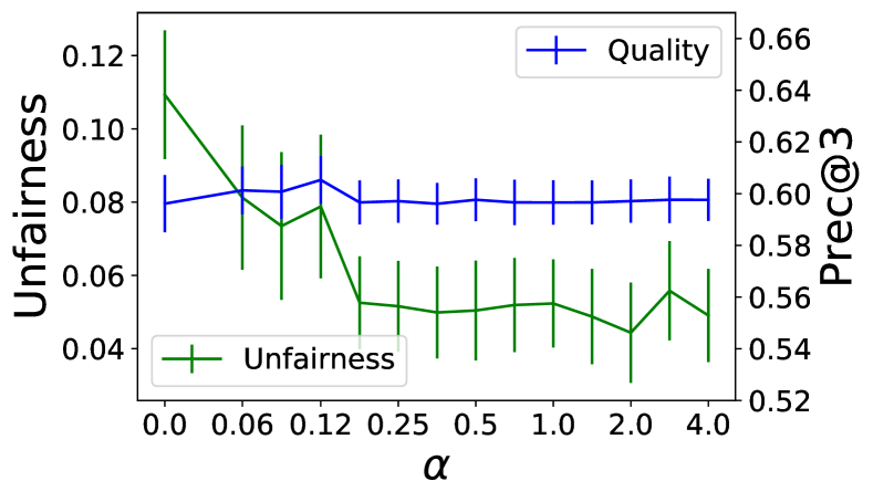
(a) Ours, TREC

(b) DELTR, TREC

(c) FA*IR, TREC

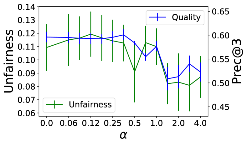
(d) Per-query, TREC

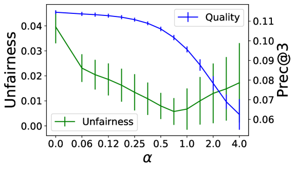
(e) Ours, MSMARCO

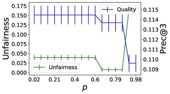
(f) FA*IR, MSMARCO

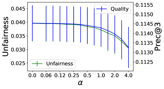
(g) Per-query, MSMARCO

Figure 2: Test-time performance of fair rankers with equal opportunity fairness, achieved by our algorithm and the baselines: unfairness (left $y$-axes) and Prec@3 ranking quality (right $y$-axes); after training with different regularization strengths ($x$-axis).

C.2 Plots for all three fairness measures

Here we present all results in the typical settings for TREC ($t=3,k=3$) on Figure 3 and for MSMARCO (com, $k=3$) on Figure 4. These plots complement Figure 1 from the main body of the paper by showing the results for the other two fairness measures, demographic parity and equalized odds, as well. We see that also for these measures our algorithm effectively improves fairness at little to no cost in ranking performance, for small values of $\alpha$. On the other hand, the baselines perform erratically and inconsistently across the measures and the two datasets.

(a) Ours, equal opportunity

(b) Ours, demographic parity

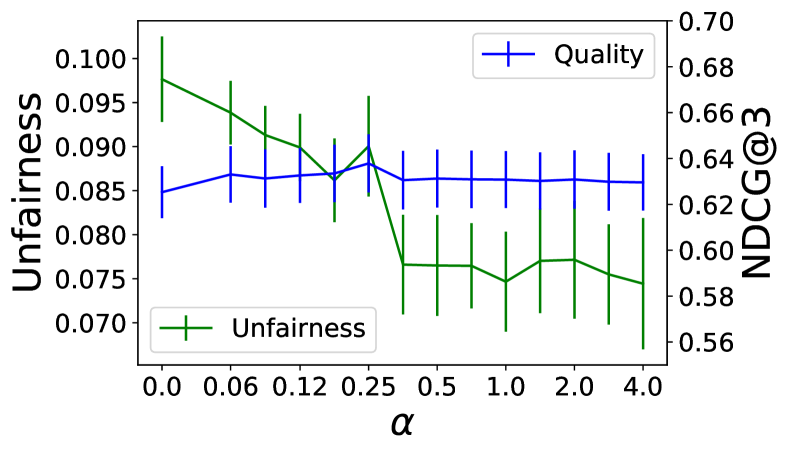
(c) Ours, equal odds

(d) DELTR, equal opportunity

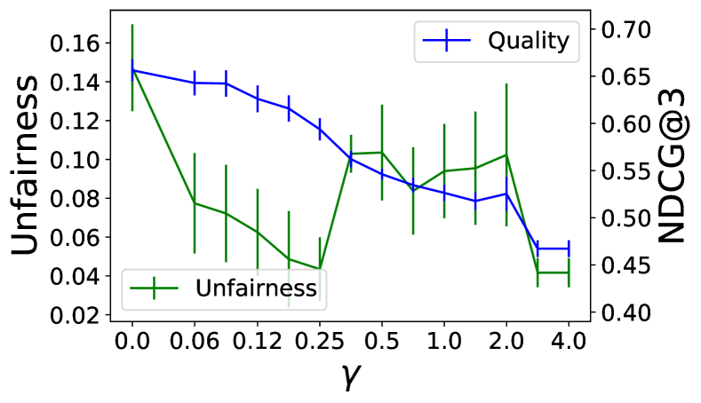
(e) DELTR, demographic parity

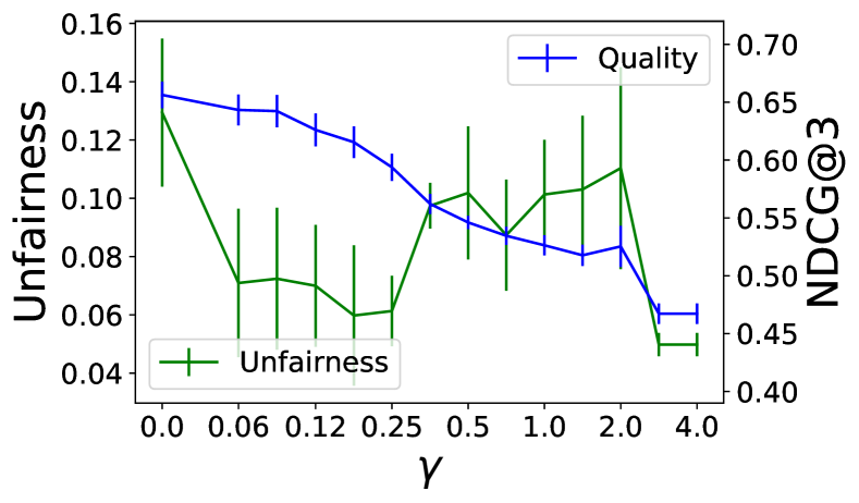
(f) DELTR, equal odds

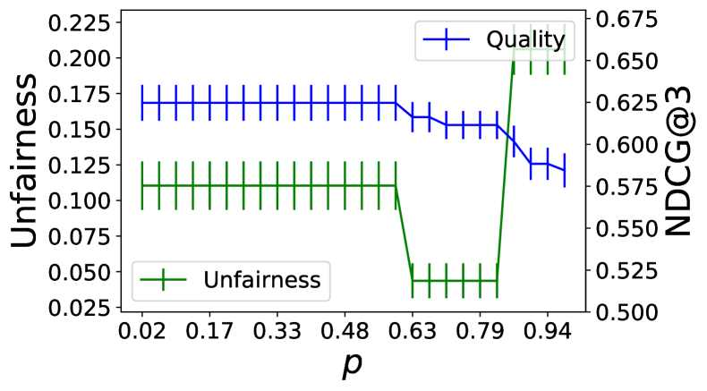
(g) FA*IR, equal opportunity

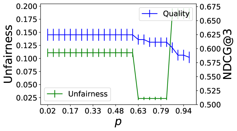
(h) FA*IR, demographic parity

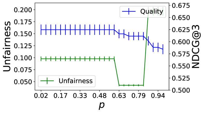
(i) FA*IR, equal odds

(j) Per-query, equal opportunity

(k) Per-query, demographic parity

(l) Per-query, equal odds

Figure 3: TREC: Test-time performance of fair rankers with equal opportunity, demographic parity and equalized odds fairness, achieved by our algorithm and the baselines: unfairness (left $y$-axes) and NDCG@3 ranking quality (right $y$-axes); after training with different regularization strengths ($x$-axis).

(a) Ours, equal opportunity

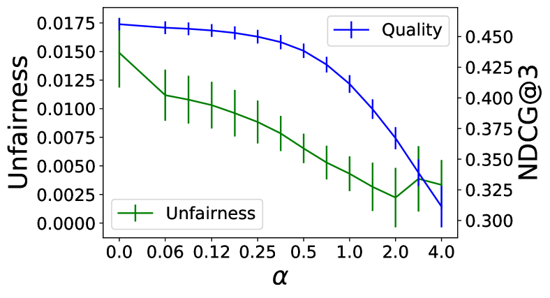
(b) Ours, demographic parity

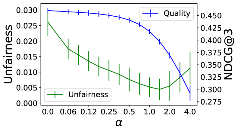
(c) Ours, equal odds

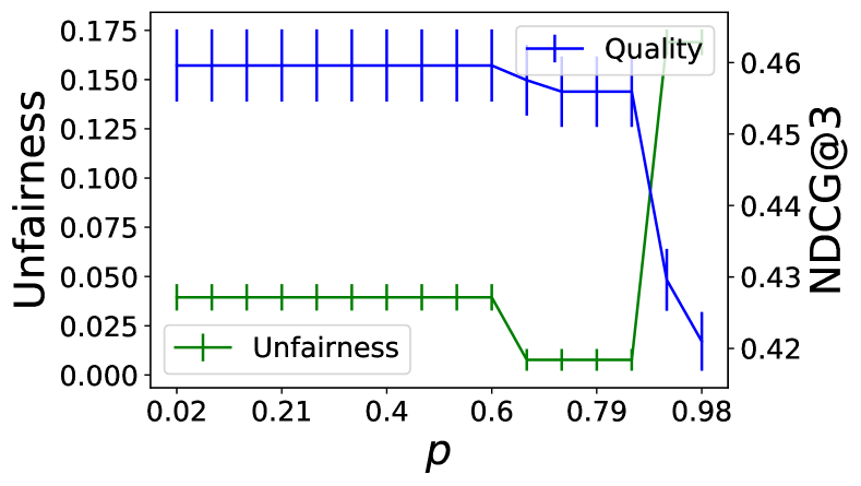
(d) FA*IR, equal opportunity

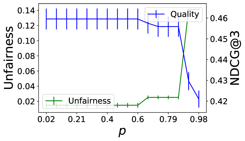
(e) FA*IR, demographic parity

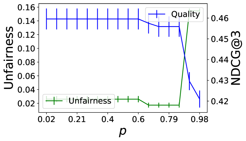
(f) FA*IR, equal odds

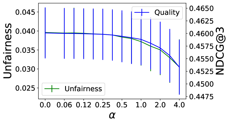
(g) Per-query, equal opportunity

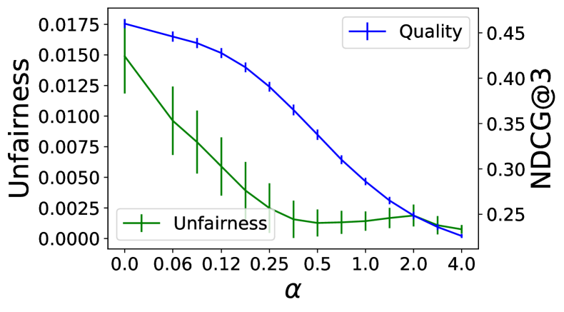
(h) Per-query, demographic parity

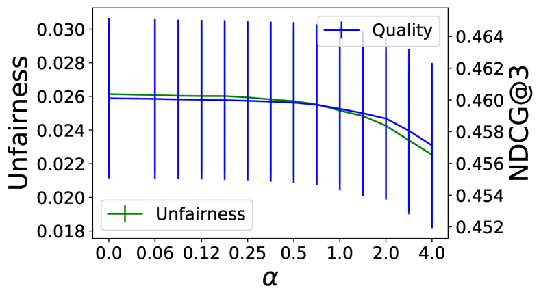
(i) Per-query, equal odds

Figure 4: MSMARCO: Test-time performance of fair rankers with equal opportunity, demographic parity and equalized odds fairness, achieved by our algorithm and the baselines: unfairness (left $y$-axes) and NDCG@3 ranking quality (right $y$-axes); after training with different regularization strengths ($x$-axis).

C.3 Mean and maximal improvements of fairness

Next we provide estimates on how much improvement of fairness is achievable without sacrificing ranking quality, both for our algorithm and the baselines. Essentially, we provide analogs of the results in Table 1, but with detailed splits according to the values of $k$.

Specifically, Tables 2, 3, 4, 5 report the maximal reduction of the fairness violation measure over the range of values of the trade-off parameter for which the corresponding model’s prediction quality is not significantly worse than for a model trained without a fairness regularizer (i.e. $\alpha=0$), for our method, DELTR, FAIR and the per-query fairness variant respectively. Recall that we call a model significantly worse than another if the difference of the mean quality values of the two models is larger than the sum of the standard errors/deviations, for TREC/MSMARCO respectively, around those averages (that is, if the error bars, as in Figure 1, would not intersect). Each of the entries in a table reports the improvement possible by the algorithm under consideration.

Next, Tables 6, 7, 8, 9 report the mean reduction of the fairness violation measure over the range of values of the trade-off parameter for which the corresponding model’s prediction quality is not significantly worse than for a model trained without a fairness regularizer (i.e. $\alpha=0$), again for our method, DELTR, FAIR and the per-query fairness variant respectively.

Table 2: Maximal relative fairness increase without a significant decrease of ranking quality for our method. See main text for details.

TREC		$k$					average
		1	2	3	4	5	over $k$
equality of opportunity	$t=3$	52%	58%	59%	37%	32%	48%
	$t=4$	51%	46%	42%	56%	36%	46%
	$t=5$	53%	55%	48%	48%	27%	46%
demographic parity	$t=3$	41%	31%	32%	17%	12%	27%
	$t=4$	65%	41%	45%	42%	30%	44%
	$t=5$	62%	43%	67%	61%	50%	57%
equalized odds	$t=3$	23%	24%	24%	13%	16%	20%
	$t=4$	32%	25%	31%	38%	24%	30%
	$t=5$	34%	10%	38%	42%	21%	29%
average over settings		46%	37%	43%	39%	27%	39%

MSMARCO		$k$					average
		1	2	3	4	5	over $k$
equality of opportunity	com	63%	58%	53%	49%	50%	55%
	ext	25%	24%	19%	19%	9%	19%
demographic parity	com	38%	41%	41%	46%	43%	42%
	ext	14%	16%	19%	22%	28%	20%
equalized odds	com	67%	63%	60%	58%	59%	61%
	ext	27%	29%	27%	30%	30%	28%
average over settings		39%	38%	36%	37%	36%	37%

Table 3: Maximal relative fairness increase without a significant decrease of ranking quality: DELTR method. See main text for details.

TREC		$k$					average
		1	2	3	4	5	over $k$
equality of opportunity	$t=3$	26%	43%	38%	49%	41%	39%
	$t=4$	10%	0%	0%	0%	0%	2%
	$t=5$	28%	20%	23%	18%	0%	18%
demographic parity	$t=3$	59%	66%	51%	50%	50%	55%
	$t=4$	22%	22%	11%	7%	0%	12%
	$t=5$	40%	30%	28%	20%	11%	26%
equalized odds	$t=3$	39%	53%	45%	54%	49%	48%
	$t=4$	19%	18%	4%	3%	0%	9%
	$t=5$	33%	26%	23%	18%	6%	21%
average over settings		31%	31%	25%	24%	17%	26%

Table 4: Maximal relative fairness increase without a significant decrease of ranking quality: FA*IR method. See main text for details.

TREC		$k$			average
		3	4	5	over $k$
equality of opportunity	$t=3$	60%	56%	53%	56%
	$t=4$	23%	78%	68%	56%
	$t=5$	0%	5%	13%	6%
demographic parity	$t=3$	79%	77%	93%	83%
	$t=4$	26%	67%	75%	56%
	$t=5$	0%	0%	33%	11%
equalized odds	$t=3$	56%	54%	60%	57%
	$t=4$	10%	48%	62%	40%
	$t=5$	0%	0%	1%	0%
average over settings		28%	43%	51%	41%

MSMARCO		$k$			average
		3	4	5	over $k$
equality of opportunity	com	80%	66%	44%	64%
	ext	0%	0%	0%	0%
demographic parity	com	0%	36%	80%	39%
	ext	0%	0%	0%	0%
equalized odds	com	33%	51%	51%	45%
	ext	0%	0%	0%	0%
average over settings		19%	26%	29%	25%

Table 5: Maximal relative fairness increase without a significant decrease of ranking quality: per query fairness. See main text for details.

TREC		$k$					average
		1	2	3	4	5	over $k$
equality of opportunity	$t=3$	28%	19%	17%	20%	9%	19%
	$t=4$	21%	0%	2%	29%	19%	14%
	$t=5$	9%	14%	10%	6%	0%	8%
demographic parity	$t=3$	4%	14%	22%	17%	17%	15%
	$t=4$	32%	26%	26%	25%	24%	27%
	$t=5$	48%	15%	35%	8%	15%	24%
equalized odds	$t=3$	16%	14%	7%	22%	11%	14%
	$t=4$	11%	3%	19%	14%	16%	13%
	$t=5$	7%	8%	11%	11%	0%	7%
average over settings		19%	13%	17%	17%	12%	16%

MSMARCO		$k$					average
		1	2	3	4	5	over $k$
equality of opportunity	com	28%	25%	23%	19%	23%	24%
	ext	3%	1%	5%	1%	2%	2%
demographic parity	com	0%	0%	0%	0%	0%	0%
	ext	4%	6%	8%	6%	9%	7%
equalized odds	com	16%	15%	14%	13%	14%	14%
	ext	1%	1%	2%	1%	2%	1%
average over settings		9%	8%	9%	7%	8%	8%

Table 6: Mean relative fairness increase without a significant decrease of ranking quality for our method.

TREC		$k$					average
		1	2	3	4	5	over $k$
equality of opportunity	$t=3$	29%	42%	44%	27%	26%	34%
	$t=4$	41%	38%	33%	44%	28%	37%
	$t=5$	35%	28%	41%	40%	18%	32%
demographic parity	$t=3$	30%	20%	21%	8%	9%	17%
	$t=4$	49%	26%	32%	30%	23%	32%
	$t=5$	43%	21%	56%	42%	39%	40%
equalized odds	$t=3$	16%	14%	15%	7%	11%	13%
	$t=4$	25%	18%	20%	27%	17%	21%
	$t=5$	23%	6%	28%	29%	17%	21%
average over settings		32%	24%	32%	28%	21%	27%

MSMARCO		$k$					average
		1	2	3	4	5	over $k$
equality of opportunity	com	42%	39%	36%	33%	33%	36%
	ext	12%	12%	9%	10%	5%	10%
demographic parity	com	24%	26%	27%	30%	29%	27%
	ext	10%	11%	12%	13%	17%	13%
equalized odds	com	44%	41%	39%	38%	40%	41%
	ext	16%	17%	15%	18%	18%	17%
average over settings		25%	24%	23%	24%	24%	24%

Table 7: Mean relative fairness increase without a significant decrease of ranking quality: DELTR method.

TREC		$k$					average
		1	2	3	4	5	over $k$
equality of opportunity	$t=3$	10%	26%	23%	28%	27%	23%
	$t=4$	5%	-2%	-9%	-12%	-23%	-8%
	$t=5$	15%	10%	11%	9%	-11%	7%
demographic parity	$t=3$	43%	45%	33%	31%	30%	36%
	$t=4$	11%	11%	5%	3%	-1%	6%
	$t=5$	25%	15%	14%	10%	5%	14%
equalized odds	$t=3$	24%	40%	30%	33%	30%	31%
	$t=4$	9%	9%	2%	2%	-3%	4%
	$t=5$	21%	13%	12%	9%	3%	12%
average over settings		18%	19%	13%	13%	7%	14%

Table 8: Mean relative fairness increase without a significant decrease of ranking quality: FA*IR method.

TREC		$k$			average
		3	4	5	over $k$
equality of opportunity	$t=3$	16%	17%	20%	18%
	$t=4$	-1%	7%	26%	11%
	$t=5$	-24%	-25%	-2%	-17%
demographic parity	$t=3$	22%	20%	29%	24%
	$t=4$	1%	3%	26%	10%
	$t=5$	-37%	-52%	-16%	-35%
equalized odds	$t=3$	15%	11%	22%	16%
	$t=4$	-5%	-5%	19%	3%
	$t=5$	-40%	-44%	-22%	-35%
average over settings		-6%	-7%	11%	-1%

MSMARCO		$k$			average
		3	4	5	over $k$
equality of opportunity	com	23%	-5%	13%	11%
	ext	-55%	-114%	-166%	-112%
demographic parity	com	-20%	-90%	-39%	-50%
	ext	-91%	-173%	-240%	-168%
equalized odds	com	10%	-35%	-9%	-12%
	ext	-70%	-144%	-210%	-142%
average over settings		-34%	-93%	-109%	-79%

Table 9: Mean relative fairness increase without a significant decrease of ranking quality: per-query fairness.

TREC		$k$					average
		1	2	3	4	5	over $k$
equality of opportunity	$t=3$	-14%	-8%	-2%	1%	-1%	-5%
	$t=4$	-14%	-10%	-6%	2%	7%	-4%
	$t=5$	-27%	-7%	-4%	-9%	-16%	-13%
demographic parity	$t=3$	-4%	-1%	2%	-1%	-1%	-1%
	$t=4$	4%	3%	6%	7%	6%	5%
	$t=5$	-3%	-2%	11%	-5%	2%	1%
equalized odds	$t=3$	-3%	-2%	-3%	-3%	-3%	-3%
	$t=4$	-7%	-3%	2%	-1%	4%	-1%
	$t=5$	-11%	-8%	4%	4%	-9%	-4%
average over settings		-9%	-4%	1%	-1%	-1%	-3%

MSMARCO		$k$					average
		1	2	3	4	5	over $k$
equality of opportunity	com	7%	6%	6%	5%	6%	6%
	ext	0%	0%	1%	0%	0%	0%
demographic parity	com	0%	0%	0%	0%	0%	0%
	ext	2%	3%	4%	3%	5%	3%
equalized odds	com	4%	4%	3%	3%	4%	4%
	ext	0%	0%	0%	0%	0%	0%
average over settings		2%	2%	2%	2%	2%	2%

C.4 Plots for other values of $k$ and other splits into protected groups

All plots below show NDCG@$k$ and fairness achieved by our method, for the three fairness notions on every row.

C.4.1 TREC results

Different rows correspond to different values of $k$ and $t$ (the threshold for the i$10$ index).

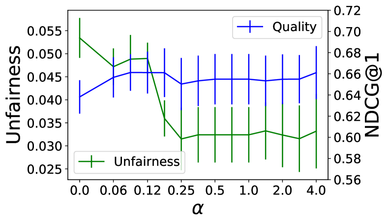
(a) Demographic parity, TREC data

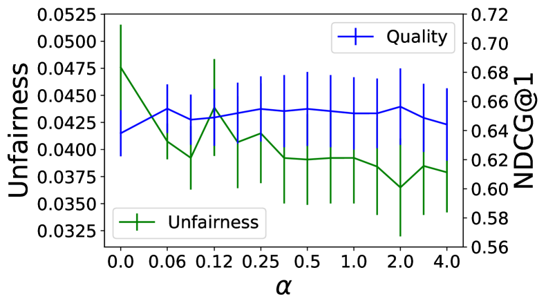
(b) Equalized odds, TREC data

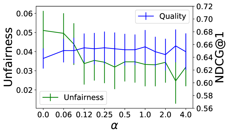
(c) Equality of opportunity, TREC data

Figure 5: $k=1,t=3$

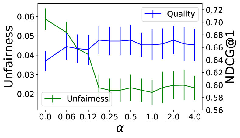
(a) Demographic parity, TREC data

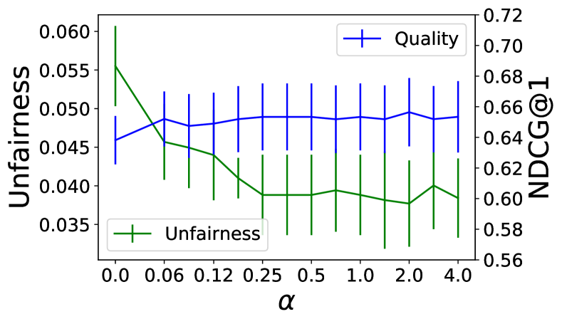
(b) Equalized odds, TREC data

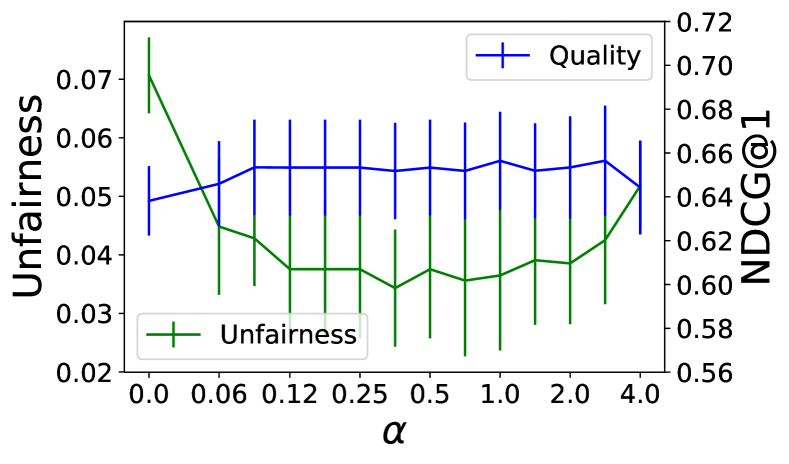
(c) Equality of opportunity, TREC data

Figure 6: $k=1,t=4$

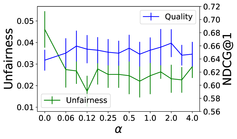
(a) Demographic parity, TREC data

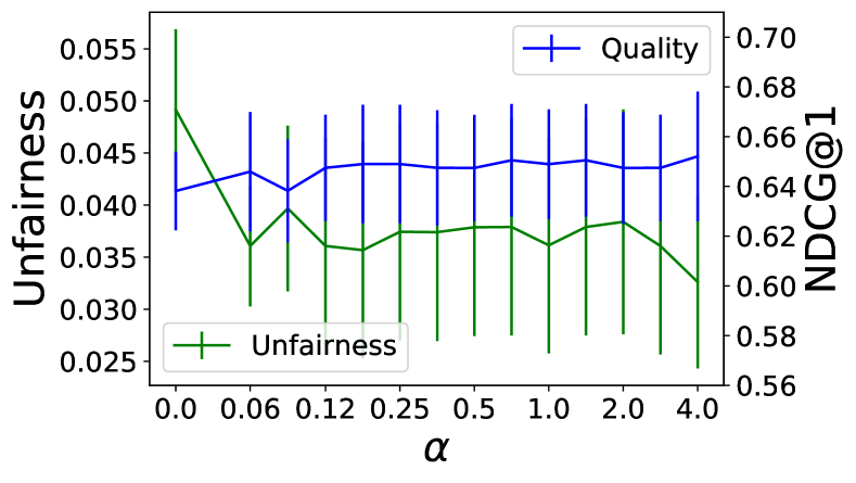
(b) Equalized odds, TREC data

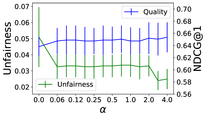
(c) Equality of opportunity, TREC data

Figure 7: $k=1,t=5$

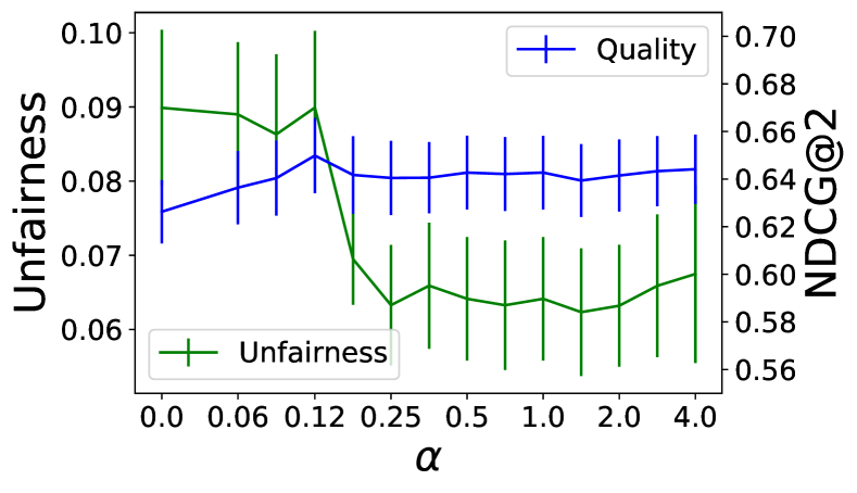
(a) Demographic parity, TREC data

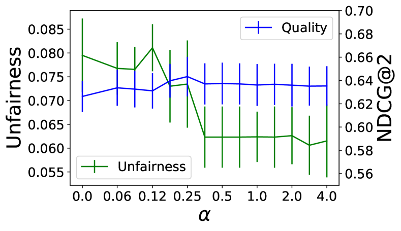
(b) Equalized odds, TREC data

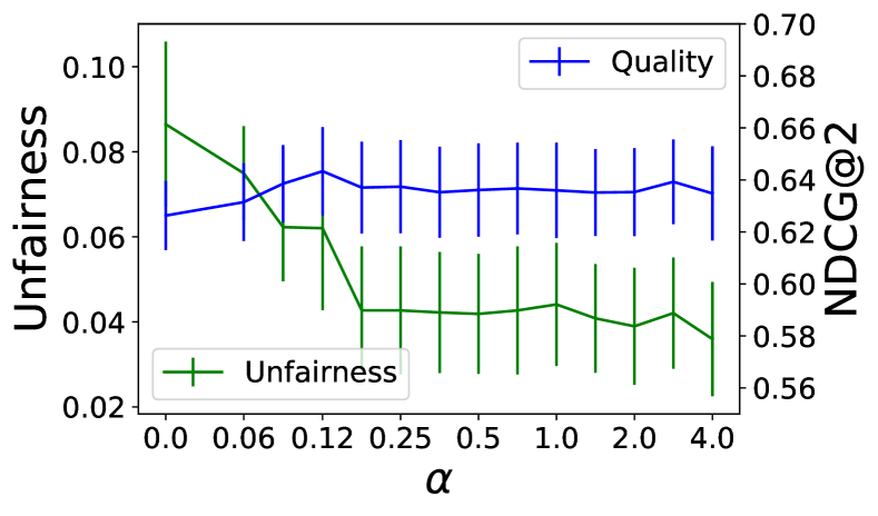
(c) Equality of opportunity, TREC data

Figure 8: $k=2,t=3$

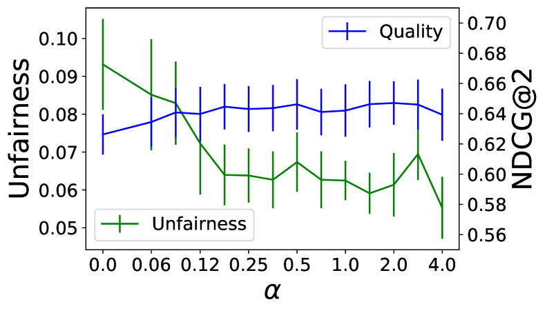
(a) Demographic parity, TREC data

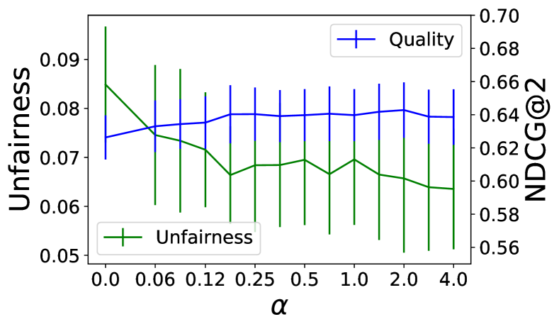
(b) Equalized odds, TREC data

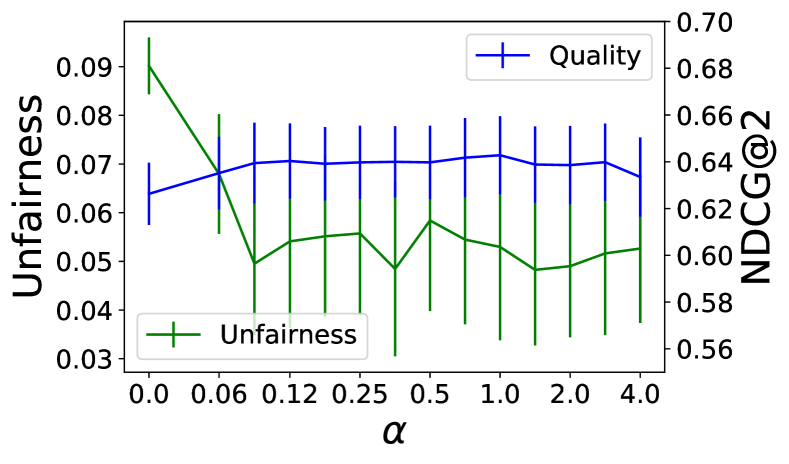
(c) Equality of opportunity, TREC data

Figure 9: $k=2,t=4$

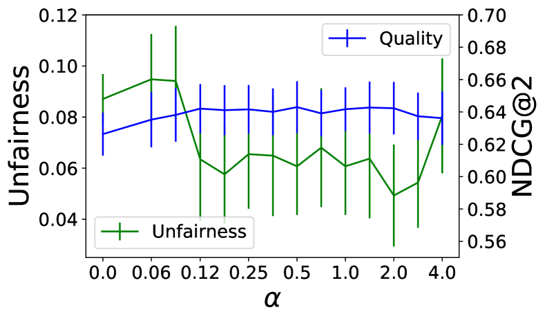
(a) Demographic parity, TREC data

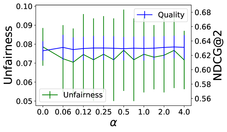
(b) Equalized odds, TREC data

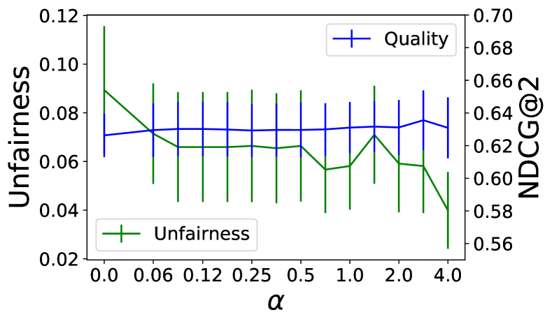
(c) Equality of opportunity, TREC data

Figure 10: $k=2,t=5$

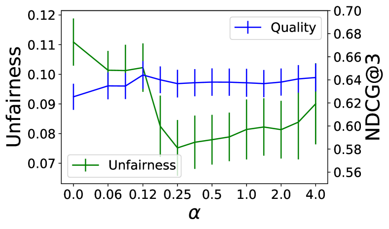
(a) Demographic parity, TREC data

(b) Equalized odds, TREC data

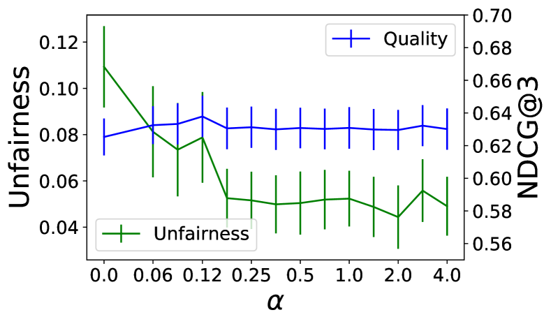
(c) Equality of opportunity, TREC data

Figure 11: $k=3,t=3$

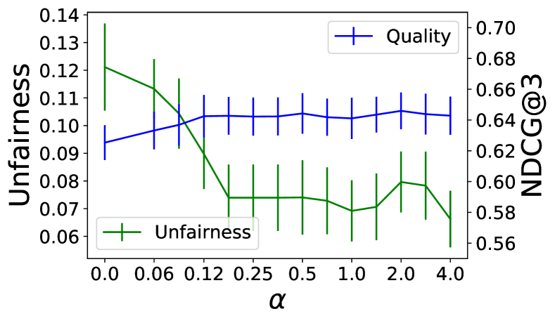
(a) Demographic parity, TREC data

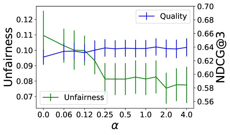
(b) Equalized odds, TREC data

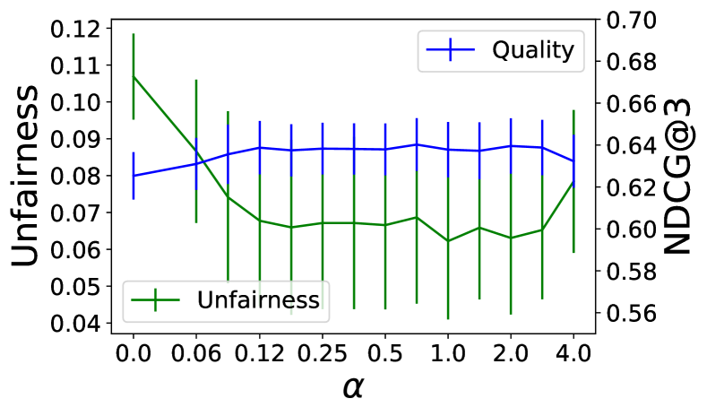
(c) Equality of opportunity, TREC data

Figure 12: $k=3,t=4$

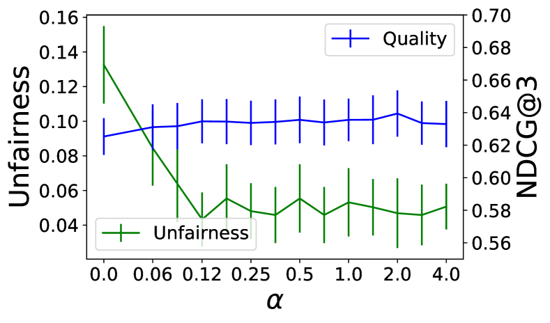
(a) Demographic parity, TREC data

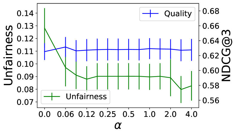
(b) Equalized odds, TREC data

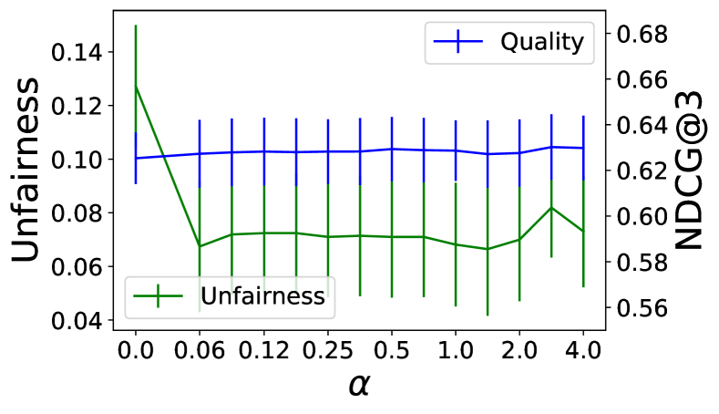
(c) Equality of opportunity, TREC data

Figure 13: $k=3,t=5$

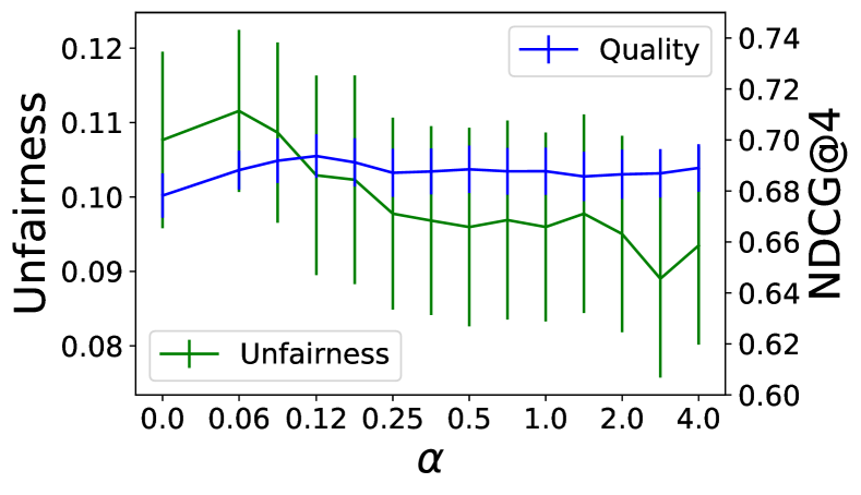
(a) Demographic parity, TREC data

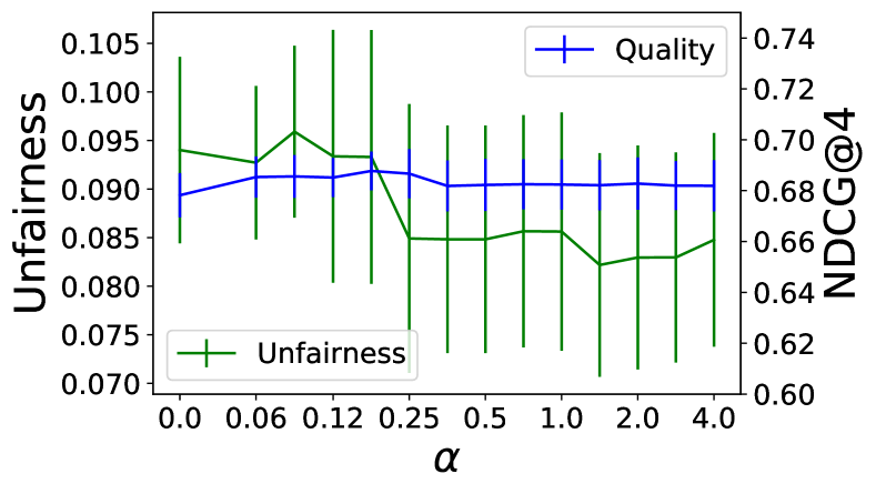
(b) Equalized odds, TREC data

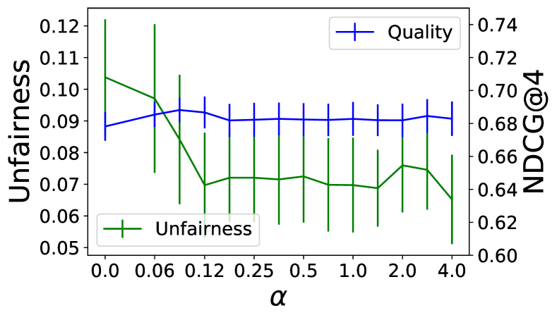
(c) Equality of opportunity, TREC data

Figure 14: $k=4,t=3$

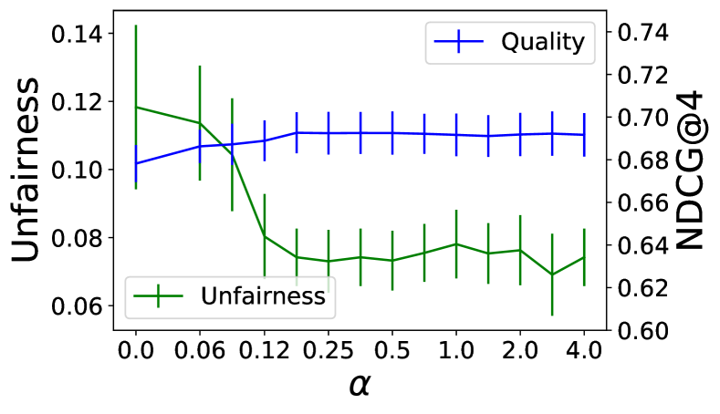
(a) Demographic parity, TREC data

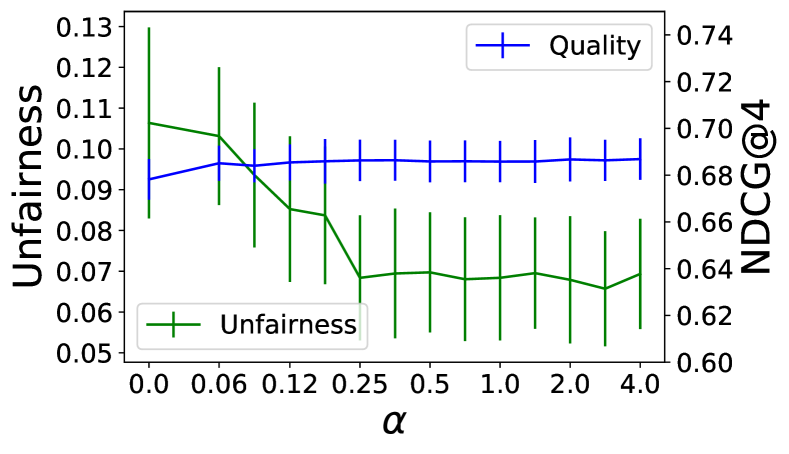
(b) Equalized odds, TREC data

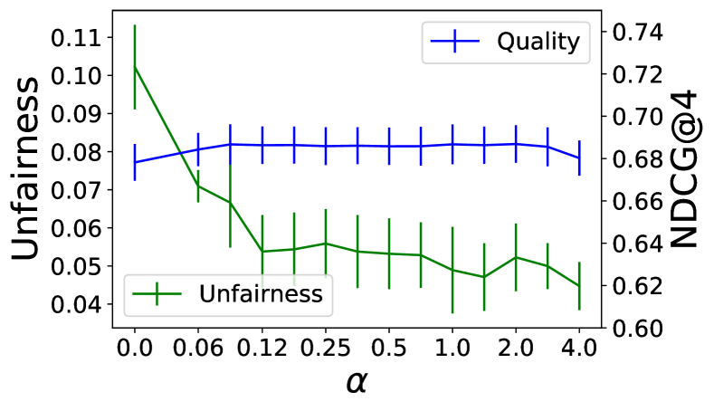
(c) Equality of opportunity, TREC data

Figure 15: $k=4,t=4$

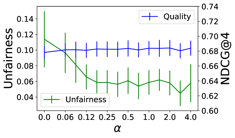
(a) Demographic parity, TREC data

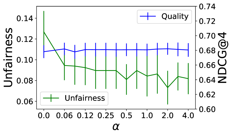
(b) Equalized odds, TREC data

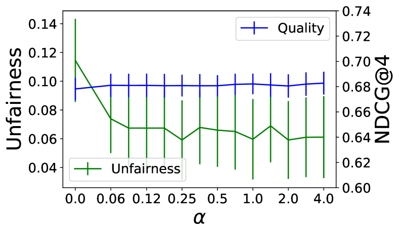
(c) Equality of opportunity, TREC data

Figure 16: $k=4,t=5$

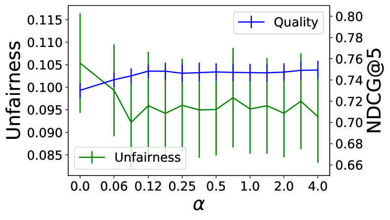
(a) Demographic parity, TREC data

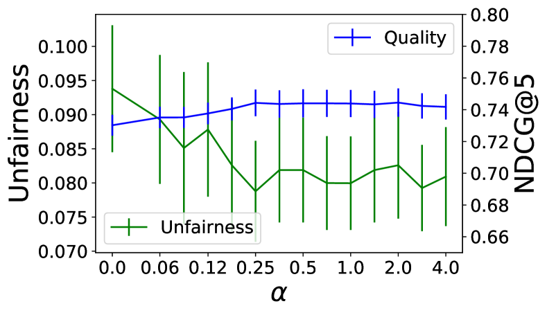
(b) Equalized odds, TREC data

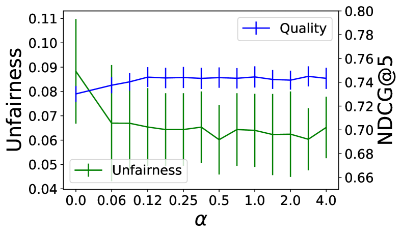
(c) Equality of opportunity, TREC data

Figure 17: $k=5,t=3$

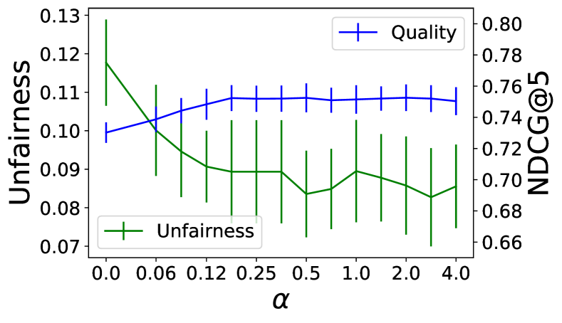
(a) Demographic parity, TREC data

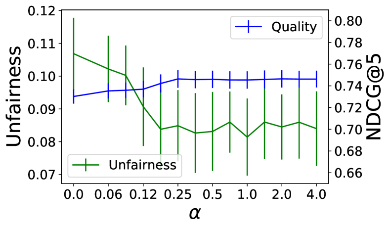
(b) Equalized odds, TREC data

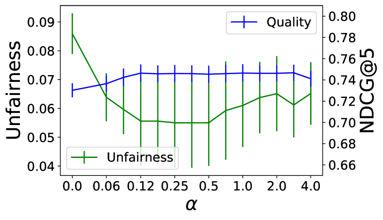
(c) Equality of opportunity, TREC data

Figure 18: $k=5,t=4$

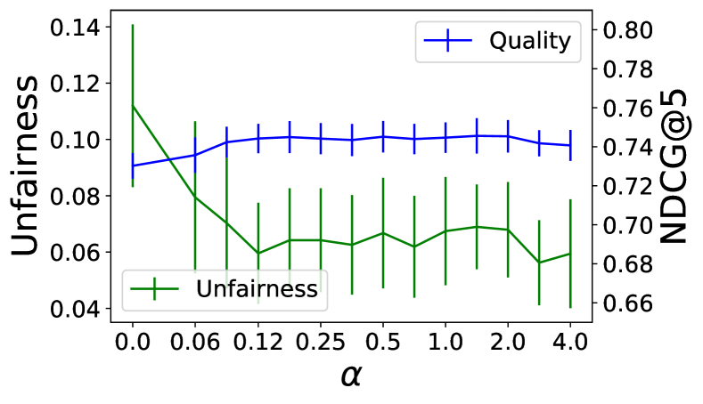
(a) Demographic parity, TREC data

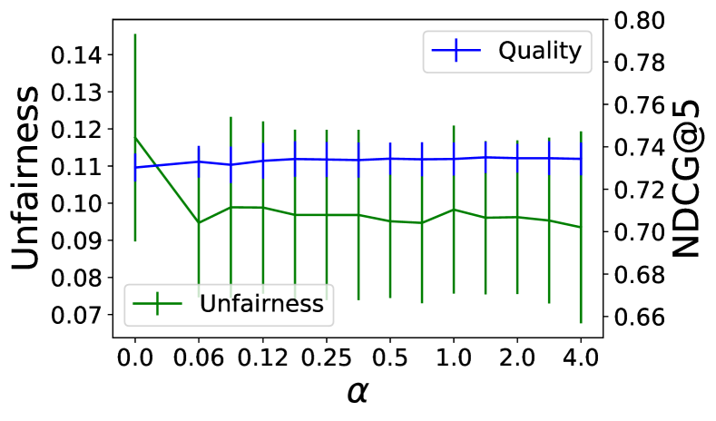
(b) Equalized odds, TREC data

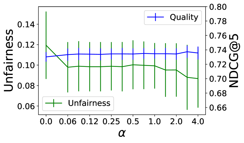
(c) Equality of opportunity, TREC data

Figure 19: $k=5,t=5$

C.4.2 MSMARCO results

Different rows correspond to different values of $k$ and the two different splits into protected groups (com and ext).

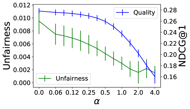
(a) Demographic parity, MSMARCO

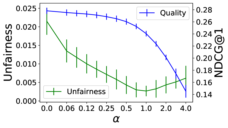
(b) Equalized odds, MSMARCO

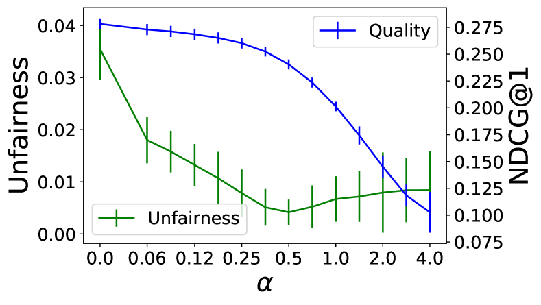
(c) Equality of opportunity, MSMARCO

Figure 20: $k=1$, com

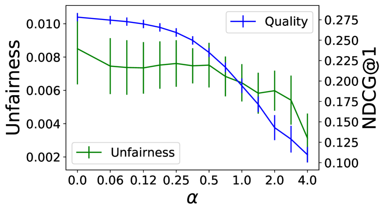
(a) Demographic parity, MSMARCO

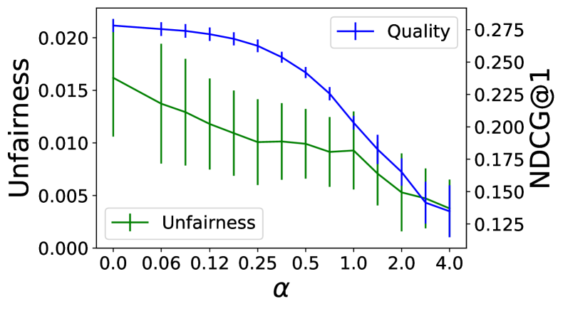
(b) Equalized odds, MSMARCO

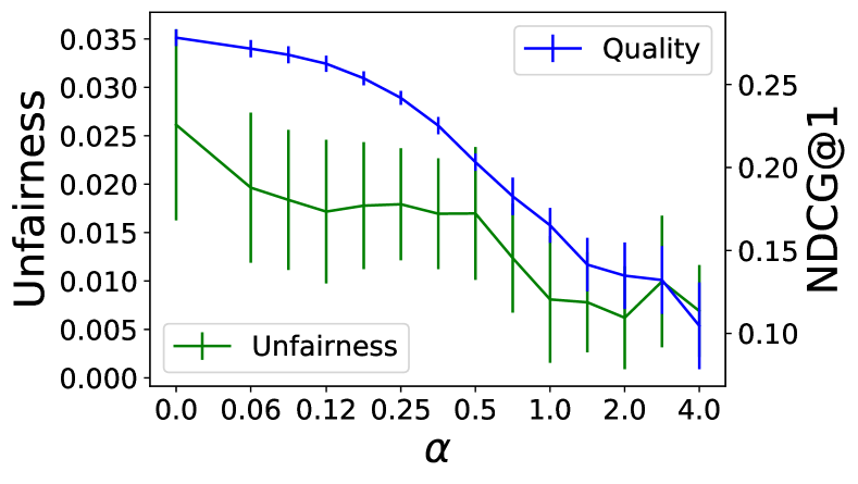
(c) Equality of opportunity, MSMARCO

Figure 21: $k=1$, ext

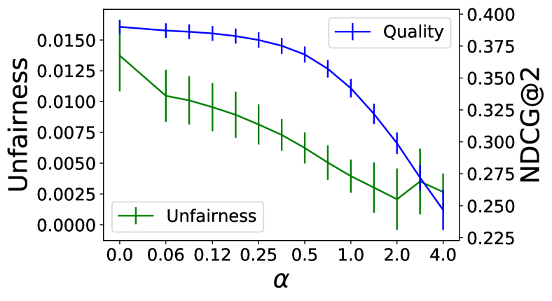
(a) Demographic parity, MSMARCO

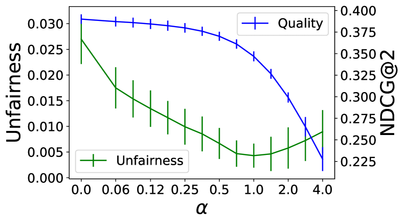
(b) Equalized odds, MSMARCO

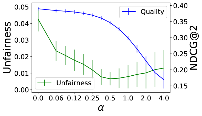
(c) Equality of opportunity, MSMARCO

Figure 22: $k=2$, com

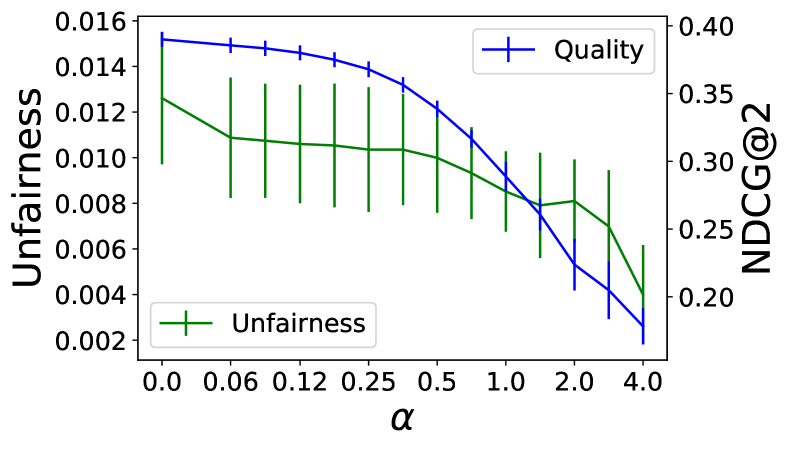
(a) Demographic parity, MSMARCO

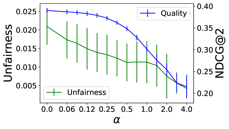
(b) Equalized odds, MSMARCO

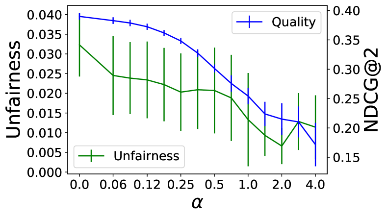
(c) Equality of opportunity, MSMARCO

Figure 23: $k=2$, ext

(a) Demographic parity, MSMARCO

(b) Equalized odds, MSMARCO

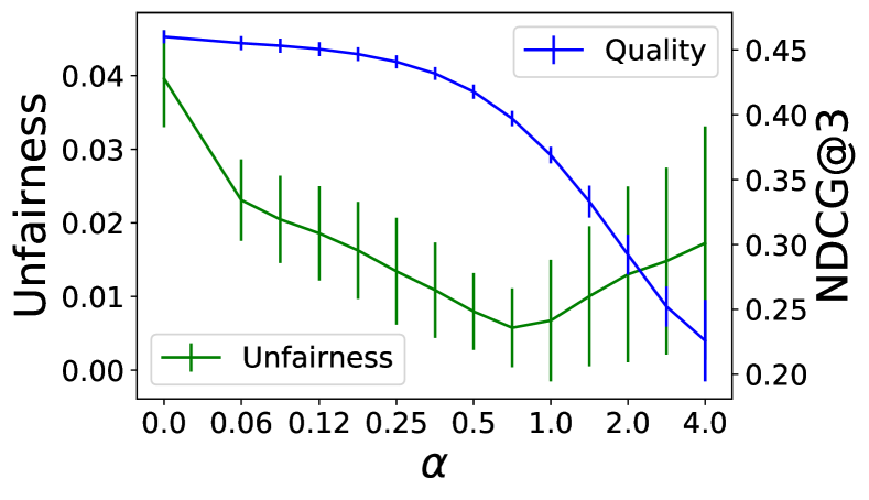
(c) Equality of opportunity, MSMARCO

Figure 24: $k=3$, com

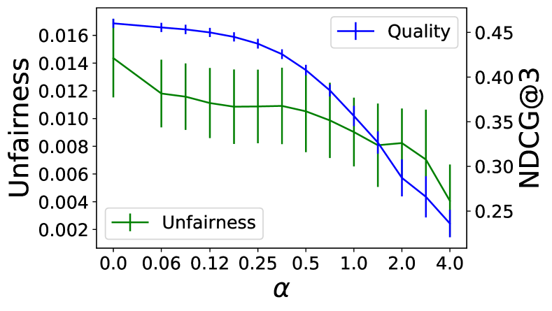
(a) Demographic parity, MSMARCO

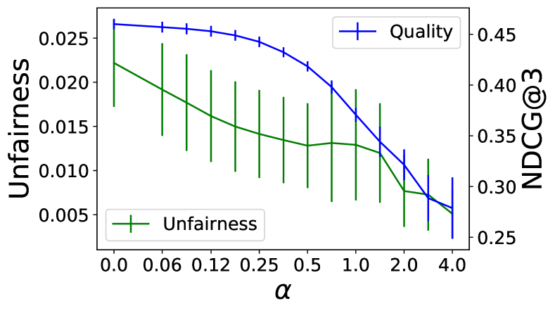
(b) Equalized odds, MSMARCO

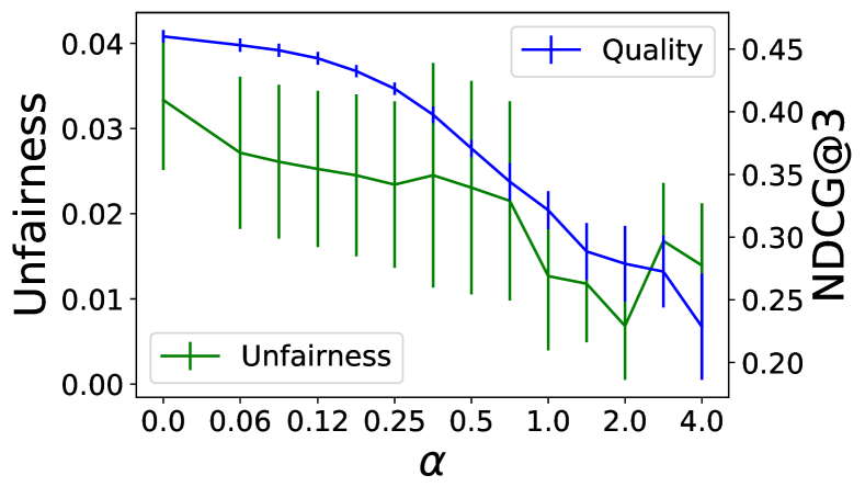
(c) Equality of opportunity, MSMARCO

Figure 25: $k=3$, ext

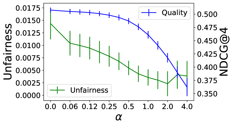
(a) Demographic parity, MSMARCO

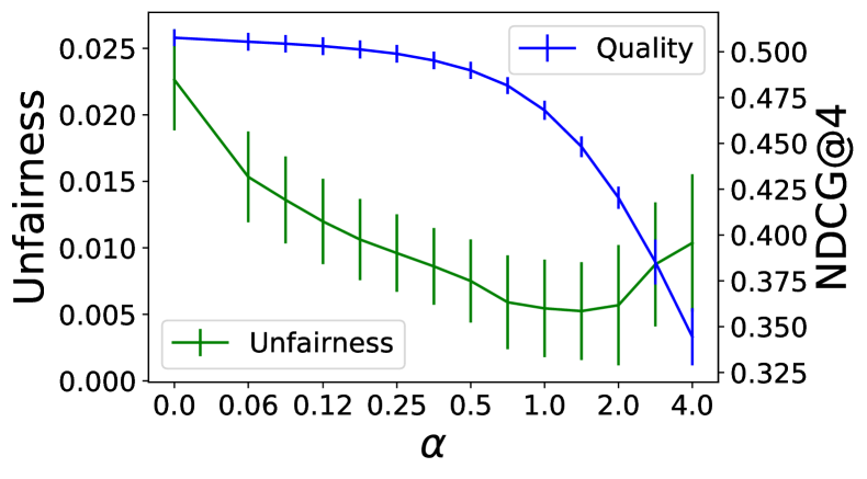
(b) Equalized odds, MSMARCO

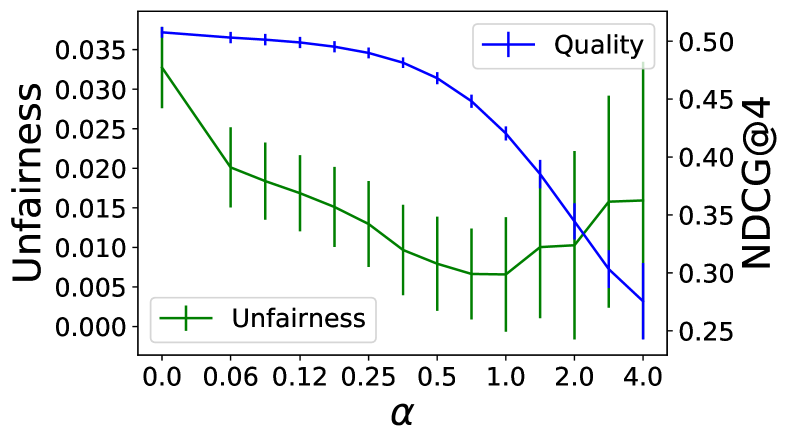
(c) Equality of opportunity, MSMARCO

Figure 26: $k=4$, com

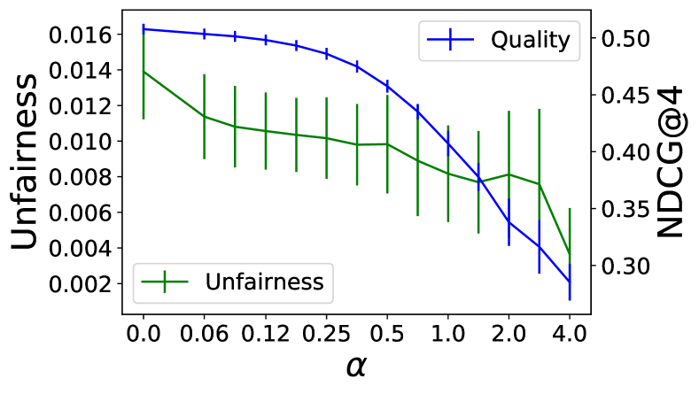
(a) Demographic parity, MSMARCO

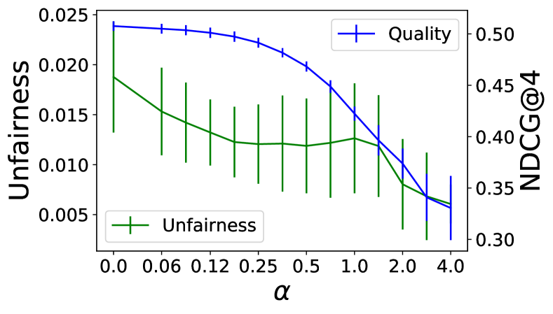
(b) Equalized odds, MSMARCO

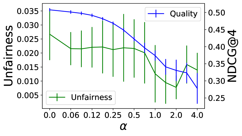
(c) Equality of opportunity, MSMARCO

Figure 27: $k=4$, ext

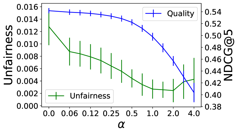
(a) Demographic parity, MSMARCO

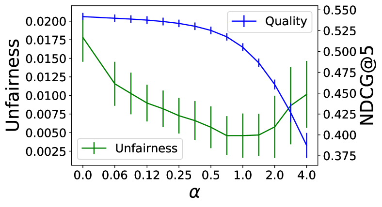
(b) Equalized odds, MSMARCO

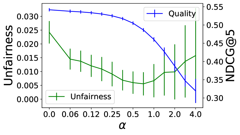
(c) Equality of opportunity, MSMARCO

Figure 28: $k=5$, com

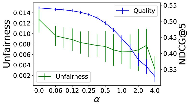
(a) Demographic parity, MSMARCO

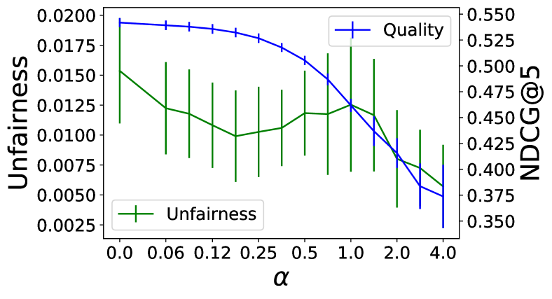
(b) Equalized odds, MSMARCO

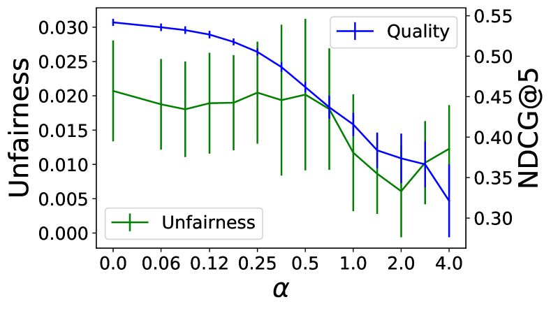
(c) Equality of opportunity, MSMARCO

Figure 29: $k=5$, ext

References

- Abadi et al. [2015] M. Abadi, A. Agarwal, P. Barham, E. Brevdo, Z. Chen, C. Citro, G. S. Corrado, A. Davis, J. Dean, M. Devin, S. Ghemawat, I. Goodfellow, A. Harp, G. Irving, M. Isard, Y. Jia, R. Jozefowicz, L. Kaiser, M. Kudlur, J. Levenberg, D. Mané, R. Monga, S. Moore, D. Murray, C. Olah, M. Schuster, J. Shlens, B. Steiner, I. Sutskever, K. Talwar, P. Tucker, V. Vanhoucke, V. Vasudevan, F. Viégas, O. Vinyals, P. Warden, M. Wattenberg, M. Wicke, Y. Yu, and X. Zheng. TensorFlow: Large-scale machine learning on heterogeneous systems, 2015. URL https://www.tensorflow.org/. Software available from tensorflow.org.
- Agarwal et al. [2018] A. Agarwal, A. Beygelzimer, M. Dudík, J. Langford, and H. Wallach. A reductions approach to fair classification. In International Conference on Machine Learing (ICML), 2018.
- Asudeh et al. [2019] A. Asudeh, H. Jagadish, J. Stoyanovich, and G. Das. Designing fair ranking schemes. In International Conference on Management of Data (COMAD), 2019.
- Baharlouei et al. [2019] S. Baharlouei, M. Nouiehed, A. Beirami, and M. Razaviyayn. Rényi fair inference. In International Conference on Learning Representations (ICLR), 2019.
- Barocas et al. [2019] S. Barocas, M. Hardt, and A. Narayanan. Fairness and Machine Learning. 2019. http://www.fairmlbook.org.
- Bartlett and Mendelson [2002] P. L. Bartlett and S. Mendelson. Rademacher and gaussian complexities: Risk bounds and structural results. Journal of Machine Learning Research (JMLR), 2002.
- Bengio et al. [2019] S. Bengio, K. Dembczynski, T. Joachims, M. Kloft, and M. Varma. Extreme classification. In Dagstuhl Reports 18291. Schloss Dagstuhl – Leibniz Center for Informatics, 2019.
- Beutel et al. [2019] A. Beutel, J. Chen, T. Doshi, H. Qian, L. Wei, Y. Wu, L. Heldt, Z. Zhao, L. Hong, E. H. Chi, et al. Fairness in recommendation ranking through pairwise comparisons. In Conference on Knowledge Discovery and Data Mining (KDD), 2019.
- Biddle [2006] D. Biddle. Adverse impact and test validation: A practitioner’s guide to valid and defensible employment testing. Gower Publishing, 2006.
- Biega et al. [2018] A. J. Biega, K. P. Gummadi, and G. Weikum. Equity of attention: Amortizing individual fairness in rankings. In International Conference on Research and Development in Information Retrieval (SIGIR), 2018.
- Biega et al. [2019] A. J. Biega, F. Diaz, M. D. Ekstrand, and S. Kohlmeier. Overview of the TREC 2019 fair ranking track. In The Twenty-Eighth Text REtrieval Conference (TREC 2019) Proceedings, 2019.
- Bonart [2019] M. Bonart. Fair ranking in academic search, 2019. URL https://trec.nist.gov/pubs/trec28/papers/IR-Cologne.FR.pdf.
- Bower et al. [2021] A. Bower, H. Eftekhari, M. Yurochkin, and Y. Sun. Individually fair rankings. In International Conference on Learning Representations (ICLR), 2021.
- Burke [2017] R. Burke. Multisided fairness for recommendation. arXiv preprint arXiv:1707.00093, 2017.
- Burke et al. [2018] R. Burke, N. Sonboli, and A. Ordonez-Gauger. Balanced neighborhoods for multi-sided fairness in recommendation. In Conference on Fairness, Accountability and Transparency (FAccT), 2018.
- Calders and Verwer [2010] T. Calders and S. Verwer. Three naive Bayes approaches for discrimination-free classification. Data Mining and Knowledge Discovery (DMKD), 2010.
- Calders et al. [2009] T. Calders, F. Kamiran, and M. Pechenizkiy. Building classifiers with independency constraints. In International Conference on Data Mining Workshops (IDCMW), 2009.
- Castillo [2019] C. Castillo. Fairness and transparency in ranking. In International Conference on Research and Development in Information Retrieval (SIGIR), 2019.
- Celis et al. [2018] L. E. Celis, D. Straszak, and N. K. Vishnoi. Ranking with fairness constraints. In International Colloquium on Automata, Languages, and Programming (ICALP). Schloss Dagstuhl – Leibniz Center for Informatics, 2018.
- Celis et al. [2020] L. E. Celis, A. Mehrotra, and N. K. Vishnoi. Interventions for ranking in the presence of implicit bias. In Conference on Fairness, Accountability and Transparency (FAccT), 2020.
- Chakraborty et al. [2019] A. Chakraborty, G. K. Patro, N. Ganguly, K. P. Gummadi, and P. Loiseau. Equality of voice: Towards fair representation in crowdsourced top-k recommendations. In Conference on Fairness, Accountability and Transparency (FAccT), 2019.
- Cho et al. [2020] J. Cho, G. Hwang, and C. Suh. A fair classifier using kernel density estimation. Conference on Neural Information Processing Systems (NeurIPS), 2020.
- Cotter et al. [2019] A. Cotter, M. Gupta, H. Jiang, N. Srebro, K. Sridharan, S. Wang, B. Woodworth, and S. You. Training well-generalizing classifiers for fairness metrics and other data-dependent constraints. In International Conference on Machine Learing (ICML), 2019.
- Devlin et al. [2019] J. Devlin, M.-W. Chang, K. Lee, and K. Toutanova. BERT: Pre-training of deep bidirectional transformers for language understanding. In Annual Meeting of the Association for Computational Linguistics (ACL), 2019.
- Dwork et al. [2012] C. Dwork, M. Hardt, T. Pitassi, O. Reingold, and R. Zemel. Fairness through awareness. In Innovations in Theoretical Computer Science Conference (ITCS), 2012.
- Farnadi et al. [2018] G. Farnadi, P. Kouki, S. K. Thompson, S. Srinivasan, and L. Getoor. A fairness-aware hybrid recommender system. arXiv preprint arXiv:1809.09030, 2018.
- Geyik et al. [2019] S. C. Geyik, S. Ambler, and K. Kenthapadi. Fairness-aware ranking in search & recommendation systems with application to linkedin talent search. In Conference on Knowledge Discovery and Data Mining (KDD), 2019.
- Gorantla et al. [2020] S. Gorantla, A. Deshpande, and A. Louis. Ranking for individual and group fairness simultaneously. arXiv preprint arXiv:2010.06986, 2020.
- Han et al. [2020] S. Han, X. Wang, M. Bendersky, and M. Najork. Learning-to-rank with BERT in TF-ranking. arXiv preprint arXiv:2004.08476, 2020.
- Hardt et al. [2016] M. Hardt, E. Price, and N. Srebro. Equality of opportunity in supervised learning. In Conference on Neural Information Processing Systems (NeurIPS), 2016.
- Janson [2004] S. Janson. Large deviations for sums of partly dependent random variables. Random Structures & Algorithms, 24(3):234–248, 2004.
- Joachims [2002] T. Joachims. Optimizing search engines using clickthrough data. In Conference on Knowledge Discovery and Data Mining (KDD), 2002.
- Kallus and Zhou [2019] N. Kallus and A. Zhou. The fairness of risk scores beyond classification: Bipartite ranking and the xAUC metric. In Conference on Neural Information Processing Systems (NeurIPS), 2019.
- Kamishima et al. [2011] T. Kamishima, S. Akaho, and J. Sakuma. Fairness-aware learning through regularization approach. In 11th International Conference on Data Mining Workshops, 2011.
- Kamishima et al. [2012a] T. Kamishima, S. Akaho, H. Asoh, and J. Sakuma. Enhancement of the neutrality in recommendation. In Decisions@ RecSys, 2012a.
- Kamishima et al. [2012b] T. Kamishima, S. Akaho, H. Asoh, and J. Sakuma. Fairness-aware classifier with prejudice remover regularizer. In European Conference on Machine Learning and Data Mining (ECML PKDD), 2012b.
- Kamishima et al. [2014] T. Kamishima, S. Akaho, H. Asoh, and J. Sakuma. Correcting popularity bias by enhancing recommendation neutrality. In RecSys Posters, 2014.
- Kim et al. [2020] J. S. Kim, J. Chen, and A. Talwalkar. Fact: A diagnostic for group fairness trade-offs. In International Conference on Machine Learing (ICML), 2020.
- Kuhlman et al. [2019] C. Kuhlman, M. VanValkenburg, and E. Rundensteiner. FARE: Diagnostics for fair ranking using pairwise error metrics. In International World Wide Web Conference (WWW), 2019.
- Kusner et al. [2017] M. J. Kusner, J. Loftus, C. Russell, and R. Silva. Counterfactual fairness. In Conference on Neural Information Processing Systems (NeurIPS), 2017.
- Liu [2011] T.-Y. Liu. Learning to rank for information retrieval. Springer Science & Business Media, 2011.
- Lo [2015] D. Lo. When you Google image CEO, the first female photo on the results page is Barbie. https://www.glamour.com/story/google-search-ceo, 2015. Accessed: 2021-05-26.
- Manning et al. [2008] C. D. Manning, H. Schütze, and P. Raghavan. Introduction to information retrieval. Cambridge University Press, 2008.
- Mehrabi et al. [2019] N. Mehrabi, F. Morstatter, N. Saxena, K. Lerman, and A. Galstyan. A survey on bias and fairness in machine learning. arXiv preprint arXiv:1908.09635, 2019.
- Mitra and Craswell [2018] B. Mitra and N. Craswell. An introduction to neural information retrieval. Foundations and Trends in Information Retrieval, 2018.
- Morik et al. [2020] M. Morik, A. Singh, J. Hong, and T. Joachims. Controlling fairness and bias in dynamic learning-to-rank. In International Conference on Research and Development in Information Retrieval (SIGIR), 2020.
- Narasimhan et al. [2020] H. Narasimhan, A. Cotter, M. R. Gupta, and S. Wang. Pairwise fairness for ranking and regression. In Conference on Artificial Intelligence (AAAI), 2020.
- Nguyen et al. [2016] T. Nguyen, M. Rosenberg, X. Song, J. Gao, S. Tiwary, R. Majumder, and L. Deng. MS MARCO: A human-generated machine reading comprehension dataset. In Conference on Neural Information Processing Systems (NeurIPS), 2016.
- Nogueira and Cho [2019] R. Nogueira and K. Cho. Passage re-ranking with BERT. arXiv preprint arXiv:1901.04085, 2019.
- Peysakhovich and Kroer [2019] A. Peysakhovich and C. Kroer. Fair division without disparate impact. arXiv preprint arXiv:1906.02775, 2019.
- Radlinski et al. [2009] F. Radlinski, P. N. Bennett, B. Carterette, and T. Joachims. Redundancy, diversity and interdependent document relevance. In International Conference on Research and Development in Information Retrieval (SIGIR), 2009.
- Rezaei et al. [2020] A. Rezaei, R. Fathony, O. Memarrast, and B. Ziebart. Fairness for robust log loss classification. In Conference on Artificial Intelligence (AAAI), 2020.
- Robertson [1977] S. E. Robertson. The probability ranking principle in ir. Journal of Documentation, 33(4):294–304, 1977.
- Sapiezynski et al. [2019] P. Sapiezynski, W. Zeng, R. E Robertson, A. Mislove, and C. Wilson. Quantifying the impact of user attentionon fair group representation in ranked lists. In International World Wide Web Conference (WWW), 2019.
- Singh and Joachims [2017] A. Singh and T. Joachims. Equality of opportunity in rankings. In Workshop on Prioritizing Online Content (WPOC) at NeurIPS, 2017.
- Singh and Joachims [2018] A. Singh and T. Joachims. Fairness of exposure in rankings. In Conference on Knowledge Discovery and Data Mining (KDD), 2018.
- Singh and Joachims [2019] A. Singh and T. Joachims. Policy learning for fairness in ranking. In Conference on Neural Information Processing Systems (NeurIPS), 2019.
- Steck [2018] H. Steck. Calibrated recommendations. In Conference on Recommender Systems (RecSys), 2018.
- Tabibian et al. [2020] B. Tabibian, V. Gómez, A. De, B. Schölkopf, and M. G. Rodriguez. On the design of consequential ranking algorithms. In Uncertainty in Artificial Intelligence (UAI), 2020.
- Tan et al. [2020] Z. Tan, S. Yeom, M. Fredrikson, and A. Talwalkar. Learning fair representations for kernel models. In Conference on Uncertainty in Artificial Intelligence (AISTATS), 2020.
- Tsintzou et al. [2019] V. Tsintzou, E. Pitoura, and P. Tsaparas. Bias disparity in recommendation systems. In Workshop on Recommendation in Multi-stakeholder Environments at RecSys, 2019.
- Usunier et al. [2005] N. Usunier, M. R. Amini, and P. Gallinari. Generalization error bounds for classifiers trained with interdependent data. Conference on Neural Information Processing Systems (NeurIPS), 2005.
- Vapnik [2013] V. Vapnik. The nature of statistical learning theory. Springer, 2013.
- Vogel et al. [2020] R. Vogel, A. Bellet, and S. Clémençon. Learning fair scoring functions: Fairness definitions, algorithms and generalization bounds for bipartite ranking. arXiv preprint arXiv:2002.08159, 2020.
- Weston et al. [2011] J. Weston, S. Bengio, and N. Usunier. WSABIE: Scaling up to large vocabulary image annotation. In International Joint Conference on Artificial Intelligence (IJCAI), 2011.
- Wick et al. [2019] M. Wick, S. Panda, and J.-B. Tristan. Unlocking fairness: a trade-off revisited. In Conference on Neural Information Processing Systems (NeurIPS), 2019.
- Williamson and Menon [2019] R. Williamson and A. Menon. Fairness risk measures. In International Conference on Machine Learing (ICML), 2019.
- Woodworth et al. [2017] B. Woodworth, S. Gunasekar, M. I. Ohannessian, and N. Srebro. Learning non-discriminatory predictors. In Workshop on Computational Learning Theory (COLT), 2017.
- Wu et al. [2018] Y. Wu, L. Zhang, and X. Wu. On discrimination discovery and removal in ranked data using causal graph. In Conference on Knowledge Discovery and Data Mining (KDD), 2018.
- Yadav et al. [2019] H. Yadav, Z. Du, and T. Joachims. Fair learning-to-rank from implicit feedback. arXiv preprint arXiv:1911.08054, 2019.
- Yang and Stoyanovich [2017] K. Yang and J. Stoyanovich. Measuring fairness in ranked outputs. In Scientific and Statistical Database Management Conference (SSDBM), 2017.
- Yang et al. [2019] K. Yang, V. Gkatzelis, and J. Stoyanovich. Balanced ranking with diversity constraints. In International Joint Conference on Artificial Intelligence (IJCAI), 2019.
- Zafar et al. [2017] M. B. Zafar, I. Valera, M. G. Rogriguez, and K. P. Gummadi. Fairness constraints: Mechanisms for fair classification. In Conference on Uncertainty in Artificial Intelligence (AISTATS), 2017.
- Zehlike and Castillo [2020] M. Zehlike and C. Castillo. Reducing disparate exposure in ranking: A learning to rank approach. In International World Wide Web Conference (WWW), 2020.
- Zehlike et al. [2017] M. Zehlike, F. Bonchi, C. Castillo, S. Hajian, M. Megahed, and R. Baeza-Yates. FA*IR: A fair top-k ranking algorithm. In Conference on Information and Knowledge Management (CIKM), 2017.
- Zehlike et al. [2020] M. Zehlike, T. Sühr, C. Castillo, and I. Kitanovski. Fairsearch: A tool for fairness in ranked search results. In International World Wide Web Conference (WWW), 2020.
- Zhang et al. [2018] B. H. Zhang, B. Lemoine, and M. Mitchell. Mitigating unwanted biases with adversarial learning. In Proceedings of the 2018 AAAI/ACM Conference on AI, Ethics, and Society, 2018.
- Zhu et al. [2018] Z. Zhu, X. Hu, and J. Caverlee. Fairness-aware tensor-based recommendation. In Conference on Information and Knowledge Management (CIKM), 2018.