Vorticity Production at Fluid Interfaces in Two-dimensional Flows

Abstract

This work revisits the production of vorticity at an interface separating two immiscible incompressible fluids. A new decomposition of the vorticity flux is proposed in a two-dimensional context which allows to compute explicitly such a quantity in terms of surface tension $\sigma$, viscosity $\mu$ and gravity $g$. This approach is then applied in the context of gravito-capillary waves. It leads to analytical results already known but from a new perspective, provides some quantitative predictions at short time that can be a good test for numerical codes. Finally it is a mean to obtain a qualitative understanding of direct numerical simulation results.

1 Introduction

When fluid properties such as density are varying in a spatial domain, vorticity is generated in that domain by a baroclinic effect ¹⁵. If this region is an extremely thin layer, it is considered from the view point of continuum mechanics to be a sharp discontinuity between two fluids. As a consequence, fluid/fluid interface plays the role of a source of vorticity as for a fluid/solid interfaces. Contrary to the fluid/solid interface, the produced vorticity eventually influences the dynamical response of the interface itself. This manuscript discusses and quantifies the generation of vorticity produced at the interface between two incompressible and immiscible fluids within the context of two-dimensional flows.

Initial theoretical works on vorticity field at interfaces were devoted to the particular case of a free surface flow, imposing zero shear stress at the interface and a constant pressure in the outer fluid due to the neglect of the outer fluid dynamical viscosity and density. Various papers ^{9; 10} obtained in a steady two dimensional flow, (see also ¹), the relation $\omega=-2\kappa~{}(\vec{u}\cdot\vec{t})$ giving vorticity at free boundary $\omega$ as a function of interface curvature $\kappa$ and tangential velocity $\vec{u}\cdot\vec{t}$. This result and its generalization to three-dimensions ¹¹; ¹⁶, stress the intrinsic relation between interface topology and vorticity intensity. Furthermore the presence of thin vorticity layers at the interface have motivated the development of theoretical and numerical methods based on the boundary-layer approach where the potential flow far from the surface is constrained by the conditions imposed by an infinitely thin boundary layer at the interface. These models have successfully reproduced the response of weakly damped Stokes waves ¹⁰ and obtained constraints in the relation between flow properties and vorticity field at the interface in two-dimensional steady flows imposed by the stress free condition ²¹.

The relation $\omega=-2\kappa~{}(\vec{u}\cdot\vec{t})$ is based on a kinematical relationship plus the definition of zero shear but does not depend on the condition imposed on pressure at the interface. This is related to the fact that, vorticity produced at the surface diffuses into the bulk ⁹; ⁸ although this process is not given by the previous relation. More precisely, the value of vorticity imposed at the free surface does not provide the rate at which vorticity diffuses into the bulk that ultimately is the vorticity production rate. For example while the vorticity along a steady flat surface is null, the vorticity production and the diffusion of vorticity towards the interface is found to be proportional to the pressure gradient along the surface and therefore not necessarily null in this particular case ¹². Thus, following the work of Lighthill ⁷ where a vorticity sheet along the interface is introduced to satisfy the non-slip boundary condition in a fluid/solid interface, various authors have focused their efforts to derive generalized expressions for the vorticity generation at a free surface in non-steady flows equations ²⁰; ¹⁴.

The initial works on the production of vorticity by interfaces in free surface flows have been extended to interfaces between two immiscible fluids with arbitrary values of density and viscosity allowing to study the influence of vorticity production beyond the limiting case of free surface flows. Lugt ¹² already discusses some constrains imposed in the angle between streamlines at the surface between two viscous fluids. The dynamic viscosity ratio was identified to be the parameter controling the streamline patterns for steady two-dimensional incompressible flows. Later, ^{26; 25} expressed the production of vorticity by sharp interfaces between two viscous fluids and ⁴ establishes the relations that must be used in vorticity-based formulations for the interface between two viscous fluids providing also an evolution equation for the vortex sheet-strength. More recently ^{3; 2} and ²³ have extended the work of ¹⁴ to obtain general expressions for the production of vorticity by fluid/fluid interfaces in two–dimensional flows for both non-slip and stress-free conditions discussing the consequences of vorticity generation in various problems involving the presence of interfaces between two viscous fluids.

In the present paper, we revise the previous expressions of the vorticity production in two–dimensions. First we provide a symmetric expression for the sources of vorticity. Second and more importantly, we derive the explicit dependency of the vorticity production with respect to surface tension, viscosity and gravity. Thereafter we apply this approach to the problem of gravity–capillary waves widely studied in the literature for both linear ⁶; ¹⁹ and non-linear regimes ¹³; ⁵. It is shown that this formulation is useful to understand the transition between the linear and non-linear regime and explain the symmetry breaking of oscillations of gravity waves.

The manuscript is structured as follows. Section 2 recalls some previous theoretical results about vorticity production at an interface. Section 3 introduces a new decomposition of the production term in terms of pressure jump and mean pressure at interface. The procedure to compute the mean pressure is then presented. The result of this approach is an explicit expression of vorticity production which discriminates the various mechanisms (section 4). In the end of this section some asymptotic cases are given. Such a theoretical result is then applied on the flow example of a gravito-capillary wave. For linear viscous waves, one recovers previously known analytical results in an alternative way (section  5). For the non-linear regime, cases of non-linear evolution are studied from this new viewpoint, providing some qualitative interpretations (section 6).

2 Vorticity production at interfaces.

This section recalls the main previous theoretical results and defines our notations. Let us consider a two-dimensional flow with two incompressible and immiscible fluids separated by an interface $(I)$ possessing a surface tension $\sigma$. Each fluid possesses a constant density $\rho^{(r)}$ or equivalently a specific volume $\upsilon^{(r)}\equiv{1}/{\rho^{(r)}}$, a constant dynamic viscosity $\mu^{(r)}$ or equivalently a kinematic viscosity $\nu^{(r)}\equiv\mu^{(r)}\upsilon^{(r)}$. In the plane $(x,y)$ oriented by the unit normal $\vec{e}_{z}$, interface position and velocity components $u_{i}(x,y,t),~{}~{}i=1,2$ provide a complete description of the flow (we use in some obvious occasions $x$ for $x_{1}$ and $y$ for $x_{2}$). This flow is governed by the Navier–Stokes equation

$$\rho^{(r)}\frac{D{u}_{i}^{(r)}}{Dt}=\partial_{j}\tau_{ij}^{(r)}+\rho^{(r)}F_{i}(\vec{x},t),~{}~{}~{}~{}~{}\partial_{i}u_{i}=0$$ (1)

where $D/Dt\equiv\partial/\partial t+{u}_{i}^{(r)}\partial_{i}$ denotes the Lagrangian time derivative and $\tau_{ij}^{(r)}$ the stress tensor

$$\tau^{(r)}_{ij}=-p^{(r)}\delta_{ij}+2\mu^{(r)}e^{(r)}_{ij},~{}~{}~{}~{}~{}~{}e^{(r)}_{ij}=\frac{1}{2}[\partial_{i}u^{(r)}_{j}+\partial_{j}u^{(r)}_{i}].$$ (2)

The force per unit mass $\vec{F}(\vec{x},t)$ is assumed to be continuous across the interface and to derive from a potential i.e. $\vec{F}=-\vec{\nabla}[g\varphi]$ where $g$ is an amplitude parameter. In the example studied below, $\vec{F}(\vec{x},t)$ is gravity : in that instance, coordinate $y$ stands for the upward vertical cartesian coordinate and $\varphi=y$ and $g=9.81$ the acceleration of gravity in S.I. units.

Vorticity field is directed along $\vec{e}_{z}$ and its unique component $\omega(x,y,t)$ is governed by

$$\frac{D\omega^{(r)}}{Dt}=-\nabla\cdot\vec{J}^{(r)},~{}~{}~{}\vec{J}^{(r)}\equiv-\nu^{(r)}\,\vec{\nabla}\omega^{(r)}$$ (3)

At any point of interface $(I)$, one attaches a Frenet–Serret frame. One may select the unit normal vector $\vec{n}^{i\to o}$ directed from phase $i$ to phase $o$ (two cases are possible $(i,o)=(1,2)$ or $(i,o)=(2,1)$) and the tangent vector $\vec{t}^{i\to o}\equiv\vec{e}_{z}\times\vec{n}^{i\to o}$. The portion of interface $(I)$ is oriented so that the curvilinear abscissa $s$ is directed along $\vec{t}^{i\to o}$. As a consequence,

$$\vec{t}^{i\to o}\equiv\frac{\text{d}\vec{x}}{\text{d}s},~{}~{}~{}~{}\frac{\text{d}\vec{t}^{i\to o}}{\text{d}s}\equiv\kappa\vec{n}^{i\to o},~{}~{}~{}~{}~{}~{}~{}\frac{\text{d}\vec{n}^{i\to o}}{\text{d}s}\equiv-\kappa\vec{t}^{i\to o}$$ (4)

in which the radius of curvature $R\equiv 1/\kappa$ is positive when the curvature center is in region $o$. Across the interface, the velocity field is continuous and the Young–Laplace law is enforced ¹. These constrains impose several conditions on velocity gradient tensor $\partial_{i}u_{j}$, vorticity components and pressure:

$${t}^{i\to o}_{i}\partial_{i}[[u_{j}]]=0,~{}~{}~{}~{}~{}~{}n^{i\to o}_{i}\left[\left[\partial_{i}u_{j}\right]\right]n^{i\to o}_{j}=0,~{}~{}~{}~{}~{}[[\omega]]=[[\frac{1}{\mu}]]{n}^{i\to o}_{i}\tau_{ij}{t}^{i\to o}_{j}.$$ (5)

$$[[p]]=-\frac{\sigma}{R}{n}^{i\to o}_{j}{n}^{1\to 2}_{j}+2\,[[\mu]]\,u_{j}\frac{{n}^{i\to o}_{j}}{R}-2\,[[\mu]]\,{t}^{i\to o}_{i}\partial_{i}(u_{j}{t}^{i\to o}_{j}).$$ (6)

Figure 1: A typical geometry.

Consider a surface $A$ delimited by a closed Lagrangian curve $(C)$ (figure (1)). Surface $A$ is divided in $A^{(1)}$ and $A^{(2)}$ belonging respectively to phase $k=1$ and $2$. Each $A^{(r)}$ is a set of connected surfaces $A^{(r,p)}$. Four types of $A^{(r,p)}$ are possible. First a simply connected surface delimited by a closed curve entirely part of interface $(I)$, second a simply connected surface delimited by one or two open curves of interface $(I)$ ending on $(C)$ plus one or two curves belonging to $(C)$ which can be reduced to a unique point. Third and fourth cases are similar to the first or second cases except that they are not simply connected but contain one or several holes of the opposite phase as well. As far as orientation is concerned, we use always the outwards unit normal vector: that is $\vec{n}^{1\to 2}$ and the tangent unit vector $\vec{t}^{1\to 2}=\vec{e}_{z}\times\vec{n}^{1\to 2}$ for set $A^{(1,p)}$ (resp. $\vec{n}^{2\to 1}$ and $\vec{t}^{2\to 1}$ for set $A^{(2,p)}$). For closed curves, this completely defines the set which is compatible with the chosen orientation of $(C)$. Let us now integrate equation (3) on the two monophasic regions $A^{(1)}$ and $A^{(2)}$ , it is easily seen that

$$\frac{\text{d}}{\text{d}t}\left(\int_{A^{(1)}}\omega\,\text{d}x\text{d}y\right)=-\int_{(C_{1})}J^{(1)}_{j}\,n_{j}\,\text{d}s_{c}+\int_{(I)}\Sigma^{(1)}\,\text{d}s,$$ (7)

$$\frac{\text{d}}{\text{d}t}\left(\int_{A^{(2)}}\omega\,\text{d}x\text{d}y\right)=-\int_{(C_{2})}J^{(2)}_{j}\,n_{j}\,\text{d}s_{c}+\int_{(I)}\Sigma^{(2)}\,\text{d}s,$$ (8)

where quantity $\Sigma^{(1)}$ (resp. $\Sigma^{(2)}$ ) plays the role of a source term for vorticity production in phase 1 (resp.2) on interface $(I)$

$$\Sigma^{(1)}\equiv-n^{1\to 2}_{j}\,J^{(1)}_{j},~{}~{}~{}\Sigma^{(2)}\equiv n^{1\to 2}_{j}\,J^{(2)}_{j}$$ (9)

and $(C_{1})$ or $(C_{2})$ is the part of contour $(C)$ in phase 1 or 2. Vector $\vec{n}$ denotes the outgoing unit normal vector on curve $(C)$ and tangent vector $\vec{t}=\vec{e}_{z}\times\vec{n}$ prescribes the orientation of $(C)$ and hence the curvilinear coordinate $s_{c}$ that increases in the direction of $\vec{t}$. Variable $s$ is the curvilinear coordinate defined on $(I)$ that increases in the direction of $\vec{t}^{1\to 2}$. Vorticity sources can be written based on the obvious equality between the viscous term in Navier-Stokes equation and the vorticity flux :

$$\nu^{(r)}\Delta\vec{u}^{(r)}=-\vec{e}_{z}\times\vec{J}^{(r)}$$ (10)

or rather its projection on the tangent vector $\vec{t}^{1\to 2}$ on $(I)$

$${t}^{1\to 2}\cdot[\nu^{(r)}\Delta\vec{u}^{(r)}]=-(\vec{t}^{1\to 2}\times\vec{e}_{z})\cdot\vec{J}^{(r)}=-\vec{n}^{1\to 2}\cdot\vec{J}^{(r)},$$ (11)

The source $\Sigma^{(1)}$ in phase 1 and source $\Sigma^{(2)}$ in phase 2 are hence

$$\Sigma^{(1)}\,=\nu^{(1)}{t}^{1\to 2}_{i}\partial_{j}\partial_{j}{u}^{(1)}_{i},~{}~{}~{}\Sigma^{(2)}\,=-\nu^{(2)}{t}^{1\to 2}_{i}\partial_{j}\partial_{j}{u}^{(2)}_{i}$$ (12)

Using the Navier–Stokes equation, alternative expressions

$$\Sigma^{(1)}=\frac{\partial}{\partial s}(\frac{p^{(1)}}{\rho^{(1)}})+\vec{t}^{1\to 2}\cdot[\frac{D\vec{u}}{Dt}-\vec{F}],~{}~{}~{}~{}\Sigma^{(2)}=-\bigg{(}\frac{\partial}{\partial s}(\frac{p^{(2)}}{\rho^{(2)}})+\vec{t}^{1\to 2}\cdot[\frac{D\vec{u}}{Dt}-\vec{F}]\bigg{)}$$ (13)

where $\frac{\partial Q}{\partial s}$ stands for the derivative $\vec{t}^{1\to 2}\cdot\vec{\nabla}Q$ of any quantity $Q$ defined on interface $(I)$.

Summing the two integrals (7)-(8) yields the dynamics of the flux of vorticity over a Lagrangian surface $A$ delimited by a closed Lagrangian curve $(C)$

$$\frac{\text{d}}{\text{d}t}\left(\int_{A}\omega\,\,\text{d}x\text{d}y\right)=-\int_{C}J_{j}\,n_{j}\,\text{d}s_{c}+\int_{I}\Sigma\,\text{d}s,~{}~{}~{}~{}~{}\Sigma\equiv\Sigma^{(1)}+\Sigma^{(2)}.$$ (14)

The first r.h.s. integral is a classical viscous diffusion term through a boundary $(C)$ and the second integral is a supplementary term corresponding to the vorticity sources located at the interface. Because of no-slip condition must be satisfied at any time on interface $(I)$, accelerations are continuous across $(I)$

$$\frac{Du^{(1)}_{i}}{Dt}=\frac{Du^{(2)}_{i}}{Dt}$$ (15)

The above equation together with (13) yields the total vorticity flux

$$\Sigma\equiv\Sigma^{(1)}+\Sigma^{(2)}=\frac{\partial\Psi_{\Sigma}}{\partial s}~{}~{}~{}~{}~{}~{}\Psi_{\Sigma}\equiv[[\upsilon{p}]]$$ (16)

Vorticity is generated on interface $(I)$ to comply with the constraints on the velocity field, otherwise stated it is related to the boundary layer present close to an interface. The sources of vorticity are always generated by the scalar products of $\vec{t}^{1\to 2}$ with a gradient. When interface $(I)$ is a closed contour (e.g. phase 1 included inside phase 2), the total production of vorticity $\int_{(I)}\Sigma\,\text{d}s$ is hence null: negative and positive production are opposite. The previous results were already presented in ³ as well as in ²⁶.

3 A symmetric decomposition of Vorticity production.

In ³, the trivial identity $[[AB]]=A^{(1)}[[B]]+[[A]]B^{(2)}$ was used with $A=\upsilon$ and $B=p$, to split the source in two terms $[[\upsilon{p}]]=\upsilon^{(1)}[[p]]+[[\upsilon]]p^{(2)}$. A first term is the jump in pressure which is known from Laplace law as a function of parameters such as $\sigma$, $\mu$ and $g$. This decomposition however yields an asymmetric treatment of the two phases. In addition the second term i.e. the pressure in phase 2 contains implicit dependencies on parameters. In the present paper, a symmetric identity is used instead and dependencies on the parameters are made explicit. First the force density $\vec{F}=-\vec{\nabla}[g\varphi]$ is continuous across the interface and can be thus included in a new pressure term

$$P^{{}^{\prime}(r)}\equiv p^{(r)}+\rho^{(r)}g\varphi.$$ (17)

For gravity, the interface is located at $y=\eta(s,t)$; $y$ being the upward vertical then $\varphi(s,t)=\eta(s,t)$. This is a way to split the action of hydrostatic pressure from the remaining contributions of pressure. Second using the symmetric identity

$$[[AB]]=A_{m}[[B]]+[[A]]B_{m}.$$ (18)

with $A=\upsilon$ and $B=P^{\prime}$, the source term (16) becomes

$$\Sigma=\upsilon_{m}\frac{\partial[[P^{\prime}]]}{\partial s}+[[\upsilon]]\frac{\partial P^{\prime}_{m}}{\partial s}$$ (19)

This formulation clearly separates different effects. On the one hand, the first term contains the pressure jump $[[P^{\prime}]]$ given by Young -Laplace law

$$[[P^{\prime}]]=-\sigma\kappa+g[[\rho]]\eta+\,2\,[[\mu]]\bigg{(}\kappa\vec{u}\cdot\vec{n}^{1\to 2}-\,\frac{\partial}{\partial s}(\vec{u}\cdot\vec{t}^{1\to 2})\bigg{)},$$ (20)

where $y=\eta(s,t)$ is the interface position. This introduces surface tension, gravity effects as well as normal viscous constraints. On the other hand, the mean pressure on interface $P^{\prime}_{m}$ is obtained up to a constant term, as the value of a continuous field on the surface. It is related to surface tension and gravity but contains inertial and density effects as well (see below). Using identities $P^{(1)^{\prime}}=P^{\prime}_{m}+[[P^{\prime}]]/2$ and $P^{(2)^{\prime}}=P^{\prime}_{m}-[[P^{\prime}]]/2$, equations (13) can be re-formulated as

$$\Sigma^{(1)}=\frac{1}{\rho^{(1)}}\frac{\partial P^{\prime}_{m}}{\partial s}+\frac{1}{2\rho^{(1)}}\frac{\partial[[P^{\prime}]]}{\partial s}+\vec{t}^{1\to 2}\cdot\frac{D\vec{u}}{Dt}$$ (21)

$$\Sigma^{(2)}=-\frac{1}{\rho^{(2)}}\frac{\partial P^{\prime}_{m}}{\partial s}+\frac{1}{2\rho^{(2)}}\frac{\partial[[P^{\prime}]]}{\partial s}-\vec{t}^{1\to 2}\cdot\frac{D\vec{u}}{Dt}$$ (22)

Sources $\Sigma^{(1)}$ and $\Sigma^{(2)}$ depend not only on pressure gradients along the interface as for the total source $\Sigma$ but also on a ”tangential acceleration” term, that is an unsteadiness of the velocity at the interface. This is similar to the generation of vorticity in a boundary layer above a solid wall.

It remains to express the mean pressure $P^{\prime}_{m}$ along the interface $(I)$ as an explicit function of parameters $\sigma$, $g$, $\mu_{m}$ and $[[\mu]]$. At a given time $t$ and known velocity field, $\vec{u}(x,y,t)$, the pressure field, $P^{{}^{\prime}}$, satisfies a Poisson equation in each fluid

$$\upsilon\Delta P^{\prime}=-\partial_{j}(u_{m}\partial_{m}u_{j})=-(\partial_{j}u_{m})(\partial_{m}u_{j})$$ (23)

and two conditions at the interface : the Young-Laplace law (20) and the continuity of Lagrangian acceleration across the interface (15). More precisely the normal acceleration across the interface yields

$$[[\upsilon n_{i}\partial_{i}P^{{}^{\prime}}]]=[[\mu\upsilon n_{i}\partial_{j}\partial_{j}u_{i}]],$$ (24)

From relation (18) with $A=\mu$ and $B=\upsilon u_{i}$, this equation can be re-expressed as

$$[[\upsilon n_{i}\partial_{i}P^{{}^{\prime}}]]=\frac{[[\mu]]}{2}\bigg{(}n_{i}\partial_{j}\partial_{j}(\upsilon^{(1)}u^{(1)}_{i})+n_{i}\partial_{j}(\upsilon^{(2)}\partial_{j}u^{(2)}_{i})\bigg{)}+\mu_{m}[[n_{i}\partial_{j}\partial_{j}(\upsilon u_{i})]].$$ (25)

In the following we exhibit a decomposition of pressure $P^{{}^{\prime}}$ into three fields

$$P^{{}^{\prime}}\equiv\rho\Psi_{\rho_{m}}+P^{\prime}_{d}+P^{\prime}_{c},$$ (26)

Field $\Psi_{\rho_{m}}$ and its normal derivative are continuous across the interface, field $P^{\prime}_{d}$ is discontinuous across the interface, $P^{\prime}_{c}$ is continuous across the interface (but its normal derivative is not). The discontinuous field $P^{{}^{\prime}}_{d}$ can be itself decomposed into four discontinuous fields $\Psi_{d\sigma}$, $\Psi_{dg}$, $\Psi_{d\mu}$, $\Psi_{d\rho}$

$$P^{{}^{\prime}}_{d}\equiv\sigma\Psi_{d\sigma}+g[[\rho]]\Psi_{dg}+[[\rho]]\Psi_{d\rho}+[[\mu]]\Psi_{d\mu},$$ (27)

Similarly, the continuous field $P^{\prime}_{c}$ is decomposed into a sum

$$P^{{}^{\prime}}_{c}\equiv\sigma\Psi_{\sigma}+g[[\rho]]\Psi_{g}+[[\rho]]\Psi_{[[\rho]]}+[[\mu]]\Psi_{[[\mu]]}+\mu_{m}\Psi_{\mu_{m}}$$ (28)

of the five continuous fields $\Psi_{\sigma}$, $\Psi_{g}$, $\Psi_{[[\rho]]}$ , $\Psi_{\mu_{m}}$, $\Psi_{[[\mu]]}$ identified with a different mechanism of vorticity production.

Let us now prove the above assertions. First we define fields $\Psi_{\rho_{m}}$, $P^{\prime}_{d}$ and $P^{\prime}_{c}$ in (26). The field $\Psi_{\rho_{m}}$ satisfies Poisson equation

$$\Delta\Psi_{\rho_{m}}=-(\partial_{j}u_{m})(\partial_{m}u_{j})$$ (29)

in the whole fluid domain. Away from the interface $(I)$, the field $\Psi_{\rho_{m}}$ satisfies the boundary condition of $p^{(r)}/\rho^{(r)}-g\varphi$. This field and its normal derivative are continuous across interface $(I)$. Such a solution exists and is unique up to a meaningless constant term, since the r.h.s. term in equation (29) is only discontinuous across interface $(I)$. The field $P^{\prime}_{d}$ satisfies a Laplace equation

$$\Delta P^{\prime}_{d}=0$$ (30)

and a jump condition obtained from equation (20)

$$[[P^{\prime}_{d}]]=-\sigma\kappa+g[[\rho]]\eta+\,2\,[[\mu]]\bigg{(}\kappa\vec{u}\cdot\vec{n}^{1\to 2}-\,\frac{\partial}{\partial s}(\vec{u}\cdot\vec{t}^{1\to 2})\bigg{)}-[[\rho]]\Psi_{\rho_{m}}.$$ (31)

To define $P^{{}^{\prime}(1)}_{d}$ and $P^{{}^{\prime}(2)}_{d}$ in each fluid we need one more relation at the interface. It is useful to impose $P^{{}^{\prime}(1)}_{d}+P^{{}^{\prime}(2)}_{d}=0$. This latter condition and the pressure jump are equally valid by imposing Dirichlet Boundary conditions such that

$$P^{{}^{\prime}(1)}_{d}=-P^{{}^{\prime}(2)}_{d}=\frac{1}{2}\left(-\sigma\kappa+g[[\rho]]\eta+\,2\,[[\mu]]\bigg{(}\kappa\vec{u}\cdot\vec{n}^{1\to 2}-\,\frac{\partial}{\partial s}(\vec{u}\cdot\vec{t}^{1\to 2})\bigg{)}-[[\rho]]\Psi_{\rho_{m}}\right)$$ (32)

Finally, the field $P^{{}^{\prime}}_{c}$ satisfies the Laplace equation

$$\Delta P^{\prime}_{c}=0,$$ (33)

is continuous across the interface while its normal derivative exhibits a jump

$$[[\upsilon n_{i}\partial_{i}P^{{}^{\prime}}_{c}]]=\frac{[[\mu]]}{2}\bigg{(}n_{i}\partial_{j}\partial_{j}(\upsilon^{(1)}u^{(1)}_{i})+n_{i}\partial_{j}(\upsilon^{(2)}\partial_{j}u^{(2)}_{i})\bigg{)}+\mu_{m}[[n_{i}\partial_{j}\partial_{j}(\upsilon u_{i})]]-[[\upsilon n_{i}\partial_{i}P^{{}^{\prime}}_{d}]]$$ (34)

to comply with equation (25). It is straightforward to check that the sum (26) satisfies the conditions of $P^{\prime}$. The discontinuous field $P^{{}^{\prime}}_{d}$ is itself the sum (27) of four discontinuous fields $\Psi_{d\sigma}$, $\Psi_{dg}$, $\Psi_{d\mu}$, $\Psi_{d\rho}$. Suppose each field satisfies a Laplace equation and a condition associated with a different mechanism of vorticity production namely defined at any interface points

$$\Psi^{(1)}_{d\sigma}=-\frac{\kappa}{2},~{}~{}~{}\Psi^{(1)}_{dg}=\frac{\eta}{2},~{}~{}~{}~{}\Psi^{(1)}_{d\mu}=\bigg{(}\kappa\vec{u}\cdot\vec{n}-\,\vec{t}\cdot\vec{\nabla}(\vec{u}\cdot\vec{t})\bigg{)},~{}~{}~{}~{}~{}~{}\Psi^{(1)}_{d\rho}=-\frac{1}{2}{\Psi_{\rho_{m}}},$$ (35)

and the exact opposite for $\Psi^{(2)}_{d\sigma}$, $\Psi^{(2)}_{dg}$, $\Psi^{(2)}_{d\mu}$, $\Psi^{(2)}_{d\rho}$. The fields $\Psi_{d\sigma}$, $\Psi_{dg}$ only depend on the geometry of the interface at time $t$. In addition to these parameters, the field $\Psi_{d\mu}$ is also linearly dependent on the velocity field at time $t$, and the field $\Psi_{d\rho}$ on the velocity field at time $t$ but in a quadratic way instead.

Let us identify the five continuous fields $\Psi_{\sigma}$, $\Psi_{g}$, $\Psi_{[[\rho]]}$ , $\Psi_{\mu_{m}}$, $\Psi_{[[\mu]]}$ in the sum (28) by a different source of vorticity production. They all satisfy Laplace equation and two conditions across the interface : continuity $[[\Psi]]=0$ and

$$[[\upsilon n_{i}\partial_{i}\Psi_{\sigma}]]=-[[\upsilon n_{i}\partial_{i}\Psi_{d\sigma}]],~{}~{}~{}~{}~{}~{}~{}[[\upsilon n_{i}\partial_{i}\Psi_{g}]]=-[[\upsilon n_{i}\partial_{i}\Psi_{dg}]];$$ (36)

$$[[\upsilon n_{i}\partial_{i}\Psi_{[[\rho]]}]]=-[[\upsilon n_{i}\partial_{i}\Psi_{d\rho}]],~{}~{}~{}~{}~{}~{}[[\upsilon n_{i}\partial_{i}\Psi_{\mu_{m}}]]=[[n_{i}\partial_{j}\partial_{j}(\upsilon u_{i})]]$$ (37)

$$[[\upsilon n_{i}\partial_{i}\Psi_{[[\mu]]}]]=-[[\upsilon n_{i}\partial_{i}\Psi_{d\mu}]]+\frac{1}{2}\bigg{(}n_{i}\partial_{j}\partial_{j}(\upsilon^{(1)}u^{(1)}_{i})+n_{i}\partial_{j}\partial_{j}(\upsilon^{(2)}u^{(2)}_{i})\bigg{)}$$ (38)

It is straigthforward to check that the sum (28) does satisfy the conditions of the continuous pressure field $P^{\prime}_{c}$. The fields $\Psi_{\sigma}$ and $\Psi_{g}$ depend on the geometry of the interface at time $t$ and on the density ratio. The other fields depend also on the velocity at time $t$ : $\Psi_{[[\mu]]}$, $\Psi_{\mu_{m}}$ depend linearly on the amplitude of velocity, $\Psi_{[[\rho]]}$ on the square of this amplitude. The mean dynamic pressure $P^{\prime}_{m}=(P^{{}^{\prime}(1)}+P^{{}^{\prime}(2)})/2$ on an interface $(I)$ is thereafter obtained as

$$P^{\prime}_{m}=\rho_{m}\Psi_{\rho_{m}}+P^{\prime}_{c},$$ (39)

Details on numerical points are included in appendix A.

4 Vorticity production: the full expression

The vorticity production $\Sigma$ can be expressed using equation (19)

$$\Sigma=\frac{\partial\Psi_{\Sigma}}{\partial s},~{}~{}~{}\Psi_{\Sigma}\equiv[[\upsilon]]\rho_{m}\Psi_{\rho_{m}}+[[\upsilon]]P^{\prime}_{c}+\upsilon_{m}[[P^{\prime}]].$$ (40)

Combining equations (20), (28) and (40), this quantity may be written as an explicit function of parameters $\upsilon_{m}$, $\sigma$, $g$, $\mu_{m}$, $[[\mu]]$

$${\Sigma}=\frac{\partial\Psi_{\Sigma}}{\partial s},~{}~{}~{}\Psi_{\Sigma}=-\sigma\upsilon_{m}\kappa+[[\upsilon]]\bigg{(}L_{\upsilon}+N_{\upsilon}\bigg{)}+[[\mu]]\bigg{(}L_{[[\mu]]}+N_{[[\mu]]}\bigg{)}$$ (41)

with $L_{\upsilon}$ and $L_{[[\mu]]}$ containing terms linear with the perturbation amplitude

$$L_{\upsilon}\equiv\sigma\Psi_{\sigma}+g[[\rho]]\Psi_{g}+\mu_{m}\Psi_{\mu_{m}}-\rho_{m}g\eta,~{}~{}~{}~{}~{}L_{[[\mu]]}\equiv[[\upsilon]]\Psi_{[[\mu]]}-\,2\upsilon_{m}\,\frac{\partial(\vec{u}\cdot\vec{t}^{1\to 2})}{\partial s}$$ (42)

and $N_{\upsilon}$, $N_{[[\mu]]}$ containing non-linear terms with respect to perturbation amplitude

$$N_{\upsilon}\equiv\rho_{m}\Psi_{\rho_{m}}+[[\rho]]\Psi_{[[\rho]]},~{}~{}~{}~{}~{}~{}N_{[[\mu]]}\equiv\,2\upsilon_{m}\,\kappa\vec{u}\cdot\vec{n}^{1\to 2}$$ (43)

Each term in equations (41) (42) (43) reveals the importance of surface tension, viscous stresses, gradient forces such as gravity, and inertial forces on the production of vorticity across the interface. Vorticity production is sum of these different mechanisms valid at each given time. The accumulated effect over time of these different mechanisms viz the produced vorticity is obviously not linear. We compute the sources on the interface finally reducing the problem to the evaluation of $\kappa$, $\eta$ and the various functions $\Psi$ at the domain boundaries. This method shares some features of boundary integral method adapted to high Reynolds number situations. In boundary integral methods, the sheet strength along the interface is first computed through a Fredholm integral equation obtained through the jump of the normal component of stress and the tangential Navier-Stokes component along the surface. Second the vorticity is diffused near the interface to ensure continuity of tangential shear. In the present case, there is indeed a boundary layer but not a vortex sheet although we still perform a two-step process: First we compute the circulation along the surface which is related to the normal stress. This provides on the average vorticity on the surface $\omega_{m}\equiv(\omega^{(1)}+\omega^{(2)})/2$; Second we get the vorticity on each side by using the conditions related to continuity of shear

$$[[\mu{\omega}^{(\pi)}_{l}]]=[[2\mu]]{W}^{(\pi)}_{l}~{}\hbox{with}~{}~{}{\omega}^{(\pi)}_{l}\equiv{\omega}_{l}-({\omega}_{k}{n}_{k}){n}_{l},~{}~{}~{}~{}W^{(\pi)}_{l}\equiv-\epsilon_{lpq}n_{p}n_{k}\partial_{q}u_{k}.$$ (44)

One could introduce the above ideas inside a Lagrangian numerical scheme based on vorticity and pressure fields that simulates two fluids separated by a sharp interface. For this purpose, it is not necessary to decompose the expression as above and one numerically solves one Poisson equation and four Laplace equations. First the Poisson equation (29) for $\Psi_{\rho_{m}}$ over the whole space; second a Laplace equation in each fluid domain for the field $\Psi_{d}$ with Dirichlet conditions

$$\Psi^{(1)}_{d}=-\sigma\frac{\kappa}{2}+g[[\rho]]\frac{\eta}{2}-\frac{[[\rho]]}{2}{\Psi_{\rho_{m}}}+[[\mu]]\bigg{(}\kappa\vec{u}\cdot\vec{n}-\,\vec{t}\cdot\vec{\nabla}(\vec{u}\cdot\vec{t})\bigg{)},~{}~{}~{}~{}~{}\Psi^{(2)}_{d}=-\Psi^{(1)}_{d}.$$ (45)

Third a Laplace equation for the field $\Psi_{\mu_{m}}$ over the whole space with conditions (37) and fourth the Laplace equation over the whole space for the field $\Psi_{c}$ with condition

$$[[n_{i}\partial_{i}(\upsilon\Psi_{c})]]=-[[n_{i}\partial_{i}(\upsilon\Psi_{d})]]+\frac{1}{2}\bigg{(}\upsilon^{(1)}n_{i}\partial_{j}\partial_{j}u^{(1)}_{i}+\upsilon^{(2)}n_{i}\partial_{j}\partial_{j}u^{(2)}_{i}\bigg{)}.$$ (46)

These computations could be also used in Eulerian numerical methods to provide a better approximation of velocity gradients .

The equations for vorticity production could be alternatively put in dimensionless form using the characteristic dimensional velocity $U_{0}$, length $L_{0}$ together with the average density $\rho_{m}=(\rho^{(1)}+\rho^{(2)})/2$. Furthermore the various source terms are non-dimensionalized as follows

$$\Psi_{\Sigma}=U^{2}_{0}{\hat{\Psi}}_{\Sigma};~{}~{}\Psi_{\sigma}=\frac{1}{L_{0}}{\hat{\Psi}}_{\sigma};~{}~{}\Psi_{g}=L_{0}{\hat{\Psi}}_{g};~{}~{}~{}\Psi_{\rho_{m}}=U^{2}_{0}{\hat{\Psi}}_{\rho_{m}},~{}~{}\Psi_{[[\rho]]}=U^{2}_{0}{\hat{\Psi}}_{[[\rho]]},~{}~{}\Psi_{\mu_{m}}=\frac{U_{0}}{L_{0}}{\hat{\Psi}}_{\mu_{m}};$$ (47)

Note that $\Psi_{x}$ possesses similar dimension than $\Psi_{dx}$ for $x=\sigma,g,\rho$; $\Psi_{\mu_{m}}$ and $\Psi_{[[\mu]]}$ similar dimensions than $\Psi_{d\mu}$ and $\Psi_{[[\rho]]}$ similar dimensions than $\Psi_{\rho_{m}}$. The dimensionless production source reads as $\Sigma=\frac{\partial\Psi_{\rm{inv,L}}}{\partial s}+\frac{\partial\Psi_{\rm{inv,NL}}}{\partial s}+\frac{\partial\Psi_{\rm{visc}}}{\partial s}$ with

$$\hat{\Psi}_{\rm{inv,L}} = -\frac{1}{1-A_{tw}^{2}}\frac{\kappa}{We}+\frac{2A_{tw}}{1-A_{tw}^{2}}\frac{1}{We}\hat{\Psi}_{\sigma}-\frac{4A^{2}_{tw}}{1-A_{tw}^{2}}Fr\hat{\Psi}_{g}-\frac{2A_{tw}}{1-A_{tw}^{2}}Fr~{}\hat{\eta},$$ (48)

$$\hat{\Psi}_{\rm{inv,NL}} = \frac{2A_{tw}}{1-A_{tw}^{2}}\hat{\Psi}_{\rho_{m}}-\frac{4A^{2}_{tw}}{1-A_{tw}^{2}}\hat{\Psi}_{[[\rho]]},$$ (49)

$$\hat{\Psi}_{\rm{visc}} = \frac{[[\upsilon]]\mu_{m}}{\nu_{m}}\frac{1}{Re}\hat{\Psi}_{\mu_{m}}+\frac{[[\upsilon]]~{}[[\mu]]}{\nu_{m}}\frac{1}{Re}\hat{\Psi}_{[[\mu]]}+\frac{\upsilon_{m}[[\mu]]}{\nu_{m}}\frac{2}{Re}\bigg{(}\kappa\hat{\vec{u}}\cdot\vec{n}^{1\to 2}-\frac{\partial(\hat{\vec{u}}\cdot\vec{t}^{1\to 2})}{\partial s}\bigg{)}.$$

Several dimensionless number appear: the Reynolds, Weber number and Froude numbers as well as the Atwood number

$$Re\equiv\frac{U_{0}L_{0}}{\nu_{m}},~{}~{}We\equiv\frac{\rho_{m}U_{0}^{2}L_{0}}{\sigma},~{}~{}Fr\equiv\frac{gL_{0}}{U_{0}^{2}},~{}~{}~{}A_{tw}\equiv\frac{\rho^{(2)}-\rho^{(1)}}{\rho^{(2)}+\rho^{(1)}}$$ (51)

4.1 Asymptotic case $A_{tw}\to 1$.

When if $\nu^{(2)}/\nu^{(1)}=O(1)$ and one fluid is much lighter than the other one e.g. fluid 1 is much lighter than fluid 2 ${\rho^{(2)}}>>\rho^{(1)}$, the situation is simpler from a mathematical viewpoint since a small parameter $\epsilon\equiv\frac{\upsilon^{(2)}}{\upsilon^{(1)}}=\frac{\rho^{(1)}}{\rho^{(2)}}<<1$ exists. This case is adequate for the air-water interface since $\rho^{(1)}/\rho^{(2)}\approx 10^{-3}$, and $\nu^{(1)}/\nu^{(2)}\approx 10^{-1}$. Note that $\epsilon\equiv\frac{1-A_{tw}}{1+A_{tw}}$.

In appendix B, the full computations show that for $A_{tw}\to 1$ and $Re>>1$, one obtains

$$\Psi_{\Sigma}\approx-\frac{1}{2}\frac{\kappa}{We}-Fr~{}\hat{\eta}+\hat{\Psi}_{\rho_{m}}~{}~{}~{}\hbox{for}~{}~{}~{}Re>>1$$ (52)

Reversely for Stokes hydrodynamics $Re<<1$, the viscous term $\Psi_{\rm{visc}}$ is the leading contribution

$$\Psi_{\Sigma}\approx\frac{[[\upsilon]]\mu_{m}}{\nu_{m}}\frac{1}{Re}\Psi_{\mu_{m}}+\frac{[[\upsilon]]~{}[[\mu]]}{\nu_{m}}\frac{1}{Re}\Psi_{[[\mu]]}+\frac{\upsilon_{m}[[\mu]]}{\nu_{m}}\frac{2}{Re}\bigg{(}\kappa\hat{\vec{u}}\cdot\vec{n}^{1\to 2}-\frac{\partial(\vec{u}\cdot\vec{t}^{1\to 2})}{\partial s}\bigg{)}$$ (53)

4.2 Case $A_{tw}\to 0$.

When the density of both fluid is equal the equations above can be further simplified to obtain $\Psi_{\Sigma}$ as

$$\hat{\Psi}=-\frac{\kappa}{We}+\frac{\upsilon_{m}[[\mu]]}{\nu_{m}}\frac{2}{Re}\bigg{(}\kappa\hat{\vec{u}}\cdot\vec{n}^{1\to 2}-\frac{\partial(\hat{\vec{u}}\cdot\vec{t}^{1\to 2})}{\partial s}\bigg{)}$$ (54)

In the case of $[[\mu]]=0$ the only source of vorticity is due to curvature changes on the interface. Steady state solutions with $\Psi_{\Sigma}=0$ and non-uniform values of $\kappa$ are admitted if $\mu^{(1)}\neq\mu^{(2)}$ and $u\neq 0$.

5 An analytical example: Viscous gravito-capillary flows.

In order to show the possible applications of the above decomposition, let us consider various examples of two immiscible fluids separated by an interface $(I)$ located at $y=\eta(x,t)$, the lighter fluid $1$ being above the heavier fluid $2$. Gravity $\vec{g}=-g\vec{e}_{y}$ (variable $y$ denoting the upward vertical position) is present together or without surface capillary forces. In the examples studied, either vorticity sources can be computed exactly to get quantitative predictions or else can be qualitatively evaluated providing an understanding of the observed dynamics. The example presented in this section is in the linear frame and explicit computations can be performed based on the source terms leading to the dispersion relation for viscous gravito-capillary waves. To get this result, we could use the continuity of velocity and jump in stress tensor. We could use instead the continuity of velocity and jump of vorticity and the increase of vorticity.

Consider an infinitesimal amplitude wave. The interface is perturbed at $y=\eta(x,t)$ from its flat equilibrium position. Such a wave can be decomposed in Fourier modes $y=\eta(x,t)=B_{0}a_{0}\exp{i(kx-\varpi(k)t)}$ where $k$ is a real wavenumber and $\varpi(k)$ a complex pulsation and a wave slope $B_{0}a_{0}k<<1$. Gravity force still generates vorticity on the interface which thereafter diffuses or is advected into the bulk producing a net motion. Owing to small amplitude, we set $x=s$ in the source (41) and retain only the linear terms with respect to the amplitude perturbation. Curvature $\kappa$ is positive when the centre of curvature lies in phase 2 which is located at $y\leq\eta(x,t)$. For linear case, this implies $\kappa=-\frac{\partial^{2}\eta}{\partial x^{2}}$ that is $\kappa=k^{2}\eta$. This yields the expression for the source

$${\Sigma}=ik\Psi_{\Sigma},~{}~{}~{}\Psi_{\Sigma}=-\sigma\upsilon_{m}k^{2}\eta+[[\upsilon]]L_{\upsilon}+[[\mu]]L_{[[\mu]]}$$ (55)

$$L_{\upsilon}\equiv\sigma\Psi_{\sigma}-\rho_{m}g\eta+g[[\rho]]\Psi_{g}+\mu_{m}\Psi_{\mu_{m}},~{}~{}~{}~{}~{}L_{[[\mu]]}\equiv[[\upsilon]]\Psi_{[[\mu]]}-\,2\upsilon_{m}\,\ ik{u}_{x}.$$ (56)

To compute explicitly $\Psi_{\sigma}$, $\Psi_{g}$, $\Psi_{\mu_{m}}$, $\Psi_{[[\mu]]}$ and ${u}_{x}$, it is necessary to express the velocity field as a function of the interface motion.

First let us compute the velocity field for a viscous capillary gravity wave characterized by an interface located at $y=\eta(x,t)$. First for small amplitudes, the linearization in the two phases yields

$$\rho^{(r)}i\varpi{u}_{i}^{(r)}=\partial_{j}P^{(^{\prime}r)}-\mu^{(r)}\Delta u^{(r)}_{i},~{}~{}~{}~{}~{}\partial_{i}u^{(r)}_{i}=0,~{}~{}~{}~{}r=1,2.$$ (57)

By taking the divergence of the above expression, it is seen that pressure $P^{\prime}$ is harmonic. It is thus possible to find a harmonic function $\phi$ such that

$$\rho^{(r)}i\varpi\phi^{(r)}=P^{(^{\prime}r)},~{}~{}~{}~{}r=1,2.$$ (58)

In addition, incompressibility condition leads to the existence of a streamfunction $\psi^{(r)}$ such that

$${u}^{(r)}_{x}={\partial_{x}}\phi^{(r)}-{\partial_{y}}\psi^{(r)};~{}~{}~{}{u}^{(r)}_{y}={\partial_{y}}\phi^{(r)}+{\partial_{x}}\psi^{(r)},~{}~{}~{}~{}r=1,2.$$ (59)

This is nothing else but a simplified Helmholtz decomposition ²⁶. Vorticity is equal to $\omega^{(r)}=\Delta{\psi}^{(r)}$ and the Navier-Stokes equation simply becomes

$$-i\varpi\psi^{(r)}=\nu^{(r)}\Delta{\psi}^{(r)}+C(t)=\nu^{(r)}\omega^{(r)}+C(t),$$ (60)

where $C(t)$ is a function of time. Classically this constant is set to zero by a simple redefinition $\psi^{(r)}\to\psi^{(r)}+\int^{t}_{0}C(t^{\prime})dt^{\prime}$. The potential field being harmonic, its dependency on $y$ is determined. Similarly the streamfunction $\psi$ is governed by (60) possesses a clear $y$-dependency

$$\phi=\begin{cases}A^{(1)}\exp{\bigg{(}i(kx-\varpi t)-|k|y\bigg{)}}&\\ A^{(2)}\exp{\bigg{(}i(kx-\varpi t)+|k|y\bigg{)}},&\end{cases}~{}~{}~{}\psi=\begin{cases}B^{(1)}\exp{\bigg{(}i(kx-\varpi t)-\kappa^{(1)}y\bigg{)}}&\text{if $0<y$}\\ B^{(2)}\exp{\bigg{(}i(kx-\varpi t)+\kappa^{(2)}y\bigg{)}}&\text{if $y\leq 0$}\end{cases}$$ (61)

where quantity $\kappa^{(r)}$ is a complex number with a real positive part such that

$$[\kappa^{(r)}]^{2}=k^{2}-i\frac{\varpi(k)}{\nu^{(r)}},~{}~{}~{}~{}r=1,2.$$ (62)

In the following we use the notations

$$b^{(r)}\equiv k-\frac{k}{|k|}\kappa^{(r)},~{}~{}~{}~{}r=1,2.$$ (63)

The continuity of velocity field, the jump of vorticity across the interface as well as the kinematic condition on the interface yield coefficients $|k|A^{(1)}$, $|k|A^{(2)}$, $B^{(1)}$, $B^{(2)}$ as functions of amplitude $\eta_{0}$. Finally the source $\Sigma=ik\Psi_{\Sigma}\exp{i(kx-\varpi(k)t)}$ in (55) is expressed as a function of $|k|A^{(1)}$, $|k|A^{(2)}$ and $\eta_{0}$ via the conditions at $y=0$ (see appendix C for computations)

$${|k|}\Psi_{\Sigma}=\big{(}-2{\varpi^{2}_{inv}}+\frac{[[\mu]]}{\rho_{m}}i(\kappa^{(1)}-\kappa^{(2)})\varpi\big{)}\eta_{0}+\alpha_{1}{|k|}A^{(1)}+\alpha_{2}{|k|}A^{(2)}$$ (64)

where

$$\alpha_{1}=iA_{tw}\varpi+\frac{[[\mu]]}{\rho_{m}}kb^{(1)},~{}~{}~{}~{}~{}\alpha_{2}=iA_{tw}\varpi+\frac{[[\mu]]}{\rho_{m}}kb^{(2)}$$ (65)

and the inviscid pulsation $\varpi_{inv}$

$$\varpi^{2}_{inv}(k)\equiv\bigg{(}A_{tw}g+\frac{\sigma k^{2}}{\rho^{(1)}+\rho^{(2)}}\bigg{)}{\mid k\mid}.$$ (66)

Each Fourier component evolves independently and equation (14) gets simplified for a unique Fourier component

$$-i\varpi\left(\int_{A}\omega\,\,\text{d}x\text{d}y\right)=-\int_{C}J_{j}\,n_{j}\,\text{d}y_{c}+\int_{I}\Sigma\,\text{d}x,$$ (67)

where the loop $(C)$ lies along the $y$-axis at $x$ and $x+dx$ and is closed at $\pm\infty$ in $y$, path $(I)$ corresponds to a stretch $ds=dx$ of the interface. The l.h.s. integral and first r.h.s. integral can be expressed as line integrals

$$\gamma^{(2)}\equiv\int^{0}_{-\infty}\omega^{(2)}\,\text{d}y,~{}~{}~{}\gamma^{(1)}\equiv\int^{\infty}_{0}\omega^{(1)}\,\text{d}y,$$ (68)

so that equation (67) becomes

$$(i\varpi-\nu^{(1)}k^{2})\gamma^{(1)}+(i\varpi-\nu^{(2)}k^{2})\gamma^{(2)}+\Sigma=0$$ (69)

The first r.h.s. term is clearly due to the decay of circulation by diffusion through the outer boundaries. Since $\omega^{(r)}=\Delta\psi^{(r)}=-(k^{2}-(\kappa^{(r)})^{2})\psi^{(r)}$, the integration leads to

$$\gamma^{(1)}=-\frac{(k^{2}-(\kappa^{(1)})^{2})}{\kappa^{(1)}}B^{(1)};~{}~{}~{}\gamma^{(2)}=-\frac{(k^{2}-(\kappa^{(2)})^{2})}{\kappa^{(2)}}B^{(2)};$$ (70)

Finally noting that

$$(i\varpi-\nu^{(r)}k^{2})\frac{(k^{2}-(\kappa^{(r)})^{2})}{\kappa^{(r)}}=-i\varpi\kappa^{(r)}$$

the dynamics reduces to

$$i\varpi\bigg{(}\kappa^{(1)}B^{(1)}+\kappa^{(2)}B^{(2)}\bigg{)}+\Sigma=0$$

or using (123)

$$i\varpi\bigg{(}|k|A^{(2)}-|k|A^{(1)}\bigg{)}+|k|\Psi_{\Sigma}=0,$$ (71)

which once combined with (64) yields

$$[i\varpi\beta_{1}+\beta_{2}]|k|A^{(1)}+[i\varpi\beta_{3}+\beta_{4}]|k|A^{(2)}+[-2{\varpi^{2}_{inv}}+i\varpi\beta_{5}]\eta_{0}=0$$ (72)

$$\beta_{1}=-1+A_{tw},~{}~{}~{}\beta_{2}=\frac{[[\mu]]}{\rho_{m}}kb^{(1)},~{}~{}~{}~{}\beta_{3}=1+A_{tw},~{}~{}~{}\beta_{4}=\frac{[[\mu]]}{\rho_{m}}kb^{(2)},~{}~{}~{}~{}\beta_{5}=\frac{[[\mu]]}{\rho_{m}}k(b^{(2)}-b^{(1)}).$$

From equation (72), (128) and (129), it is tedious but straightforward to obtain the well-known dispersion relation for gravito-capillary waves¹⁹.

$$-\varpi^{2}+{\varpi^{2}_{inv}}+\frac{C_{2}\varpi^{2}+i\varpi C_{1}+C_{0}}{(\rho^{(2)}b^{(1)}+\rho^{(1)}b^{(2)})}=0$$ (73)

$$C_{0}=2k^{3}\frac{[[\mu]]^{2}}{\rho_{m}}b^{(1)}b^{(2)},~{}~{}~{}~{}C_{2}=2k\frac{\rho^{(1)}\rho^{(2)}}{\rho_{m}},~{}~{}~{}~{}C_{1}=2k^{2}\frac{[[\mu]]^{2}}{\rho_{m}}(\rho^{(2)}b^{(1)}-\rho^{(1)}b^{(2)}).$$

6 Gravity Waves : numerical non-linear cases.

The flow examples proposed in this section are gravity waves without surface tension but and in contrast to the previous section, they are typically in a nonlinear regime. In that case source terms lead to qualitative understanding or constitutes a test for numerical simulations. Initially the fluid is at rest, and the interface

$$y=\eta(x,t=0)=B_{0}{a_{0}}\exp(-(x/a_{0})^{2})$$ (74)

is disturbed by a large initial amplitude $B_{0}a_{0}$ (here $|B_{0}|=2.5$ or $|B_{0}|=5$) and it is periodic along $x$ of period $La_{0}$, $L$ being large enough in practice $L=5|B_{0}|$. The flow is computed by solving Navier–Stokes equations via the two-phase approach based on Volume of Fluid ²⁴. More specifically, we use the code Basilisk ¹⁸ inside a two-dimensional domain $(x,y)\in[-La_{0}/2,La_{0}/2]\times[-La_{0}/2,La_{0}/2]$ with a regular grid of size $\Delta x=0.01a_{0}$. Periodic boundary conditions are imposed at the right/left side and impenetrability and slip wall conditions ($v=0$ and $\partial_{y}u=0$) at the top and bottom side. In order to simplify this multi-parameter situation, dynamical viscosity is assumed identical in both fluids : velocity, vorticity and tangential stress are thus continuous across the interface but a vorticity flux (41) is nonetheless present.

For each flow, a characteristic length is given by size $a_{0}$, a characteristic velocity given by $U_{0}\equiv a_{0}\sqrt{A_{tw}g{\pi}/{a_{0}}}$ the product of $a_{0}$ by the inviscid pulsation  $\varpi=\varpi_{inv}(k)$ at $k={\pi}/{a_{0}}$ and the average density ${\rho_{m}}$. Based on such dimensional equations, the dynamics written in dimensionless quantities is governed by a wave slope $B_{0}$, a Reynolds number and a density ratio or an Atwood number. The simplified vorticity flux reads in dimensionless form as

$$\Sigma=\frac{\partial\hat{\Psi}_{\Sigma}}{\partial s},~{}~{}~{}~{}~{}\hat{\Psi}_{\Sigma}=\frac{2}{1-A^{2}_{tw}}(\hat{L}_{\upsilon}+\hat{N}_{\upsilon})$$ (75)

with $\hat{L}_{\upsilon}$ terms linear with respect to the perturbation amplitude

$$\hat{L}_{\upsilon}\equiv\frac{A_{tw}}{Re}\hat{\Psi}_{\mu_{m}}-\frac{1}{\pi}\hat{\eta}-\frac{2A_{tw}}{\pi}\hat{\Psi}_{g}$$ (76)

and $N_{\upsilon}$ non-linear terms with respect to perturbation amplitude

$$\hat{N}_{\upsilon}\equiv A_{tw}(\hat{\Psi}_{\rho_{m}}-2A_{tw}\hat{\Psi}_{[[\rho]]}).$$ (77)

In what follows, numerical simulations are presented for density ratio $r_{\rho}=2$ and $r_{\rho}=10$ or respectively Atwood numbers $A_{tw}=1/3$ and $A_{tw}=9/11$.

6.1 Initial time evolution : quantitative predictions

First let us examine the circulation for $x\in[0,L/2]$ and near $t=0$. During that period, the fluid is almost at rest and vorticity is zero initially. As a consequence equations (7) read

$$\frac{\partial}{\partial t}\left(\int_{[0,L/2]}\omega\,\text{d}x\text{d}y\right)=-\int_{(C)}J_{j}\,n_{j}\,\text{d}s_{c}+\int_{(I)}\Sigma\,\text{d}s,~{}~{}~{}r=1,2$$ (78)

where $(I)$ denotes the interface for $0\leq x\leq L/2$ and $(C)$ a loop around the positive part $0\leq x\leq L/2$. It is easy to show that the first r.h.s. is zero so that

$$\Gamma_{[0,L/2]}(t)\equiv\int_{[0,L/2]}\omega(x,y,t)dxdy,$$ (79)

evolves according to

$$\Gamma_{[0,L/2]}(t)=C~{}t~{}~{}~{}\hbox{with}~{}~{}~{}~{}C\equiv\int_{(I)}{\Sigma}_{A}(s)\,ds$$ (80)

$\hat{\Sigma}_{A}$ denoting the source at $t=0$. Initially the fluid is at rest (this configuration is denoted below as configuration A) and $\hat{\Sigma}_{A}$ takes the simple expression

$$\hat{\Sigma}_{A}=\frac{\partial\hat{\Psi}_{\Sigma}}{\partial s},~{}~{}~{}~{}~{}\hat{\Psi}_{\Sigma}=-\frac{2}{\pi}\frac{1}{1-A^{2}_{tw}}(\hat{\eta}+2A_{tw}\hat{\Psi}_{g})$$ (81)

and since $\hat{\eta}(x=0)-\hat{\eta}(x=L/2)\approx B_{0}$, coefficient $C$ is equal to

$$C(r_{\rho})\approx\frac{2}{\pi}\frac{1}{1-A^{2}_{tw}}(B_{0}+2A_{tw}\Delta\hat{\Psi}_{g}),~{}~{}~{}\Delta\hat{\Psi}_{g}\equiv\hat{\Psi}_{g}(x=0)-\hat{\Psi}_{g}(x=L/2)$$ (82)

Finally note that the linearized expression of (81) yields (to be used later) $\hat{\Psi}_{\Sigma}=-\frac{2}{\pi}\hat{\eta}$.

We can go a step further and examine the circulations in each phase for $x\geq 0$ and the total enstrophy

$$\Gamma^{(r)}_{[0,L/2]}(t)\equiv\int_{x\in[0,L/2]}\omega^{(r)}(x,y,t)dxdy,~{}~{}r=1,2;~{}~{}~{}~{}E(t)\equiv\int\int\omega^{2}(x,y,t)dxdy$$ (83)

during the initial phase evolution. It is shown in appendix D that

$$\Gamma^{(1)}_{x\geq 0}(t)=\frac{C\sqrt{r_{\rho}}}{(1+\sqrt{r_{\rho}})}t,~{}~{}~{}~{}~{}\Gamma^{(2)}_{x\geq 0}(t)=\frac{C}{(1+\sqrt{r_{\rho}})}t,~{}~{}~{}~{}~{}E(t)=D~{}\sqrt{Re}~{}t^{3/2}$$ (84)

with

$$D(r_{\rho})\equiv\frac{16}{\sqrt{2}}\frac{\sqrt{2}-1}{3\sqrt{\pi}}\sqrt{r_{\rho}\over 1+r_{\rho}}\frac{1}{(1+\sqrt{r_{\rho}})}\int(\Sigma_{A})^{2}ds$$ (85)

The scalings for circulation and enstrophy are respectively confirmed on figure 2 and figure 3. The dissipation which is equal to $Re^{-1}\hat{E}$, thus scales as $Re^{-1/2}$, which is indeed observed in numerical simulations. These scalings can be useful to test the discretization which is needed for a given Reynolds number as seen in the left picture in figure 3.

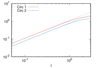
Figure 2: Nonlinear gravity perturbation characterized by $A_{tw}=1/3$ , $Re=10^{3}$ with (left) $B_{0}=2.5$ and (right) $B_{0}=-2.5$ : Circulations $\Gamma^{(1)}_{x\geq 0}(t)$, $\Gamma^{(2)}_{x\geq 0}(t)$ as a function of time. Numerical values from DNS simulations are displayed using solid lines, and theoretical values (84) by dashed lines.

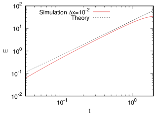
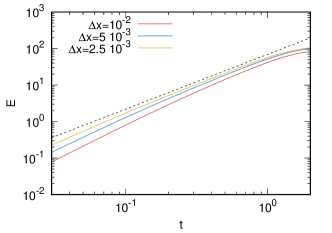
Figure 3: Nonlinear gravity perturbation characterized by $A_{tw}=1/3$ and $B_{0}=-2.5$ with (left) $Re=10^{3}$ and (right) $Re=10^{4}$: Temporal evolution of the total enstrophy $E$. solid lines are DNS simulations values and dashed lines ares theoretical values (84).

6.2 Qualitative explanation for time evolution

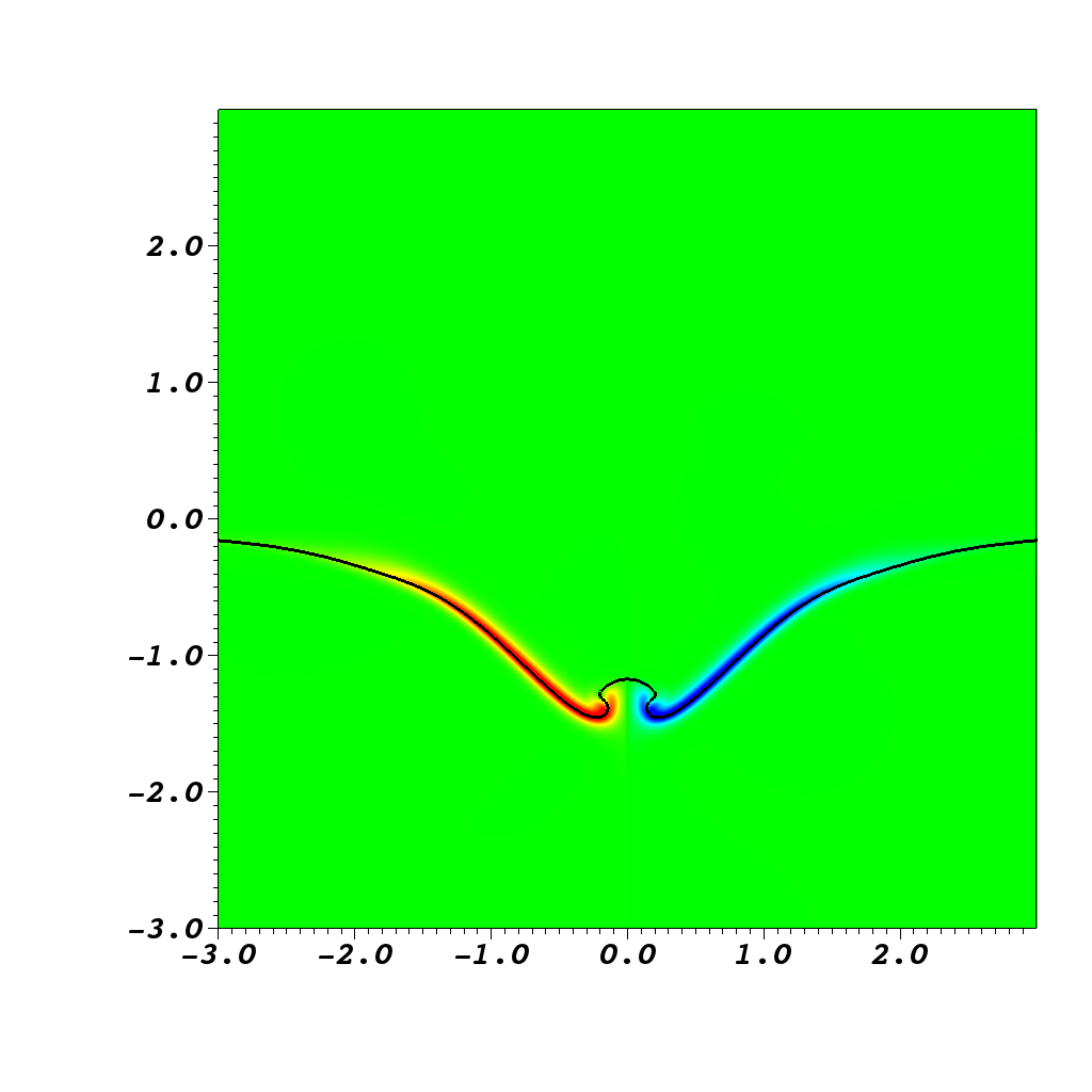
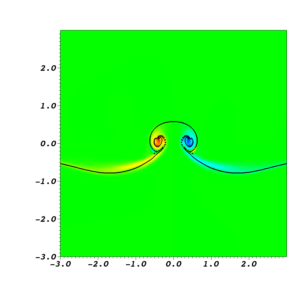
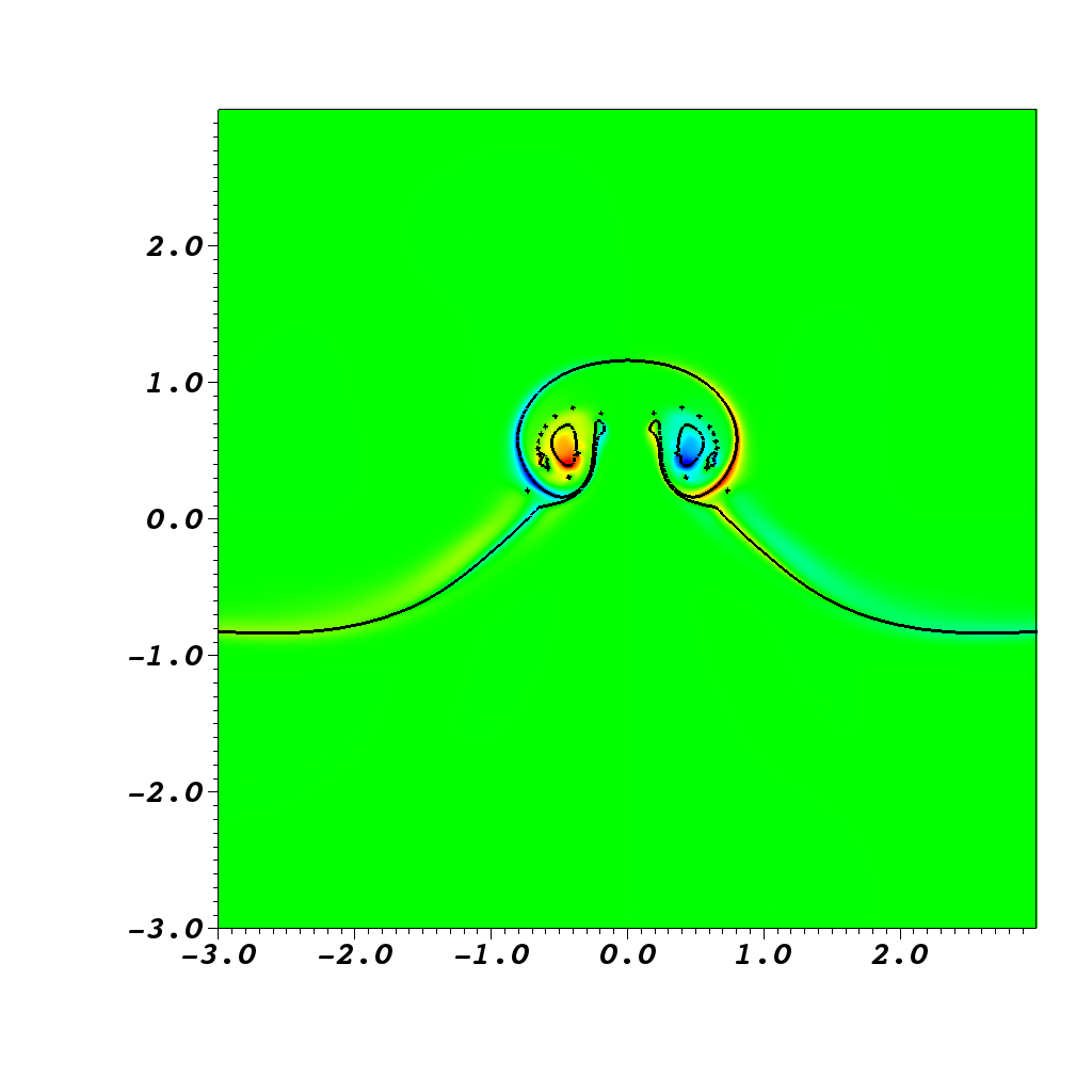
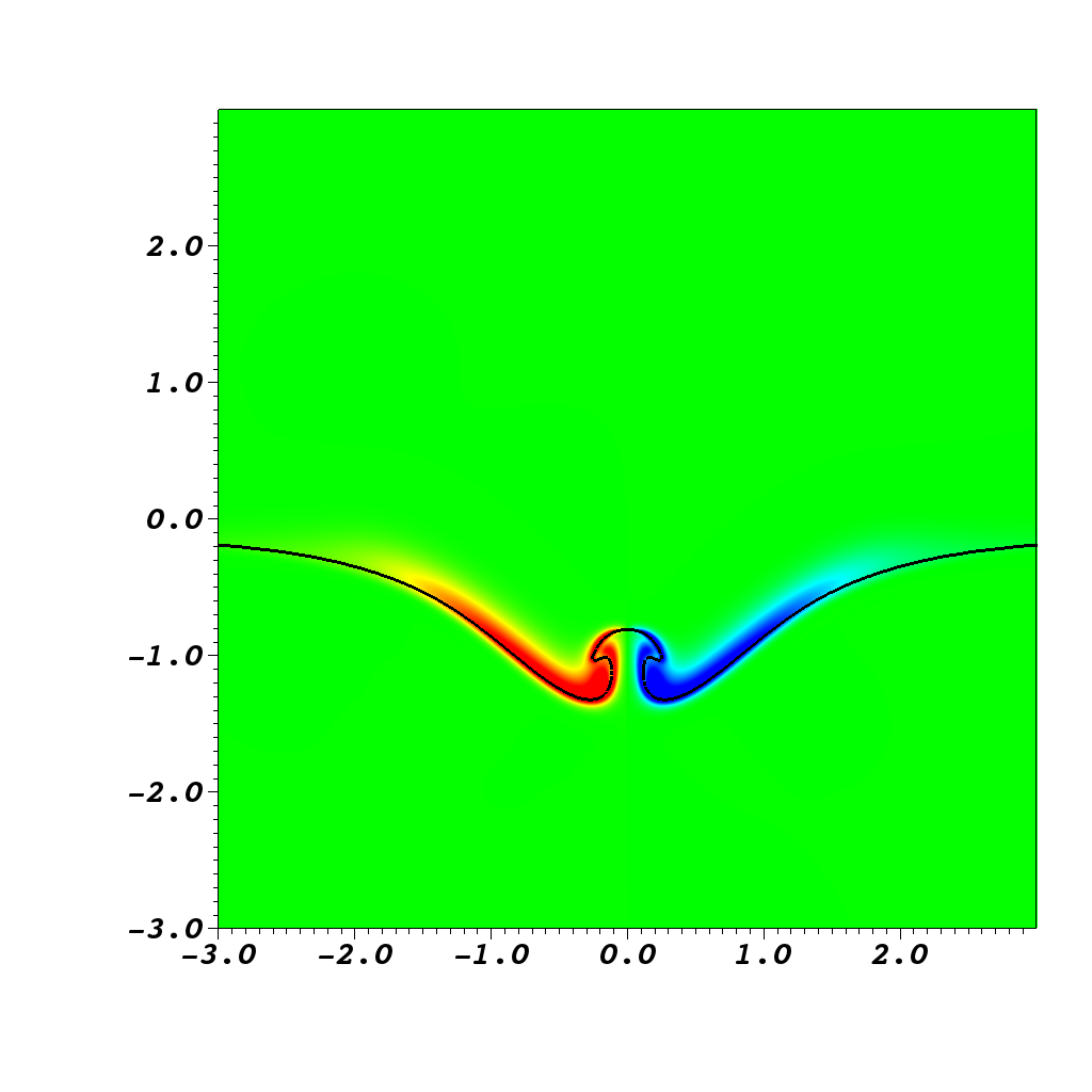
Figure 4: Nonlinear gravity perturbation characterized by $B_{0}=-2.5$, $Re=10^{3}$ with (top) $A_{tw}=1/3$ and (bottom) $A_{tw}=9/11$ : Snapshots of interface and vorticity field at dimensionless times $t=2,4,6$.

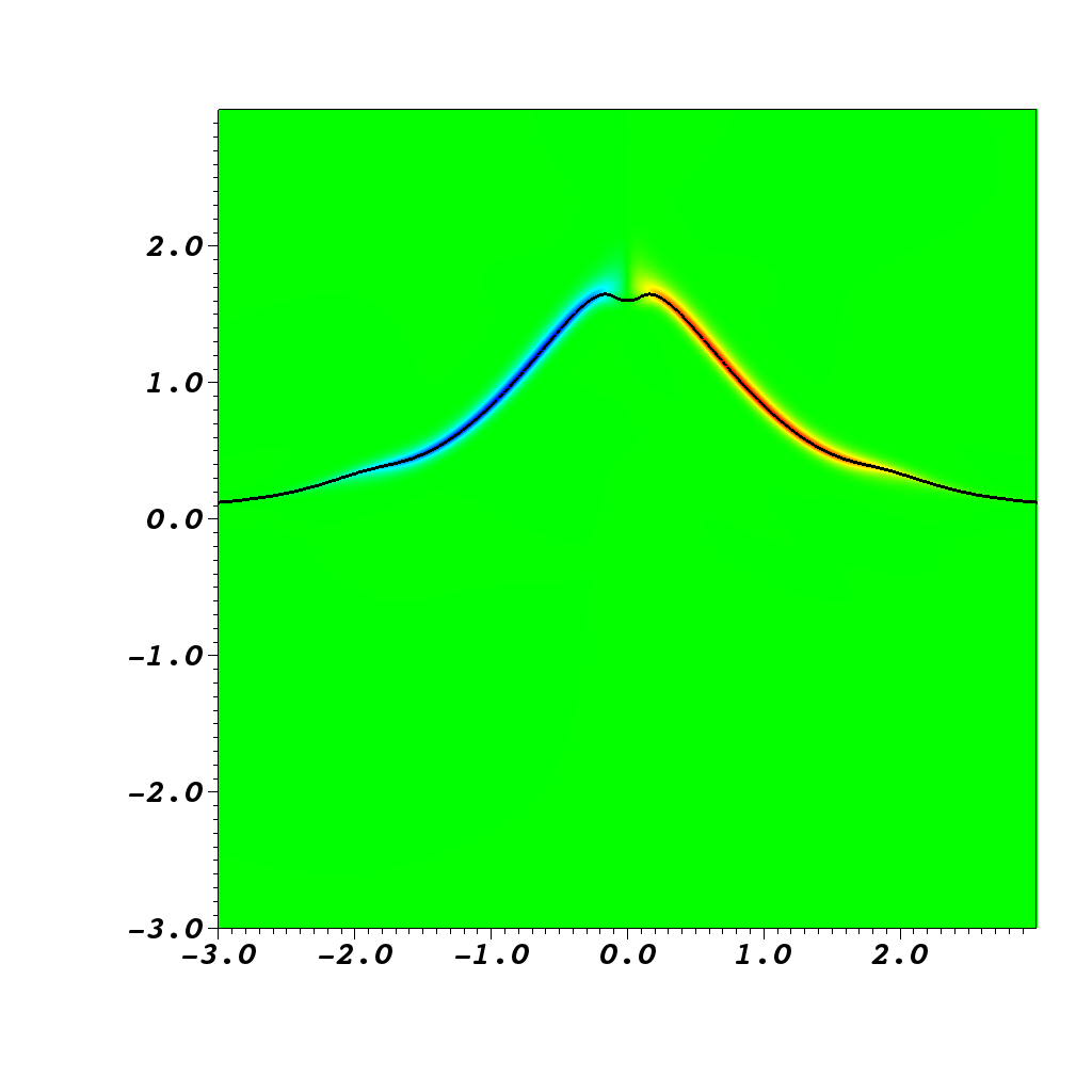
Figure 5: Idem than figure 4 but for $B_{0}=2.5$.

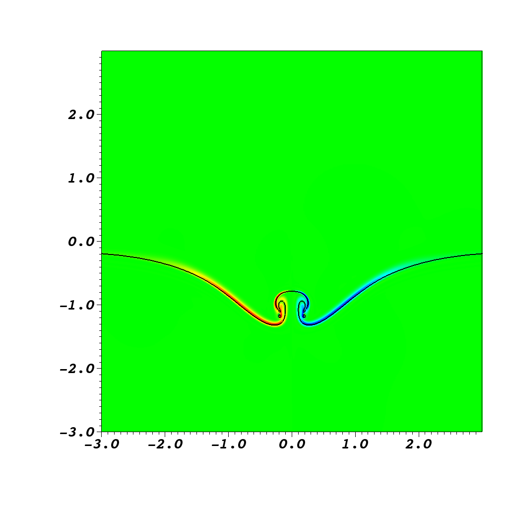
Figure 6: Nonlinear gravity perturbation characterized by $B_{0}=-2.5$, $Re=10^{4}$ and $A_{tw}=9/11$ : Snapshots of interface and vorticity field at dimensionless times $t=2,4,6$.

Figure 7: Idem than figure 6 but for $B_{0}=2.5$.

We focus now on the interface patterns. For $B_{0}<0$, the heavier fluid pushes the light phase forming a mushroom pattern (figure 4). The shape depends on the density ratio $r_{\rho}$ : the mushroom width decreases for increasing density ratio (figure 4). For $B_{0}>0$, the lighter fluid tends to penetrate the heavier one but the interface remains much flatter creating a crater-like structure (figure 5). This problem behaves differently with respect to the Reynolds dependency. For $B_{0}<0$, the Reynolds number (figure 6) is affecting the mushroom structure. For $B_{0}>0$, the dependency on the Reynolds number is not significant (figure 7). The interface evolution is induced by the vorticity generated on the interface itself which in turns depends on the source. However one may qualitatively justify the different behaviours observed by noting which source terms are dominant during each phase. When ${\rho^{(2)}}/\rho^{(1)}>>1$, we use equation (75) where we neglect the Reynolds part (we only consider problems where viscosity has a small influence on the total production rates, which is valid in the limit of infinite Reynolds) so that

$$\hat{\Psi}_{\Sigma}\approx{\hat{\Psi}}_{pot}+{\hat{\Psi}}_{\rho_{m}}~{}~{}~{}~{}\hbox{with}~{}~{}~{}\hat{\Psi}_{pot}=-\frac{\hat{\eta}}{\pi}.$$ (86)

Near $t=0$ the potential term ${\Psi}_{pot}$ is significant and the velocity term ${\Psi}_{\rho_{m}}$ is negligible. By contrast, when the interface amplitude becomes weaker and velocity is sufficiently large, ${\Psi}_{\rho_{m}}$ is dominant and ${\Psi}_{pot}$ negligible. Let us assume then a two step process. In a first period, the gravity source term ${\Psi}_{pot}$ only produces the vorticity field. In a second period, this vorticity field is modified by the total source. Using the approximate expression (156) and assuming it to be valid similar to the principal Fourier mode $k=\pi$ (this mode amplitude goes to zero at time $T_{f}=\pi/(2\hat{\varpi})$ for a pulsation $\hat{\varpi}=1$) then at $t=\frac{\pi}{2}$:

$$\omega(x,y,t)=\begin{cases}\omega^{(1)}(x,y)=-2\pi\frac{\Sigma^{(1)}_{A}(x)}{\sqrt{2}\delta^{(1)}}G(\frac{y}{\sqrt{2}\delta^{(1)}})~{}~{}&\text{if $y\geq 0$}\\ \omega^{(2)}(x,y)=-2\pi\frac{\Sigma^{(2)}_{A}(x)}{\sqrt{2}\delta^{(2)}}G(-\frac{y}{\sqrt{2}\delta^{(2)}})~{}~{}&\text{if $y\leq 0$}\end{cases}$$ (87)

with

$$G(z)\equiv-\frac{1}{\sqrt{\pi}}\exp(-z^{2})+z\bigg{[}1-Erf(z)\bigg{]}$$

and

$$\delta^{(1)}=\sqrt{1+r_{\rho}}\sqrt{\frac{\pi}{2Re}},~{}~{}~{}~{}~{}\delta^{(2)}=\sqrt{\frac{1+r_{\rho}}{r_{\rho}}}\sqrt{\frac{\pi}{2Re}}$$ (88)

$$\Sigma^{(1)}_{A}(x)=\frac{\sqrt{r_{\rho}}}{1+\sqrt{r_{\rho}}}\Sigma_{A}(x),~{}~{}\Sigma^{(2)}_{A}(x)=\frac{1}{1+\sqrt{r_{\rho}}}\Sigma_{A}(x)$$ (89)

$$\Sigma_{A}(x)=\frac{4B_{0}}{\pi}x\exp(-x^{2})$$ (90)

One then initializes a new simulation with two-dimensional vorticity field generated by this source.

Figure 8: Nonlinear gravity perturbation characterized by $A_{tw}=9/11$, $Re=10^{4}$ and (top) $B_{0}=2.5$, (bottom) $B_{0}=-2.5$: evolution of an initial flat interface at time $t=0,1,2$. An initial vorticity layer is present on the interface corresponding to equation (87).

The numerical simulations show that whether we reproduce the positive bump case or the negative bump case similar structures than those observed in the original problem are found(figure 8): in the case of $B_{0}<0$ a jet similar to that of figure 4 is observed, whereas for $B_{0}>0$ a crater like structure similar to that of figure 5 appears. To explain this non-symmetric behavior let us compute the source the numerical method of appendix A for a flat surface( to be called configuration B). In that instance, the two gravitational terms (with $\eta$ and $\Psi_{g}$) are zero and the inertial term dominates the vorticity flux.

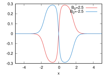
Figure 9: Nonlinear gravity perturbation characterized by $|B_{0}|=2.5$, $Re=\infty$ and $A_{tw}\to 1$: Sources $\Sigma$ in (left) configuration A (bump and flow at rest) and (right) configuration B (flat interface and velocity).

Figure 9 shows the structure of the sources in configuration A and B in the limiting case of $A_{tw}\to 1$. We first note that the term ${\Psi}_{pot}$ is symmetric with respect to the symmetry $\eta^{*}(x,t)=-\eta(x,t)$ and $(u^{*}_{1}(x,y,t),u^{*}_{2}(x,y,t))=(u_{1}(x,-y,t),-u_{2}(x,-y,t))$, while the term ${\Psi}_{\rho_{m}}$ is said to be antisymmetric, as the source has the same sign irrespective of the sign of the perturbation $B$. This has important consequences on the vorticity field and interface dynamics, as the non-linear term tends to modify the vorticity field differently upon the sign of $B$. Thus, while for $B<0$ non-linear terms tend to increase the intensity of vorticity production in the region $|x|<1$ and decreasing it in the outer region $|x|>1$, the opposite occurs for $B>0$. The direct consequence is that the two vorticity layers of opposite sign created at both sides of the x-axis preferentially roll-up near the axis creating a jet for $B<0$ while for $B>0$ the roll-up of the structure is induced in the outer region.

7 Conclusion.

In this work, we studied the production of vorticity at an interface separating two immiscible incompressible fluids for a two-dimensional flow. We proposed a new decomposition of the vorticity flux which makes explicit its dependence on parameters such as surface tension $\sigma$, viscosity $\mu$ and gravity $g$, the various factors are obtained by solving Laplace equations. In some cases, in particular the case $\rho^{(2)}/\rho^{(1)}<<1$ and $Re\gg 1$, it is possible to solve analytically most of these Laplace equations and to reduce the complexity of the procedure. This approach can a priori be extended to three-dimensional flows (we are currently working on this topic).

The case of gravito-capillary wave has been also discussed based on this procedure. Analytical as well as numerical examples have been presented. From the analytical side, it leads to results already known but from a new perspective. From the numerical perspective, it provides some quantitative predictions at short time that can be a good test for numerical codes or enables a qualitative understanding of numerical results.

Appendix A Numerical implementation for sources computations.

To evaluate the vorticity flux $\Sigma$, one should compute one Poisson equation and ten Laplace equations. The Poisson solver is easy to implement. For the five discontinuous fields $\Psi_{d\sigma}$, $\Psi_{dg}$, $\Psi_{d\rho}$, $\Psi_{d\mu}$, the boundary condition of Dirichlet type is imposed on a boundary with a known geometry. Practically, there exists immersed boundary methods that solve numerically such a problem ¹⁷; ²².

The remaining five fields $\Psi_{[[\rho]]}$, $\Psi_{\sigma}$, $\Psi_{g}$, $\Psi_{\mu_{m}}$, $\Psi_{[[\mu]]}$ are continuous across interface $(I)$ but the normal derivative of which is discontinuous across $(I)$ of the form $[[\upsilon n_{i}\partial_{i}\Phi]]=G$ (see conditions (36)–(38)). These five fields $\Psi_{\sigma}$, $\Psi_{g}$, $\Psi_{[[\rho]]}$ , $\Psi_{\mu_{m}}$, $\Psi_{[[\mu]]}$ can be obtained by numerical methods. In a volume of fluids approach, one solves the Laplace equation

$$\Delta\Psi=\nabla\cdot(\nabla\Psi)=0$$ (91)

in each domain away from the cell crossed by the interface boundary. For such cells containing an interface, special care is required so that the derivative discontinuity is used in integrating this equation. Each such cell is subdivided into two sub-cells $\Omega_{1}$ and $\Omega_{2}$ occupied for phase $1$ and $2$ respectively. Since in each subcell, Laplace equation is satisfied

$$\upsilon^{(1)}\int_{\Omega_{1}}\nabla\cdot(\nabla\Psi^{(1)})ds_{1}=0,~{}~{}~{}~{}~{}\upsilon^{(2)}\int_{\Omega_{2}}\nabla\cdot(\nabla\Psi^{(2)})ds_{2}=0$$ (92)

Now applying the divergence theorem in each phase and summing both expressions, yield

$$\upsilon^{(1)}\int_{S_{1}}\vec{n}^{(out)}\cdot\nabla\Psi^{(1)}dS_{1}+\upsilon^{(2)}\int_{S_{2}}\vec{n}^{(out)}\cdot\nabla\Psi^{(2)}dS_{2}+\int_{(I)}[[\vec{n}^{(1\to 2)}\cdot(\upsilon\nabla\Psi)]]dS=0.$$ (93)

where the closed surface of the cell is divided in $S_{1}$ in phase 1 and $S_{2}$ in phase 2 and $n^{(out)}$ is the outward unit normal vector. In addition let us called $(I)$ the portion of interface cutting the cell. For a quad/cube cell with face surface $\Delta S_{f}$ crossed by an interface of length $\Delta S_{I}$ we readily obtain

$$\sum_{f}\vec{n}^{(out)}\cdot\bigg{(}\upsilon^{(1)}\nabla\Psi^{(1)}\bigg{)}c_{f}+\sum_{f}\vec{n}^{(out)}\cdot\bigg{(}\upsilon^{(2)}\nabla\Psi^{(2)}\bigg{)}(1-c_{f})=-G\frac{\Delta S_{I}}{\Delta S_{f}}$$ (94)

where $n^{1\to 2}$ is the unit normal to the interface pointing from fluid 1 to fluid 2, $c_{f}$ is the face fraction of the fluid 1 crossing a given face and

$$G\equiv[[\upsilon\vec{n}^{(1\to 2)}\cdot\nabla\Psi]],$$ (95)

is given by (36)–(37)–(38). This numerical approach is used in the computation of the different sources in section 6 which assumes also continuity of function $\Psi$ crossing the interface. It is equivalent to solve the variable coefficient Poisson equation

$$\nabla\cdot(\upsilon\nabla\Psi)=-G\delta({n}^{(1\to 2)})$$ (96)

Appendix B Asymptotic case $A_{tw}\to 1$.

In this appendix, we work in dimensionless variables and study functions $\Psi_{x}$ ($x=\sigma,g,\rho,\rho_{m},\mu_{m},[[\mu]]$) when fluid 1 is much lighter than fluid 2 i.e. ${\rho^{(2)}}>>\rho^{(1)}$ and $\nu^{(2)}/\nu^{(1)}$ is of order one. A small parameter $\epsilon\equiv\frac{\upsilon^{(2)}}{\upsilon^{(1)}}=\frac{\rho^{(1)}}{\rho^{(2)}}<<1$ exists. Note the relations $\epsilon=\frac{1-A_{tw}}{1+A_{tw}}$ and

$$\frac{[[\upsilon]]\mu_{m}}{\nu_{m}}=-\epsilon\frac{\nu^{(1)}}{\nu^{(1)}+\nu^{(2)}}+\frac{\nu^{(1)}-\nu^{(2)}}{\nu^{(1)}+\nu^{(2)}}+\frac{1}{\epsilon}\frac{\nu^{(2)}}{\nu^{(1)}+\nu^{(2)}}$$ (97)

$$\frac{[[\upsilon]]~{}[[\mu]]}{\nu_{m}}=-\epsilon\frac{2\nu^{(1)}}{\nu^{(1)}+\nu^{(2)}}+2-\frac{1}{\epsilon}\frac{2\nu^{(2)}}{\nu^{(1)}+\nu^{(2)}}$$ (98)

$$\frac{\upsilon_{m}[[\mu]]}{\nu_{m}}=\epsilon\frac{\nu^{(1)}}{\nu^{(1)}+\nu^{(2)}}+\frac{\nu^{(1)}-\nu^{(2)}}{\nu^{(1)}+\nu^{(2)}}-\frac{1}{\epsilon}\frac{\nu^{(2)}}{\nu^{(1)}+\nu^{(2)}}.$$ (99)

When $A_{tw}\to 1$, $\epsilon\approx\frac{1-A_{tw}}{2}$

First functions $\Psi_{d\sigma}$, $\Psi_{dg}$, $\Psi_{d\rho}$ do not depend on the density ratio $\epsilon$ and all vary over a characteristic length scale $L_{0}$. Second the boundary condition for $\Psi_{x}$ with $x=\sigma,g,\rho$ reads

$$n_{i}\partial_{i}(\Psi^{(1)}_{x}+\Psi^{(1)}_{dx})=\epsilon n_{i}\partial_{i}(\Psi^{(2)}_{x}+\Psi^{(2)}_{dx})$$ (100)

Since $\Psi^{(1)}_{dx}$ and $\Psi^{(2)}_{dx}$ are both harmonic and $\Psi^{(1)}_{dx}=-\Psi^{(2)}_{dx}$ along the interface, these functions must vary with the same characteristic length $L_{0}$. This leads to the simplification

$$n_{i}\partial_{i}(\Psi^{(1)}_{x}+\Psi^{(1)}_{dx})=\epsilon n_{i}\partial_{i}(\Psi^{(2)}_{x})$$ (101)

Similarly $\Psi^{(1)}_{x}$ and $\Psi^{(2)}_{x}$ are harmonic and $\Psi^{(1)}_{x}=\Psi^{(2)}_{x}$ on the interface: these functions vary with the same characteristic length hence a further simplification

$$n_{i}\partial_{i}(\Psi^{(1)}_{x}+\Psi^{(1)}_{dx})=0,~{}~{}~{}\hbox{for }~{}~{}~{}x=\sigma,g,\rho$$ (102)

Fields $\Psi_{\sigma}$, $\Psi_{g}$, $\Psi_{[[\rho]]}$ hence verify continuity across the interface and the above simplified conditions. It is easily seen that this leads to

$$\Psi_{x}^{(1)}=-\Psi^{(1)}_{dx},~{}~{}~{}~{}\Psi_{x}^{(2)}=\Psi^{(2)}_{dx}~{}~{}~{}\hbox{for }~{}~{}~{}x=\sigma,g,\rho$$ (103)

Because of conditions (35), this imposes at the interface

$$\Psi_{\sigma}=\frac{\kappa}{2},~{}~{}~{}\Psi_{g}=-\frac{\eta}{2},~{}~{}~{}~{}\Psi_{[[\rho]]}=\frac{1}{2}{\Psi_{\rho_{m}}},$$ (104)

It is thus not necessary to solve Laplace equations for $\Psi_{\sigma}$, $\Psi_{g}$, or $\Psi_{[[\rho]]}$ in such an approximation. On the interface, this yields

$$\hat{\Psi}_{\Sigma}=-\frac{1}{2}\frac{\kappa}{We}-Fr~{}\hat{\eta}+\hat{\Psi}_{\rho_{m}}+\Psi_{\rm{visc}}$$ (105)

where the term $\Psi_{\rm{visc}}$ is related to viscous effects discussed below.

In addition, $\Psi_{\mu_{m}}$ satisfies Laplace equation and

$$n_{i}\partial_{i}(\Psi^{(1)}_{\mu_{m}})-\epsilon n_{i}\partial_{i}(\Psi^{(2)}_{\mu_{m}})=n_{i}\partial_{j}\partial_{j}u^{(1)}_{i}-\epsilon n_{i}\partial_{j}\partial_{j}u^{(2)}_{i}$$ (106)

Since $\Psi_{\mu_{m}}$ is a harmonic function and continuous across the surface then one may neglect the second l.h.s. term

$$n_{i}\partial_{i}(\Psi^{(1)}_{\mu_{m}})=n_{i}\partial_{j}\partial_{j}u^{(1)}_{i}-\epsilon n_{i}\partial_{j}\partial_{j}u^{(2)}_{i}$$ (107)

Condition $Re>>1$

When $Re>>1$ and $\nu^{(2)}/\nu^{(1)}=O(1)$, a boundary layer is present of dimensionless size $\delta^{(r)}=\frac{\nu^{(r)}}{\nu_{m}}\sqrt{Re}$ in each phase and of comparable width. It is however a weak boundary layer since vorticity is of order one contrary to the boundary layer on a solid. Hence quantity $n_{i}\partial_{j}\partial_{j}u^{(r)}_{i}$ could be of order $O(\sqrt{Re})$ or less for both phases and the second term of the r.h.s. of equation (107) may be again neglected compared to the first of the r.h.s.

$$n_{i}\partial_{i}(\Psi^{(1)}_{\mu_{m}})=n_{i}\partial_{j}\partial_{j}u^{(1)}_{i}$$ (108)

In that approximation, one only solves the Laplace equation in the phase 1 with the above Neumann condition. Furthermore we need $\Psi^{(2)}_{\mu_{m}}$ on the interface. This value is given by the Dirichlet condition $\Psi^{(2)}_{\mu_{m}}=\Psi^{(1)}_{\mu_{m}}$. The field $\Psi_{d\mu}$ satisfies Laplace equation and

$$\Psi^{(1)}_{d\mu}=-\Psi^{(2)}_{d\mu}=\bigg{(}\kappa\vec{u}\cdot\vec{n}-\,\vec{t}\cdot\vec{\nabla}(\vec{u}\cdot\vec{t})\bigg{)}$$ (109)

It is of order $O(1)$. Finally function $\Psi_{[[\mu]]}+\Psi_{d\mu}$ is harmonic, and satisfies along the interface

$$n_{i}\partial_{i}(\Psi^{(1)}_{[[\mu]]}+\Psi^{(1)}_{d\mu})-\epsilon n_{i}\partial_{i}(\Psi^{(2)}_{[[\mu]]}+\Psi^{(2)}_{d\mu})=\frac{1}{2}\bigg{(}n_{i}\partial_{j}\partial_{j}u^{(1)}_{i}+\epsilon n_{i}\partial_{j}\partial_{j}u^{(2)}_{i}\bigg{)}$$ (110)

One neglects the second r.h.s term as above if $\nu^{(2)}/\nu^{(1)}=O(1)$. In addition, because of its continuity, $\Psi_{[[\mu]]}$ varies along the interface in a similar manner in both domain so that one may neglect the second l.h.s. term

$$n_{i}\partial_{i}\Psi^{(1)}_{[[\mu]]}=-n_{i}\partial_{i}\big{(}\Psi^{(1)}_{d\mu}-\frac{1}{2}\Psi^{(1)}_{\mu_{m}}]\big{)}$$ (111)

This is solved in domain fluid 1

$$\Psi^{(1)}_{[[\mu]]}=-\Psi^{(1)}_{d\mu}+\frac{1}{2}\Psi^{(1)}_{\mu_{m}}.$$ (112)

The continuity of $\Psi_{[[\mu]]}$ across the interface then implies

$$\Psi^{(2)}_{[[\mu]]}=\Psi^{(2)}_{d\mu}+\frac{1}{2}\Psi^{(2)}_{\mu_{m}}.$$ (113)

For $Re>>1$, $\hat{\Psi}_{\mu_{m}}$, $\hat{\Psi}_{[[\mu]]}$ are of order $O(\sqrt{Re})$. Using expansions (97), (98), (99) and relation (112), the term $\Psi_{\rm{visc}}$ in equation (4) is of order $O(1/\sqrt{Re}$) and

$$\Psi_{\Sigma}\approx-\frac{1}{2}\frac{\kappa}{We}-Fr~{}\hat{\eta}+\hat{\Psi}_{\rho_{m}}~{}~{}~{}\hbox{for}~{}~{}~{}Re>>1$$ (114)

Stokes condition $Re<<1$

When $Re<<1$ and $\nu^{(2)}/\nu^{(1)}=O(1)$, the quantity $n_{i}\partial_{j}\partial_{j}u^{(r)}_{i}$ is of the same order for both phases and the second term in the r.h.s. may be hence again neglected.

$$n_{i}\partial_{i}(\Psi^{(1)}_{\mu_{m}})=n_{i}\partial_{j}\partial_{j}u^{(1)}_{i}$$ (115)

In that approximation, one only solves the Laplace equation in the phase 1, with the Neumann condition

$$n_{i}\partial_{i}\Psi^{(1)}_{\mu_{m}}=n_{i}\partial_{j}\partial_{j}u^{(1)}_{i}$$ (116)

which depends on phase 1 only. Furthermore we need $\Psi^{(2)}_{\mu_{m}}$ on the interface. This value is given by the Dirichlet condition $\Psi^{(2)}_{\mu_{m}}=\Psi^{(1)}_{\mu_{m}}$. The field $\Psi_{d\mu}$ satisfies Laplace equation and

$$\Psi^{(1)}_{d\mu}=-\Psi^{(2)}_{d\mu}=\bigg{(}\kappa\vec{u}\cdot\vec{n}-\,\vec{t}\cdot\vec{\nabla}(\vec{u}\cdot\vec{t})\bigg{)}$$ (117)

Finally function $\Psi_{[[\mu]]}+\Psi_{d\mu}$ is harmonic, and satisfies along the interface

$$n_{i}\partial_{i}(\Psi^{(1)}_{[[\mu]]}+\Psi^{(1)}_{d\mu})-\epsilon n_{i}\partial_{i}(\Psi^{(2)}_{[[\mu]]}+\Psi^{(2)}_{d\mu})=\frac{1}{2}\bigg{(}n_{i}\partial_{j}\partial_{j}u^{(1)}_{i}+\epsilon n_{i}\partial_{j}\partial_{j}u^{(2)}_{i}\bigg{)}$$ (118)

One neglects the second r.h.s term as above if $\nu^{(2)}/\nu^{(1)}=O(1)$. In addition, because of its continuity, $\Psi_{[[\mu]]}$ varies along the interface in a similar manner in both domain so that one may neglect the second l.h.s. term

$$n_{i}\partial_{i}\Psi^{(1)}_{[[\mu]]}=-n_{i}\partial_{i}\big{(}\Psi^{(1)}_{d\mu}-\frac{1}{2}\Psi^{(1)}_{\mu_{m}}]\big{)}$$ (119)

This is solved in domain fluid 1

$$\Psi^{(1)}_{[[\mu]]}=-\Psi^{(1)}_{d\mu}+\frac{1}{2}\Psi^{(1)}_{\mu_{m}}.$$ (120)

The continuity of $\Psi_{[[\mu]]}$ across the interface then implies

$$\Psi^{(2)}_{[[\mu]]}=\Psi^{(2)}_{d\mu}+\frac{1}{2}\Psi^{(2)}_{\mu_{m}}.$$ (121)

As a consequence on the interface at order zero

$$\Psi_{[[\mu]]}=-\bigg{(}\kappa\vec{u}\cdot\vec{n}-\,\vec{t}\cdot\vec{\nabla}(\vec{u}\cdot\vec{t})\bigg{)}+\frac{1}{2}\Psi_{\mu_{m}}.$$ (122)

Replacing these expressions into the full vorticity source we readily find that the source is zero at leading order and therefore it is required to obtain the functions at the next order, requiring to evaluate them numerically in a general case. As a conclusion, although for $Re<<1$ the viscous terms are always preponderant and control the vorticity production

$$\hat{\Psi}_{\Sigma}\approx\Psi_{2}.$$

Note that there is no obvious advantage between computing the first order approximation and the full expression for Eq. 4.

Appendix C Source field for viscous capillary gravity waves.

We start by expressing coefficients $A^{(1)}$, $B^{(1)}$, $A^{(2)}$, $B^{(2)}$ as a function of $\eta_{0}$. Note that the tangential velocity field is continuous across the interface. After linearization this implies

$$ikA^{(1)}+\kappa^{(1)}B^{(1)}=ikA^{(2)}-\kappa^{(2)}B^{(2)}$$ (123)

The linearized kinematic condition at the interface

$$\partial_{t}\eta=\partial_{y}\phi^{(r)}(x,y=0,t)+\partial_{x}\psi^{(r)}(x,y=0,t),~{}~{}~{}~{}r=1,2;$$ (124)

yields two supplementary relations

$$B^{(1)}=-\frac{\varpi}{k}\eta_{0}-i\frac{|k|}{k}A^{(1)};~{}~{}~{}~{}~{}B^{(2)}=-\frac{\varpi}{k}\eta_{0}+i\frac{|k|}{k}A^{(2)}$$ (125)

Finally the jump on vorticity in its linearized form

$$[[\mu{\omega}_{z}]]=-[[2\mu]]\frac{\partial u_{y}}{\partial x}=-ik[[2\mu]]u_{y}$$ (126)

yields the fourth equation

$$\mu^{(1)}\big{(}2ik|k|A^{(1)}+[k^{2}+(\kappa^{(1)})^{2}]B^{(1)}\big{)}=\mu^{(2)}\big{(}-2ik|k|A^{(2)}+[k^{2}+(\kappa^{(2)})^{2}]B^{(2)}\big{)}$$ (127)

The solution of the system yields

$$|k|A^{(1)}=i\varpi\eta_{0}-2k\frac{i\varpi\rho^{(2)}+k[[\mu]]b^{(2)}}{\rho^{(2)}b^{(1)}+\rho^{(1)}b^{(2)}}\eta_{0},$$ (128)

$$|k|A^{(2)}=-i\varpi\eta_{0}+2k\frac{i\varpi\rho^{(1)}-k[[\mu]]b^{(1)}}{\rho^{(2)}b^{(1)}+\rho^{(1)}b^{(2)}}\eta_{0},$$ (129)

Let us now compute $\Sigma$ using the source terms in (55) i.e. $\Psi_{\sigma}$, $\Psi_{g}$, $\Psi_{\mu_{m}}$, $\Psi_{[[\mu]]}$ and ${u}_{x}$. It is easy to understand that a field $\Psi_{q}$ where $q$ is selected among one of sources ${d\sigma}$, ${dg}$, ${d\mu}$, ${\sigma}$, ${g}$, ${\mu_{m}}$ or ${[[\mu]]}$, satisfies a Laplace equation within the two fluid phases. As the consequence, this imposes

$$\Psi_{q}=\begin{cases}A^{(1)}_{q}\exp{\bigg{(}i(kx-\varpi(k)t)-\mid k\mid y\bigg{)}}&\text{if $0<y$}\\ A^{(2)}_{q}\exp{\bigg{(}i(kx-\varpi(k)t)+\mid k\mid y\bigg{)}}&\text{if $y\leq 0$}\end{cases}$$ (130)

Replacing these values in equation (55) yields $\Sigma=ik\Psi_{\Sigma}\exp{i(kx-\varpi(k)t)}$ with

$${\Psi_{\Sigma}}_{0}=\bigg{(}-\sigma\upsilon_{m}k^{2}\eta_{0}+[[\upsilon]]\big{(}\sigma A_{\sigma}+g[[\rho]]A_{g}-\rho_{m}g\eta_{0}\big{)}\bigg{)}+[[\upsilon]]\mu_{m}A_{\mu_{m}}+[[\mu]]\bigg{(}-\,2\upsilon_{m}\,iku_{x}+[[\upsilon]]A_{[[\mu]]}\bigg{)}$$ (131)

For infinitesimal amplitudes, the boundary conditions for the various $\Psi_{q}$ fields should be linearized at $y=0$. By matching these conditions, the constants of fields $\Psi_{dg}$, $\Psi_{g}$, $\Psi_{d\sigma}$ and $\Psi_{\sigma}$ in the Laplace equations (130) are found.

The boundary conditions for fields $\Psi_{dg}$ and $\Psi_{d\sigma}$ linearized at $y=0$ read

$$\Psi^{(1)}_{dg}(y=0,t)=-\Psi^{(2)}_{dg}(y=0,t)=\frac{\eta_{0}}{2},~{}~{}~{}~{}\Psi^{(1)}_{d\sigma}(y=0,t)=-\Psi^{(2)}_{d\sigma}(y=0,t)=-k^{2}\frac{\eta_{0}}{2}.$$ (132)

This implies that $\Psi_{d\sigma}=-k^{2}\Psi_{dg}$. The Laplace equation with the above conditions leads to

$$A^{(1)}_{dg}=\frac{\eta_{0}}{2},~{}~{}~{}~{}~{}~{}A^{(2)}_{dg}=-\frac{\eta_{0}}{2}$$ (133)

Thereafter one introduces these expressions in the linearized boundary conditions of $\Psi_{g}$ yielding

$$A_{g}=-A_{tw}\frac{\eta_{0}}{2},~{}~{}~{}~{}\Psi_{\sigma}=-k^{2}\Psi_{g}.$$ (134)

The source can be thus simplified

$${\Psi_{\Sigma}}_{0}=-2\frac{\varpi^{2}_{inv}(k)}{|k|}\eta_{0}+[[\upsilon]]\mu_{m}A_{\mu_{m}}+[[\mu]]\bigg{(}-2\upsilon_{m}\,iku_{x}+[[\upsilon]]A_{[[\mu]]}\bigg{)}$$ (135)

The field $\Psi_{\mu_{m}}$ satisfies the linearized version of continuity and condition (37)

$$\Psi^{(1)}_{\mu_{m}}(y=0)=\Psi^{(2)}_{\mu_{m}}(y=0)~{}~{}~{}\hbox{and}~{}~{}~{}[[\upsilon\frac{\partial}{\partial y}\Psi_{\mu_{m}}]]=[[\partial_{j}\partial_{j}(\upsilon u_{y})]]$$ (136)

The two conditions reads

$$A_{\mu_{m}}=\frac{\varpi^{2}}{2|k|\upsilon_{m}}\bigg{(}\frac{1}{\mu^{(1)}}-\frac{1}{\mu^{(2)}}\bigg{)}\eta_{0}+i\frac{\varpi}{2\upsilon_{m}}\bigg{(}\frac{1}{\mu^{(1)}}A^{(1)}+\frac{1}{\mu^{(2)}}A^{(2)}\bigg{)}$$ (137)

The field $\Psi_{d\mu}$ satisfies the Dirichlet condition (35) which once linearized, imposes

$$\Psi^{(1)}_{d\mu}(y=0)=-\Psi^{(2)}_{d\mu}(y=0)=-\,ik{u}_{x}(y=0)$$ (138)

The continuity (123) of velocity component $u_{x}$ across the interface imposes

$$A^{(1)}_{d\mu}=(k^{2}-\kappa^{(1)}|k|)A^{(1)}+i\kappa^{(1)}\varpi\eta_{0}$$ (139)

$$A^{(2)}_{d\mu}=-(k^{2}-\kappa^{(2)}|k|)A^{(2)}+i\kappa^{(2)}\varpi\eta_{0}$$ (140)

The field $\Psi_{[[\mu]]}$ satisfies continuity and condition (38) linearized across the interface. The first condition leads to $\Psi^{(1)}(y=0)=\Psi^{(2)}(y=0)$ that is $A^{(1)}_{[[\mu]]}=A^{(2)}_{[[\mu]]}$. The second condition at $y=0$ yields

$$[[\upsilon\frac{\partial}{\partial y}\Psi_{[[\mu]]}]]=-[[\upsilon\frac{\partial}{\partial y}\Psi_{d\mu}]]+\frac{1}{2}\bigg{(}\partial_{j}\partial_{j}(\upsilon^{(1)}u^{(1)}_{y})+\partial_{j}\partial_{j}(\upsilon^{(2)}u^{(2)}_{y})\bigg{)}$$ (141)

which can be rewritten as

$$A_{[[\mu]]}=-A_{tw}A^{(1)}_{d\mu}+A^{\prime}_{[[\mu]]},$$ (142)

$$A^{\prime}_{[[\mu]]}=\frac{1}{2|k|}\bigg{(}\frac{1}{\mu^{(1)}}+\frac{1}{\mu^{(2)}}\bigg{)}\frac{\varpi^{2}}{2\upsilon_{m}}\eta_{0}+i\frac{\varpi}{4\upsilon_{m}}\bigg{(}\frac{1}{\mu^{(1)}}A^{(1)}-\frac{1}{\mu^{(2)}}A^{(2)}\bigg{)}.$$ (143)

By summing these various sources, the total source becomes after some algebraic manipulations

$$\Psi_{\Sigma}=\alpha_{0}\eta_{0}+\alpha_{1}A^{(1)}+\alpha_{2}A^{(2)}$$ (144)

$$\alpha_{0}=-2\frac{\varpi^{2}_{inv}}{|k|}+\frac{[[\mu]]}{\rho_{m}}i(\kappa^{(1)}-\kappa^{(2)})\varpi$$ (145)

$$\alpha_{1}=iA_{tw}\varpi+\frac{[[\mu]]}{\rho_{m}}(k^{2}-\kappa^{(1)}|k|)$$ (146)

$$\alpha_{2}=iA_{tw}\varpi+\frac{[[\mu]]}{\rho_{m}}(k^{2}-\kappa^{(2)}|k|)$$ (147)

where the values of coefficients $A^{(1)}$ and $A^{(2)}$ are given in Eqs. 128-129.

Appendix D Computations near time $t=0$ for viscous gravity waves.

Here we work in dimensionless units. It is recalled that the curvilinear variable $s$ increases along $\vec{t}^{1\to 2}$ and the orthogonal variable $s_{\perp}$ increases along $\vec{n}^{1\to 2}$ in the Frenet-Serret frame. Let us evaluate the circulation per unit length produced during the time period near time $t=0$ in each monophasic domain

$$\gamma^{(1)}=\int^{0}_{-\infty}\omega^{(1)}\,\text{d}s_{\perp}~{}~{}~{}~{}~{}\gamma^{(2)}=\int^{\infty}_{0}\omega^{(2)}\,\text{d}s_{\perp}$$ (148)

In that period, the fluid is almost at rest and vorticity is zero initially. As a consequence equations (7) read

$$\frac{\partial}{\partial t}\left(\int_{A^{(r)}}\omega\,\text{d}x\text{d}y\right)=-\int_{(C_{r})}J^{(r)}_{j}\,n_{j}\,\text{d}s_{c}+\int_{(I)}\Sigma^{(r)}\,\text{d}s,~{}~{}~{}r=1,2$$ (149)

where the loop is the union of $(I)$ a stretch $ds$ along the interface and $(C_{r})$ made of two lines along the $s_{\perp}$-axis in fluid $r$ closing at infinity.

D.1 Computations near time $t=0$ discarding diffusion along the interface.

The r.h.s term becomes non zero and provides in each phase

$$\frac{\partial\gamma^{(1)}}{\partial t}=\frac{1+r_{\rho}}{2}\frac{1}{Re}\frac{\partial^{2}\gamma^{(1)}}{\partial s^{2}}+{\Sigma}^{(1)}(s,0),$$ (150)

$$\frac{\partial\gamma^{(2)}}{\partial t}=\frac{1+r_{\rho}}{2r_{\rho}}\frac{1}{Re}\frac{\partial^{2}\gamma^{(2)}}{\partial s^{2}}+{\Sigma}^{(2)}(s,0).$$ (151)

When discarding diffusion along the interface, one obtains near time $t=0$

$$\gamma^{(r)}(s,t)={\Sigma}^{(r)}(s,0)~{}t,~{}~{}~{}~{}r=1,2$$ (152)

This implies that the circulation in phase $r$ in the half plane $x\geq 0$ evolves according to

$$\Gamma^{(r)}_{x\geq 0}(t)=\bigg{(}\int_{(I),~{}x\geq 0}{\Sigma}^{(r)}(s,0)\,ds\bigg{)}~{}t,~{}~{}~{}~{}r=1,2$$ (153)

To go a step further, we may evaluate the vorticity produced during the first instants. Since the velocity field is almost zero, equation (3) implies that vorticity obeys a pure diffusion equation in the normal direction to the interface at any point of the interface with a Neumann boundary condition at the interface which is nothing but equation (12) : for $s_{\perp}\leq 0$

$$\partial_{t}\omega^{(1)}(s,t)=\frac{1+r_{\rho}}{2}\frac{1}{Re}\partial^{2}_{s_{\perp}}\omega^{(1)},~{}~{}~{}~{}\frac{1+r_{\rho}}{2}\frac{1}{Re}\partial_{s_{\perp}}\omega=\Sigma^{(1)}_{A}(s,t=0)$$ (154)

for $s_{\perp}\geq 0$

$$\partial_{t}\omega^{(2)}(s,t)=\frac{1+r_{\rho}}{2r_{\rho}}\frac{1}{Re}\partial^{2}_{s_{\perp}}\omega^{(2)},~{}~{}~{}~{}~{}~{}-\frac{1+r_{\rho}}{2r_{\rho}}\frac{1}{Re}\partial_{s_{\perp}}\omega=\Sigma^{(2)}_{A}(s,t=0)$$ (155)

The solution of these two equations are known to be

$$\omega(s,s_{\perp},t)=\begin{cases}\omega^{(1)}(s,s_{\perp},t)=-4\frac{\Sigma^{(1)}_{A}(s,t=0)}{\sqrt{2}\delta^{(1)}}G(-\frac{s_{\perp}}{\sqrt{2}\delta^{(1)}})~{}t~{}~{}&\text{if $s_{\perp}\leq 0$}\\ \omega^{(2)}(s,s_{\perp},t)=-4\frac{\Sigma^{(2)}_{A}(s,t=0)}{\sqrt{2}\delta^{(2)}}G(\frac{s_{\perp}}{\sqrt{2}\delta^{(2)}})~{}t~{}~{}&\text{if $s_{\perp}\geq 0$}\end{cases}$$ (156)

with

$$G(x)\equiv\int^{x}_{0}\bigg{[}1-Erf(x)\bigg{]}dx^{\prime}-\frac{1}{\sqrt{\pi}}=-\frac{1}{\sqrt{\pi}}\exp(-x^{2})+x\bigg{[}1-Erf(x)\bigg{]}$$

and

$$\delta^{(1)}=\sqrt{1+r_{\rho}}\sqrt{\frac{t}{Re}},~{}~{}~{}~{}~{}\delta^{(2)}=\sqrt{\frac{1+r_{\rho}}{r_{\rho}}}\sqrt{\frac{t}{Re}}$$ (157)

Since there is no jump of vorticity at interface because $[[\mu]]=0$ and since

$$\hbox{when}~{}~{}~{}~{}x~{}\to~{}~{}0,~{}~{}~{}G(x)~{}\to~{}-\frac{1}{\sqrt{\pi}},~{}~{}~{}~{}~{}~{}~{}~{}\int^{\infty}_{0}G(z)dz=-\frac{1}{4}$$

It is easily found that

$$\Sigma^{(1)}(s,t=0)=\sqrt{r_{\rho}}\Sigma^{(2)}(s,t=0)$$

Since $\Sigma=\Sigma^{(1)}+\Sigma^{(2)}$

$$\Sigma^{(1)}(s,t=0)=\frac{\sqrt{r_{\rho}}}{1+\sqrt{r_{\rho}}}\Sigma(s,t=0),~{}~{}\Sigma^{(2)}(s,t=0)=\frac{1}{1+\sqrt{r_{\rho}}}\Sigma(s,t=0)$$ (158)

Using these expressions, the circulation in each phase for $x\geq 0$ evolves according to

$$\Gamma^{(1)}_{x\geq 0}=\sqrt{r_{\rho}}\Gamma^{(2)}_{x\geq 0},~{}~{}~{}~{}~{}\Gamma^{(2)}_{x\geq 0}=\frac{1}{(1+\sqrt{r_{\rho}})}\bigg{(}\int_{(I),~{}x\geq 0}{\Sigma}(s,0)\,ds\bigg{)}~{}t,$$ (159)

and enstrophy $E$ in the whole domain according to

$$E=\int\int\omega^{2}dxdy=\int\int\omega^{2}dsds_{\perp}=I(r_{\rho})\bigg{(}\int(\Sigma)^{2}ds\bigg{)}~{}\sqrt{Re}~{}t^{3/2}$$ (160)

with

$$I(r_{\rho})=\frac{16}{\sqrt{2}}\frac{\sqrt{2}-1}{3\sqrt{\pi}}\sqrt{r_{\rho}\over 1+r_{\rho}}\frac{1}{(1+\sqrt{r_{\rho}})}$$ (161)

where one uses

$$\int^{\infty}_{0}G^{2}(z)dz=\frac{\sqrt{2}-1}{3\sqrt{\pi}}.$$

References

• Batchelor (1967) Batchelor, GK 1967 An introduction to fluid dynamics. Cambridge university press.
• Brøns et al. (2020) Brøns, M, Thompson, MC, Leweke, T & Hourigan, K 2020 Vorticity generation and conservation for two-dimensional interfaces and boundaries–erratum. Journal of Fluid Mechanics 896.
• Brøns et al. (2014) Brøns, Morten, Thompson, Mark Christopher, Leweke, Thomas & Hourigan, Kerry 2014 Vorticity generation and conservation for two-dimensional interfaces and boundaries. Journal of fluid mechanics 758, 63–93.
• Dopazo et al. (2000) Dopazo, Cesar, Lozano, Antonio & Barreras, Felix 2000 Vorticity constraints on a fluid/fluid interface. Physics of Fluids 12 (8), 1928–1931.
• Fedorov & Melville (1998) Fedorov, Alexey V & Melville, W Kendall 1998 Nonlinear gravity–capillary waves with forcing and dissipation. Journal of Fluid Mechanics 354, 1–42.
• Lamb (1945) Lamb, Horace 1945 Hydrodynamics .
• Lighthill (1963) Lighthill, MJ 1963 Boundary layer theory.
• Longuet-Higgins (1960) Longuet-Higgins, MS 1960 Mass transport in the boundary layer at a free oscillating surface. Journal of Fluid Mechanics 8 (2), 293–306.
• Longuet-Higgins (1953) Longuet-Higgins, Michael Selwyn 1953 Mass transport in water waves. Philosophical Transactions of the Royal Society of London. Series A, Mathematical and Physical Sciences 245 (903), 535–581.
• Longuet-Higgins (1992) Longuet-Higgins, Michael S 1992 Capillary rollers and bores. Journal of Fluid Mechanics 240, 659–679.
• Longuet-Higgins (1998) Longuet-Higgins, Michael S 1998 Vorticity and curvature at a free surface. Journal of Fluid Mechanics 356, 149–153.
• Lugt (1987) Lugt, Hans J 1987 Local flow properties at a viscous free surface. The Physics of fluids 30 (12), 3647–3652.
• Lundgren (1989) Lundgren, TS 1989 A free surface vortex method with weak viscous effects. mavd pp. 68–79.
• Lundgren & Koumoutsakos (1999) Lundgren, Thomas & Koumoutsakos, Petros 1999 On the generation of vorticity at a free surface. Journal of Fluid Mechanics 382, 351–366.
• Magnaudet & Mercier (2020) Magnaudet, Jacques & Mercier, Matthieu J 2020 Particles, drops, and bubbles moving across sharp interfaces and stratified layers. Annual Review of Fluid Mechanics 52, 61–91.
• Peck & Sigurdson (1998) Peck, Bill & Sigurdson, Lorenz 1998 On the kinetics at a free surface. IMA journal of applied mathematics 61 (1), 1–13.
• Popinet (2003) Popinet, Stéphane 2003 Gerris: a tree-based adaptive solver for the incompressible euler equations in complex geometries. Journal of Computational Physics 190 (2), 572–600.
• Popinet (2018) Popinet, Stéphane 2018 Numerical models of surface tension. Annual Review of Fluid Mechanics 50, 49–75.
• Prosperetti (1981) Prosperetti, Andrea 1981 Motion of two superposed viscous fluids. The Physics of Fluids 24 (7), 1217–1223.
• Rood (1994) Rood, Edwin P 1994 Interpreting vortex interactions with a free surface 116 (1), 91–94.
• Sarpkaya (1996) Sarpkaya, Turgut 1996 Vorticity, free surface, and surfactants. Annual review of fluid mechanics 28 (1), 83–128.
• Selçuk et al. (2020) Selçuk, Can, Ghigo, Arthur R, Popinet, Stéphane & Wachs, Anthony 2020 A fictitious domain method with distributed lagrange multipliers on adaptive quad/octrees for the direct numerical simulation of particle-laden flows. Journal of Computational Physics p. 109954.
• Terrington et al. (2020) Terrington, SJ, Hourigan, K & Thompson, MC 2020 The generation and conservation of vorticity: deforming interfaces and boundaries in two-dimensional flows. Journal of Fluid Mechanics 890.
• Tryggvason et al. (2011) Tryggvason, Grétar, Scardovelli, Ruben & Zaleski, Stéphane 2011 Direct numerical simulations of gas–liquid multiphase flows. Cambridge University Press.
• Wu & Wu (1998) Wu, JZ & Wu, JM 1998 Boundary vorticity dynamics since lighthill’s 1963 article: review and development. Theoretical and computational fluid dynamics 10 (1-4), 459–474.
• Wu (1995) Wu, Jie-Zhi 1995 A theory of three-dimensional interfacial vorticity dynamics. Physics of Fluids 7 (10), 2375–2395.