Spectrum of the doubly charmed molecular pentaquarks in chiral effective field theory

Abstract

We perform a systematic study on the interactions of the $\Sigma_{c}^{(*)}D^{(*)}$ systems within the framework of chiral effective field theory. We introduce the contact term, one-pion-exchange and two-pion-exchange contributions to describe the short-, long-, and intermediate-range interactions. The low energy constants of the $\Sigma_{c}^{(*)}D^{(*)}$ systems are estimated from the $N\bar{N}$ scattering data by introducing a quark level Lagrangian. With three solutions of LECs, all the $\Sigma_{c}^{(*)}D^{(*)}$ systems with isospin $I=1/2$ can form bound states, in which different inputs of LECs may lead to distinguishable mass spectra. In addition, we also investigate the interactions of the charmed-bottom $\Sigma_{c}^{(*)}\bar{B}^{(*)}$, $\Sigma_{b}^{(*)}D^{(*)}$, and $\Sigma_{b}^{(*)}\bar{B}^{(*)}$ systems. Among the obtained bound states, the bindings become deeper when the reduced masses of the corresponding systems are heavier.

I Introduction

The existence of the $qqqq\bar{q}$ pentaquarks are proposed by Gell-Mann and Zweig GellMann:1964nj ; Zweig:1981pd ; Zweig:1964jf at the birth of the quark model in 1964. In 2003, the LEPS group Nakano:2003qx reported a narrow resonance signal at 1540 MeV with $S=+1$, called $\Theta^{+}(1540)$, whose quark component should be $uudd\bar{s}$. Although further experiments did not confirm this state MartinezTorres:2010zzb , it triggered extensive theoretical and experimental studies on possible pentaquark states Zhu:2004xa ; Liu:2014yva .

In 2015, the LHCb Collaboration Aaij:2015tga ; Aaij:2016phn measured the $\Lambda_{b}^{0}\rightarrow J/\psi K^{-}p$ decay process and reported two hidden-charm pentaquark-like states $P_{c}(4380)$ and $P_{c}(4450)$ in the $J/\psi p$ channel, indicating that these two states have a minimal quark content of $uudc\bar{c}$. In 2019, the LHCb Collaboration announced Aaij:2019vzc the observation of three narrow peaks in the $J/\psi p$ invariant mass spectrum. They found that the $P_{c}(4450)$ is actually composed of two substructures, the $P_{c}(4440)$ and $P_{c}(4457)$ with 5.4$\sigma$ significance. Moreover, they also reported a new state below the $\Sigma_{c}\bar{D}$ threshold, namely the $P_{c}(4312)$ with 7.3$\sigma$ significance. Before the discovery of the LHCb Collaboration in 2015, several groups had predicted Wu:2010jy ; Yang:2011wz ; Wang:2011rga the existence of molecular pentaquarks.

The LHCb experiments keep giving us surprise. Very recently, they reported the first evidence of a charmonium pentaquark candidate with strangeness in the $\Xi_{b}^{-}\rightarrow J/\psi\Lambda K^{-}$ decay process Aaij:2020gdg . Its mass and width are determined to be $4458.8\pm 2.9^{+4.7}_{-1.1}$ MeV and $17.3\pm 6.5_{-5.7}^{+8.0}$ MeV, respectively. However, its significance just exceeds 3$\sigma$ after considering all systematic uncertainties. Further studies on the $P_{cs}^{0}$ pentaquark are still needed. As the strange partner of the $P_{c}$ pentaquark states, it has been predicted in Refs. Wu:2010jy ; Chen:2016ryt ; Santopinto:2016pkp ; Shen:2019evi ; Xiao:2019gjd ; Wang:2019nvm ; Chen:2015sxa . Especially, the mass predicted from chiral effective field theory agrees very well with the experimental data Wang:2019nvm .

Besides the pentaquarks with hidden-charm quark components, the existence of the double-charm pentaquarks is also an interesting topic (see Refs. Chen:2016qju ; Guo:2017jvc ; Liu:2019zoy ; Lebed:2016hpi ; Esposito:2016noz ; Brambilla:2019esw ; Hosaka:2016pey for reviews of the exotic hadrons). For the double-charm pentaquarks, two straightforward configurations are the compact $ccqq\bar{q}$ pentaquarks and $(cqq)$-$(c\bar{q})$ baryon-meson molecular states. Based on the compact pentaquark configuration, the mass spectra of the pentaquarks with $QQqq\bar{q}$ ($Q=b$, $c$, and $q=u$, $d$, $s$) quark components were estimated systematically in the framework of the color-magnetic interaction model Zhou:2018bkn . The authors of Ref. Park:2018oib used similar approach to estimate possible stable pentaquark states. In addition, the chiral quark model Yang:2020twg and QCD sum rule Wang:2018lhz were exploited to analyze the doubly charmed pentaquark states. For the case of the latter configuration, some theoretical calculations were performed in the meson exchange models Xu:2010fc ; Chen:2017vai ; Shimizu:2017xrg . We can qualitatively capture some features of the double-charm pentaquarks from above works, while a systematic study of the $\Sigma_{c}^{(*)}D^{(*)}$ systems is still absent.

The chiral effective field theory has achieved great success in describing the interactions of the $NN$ systems Bernard:1995dp ; Epelbaum:2008ga ; Machleidt:2011zz ; Meissner:2015wva ; Hammer:2019poc ; Machleidt:2020vzm . It is also a very useful tool to study the interactions of the two-body hadron systems with heavy flavors Liu:2012vd ; Xu:2017tsr ; Wang:2018atz ; Meng:2019ilv ; Meng:2019nzy ; Wang:2019ato ; Wang:2019nvm ; Wang:2020dhf ; Wang:2020dko ; Wang:2020htx . In the framework of heavy hadron chiral effective theory, we consider the one-pion-exchange, two-pion-exchange, and contact contributions to account for the long-, intermediate-, and short-range interactions of the $\Sigma_{c}^{(*)}D^{(*)}$ systems, respectively. Among them, the one-pion-exchange diagrams can be easily calculated with the standard procedure. For the two-pion-exchange box diagrams, Weinberg Weinberg:1990rz ; Weinberg:1991um suggested that we should only consider the contributions from two-particle-irreducible (2PI) graphs, since the two-particle-reducible (2PR) part can be recovered by inserting the one-pion-exchange potentials into the nonperturbative iterative equations. This treatment can be done with the help of the principle-value integral method. For the low energy constants (LECs) associated with the contact terms, generally, they should be fixed from the experimental scattering data or lattice QCD simulations. In Refs. Wang:2020dhf ; Wang:2019nvm ; Meng:2019nzy , we proposed an approach which can relate the contact effective potentials derived at the hadron level to those derived at the quark level, so that the LECs can be determined from the quark model. For example, to estimate the contributions from the contact terms in the $\Sigma_{c}^{(*)}D^{(*)}$ systems, we can derive the contact effective potentials of the $\Sigma_{c}^{(*)}D^{(*)}$ systems at the quark level, the coupling constants in the contact terms can be determined from the $N\bar{N}$ scattering data. Thus, the contributions from the unknown contact terms can also be estimated. We have a complete framework to study the interactions of the $\Sigma_{c}^{(*)}D^{(*)}$ systems, and which is also used to investigate the interactions of the charmed-bottom $\Sigma_{c}^{(*)}\bar{B}^{(*)}$, $\Sigma_{b}^{(*)}D^{(*)}$, and $\Sigma_{b}^{(*)}\bar{B}^{(*)}$ systems.

This paper is organized as follows. In Sec. II, we present the effective chiral Lagrangians and the effective potentials. In Sec. III, we present our numerical results and discussions. In Sec. IV, we conclude this work with a short summary. Some supplemental materials for loop diagrams and the results for charmed-bottom systems are given in the Appendices A and B, respectively.

II Effective chiral Lagrangians and analytical effective potentials

We consider the leading order contact and one-pion-exchange interactions, and the next-to-leading order two-pion-exchange contributions to describe the scattering amplitudes of the $\Sigma_{c}D$, $\Sigma_{c}^{*}D$, $\Sigma_{c}D^{*}$, and $\Sigma_{c}^{*}D^{*}$ systems. We first briefly introduce the effective Lagrangians for the pionic and contact interactions.

II.1 Effective chiral Lagrangians

In the heavy baryon reduction formalism Scherer:2002tk , the leading order nonrelativistic chiral Lagrangians describing the interactions between the charmed baryons and pion can be constructed as

$$\mathcal{L}_{B\phi} = \text{Tr}\left[\mathcal{\bar{B}}_{3}\left(iv\cdot D-\delta_{c}\right)\mathcal{B}_{3}\right]+2g_{5}\text{Tr}\left(\bar{\mathcal{B}}_{3^{*}}^{\mu}\mathcal{S}\cdot u\mathcal{B}_{3^{*}\mu}\right)$$

$$-\text{Tr}\left[\bar{\mathcal{B}}^{\mu}_{3^{*}}\left(iv\cdot D-\delta_{d}\right)\mathcal{B}_{3^{*}\mu}\right]+2g_{1}\text{Tr}\left(\bar{\mathcal{B}}_{3}\mathcal{S}\cdot u\mathcal{B}_{3}\right)$$

$$+2g_{2}\text{Tr}\left(\bar{\mathcal{B}}_{3}\mathcal{S}\cdot u\mathcal{B}_{1}+\text{H.c.}\right)+\frac{1}{2}\text{Tr}\left[\bar{\mathcal{B}}_{1}\left(iv\cdot D\right)\mathcal{B}_{1}\right]$$

$$+g_{3}\text{Tr}\left(\mathcal{\bar{B}}_{3^{*}}^{\mu}u_{\mu}\mathcal{B}_{3}+\text{H.c.}\right)+g_{4}\text{Tr}\left(\bar{\mathcal{B}}_{3^{*}}^{\mu}u_{\mu}\mathcal{B}_{1}+\text{H.c.}\right),$$

where $\mathcal{S}^{\mu}=\frac{i}{2}\gamma_{5}\sigma^{\mu\nu}v_{\nu}$ is the operator for spin-$\frac{1}{2}$ baryon. The covariant derivative is defined as $D_{\mu}\psi=\partial_{\mu}\psi+\Gamma_{\mu}\psi+\psi\Gamma_{\mu}^{T}$, where $\Gamma_{\mu}^{T}$ is the transposition of $\Gamma_{\mu}$. The chiral connection $\Gamma_{\mu}$ and axial current $u_{\mu}$ are defined as

$$\Gamma_{\mu}=\frac{1}{2}\left[\xi^{\dagger},\partial_{\mu}\xi\right],\quad u_{\mu}=\frac{i}{2}\left\{\xi^{\dagger},\partial_{\mu}\xi\right\},$$ (2)

with

$$\xi^{2}=U=\text{exp}\left(\frac{i\phi}{f_{\pi}}\right),\quad\phi=\left(\begin{array}[]{cc}\pi^{0}&\sqrt{2}\pi+\\ \sqrt{2}\pi^{-}&-\pi^{0}\\ \end{array}\right).$$ (5)

Here, $f_{\pi}=92.4$ MeV is the pion decay constant.

The charmed baryons $\Lambda_{c}$ and $\Sigma_{c}^{(*)}$ form the SU(2) isosinglet and isotriplets, respectively. The spin-$\frac{1}{2}$ isosinglet is

$$\psi_{1}=\left(\begin{array}[]{cc}0&\Lambda_{c}^{+}\\ -\Lambda_{c}^{+}&0\\ \end{array}\right),\quad$$ (8)

the isotriplet with spin-$\frac{1}{2}$ and spin-$\frac{3}{2}$ are labeled as $\psi_{3}$ and $\psi_{3^{*}}^{\mu}$, respectively. They have the matrix form

$$\psi_{3}=\left(\begin{array}[]{cc}\Sigma_{c}^{++}&\frac{\Sigma_{c}^{+}}{\sqrt{2}}\\ \frac{\Sigma_{c}^{+}}{\sqrt{2}}&\Sigma_{c}^{0}\\ \end{array}\right),\quad\psi^{\mu}_{3^{*}}=\left(\begin{array}[]{cc}\Sigma_{c}^{*++}&\frac{\Sigma_{c}^{*+}}{\sqrt{2}}\\ \frac{\Sigma_{c}^{*+}}{\sqrt{2}}&\Sigma_{c}^{*0}\\ \end{array}\right)^{\mu}.$$ (13)

The heavy baryon field can be decomposed into the light and heavy components $\mathcal{B}_{i}$ and $\mathcal{H}_{i}$, which read

$$\mathcal{B}_{i}=e^{iM_{i}v\cdot x}\frac{1+\not{v}}{2}\psi_{i},\quad\mathcal{H}_{i}=e^{iM_{i}v\cdot x}\frac{1-\not{v}}{2}\psi_{i},$$ (14)

where $\psi_{i}$ denote the heavy baryon fields $\psi_{1}$, $\psi_{3}$, and $\psi_{3^{*}}$. $v_{\mu}=\left(1,\textbf{0}\right)$ is the four-velocity of heavy baryon. The $\mathcal{B}_{i}$ fields contribute at the leading order, whereas the $\mathcal{H}_{i}$ are supressed by power of $1/m_{Q}$. $M_{i}$ are the masses of the heavy baryons. In this work, we adopt the following mass splittings Zyla:2020zbs

$$\delta_{a} = M_{3^{*}}-M_{3}\simeq 65\;\rm{MeV},$$

$$\delta_{c} = M_{3}-M_{1}\simeq 168.5\;\rm{MeV},$$

$$\delta_{d} = M_{3^{*}}-M_{1}\simeq 233.5\;\rm{MeV}.$$ (15)

In Eq. (II.1), the couplings $g_{2}=-0.60$ and $g_{4}=1.04$ can be calculated from the partial decay widths of the $\Sigma_{c}\rightarrow\Lambda_{c}\pi$ and $\Sigma_{c}^{*}\rightarrow\Lambda_{c}\pi$ processes Zyla:2020zbs , respectively. The $g_{1}$, $g_{3}$, and $g_{5}$ can be related to $g_{2}$ via the quark model Meguro:2011nr ; Liu:2011xc ; Meng:2018gan , which read

$$g_{1}=0.98,\quad g_{3}=0.85,\quad g_{5}=-1.47.$$ (16)

The leading order chiral Lagrangians for the interactions between the charmed mesons and pion are Manohar:2000

$$\mathcal{L}_{H\phi} = -\left\langle\left(iv\cdot\partial\mathcal{H}\right)\bar{\mathcal{H}}\right\rangle+\left\langle\mathcal{H}v\cdot\Gamma\bar{\mathcal{H}}\right\rangle+g\left\langle\mathcal{H}\not{u}\gamma_{5}\bar{\mathcal{H}}\right\rangle$$ (17)

$$-\frac{1}{8}\delta_{b}\left\langle\mathcal{H}\sigma^{\mu\nu}\bar{\mathcal{H}}\sigma_{\mu\nu}\right\rangle,$$

where $\delta_{b}=m_{D^{*}}-m_{D}=142.0$ MeV Zyla:2020zbs . $g=-0.59$ represents the axial coupling constant, its value is calculated from the partial decay width of $D^{*+}\rightarrow D^{0}\pi^{+}$ process Zyla:2020zbs and its sign is determined from the quark model.

In the above Lagrangian, the $\mathcal{H}$ denotes the super-field of the $\left(D,D^{*}\right)$ doublet in the heavy quark limit,

$$\mathcal{H} = \frac{1+\not{v}}{2}\left(P^{*}_{\mu}\gamma^{\mu}+iP\gamma_{5}\right),$$

$$\bar{\mathcal{H}} = \gamma^{0}H^{\dagger}\gamma^{0}=\left(P^{*\dagger}_{\mu}\gamma^{\mu}+iP^{\dagger}\gamma_{5}\right)\frac{1+\not{v}}{2},$$

$$P = \left(D^{0},D^{+}\right),\qquad P^{*}_{\mu}=\left(D^{*0},D^{*+}\right)_{\mu}.$$ (18)

Accordingly, the mass splittings for the bottom baryons and mesons are Zyla:2020zbs

$$\delta_{a} = m_{\Sigma_{b}^{*}}-m_{\Sigma_{b}}\simeq 20\;\rm{MeV},$$

$$\delta_{b} = m_{B^{*}}-m_{B}\simeq 45\;\rm{MeV},$$

$$\delta_{c} = m_{\Sigma_{b}}-m_{\Lambda_{b}}\simeq 191\;\rm{MeV},$$

$$\delta_{d} = m_{\Sigma_{b}^{*}}-m_{\Lambda_{b}}\simeq 211\;\rm{MeV}.$$ (19)

In the bottom sector, the axial coupling $g=-0.52$ is taken from the Lattice QCD calculations Ohki:2008py ; Detmold:2012ge . $g_{2}=-0.51$ and $g_{4}=0.91$ are obtained from the partial decay widths of the $\Sigma_{b}\rightarrow\Lambda_{b}\pi$ and $\Sigma_{b}^{*}\rightarrow\Lambda_{b}\pi$ Zyla:2020zbs . Similarly, $g_{1}$, $g_{3}$, and $g_{5}$ are determined from the quark model Meguro:2011nr ; Liu:2011xc ; Meng:2018gan ,

$$g_{1}=0.83,\quad g_{3}=0.72,\quad g_{5}=-1.25.$$ (20)

In order to describe the contact interactions of $\Sigma_{c}^{(*)}$ and $D^{(*)}$, we construct the following Lagrangians,

$$\mathcal{L}_{HB} = D_{a}\left\langle\mathcal{H}\bar{\mathcal{H}}\right\rangle\text{Tr}\left(\bar{\psi}^{\mu}\psi_{\mu}\right)$$ (21)

$$+iD_{b}\epsilon_{\sigma\mu\nu\rho}v^{\sigma}\left\langle\mathcal{H}\gamma^{\rho}\gamma_{5}\bar{\mathcal{H}}\right\rangle\text{Tr}\left(\bar{\psi}^{\mu}\psi^{\nu}\right)$$

$$+E_{a}\left\langle\mathcal{H}\tau^{i}\bar{\mathcal{H}}\right\rangle\text{Tr}\left(\bar{\psi}^{\mu}\tau_{i}\psi_{\mu}\right)$$

$$+iE_{b}\epsilon_{\sigma\mu\nu\rho}v^{\sigma}\left\langle\mathcal{H}\gamma^{\rho}\gamma_{5}\tau^{i}\bar{\mathcal{H}}\right\rangle\text{Tr}\left(\bar{\psi}^{\mu}\tau_{i}\psi^{\nu}\right),$$

where

$$\psi^{\mu} = \mathcal{B}_{3^{*}}^{\mu}-\frac{1}{\sqrt{3}}\left(\gamma^{\mu}+v^{\mu}\right)\gamma^{5}\mathcal{B}_{3},$$

$$\bar{\psi}^{\mu} = \bar{\mathcal{B}}_{3^{*}}^{\mu}+\frac{1}{3}\bar{\mathcal{B}}_{3}\gamma^{5}\left(\gamma^{\mu}+v^{\mu}\right)$$ (22)

denote the super-fields of $(\mathcal{B}_{3},\mathcal{B}_{3^{*}})$ doublet Cho:1992cf ; Cho:1992gg . The $D_{a}$, $D_{b}$, $E_{a}$, and $E_{b}$ are the low energy constants that account for the central potential, spin-spin interaction, isospin-isospin interaction, and isospin related spin-spin interaction, respectively. In Sec. III, we will use the LECs fitted from the $N\bar{N}$ scattering data Kang:2013uia to estimate the contributions of the leading order contact terms in the $\Sigma_{c}^{(*)}D^{(*)}$ systems.

II.2 Effective potentials

To obtain the effective potentials in the momentum space, we first calculate the scattering amplitude $\mathcal{M}$. The scattering amplitude $\mathcal{M}$ is related to the effective potential $\mathcal{V}(\bm{q})$ by the following relation

$$\mathcal{V}\left(\bm{q}\right)=-\frac{\mathcal{M}}{\sqrt{\prod_{i=1}^{4}2M_{i}}},$$ (23)

where $M_{i}$ are the masses of the scattering particles. We can obtain the effective potential $\mathcal{V}(r)$ in the coordinate space via the following Fourier transformation,

$$\mathcal{V}\left(r\right) = \int\frac{d^{3}\bm{q}}{\left(2\pi\right)^{3}}e^{-i\bm{q}\cdot\bm{r}}\mathcal{V}\left(\bm{q}\right)\mathcal{F}\left(\bm{q}\right).$$ (24)

where a Gaussian regulator $\mathcal{F}\left(\bm{q}\right)={\rm exp}\left(-\bm{q}^{2n}/\Lambda^{2n}\right)$ is introduced to regularize the divergence in this integral. This type of regulator has been widely used in the $NN$ and $N\bar{N}$ systems Machleidt:2011zz ; Epelbaum:2014efa ; Epelbaum:2003xx ; Kang:2013uia ; Entem:2003ft . In this work, we use the LECs fitted from the $N\bar{N}$ scattering Kang:2013uia to estimate the LECs of the $\Sigma_{c}^{(*)}D^{(*)}$ systems, thus we use $n=3$ as adopted in Ref. Kang:2013uia for consistency, and take a typical cutoff $\Lambda=0.4$ GeV to suppress the contributions from higher momenta Wang:2020dhf .

The contact and one-pion-exchange interactions contribute to the leading order effective potentials. The corresponding Feynman diagrams are collected in Fig. 1, where the $\Sigma_{c}D$ and $\Sigma_{c}^{*}D$ systems do not have the one-pion-exchange diagrams due to the forbidden $DD\pi$ vertex.

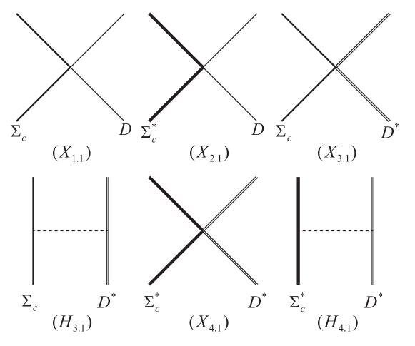
Figure 1: The leading order Feynman diagrams for the $\Sigma_{c}D$ ($X_{1.1}$), $\Sigma_{c}^{*}D$ ($X_{2.1}$), $\Sigma_{c}D^{*}$ ($X_{3.1}$, $H_{3.1}$), and $\Sigma_{c}^{*}D^{*}$ ($X_{4.1}$, $H_{4.1}$) systems. We use the thick line, heavy-thick line, thin line, double-thin line, and dashed line to denote the $\Sigma_{c}$, $\Sigma_{c}^{*}$, $D$, $D^{*}$, and $\pi$, respectively.

The explicit expressions of the contact potentials for the $\Sigma_{c}D$, $\Sigma_{c}^{*}D$, $\Sigma_{c}D^{*}$, and $\Sigma_{c}^{*}D^{*}$ systems are

$$\mathcal{V}_{\Sigma_{c}D}^{X_{1.1}} = -D_{a}+2\left(\mathbf{I}_{1}\cdot\mathbf{I}_{2}\right)E_{a},$$ (25)

$$\mathcal{V}_{\Sigma_{c}^{*}D}^{X_{2.1}} = -D_{a}+2\left(\mathbf{I}_{1}\cdot\mathbf{I}_{2}\right)E_{a},$$ (26)

$$\mathcal{V}^{X_{3.1}}_{\Sigma_{c}D^{*}} = -D_{a}+2\left(\mathbf{I}_{1}\cdot\mathbf{I}_{2}\right)E_{a}$$ (27)

$$+\frac{2}{3}\left[-D_{b}+2E_{b}\left(\mathbf{I}_{1}\cdot\mathbf{I}_{2}\right)\right]\bm{\sigma}\cdot\bm{T},$$

$$\mathcal{V}^{X_{4.1}}_{\Sigma_{c}^{*}D^{*}} = -D_{a}+2\left(\mathbf{I}_{1}\cdot\mathbf{I}_{2}\right)E_{a}$$ (28)

$$+\left[-D_{b}+2E_{b}\left(\mathbf{I}_{1}\cdot\mathbf{I}_{2}\right)\right]\bm{\sigma}_{rs}\cdot\bm{T}.$$

where $\mathbf{I}_{1}$ and $\mathbf{I}_{2}$ are the isospin operators of the $\Sigma_{c}^{(*)}$ and $D^{(*)}$, respectively. The matrix elements of $\mathbf{I}_{1}\cdot\mathbf{I}_{2}$ can be obtained via

$$\left\langle\mathbf{I}_{1}\cdot\mathbf{I}_{2}\right\rangle=\frac{1}{2}\left[I(I+1)-I_{1}(I_{1}+1)-I_{2}(I_{2}+1)\right],$$ (29)

where $I$ is the total isospin of the $\Sigma_{c}^{(*)}D^{(*)}$ systems. The cross product of the final and initial polarization vectors for $D^{*}$ mesons ($\bm{\varepsilon}^{\dagger}$ and $\bm{\varepsilon}$, respectively) is given in terms of $\bm{T}$ operator

$$-i\bm{T}=\bm{\varepsilon}^{\dagger}\times\bm{\varepsilon}.$$ (30)

where the spin operator $\bm{S}_{v}$ of the $D^{*}$ meson can be related to the $\bm{T}$ operator via

$$\bm{S}_{v}=-\bm{T}.$$ (31)

The spin operators $\bm{S}_{s}$ of $\Sigma_{c}$ and $\bm{S}_{rs}$ of $\Sigma_{c}^{\ast}$ are related to the Pauli matrix $\bm{\sigma}$ and $\bm{\sigma}_{rs}$ via

$$\bm{S}_{s}=\frac{1}{2}\bm{\sigma},\qquad\bm{S}_{rs}=\frac{3}{2}\bm{\sigma}_{rs}.$$ (32)

Then the matrix elements of the $\bm{\sigma}\cdot\bm{T}$ and $\bm{\sigma}_{rs}\cdot\bm{T}$ can be obtained from Eqs. (31)-(32) by

$$\bm{\sigma}\cdot\bm{T} = -2\bm{S}_{1}\cdot\bm{S}_{2}$$

$$= -\left[S(S+1)-S_{1}(S_{1}+1)-S_{2}(S_{2}+1)\right],$$

$$\bm{\sigma}_{rs}\cdot\bm{T} = -\frac{2}{3}\bm{S}_{1}\cdot\bm{S}_{2}$$

$$= -\frac{1}{3}\left[S(S+1)-S_{1}(S_{1}+1)-S_{2}(S_{2}+1)\right].$$

where $\bm{S}_{1}\equiv\bm{S}_{s}(\bm{S}_{rs})$ and $\bm{S}_{2}\equiv\bm{S}_{v}$ denote the spin operators of the $\Sigma^{(*)}_{c}$ baryon and $D^{*}$ meson, respectively.

The one-pion-exchange diagrams for the $\Sigma_{c}D^{*}$ and $\Sigma_{c}^{*}D^{*}$ systems are depicted in graphs ($H_{3.1}$) and ($H_{4.1}$) of Fig. 1. The corresponding effective potentials read

$$\mathcal{V}_{\Sigma_{c}D^{*}}^{H_{3.1}} = \left(\mathbf{I}_{1}\cdot\mathbf{I}_{2}\right)\frac{gg_{1}}{2f_{\pi}^{2}}\frac{\left(\bm{q}\cdot\bm{\sigma}\right)\left(\bm{q}\cdot\bm{T}\right)}{\bm{q}^{2}+m_{\pi}^{2}},$$ (34)

$$\mathcal{V}_{\Sigma_{c}^{*}D^{*}}^{H_{4.1}} = -\left(\mathbf{I}_{1}\cdot\mathbf{I}_{2}\right)\frac{gg_{5}}{2f_{\pi}^{2}}\frac{\left(\bm{q}\cdot\bm{\sigma}_{rs}\right)\left(\bm{q}\cdot\bm{T}\right)}{\bm{q}^{2}+m_{\pi}^{2}}.$$ (35)

One can notice that there is a minus sign between the one-pion-exchange amplitudes of the $\Sigma_{c}^{(*)}D^{*}$ and $\Sigma_{c}^{(*)}\bar{D}^{*}$ systems Wang:2019ato . This minus sign comes from the $G$-parity transformation between the ($\bar{D}^{(*)0}$, $D^{(*)-}$) and ($D^{(*)+}$, $D^{(*)0}$) doublets.

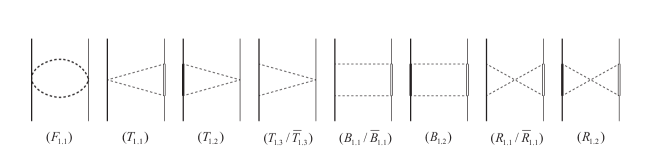
Figure 2: Two-pion-exchange diagrams that account for the effective potentials of the $\Sigma_{c}D$ system at next-to-leading order. These diagrams include the football diagram ($F_{1.1}$), triangle diagrams ($T_{1.i}/\bar{T}_{1.i}$), box diagrams ($B_{1.i}/\bar{B}_{1.i}$), and crossed box diagrams ($R_{1.i}/\bar{R}_{1.i}$). The $\bar{T}_{1.3}$, $\bar{B}_{1.1}$, and $\bar{R}_{1.1}$ denote the diagrams with $\Lambda_{c}$ as the intermediate state. The notations are the same as those in Fig. 1.

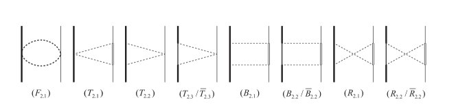
Figure 3: Two-pion-exchange diagrams for the $\Sigma^{*}_{c}D$ system. The notations are the same as those in Fig. 2.

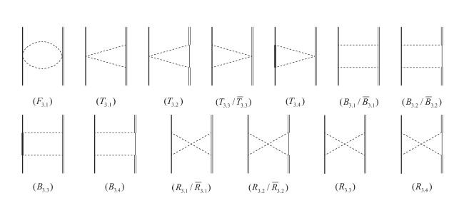
Figure 4: Two-pion-exchange diagrams for the $\Sigma_{c}D^{*}$ system. The notations are the same as those in Fig. 2.

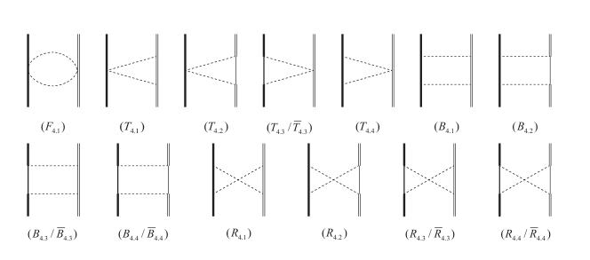
Figure 5: Two-pion-exchange diagrams for the $\Sigma^{*}_{c}D^{\ast}$ system. The notations are the same as those in Fig. 2.

The two-pion-exchange diagrams for the $\Sigma_{c}D$, $\Sigma_{c}^{*}D$, $\Sigma_{c}D^{*}$, and $\Sigma_{c}^{*}D^{*}$ systems are illustrated in Figs. 2, 3, 4, and 5, respectively. The analytical results for the football diagrams ($F_{i.j}$), triangle diagrams ($T_{i.j}$), box diagrams ($B_{i.j}$), and crossed box diagrams ($R_{i.j}$) generally have the following forms,

$$\mathcal{V}_{\rm{sys}}^{F_{i.j}} = \left(\mathbf{I}_{1}\cdot\mathbf{I}_{2}\right)\frac{1}{f_{\pi}^{4}}J_{22}^{F}(m_{\pi},q),$$ (36)

$$\mathcal{V}_{\rm{sys}}^{T_{i,j}} = \left(\mathbf{I}_{1}\cdot\mathbf{I}_{2}\right)\frac{\mathcal{C}_{\rm{sys}}^{T_{i.j}}}{f_{\pi}^{4}}\left[-\bm{q}^{2}\mathcal{C}_{1}^{T_{i.j}}\left(J_{24}^{T}+J_{33}^{T}\right)\right.$$ (37)

$$\left.+\mathcal{C}_{2}^{T_{i.j}}J_{34}^{T}\right]\left(m_{\pi},\mathcal{E}^{T_{i.j}},q\right),$$

$$\mathcal{V}_{\rm{sys}}^{B_{i.j}} = \left(1-\mathbf{I}_{1}\cdot\mathbf{I}_{2}\right)\frac{\mathcal{C}_{\rm{sys}}^{B_{i.j}}}{f_{\pi}^{4}}\left[-\bm{q}^{2}\mathcal{C}_{1}^{B_{i.j}}J_{21}^{B}\right.$$ (38)

$$+\bm{q}^{4}\mathcal{C}_{2}^{B_{i.j}}(J_{22}^{B}+2J_{32}^{B}+J_{43}^{B})-\bm{q}^{2}\mathcal{C}_{3}^{B_{i.j}}(J_{31}^{B}$$

$$+J_{42}^{B})\left.+\mathcal{C}_{4}^{B_{i.j}}J_{41}^{B}\right]\left(m_{\pi},\mathcal{E}_{1}^{B_{i.j}},\mathcal{E}^{B_{i.j}}_{2},q\right),$$

$$\mathcal{V}_{\rm{sys}}^{R_{i.j}} = \left(1+\mathbf{I}_{1}\cdot\mathbf{I}_{2}\right)\frac{\mathcal{C}_{\rm{sys}}^{R_{i.j}}}{f_{\pi}^{4}}\left[-\bm{q}^{2}\mathcal{C}_{1}^{R_{i.j}}J_{21}^{R}\right.$$ (39)

$$+\bm{q}^{4}\mathcal{C}_{2}^{R_{i.j}}\left(J_{22}^{R}+2J_{32}^{R}+J_{43}^{R}\right)-\bm{q}^{2}\mathcal{C}_{3}^{R_{i.j}}(J_{31}^{R}$$

$$+J_{42}^{R})\left.+\mathcal{C}_{4}^{R_{i.j}}J_{41}^{R}\right]\left(m_{\pi},\mathcal{E}_{1}^{R_{i.j}},\mathcal{E}^{R_{i.j}}_{2},q\right),$$

where the subscript “sys” denotes the corresponding $\Sigma_{c}^{(*)}D^{(*)}$ system. The superscripts $F_{i.j}$, $T_{i.j}$, $B_{i.j}$, and $R_{i.j}$ are the labels of Feynman diagrams illstrated in Figs. 2-5. The $J_{x}^{T}$, $J_{x}^{B}$, $J_{x}^{R}$ are scalar loop functions defined in Appendix A of Ref. Wang:2019ato . $\mathcal{E}^{T_{i.j}}$, $\mathcal{E}_{1(2)}^{B_{i.j}}$, $\mathcal{E}^{R_{i.j}}_{1(2)}$ are the residual energies.

In Ref. Wang:2019ato , we found the contributions of $\Lambda_{c}$ in the loops of two-pion-exchange diagrams have considerable corrections to the effective potentials. Thus, in this work, we also consider the contributions from intermediate $\Lambda_{c}$ state. The general expressions for the corresponding triangle diagrams ($\bar{T}_{i.j}$), box diagrams ($\bar{B}_{i.j}$), and crossed box diagrams ($\bar{R}_{i.j}$) read

$$\mathcal{V}^{\bar{T}_{i.j}}_{\rm{sys}} = \left(\mathbf{I}_{1}\cdot\mathbf{I}_{2}\right)\frac{C_{\rm{sys}}^{\bar{T}_{i.j}}}{f_{\pi}^{4}}\left[-\bm{q}^{2}\mathcal{C}_{1}^{\bar{T}_{i.j}}\left(J_{24}^{T}+J_{33}^{T}\right)\right.$$ (40)

$$\left.+\mathcal{C}_{2}^{\bar{T}_{i.j}}\right]\left(m_{\pi},\mathcal{E}^{\bar{T}_{i.j}},q\right),$$

$$\mathcal{V}_{\rm{sys}}^{\bar{B}_{i.j}} = \left(1-2\mathbf{I}_{1}\cdot\mathbf{I}_{2}\right)\frac{\mathcal{C}_{\rm{sys}}^{\bar{B}_{i.j}}}{f_{\pi}^{4}}\left[-\bm{q}^{2}\mathcal{C}_{1}^{\bar{B}_{i.j}}J_{21}^{B}\right.$$ (41)

$$+\bm{q}^{4}\mathcal{C}_{2}^{\bar{B}_{i.j}}\left(J_{22}^{B}+2J_{32}^{B}+J_{43}^{B}\right)-\bm{q}^{2}\mathcal{C}_{3}^{\bar{B}_{i.j}}(J^{B}_{31}$$

$$+J_{42}^{B})\left.+\mathcal{C}_{4}^{\bar{B}_{i.j}}J_{41}^{B}\right]\left(m_{\pi},\mathcal{E}_{1}^{\bar{B}_{i.j}},\mathcal{E}_{2}^{\bar{B}_{i.j}},q\right),$$

$$\mathcal{V}_{\rm{sys}}^{\bar{R}_{i.j}} = \left(1+2\mathbf{I}_{1}\cdot\mathbf{I}_{2}\right)\frac{\mathcal{C}_{\rm{sys}}^{\bar{R}_{i.j}}}{f_{\pi}^{4}}\left[-\bm{q}^{2}\mathcal{C}_{1}^{\bar{R}_{i.j}}J_{21}^{R}\right.$$ (42)

$$+\bm{q}^{4}\mathcal{C}_{2}^{\bar{R}_{i.j}}\left(J_{22}^{R}+2J_{32}^{R}+J_{43}^{R}\right)-\bm{q}^{2}\mathcal{C}_{3}^{\bar{R}_{i.j}}(J^{R}_{31}$$

$$+J_{42}^{R})\left.+\mathcal{C}_{4}^{\bar{R}_{i.j}}J_{41}^{R}\right]\left(m_{\pi},\mathcal{E}_{1}^{\bar{R}_{i.j}},\mathcal{E}_{2}^{\bar{R}_{i.j}},q\right),$$

One can see Appendix A for the explicit values of the coefficients defined in Eqs. (37)-(42).

We notice the expressions of the two-pion-exchange diagrams for the $\Sigma_{c}^{(*)}D^{(*)}$ systems are identical to those of the $\Sigma_{c}^{(*)}\bar{D}^{(*)}$ systems Wang:2019ato . This interesting results can be easily understood as follows: the differences between the two-pion-exchange amplitudes of the $\Sigma_{c}^{(*)}D^{(*)}$ and $\Sigma_{c}^{(*)}\bar{D}^{(*)}$ systems are completely caused by the pionic coupling of the charmed and anti-charmed mesons. As mentioned before, the one-pion vertices [from the $u_{\mu}$ in Eq. (2)] between the charmed and anti-charmed mesons have a minus sign difference, but they appear in pairs in the two-pion-exchange diagrams. Besides, the two-pion vertices [from the $\Gamma_{\mu}$ in Eq. (2)] is invariant under the $G$-parity transformation.

We have subtracted the 2PR contributions of the box diagrams in our calculations. This can be achieved by the principal-value integral method proposed in Ref. Wang:2019ato , in which a detailed derivation is presented in the Appendix B.

III Numerical results and discussions

To get the numerical results, we need to determine the four LECs defined in Eq. (21). At present, there are no experimental data or lattice QCD simulations for the possible $P_{cc}$ states. In Refs. Wang:2020dhf ; Wang:2019nvm ; Meng:2019nzy , we proposed to bridge the LECs determined from the $NN$ ($N\bar{N}$) scattering data to the unknown LECs of the di-hadron systems via a quark level contact Lagrangian. In this work, we apply this approach to estimate the contributions of the contact terms for the $\Sigma_{c}^{(*)}D^{(*)}$ systems, likewise. Then we search for binding solutions via solving the Schrödinger equation and discuss the numerical results.

III.1 Determining the LECs of the $\Sigma_{c}^{(*)}D^{(*)}$ systems

It is assumed that the contact terms are mimicked by exchanging heavy mesons through the $S$-wave interaction Wang:2020dhf ; Wang:2019nvm ; Meng:2019nzy , in which a general quark-level Lagrangian is constructed as

$$\mathcal{L}=g_{s}\bar{q}\mathcal{S}q+g_{a}\bar{q}\gamma_{\mu}\gamma^{5}\mathcal{A}^{\mu}q,$$ (43)

where $q=(u,d)$, $c_{s}$ and $c_{t}$ are two independent coupling constants. The fictitious scalar ($\mathcal{S}$) and axial-vector ($\mathcal{A}^{\mu}$) fields with positive parity are introduced to account for the central potential and spin-spin interaction, respectively. From Eq. (43), the $q\bar{q}$ contact potential is obtained as

$$V_{q\bar{q}}=c_{s}\left(1-3\bm{\tau}_{1}\cdot\bm{\tau}_{2}\right)+c_{t}\left(1-3\bm{\tau}_{1}\cdot\bm{\tau}_{2}\right)\bm{\sigma}_{1}\cdot\bm{\sigma}_{2}.$$ (44)

In Table 1, we present the quark-level matrix elements of the operators related to the contact potentials.

Table 1: The quark-level matrix elements of two-body interaction operators $\mathcal{O}_{ij}$ for the $N\bar{N}$ and $\Sigma_{c}D^{*}$ systems.

$\mathcal{O}_{ij}$	$\bm{1}_{ij}$	$\bm{\tau}_{i}\cdot\bm{\tau}_{j}$	$\bm{\sigma}_{i}\cdot\bm{\sigma}_{j}$	$\left(\bm{\tau}_{i}\cdot\bm{\tau}_{j}\right)\left(\bm{\sigma}_{i}\cdot\bm{\sigma}_{j}\right)$
$\left[N\bar{N}\right]^{I=1}_{J=1}$	9	1	1	$\frac{25}{9}$
$\left[N\bar{N}\right]^{I=1}_{J=0}$	9	1	-3	-$\frac{25}{3}$
$\left[N\bar{N}\right]^{I=0}_{J=1}$	9	-3	1	-$\frac{25}{3}$
$\left[N\bar{N}\right]^{I=0}_{J=0}$	9	-3	-3	25
$\left[\Sigma_{c}D^{*}\right]_{J=\frac{3}{2}}^{I=\frac{3}{2}}$	2	2	$\frac{4}{3}$	$\frac{4}{3}$

Based on the Lagrangian in Eq. (43) and the matrix elements in Table 1, the authors of Ref. Wang:2020dhf derived the contact potential of the $N\bar{N}$ system with quantum numbers $I=1$ and ${}^{2S+1}L_{J}=^{3}S_{1}$,

$$V_{N\bar{N}}^{{}^{3}S_{1}} = \left\langle N\bar{N}\left|V_{q\bar{q}}\right|N\bar{N}\right\rangle=6c_{s}-\frac{22}{3}c_{t}.$$ (45)

One can as well as obtain the contact potentials of the $[N\bar{N}]_{J=0}^{I=1}$, $[N\bar{N}]_{J=1}^{I=0}$, and $[N\bar{N}]_{J=0}^{I=0}$ systems, accordingly.

Similarly, the $\Sigma_{c}D^{*}$ contact potential can be obtained from Eq. (44) and Table 1 as

$$V_{\Sigma_{c}D^{*}} = 2c_{s}-12c_{s}\mathbf{I}_{1}\cdot\mathbf{I}_{2}-\frac{4}{3}c_{t}\bm{\sigma}\cdot\bm{T}$$ (46)

$$+8c_{t}\left(\mathbf{I}_{1}\cdot\mathbf{I}_{2}\right)\left(\bm{\sigma}\cdot\bm{T}\right).$$

Comparing Eq. (27) with Eq. (46) we get

$$D_{a}=-2c_{s},\quad E_{a}=-6c_{s},\quad D_{b}=2c_{t},\quad E_{b}=6c_{t}.$$

In Ref. Kang:2013uia , based on the $N\bar{N}$ scattering data, the LECs for the $I=0$ ($J=0,1$) and $I=1$ ($J=0,1$) $N\bar{N}$ systems are fitted. With the LECs of these four $N\bar{N}$ systems, we obtain six sets of solutions for the $c_{s}$ and $c_{t}$. Among them, four sets of $c_{s}$ and $c_{t}$ are consistent with each other in sizes and signs:

• Set 1: $c_{s}=-5.84$ GeV^-2,     $c_{t}=2.50$ GeV^-2;

• Set 2: $c_{s}=-8.10$ GeV^-2,     $c_{t}=0.65$ GeV^-2;

• Set 3: $c_{s}=-8.25$ GeV^-2,     $c_{t}=0.52$ GeV^-2;

• Set 4: $c_{s}=-7.71$ GeV^-2,     $c_{t}=0.38$ GeV^-2.

The remaining two sets of solutions either have the different signs or are too large, leading to unstable numerical results in our calculations.

When checking the above four sets of LECs, we notice that the $c_{s}$ value in Set 1 is smaller than those of other sets, the input with $c_{s}$ in Set 1 will lead to relatively small central potentials. On the contrary, the value of $c_{t}$ in Set 1 is larger than those of other sets, the spin-spin corrections would be important with this set of LECs. This is the first case we want to discuss, we label this set of LECs solution as Case 1. The LECs in Set 2 have been successfully applied to study the interactions of the $D^{(*)}N$ systems Wang:2020dhf , the small value of $c_{t}$ shows that with this set of solution, the spin-spin interaction serves as the perturbation to the $D^{(*)}N$ multiplets. The LECs in Sets 3 and 4 are very close to that of Set 2, and they give very similar results. Thus, we will use the LECs in Set 2 as our Case 2. In addition, we also use the least square method to fit a best solution from these four sets of LECs, the solution are obtained as

$$c_{s}=-7.46\rm{GeV}^{-2},\qquad c_{t}=1.02\rm{GeV}^{-2}.$$ (48)

we label this set of LECs as the Case 3.

III.2 Numerical results of the effective potentials

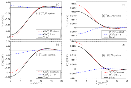
Figure 6: The effective potentials for the $[\Sigma^{(*)}_{c}D]^{I=1/2}_{J}$ systems. Their $I(J^{P})$ numbers are illustrated in each subfigure. The red dashed line and blue dot-dashed line denote the effective potentials from the contact term and two-pion-exchange, respectively. The black solid line denote the total effective potential for each system.

We use the LECs in Case 3 to present the effective potentials of all the $\Sigma_{c}^{(*)}D^{(*)}$ systems. In Fig. 6, we plot the effective potentials of the $\Sigma_{c}D$ and $\Sigma_{c}^{*}D$ systems. The contact terms of the $\Sigma_{c}D$ and $\Sigma_{c}^{*}D$ are the same in the heavy quark limit, which can be checked from the line shapes of the contact effective potentials in Fig. 6.

For the $[\Sigma_{c}D]^{I=1/2}_{J=1/2}$ system, the two-pion-exchange interaction provides a weakly repulsive force. The contact interaction provides a strong attractive force, which is also true for the $[\Sigma^{*}_{c}D]^{I=1/2}_{J=3/2}$ system. In the $[\Sigma^{*}_{c}D]^{I=1/2}_{J=3/2}$ system, the two-pion-exchange interaction provides a weakly attractive potential and forms a deeply bound $[\Sigma^{*}_{c}D]^{I=1/2}_{J=3/2}$ state together with the strong attractive contact term.

From the right panel of Fig. 6, we can see that the two-pion-exchange interactions provide considerable attractive force in the $[\Sigma^{(*)}_{c}D]^{I=3/2}_{J}$ systems. However, for the $I=3/2$ case, the contact terms provide strong repulsive forces and the total effective potentials are repulsive, i.e., we can not find any bound states. This is also true for the $[\Sigma^{(*)}_{c}D^{*}]^{I=3/2}_{J}$ systems. Thus, in the following, we only discuss the $\Sigma_{c}^{(*)}D^{(*)}$ systems with $I=1/2$.

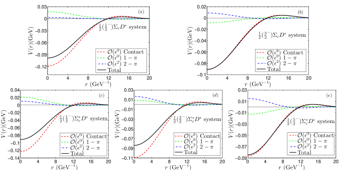
Figure 7: The effective potentials for the $[\Sigma^{(*)}_{c}D^{*}]^{I=1/2}_{J}$ systems. Their $I(J^{P})$ numbers are illustrated in each subfigure. The red dashed line, green dashed line and blue dot-dashed line denote the effective potentials from the contact term, one-pion- and two-pion-exchange interactions, respectively. The black solid line denote the total effective potential for each system.

In Fig. 7, we present the effective potentials of the $\Sigma_{c}^{(*)}D^{*}$ systems. From Fig. 7, we can see that in the $[\Sigma_{c}D^{*}]_{J}^{I=1/2}$ and $[\Sigma_{c}^{*}D^{*}]_{J}^{I=1/2}$ systems, the contact terms provide strong attractive force. The one-pion- and two-pion-exchange interactions supply very weak repulsive forces in the $[\Sigma_{c}D^{*}]_{J=1/2}^{I=1/2}$, $[\Sigma^{*}_{c}D^{*}]_{J=1/2(3/2)}^{I=1/2}$ systems. For the $[\Sigma_{c}D^{*}]_{J=3/2}^{I=1/2}$ and $[\Sigma_{c}^{*}D^{*}]_{J=5/2}^{I=1/2}$ systems, the one-pion- and two-pion-exchange potentials supply comparable attractive and repulsive forces, respectively. Thus, the total effective potentials for these two systems are nearly equivalent to their contact potentials.

Our calculation shows that the contact terms are important to the $[\Sigma_{c}^{(*)}D^{(*)}]^{I=1/2}_{J}$ systems. In our framework, the fictitious scalar mesons account for the mainly attractive interactions in the $[\Sigma_{c}^{(*)}D^{(*)}]^{I=1/2}_{J}$ systems, and the exchange of axial-vector mesons result in mass splittings in spin multiplets. In Eq. (43), the $c_{s}$ and $c_{t}$ are related to the strength of the scalar-exchange and axial-vector-exchange forces, respectively. From Table 2, we notice that the axial-vector-exchange interactions which are related to the $c_{t}$ provide small corrections to the final effective potentials in Cases 2 and 3. However, in Case 1, we have $|c_{t}/c_{s}|=0.43$, this can be regarded as our upper limit of the $|c_{t}/c_{s}|$. The relatively small value of $c_{t}$ can be traced to the large masses of the axial-vector particles since their masses exceed $1$ GeV Zyla:2020zbs .

III.3 The binding energies of the $\Sigma_{c}^{(*)}D^{(*)}$ systems

Table 2: The binding energies, masses and root-mean-square radii for all the $[\Sigma_{c}^{(*)}D^{(*)}]^{I=1/2}_{J}$ systems. The subscript denotes the total angular momentum of this system. The adopted LECs in Cases 1, 2, and 3 are ($c_{s}=-5.84$, $c_{t}=2.50$) GeV^-2, ($c_{s}=-8.10$, $c_{t}=0.65$ ) GeV^-2, and ($c_{s}=-7.46$, $c_{t}=1.02$) GeV^-2, respectively.

		$\left[\Sigma_{c}D\right]_{\frac{1}{2}}$	$\left[\Sigma^{*}_{c}D\right]_{\frac{3}{2}}$	$\left[\Sigma_{c}D^{*}\right]_{\frac{1}{2}}$	$\left[\Sigma_{c}D^{*}\right]_{\frac{3}{2}}$	$\left[\Sigma_{c}^{*}D^{*}\right]_{\frac{1}{2}}$	$\left[\Sigma_{c}^{*}D^{*}\right]_{\frac{3}{2}}$	$\left[\Sigma_{c}^{*}D^{*}\right]_{\frac{5}{2}}$
Case 1	BE (MeV)	-15.4	-25.0	-31.8	-8.0	-32.8	-18.2	-3.5
	$R_{rms}$ (fm)	1.45	1.25	1.20	1.65	1.20	1.38	1.91
Case 2	BE (MeV)	-31.3	-42.9	-30.3	-31.7	-26.6	-25.4	-29.7
	$R_{rms}$ (fm)	1.23	1.11	1.22	1.20	1.26	1.27	1.22
Case 3	BE (MeV)	-26.5	-37.7	-29.1	-25.0	-26.4	-22.6	-22.2
	$R_{rms}$ (fm)	1.27	1.14	1.23	1.27	1.26	1.31	1.30

The binding energies, masses, and the root-mean-square radii in the above three cases are presented in Table 2. We find bound state solutions only for the $I=1/2$ channels. The $R_{rms}$ are about 1$-$2 fm for all the considered $\Sigma_{c}^{(*)}D^{(*)}$ systems, which are the typical sizes of the hadronic molecules. From Table 2, we can see that the binding of the $[\Sigma_{c}^{*}D]_{J=3/2}^{I=1/2}$ system is deeper than that of the $[\Sigma_{c}D]_{J=1/2}^{I=1/2}$ system. In the heavy quark limit, the $[\Sigma_{c}D]_{J=1/2}^{I=1/2}$ and $[\Sigma_{c}^{*}D]_{J=3/2}^{I=1/2}$ systems share the same contact term. Thus, the difference of the binding energy is from the contributions of the two-pion-exchange interactions. Besides, in Case 1, the $\Sigma_{c}^{(*)}D^{*}$ systems with lower total angular momentum $J$ are more compact. This situation is very similar to the $\Sigma_{c}^{(*)}\bar{D}^{*}$ systems Wang:2019ato . However, the results in Cases 2 and 3 show that the binding energies for the different $\Sigma_{c}^{(*)}D^{(*)}$ systems are comparable to each other, and they have very similar spatial sizes.

The parameters $c_{s}$ and $c_{t}$ are related to the central potentials and spin-spin interactions, respectively. In Case 1, $|c_{t}/c_{s}|=0.43$, the spin-spin corrections in contact terms have considerable contributions in the $\Sigma_{c}^{(*)}D^{*}$ systems [note that the spin-spin corrections do not contribute to the $\Sigma_{c}^{(*)}D$ systems, e.g., see Eqs. (25)-(26)]. The spin-spin corrections are much larger than the contributions from the one-pion-exchange and two-pion-exchange interactions. Thus, in Case 1, the mass splittings among different $[\Sigma_{c}^{(*)}D^{*}]_{J}^{I=1/2}$ systems are mainly caused by the corrections of the spin-spin interactions. The results obtained from the Cases 2 and 3 are close to each other. In contrast to Case 1, $|c_{t}/c_{s}|\approx 0.1$ in these two cases, i.e., the central potentials are dominant and the spin-spin potentials are small. The contributions from the spin-spin interactions are comparable to those of the one-pion-exchange and two-pion-exchange interactions. As shown in Table 2, in these two cases, the $\Sigma_{c}^{(*)}D^{*}$ systems with higher total angular momenta have deeper binding energies.

The results for the $\Sigma_{c}^{(*)}\bar{B}^{(*)}$, $\Sigma_{b}^{(*)}D^{(*)}$, and $\Sigma_{b}^{(*)}\bar{B}^{(*)}$ systems are given in Appendix B.

III.4 Possible decay patterns of the $\Sigma_{c}^{(*)}D^{(*)}$ molecules

The $P_{c}(4312)$, $P_{c}(4440)$, and $P_{c}(4457)$ are produced in the $\Lambda_{b}^{0}\rightarrow J/\psi K^{-}p$ decay process and reconstructed in the $J/\psi p$ channel Aaij:2019vzc . Similarly, the $P_{cs}(4459)$ is produced in the $\Xi_{b}^{-}\rightarrow J/\psi K^{-}\Lambda$ process and observed in the $J/\psi\Lambda$ invariant mass spectrum Aaij:2020gdg . In this subsection, we discuss the possible decay patterns of the $P_{cc}$ states. They may be considered as the reconstructive channels from the $pp$ collisions at LHCb.

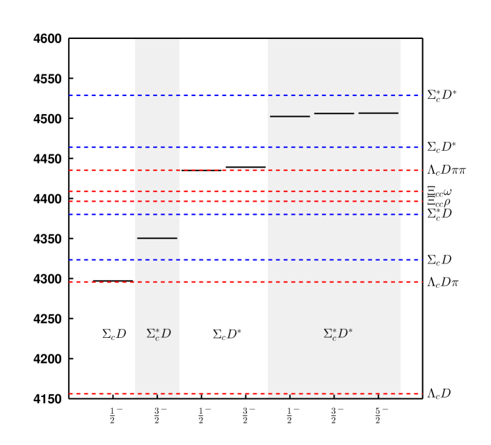
Figure 8: The mass spectrum of the $P_{cc}$ pentaquarks. The results are obtained using the LECs in Case 3. The black solid lines denote the $P_{cc}$ pentaquarks. The blue and red dotted lines denote the thresholds of the $\Sigma^{(*)}_{c}D^{(*)}$ and possible decay channels, respectively.

In Fig. 8, we present the mass spectrum of the $P_{cc}$ pentaquarks based on the inputs in Case 3, and some relevant thresholds. Due to the $cc$ pairs in the $P_{cc}$ pentaquarks, the decay behaviors of the $P_{cc}$ states are different from that of the hidden-charm pentaquarks. There exist two types of decay modes for the $P_{cc}$ states, i.e., the $(cqq)$-$(c\bar{q})$ and $(ccq)$-$(q\bar{q})$ modes. Note that the $\Lambda_{c}\pi$ and $D\pi$ are the dominant decay channels for the $\Sigma_{c}^{(*)}$ baryons and $D^{*}$ meson, respectively. For simplicity, we only consider the ground $\Lambda_{c}$, $D$, and $\pi$ as our decay final states in the first mode. From Fig. 8, we can see that the $P_{cc}(4296)$ state with $J^{P}=1/2^{-}$ is near the threshold of the $\Lambda_{c}D\pi$. Thus, it is very difficult for this state to decay into this three-body final state due to the small phase space. But the $P_{cc}(4296)$ can easily decay into $\Lambda_{c}D$ two-body final states. Further study on the branching ratio of this decay process is still needed. The $P_{cc}(4350)$ with $J^{P}=3/2^{-}$ can decay into the $\Lambda_{c}D\pi$ via the $S$-wave, while decaying into the $\Lambda_{c}D$ is $D$-wave suppressed. One can perform similar analyses for the other five $P_{cc}$ states.

Now we discuss the $(ccq)$-$(q\bar{q})$ decay mode, i.e., the $P_{cc}$ states decay into the ground $\Xi_{cc}$ baryon and a pseudoscalar or a vector meson. The threshold of $\Xi_{cc}\pi$ channel is about 3760 MeV, which is much lower than the $P_{cc}$ states and is not presented in Fig. 8. The predicted $P_{cc}$ states with $J^{P}=1/2^{-}$ can decay into this channel through $S$-wave, thus, this should be an important strong decay channels for the $J^{P}=1/2^{-}$ states due to the large phase spaces. The states that are composed of the $\Sigma^{(*)}_{c}$ and $D^{*}$ can also decay into the $\Xi_{cc}\omega$ and $\Xi_{cc}\rho$ final states. One can also extract the decay properties for the other $P_{cc}$ pentaquarks in Fig. 8.

IV Summary

Inspired by the recently observed $P_{c}$ Aaij:2019vzc and $P_{cs}$ Aaij:2020gdg pentaquarks, we perform a systematic study on the interactions of the $\Sigma_{c}^{(*)}D^{(*)}$ systems to explore the possible $P_{cc}$ states. We include the contact term, one-pion-exchange, and two-pion-exchange interactions within the framework of chiral effective field theory.

Due to $G$-parity transformation law, the expressions of the one-pion-exchange and two-pion-exchange effective potentials of the $\Sigma_{c}^{(*)}D^{(*)}$ systems are opposite and identical to those of the $\Sigma_{c}^{(*)}\bar{D}^{(*)}$ systems Wang:2019ato , respectively. With the LECs fitted from the $N\bar{N}$ scattering data, we obtain four sets of ($c_{s}$, $c_{t}$) parameters describing the contributions of the contact terms. We present three cases to study the binding energies of the $\Sigma_{c}^{(*)}D^{(*)}$ systems.

The mass spectrum of the $[\Sigma_{c}^{(*)}D^{(*)}]^{I=1/2}_{J}$ molecules depend on the values of the LECs. In Case 1, a relatively small central potential and a large spin-spin interaction are introduced. The obtained $P_{cc}$ mass spectrum is very similar to that of the $\Sigma_{c}^{(*)}\bar{D}^{(*)}$ systems. However, the mass spectra obtained in Cases 2 and 3 are different from that of the Case 1. Further experimental studies may help us to clarify the predicted mass spectra of the $\Sigma_{c}^{(*)}D^{(*)}$ systems in different cases.

We briefly discuss the strong decay behaviors of the $P_{cc}$ pentaquarks. The $(cqq)$-$(c\bar{q})$ and $(ccq)$-$(q\bar{q})$ are the two types of decay modes. Correspondingly, the $\Lambda_{c}D$, $\Lambda_{c}D\pi$, and $\Xi_{cc}\pi$ are expected to be important channels to search for these $[\Sigma_{c}^{(*)}D^{(*)}]^{I=1/2}_{J}$ molecules.

We also study the interactions of the $\Sigma_{c}^{(*)}\bar{B}^{(*)}$, $\Sigma_{b}^{(*)}D^{(*)}$, and $\Sigma_{b}^{(*)}\bar{B}^{(*)}$ to search for possible $P_{cb}$, $P_{bc}$, and $P_{bb}$ pentaquarks. The corresponding systems with $I=1/2$ can also form molecular states. In addition, among the studied systems, the binding becomes deeper when the reduced masses of the systems are heavier.

Appendix A Supplements for the two-pion-exchange expressions

In Sec. II.2, we present the general expressions for the football diagrams ($F_{i.j}$), triangle diagrams ($T_{i.j}$), ($\bar{T}_{i.j}$), box diagrams ($B_{i.j}$), ($\bar{B}_{i.j}$) and crossed box diagrams $(R_{i.j})$, ($\bar{R}_{i.j}$) in Eqs. (36)-(42). In this appendix, we give their explicit coefficients defined in Eqs. (36)-(42).

Specifically, we collect the coefficients $\mathcal{C}_{\rm{sys}}^{T_{i.j}}$ ($\mathcal{C}_{\rm{sys}}^{\bar{T}_{i.j}}$), $\mathcal{C}_{\rm{sys}}^{(B/R)_{i.j}}$ ($\mathcal{C}_{\rm{sys}}^{(\bar{B}/\bar{R})_{i.j}}$) in Table 3, the coefficients of triangle diagrams $\mathcal{C}_{m}^{T_{i.j}}$ ($\mathcal{C}_{m}^{\bar{T}_{i.j}}$) and $\mathcal{E}^{T_{i.j}}$ ($\mathcal{E}^{\bar{T}_{i.j}}$) in Table 4, the coefficients of box and crossed box diagrams $\mathcal{C}_{m}^{B_{i.j}}$, $\mathcal{C}_{m}^{R_{i.j}}$ and $\mathcal{E}_{n}^{(B/R)_{i.j}}$ in Table 5, and the coefficients of box and crossed box diagrams $\mathcal{C}_{m}^{\bar{B}_{i.j}}$, $\mathcal{C}_{m}^{\bar{R}_{i.j}}$ and $\mathcal{E}_{n}^{(\bar{B}/\bar{R})_{i.j}}$ in Table 6.

Table 3: The coefficients $\mathcal{C}_{\rm{sys}}^{T_{i.j}}$ ($\mathcal{C}_{\rm{sys}}^{\bar{T}_{i.j}}$), $\mathcal{C}_{\rm{sys}}^{(B/R)_{i.j}}$ ($\mathcal{C}_{\rm{sys}}^{(\bar{B}/\bar{R})_{i.j}}$) defined in Eqs. (37)-(42). The superscripts denote the corresponding diagrams illustrated in Figs. 2, 3, 4, and 5, respectively.

$\mathcal{C}_{\rm{sys}}^{T_{i.1}}$

$\mathcal{C}_{\rm{sys}}^{T_{i.2}}$

$\mathcal{C}_{\rm{sys}}^{T_{i.3}}$

$\mathcal{C}_{\rm{sys}}^{T_{i.4}}$

$\mathcal{C}_{\rm{sys}}^{(B/R)_{i.1}}$

$\mathcal{C}_{\rm{sys}}^{(B/R)_{i.2}}$

$\mathcal{C}_{\rm{sys}}^{(B/R)_{i.3}}$

$\mathcal{C}_{\rm{sys}}^{(B/R)_{i.4}}$

$\mathcal{C}_{\rm{sys}}^{\bar{T}_{i.3}}$

$\mathcal{C}_{\rm{sys}}^{(\bar{B}/\bar{R})_{i.1}}$

$\mathcal{C}_{\rm{sys}}^{(\bar{B}/\bar{R})_{i.2}}$

$\mathcal{C}_{\rm{sys}}^{(\bar{B}/\bar{R})_{i.3}}$

$\mathcal{C}_{\rm{sys}}^{(\bar{B}/\bar{R})_{i.4}}$

$\Sigma_{c}D$

$g^{2}$

$\frac{g_{3}^{2}}{4}$

$\frac{g_{1}^{2}}{4}$

-

$\frac{g^{2}g_{1}^{2}}{8}$

$\frac{g^{2}g_{3}^{2}}{8}$

-

-

$\frac{g_{2}^{2}}{2}$

$\frac{g^{2}g_{2}^{2}}{8}$

-

-

-

$\Sigma_{c}^{*}D$

$g^{2}$

$\frac{5g_{5}^{2}}{36}$

$\frac{g_{3}^{2}}{4}$

-

$\frac{5g^{2}g_{5}^{2}}{72}$

$\frac{g^{2}g_{3}^{2}}{8}$

-

-

$\frac{g_{4}^{2}}{2}$

-

$\frac{g^{2}g_{4}^{2}}{8}$

-

-

$\Sigma_{c}D^{*}$

$g^{2}$

$g^{2}$

$\frac{g_{1}^{2}}{4}$

$\frac{g_{3}^{2}}{4}$

$\frac{g^{2}g_{1}^{2}}{8}$

$\frac{g^{2}g_{1}^{2}}{8}$

$\frac{g^{2}g_{3}^{2}}{8}$

$\frac{g^{2}g_{3}^{2}}{24}$

$\frac{g_{2}^{2}}{2}$

$\frac{g^{2}g_{2}^{2}}{8}$

$\frac{g^{2}g_{2}^{2}}{8}$

-

-

$\Sigma_{c}^{*}D^{*}$

$g^{2}$

$g^{2}$

$\frac{g_{3}^{2}}{4}$

$\frac{5g_{5}^{2}}{36}$

$\frac{g^{2}g_{5}^{2}}{24}$

$\frac{g^{2}g_{5}^{2}}{24}$

$\frac{g^{2}g_{3}^{2}}{32}$

$\frac{g^{2}g_{3}^{2}}{32}$

$\frac{g_{4}^{2}}{2}$

-

-

$\frac{g^{2}g_{4}^{2}}{32}$

$\frac{g^{2}g_{4}^{2}}{32}$

Table 4: The coefficients $\mathcal{C}_{m}^{T_{i.j}}$ ($\mathcal{C}_{m}^{\bar{T}_{i.j}}$) and $\mathcal{E}^{T_{i.j}}$ ($\mathcal{E}^{\bar{T}_{i.j}}$) defined in Eqs. (37) and (40). The superscript denotes the corresponding diagrams illustrated in Figs. 2, 3, 4, and 5, respectively.

	$\mathcal{C}_{1}^{T_{i.1}}$	$\mathcal{C}_{2}^{T_{i.1}}$	$\mathcal{E}^{T_{i.1}}$	$\mathcal{C}_{1}^{T_{i.2}}$	$\mathcal{C}_{2}^{T_{i.2}}$	$\mathcal{E}^{T_{i.2}}$	$\mathcal{C}_{1}^{T_{i.3}}$	$\mathcal{C}_{2}^{T_{i.3}}$	$\mathcal{E}^{T_{i.3}}$	$\mathcal{C}_{1}^{T_{i.4}}$	$\mathcal{C}_{2}^{T_{i.4}}$	$\mathcal{E}^{T_{i.4}}$	$\mathcal{C}_{1}^{\bar{T}_{i.3}}$	$\mathcal{C}_{2}^{\bar{T}_{i.3}}$	$\mathcal{E}^{\bar{T}_{i.3}}$
$\Sigma_{c}D$	1	3	$\mathcal{E}-\delta_{b}$	$\frac{2}{3}$	2	$\mathcal{E}-\delta_{a}$	1	3	$\mathcal{E}$	-	-	-	1	3	$\mathcal{E}+\delta_{c}$
$\Sigma_{c}^{*}D$	1	3	$\mathcal{E}-\delta_{b}$	1	3	$\mathcal{E}$	$\frac{1}{3}$	1	$\mathcal{E}+\delta_{a}$	-	-	-	$\frac{1}{3}$	1	$\mathcal{E}+\delta_{d}$
$\Sigma_{c}D^{*}$	$\frac{2}{3}$	2	$\mathcal{E}$	$\frac{1}{3}$	1	$\mathcal{E}+\delta_{b}$	1	3	$\mathcal{E}$	$\frac{2}{3}$	2	$\mathcal{E}-\delta_{a}$	1	3	$\mathcal{E}+\delta_{c}$
$\Sigma_{c}^{*}D^{*}$	$\frac{2}{3}$	2	$\mathcal{E}$	$\frac{1}{3}$	1	$\mathcal{E}+\delta_{b}$	$\frac{1}{3}$	1	$\mathcal{E}+\delta_{a}$	1	3	$\mathcal{E}$	$\frac{1}{3}$	1	$\mathcal{E}+\delta_{d}$

Table 5: The coefficients $\mathcal{C}_{m}^{B_{i.j}}$, $\mathcal{C}_{m}^{R_{i.j}}$ and $\mathcal{E}_{n}^{(B/R)_{i.j}}$ defined in Eqs. (38) and (39). The superscripts denote the corresponding diagrams illustrated in Figs. 2, 3, 4, and 5, respectively.

	$\mathcal{C}_{1}^{B_{i.1}}$	$\mathcal{C}_{1}^{R_{i.1}}$	$\mathcal{C}_{2}^{(B/R)_{i.1}}$	$\mathcal{C}_{3}^{(B/R)_{i.1}}$	$\mathcal{C}_{4}^{(B/R)_{i.1}}$	$\mathcal{E}_{1}^{(B/R)_{i.1}}$	$\mathcal{E}_{2}^{(B/R)_{i.1}}$
$\Sigma_{c}D$	1	1	1	10	15	$\mathcal{E}$	$\mathcal{E}-\delta_{b}$
$\Sigma_{c}^{*}D$	1	1	1	10	15	$\mathcal{E}$	$\mathcal{E}-\delta_{b}$
$\Sigma_{c}D^{*}$	$\frac{2+A}{3}$	$\frac{2-A}{3}$	$\frac{2}{3}$	$\frac{20}{3}$	10	$\mathcal{E}$	$\mathcal{E}$
$\Sigma^{*}_{c}D^{*}$	$B^{2}$	$\frac{3B^{2}-2B}{3}$	$\frac{10}{9}$	$\frac{20+12B^{2}-4B}{3}$	$10+6B^{2}-2B$	$\mathcal{E}$	$\mathcal{E}$
	$\mathcal{C}_{1}^{B_{i.2}}$	$\mathcal{C}_{1}^{R_{i.2}}$	$\mathcal{C}_{2}^{(B/R)_{i.2}}$	$\mathcal{C}_{3}^{(B/R)_{i.2}}$	$\mathcal{C}_{4}^{(B/R)_{i.2}}$	$\mathcal{E}_{1}^{(B/R)_{i.2}}$	$\mathcal{E}_{1}^{(B/R)_{i.2}}$
$\Sigma_{c}D$	$\frac{2}{3}$	$\frac{2}{3}$	$\frac{2}{3}$	$\frac{20}{3}$	10	$\mathcal{E}-\delta_{a}$	$\mathcal{E}-\delta_{b}$
$\Sigma_{c}^{*}D$	$\frac{1}{3}$	$\frac{1}{3}$	$\frac{1}{3}$	$\frac{10}{3}$	5	$\mathcal{E}+\delta_{a}$	$\mathcal{E}-\delta_{b}$
$\Sigma_{c}D^{*}$	$\frac{1+A}{3}$	$\frac{1-A}{3}$	$\frac{1}{3}$	$\frac{10}{3}$	5	$\mathcal{E}$	$\mathcal{E}+\delta_{b}$
$\Sigma^{*}_{c}D^{*}$	$\frac{5-3B^{2}+2B}{3}$	$\frac{5-3B^{2}}{3}$	$\frac{5}{9}$	$\frac{15-6B^{2}+2B}{3}$	$15-6B^{2}+2B$	$\mathcal{E}$	$\mathcal{E}+\delta_{b}$
	$\mathcal{C}_{1}^{B_{i.3}}$	$\mathcal{C}_{1}^{R_{i.3}}$	$\mathcal{C}_{2}^{(B/R)_{i.3}}$	$\mathcal{C}_{3}^{(B/R)_{i.3}}$	$\mathcal{C}_{4}^{(B/R)_{i.3}}$	$\mathcal{E}_{1}^{(B/R)_{i.3}}$	$\mathcal{E}_{1}^{(B/R)_{i.3}}$
$\Sigma_{c}D^{*}$	$\frac{4-A}{9}$	$\frac{4+A}{9}$	$\frac{4}{9}$	$\frac{40}{9}$	$\frac{20}{3}$	$\mathcal{E}-\delta_{a}$	$\mathcal{E}$
$\Sigma^{*}_{c}D^{*}$	$2-B^{2}+B$	$2-B^{2}-\frac{B}{3}$	$\frac{8}{9}$	$\frac{40-12B^{2}+4B}{3}$	$20-6B^{2}+2B$	$\mathcal{E}+\delta_{a}$	$\mathcal{E}$
	$\mathcal{C}_{1}^{B_{i.4}}$	$\mathcal{C}_{1}^{R_{i.4}}$	$\mathcal{C}_{2}^{(B/R)_{i.4}}$	$\mathcal{C}_{3}^{(B/R)_{i.4}}$	$\mathcal{C}_{4}^{(B/R)_{i.4}}$	$\mathcal{E}_{1}^{(B/R)_{i.4}}$	$\mathcal{E}_{1}^{(B/R)_{i.4}}$
$\Sigma_{c}D^{*}$	$\frac{2-A}{3}$	$\frac{2+A}{3}$	$\frac{2}{3}$	$\frac{20}{3}$	10	$\mathcal{E}-\delta_{a}$	$\mathcal{E}+\delta_{b}$
$\Sigma^{*}_{c}D^{*}$	$\frac{3B^{2}+B-2}{3}$	$\frac{3B^{2}-3B-2}{3}$	$\frac{4}{9}$	$\frac{12B^{2}-4B}{3}$	$6B^{2}-2B$	$\mathcal{E}+\delta_{a}$	$\mathcal{E}+\delta_{b}$

Table 6: The coefficients $\mathcal{C}_{m}^{\bar{B}_{i.j}}$, $\mathcal{C}_{m}^{\bar{R}_{i.j}}$ and $\mathcal{E}_{n}^{(\bar{B}/\bar{R})_{i.j}}$ defined in Eqs. (41) and (42). The superscripts denote the corresponding diagrams illustrated in Figs. 2, 3, 4, and 5, respectively.

	$\mathcal{C}_{1}^{\bar{B}_{1.1}}$	$\mathcal{C}_{1}^{\bar{R}_{1.1}}$	$\mathcal{C}_{2}^{(\bar{B}/\bar{R})_{1.1}}$	$\mathcal{C}_{3}^{(\bar{B}/\bar{R})_{1.1}}$	$\mathcal{C}_{4}^{(\bar{B}/\bar{R})_{1.1}}$	$\mathcal{E}_{1}^{(\bar{B}/\bar{R})_{1.1}}$	$\mathcal{E}_{2}^{(\bar{B}/\bar{R})_{1.1}}$
$\Sigma_{c}D$	1	1	1	10	15	$\mathcal{E}+\delta_{c}$	$\mathcal{E}-\delta_{b}$
	$\mathcal{C}_{1}^{\bar{B}_{2.2}}$	$\mathcal{C}_{1}^{\bar{R}_{2.2}}$	$\mathcal{C}_{2}^{(\bar{B}/\bar{R})_{2.2}}$	$\mathcal{C}_{3}^{(\bar{B}/\bar{R})_{2.2}}$	$\mathcal{C}_{4}^{(\bar{B}/\bar{R})_{2.2}}$	$\mathcal{E}_{1}^{(\bar{B}/\bar{R})_{2.2}}$	$\mathcal{E}_{2}^{(\bar{B}/\bar{R})_{2.2}}$
$\Sigma_{c}^{*}D$	$\frac{1}{3}$	$\frac{1}{3}$	$\frac{1}{3}$	$\frac{10}{3}$	5	$\mathcal{E}+\delta_{d}$	$\mathcal{E}-\delta_{b}$
	$\mathcal{C}_{1}^{\bar{B}_{3.1}}$	$\mathcal{C}_{1}^{\bar{R}_{3.1}}$	$\mathcal{C}_{2}^{(\bar{B}/\bar{R})_{3.1}}$	$\mathcal{C}_{3}^{(\bar{B}/\bar{R})_{3.1}}$	$\mathcal{C}_{4}^{(\bar{B}/\bar{R})_{3.1}}$	$\mathcal{E}_{1}^{(\bar{B}/\bar{R})_{3.1}}$	$\mathcal{E}_{2}^{(\bar{B}/\bar{R})_{3.1}}$
$\Sigma_{c}D^{*}$	$\frac{2+A}{3}$	$\frac{2-A}{3}$	$\frac{2}{3}$	$\frac{20}{3}$	10	$\mathcal{E}+\delta_{c}$	$\mathcal{E}$
	$\mathcal{C}_{1}^{\bar{B}_{3.2}}$	$\mathcal{C}_{1}^{\bar{R}_{3.2}}$	$\mathcal{C}_{2}^{(\bar{B}/\bar{R})_{3.2}}$	$\mathcal{C}_{3}^{(\bar{B}/\bar{R})_{3.2}}$	$\mathcal{C}_{4}^{(\bar{B}/\bar{R})_{3.2}}$	$\mathcal{E}_{1}^{(\bar{B}/\bar{R})_{3.2}}$	$\mathcal{E}_{2}^{(\bar{B}/\bar{R})_{3.2}}$
$\Sigma_{c}D^{*}$	$\frac{1+A}{3}$	$\frac{1-A}{3}$	$\frac{1}{3}$	$\frac{10}{3}$	5	$\mathcal{E}+\delta_{c}$	$\mathcal{E}+\delta_{b}$
	$\mathcal{C}_{1}^{\bar{B}_{4.3}}$	$\mathcal{C}_{1}^{\bar{R}_{4.3}}$	$\mathcal{C}_{2}^{(\bar{B}/\bar{R})_{4.3}}$	$\mathcal{C}_{3}^{(\bar{B}/\bar{R})_{4.3}}$	$\mathcal{C}_{4}^{(\bar{B}/\bar{R})_{4.3}}$	$\mathcal{E}_{1}^{(\bar{B}/\bar{R})_{4.3}}$	$\mathcal{E}_{2}^{(\bar{B}/\bar{R})_{4.3}}$
$\Sigma^{*}_{c}D^{*}$	$2-B^{2}+B$	$2-B^{2}-\frac{B}{3}$	$\frac{8}{9}$	$\frac{40-12B^{2}+4B}{3}$	$20-6B^{2}+2B$	$\mathcal{E}+\delta_{d}$	$\mathcal{E}$
	$\mathcal{C}_{1}^{\bar{B}_{4.4}}$	$\mathcal{C}_{1}^{\bar{R}_{4.4}}$	$\mathcal{C}_{2}^{(\bar{B}/\bar{R})_{4.4}}$	$\mathcal{C}_{3}^{(\bar{B}/\bar{R})_{4.4}}$	$\mathcal{C}_{4}^{(\bar{B}/\bar{R})_{4.4}}$	$\mathcal{E}_{1}^{(\bar{B}/\bar{R})_{4.4}}$	$\mathcal{E}_{2}^{(\bar{B}/\bar{R})_{4.4}}$
$\Sigma_{c}^{*}D^{*}$	$\frac{3B^{2}+B-2}{3}$	$\frac{3B^{2}-3B-2}{3}$	$\frac{4}{9}$	$\frac{3B^{2}-B}{3}$	$6B^{2}-2B$	$\mathcal{E}+\delta_{d}$	$\mathcal{E}+\delta_{b}$

Appendix B The binding energies of the $\Sigma_{c}^{(*)}\bar{B}^{(*)}$, $\Sigma_{b}^{(*)}D^{(*)}$, and $\Sigma_{b}^{(*)}\bar{B}^{(*)}$ systems

We also study the interactions of the $\Sigma_{c}^{(*)}\bar{B}^{(*)}$, $\Sigma_{b}^{(*)}D^{(*)}$, and $\Sigma_{b}^{(*)}\bar{B}^{(*)}$ systems with the three cases of LECs. The results for the possible $P_{cb}$ ($\Sigma_{c}^{(*)}\bar{B}^{(*)}$), $P_{bc}$ ($\Sigma_{b}^{(*)}D^{(*)}$), and $P_{bb}$ ($\Sigma_{b}^{(*)}\bar{B}^{(*)}$) pentaquarks are collected in Tables 7, 8, and 9, respectively.

In our calculation, we have already adopted the approach developed in Ref. Wang:2019ato to keep the effects from the mass splittings in the ($\Sigma_{b}^{*}$, $\Sigma_{b}$, $\Lambda_{b}$) baryons and ($\bar{B}^{*}$, $B$) mesons.

We find binding solutions for all the $[\Sigma_{c}^{(*)}\bar{B}^{(*)}]^{I=1/2}_{J}$, $[\Sigma_{b}^{(*)}D^{(*)}]^{I=1/2}_{J}$, and $[\Sigma_{b}^{(*)}\bar{B}^{(*)}]^{I=1/2}_{J}$ systems. The mass spectra of the possible $P_{cb}$, $P_{bc}$, and $P_{bb}$ pentaquarks are similar to those of the $\Sigma_{c}^{(*)}D^{(*)}$ systems.

We also notice that among the $[\Sigma_{c}^{(*)}D^{(*)}]^{I=1/2}_{J}$, $[\Sigma_{c}^{(*)}\bar{B}^{(*)}]^{I=1/2}_{J}$, $[\Sigma_{b}^{(*)}D^{(*)}]^{I=1/2}_{J}$, and $[\Sigma_{b}^{(*)}\bar{B}^{(*)}]^{I=1/2}_{J}$ systems, the absolute values of the binding energies generally have the following relation,

$$|E_{P_{cc}}|<|E_{P_{cb}}|\approx|E_{P_{bc}}|<|E_{P_{bb}}|.$$ (49)

Table 7: The binding energies and root-mean-equare radii for all the $[\Sigma_{c}^{(*)}\bar{B}^{(*)}]^{I=1/2}_{J}$ systems. The adopted LECs in Cases 1, 2, and 3 are ($c_{s}=-5.84$, $c_{t}=2.50$) GeV^-2, ($c_{s}=-8.10$, $c_{t}=0.65$ ) GeV^-2, and ($c_{s}=-7.46$, $c_{t}=1.02$) GeV^-2, respectively.

		$\left[\Sigma_{c}\bar{B}\right]_{\frac{1}{2}}$	$\left[\Sigma^{*}_{c}\bar{B}\right]_{\frac{3}{2}}$	$\left[\Sigma_{c}\bar{B}^{*}\right]_{\frac{1}{2}}$	$\left[\Sigma_{c}\bar{B}^{*}\right]_{\frac{3}{2}}$	$\left[\Sigma_{c}^{*}\bar{B}^{*}\right]_{\frac{1}{2}}$	$\left[\Sigma_{c}^{*}\bar{B}^{*}\right]_{\frac{3}{2}}$	$\left[\Sigma_{c}^{*}\bar{B}^{*}\right]_{\frac{5}{2}}$
Case 1	BE (MeV)	-24.3	-24.8	-39.8	-13.0	-47.6	-32.7	-11.0
	$R_{rms}$ (fm)	1.16	1.15	1.04	1.35	1.00	1.08	1.38
Case 2	BE (MeV)	-43.5	-44.0	-38.0	-40.9	-40.3	-41.5	-44.1
	$R_{rms}$ (fm)	1.01	1.01	1.06	1.03	1.04	1.03	1.01
Case 3	BE (MeV)	-37.9	-44.9	-36.8	-33.3	-40.1	-38.1	-35.3
	$R_{rms}$ (fm)	1.05	1.00	1.06	1.08	1.04	1.05	1.06

Table 8: The binding energies and root-mean-equare radii for all the $[\Sigma_{b}^{(*)}D^{(*)}]_{J}^{I=1/2}$ systems. The adopted LECs in Cases 1, 2, and 3 are ($c_{s}=-5.84$, $c_{t}=2.50$) GeV^-2, ($c_{s}=-8.10$, $c_{t}=0.65$ ) GeV^-2, and ($c_{s}=-7.46$, $c_{t}=1.02$) GeV^-2, respectively.

		$\left[\Sigma_{b}D\right]_{\frac{1}{2}}$	$\left[\Sigma^{*}_{b}D\right]_{\frac{3}{2}}$	$\left[\Sigma_{b}D^{*}\right]_{\frac{1}{2}}$	$\left[\Sigma_{b}D^{*}\right]_{\frac{3}{2}}$	$\left[\Sigma_{b}^{*}D^{*}\right]_{\frac{1}{2}}$	$\left[\Sigma_{b}^{*}D^{*}\right]_{\frac{3}{2}}$	$\left[\Sigma_{b}^{*}D^{*}\right]_{\frac{5}{2}}$
Case 1	BE (MeV)	-23.2	-21.2	-37.3	-11.5	-43.0	-28.0	-7.8
	$R_{rms}$ (fm)	1.21	1.25	1.09	1.42	1.05	1.16	1.55
Case 2	BE (MeV)	-41.7	-39.3	-35.6	-38.4	-36.0	-36.5	-38.6
	$R_{rms}$ (fm)	1.06	1.08	1.10	1.07	1.10	1.10	1.07
Case 3	BE (MeV)	-36.3	-34.0	-34.4	-31.0	-35.8	-33.2	-30.2
	$R_{rms}$ (fm)	1.10	1.12	1.11	1.13	1.10	1.12	1.13

Table 9: The binding energies and root-mean-equare radii for all the $[\Sigma_{b}^{(*)}\bar{B}^{(*)}]_{J}^{I=1/2}$ systems. The adopted LECs in Cases 1, 2, and 3 are ($c_{s}=-5.84$, $c_{t}=2.50$) GeV^-2, ($c_{s}=-8.10$, $c_{t}=0.65$ ) GeV^-2, and ($c_{s}=-7.46$, $c_{t}=1.02$) GeV^-2, respectively.

		$\left[\Sigma_{b}\bar{B}\right]_{\frac{1}{2}}$	$\left[\Sigma^{*}_{b}\bar{B}\right]_{\frac{3}{2}}$	$\left[\Sigma_{b}\bar{B}^{*}\right]_{\frac{1}{2}}$	$\left[\Sigma_{b}\bar{B}^{*}\right]_{\frac{3}{2}}$	$\left[\Sigma_{b}^{*}\bar{B}^{*}\right]_{\frac{1}{2}}$	$\left[\Sigma_{b}^{*}\bar{B}^{*}\right]_{\frac{3}{2}}$	$\left[\Sigma_{b}^{*}\bar{B}^{*}\right]_{\frac{5}{2}}$
Case 1	BE (MeV)	-33.2	-30.5	-53.0	-20.0	-60.0	-41.8	-15.1
	$R_{rms}$ (fm)	0.97	0.99	0.87	1.09	0.85	0.92	1.16
Case 2	BE (MeV)	-54.8	-53.5	-51.0	-52.2	-51.5	-51.7	-52.5
	$R_{rms}$ (fm)	0.86	0.87	0.88	0.87	0.88	0.87	0.87
Case 3	BE (MeV)	-48.5	-46.7	-49.5	-43.6	-51.3	-47.9	-42.7
	$R_{rms}$ (fm)	0.88	0.89	0.89	0.91	0.88	0.89	0.91

References

- (1) M. Gell-Mann, Phys. Lett. 8, 214-215 (1964).
- (2) G. Zweig, CERN-TH-401.
- (3) G. Zweig, CERN-TH-412.
- (4) T. Nakano et al. [LEPS Collaboration], Phys. Rev. Lett. 91, 012002 (2003).
- (5) A. Martinez Torres and E. Oset, Phys. Rev. Lett. 105, 092001 (2010).
- (6) S. L. Zhu, Int. J. Mod. Phys. A 19, 3439-3469 (2004).
- (7) T. Liu, Y. Mao and B. Q. Ma, Int. J. Mod. Phys. A 29, no. 13, 1430020 (2014).
- (8) R. Aaij et al. [LHCb Collaboration], Phys. Rev. Lett. 115, 072001 (2015).
- (9) R. Aaij et al. [LHCb Collaboration], Phys. Rev. Lett. 117, no. 8, 082002 (2016).
- (10) R. Aaij et al. [LHCb Collaboration], Phys. Rev. Lett. 122, no. 22, 222001 (2019).
- (11) J. J. Wu, R. Molina, E. Oset and B. S. Zou, Phys. Rev. Lett. 105, 232001 (2010).
- (12) Z. C. Yang, Z. F. Sun, J. He, X. Liu and S. L. Zhu, Chin. Phys. C 36, 6-13 (2012).
- (13) W. L. Wang, F. Huang, Z. Y. Zhang and B. S. Zou, Phys. Rev. C 84, 015203 (2011).
- (14) R. Aaij et al. [LHCb], [arXiv:2012.10380].
- (15) R. Chen, J. He and X. Liu, Chin. Phys. C 41, no.10, 103105 (2017).
- (16) E. Santopinto and A. Giachino, Phys. Rev. D 96, no.1, 014014 (2017).
- (17) C. W. Xiao, J. Nieves and E. Oset, Phys. Lett. B 799, 135051 (2019).
- (18) B. Wang, L. Meng and S. L. Zhu, Phys. Rev. D 101, no.3, 034018 (2020).
- (19) H. X. Chen, L. S. Geng, W. H. Liang, E. Oset, E. Wang and J. J. Xie, Phys. Rev. C 93, no.6, 065203 (2016).
- (20) C. W. Shen, J. J. Wu and B. S. Zou, Phys. Rev. D 100, no.5, 056006 (2019).
- (21) H. X. Chen, W. Chen, X. Liu and S. L. Zhu, Phys. Rept. 639, 1 (2016).
- (22) F. K. Guo, C. Hanhart, U. G. Meißner, Q. Wang, Q. Zhao and B. S. Zou, Rev. Mod. Phys. 90, 015004 (2018).
- (23) Y. R. Liu, H. X. Chen, W. Chen, X. Liu and S. L. Zhu, Prog. Part. Nucl. Phys. 107, 237 (2019).
- (24) R. F. Lebed, R. E. Mitchell and E. S. Swanson, Prog. Part. Nucl. Phys. 93, 143 (2017).
- (25) A. Esposito, A. Pilloni and A. D. Polosa, Phys. Rept. 668, 1 (2017).
- (26) N. Brambilla, S. Eidelman, C. Hanhart, A. Nefediev, C. P. Shen, C. E. Thomas, A. Vairo and C. Z. Yuan, arXiv:1907.07583.
- (27) A. Hosaka, T. Iijima, K. Miyabayashi, Y. Sakai and S. Yasui, PTEP 2016, no. 6, 062C01 (2016).
- (28) Q. S. Zhou, K. Chen, X. Liu, Y. R. Liu and S. L. Zhu, Phys. Rev. C 98, no.4, 045204 (2018).
- (29) W. Park, S. Cho and S. H. Lee, Phys. Rev. D 99, no.9, 094023 (2019).
- (30) G. Yang, J. Ping and J. Segovia, Phys. Rev. D 101, no.7, 074030 (2020).
- (31) Z. G. Wang, Eur. Phys. J. C 78, no.10, 826 (2018).
- (32) Q. Xu, G. Liu and H. Jin, Phys. Rev. D 86, 114032 (2012).
- (33) R. Chen, A. Hosaka and X. Liu, Phys. Rev. D 96, no.11, 116012 (2017).
- (34) Y. Shimizu and M. Harada, Phys. Rev. D 96, no.9, 094012 (2017).
- (35) V. Bernard, N. Kaiser and U. G. Meissner, Int. J. Mod. Phys. E 4, 193-346 (1995).
- (36) E. Epelbaum, H. W. Hammer and U. G. Meissner, Rev. Mod. Phys. 81, 1773-1825 (2009).
- (37) R. Machleidt and D. R. Entem, Phys. Rept. 503, 1-75 (2011).
- (38) U. G. Meißner, Phys. Scripta 91, no.3, 033005 (2016).
- (39) H. W. Hammer, S. König and U. van Kolck, Rev. Mod. Phys. 92, no.2, 025004 (2020).
- (40) R. Machleidt and F. Sammarruca, Eur. Phys. J. A 56, no.3, 95 (2020).
- (41) Z. W. Liu, N. Li and S. L. Zhu, Phys. Rev. D 89, no.7, 074015 (2014).
- (42) H. Xu, B. Wang, Z. W. Liu and X. Liu, Phys. Rev. D 99, no.1, 014027 (2019).
- (43) B. Wang, Z. W. Liu and X. Liu, Phys. Rev. D 99, no.3, 036007 (2019).
- (44) L. Meng, B. Wang, G. J. Wang and S. L. Zhu, Phys. Rev. D 100, no.1, 014031 (2019).
- (45) B. Wang, L. Meng and S. L. Zhu, Phys. Rev. D 102, 114019 (2020).
- (46) B. Wang, L. Meng and S. L. Zhu, Phys. Rev. D 103, no.2, L021501 (2021).
- (47) L. Meng, B. Wang and S. L. Zhu, Phys. Rev. C 101, no.6, 064002 (2020).
- (48) B. Wang, L. Meng and S. L. Zhu, Phys. Rev. D 101, no.9, 094035 (2020).
- (49) B. Wang, L. Meng and S. L. Zhu, JHEP 11, 108 (2019).
- (50) S. Weinberg, Phys. Lett. B 251, 288-292 (1990).
- (51) S. Weinberg, Nucl. Phys. B 363, 3-18 (1991).
- (52) S. Scherer, Adv. Nucl. Phys. 27, 277 (2003).
- (53) P. A. Zyla et al. [Particle Data Group], PTEP 2020, 083C01 (2020).
- (54) W. Meguro, Y. R. Liu and M. Oka, Phys. Lett. B 704, 547-550 (2011).
- (55) Y. R. Liu and M. Oka, Phys. Rev. D 85, 014015 (2012).
- (56) L. Meng, G. J. Wang, C. Z. Leng, Z. W. Liu and S. L. Zhu, Phys. Rev. D 98, no.9, 094013 (2018).
- (57) A. V. Manohar and M. B. Wise, Heavy quark physics, Camb. Monogr. Part. Phys. Nucl. Phys. Cosmol. 10, 1 (2000).
- (58) H. Ohki, H. Matsufuru and T. Onogi, Phys. Rev. D 77, 094509 (2008).
- (59) W. Detmold, C. J. D. Lin and S. Meinel, Phys. Rev. D 85, 114508 (2012).
- (60) P. L. Cho, Nucl. Phys. B 396, 183-204 (1993) [erratum: Nucl. Phys. B 421, 683-686 (1994)].
- (61) P. L. Cho, Phys. Lett. B 285, 145-152 (1992).
- (62) X. W. Kang, J. Haidenbauer and U. G. Meißner, JHEP 02, 113 (2014).
- (63) E. Epelbaum, H. Krebs and U. G. Meißner, Eur. Phys. J. A 51, no.5, 53 (2015).
- (64) E. Epelbaum, W. Gloeckle and U. G. Meissner, Eur. Phys. J. A 19, 401-412 (2004).
- (65) D. R. Entem and R. Machleidt, Phys. Rev. C 68, 041001 (2003).