Online Deterministic Annealing for Classification and Clustering

Abstract

Inherent in virtually every iterative machine learning algorithm is the problem of hyper-parameter tuning which includes three major design parameters: (a) the complexity of the model, e.g., the number of neurons in a neural network, (b) the initial conditions, which heavily affect the behavior of the algorithm, and (c) the dissimilarity measure used to quantify its performance. We introduce an online prototype-based learning algorithm that can be viewed as a progressively growing competitive-learning neural network architecture for classification and clustering. The learning rule of the proposed approach is formulated as an online gradient-free stochastic approximation algorithm that solves a sequence of appropriately defined optimization problems, simulating an annealing process. The annealing nature of the algorithm contributes to avoiding poor local minima, offers robustness with respect to the initial conditions, and provides a means to progressively increase the complexity of the learning model, through an intuitive bifurcation phenomenon. The proposed approach is interpretable, requires minimal hyper-parameter tuning, and allows online control over the performance-complexity trade-off. Finally, we show that Bregman divergences appear naturally as a family of dissimilarity measures that play a central role in both the performance and the computational complexity of the learning algorithm.

I Introduction

Learning from data samples has become an important component of artificial intelligence. While virtually all learning problems can be formulated as constrained stochastic optimization problems, the optimization methods can be intractable, typically dealing with mixed constraints and very large, or even infinite-dimensional spaces [1]. For this reason, feature extraction, model selection and design, and analysis of optimization methods, have been the cornerstone of machine learning algorithms from their genesis until today.

Deep learning methods, currently dominating the field of machine learning due to their performance in multiple applications, attempt to learn feature representations from data, using biologically-inspired models in artificial neural networks [2, 3]. However, they typically use overly complex models of a great many parameters, which comes in the expense of time, energy, data, memory, and computational resources [4, 5]. Moreover, they are, by design, hard to interpret and vulnerable to small perturbations and adversarial attacks [6, 7]. The latter, has led to an emerging hesitation in their implementation outside common benchmark datasets [8], and, especially, in security critical applications. On the other hand, it is understood that the trade-off between model complexity and performance is closely related to over-fitting, generalization, and robustness to input noise and attacks [9]. In this work, we introduce a learning model that progressively adjusts its complexity, offering online control over this trade-off. The need for such approaches is reinforced by recent studies revealing that existing flaws in the current benchmark datasets may have inflated the need for overly complex models [10], and that over-fitting to adversarial training examples may actually hurt generalization [11].

We focus on prototype-based models, mainly represented by vector quantization methods, [12, 13, 14]. In vector quantization, originally introduced as a signal processing method for compression, a set of codevectors (or prototypes) $M:=\left\{\mu_{i}\right\}$, is used to represent the data space in an optimal way according to an average distortion measure:

$$\min_{M}~{}J(M):=\mathbb{E}\left[\min_{i}d(X,\mu_{i})\right],$$

where the proximity measure $d$ defines the similarity between the random input $X$ and a codevector $\mu_{i}$. The codevectors can be viewed as a set of neurons, the weights of which live in the data space itself, and constitute the model parameters. In this regard, vector quantization algorithms can be viewed as competitive-learning neural network architectures with a number of appealing properties: they are consistent, data-driven, interpretable, robust, topology-preserving [15], sparse in the sense of memory complexity, and fast to train and evaluate. In addition, they have recently shown impressive robustness against adversarial attacks, suggesting suitability in security critical applications [16], while their representation of the input in terms of memorized exemplars is an intuitive approach which parallels similar concepts from cognitive psychology and neuroscience. As iterative learning algorithms, however, their behavior heavily depends on three major design parameters: (a) the number of neurons/prototypes, which, defines the complexity of the model, (b) the initial conditions, that affect the transient and steady-state behavior of the algorithm, and (c) the proximity measure $d$ used to quantify the similarity between two vectors in the data space.

Inspired by the deterministic annealing approach [17], we propose a learning approach that resembles an annealing process, tending to avoid poor local minima, offering robustness with respect to the initial conditions, and providing a means to progressively increase the complexity of the learning model, allowing online control over the performance-complexity trade-off. We relax the original problem to a soft-clustering problem, introducing the association probabilities $p(\mu_{i}|X)$, and replacing the cost function $J$ by $D(M):=\mathbb{E}\left[\sum_{i}p(\mu_{i}|X)d(X,\mu_{i})\right]$. This probabilistic framework (to be formally defined in Section III) allows us to define the Shannon entropy $H(M)$ that characterizes the “purity” of the clusters induced by the codevectors. We then replace the original problem by a sequence of optimization problems:

$$\min_{M}~{}F_{T}(M):=D(M)-TH(M),$$

parameterized by a temperature coefficient $T$, which acts as a Lagrange multiplier controlling the trade-off between minimizing the distortion $D$ and maximizing the entropy $H$. By successively solving the optimization problems $\min_{M}~{}F_{T}(M)$ for decreasing values of $T$, the model undergoes a series of phase transitions that resemble an annealing process. Because of the nature of the entropy term, in high temperatures $T$, the effect of the initial conditions is greatly mitigated, while, as $T$ decreases, the optimal codevectors of the last optimization problem are used as initial conditions to the next, which helps in avoiding poor local minima. Furthermore, as $T$ decreases, the cardinality of the set of codevectors $M$ increases, according to an intuitive bifurcation phenomenon.

Adopting the above optimization framework, we introduce an online training rule based on stochastic approximation [18]. While stochastic approximation offers an online, adaptive, and computationally inexpensive optimization algorithm, it is also strongly connected to dynamical systems. This enables the study of the convergence of the learning algorithm through mathematical tools from dynamical systems and control [18]. We take advantage of this property to prove the convergence of the proposed learning algorithm as a consistent density estimator (unsupervised learning), and a Bayes risk consistent classification rule (supervised learning). Finally, we show that the proposed stochastic approximation learning algorithm introduces inherent regularization mechanisms and is also gradient-free, provided that the proximity measure $d$ belongs to the family of Bregman divergences. Bregman divergences are information-theoretic dissimilarity measures that have been shown to play an important role in learning applications [19, 20], including measures such as the widely used Euclidean distance and the Kullback-Leibler divergence. We believe that these results can potentially lead to new developments in learning with progressively growing models, including, but not limited to, communication, control, and reinforcement learning applications [21, 22, 23].

II Prototype-based Learning

In this section, the mathematics and notation of prototype-based machine learning algorithms, which will be used as a base for our analysis, are briefly introduced. For more details see [19, 24, 20, 14].

II-A Vector Quantization for Clustering

Unsupervised analysis can provide valuable insights into the nature of the dataset at hand, and it plays an important role in the context of visualization. Central to unsupervised learning is the representation of data in a vector space by typical representatives, which is formally defined in the following optimization problem:

Problem 1.

Let $X:\Omega\rightarrow S\subseteq\mathbb{R}^{d}$ be a random variable defined in a probability space $\left(\Omega,\mathcal{F},\mathbb{P}\right)$, and $d:S\times ri(S)\rightarrow\left[0,\infty\right)$ be a divergence measure, where $ri(S)$ represents the relative interior of $S$. Let $V:=\left\{S_{h}\right\}_{h=1}^{K}$ be a partition of $S$ and $M:=\left\{\mu_{h}\right\}_{h=1}^{K}$ a set of codevectors, such that $\mu_{h}\in ri(S_{h})$, for all $h=1,\ldots,K$. A quantizer $Q:S\rightarrow M$ is defined as the random variable $Q(X)=\sum_{h=1}^{K}\mu_{h}\mathds{1}_{\left[X\in S_{h}\right]}$ and the vector quantization problem is formulated as

$$\min_{M,V}~{}J(Q):=\mathbb{E}\left[d\left(X,Q\right)\right].$$

Vector quantization is a hard-clustering algorithm, and, as such, assumes that the quantizer $Q$ assigns an input vector $X$ to a unique codevector $\mu_{h}\in M$ with probability one. As a result, Problem 1 becomes equivalent to

$$\min_{\left\{\mu_{h}\right\}_{h=1}^{K}}\sum_{h=1}^{K}\mathbb{E}\left[d\left(X,\mu_{h}\right)\mathds{1}_{\left[X\in S_{h}\right]}\right]$$ (1)

for V being a Voronoi partition, i.e., for

$$S_{h}=\left\{x\in S:h=\operatorname*{arg\,min}\limits_{\tau=1,\ldots,K}~{}d(x,\mu_{\tau})\right\},\ h=1,\ldots,K.$$

It is typically the case that the actual distribution of $X\in S$ is unknown, and a set of independent realizations $\left\{X_{i}\right\}_{i=1}^{n}:=\left\{X(\omega_{i})\right\}_{i=1}^{n}$, for $\omega_{i}\in\Omega$, are available. In case the observations $\left\{X_{i}\right\}_{i=1}^{n}$ are available a priori, the solution of the VQ problem is traditionally approached with variants of the LBG algorithm [25], a generalization of the Lloyd algorithm [26] which includes the widely used $k$-means algorithm [27].

When the training data are not available a priori but are being observed online, or when the processing of the entire dataset in every optimization iteration is computationally infeasible, a stochastic vector quantization algorithm can be defined as a recursive asynchronous stochastic approximation algorithm based on gradient descent [14]:

Definition 1 (Stochastic Vector Quantization (sVQ) Algorithm).

Repeat:

$$\begin{cases}\mu_{h}^{t+1}&=\mu_{h}^{t}-\alpha(v(h,t))\mathds{1}_{\left[X_{t+1}\in S_{h}^{t+1}\right]}\nabla_{\mu_{h}}{d\left(X_{t+1},\mu_{h}^{t}\right)}\\ S_{h}^{t+1}&=\left\{X\in S:h=\operatorname*{arg\,min}\limits_{\tau=1,\ldots,k}~{}d(X,\mu_{\tau}^{t})\right\},~{}h\in K\end{cases}$$

for $t\geq 0$ until convergence, where $\mu_{h}^{0}$ is given during initialization, and $v(h,t)$ represents the number of times the component $\mu_{h}$ has been updated up until time $t$.

II-B Learning Vector Quantization for Classification

The supervised counterpart of vector quantization is the particularly attractive and intuitive approach of the competitive-learning Learning Vector Quantization (LVQ) algorithm, initially proposed by Kohonen [12]. LVQ for binary classification is formulated in the following optimization problem (and generalized to any type of classification task, see, e.g. [28]):

Problem 2.

Let the pair of random variables $\left\{X,c\right\}\in S\times\left\{0,1\right\}$ defined in a probability space $\left(\Omega,\mathcal{F},\mathbb{P}\right)$, with $c$ representing the class of $X$ and $S\subseteq\mathbb{R}^{d}$. Let $M:=\left\{\mu_{h}\right\}_{h=1}^{K}$, where $\mu_{h}\in ri(S_{h})$ represent codevectors, and define the set $C_{\mu}:=\left\{c_{\mu_{h}}\right\}_{h=1}^{K}$, such that $c_{\mu_{h}}\in\left\{0,1\right\}$ represents the class of $\mu_{h}$ for all $h\in\left\{1,\ldots,K\right\}$. The quantizer $Q^{c}:S\rightarrow\left\{0,1\right\}$ is defined such that $Q^{c}(X)=\sum_{h=1}^{k}c_{\mu_{h}}\mathds{1}_{\left[X\in S_{h}\right]}$. Then, the minimum-error classification problem is formulated as

$$\min_{\left\{\mu_{h},S_{h}\right\}_{h=1}^{K}}~{}J_{B}(Q^{c}):=\pi_{1}\sum_{H_{0}}\mathbb{P}_{1}\left[X\in S_{h}\right]+\pi_{0}\sum_{H_{1}}\mathbb{P}_{0}\left[X\in S_{h}\right]$$

where $\pi_{i}:=\mathbb{P}\left[c=i\right],\mathbb{P}_{i}\left\{\cdot\right\}:=\mathbb{P}\left\{\cdot|c=i\right\}$, and $H_{i}$ is defined as $H_{i}:=\left\{h\in\left\{1,\ldots,K\right\}:Q^{c}=i\right\}$, $i\in\left\{0,1\right\}$.

LVQ algorithms that solve Problem 2 are similar in structure with the stochastic vector quantization algorithm of Def. 1, and make use of a modified distortion measure, which in the case of the original LVQ1 algorithm [12] takes the form:

$$d^{l}(x,c_{x},\mu,c_{\mu})=\begin{cases}d(x,\mu),~{}c_{x}=c_{\mu}\\ -d(x,\mu),~{}c_{x}\neq c_{\mu}\end{cases}$$

Generalizations of this definition based on similar principles have also been proposed [29, 30].

II-C Bregman Divergences as Dissimilarity Measures

Prototype-based algorithms rely on measuring the proximity between different vector representations. In most cases the Euclidean distance or another convex metric is used, but this can be generalized to alternative dissimilarity measures inspired by information theory and statistical analysis, such as the Bregman divergences:

Definition 2 (Bregman Divergence).

Let $\phi:H\rightarrow\mathbb{R}$, be a strictly convex function defined on a vector space $H$ such that $\phi$ is twice F-differentiable on $H$. The Bregman divergence $d_{\phi}:H\times H\rightarrow\left[0,\infty\right)$ is defined as:

$$d_{\phi}\left(x,\mu\right)=\phi\left(x\right)-\phi\left(\mu\right)-\frac{\partial\phi}{\partial\mu}\left(\mu\right)\left(x-\mu\right),$$

where $x,\mu\in H$, and the continuous linear map $\frac{\partial\phi}{\partial\mu}\left(\mu\right):H\rightarrow\mathbb{R}$ is the Fréchet derivative of $\phi$ at $\mu$.

Notice that, as a divergence measure, Bregman divergence can be used to measure the dissimilarity of one probability distribution to another on a statistical manifold, and is a notion weaker than that of the distance. In particular, it does not need to be symmetric or satisfy the triangle inequality. In this work, we will concentrate on nonempty, compact convex sets $S\subseteq\mathbb{R}^{d}$ so that the derivative of $d_{\phi}$ with respect to the second argument can be written as

$$\frac{\partial d_{\phi}}{\partial\mu}(x,\mu) =\frac{\partial\phi(x)}{\partial\mu}-\frac{\partial\phi(\mu)}{\partial\mu}-\frac{\partial^{2}\phi(\mu)}{\partial\mu^{2}}(x-\mu)+\frac{\partial\phi(\mu)}{\partial\mu}$$

$$=-\frac{\partial^{2}\phi(\mu)}{\partial\mu^{2}}(x-\mu)=-\left<\nabla^{2}\phi(\mu),(x-\mu)\right>$$

where $x,\mu\in S$, $\frac{\partial}{\partial\mu}$ represents differentiation with respect to the second argument of $d_{\phi}$, and $\nabla^{2}\phi(\mu)$ represents the Hessian matrix of $\phi$ at $\mu$.

Example 1.

As a first example, $\phi(x)=\left<x,x\right>,\ x\in\mathbb{R}^{d}$, gives the squared Euclidean distance

$$d_{\phi}(x,\mu)=\|x-\mu\|^{2}$$

for which $\frac{\partial d_{\phi}}{\partial\mu}(x,\mu)=-2(x-\mu)$.

Example 2.

A second interesting Bregman divergence that shows the connection to information theory, is the generalized I-divergence which results from $\phi(x)=\left<x,\log x\right>,\ x\in\mathbb{R}_{++}^{d}$ such that

$$d_{\phi}(x,y)=\left<x,\log x-\log\mu\right>-\left<\mathds{1},x-\mu\right>$$

for which $\frac{\partial d_{\phi}}{\partial\mu}(x,\mu)=-diag^{-1}(\mu)(x-\mu)$, where $\mathds{1}\in\mathbb{R}^{d}$ is the vector of ones, and $diag^{-1}(\mu)\in\mathbb{R}_{++}^{d\times d}$ is the diagonal matrix with diagonal elements the inverse elements of $\mu$. It is easy to see that $\phi(x)$ reduces to the Kullback-Leibler divergence if $\left<\mathds{1},x\right>=1$.

The family of Bregman divergences provides proximity measures that have been shown to enhance the performance of a learning algorithm [31]. In addition, the following theorem shows that the use of Bregman divergences is both necessary and sufficient for the optimizer $\mu_{h}$ of (1) to be analytically computed as the expected value of the data inside $S_{h}$, which is implicitly used by many “centroid” algorithms, such as $k$-means [27]:

Theorem 1.

Let $X:\Omega\rightarrow S$ be a random variable defined in the probability space $\left(\Omega,\mathcal{F},\mathbb{P}\right)$ such that $\mathbb{E}\left[X\right]\in ri(S)$, and let a distortion measure $d:S\times ri(S)\rightarrow\left[0,\infty\right)$, where $ri(S)$ denotes the relative interior of $S$. Then $\mu:=\mathbb{E}\left[X\right]$ is the unique minimizer of $\mathbb{E}\left[d\left(X,s\right)\right]$ in $ri(S)$, if and only if $d$ is a Bregman divergence for any function $\phi$ that satisfies the definition.

Proof.

For necessity, identical arguments as in Appendix B of [19] are followed. For sufficiency,

$$\mathbb{E}\left[d_{\phi}(X,s)\right]-\mathbb{E}\left[d_{\phi}(X,\mu)\right]=$$

$$=\phi(\mu)+\frac{\partial\phi}{\partial\mu}(\mu)\left(\mathbb{E}\left[X\right]-\mu\right)-\phi(s)-\frac{\partial\phi}{\partial s}(s)\left(\mathbb{E}\left[X\right]-s\right)$$

$$=\phi(\mu)-\phi(s)-\frac{\partial\phi}{\partial s}(s)\left(\mu-s\right)=d_{\phi}\left(\mu,s\right)\geq 0,\quad\forall s\in S$$

with equality holding only when $s=\mu$ by the strict convexity of $\phi$, which completes the proof. ∎

In Section III, we will show a similar result for the proposed algorithm that uses a soft-partition approach.

III Online Deterministic Annealing for Unsupervised and Supervised Learning

Online vector quantization algorithms, are proven to converge to locally optimal configurations [14]. However, as iterative machine learning algorithms, their convergence properties and final configuration depend heavily on two design parameters: the number of neurons/clusters $K$, and their initial configuration. Inspired by the deterministic annealing framework [17], we relax the the original optimization problem (1) to a soft-clustering problem, and replace it by a sequence of deterministic optimization problems, parameterized by a temperature coefficient, that are progressively solved at successively reducing temperature levels. As will be shown, the annealing nature of this algorithm will contribute to avoiding poor local minima, provide robustness with respect to the initial conditions, and induce a progressive increase in the cardinality of the set of clusters needed to be used, via a intuitive bifurcation phenomenon.

III-A Soft-Clustering and Annealing Optimization

In the clustering problem (Problem 1), the distortion function $J$ is typically non convex and riddled with poor local minima. To partially deal with this phenomenon, soft-clustering approaches have been proposed as a probabilistic framework for clustering. In this case, an input vector $X$ is assigned, through the quantizer $Q$, to all codevectors $\mu_{h}\in M$ with probabilities $p(\mu_{h}|X)$ , where $\sum_{h=1}^{K}p(\mu_{h}|X)=1$. In this regard, the quantizer $Q:S\rightarrow M$ becomes a discrete random variable, with the set $M$ being its image, and can be fully described by the values of $M=\left\{\mu_{h}\right\}_{h=1}^{K}$ and the probability functions $\left\{p(\mu_{h}|x)\right\}_{h=1}^{K}$. In contrast, hard clustering assumes that $Q$ is a simple random variable that can be described fully by $M$ and $V=\left\{S_{h}\right\}_{h=1}^{K}$, since $p(\mu_{h}|X)=\mathds{1}_{\left[X\in S_{h}\right]}$ (see Problem 1).

For the randomized partition we can rewrite the expected distortion as

$$D =\mathbb{E}\left[d_{\phi}(X,Q)\right]$$

$$=\mathbb{E}\left[\mathbb{E}\left[d_{\phi}(X,Q)|X\right]\right]$$

$$=\int p(x)\sum_{\mu}p(\mu|x)d_{\phi}(x,\mu)~{}dx$$

where $p(\mu|x)$ is the association probability relating the input vector $x$ with the codevector $\mu$. We note that, at the limit, where each input vector is assigned to a unique codevector with probability one, this reduces to the hard clustering distortion. The main idea in deterministic annealing, is to seek the distribution that minimizes $D$ subject to a specified level of randomness, measured by the Shannon entropy

$$H(X,M) =\mathbb{E}\left[-\log p(X,Q)\right]$$

$$=H(X)+H(Q|X)$$

$$=H(X)-\int p(x)\sum_{\mu}p(\mu|x)\log p(\mu|x)~{}dx$$

by appealing to Jaynes’ maximum entropy principle [32]. This multi-objective optimization is conveniently formulated as the minimization of the Lagrangian

$$F=D-TH$$ (2)

where $T$ is the temperature parameter that acts as a Lagrange multiplier. Clearly, for large values of $T$ we maximize the entropy, and, as $T$ is lowered, we trade entropy for reduction in distortion. Equation (2) also represents the scalarization method for trade-off analysis between two performance metrics [33]. As $T$ varies we essentially transition from one Pareto point to another, and the sequence of the solutions will correspond to a Pareto curve of the multi-objective optimization (2) that resembles annealing processes in chemical engineering. In this regard, the entropy $H$, which is closely related to the “purity” of the clusters, acts as a regularization term which is given progressively less weight as $T$ decreases.

As in the case of vector quantization, we form a coordinate block optimization algorithm to minimize $F$, by successively minimizing it with respect to the association probabilities $p(\mu|x)$ and the codevector locations $\mu$. Minimizing $F$ with respect to the association probabilities $p(\mu|x)$ is straightforward and yields the Gibbs distribution

$$p(\mu|x)=\frac{e^{-\frac{d(x,\mu)}{T}}}{\sum_{\mu}e^{-\frac{d(x,\mu)}{T}}},~{}\forall x\in S$$ (3)

while, in order to minimize $F$ with respect to the codevector locations $\mu$ we set the gradients to zero

$$\frac{d}{d\mu}D=0 \implies\frac{d}{d\mu}\mathbb{E}\left[\mathbb{E}\left[d(X,\mu)|X\right]\right]=0$$ (4)

$$\implies\int p(x)p(\mu|x)\frac{d}{d\mu}d(x,\mu)~{}dx=0$$

In the following theorem, we show that we can have analytical solution to the last optimization step (4) in a convenient centroid form, if $d$ is a Bregman divergence. This is a similar result to Theorem 1 for vector quantization.

Theorem 2.

Assuming the conditional probabilities $p(\mu|x)$ are fixed, the Langragian $F$ in (2) is minimized with respect to the codevector locations $\mu$ by

$$\mu^{*}=\mathbb{E}\left[X|\mu\right]=\frac{\int xp(x)p(\mu|x)~{}dx}{p(\mu)}$$ (5)

if $d:=d_{\phi}$ is a Bregman divergence for some function $\phi$ that satisfies Definition 2.

Proof.

If $d:=d_{\phi}$ is a Bregman divergence, then, by Definition 2, it follows that

$$\frac{d}{d\mu}d_{\phi}(x,\mu)=-\frac{\partial^{2}\phi(\mu)}{\partial\mu^{2}}(x-\mu)$$

Therefore, (4) becomes

$$\int(x-\mu)p(x)p(\mu|x)~{}dx=0$$ (6)

which is equivalent to (5) since $\int p(x)p(\mu|x)~{}dx=p(\mu)$. ∎

III-B Bifurcation Phenomena

This optimization procedure takes place for decreasing values of the temperature coefficient $T$ such that the solution maintains minimum free energy (thermal equilibrium) while gradually lowering the temperature. Adding to the physical analogy, it is significant that, as the temperature is lowered, the system undergoes a sequence of “phase transitions”, which consists of natural cluster splits where the cardinality of the codebook (number of clusters) increases. This is a bifurcation phenomenon and provides a useful tool for controlling the size of the clustering model relating it to the scale of the solution.

At very high temperature ($T\rightarrow\infty$) the optimization yields uniform association probabilities

$$p(\mu|x)=\lim_{T\rightarrow\infty}\frac{e^{-\frac{d(x,\mu)}{T}}}{\sum_{\mu}e^{-\frac{d(x,\mu)}{T}}}=\frac{1}{K}$$

and, provided $d:=d_{\phi}$ is a Bregman divergence, all the codevectors are located at the same point:

$$\mu=\mathbb{E}\left[X\right]$$

which is the expected value of $X$ (Theorem 1). This is true regardless of the number of codevectors available. We refer to the number of different codevectors resulting from the optimization process as effective codevectors. These define the cardinality of the codebook, which changes as we lower the temperature. The bifurcation occurs when the solution above a critical temperature $T_{c}$ is no longer the minimum of the free energy $F$ for $T<T_{c}$. A set of coincident codevectors then splits into separate subsets. These critical temperatures $T_{c}$ can be traced when the Hessian of $F$ loses its positive definite property, and are, in some cases, computable (see Theorem 1 in [17]). In other words, an algorithmic implementation needs only as many codevectors as the number of effective codevectors, which depends only on the temperature parameter, i.e. the Lagrange multiplier of the multi-objective minimization problem in (2). As will be shown in Section III-E, we can detect the bifurcation points by maintaining and perturbing pairs of codevectors at each effective cluster so that they separate only when a critical temperature is reached.

III-C Online Deterministic Annealing for Clustering

The conditional expectation $\mathbb{E}\left[X|\mu\right]$ in eq. (5) can be approximated by the sample mean of the data points weighted by their association probabilities $p(\mu|x)$, i.e.,

$$\mathbb{\hat{E}}\left[X|\mu\right]=\frac{\sum xp(\mu|x)}{p(\mu)}.$$

This approach, however, defines an offline (batch) optimization algorithm and requires the entire dataset to be available a priori, subtly assuming that it is possible to store and also quickly access the entire dataset at each iteration. This is rarely the case in practical applications and results to computationally costly iterations that are slow to converge. We propose an Online Deterministic Annealing (ODA) algorithm, that dynamically updates its estimate of the effective codevectors with every observation. This results in a significant reduction in complexity, that comes in two levels. The first refers to huge reduction in memory complexity, since we bypass the need to store the entire dataset, as well as the association probabilities $\left\{p(\mu|x),\ \forall x\right\}$ that map each data point in the dataset to each cluster. The second level refers to the nature of the optimization iterations. In the online approach the optimization iterations increase in number but become much faster, and practical convergence is often after a smaller number of observations.

To define an online training rule for the above optimization framework, we formulate a stochastic approximation algorithm to recursively estimate $\mathbb{E}\left[X|\mu\right]$ directly. Stochastic approximation, first introduced in [34], was originally conceived as a tool for statistical computation, and, since then, has become a central tool in a number of different disciplines, often times unbeknownst to the users, researchers and practitioners. It offers an online, adaptive, and computationally inexpensive optimization framework, properties that make it an ideal optimization method for machine learning algorithms. In addition to its connection with optimization and learning algorithms, however, stochastic approximation is strongly connected to dynamical systems, as well, a property that allows the study of its convergence through the analysis of an ordinary differential equation, as illustrated in the following theorem:

Theorem 3 ([18], Ch.2).

Almost surely, the sequence $\left\{x_{n}\right\}\in S\subseteq\mathbb{R}^{d}$ generated by the following stochastic approximation scheme:

$$x_{n+1}=x_{n}+\alpha(n)\left[h(x_{n})+M_{n+1}\right],\ n\geq 0$$ (7)

with prescribed $x_{0}$, converges to a (possibly sample path dependent) compact, connected, internally chain transitive, invariant set of the o.d.e:

$$\dot{x}(t)=h\left(x(t)\right),~{}t\geq 0,$$ (8)

where $x:\mathbb{R}_{+}\rightarrow\mathbb{R}_{d}$ and $x(0)=x_{0}$, provided the following assumptions hold:

• The map $h:\mathbb{R}^{d}\rightarrow\mathbb{R}^{d}$ is Lipschitz in $S$, i.e., $\exists L$ with $0<L<\infty$ such that $\left\|h(x)-h(y)\right\|\leq L\left\|x-y\right\|,~{}x,y\in S$,

• The stepsizes $\left\{\alpha(n)\in\mathbb{R}_{++},~{}n\geq 0\right\}$ satisfy $\sum_{n}\alpha(n)=\infty$, and $\sum_{n}\alpha^{2}(n)<\infty$ ,

• $\left\{M_{n}\right\}$ is a martingale difference sequence with respect to the increasing family of $\sigma$-fields $\mathcal{F}_{n}:=\sigma\left(x_{m},M_{m},~{}m\leq n\right)$, ${n\geq 0}$, i.e., $\mathbb{E}\left[M_{n+1}|\mathcal{F}_{n}\right]=0~{}a.s.$, for all $n\geq 0$, and, furthermore, $\left\{M_{n}\right\}$ are square-integrable with $\mathbb{E}\left[\left\|M_{n+1}\right\|^{2}|\mathcal{F}_{n}\right]\leq K\left(1+\left\|x_{n}\right\|^{2}\right),~{}a.s.$, where $n\geq 0$ for some $K>0$,

• The iterates $\left\{x_{n}\right\}$ remain bounded a.s., i.e., ${\sup_{n}\left\|x_{n}\right\|<\infty}$ $a.s.$

As an immediate result, the following corollary also holds:

Corollary 3.1.

If the only internally chain transitive invariant sets for (8) are isolated equilibrium points, then, almost surely, $\left\{x_{n}\right\}$ converges to a, possibly sample dependent, equilibrium point of (8).

Now we are in place to prove the following theorem:

Theorem 4.

Let $S$ a vector space, $\mu\in S$, and $X:\Omega\rightarrow S$ be a random variable defined in a probability space $\left(\Omega,\mathcal{F},\mathbb{P}\right)$. Let $\left\{x_{n}\right\}$ be a sequence of independent realizations of $X$, and $\left\{\alpha(n)>0\right\}$ a sequence of stepsizes such that $\sum_{n}\alpha(n)=\infty$, and $\sum_{n}\alpha^{2}(n)<\infty$. Then the random variable $m_{n}=\nicefrac{{\sigma_{n}}}{{\rho_{n}}}$, where $(\rho_{n},\sigma_{n})$ are sequences defined by

$$\rho_{n+1} =\rho_{n}+\alpha(n)\left[p(\mu|x_{n})-\rho_{n}\right]$$ (9)

$$\sigma_{n+1} =\sigma_{n}+\alpha(n)\left[x_{n}p(\mu|x_{n})-\sigma_{n}\right],$$

converges to $\mathbb{E}\left[X|\mu\right]$ almost surely, i.e. $m_{n}\xrightarrow{a.s.}\mathbb{E}\left[X|\mu\right]$.

Proof.

We will use the facts that $p(\mu)=\mathbb{E}\left[p(\mu|x)\right]$ and $\mathbb{E}\left[\mathds{1}_{\left[\mu\right]}X\right]=\mathbb{E}\left[xp(\mu|x)\right]$. The recursive equations (9) are stochastic approximation algorithms of the form:

$$\rho_{n+1} =\rho_{n}+\alpha(n)[(p(\mu)-\rho_{n})+$$ (10)

$$\quad\quad\quad\quad\quad\quad\quad\quad(p(\mu|x_{n})-\mathbb{E}\left[p(\mu|X)\right])]$$

$$\sigma_{n+1} =\sigma_{n}+\alpha(n)[(\mathbb{E}\left[\mathds{1}_{\left[\mu\right]}X\right]-\sigma_{n})+$$

$$\quad\quad\quad\quad\quad\quad(x_{n}p(\mu|x_{n})-\mathbb{E}\left[x_{n}p(\mu|X)\right])]$$

It is obvious that both stochastic approximation algorithms satisfy the conditions of Theorem 3 and Corollary 3.1. As a result, they converge to the asymptotic solution of the differential equations

$$\dot{\rho} =p(\mu)-\rho$$

$$\dot{\sigma} =\mathbb{E}\left[\mathds{1}_{\left[\mu\right]}X\right]-\sigma$$

which can be trivially derived through standard ODE analysis to be $\left(p(\mu),\mathbb{E}\left[\mathds{1}_{\left[\mu\right]}X\right]\right)$. In other words, we have shown that

$$\left(\rho_{n},\sigma_{n}\right)\xrightarrow{a.s.}\left(p(\mu),\mathbb{E}\left[\mathds{1}_{\left[\mu\right]}X\right]\right)$$ (11)

The convergence of $m_{n}$ follows from the fact that $\mathbb{E}\left[X|\mu\right]=\nicefrac{{\mathbb{E}\left[\mathds{1}_{\left[\mu\right]}X\right]}}{{p(\mu)}}$, and standard results on the convergence of the product of two random variables. ∎

As a direct consequence of this theorem, the following corollary provides an online learning rule that solves the optimization problem of the deterministic annealing algorithm.

Corollary 4.1.

The online training rule

$$\begin{cases}\rho_{i}(n+1)&=\rho_{i}(n)+\alpha(n)\left[\hat{p}(\mu_{i}|x_{n})-\rho_{i}(n)\right]\\ \sigma_{i}(n+1)&=\sigma_{i}(n)+\alpha(n)\left[x_{n}\hat{p}(\mu_{i}|x_{n})-\sigma_{i}(n)\right]\end{cases}$$ (12)

where the quantities $\hat{p}(\mu_{i}|x_{n})$ and $\mu_{i}(n)$ are recursively updated as follows:

$$\hat{p}(\mu_{i}|x_{n}) =\frac{\rho_{i}(n)e^{-\frac{d(x_{n},\mu_{i}(n))}{T}}}{\sum_{i}\rho_{i}(n)e^{-\frac{d(x_{n},\mu_{i}(n))}{T}}}$$ (13)

$$\mu_{i}(n) =\frac{\sigma_{i}(n)}{\rho_{i}(n)},$$

converges almost surely to a possibly sample path dependent solution of the block optimization (3), (5).

Finally, the learning rule (12), (13) can be used to define a consistent (histogram) density estimator at the limit $T\rightarrow 0$. This follows from the fact that as $T\rightarrow 0$, the number of clusters $K$ goes to infinity, $p(\mu_{h}|X)\rightarrow\mathds{1}_{\left[X\in S_{h}\right]}$, and, as a result, $F\rightarrow J$, i.e., the consistency of Alg. 1 can be studied with similar arguments to the stochastic divergence-based vector quantization algorithm (1) (see [14, 13]).

III-D Online Deterministic Annealing for Classification

We can extend the proposed learning algorithm to be used for classification as well. In this case we can rewrite the expected distortion as

$$D=\mathbb{E}\left[d^{b}(c_{X},Q^{c})\right]$$

where $d^{b}(c_{x},c_{\mu})=\mathds{1}_{\left[c_{x}\neq c_{\mu}\right]}$. Because $d^{b}$ is not differentiable, using similar principles as in the case of LVQ, we can instead approximate the optimal solution by solving the minimization problem for the following distortion measure

$$d^{c}(x,c_{x},\mu,c_{\mu})=\begin{cases}d(x,\mu),~{}c_{x}=c_{\mu}\\ 0,~{}c_{x}\neq c_{\mu}\end{cases}$$ (14)

This particular choice for the distortion measure $d^{c}$ will lead to some interesting regularization properties of the proposed online approach (see Section III-E).

It is easy to show that the coordinate block optimization steps (3) and (5), in this case become:

$$p(\mu,c_{\mu}|x,c_{x})=\frac{e^{-\frac{d^{c}(x,c_{x},\mu,c_{\mu})}{T}}}{\sum_{\mu,c_{\mu}}e^{-\frac{d^{c}(x,c_{x},\mu,c_{\mu})}{T}}},\ \text{and}$$

$$\mu^{*}=\frac{\sum_{c_{x}=c_{\mu}}xp(x,c_{x})p(\mu,c_{\mu}|x,c_{x})}{\sum_{c_{x}=c_{\mu}}p(x,c_{x})p(\mu,c_{\mu}|x,c_{x})}$$

respectively. In the last step, we have assumed that the class $c_{\mu}$ of each centroid $\mu$ is given and cannot be changed dynamically by the algorithm, which results to the minimization with respect to $\mu$ only. In a similar fashion, it can be shown that the online learning rule that solves the optimization problem of the deterministic annealing algorithm for classification, based on the distortion measure (14), is given by:

$$\rho_{i}(n+1)= \rho_{i}(n)+\alpha(n)\mathds{1}_{\left[c_{x_{j}}=c_{\mu_{i}}\right]}$$ (15)

$$\left[\hat{p}(\mu_{i},c_{\mu_{i}}|x_{n},c_{x_{n}})-\rho_{i}(n)\right]$$

$$\sigma_{i}(n+1)= \sigma_{i}(n)+\alpha(n)\mathds{1}_{\left[c_{x_{j}}=c_{\mu_{i}}\right]}$$

$$\left[x_{n}\hat{p}(\mu_{i},c_{\mu_{i}}|x_{n},c_{x_{n}})-\sigma_{i}(n)\right]$$

where

$$\hat{p}(\mu_{i},c_{\mu_{i}}|x_{n},c_{x_{n}}) =\frac{\rho_{i}(n)e^{-\frac{d^{c}(x_{n},c_{x_{n}},\mu_{i}(n),c_{\mu_{i}(n)})}{T}}}{\sum_{i}\rho_{i}(n)e^{-\frac{d^{c}(x_{n},c_{x_{n}},\mu_{i}(n),c_{\mu_{i}(n)})}{T}}}$$ (16)

$$\mu_{i}(n) =\frac{\sigma_{i}(n)}{\rho_{i}(n)}$$

At the limit $T\rightarrow 0$, the quantization scheme described above equipped with a majority-vote classification rule is strongly Bayes risk consistent, i.e., converges to the optimal (Bayes) probability of error (see Ch. 21 in [13]). However, due to the choice of the distortion measure $d^{c}$ in (14) used in ODA for classification, the algorithm can be used to estimate consistent class-conditional density estimators, which define the natural classification rule:

$$\hat{c}(x)=c_{\mu_{h^{*}}}$$ (17)

where $h^{*}=\operatorname*{arg\,max}\limits_{\tau=1,\ldots,K}~{}p(\mu_{\tau}|x),~{}h\in\left\{1,\ldots,K\right\}$.

III-E The algorithm

The proposed Online Deterministic Annealing (ODA) algorithm (Algorithm 1), is based on (15), (16), and can be used for both clustering and classification alike, depending on whether the data belong to a single (clustering) or several classes (classification).

Temperature Schedule. The temperature schedule $T_{i}$ plays an important role in the behavior of the algorithm. Starting at high temperature $T_{max}$ ensures the correct operation of the algorithm. The value of $T_{max}$ depends on the domain of the data and should be large enough such that there is only one effective codevector at $T=T_{max}$. When the range of the domain of the data is not known a priori, overestimation is recommended. The stopping temperature $T_{min}$ can be set a priori or be decided online depending on the performance of the model at each temperature level. The temperature step $dT_{i}=T_{i-1}-T_{i}$ should be small enough such that no critical temperature is missed. On the other hand, the smaller the step $dT_{i}$, the more optimization problems need to be solved. It is common practice to use the geometric series $T_{i+1}=\gamma T_{i}$.

Stochastic Approximation. Regarding the stochastic approximation stepsizes, simple time-based learning rates, e.g. of the form $\alpha_{n}=\nicefrac{{1}}{{a+bn}}$, have been sufficient for fast convergence in all our experiments so far. Convergence is checked with the condition $d_{\phi}(\mu_{i}^{n},\mu_{i}^{n-1})<\epsilon_{c}$ for a given threshold $\epsilon_{c}$ that can depend on the domain of $X$. Exploring adaptive learning rates would be an interesting research direction for the future.

Bifurcation and Perturbations. To every temperature level $T_{i}$, corresponds a set of effective codevectors $\left\{\mu_{j}\right\}_{j=1}^{K_{i}}$, which consist of the different solutions of the optimization problem (2) at $T_{i}$. Bifurcation, at $T_{i}$, is detected by maintaining a pair of perturbed codevectors $\left\{\mu_{j}+\delta,\mu_{j}-\delta\right\}$ for each effective codevector $\mu_{j}$ generated at $T_{i-1}$, i.e. for $j=1\ldots,K_{i-1}$. Using arguments from variational calculus [17], it is easy to see that, upon convegence, the perturbed codevectors will merge if a critical temperature has not been reached, and will get separated otherwise. In case of a merge, one of the perturbed codevectors is removed from the model. Therefore, the cardinality of the model is at most doubled at every temperature level. For classification, a perturbed codevector for each distinct class is generated.

Regularization. Merging is detected by the condition $d_{\phi}(\mu_{j},\mu_{i})<\epsilon_{n}$, where $\epsilon_{n}$ is a design parameter that acts as a regularization term for the model. Large values for $\epsilon_{n}$ (compared to the support of the data $X$) lead to fewer effective codevectors, while small $\epsilon_{n}$ values lead to a fast growth in the model size, which is connected to overfitting. It is observed that, for practical convergence, the perturbation noise $\delta$ is best to not exceed $\epsilon_{n}$. An additional regularization mechanism that comes as a natural consequence of the stochastic approximation learning rule, is the detection of idle codevectors. To see that, notice that the sequence $\rho_{i}(n)$ resembles an approximation of the probability $p(\mu_{i},c_{\mu_{i}})$. In the updates (12), (13), $\rho_{i}(n)$ becomes negligible ($\rho_{i}(n)<\epsilon_{r}$) if not updated by any nearby observed data, which is a natural criterion for removing the codevector $\mu_{i}$. This happens if all observed data samples $x_{n}$ are largely dissimilar to $\mu_{i}$. In classification, because of the choice of $d^{c}$ in (14), codevectors $\mu_{i}$ that are not assigned the same class as the data in their vicinity, will end up to be removed, as well. The threshold $\epsilon_{r}$ is a parameter that usually takes values near zero.

Complexity. The worst case complexity of Algorithm 1 behaves as $O(\sigma_{max}NK_{max}^{2}d),$ where:

• $N$ is an upper bound of the number of data samples observed, which should be large enough to overestimate the iterations needed for convergence;

• $d$ is the dimension of the input vectors, i.e., $x\in\mathbb{R}^{d}$;

• $K_{max}$ is the maximum number of codevectors allowed;

• $\sigma_{max}=\left\{\sigma_{1},\sigma_{2},\ldots,\sigma_{K_{max}}\right\}$, where $\sigma_{i}$ is the number of temperature values in our temperature schedule that lie between two critical temperatures $T_{i}$ and $T_{i+1}$, with the understanding that at $T_{i}$ there are $i$ distinct effective codevectors present. Here we have assumed that $K_{max}$ is achievable within our temperature schedule.

Fine-Tuning. In practice, because the convergence to the Bayes decision surface comes at the limit $(K,T)\rightarrow(\infty,0)$, a fine-tuning mechanism should be designed to run on top of the proposed algorithm after $T_{min}$. This can be either an LVQ algorithm (Section II-B) or some other local model.

Algorithm 1 Online Deterministic Annealing

  Select Bregman divergence $d_{\phi}$

  Set temperature schedule: $T_{max}$, $T_{min}$, $\gamma$

  Decide maximum number of codevectors $K_{max}$

  Set convergence parameters: $\left\{\alpha_{n}\right\}$, $\epsilon_{c}$, $\epsilon_{n}$, $\epsilon_{r}$, $\delta$

  Select initial configuration $\left\{\mu^{i}\right\}:c_{\mu^{i}}=c,~{}\forall c\in\mathcal{C}$

  Initialize: $K=1$, $T=T_{max}$

  Initialize: $p(\mu^{i})=1$, $\sigma(\mu^{i})=\mu^{i}p(\mu_{i})$, $\forall i$

  while $K<K_{max}$ and $T>T_{min}$ do

     Perturb $\mu^{i}\leftarrow\left\{\mu^{i}+\delta,\mu^{i}-\delta\right\}$, $\forall i$

     Increment $K\leftarrow 2K$

     Update $p(\mu^{i})$, $\sigma(\mu^{i})\leftarrow\mu^{i}p(\mu^{i})$, $\forall i$

     Set $n\leftarrow 0$

     repeat

        Observe data point $x$ and class label $c$

        for $i=1,\ldots,K$ do

           Compute membership $s^{i}=\mathds{1}_{\left[c_{\mu^{i}}=c\right]}$

           Update:

$$p(\mu^{i}|x) \leftarrow\frac{p(\mu^{i})e^{-\frac{d_{\phi}(x,\mu^{i})}{T}}}{\sum_{i}p(\mu^{i})e^{-\frac{d_{\phi}(x,\mu^{i})}{T}}}$$

$$p(\mu^{i}) \leftarrow p(\mu^{i})+\alpha_{n}\left[s^{i}p(\mu^{i}|x)-p(\mu^{i})\right]$$

$$\sigma(\mu^{i}) \leftarrow\sigma(\mu^{i})+\alpha_{n}\left[s^{i}xp(\mu^{i}|x)-\sigma(\mu^{i})\right]$$

$$\mu^{i} \leftarrow\frac{\sigma(\mu^{i})}{p(\mu^{i})}$$

           Increment $n\leftarrow n+1$

        end for

     until $d_{\phi}(\mu^{i}_{n},\mu^{i}_{n-1})<\epsilon_{c}$, $\forall i$

     Keep effective codevectors:   discard $\mu^{i}$ if $d_{\phi}(\mu^{j},\mu^{i})<\epsilon_{n}$, $\forall i,j,i\neq j$

     Remove idle codevectors:   discard $\mu^{i}$ if $p(\mu^{i})<\epsilon_{r}$, $\forall i$

     Update $K$, $p(\mu^{i})$, $\sigma(\mu^{i})$, $\forall i$

     Lower temperature $T\leftarrow\gamma T$

  end while

IV Experimental Evaluation and Discussion

We illustrate the properties and evaluate the performance of the proposed algorithm in widely used artificial and real datasets for clustering and classification.

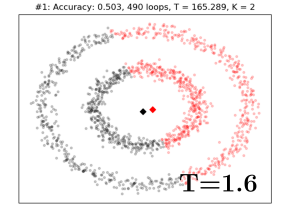
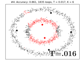
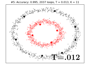
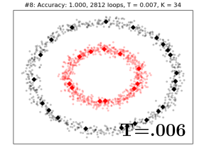
(a) Concentric circles.

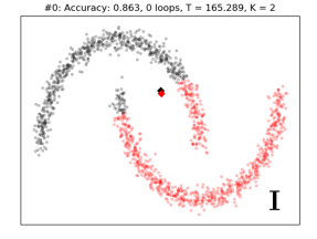
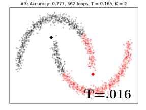
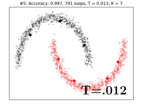
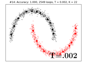
(b) Half moons.

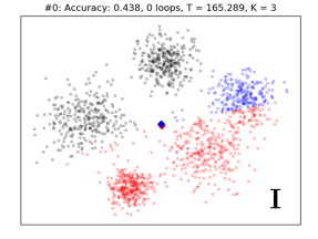
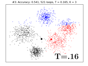
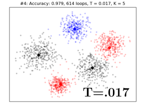
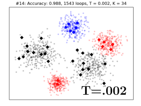
(c) Gaussians.

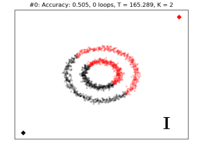
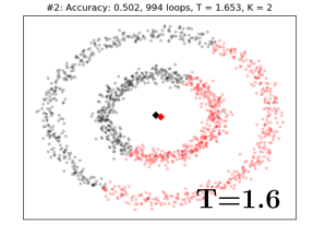
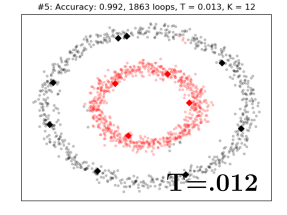
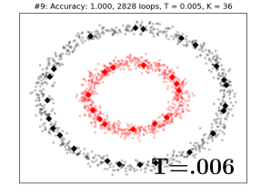
(d) Poor initial conditions.

Figure 1: $(a)$-$(c)$Illustration of the evolution of Alg. 1 for decreasing temperature $T$ in binary classification in 2D. $(d)$ Showcasing robustness with respect to bad initial conditions.

IV-A Toy Examples

We first showcase how Alg. 1 works in three simple, but illustrative, classification problems in two dimensions (Fig. 1). The first two are binary classification problems with the underlying class distributions shaped as concentric circles (Fig. 1(a)), and half moons (Fig. 1(b)), respectively. The third is a multi-class classification problem with Gaussian mixture class distributions (Fig. 1(c)). All datasets consist of $1500$ samples. Since the objective is to give a geometric illustration of how the algorithm works in the two-dimensional plane, the Euclidean distance is used. The algorithm starts at high temperature with a single codevector for each class. As the temperature coefficient gradually decreases (Fig. 1, from left to right), the number of codevectors progressively increases. The accuracy of the algorithm typically increases as well. As the temperature goes to zero, the complexity of the model, i.e. the number of codevectors, rapidly increases (Fig. 1, rightmost pictures). This may, or may not, translate to a corresponding performance boost. A single parameter –the temperature $T$– offers online control on this complexity-accuracy trade-off. Finally, Fig. 1(d) showcases the robustness of the proposed algorithm with respect to the initial configuration. Here the codevectors are poorly initialized outside the support of the data, which is not assumed known a priori (e.g. online observations of unknown domain). In this example the LVQ algorithm has been shown to fail [35]. In contrast, the entropy term $H$ in the optimization objective of Alg. 1, allows for the online adaptation to the domain of the dataset and helps to prevent poor local minima.

IV-B Real Datasets

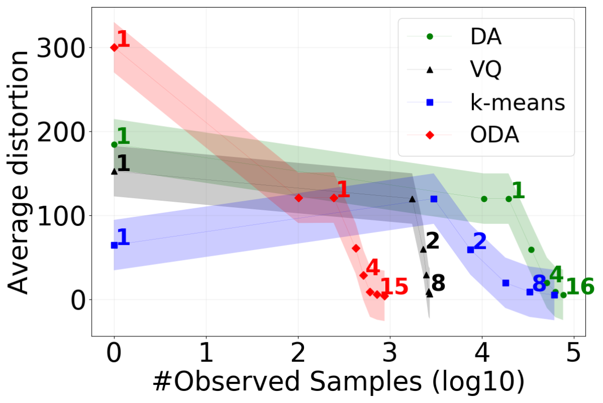
(a) Gaussians.

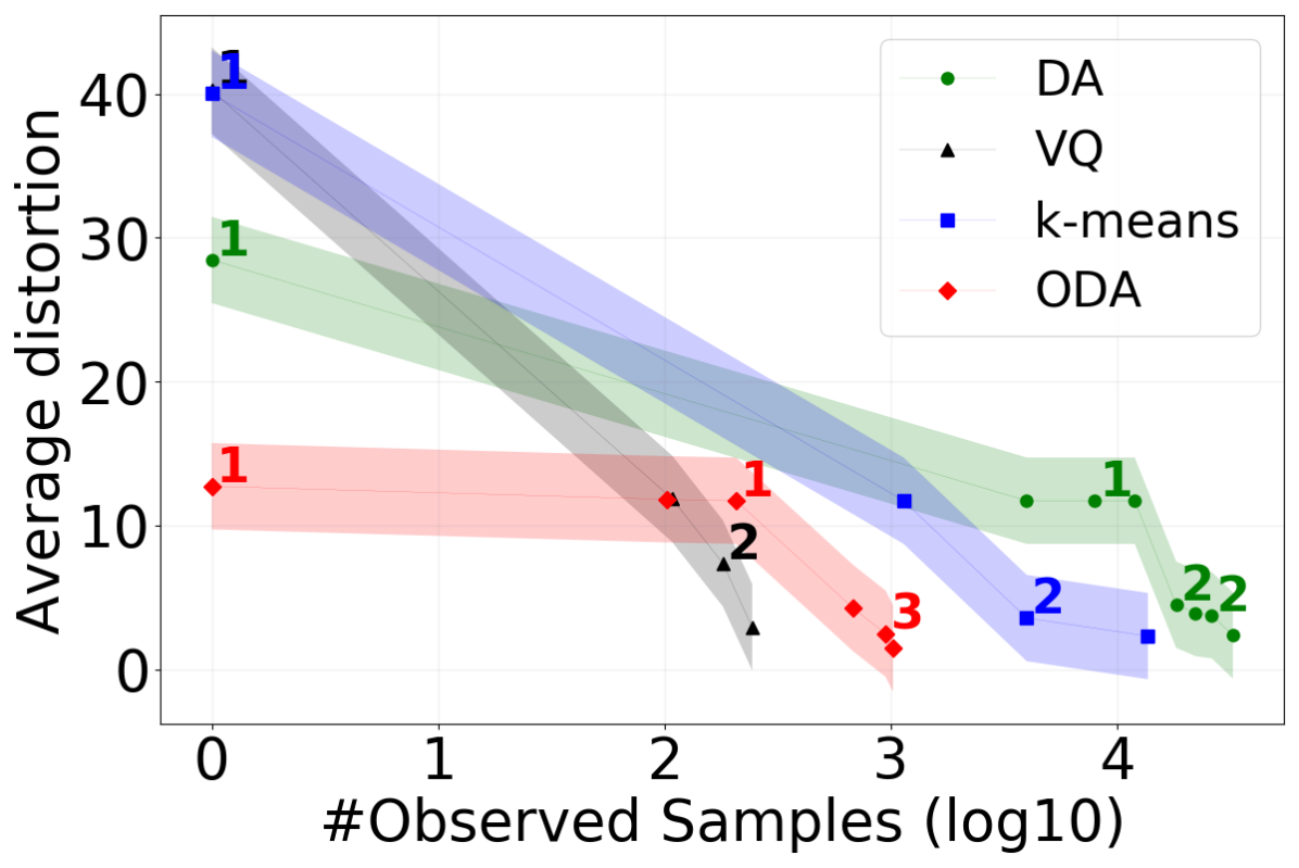
(b) WBCD.

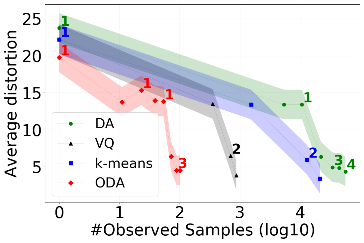
(c) PIMA.

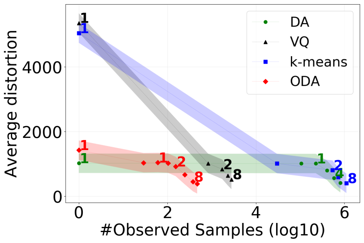
(d) Adult.

Figure 2: Algorithm comparison for clustering.

Clustering. For clustering, we consider the following datasets: (a) the dataset of Fig. 1(c) (Gaussians), (b) the WBCD dataset [36], (c) the PIMA dataset [37], and (d) the Adult dataset[36]. In Fig. 2, we compare Alg. 1 with the online sVQ algorithm (Def. 1), and two offline algorithms, namely $k$-means [27], and the original deterministic annealing (DA) algorithm [17]. The algorithms are compared in terms of the minimum average distortion achieved, as a function of the number of samples they observed, and the number of clusters they used (floating numbers inside the figures). The Euclidean distance is used for fair comparison. Since there is no criterion to decide the number of clusters $K$ for $k$-means and sVQ, we run them sequentially for the $K$ values estimated by DA, and add up the computational time. All algorithms are able to achieve comparable average distortion values given good initial conditions and appropriate size $K$. Therefore, the progressive estimation of $K$, as well as the robustness with respect to the initial conditions, are key features of both annealing algorithms, i.e., DA and ODA (Alg. 1). Compared to the offline algorithms, i.e., $k$-means and DA, ODA and sVQ achieve practical convergence with significantly smaller number of observations, which corresponds to reduced computational time, as argued above. Notice the substantial difference in running time between the original DA algorithm and the proposed ODA algorithm in Fig. 4. Compared to the online sVQ (and LVQ), the probabilistic approach of ODA introduces additional computational cost: all neurons are now updated in every iteration, instead of only the winner neuron. However, the updates can still be computed fast when using Bregman divergences (Theorem 2), and the aforementioned benefits of the annealing nature of ODA, outweigh this additional cost in many real-life problems.

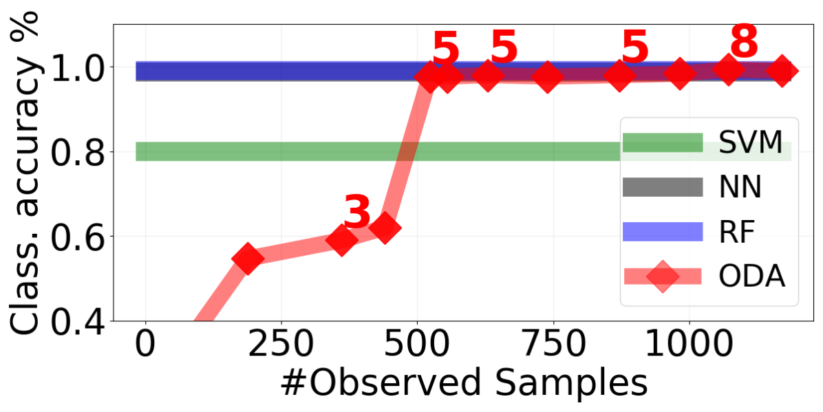
(a) Gaussians.

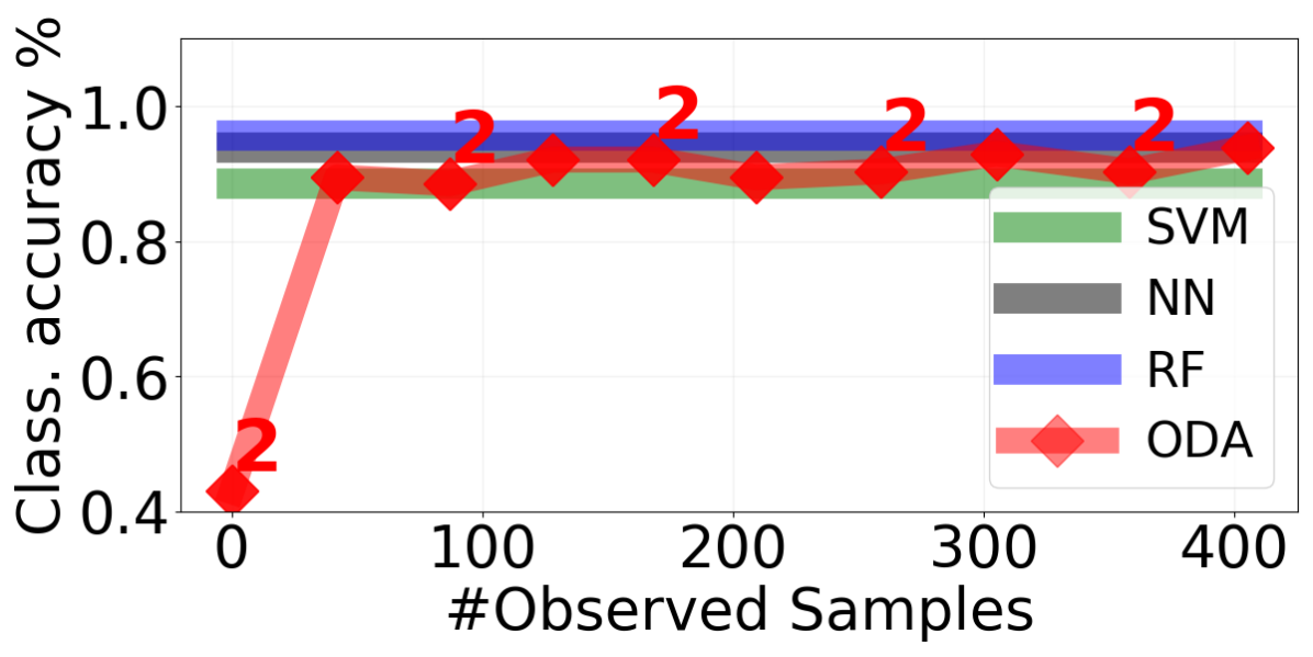
(b) WBCD.

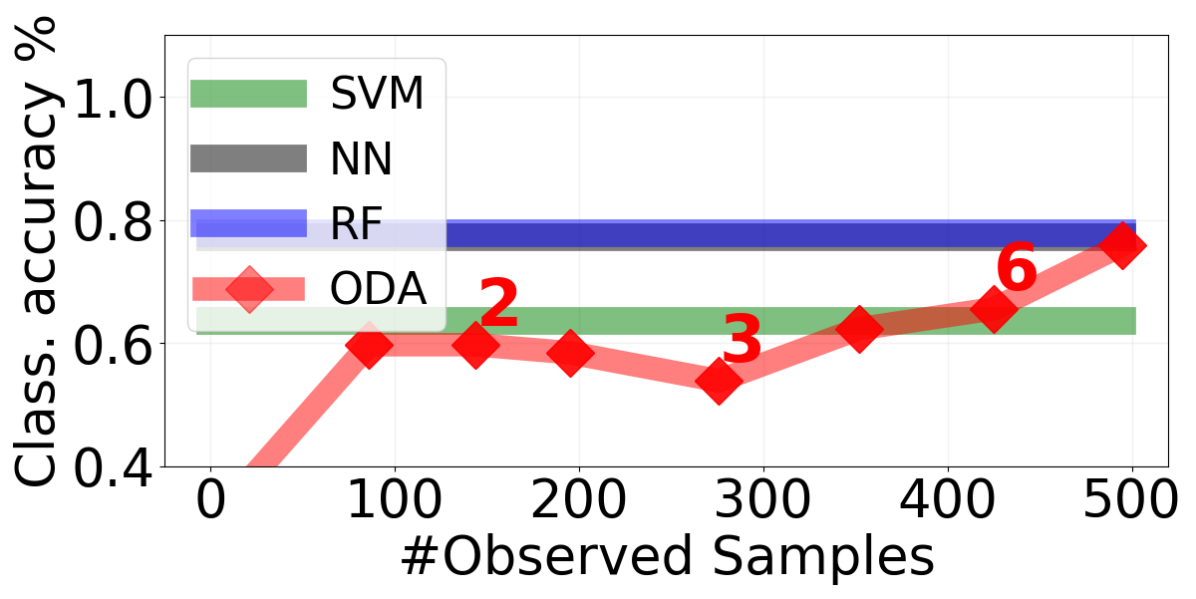
(c) PIMA.

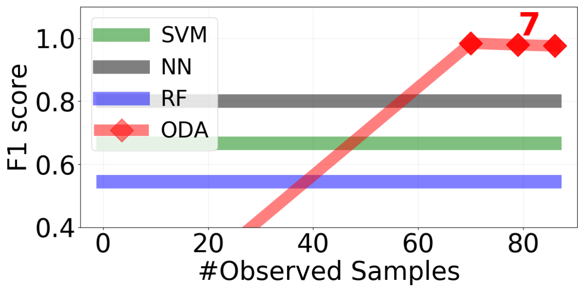
(d) Credit Card (F1 score).

Figure 3: Algorithm comparison for classification.

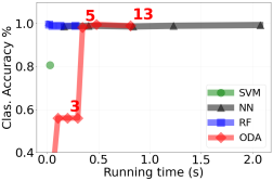
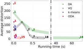
Figure 4: Running time of the algorithms in Fig. 2(a), Fig. 3(a).

Data set	ODA	SVM	NN	RF
Gaussian	98.9$\pm$ 0.0	79.5$\pm$ 0.0	98.6$\pm$ 0.0	98.7$\pm$ 0.0
WBCD	90.7$\pm$ 0.0	85.6$\pm$ 0.0	92.7$\pm$ 0.0	94.6$\pm$ 0.0
Credit (F1)	95.6$\pm$ 0.0	69.1$\pm$ 0.2	58.9$\pm$ 0.1	62.8$\pm$ 0.1
PIMA	70.5$\pm$ 0.0	62.9$\pm$ 0.0	76.3$\pm$ 0.0	74.4$\pm$ 0.0

TABLE I: Classification accuracies in $5$-fold cross-validation.

Classification. For classification, we consider the Gaussian (Fig. 1(c)), WBCD, PIMA, and Credit Card[38] datasets. We compare Alg. 1 against an SVM model with a linear kernel [39], a feed-forward fully-connected neural network with a single hidden layer of $n_{NN}$ neurons (NN), and the Random Forests (RF) algorithm with $t_{RF}$ estimators [40]. These algorithms have been selected to represent today’s standards in simple classification tasks, i.e., when no sophisticated feature extraction is required. The SVM classifier represents the class of linear classification models, the neural network represents the class of non-linear approximation models, and the random forests algorithm represents the class of partition-based methods with bootstrap aggregating. Table I shows the results of a $5$-fold cross validation ($80/20\%$), and Fig. 3 illustrates the performance of the algorithms during a random test. The evolution of the complexity of the ODA model is depicted as a function of the observed samples and the classification accuracy achieved. We use the generalized I divergence (Example 2) in the WBCD dataset and the Euclidean distance in the rest. ODA (Alg. 1) outperforms the linear SVM classifier, and can achieve comparable performance with the NN and the RF algorithms, which are today’s standards in classification tasks where no feature extraction is required. In the greatly unbalanced Credit Card dataset, all algorithms achieved accuracy close to $100\%$, but the $F1$ scores dropped significantly (Fig. 3(d)). Notably, this was not the case with the ODA algorithm. This may be due to the generative nature of the algorithm, and might also be an instance of the robustness expected by vector quantization algorithms [16]. Justifying and quantifying this robustness is beyond the scope of this paper.

Parameters. The parameters $n_{NN}\in[10,100]$ and $t_{RF}\in[10,100]$ were selected through extensive grid search. In contrast, the parameters of the ODA algorithm for all the experiments were set as follows: $T_{max}=100\Delta_{S}d$, $T_{min}=0.001\Delta_{S}d$, $K_{max}=100$, $\gamma=0.8$, $\epsilon_{c}=0.0001\Delta_{S}d$, $\epsilon_{n}=0.001\Delta_{S}d$, $\epsilon_{r}=10^{-7}$, $\delta=0.01\Delta_{S}d$, and $\alpha_{n}=\nicefrac{{1}}{{1+0.9n}}$, where $d$ is the number of dimensions of the input $X\in S\subseteq\mathbb{R}^{d}$, and $\Delta_{S}$ represents the length of the largest edge of the smallest $d$-orthotope that contains $S$. We stress that no parameter tuning has taken place for the proposed algorithm.

Limitations. Finally, we note that both NN and RF outperform Alg. 1 in some datasets (Table I). A fine-tuning mechanism, as discussed in Section III-E, could alleviate these differences, and is currently not used in our experiments. Regarding the running time of the ODA algorithm, Fig. 4 shows the execution time of the learning algorithms used in Fig. 2(a) and Fig. 3(a). All experiments were implemented in a personal computer. We note that, in contrast to the commercial, and, therefore, optimized versions of the $k$-means, SVM, NN, and RF algorithms, the algorithmic implementation of the proposed algorithm is not yet optimized, and substantial speed-up is expected through appropriate software development.

V Conclusion

It is understood that the trade-off between model complexity and performance in machine learning algorithms is closely related to over-fitting, generalization, and robustness to input perturbations and adversarial attacks. We investigate the properties of learning with progressively growing models, and propose an online annealing optimization approach as a learning algorithm that progressively adjusts its complexity with respect to new observations, offering online control over the performance-complexity trade-off. The proposed algorithm can be viewed as a neural network with inherent regularization mechanisms, the learning rule of which is formulated as an online gradient-free stochastic approximation algorithm. As a prototype-based learning algorithm, it offers a progressively growing knowledge base that can be interpreted as a memory unit that parallels similar concepts form cognitive psychology and neuroscience. The annealing nature of the algorithm prevents poor local minima, offers robustness to initial conditions, and provides a means to progressively increase the complexity of the learning model as needed. To our knowledge, this is the first time such a progressive approach has been proposed for machine learning applications. We believe that these results can lead to new developments in learning with progressively growing models, especially in communication, control, and reinforcement learning applications.

Christos N. Mavridis (M’20) received the Diploma degree in electrical and computer engineering from the National Technical University of Athens, Greece, in 2017, and the M.S. and Ph.D. degrees in electrical and computer engineering at the University of Maryland, College Park, MD, USA, in 2021. His research interests include learning theory, stochastic optimization, systems and control theory, multi-agent systems, and robotics. He has worked as a researcher at the Department of Electrical and Computer Engineering at the University of Maryland, College Park, and as a research intern for the Math and Algorithms Research Group at Nokia Bell Labs, NJ, USA, and the System Sciences Lab at Xerox Palo Alto Research Center (PARC), CA, USA. Dr. Mavridis is an IEEE member, and a member of the Institute for Systems Research (ISR) and the Autonomy, Robotics and Cognition (ARC) Lab. He received the Ann G. Wylie Dissertation Fellowship in 2021, and the A. James Clark School of Engineering Distinguished Graduate Fellowship, Outstanding Graduate Research Assistant Award, and Future Faculty Fellowship, in 2017, 2020, and 2021, respectively. He has been a finalist in the Qualcomm Innovation Fellowship US, San Diego, CA, 2018, and he has received the Best Student Paper Award (1st place) in the IEEE International Conference on Intelligent Transportation Systems (ITSC), 2021.

John S. Baras (LF’13) received the Diploma degree in electrical and mechanical engineering from the National Technical University of Athens, Greece, in 1970, and the M.S. and Ph.D. degrees in applied mathematics from Harvard University, Cambridge, MA, USA, in 1971 and 1973, respectively. He is a Distinguished University Professor and holds the Lockheed Martin Chair in Systems Engineering, with the Department of Electrical and Computer Engineering and the Institute for Systems Research (ISR), at the University of Maryland College Park. From 1985 to 1991, he was the Founding Director of the ISR. Since 1992, he has been the Director of the Maryland Center for Hybrid Networks (HYNET), which he co-founded. His research interests include systems and control, optimization, communication networks, applied mathematics, machine learning, artificial intelligence, signal processing, robotics, computing systems, security, trust, systems biology, healthcare systems, model-based systems engineering. Dr. Baras is a Fellow of IEEE (Life), SIAM, AAAS, NAI, IFAC, AMS, AIAA, Member of the National Academy of Inventors and a Foreign Member of the Royal Swedish Academy of Engineering Sciences. Major honors include the 1980 George Axelby Award from the IEEE Control Systems Society, the 2006 Leonard Abraham Prize from the IEEE Communications Society, the 2017 IEEE Simon Ramo Medal, the 2017 AACC Richard E. Bellman Control Heritage Award, the 2018 AIAA Aerospace Communications Award. In 2016 he was inducted in the A. J. Clark School of Engineering Innovation Hall of Fame. In 2018 he was awarded a Doctorate Honoris Causa by his alma mater the National Technical University of Athens, Greece.

References

- [1] K. P. Bennett and E. Parrado-Hernández, “The interplay of optimization and machine learning research,” The Journal of Machine Learning Research, vol. 7, pp. 1265–1281, 2006.
- [2] A. Krizhevsky, I. Sutskever, and G. E. Hinton, “Imagenet classification with deep convolutional neural networks,” in Advances in Neural Information Processing Systems, 2012, pp. 1097–1105.
- [3] H. Lee, R. Grosse, R. Ranganath, and A. Y. Ng, “Convolutional deep belief networks for scalable unsupervised learning of hierarchical representations,” in Proceedings of the 26th Annual International Conference on Machine Learning, 2009, pp. 609–616.
- [4] N. C. Thompson, K. Greenewald, K. Lee, and G. F. Manso, “The computational limits of deep learning,” arXiv:2007.05558, 2020.
- [5] E. Strubell, A. Ganesh, and A. McCallum, “Energy and policy considerations for deep learning in nlp,” arXiv:1906.02243, 2019.
- [6] C. Szegedy, W. Zaremba, I. Sutskever, J. Bruna, D. Erhan, I. Goodfellow, and R. Fergus, “Intriguing properties of neural networks,” arXiv preprint arXiv:1312.6199, 2013.
- [7] N. Carlini and D. Wagner, “Towards evaluating the robustness of neural networks,” in IEEE Symposium on Security and Privacy. IEEE, 2017.
- [8] V. Sehwag, A. N. Bhagoji, L. Song, C. Sitawarin, D. Cullina, M. Chiang, and P. Mittal, “Analyzing the robustness of open-world machine learning,” in Proceedings of the 12th ACM Workshop on Artificial Intelligence and Security, 2019, pp. 105–116.
- [9] H. Xu and S. Mannor, “Robustness and generalization,” Machine Learning, vol. 86, no. 3, pp. 391–423, 2012.
- [10] C. G. Northcutt, A. Athalye, and J. Mueller, “Pervasive label errors in test sets destabilize machine learning benchmarks,” arXiv preprint arXiv:2103.14749, 2021.
- [11] A. Raghunathan, S. M. Xie, F. Yang, J. C. Duchi, and P. Liang, “Adversarial training can hurt generalization,” arXiv:1906.06032, 2019.
- [12] T. Kohonen, Learning Vector Quantization. Berlin, Heidelberg: Springer Berlin Heidelberg, 1995, pp. 175–189.
- [13] L. Devroye, L. Györfi, and G. Lugosi, A probabilistic theory of pattern recognition. Springer Science & Business Media, 2013, vol. 31.
- [14] C. N. Mavridis and J. S. Baras, “Convergence of stochastic vector quantization and learning vector quantization with bregman divergences,” in 21rst IFAC World Congress. IFAC, 2020.
- [15] E. A. Uriarte and F. D. Martín, “Topology preservation in som,” International Journal of Applied Mathematics and Computer Sciences, vol. 1, no. 1, pp. 19–22, 2005.
- [16] S. Saralajew, L. Holdijk, M. Rees, and T. Villmann, “Robustness of generalized learning vector quantization models against adversarial attacks,” in International Workshop on Self-Organizing Maps. Springer, 2019, pp. 189–199.
- [17] K. Rose, “Deterministic annealing for clustering, compression, classification, regression, and related optimization problems,” Proceedings of the IEEE, vol. 86, no. 11, pp. 2210–2239, 1998.
- [18] V. S. Borkar, Stochastic approximation: a dynamical systems viewpoint. Springer, 2009, vol. 48.
- [19] A. Banerjee, S. Merugu, I. S. Dhillon, and J. Ghosh, “Clustering with bregman divergences,” Journal of Machine Learning Research, vol. 6, no. Oct, pp. 1705–1749, 2005.
- [20] T. Villmann, S. Haase, F.-M. Schleif, B. Hammer, and M. Biehl, “The mathematics of divergence based online learning in vector quantization,” in IAPR Workshop on Artificial Neural Networks in Pattern Recognition. Springer, 2010, pp. 108–119.
- [21] C. N. Mavridis and J. S. Baras, “Progressive graph partitioning based on information diffusion,” in Conference on Decision and Control (CDC). IEEE, 2021, pp. 37–42.
- [22] C. N. Mavridis, N. Suriyarachchi, and J. S. Baras, “Detection of dynamically changing leaders incomplex swarms from observed dynamic data,” in 2020 Conference on Decision and Game Theory for Security (GameSec), 2020.
- [23] ——, “Maximum-entropy progressive state aggregation for reinforcement learning,” in Conference on Decision and Control (CDC). IEEE, 2021, pp. 5144–5149.
- [24] M. Biehl, B. Hammer, and T. Villmann, “Prototype-based models in machine learning,” Wiley Interdisciplinary Reviews: Cognitive Science, vol. 7, no. 2, pp. 92–111, 2016.
- [25] Y. Linde, A. Buzo, and R. Gray, “An algorithm for vector quantizer design,” IEEE Transactions on Communications, vol. 28, 1980.
- [26] M. Sabin and R. Gray, “Global convergence and empirical consistency of the generalized lloyd algorithm,” IEEE Transactions on Information Theory, vol. 32, no. 2, pp. 148–155, 1986.
- [27] L. Bottou and Y. Bengio, “Convergence properties of the k-means algorithms,” in Advances in Neural Information Processing Systems, 1995, pp. 585–592.
- [28] R. O. Duda, P. E. Hart, and D. G. Stork, Pattern classification. John Wiley & Sons, 2012.
- [29] A. Sato and K. Yamada, “Generalized learning vector quantization,” in Advances in Neural Information Processing Systems, 1996, pp. 423–429.
- [30] B. Hammer and T. Villmann, “Generalized relevance learning vector quantization,” Neural Networks, vol. 15, no. 8-9, pp. 1059–1068, 2002.
- [31] H. K. B. Babiker and R. Goebel, “Using kl-divergence to focus deep visual explanation,” arXiv preprint arXiv:1711.06431, 2017.
- [32] E. T. Jaynes, “Information theory and statistical mechanics,” Physical Review, vol. 106, no. 4, p. 620, 1957.
- [33] K. Miettinen, Nonlinear multiobjective optimization. Springer Science & Business Media, 2012, vol. 12.
- [34] H. Robbins and S. Monro, “A stochastic approximation method,” The Annals of Mathematical Statistics, pp. 400–407, 1951.
- [35] J. S. Baras and A. LaVigna, “Convergence of a neural network classifier,” in Advances in Neural Information Processing Systems, 1991.
- [36] D. Dua and C. Graff, “UCI machine learning repository,” 2017. [Online]. Available: http://archive.ics.uci.edu/ml
- [37] J. W. Smith, J. Everhart, W. Dickson, W. Knowler, and R. Johannes, “Using the adap learning algorithm to forecast the onset of diabetes mellitus,” in Proceedings of the Annual Symposium on Computer Application in Medical Care. American Medical Informatics Association, 1988, p. 261.
- [38] F. Carcillo, Y.-A. Le Borgne, O. Caelen, Y. Kessaci, F. Oblé, and G. Bontempi, “Combining unsupervised and supervised learning in credit card fraud detection,” Information Sciences, 2019.
- [39] M. A. Hearst, S. T. Dumais, E. Osuna, J. Platt, and B. Scholkopf, “Support vector machines,” IEEE Intelligent Systems and their Applications, vol. 13, no. 4, pp. 18–28, 1998.
- [40] L. Breiman, “Random forests,” Machine Learning, vol. 45, 2001.