On the Performance of the Primary and Secondary Links in a 3-D Underlay Cognitive Molecular Communication

Abstract

Molecular communication often involves coexisting links where certain links may have priority over others. In this work, we consider a system in three-dimensional (3-D) space with two coexisting communication links, each between a point transmitter and fully-absorbing spherical receiver (FAR), where the one link (termed primary) has priority over the second link (termed secondary). The system implements the underlay cognitive-communication strategy for the co-existence of both links, which use the same type of molecules for information transfer. Mutual influence of FARs existing in the same communication medium results in competition for capturing the information-carrying molecules. In this work, first, we derive an approximate hitting probability equation for a diffusion-limited molecular communication system with two spherical FARs of different sizes considering the effect of molecular degradation. The derived equation is then used for the performance analysis of primary and secondary links in a cognitive molecular communication scenario. We show that the simple transmit control strategy at the secondary transmitter can improve the performance of the overall system. We study the influence of molecular degradation and decision threshold on the system performance. We also show that the systems parameters need to be carefully set to improve the performance of the system.

I Introduction

Molecular communication (MC) is the communication between the transmitter and the receiver by using information molecules (IMs) as the carrier of information [1, 2]. Among different propagation mechanisms, molecular communication via diffusion (MCvD) systems is the most popular, mainly due to the ease of mathematical modeling and its energy efficiency. In MCvD systems, bio-nanomachines (nanomachines with biological components) can be used as the transmitter and receiver. Since the capabilities of individual bio-nanomachines may be limited to simple sensing and actuation, the internet of bio-nano things (IoBNT) [3] is envisioned to enable the interconnection of several bio-nanomachines to perform complex tasks. Applications of IoBNT include intra-body sensing and actuation, connectivity control, control of toxic gases and pollution in the environment [3], and diagnosis and mitigation of infectious diseases [4].

Related works: In an MCvD system with multiple communication links, some communication links may have priority over others. For example, inside the human body, an artificial MC link would have to co-exist with existing biological links that are inherent in the body, and these biological links have priority over the artificial link. Interference beyond a threshold from the MC link on any biological link may disrupt the human-body activities when both links use the same type of IMs. Similarly, a bio-nanomachine sensing the blood sugar level inside a diabetic person can have priority over the bio-nanomachine sensing the body temperature. In systems with multiple coexisting links with different priorities, the one with higher priority is termed primary link and the rest are termed secondary links. The goal here is to allow secondary link communication while ensuring a certain quality of serviec (QoS) at the primary. In wireless communication, these systems are called cognitive radio, where information like channel conditions, messages, codebooks, etc., are utilized for the co-existence of the links[5, 6]. The three different strategies used in cognitive radio are underlay, overlay, and interweave. In the underlay strategy, the secondary transmitter controls the transmit power to limit the co-channel interference at primary receiver [6]. In the overlay strategy, the secondary transmitter assists the primary communication via relaying or interference cancellation with the help of transmit and channel information provided by the primary. In the interleaving strategy, the secondary transmitter transmits its information only when it does not sense any primary communication.

Analogous paradigms have been recently proposed for molecular communication[7, 8, 9, 10, 11]. Authors in [7] studied an interweaving MC system where the secondary transmitter intelligently senses the absence of primary transmission in the primary transmitter communication. A framework for a system with co-existing MC and the biochemical system was discussed in [8] where some enzymes are introduced to reduce the inter-symbol interference (ISI) to the MC system, and the perturbation of the biochemical system was analyzed along with the equilibrium of the biochemical system. [9] studied an underlay cognitive-communication consisting of biological systems and an MC link. However the work is limited to the time evolution of the concentration of molecules and scaling laws for the probability of a molecule to reach the receiver. The study in [10] utilise Kullback-Leibler divergence between the distribution of molecules on the surface of biological system in the presence and absence of MC system for the coexistence constraint. The work in [9, 10] are initial models developed based on the theory of chemical reaction networks and many modeling complexities including receiver size, geometry, and the mutual influence between receivers are not considered. In [11], a passive receiver is used as the receiver and coexistence constraint is obtained with the help of reactive signaling.

Unlike wireless communication, in MC with absorbing receivers, the links face interference from transmitters as well as receivers that are present in the same media. This is due to the fact that such receivers will cause IMs corresponding to a communication link to get absorbed at itself, which will reduce the number of IMs reaching the desired receiver. Since multiple receivers coexist in cognitive systems, it is essential to characterize the impact of receivers on each other in order to evaluate the performance of these systems. Many previous works including [7, 8, 9, 10] ignore the mutual influence of absorbing receivers due to lack of its analytic expressions in the literature. An approximate analytical expression for the hitting probability of an IM on any of the FAR (centers distributed as Poisson point process) is given in [12]. For an MCvD system with two FARs of equal size, an approximate equation for the hitting probability of an IM on each of the FAR was derived in our previous work [13]. However, in cognitive systems, primary and secondary receivers can be of different sizes whose expressions are unknown in the past literature. Therefore, it is essential to consider the difference in the size of receivers in the system model.

In this paper, we try to bridge these gaps by first characterizing the hitting probability of IMs on each FAR and then provide an analytical framework to study an underlay cognitive MC system using the derived expressions.

Contributions: In this work, we develop an analytical framework to study a cognitive molecular communication system with a primary link and a secondary link implementing transmit control to limit interference at the primary link (i.e., underlay). For the same, we first characterize the mutual impact of receivers on each other by deriving an approximate closed expression for the hitting probability of an IM on each of the FARs in the presence of the other FAR when they have different radii. In this paper, we also consider that the IMs in the propagation medium can undergo molecular degradation [14] in deriving the hitting probability of an IM on each of the FARs. We then apply the derived results in the proposed analytical framework to study the performance of the considered underlay cognitive molecular communication in which the secondary transmission is controlled to limit the co-channel interference at the primary receiver below a certain level. The main contributions of this work are listed below.

1. We derive an approximate closed form expression for the hitting probability of an information molecule hitting each of the fully-absorbing receivers of different radii in a two-receiver system, which is an extension of the work done in [13].

2. We derive an approximate equation for the hitting probability of a degradable information molecule hitting each of the fully-absorbing receivers of different radii in a two-receiver system.

3. Based on the derived hitting probability expressions, we develop several important insights.

4. We model a 3-D diffusion-limited cognitive molecular communication system with primary and secondary transmitter-receiver pairs. We consider an underlay strategy where the number of transmit molecules at the secondary transmitter is controlled to limit the co-channel interference at the primary receiver under a certain threshold.

5. We derive the performance of the primary and the secondary links in terms of expected interference and bit error probability of both links. Several key insights are developed regarding optimal system parameters, gains due to transmit control strategy, and feasibility of cognition.

The important symbols and notation used in this work is given in Table I.

TABLE I: Notation Summary

Symbol	Definition
$D$	Diffusion coefficient of the IMs in the propagation medium.
$\mu$	Degradation rate constant of the IM.
$T_{\mathrm{b}}$	Bit duration.
$\square_{\mathrm{P}},\ \square_{\mathrm{S}}$	Parameters related to the primary and secondary links respectively.
$\boldsymbol{x}_{i},\ \boldsymbol{y}_{i}$	Locations of TXi and FARi in $\mathbb{R}^{3}$. $i\in\{\mathrm{P},\mathrm{S}\}$
$\bar{i}$	Denote compliment for $i\in\{\mathrm{P},\mathrm{S}\}$. i.e., $\bar{\mathrm{S}}=\mathrm{P}$ and $\bar{\mathrm{P}}=\mathrm{S}$.
$r_{{}_{\mathrm{SP}}}$	Distance between TXS and the center of FARP.
$q_{bm}$	Probability of sending the bit $\mathsf{b}\in\{0,1\}$ by the TXm.
$b_{i}[k]$	Information bit transmitted by the TXi in the $k$th time-slot.
$u_{{{}_{\mathrm{P}}}}[k],\newline u_{{{}_{\mathrm{S}}}}[r_{{}_{\mathrm{SP}}};k]$	Number of molecules emitted by primary and secondary transmitter in the $k$th time-slot.
$\mathrm{p}_{mi}\left({t,\mu}\right)$	Probability of an IM of degradation rate constant $\mu$ emitted by the TXm hitting on FARi within time $t$ in the presence of the other FAR.
$\mathrm{p}_{mi}\left({t}\right)$	Probability of an IM emitted by the TXm hitting on FARi within time $t$ in the presence of the other FAR. Here $\mu=0s^{-1}$.
$h_{mi}[l-k]$	Probability that a IM transmitted by TXm in the slot $k\in\{1,2,\cdots,l\}$ arrives at FARi in time-slot $l$.
$z_{mi}[l;k]$	Number of molecules received at the FARi in $l$th slot due to the emission of molecules from the TXm at the $k$th slot.
$z_{i}[l]$	The total number of IMs observed at the FARi in the $l$th time-slot.
$\eta[i;l]$	Detection threshold at the FARi in the $l$th time-slot.
$\mathrm{P}_{\mathrm{e}i,0}[l],\ \mathrm{P}_{\mathrm{e}i,1}[l]$	The probabilities of incorrect decoding for bit 0 and 1, respectively at the $l$th time-slot.
$\mathrm{P}_{\mathrm{e}i}[l]$	Total probability of error at the $l$th time-slot.

II System Model

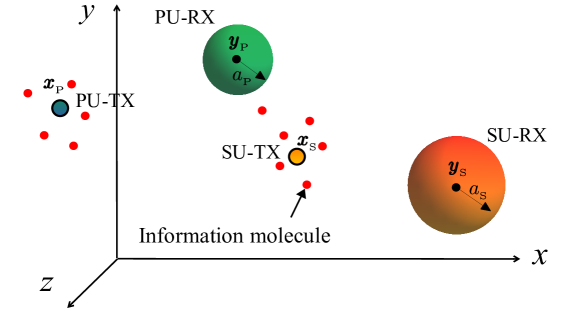
Figure 1: Schematic diagram of a 3-D diffusive cognitive molecular communication system where a secondary point transmitter is communicating with a secondary spherical FAR in presence of ongoing communication between primary point transmitter and spherical FAR.

This work considers a 3-D diffusion-limited scenario, with primary and secondary (cognitive) transmitter-receiver pairs, as shown in Fig. 1. The primary and secondary links coexist in the communication medium with higher performance priority given to the primary link. The primary transmitter-receiver pair is unaware of the secondary transmission. In contrast, the secondary transmitter intelligently controls the number of transmit molecules so that the interference caused by the secondary transmitter on the primary receiver is below a threshold value in all time-slots. This strategy of communication is called underlay cognitive-communication.

II-A Network Model

The location of each of the communicating nodes is assumed to be fixed in the 3-D medium. Each transmitter is a point source, which can emit molecules into the propagation medium. Each receiver is assumed to be spherical FAR, which absorbs all the molecules hitting its surface and counts them for decoding purpose. Let the primary point transmitter (TX_P), primary FAR (FAR_P), secondary point transmitter (TX_S) and secondary FAR (FAR_S) be located at positions $\boldsymbol{x}_{{{}_{\mathrm{P}}}},\ \boldsymbol{y}_{{}_{\mathrm{P}}},\ \boldsymbol{x}_{{}_{\mathrm{S}}}$ and $\boldsymbol{y}_{{}_{\mathrm{S}}}$ respectively, in the $\mathbb{R}^{3}$ space. The FAR_P and FAR_S are spherical fully-absorbing receivers of radius $a_{{}_{\mathrm{P}}}$ and $a_{{}_{\mathrm{S}}}$, respectively. Both primary and secondary transmitter-receiver pairs use the same type of molecules as the carrier of information. Similar to several existing work such as [15], the transmitters and the receivers are assumed to be synchronized in time.

II-B Modulation and Transmission Model

Consider that the transmitters emit molecules at the beginning of a time-slot of duration $T_{\mathrm{b}}$. Let $b_{{}_{\mathrm{P}}}[l]$ and $b_{{}_{\mathrm{S}}}[l]$ denote the information bit transmitted by the TX_P and TX_S respectively, at the $l$th time-slot. The bit $b_{m}[l],m\in\{\mathrm{P},\mathrm{S}\}$ can be considered to be Bernoulli distributed with parameter $q_{1m}$. We consider on-off keying (OOK) modulation for both transmissions. For primary communication, at the beginning of the time-slot, the TX_P emits a fixed number ($u_{{{}_{\mathrm{P}}}}[l]=N$) of molecules for a bit $1$ and does not emit molecules for a bit $0$. However, for secondary-communication, the TX_S emits a variable $u_{{{}_{\mathrm{S}}}}[r_{{}_{\mathrm{SP}}};l]$ number of molecules for bit 1 and 0 molecules for bit 0 in any slot $l$. For cognitive communication, the number of molecules $u_{{{}_{\mathrm{S}}}}[r_{{}_{\mathrm{SP}}};l]$ is controlled according to system parameters (in particular, $r_{{}_{\mathrm{SP}}}$ which is the distance between TX_S and the center of FAR_P. i.e., $\left\lVert\boldsymbol{y}_{{}_{\mathrm{P}}}-\boldsymbol{x}_{{}_{\mathrm{S}}}\right\rVert$) to minimize the TX_S interference at FAR_P. It can also vary with $l$ to have a better control on interference. The detailed derivation of $u_{{{}_{\mathrm{S}}}}[r_{{}_{\mathrm{SP}}};l]$ considering the maximum and proportional interfering molecules constraints is given in Section III.

II-C Propagation Model

We consider a pure diffusion-based propagation of IMs in this work. The IMs emitting from the TX_P and TX_S travel in the communication medium via 3-D Brownian motion [16]. Further these IMs degrade over time with a degradation rate constant $\mu$. Further, we consider that there are no potential collisions between the molecules when they propagate in the medium, and the molecules are immediately absorbed once they reach any one of the receivers. The diffusion coefficient for IMs is $D$ which is assumed to be constant everywhere in medium..

II-D Channel Model

Let $\mathrm{p}_{mi}\left({t,\mu}\right)$ denote the probability of an IM (with degradation rate constant $\mu$) emitted by the TX_m hitting on FAR_i within time $t$ in the presence of the another FAR FAR${}_{\bar{i}}$ ($m,i\in\{\mathrm{P},\mathrm{S}\}$). Let $h_{mi}[l-k]$ denote the probability that a IM transmitted by TX_m in slot $k\in\{1,2,\cdots,l\}$ arrives at FAR_i in time-slot $l$. Therefore,

$$h_{mi}[l-k]=\mathrm{p}_{mi}\left({(l-k+1)T_{\mathrm{b}},\mu}\right)-\mathrm{p}_{mi}\left({(l-k)T_{\mathrm{b}},\mu}\right).$$ (1)

II-E Receiver Observation

Let us focus on the current time slot denoted by $l$. Recall that, the transmit bit of the TX_m ($m\in\{\mathrm{P},\mathrm{S}\}$) at the $l$th time-slot (i.e., $b_{m}[l]$) is Bernoulli distributed.

II-E1 Observation at the FAR_P

Let us denote the number of received IMs at the FAR_P corresponding to the transmission of bit $b_{{}_{\mathrm{P}}}[l]\in\{0,1\}$ from the TX_P in the current time-slot as $z_{{}_{\mathrm{PP}}}[l;l]$. This quantity follows Binomial distribution with parameters $b_{{}_{\mathrm{P}}}[l]u_{{{}_{\mathrm{P}}}}[l]$ and $h_{{}_{\mathrm{PP}}}[0]$ i.e., $z_{{}_{\mathrm{PP}}}[l;l]\sim\mathcal{B}(b_{{}_{\mathrm{P}}}[l]u_{{{}_{\mathrm{P}}}}[l],h_{{}_{\mathrm{PP}}}[0])$. This is due to fact that each IM’s hit is a Bernoulli random variable with parameter $h_{{}_{\mathrm{PP}}}[0]$, and each IM’s propagation is independent of others.

Due to Brownian motion, IMs emitted in previous $l-1$ time-slots also hits the receiver in the current and upcoming time-slots, resulting in inter-symbol interference (ISI). The number of stray molecules observed at the FAR_P in the $l$th time-slot due to the emission from the previous $k$th time-slot is denoted by $z_{{}_{\mathrm{PP}}}[l;k],\ 1\leq k\leq l-1$. Similar to $z_{{}_{\mathrm{PP}}}[l;l]$, $z_{{}_{\mathrm{PP}}}[l;k]$ also follows Binomial distribution with parameters $b_{{}_{\mathrm{P}}}[k]u_{{{}_{\mathrm{P}}}}[k]$ and $h_{{}_{\mathrm{PP}}}[l-k]$, i.e., $z_{{}_{\mathrm{PP}}}[l;k]\sim\mathcal{B}\left(b_{{}_{\mathrm{P}}}[k]u_{{{}_{\mathrm{P}}}}[k],h_{{}_{\mathrm{PP}}}[l-k]\right)$. Therefore, the total number of ISI molecules observed at the FAR_P at the $l$th time-slot is $I_{{}_{\mathrm{PP}}}[l]=\sum_{k=1}^{l-1}z_{{}_{\mathrm{PP}}}[l;k]$.

Due to the presence of the secondary communication link, the IMs from the TX_S also reaches the FAR_P. Since both links are using same type of IMs, FAR_P cannot distinguish between them, resulting in co-channel interference (CCI) [17]. The number of interfering IMs reaching the FAR_P corresponding to the transmission of bit $b_{{}_{\mathrm{S}}}[k]$ by the TX_S in the $k$th time-slot is denoted by $z_{{}_{\mathrm{SP}}}[l;k],\ 1\leq k\leq l$. Note that, $z_{{}_{\mathrm{SP}}}[l;k]$ is Binomial distributed with parameters $b_{{}_{\mathrm{S}}}[k]u_{{{}_{\mathrm{S}}}}[r_{{}_{\mathrm{SP}}};k]$ and $h_{{}_{\mathrm{SP}}}[l-k]$ i.e., $z_{{}_{\mathrm{SP}}}[l;k]\sim\mathcal{B}\left(b_{{}_{\mathrm{S}}}[k]u_{{{}_{\mathrm{S}}}}[r_{{}_{\mathrm{SP}}};k],h_{{}_{\mathrm{SP}}}[l-k]\right)$. The total CCI molecules observed at the FAR_P is $C_{{}_{\mathrm{SP}}}[l]=\sum_{k=1}^{l}z_{{}_{\mathrm{SP}}}[l;k]$.

Therefore, the total number of IMs observed at the FAR_P in the $l$th time-slot is,

$$z_{{}_{\mathrm{P}}}[l]=z_{{}_{\mathrm{PP}}}[l;l]+\underbrace{\sum_{k=1}^{l-1}z_{{}_{\mathrm{PP}}}[l;k]}_{\triangleq I_{{}_{\mathrm{PP}}}[l]}+\underbrace{\sum_{k=1}^{l}z_{{}_{\mathrm{SP}}}[l;k]}_{\triangleq C_{{}_{\mathrm{SP}}}[l]}.$$ (2)

II-E2 Observation at the FAR_S

Similarly, the total number of IMs observed at the FAR_S is the sum of molecules observed at the receiver due to IMs emitted by the TX_S in the current slot and past $l-1$ slots (ISI molecules), and IMs emitted by the TX_P in the current and previous slots (CCI molecules).

The number of received IMs at the FAR_S corresponding to the transmission of bit $b_{{}_{\mathrm{S}}}[l]\in\{0,1\}$ in the current $l$th time-slot is $z_{{}_{\mathrm{SS}}}[l;l]$, where $z_{{}_{\mathrm{SS}}}[l;l]\sim\mathcal{B}(b_{{}_{\mathrm{S}}}[l]u_{{{}_{\mathrm{S}}}}[r_{{}_{\mathrm{SP}}};l],h_{{}_{\mathrm{SS}}}[0])$. The total number of ISI molecules observed at the FAR_S is $I_{{}_{\mathrm{SS}}}[l]=\sum_{k=1}^{l-1}z_{{}_{\mathrm{SS}}}[l;k]$, where $z_{{}_{\mathrm{SS}}}[l;k]\sim\mathcal{B}\left(b_{{}_{\mathrm{S}}}[k]u_{{{}_{\mathrm{S}}}}[r_{{}_{\mathrm{SP}}};k],h_{{}_{\mathrm{SS}}}[l-k]\right)$ and $b_{{}_{\mathrm{S}}}[k]$ is the bit transmitted by the TX_S in previous $k$th time-slot. The total number of CCI molecules absorbed at the FAR_S is $C_{{}_{\mathrm{PS}}}[l]=\sum_{k=1}^{l}z_{{}_{\mathrm{PS}}}[l;k]$, where $z_{{}_{\mathrm{PS}}}[l;k]\sim\mathcal{B}\left(b_{{}_{\mathrm{P}}}[k]u_{{{}_{\mathrm{P}}}}[k],h_{{}_{\mathrm{PS}}}[l-k]\right)$.

Therefore, the total number of IMs observed at the FAR_S in the $l$th time-slot is,

$$z_{{}_{\mathrm{S}}}[l]=z_{{}_{\mathrm{SS}}}[l;l]+\underbrace{\sum_{k=1}^{l-1}z_{{}_{\mathrm{SS}}}[l;k]}_{\triangleq I_{{}_{\mathrm{SS}}}[l]}+\underbrace{\sum_{k=1}^{l}z_{{}_{\mathrm{PS}}}[l;k]}_{\triangleq C_{{}_{\mathrm{PS}}}[l]}.$$ (3)

III Transmit Control at the Secondary Transmitter

We now describe the transmit control mechanism at TX_S to maintain certain QoS for the primary link. Since the priority is given to the primary link, the interference from the secondary link must not affect the performance of the primary link beyond a predefined limit. This is ensured by adapting the number of IMs emitted by TX_S (i.e., $u_{{{}_{\mathrm{S}}}}[r_{{}_{\mathrm{SP}}};l]$) according to the channel between the FAR_P and TX_S (which depends on $r_{{}_{\mathrm{SP}}}$ only). Further, since the total interference also depends on the previous transmission due to ISI, $u_{{{}_{\mathrm{S}}}}[r_{{}_{\mathrm{SP}}};l]$ may also need to be adjusted for each slot. Hence, $u_{{{}_{\mathrm{S}}}}[r_{{}_{\mathrm{SP}}};l]$ will be a function of $r_{{}_{\mathrm{SP}}}$ and the current slot index $l$. In this section, we derive the expression for the number of molecules allowed to be emitted by the TX_S in the $l$th time-slot so that the interference caused at the FAR_P is below a desired threshold value $u_{\mathrm{M}}$.

In other words, the transmitted number of molecules $u_{{{}_{\mathrm{S}}}}[r_{{}_{\mathrm{SP}}};l]$ by the TX_S is controlled such that the variation in $r_{{}_{\mathrm{SP}}}$ and $l$ does not result in the average number of interfering molecules cross beyond an acceptable threshold $u_{\mathrm{M}}$ i.e.,

$$\mathbb{E}\left[C_{{}_{\mathrm{SP}}}[l]\right]=\mathbb{E}\left[\sum_{k=1}^{l}z_{{}_{\mathrm{SP}}}[l;k]\right]\leq u_{\mathrm{M}}.$$ (4)

The term $\mathbb{E}\left[C_{{}_{\mathrm{SP}}}[l]\right]$ in (4) can be further solved as

$$\mathbb{E}\left[C_{{}_{\mathrm{SP}}}[l]\right]= \sum_{k=1}^{l}\mathbb{E}\left[z_{{}_{\mathrm{SP}}}[l;k]\right]$$

$$= \sum_{k=1}^{l}\mathbb{P}\left[b_{{}_{\mathrm{S}}}[k]=1\right]\mathbb{E}\left[z_{{}_{\mathrm{SP}}}[l;k]|b_{{}_{\mathrm{S}}}[k]=1\right]+\mathbb{P}\left[b_{{}_{\mathrm{S}}}[k]=0\right]\mathbb{E}\left[z_{{}_{\mathrm{SP}}}[l;k]|b_{{}_{\mathrm{S}}}[k]=0\right]$$

$$= q_{{}_{1\mathrm{S}}}\sum_{k=1}^{l}u_{{{}_{\mathrm{S}}}}[r_{{}_{\mathrm{SP}}};k]h_{{}_{\mathrm{SP}}}[l-k].$$ (5)

Further, due to the limited capacity of bio-nanomachines to generate a large number of molecules at a time, $u_{{{}_{\mathrm{S}}}}[r_{{}_{\mathrm{SP}}};l]$ is upper bounded by the maximum number of molecules available to transmit, $u_{\mathrm{L}}$. Now from (4) and (5), the number of IMs allowed to be transmitted by TX_S is given as

$$u_{{{}_{\mathrm{S}}}}[r_{{}_{\mathrm{SP}}};l]=\left\lfloor\min\left\{u_{\mathrm{L}},\frac{1}{h_{{}_{\mathrm{SP}}}[0]}\left(\frac{u_{\mathrm{M}}}{q_{{}_{1\mathrm{S}}}}-\sum_{k=1}^{l-1}u_{{{}_{\mathrm{S}}}}[r_{{}_{\mathrm{SP}}};k]h_{{}_{\mathrm{SP}}}[l-k]\right)^{+}\right\}\right\rfloor,$$ (6)

where $(x)^{+}=\max(x,0)$. The transmitted number of molecules by the TX_S is a function of $r_{{}_{\mathrm{SP}}}$. Therefore, the TX_S has to estimate the distance ($r_{{}_{\mathrm{SP}}}$) [18, 19] in a practical implementation [20]. Also, the TX_S has to store the values of $u_{{{}_{\mathrm{S}}}}[r_{{}_{\mathrm{SP}}};k],\ 1\leq k\leq l-1$ at any time-slot $l$. At large $l$ (i.e., steady state), $u_{{{}_{\mathrm{S}}}}[r_{{}_{\mathrm{SP}}};l]$ may become constant with time $l$.

Remark 1.

The lower bound on the number of transmitted molecules by the TX_S at any time-slot $l$ is zero. $u_{{{}_{\mathrm{S}}}}[r_{{}_{\mathrm{SP}}};l]$ equals to zero when $q_{{}_{1\mathrm{S}}}\sum_{k=1}^{l-1}u_{{{}_{\mathrm{S}}}}[r_{{}_{\mathrm{SP}}};k]h_{{}_{\mathrm{SP}}}[l-k]\geq u_{\mathrm{M}}$. That is, the number of transmitted molecules by the TX_S at any time-slot $l$ becomes zero when the average co-channel interference due to ISI is greater than the maximum allowed interference at the FAR_P (i.e., $u_{\mathrm{M}}$). In this scenario, the secondary communication ceases while primary communication remains unaffected.

Remark 2.

For a system without ISI, the number of molecules transmitted by the cognitive transmitter in any time slot is

$$u_{{{}_{\mathrm{S}}}}[r_{{}_{\mathrm{SP}}};l]=\left\lfloor\min\left\{u_{\mathrm{L}},\frac{u_{\mathrm{M}}}{q_{{}_{1\mathrm{S}}}h_{{}_{\mathrm{SP}}}[0]}\right\}\right\rfloor.$$ (7)

Systems with large time-slot duration and/or fast molecule degradation have negligible number of ISI molecules and hence (7) will be valid for them also.

Remark 3.

At the steady state (large $l$), the number of molecules transmitted by the secondary transmitter in each time slot becomes constant and is given as

$$u_{{{}_{\mathrm{S}}}}[r_{{}_{\mathrm{SP}}};\infty]\leq\left\lfloor\min\left\{u_{\mathrm{L}},\frac{u_{\mathrm{M}}}{q_{{}_{1\mathrm{S}}}\mathrm{p}_{{{}_{\mathrm{S}}}{{}_{\mathrm{P}}}}\left({\infty,\mu}\right)}\right\}\right\rfloor.$$ (8)

Proof:

See Appendix A. ∎

Note that, $u_{{{}_{\mathrm{S}}}}[r_{{}_{\mathrm{SP}}};l]$ can be oscillatory with $l$ also. For example, if $T_{\mathrm{b}}$ is too small, the received number of molecules at the current time slot can be much less than the previous slot, causing $u_{{{}_{\mathrm{S}}}}[r_{{}_{\mathrm{SP}}};l]$ to rise and fall in the alternative time-slots. The steady state and oscillatory behavior of $u_{{{}_{\mathrm{S}}}}[r_{{}_{\mathrm{SP}}};l]$ is further discussed with the help of Fig. 2.

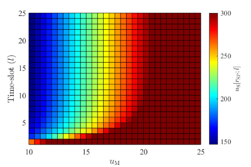
(a) $T_{\mathrm{b}}=1$ s

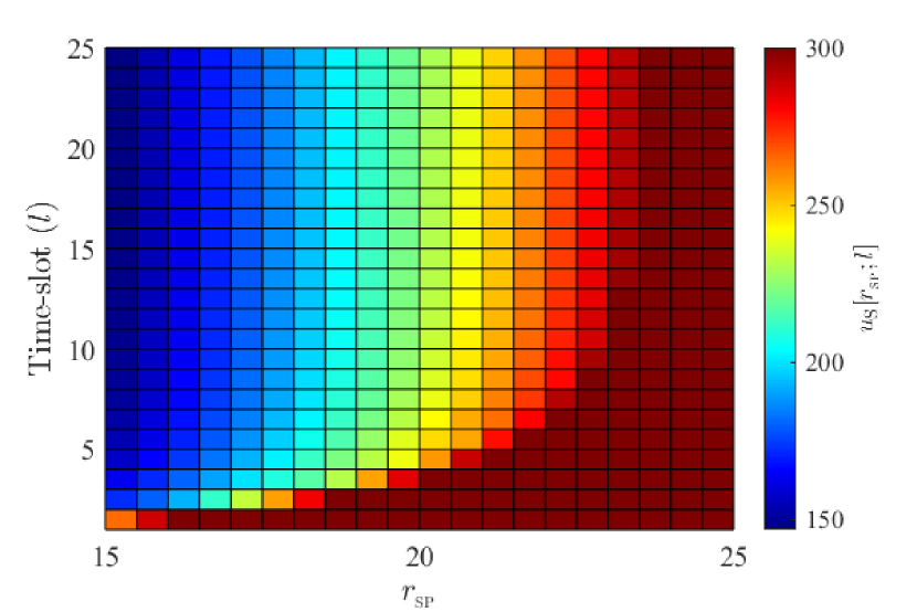
(b) $T_{\mathrm{b}}=1$ s

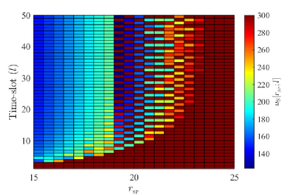
(c) $T_{\mathrm{b}}=0.4$ s

Figure 2: (a) Variation of $u_{{{}_{\mathrm{S}}}}[r_{{}_{\mathrm{SP}}};l]$ with the threshold $u_{\mathrm{M}}$ and time-slot $l$ when$\ r_{{}_{\mathrm{SP}}}=15\mu m$. (b) & (c) Variation of $u_{{{}_{\mathrm{S}}}}[r_{{}_{\mathrm{SP}}};l]$ with $r_{{}_{\mathrm{SP}}}$ and time-slot $l$ for different values of $T_{\mathrm{b}}$. Parameters: $D=100\mu m/s,\ u_{\mathrm{L}}=300$.

Fig. 2 (a) shows the variation of $u_{{{}_{\mathrm{S}}}}[r_{{}_{\mathrm{SP}}};l]$ with the interference threshold $u_{\mathrm{M}}$ at FAR_P, and time-slot $l$. When $u_{\mathrm{M}}$ decreases, the allowed interference at the FAR_P due to TX_S reduces, and $u_{{{}_{\mathrm{S}}}}[r_{{}_{\mathrm{SP}}};l]$ is decreased. Also, with the increase in the $l$, the ISI caused by the TX_S to the FAR_P increases, and the transmitted number of molecules $u_{{{}_{\mathrm{S}}}}[r_{{}_{\mathrm{SP}}};l]$ by the TX_P is reduced to limit the interference by $u_{\mathrm{M}}$. When $r_{{}_{\mathrm{SP}}}$ is small, the TX_S is near to FAR_P, resulting in high co-channel interference, and $u_{{{}_{\mathrm{S}}}}[r_{{}_{\mathrm{SP}}};l]$ is reduced to limit it. When $r_{{}_{\mathrm{SP}}}$ is large, the TX_S is far from FAR_P, resulting in low co-channel interference and $u_{{{}_{\mathrm{S}}}}[r_{{}_{\mathrm{SP}}};l]$ can be high. This trend can be seen in Fig. 2 (b). Also in Fig. 2 (a) and (b), $u_{{{}_{\mathrm{S}}}}[r_{{}_{\mathrm{SP}}};l]$ reaches a steady state value when $l$ is increased. $u_{{{}_{\mathrm{S}}}}[r_{{}_{\mathrm{SP}}};l]$ can be oscillatory also if $T_{\mathrm{b}}$ is too small, as seen in Fig. 2 (c).

Now to proceed further, we require $\mathrm{p}_{mi}\left({t,\mu}\right)$ i.e., the fraction of IM emitted by TX_m that are hitting the FAR_i in the presence of FAR${}_{\bar{i}}$ until time $t$ while considering the degradation of IMs which we do next.

IV Hitting Probability of an IM

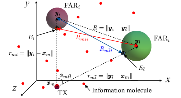
Figure 3: Schematic diagram of a 3-D diffusion based cognitive molecular communication system with a point transmitter and two spherical FARs.

We now analyze a system with one point transmitter (located at $\boldsymbol{x}_{m}$) and two FARs (located at $\boldsymbol{y}_{i}$ and $\boldsymbol{y}_{\bar{i}},\ i\in\{\mathrm{P},\mathrm{S}\}$) of unequal size (see Fig. 3) to derive an approximate expression for hitting probability of an IM at one of the FAR. We first consider the case with no molecular degradation and then extend the analysis for the case when molecular degradation is present. Note that an exact equation for a 3-D MCvD system with multiple fully-absorbing receivers is not available in the literature. The derived equation in this work is different than the one derived in [13], which considered FARs of the same size only.

IV-1 Without molecular degradation

Let $\mathrm{p}_{mi}\left({t}\right)=\mathrm{p}_{mi}\left({t,\mu=0}\right)$, $m,i\in\{\mathrm{P},\mathrm{S}\}$, denote the fraction of IMs (without degradation) absorbed within time $t$ by the FAR located at $\boldsymbol{y}_{i}$ in the presence of another FAR at $\boldsymbol{y}_{\bar{i}}$ when the transmitter is located at $\boldsymbol{x}_{m}$. This quantity is equal to the probability of an IM being absorbed by the FAR at $\boldsymbol{y}_{i}$ in the presence of other FAR at $\boldsymbol{y}_{j}$ until time $t$.

Theorem 1.

The closed-form approximate expression for $\mathrm{p}_{mi}\left({t}\right)$ can be derived as

$$\mathrm{p}_{mi}\left({t}\right)= \sum_{n=0}^{\infty}\left(\frac{a_{i}a_{{\bar{i}}}}{R_{mi{\bar{i}}}R_{m{\bar{i}}i}}\right)^{n}\left[\frac{a_{i}}{r_{mi}}\mathrm{erfc}\left(\frac{\Phi_{mi}(n)}{\sqrt{4Dt}}\right)\right.-\left.\frac{a_{i}a_{{\bar{i}}}}{r_{m{\bar{i}}}R_{m{\bar{i}}i}}\mathrm{erfc}\left(\frac{\Psi_{mi}(n)}{\sqrt{4Dt}}\right)\right],$$ (9)

where $\Phi_{mi}(n)=r_{mi}-a_{i}+n(R_{m{\bar{i}}i}{-}a_{i})+n(R_{mi{\bar{i}}}{-}a_{{\bar{i}}}),\ \Psi_{mi}(n)=r_{m{\bar{i}}}-a_{{\bar{i}}}+(n+1)(R_{m{\bar{i}}i}{-}a_{i})+n(R_{mi{\bar{i}}}{-}a_{{\bar{i}}})$ with $r_{mj}=\left\lVert\boldsymbol{y}_{j}-\boldsymbol{x}_{m}\right\rVert,\ j\in\{i,{\bar{i}}\}$ denoting the distance between the transmitter located at $\boldsymbol{x}_{m}$ and the intended FAR located at $\boldsymbol{y}_{j}$, and $R_{mi{\bar{i}}}^{2}=(r_{mi}-a_{i})^{2}+r_{m{\bar{i}}}^{2}-2(r_{mi}-a_{i})r_{m{\bar{i}}}\cos(\phi_{mi{\bar{i}}})$ denoting the square distance between the center of FAR${}_{\bar{i}}$ and the point at the surface of FAR_i, which closest to the transmitter ($E_{i}$). Here, $\phi_{mi{\bar{i}}}$ is the angle between the centers of FAR_i and FAR${}_{\bar{i}}$ when viewed from $\boldsymbol{x}_{m}$.

Proof:

See Appendix B. ∎

It is important to note that the error arising due to this approximation is small if (i) the distance between the TX_m and each FAR is significantly larger than the radius of the FAR i.e., $\left\lVert\boldsymbol{y}_{i}-\boldsymbol{x}_{m}\right\rVert\gg a_{i}$ and $\left\lVert\boldsymbol{y}_{\bar{i}}-\boldsymbol{x}_{m}\right\rVert\gg a_{{\bar{i}}}$, and (ii) the distance between the FARs is significantly larger than the maximum of the radius of FARs i.e., $R=\left\lVert\boldsymbol{y}_{i}-\boldsymbol{y}_{\bar{i}}\right\rVert\gg\max{\left(a_{{}_{\mathrm{P}}},a_{{}_{\mathrm{S}}}\right)}$ as verified in Fig. 5.

Corollary 1.1.

The fraction of IMs with eventually hitting FAR_i is

$$\mathrm{p}_{mi}\left({\infty}\right)=\frac{a_{i}R_{mi{\bar{i}}}}{R_{mi{\bar{i}}}R_{m{\bar{i}}i}-a_{i}a_{{\bar{i}}}}\left[\frac{R_{m{\bar{i}}i}}{r_{mi}}-\frac{a_{{\bar{i}}}}{r_{m{\bar{i}}}}\right].$$ (10)

The hitting rate of molecules on the FAR located at $\boldsymbol{y}_{i}$ in the presence of other FAR at time $\tau$ can be derived by taking the derivative of (9) with respect to $t$. That is,

$$\kappa_{mi}\left({\tau}\right)=\sum_{n=0}^{\infty}\left(\frac{a_{i}a_{{\bar{i}}}}{R_{mi{\bar{i}}}R_{m{\bar{i}}i}}\right)^{n} \left[\frac{a_{i}}{r_{mi}}\frac{\Phi_{mi}(n)}{\sqrt{4\pi D\tau^{3}}}\exp\left(-\frac{\Phi_{mi}(n)^{2}}{4D\tau}\right)\right.$$

$$-\left.\frac{a_{i}a_{{\bar{i}}}}{r_{m{\bar{i}}}R_{m{\bar{i}}i}}\frac{\Psi_{mi}(n)}{\sqrt{4\pi D\tau^{3}}}\exp\left(-\frac{\Psi_{mi}(n)^{2}}{4D\tau}\right)\right].$$ (11)

IV-2 With molecular degradation

We now consider degradable IMs with exponential degradation where the probability that a molecule will not degrade over time $t$ is, $\exp{\left(-\mu t\right)}$. Here, $\mu$ denotes the reaction rate constant of molecular degradation which is related to the half-time as $\mu=\ln(2)/\Lambda_{1/2}$. When the reaction rate tends to zero ($\mu\rightarrow 0$, i.e. half-time is infinity $\Lambda_{1/2}\rightarrow\infty$), the molecule will never undergo degradation. We also assume that the molecule does not get involved in any other reactions.

Now, using the exponential distribution for molecular life expectancy, the fraction of non-degraded IMs reaching the FAR_i in the presence of the other FAR within time $t$, due to the emission of IMs from the transmitter at $\boldsymbol{x}_{m}$ is given by

$$\mathrm{p}_{mi}\left({t,\mu}\right)= \int_{0}^{t}\kappa_{mi}\left({\tau}\right)\exp\left(-\mu\tau\right)\mathrm{d}\tau.$$ (12)

Further, substituting (11) in (12), the closed-form approximate expression for hitting probability can be derived as presented in Theorem 2 below.

Theorem 2.

The probability of a non-degraded IM hitting the FAR located at $\boldsymbol{y}_{i}$ within time $t$, due to the emission from the transmitter at $\boldsymbol{x}_{m}$ in the presence of the other FAR is

$$\mathrm{p}_{mi}\left({t,\mu}\right)=\sum_{n=0}^{\infty}\left(\frac{a_{i}a_{{\bar{i}}}}{R_{mi{\bar{i}}}R_{m{\bar{i}}i}}\right)^{n}\left[\frac{a_{i}}{r_{mi}}f(\Phi_{mi}(n))-\frac{a_{i}a_{{\bar{i}}}}{r_{m{\bar{i}}}R_{m{\bar{i}}i}}f(\Psi_{mi}(n))\right],$$ (13)

where

$$f(x)= \frac{1}{2}\left[\mathrm{erfc}\left(\frac{x}{\sqrt{4Dt}}{+}\sqrt{\mu t}\right)\exp\left(x\sqrt{\frac{\mu}{D}}\right)\right.\left.+\mathrm{erfc}\left(\frac{x}{\sqrt{4Dt}}{-}\sqrt{\mu t}\right)\exp\left({-}x\sqrt{\frac{\mu}{D}}\right)\right].$$

Proof:

See Appendix C. ∎

Corollary 2.1.

$\lim\limits_{\mu\rightarrow 0}\mathrm{p}_{mi}\left({t,\mu}\right)=\mathrm{p}_{mi}\left({t}\right)$.

Corollary 2.2.

The fraction of IMs eventually hitting FAR_i is

$$\mathrm{p}_{mi}\left({\infty,\mu}\right)=\frac{a_{i}R_{mi{\bar{i}}}}{R_{mi{\bar{i}}}R_{m{\bar{i}}i}-a_{i}a_{{\bar{i}}}\exp\left(-\left(R_{mi{\bar{i}}}+R_{m{\bar{i}}i}-a_{i}-a_{{\bar{i}}}\right)\sqrt{\frac{\mu}{D}}\right)}$$

$$\ \ \ \ \ \ \ \ \ \ \ \ \times\left[\frac{R_{m{\bar{i}}i}}{r_{mi}}\exp\left(-\left(r_{mi}-a_{i}\right)\sqrt{\frac{\mu}{D}}\right)\right.\left.-\frac{a_{{\bar{i}}}}{r_{m{\bar{i}}}}\exp\left(-\left(r_{m{\bar{i}}}-a_{{\bar{i}}}+R_{m{\bar{i}}i}-a_{i}\right)\sqrt{\frac{\mu}{D}}\right)\right].$$ (14)

Proof:

When $t\rightarrow\infty$, (13) gives

$$\mathrm{p}_{mi}\left({\infty,\mu}\right)= \sum_{n=0}^{\infty}\left(\frac{a_{i}a_{{\bar{i}}}}{R_{mi{\bar{i}}}R_{m{\bar{i}}i}}\right)^{n}\left[\frac{a_{i}}{r_{mi}}\exp\left(-\Phi_{mi}(n)\sqrt{\frac{\mu}{D}}\right)\right.\left.-\frac{a_{i}a_{{\bar{i}}}}{r_{m{\bar{i}}}R_{m{\bar{i}}i}}\exp\left(-\Psi_{mi}(n)\sqrt{\frac{\mu}{D}}\right)\right].$$ (15)

Simplifying (15) further gives (14). ∎

IV-A Validation of Hitting Probability Equation of a System With Two FARs

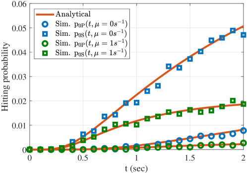
Figure 4: Hitting probability versus time for different degradation rate constant. Parameters: $D=100\mu m/s,\ \boldsymbol{x}_{m}=[0,0,0],\ \boldsymbol{y}_{{}_{\mathrm{P}}}=[-30,-20,0],\ \boldsymbol{y}_{{}_{\mathrm{S}}}=[25,10,0],\ D=100\mu m/s,\ a_{{}_{\mathrm{P}}}=3\mu m,\ a_{{}_{\mathrm{S}}}=5\mu m,\ \Delta t=10^{-4}s.$

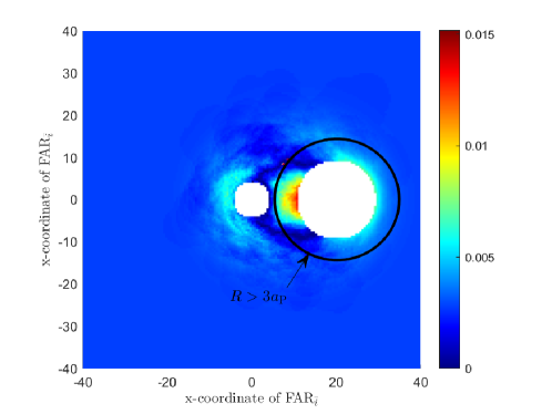
Figure 5: Approximation error in the hitting probability of IM on FAR_i located at $\boldsymbol{y}_{i}=[20,0,0]$ in the presence of FAR${}_{\bar{i}}$ in $\mathbb{R}^{3}$. Parameters: $\boldsymbol{x}_{m}=[0,0,0],\ D=100\mu m/s,\ a_{{}_{\mathrm{P}}}=5\mu m,\ a_{{}_{\mathrm{S}}}=4\mu m,\ \Delta t=10^{-4}s,\ t=1s$.

The approximate analytical expressions (9) and (13) derived are validated using particle based simulations in Fig. 4. The step size $\Delta t$ chosen for the simulation is $10^{-4}$s. The transmitter is assumed to be located at the origin, i.e., $\ \boldsymbol{x}_{m}=[0,0,0]$. The FAR_P is located at $\boldsymbol{y}_{{}_{\mathrm{P}}}=[-30,-20,0]$ and the FAR_S is located at $\boldsymbol{y}_{{}_{\mathrm{S}}}=[25,10,0]$. It is evident from the Fig. 4 that, the derived approximate analytical expressions considering and without considering molecular degradation are in good match with the particle-based simulation results for the chosen parameters.

The accuracy of approximating the hitting point of an IM on FAR_i by $E_{i}$ can be observed in Fig. 5, which shows the absolute error ($|\text{Exact value-Analytical value}|$) when FAR_i is at a fixed location, while FAR${}_{\bar{i}}$ is moved in $\mathbb{R}^{3}$. It can be seen that the absolute error is negligible when $R=\left\lVert\boldsymbol{y}_{i}-\boldsymbol{y}_{\bar{i}}\right\rVert>3a_{{}_{\mathrm{P}}}$. The low values of absolute error guarantee the accuracy of the derived equations.

The derived approximate hitting probability expressions are used to model and analyze the underlay cognitive molecular communication system discussed in the upcoming sections. We now incorporate this derived result to evaluate the performance of the cognitive system.

V Expected number of absorbed molecules

In this section, we derive the expected number of molecules absorbed at the FAR_P and FAR_S at the $l$th time-slot.

The total number of molecules absorbed at the FAR_P on $l$th slot is $z_{{}_{\mathrm{P}}}[l]$. Therefore the expected total number of molecules absorbed at the FAR_P is

$$\mathbb{E}\left[z_{{}_{\mathrm{P}}}[l]\right] =Nq_{{}_{1\mathrm{P}}}\sum_{k=1}^{l}h_{{}_{\mathrm{PP}}}[l-k]+q_{{}_{1\mathrm{S}}}\sum_{k=1}^{l}u_{{{}_{\mathrm{S}}}}[r_{{}_{\mathrm{SP}}};k]h_{{}_{\mathrm{SP}}}[l-k]$$

$$=Nq_{{}_{1\mathrm{P}}}\mathrm{p}_{{{}_{\mathrm{PP}}}}\left({lT_{\mathrm{b}},\mu}\right)+q_{{}_{1\mathrm{S}}}\sum_{k=1}^{l}u_{{{}_{\mathrm{S}}}}[r_{{}_{\mathrm{SP}}};k]h_{{}_{\mathrm{SP}}}[l-k].$$ (16)

Similarly, the total number of molecules absorbed at the FAR_S on $l$th slot is $z_{{}_{\mathrm{S}}}[l]$. Therefore the expected total number of molecules absorbed at the FAR_S is

$$\mathbb{E}\left[z_{{}_{\mathrm{S}}}[l]\right]=Nq_{{}_{1\mathrm{P}}}\mathrm{p}_{{{}_{\mathrm{PS}}}}\left({lT_{\mathrm{b}},\mu}\right)+q_{{}_{1\mathrm{S}}}\sum_{k=1}^{l}u_{{{}_{\mathrm{S}}}}[r_{{}_{\mathrm{SP}}};k]h_{{}_{\mathrm{SS}}}[l-k].$$ (17)

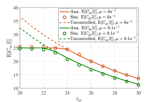
Figure 6: Variation of the expected number of absorbed molecules at the FAR_P due to the emission from TX_S with respect to $r_{{}_{\mathrm{SP}}}$. Initial position of TX_S is $\boldsymbol{x}_{{}_{\mathrm{S}}}=[0,0,0]$. TX_S is shifted in positive x axis direction. Parameters: $D=100\mu m/s,\ l=3,u_{\mathrm{M}}=25,u_{L}=1000,\boldsymbol{x}_{{}_{\mathrm{P}}}=[55,0,0],\ \boldsymbol{y}_{{}_{\mathrm{P}}}=[30,0,0],\ \boldsymbol{y}_{{}_{\mathrm{S}}}=[30,50,0]$.

Fig. 6 shows the variation of the expected number of absorbed molecules at the FAR_P due to the emission from TX_S ($\mathbb{E}\left[C_{{}_{\mathrm{SP}}}[l]\right]$) with respect to $r_{{}_{\mathrm{SP}}}$. When $r_{{}_{\mathrm{SP}}}$ is small, the interference from the TX_S to the FAR_P is high, and $u_{{{}_{\mathrm{S}}}}[r_{{}_{\mathrm{SP}}};l]$ is adapted (as in eq. (6)) at the TX_S to limit the allowed interference to $u_{\mathrm{M}}$ molecules at FAR_P. When $r_{{}_{\mathrm{SP}}}$ increases, the expected number of interfering molecules observed at the FAR_P falls below $u_{\mathrm{M}}$ due to the lossy channel. If $u_{{{}_{\mathrm{S}}}}[r_{{}_{\mathrm{SP}}};l]$ is uncontrolled ($u_{{{}_{\mathrm{S}}}}[r_{{}_{\mathrm{SP}}};l]=1000$, represented by dashed lines in Fig. 6.) the co-channel interference at the FAR_P keep on increasing when $r_{{}_{\mathrm{SP}}}$ decreases. Also, when the molecular degradation rate increases, $\mathbb{E}\left[C_{{}_{\mathrm{SP}}}[l]\right]$ falls due to the degradation of molecules.

In the following section, we derive the novel closed-form expressions for the probability of bit error to analyze the performance at FAR_P and FAR_S.

VI Analysis of the Probability of Bit Error

At the end of $l$th time-slot, the number of IMs absorbed ($z_{i}[l],\ i\in\{\mathrm{P},\mathrm{S}\}$) at each FAR is compared with the threshold $\eta[i;l]$ for decoding the bit $b_{i}[l]$ transmitted by the TX_i at the beginning of $l$th time-slot. If $z_{i}[l]<\eta[i;l]$, then the transmitted bit $b_{i}[l]$ is estimated as $\hat{b}_{i}[l]=0$, otherwise $\hat{b}_{i}[l]=1$. An error occurs when the transmitted bit $b_{i}[l]=0$ is decoded as $\hat{b}_{i}[l]=1$ and vice versa. Thus, the total probability of bit error ($\mathrm{P}_{\mathrm{e}i}$) is given by

$$\mathrm{P}_{\mathrm{e}i}[l]= \mathbb{P}\left[b_{i}[l]=0\right]\mathrm{P}_{\mathrm{e}i,0}[l]+\mathbb{P}\left[b_{i}[l]=1\right]\mathrm{P}_{\mathrm{e}i,1}[l],$$ (18)

where $\mathrm{P}_{\mathrm{e}i,0}[l]$ and $\mathrm{P}_{\mathrm{e}i,1}[l],i\in\{\mathrm{P},\mathrm{S}\}$ are the probabilities of incorrect decoding for bit 0 and 1, respectively, and are defined as

$$\mathrm{P}_{\mathrm{e}i,0}[l] =\mathbb{P}\left[\hat{b}_{i}[l]=1\mid b_{i}[l]=0\right],$$

$$\mathrm{P}_{\mathrm{e}i,1}[l] =\mathbb{P}\left[\hat{b}_{i}[l]=0\mid b_{i}[l]=1\right].$$ (19)

To derive the closed-form expression for $\mathrm{P}_{\mathrm{e}i,0}[l]$ and $\mathrm{P}_{\mathrm{e}i,1}[l]$, we employ the moment generating function approach and the results are presented in Theorem 3.

VI-A Probability of Bit Error at FAR_P and FAR_S

Theorem 3.

The probability of bit error at the receiver $i\in\{\mathrm{P},\mathrm{S}\}$ given by (18) with the probability of incorrect decoding for bit 1 and 0 given as

$$\mathrm{P}_{\mathrm{e}i,1}[l]= \sum_{n=0}^{\eta[i;l]-1}\sum_{\begin{subarray}{c}n_{0}+n_{1}+\cdots+n_{2l-1}=n\\ n_{s}<u_{\bar{i}}(2l-s),\ \forall l\leq s\leq 2l-1\end{subarray}}\!\!\frac{1}{n_{0}!n_{1}!\cdots n_{2l-1}!}\beta_{i}^{(n_{0})}(l)\prod_{r=1}^{l-1}\alpha_{ii}^{(n_{r})}(r)\prod_{s=l}^{2l-1}\alpha_{i{\bar{i}}}^{(n_{s})}(s-l),$$ (20)

and

$$\mathrm{P}_{\mathrm{e}i,0}[l]=1- \sum_{n=0}^{\eta[i;l]-1}\sum_{\begin{subarray}{c}n_{1}+n_{2}+\cdots+n_{2l-1}=n\\ n_{s}<u_{\bar{i}}(2l-s),\ \forall l\leq s\leq 2l-1\end{subarray}}\frac{1}{n_{1}!n_{2}!\cdots n_{2l-1}!}\prod_{r=1}^{l-1}\alpha_{ii}^{(n_{r})}(r)\prod_{s=l}^{2l-1}\alpha_{i{\bar{i}}}^{(n_{s})}(s-l),$$ (21)

where the second sum extends over all $n_{0},n_{1},\cdots,n_{2l-1}$ of non-negative integers such that $n_{0}+n_{1}+\cdots+n_{2l-1}=n$. The variables $\alpha_{ij}^{(k)}(s)$ for $\ j\in\{i,{\bar{i}}\}$ and $\beta_{i}^{(k)}(l)$ are defined as,

$$\alpha_{ij}^{(k)}(s)= q_{{}_{0j}}\mathbbm{1}(k=0)+q_{{}_{1j}}\left(1-h_{ji}[s]\right)^{u_{j}(l-s)-k}\times h_{ji}[s]^{k}\frac{u_{j}(l-s)!}{\left(u_{j}(l-s)-k\right)!},$$ (22)

and

$$\beta_{i}^{(k)}(l)= \frac{1}{q_{{}_{1i}}}\left(\alpha_{ii}^{(k)}(l)-q_{{}_{0i}}\mathbbm{1}(k=0)\right),$$ (23)

where $u_{{}_{\mathrm{P}}}(s)=N$ and $u_{{}_{\mathrm{S}}}(s)=u_{{}_{\mathrm{S}}}\left[r_{{}_{\mathrm{SP}}};s\right]$ (with some abuse of notation).

Proof:

See Appendix D. ∎

Remark 4.

Consider the FAR_P probability of bit error performance with the variation in the distance between FAR_P and TX_S. When the TX_S moves closer to the FAR_P, $h_{{}_{\mathrm{SP}}}[s-l]$ in (22) increases and $\mathrm{P}_{\mathrm{e}{{}_{\mathrm{P}}}}[l]$ increases due to the increase in $\alpha_{i{\bar{i}}}^{(k)}(s)$ if the transmitted molecules at the TX_S is not controlled. However, for in controlled transmission, an increase in $h_{{}_{\mathrm{SP}}}[s-l]$ is counteracted by a corresponding decrease in $u_{{{}_{\mathrm{S}}}}[r_{{}_{\mathrm{SP}}};2l-s]$ to reduce the rise in $\mathrm{P}_{\mathrm{e}{{}_{\mathrm{P}}}}[l]$.

Corollary 3.1.

Assuming $\eta=1$ and the probability of sending bit $0$ and $1$ as $1/2$, the total probability of error at the $i$th receiver is

$$\mathrm{P}_{\mathrm{e}i}[l]=0.5\left(1+\prod_{r=1}^{l-1}a_{ii}^{(0)}(r)\prod_{s=l+1}^{2l}\alpha_{i{\bar{i}}}^{(0)}(s-l)\left[\beta_{i}^{(0)}(l)-1\right]\right).$$ (24)

From the above equation, we can verify that the second term with product terms is negative and with the increase in ISI, the value of the second term reduces and $\mathrm{P}_{\mathrm{e}i}[l]$ increases.

Corollary 3.2.

For a system without ISI, the probability of bit error at the FAR${}_{i},\ i\in\{\mathrm{P},\mathrm{S}\}$ is given by

$$\mathrm{P}_{\mathrm{e}i}[l]= q_{{}_{1i}}\sum_{n=0}^{\eta[i;l]-1}\frac{1}{n!}\sum_{k=0}^{n}\!\!{n\choose k}\beta_{i}^{(n-k)}(l)\alpha_{i{\bar{i}}}^{(k)}(l)+q_{{}_{0i}}\left[1-\sum_{n=0}^{\eta[i;l]-1}\frac{1}{n!}\alpha_{i{\bar{i}}}^{(n)}(l)\right].$$ (25)

VI-B Effect of Threshold on Probability of Bit Error

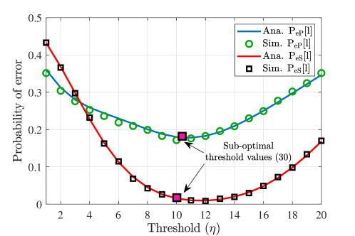
Figure 7: Variation of the probability of bit error with respect to threshold $\eta$. Parameters: $D=100\mu m/s,\ a_{{}_{\mathrm{P}}}=3\mu m,a_{{}_{\mathrm{S}}}=5\mu m,T_{\mathrm{b}}=2s,l=3,u_{\mathrm{M}}=5,u_{\mathrm{L}}=300,\mu=0.5s^{-1},\ \boldsymbol{x}_{{}_{\mathrm{P}}}{=}[30,-10,0],\ \boldsymbol{x}_{{}_{\mathrm{S}}}{=}[10,10,0],\ \boldsymbol{y}_{{}_{\mathrm{P}}}=[30,10,0],\ \boldsymbol{y}_{{}_{\mathrm{S}}}=[10,10,20]$.

Fig. 7 shows the variation of probability of bit error with the threshold for detection $\eta$ at the FAR_P and the FAR_S. With the increase in $\eta$, the probability of bit error first reduces until it reaches the minimum point and then starts increasing. Therefore, there exists an optimal threshold for which the probability of bit error is minimum. In Fig. 7, the probability of bit error at the FAR_P is higher than that of FAR_S since the size of FAR_P is smaller, and thereby the hitting probability is smaller compared to that of FAR_S.

It is evident from Fig. 7 that the detection threshold plays a vital role in determining the performance of the system and must be chosen correctly to increase system performance which we study next.

VI-C Detection threshold $\eta[i;l]$

The probability of bit error derived in Theorem 3 varies significantly with the threshold of detection as seen in Fig. 7. The communication will be effective when the detection threshold is chosen such that the probability of bit error is minimum. Threshold for which the probability of bit error is minimum is termed as optimum threshold. In this section, we derive the sub-optimum threshold for detection at the FAR_P and FAR_S.

Now, for decoding at the FAR_i, we can chose the null hypothesis $\mathcal{H}_{0i}[l]$ and alternative hypothesis $\mathcal{H}_{1i}[l]$ as the event of sending bit $0$ and $1$ respectively by the TX_i. The decision rule at the $i$th receiver is

$$z_{i}[l]\overset{\mathcal{H}_{1i}}{\underset{\mathcal{H}_{0i}}{\gtrless}}\eta[i;l].$$ (26)

The calculation of $\eta[i;l],\ i\in\{\mathrm{P},\mathrm{S}\}$ is complex since the received number of molecules are Binomial distributed. For tractability, Binomial random variables $z_{i{\bar{i}}}[l;k]\sim\mathcal{B}\left(b_{i}[k]u_{i}[k],h_{i{\bar{i}}}[l-k]\right),\ 1\leq k\leq l,\ i\in\{\mathrm{P},\mathrm{S}\},u_{i}[k]\in\{N,u_{{{}_{\mathrm{S}}}}[r_{{}_{\mathrm{SP}}};k]\}$ can be approximated to Poisson random variable $z_{i{\bar{i}}}[l;k]\sim\mathcal{P}\left(b_{i}[k]u_{i}[k]h_{i{\bar{i}}}[l-k]\right)$ [21].

Using the Poisson approximation of $z_{i{\bar{i}}}[l;k]$, the mean number of molecules absorbed at the FAR_i at the $l$th time-slot when the transmitted bit is $0$ and $1$ are

$$\lambda_{0i}[l]=Nq_{{}_{1i}}\sum_{k=1}^{l-1}u_{i}[k]h_{ii}[l-k]+q_{{}_{1{\bar{i}}}}\sum_{k=1}^{l}u_{\bar{i}}[k]h_{{\bar{i}}i}[l-k],$$ (27)

and

$$\lambda_{1i}[l]=u_{i}[l]h_{ii}[0]+\lambda_{0i},$$ (28)

respectively. For finding the sub-optimum decision threshold at receivers, the log-likelihood ratio test (LLRT) can be used,

$$\ln\left[\frac{\mathrm{P}\left(z_{i}[l]\mid\mathcal{H}_{1i}[l]\right)}{\mathrm{P}\left(z_{i}[l]\mid\mathcal{H}_{0i}[l]\right)}\right]\overset{\mathcal{H}_{1i}}{\underset{\mathcal{H}_{0i}}{\gtrless}}\ln\left[\frac{q_{{}_{0i}}}{q_{{}_{1i}}}\right],$$ (29)

where

$$\mathrm{P}\left(z_{i}[l]\mid\mathcal{H}_{1i}[l]\right)=e^{-\lambda_{1i}[l]}\frac{\lambda_{1i}[l]^{z_{i}[l]}}{z_{i}[l]!},$$

and

$$\mathrm{P}\left(z_{i}[l]\mid\mathcal{H}_{0i}[l]\right)=e^{-\lambda_{0i}[l]}\frac{\lambda_{0i}[l]^{z_{i}[l]}}{z_{i}[l]!}.$$

Now, solving (29) and comparing with (26) gives [22]

$$\eta[i;l]=\frac{\ln\left(q_{{}_{0i}}/q_{{}_{1i}}\right)+h_{ii}[0]u_{i}[l]}{\ln\left(\lambda_{1i}[l]/\lambda_{0i}[l]\right)}.$$ (30)

The detection threshold value derived in (30) is the sub-optimal threshold for the FAR_P and FAR_S at the $l$th time-slot. It is evident from Fig. 7 that, the sub-optimal values obtained in (30) is close to the optimal threshold values. The derived value of detection threshold is sub-optimal since it is calculated based on the average value instead of instantaneous values.

VI-D Effect of Fixed and Variable Threshold on Probability of Bit Error

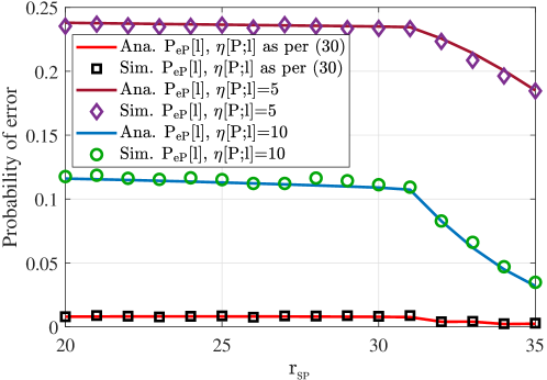
Figure 8: Variation of the probability of bit error with respect to $r_{{}_{\mathrm{SP}}}$ when $\eta[i;l]$ is varying as in (30) or fixed. Parameters: $D=100\mu m/s,\ a_{{}_{\mathrm{P}}}=5\mu m,\ a_{{}_{\mathrm{S}}}=5\mu m,\ T_{\mathrm{b}}=5s,\ l=3,\ u_{\mathrm{M}}=5,\ u_{L}=300,\ \boldsymbol{x}_{{}_{\mathrm{P}}}=[30,-10,0],\ \boldsymbol{y}_{{}_{\mathrm{P}}}=[30,10,0],\ \boldsymbol{y}_{{}_{\mathrm{S}}}=[10,10,20]$. The initial location of $\boldsymbol{x}_{{}_{\mathrm{S}}}=[0,10,0]$ and it is varied in positive $x-$ axis.

Fig. 8 shows the variation of probability of bit error at the FAR_P with respect to $r_{{}_{\mathrm{SP}}}$ for fixed $\eta$ and sub-optimal $\eta[i;l]$ values. The probability of bit error is minimum when the $\eta[i;l]$ values are optimally controlled. Fixed values of $\eta$ result in a higher probability of bit error. When $r_{{}_{\mathrm{SP}}}$ is high, the co-channel interference molecules reaching the FAR_P is less than the maximum allowable interference $u_{\mathrm{M}}$. When $r_{{}_{\mathrm{SP}}}$ reduces, co-channel interference increases and reaches $u_{\mathrm{M}}$ eventually, thereby maintaining the probability of bit error constant afterward.

VI-E Effect of $r_{{}_{\mathrm{SP}}}$ on Probability of Bit Error

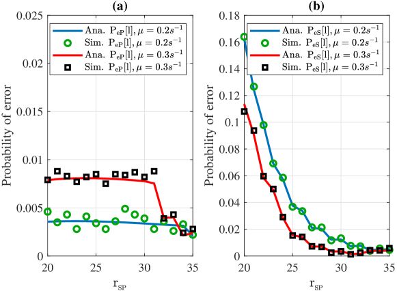
Figure 9: Variation of the probability of bit error with respect to $r_{{}_{\mathrm{SP}}}$ for different degradation values. Parameters: $D=100\mu m/s,\ a_{{}_{\mathrm{P}}}=5\mu m,a_{{}_{\mathrm{S}}}=5\mu m,T_{\mathrm{b}}=5s,l=3,u_{\mathrm{M}}=5,u_{L}=300,\ \boldsymbol{x}_{{}_{\mathrm{P}}}=[30,-10,0],\ \boldsymbol{y}_{{}_{\mathrm{P}}}=[30,10,0],\ \boldsymbol{y}_{{}_{\mathrm{S}}}=[10,10,20],\ \eta[i;l]=\text{as per \eqref{opt_thr}}$. The initial location of $\boldsymbol{x}_{{}_{\mathrm{S}}}=[0,10,0]$ and it is varied in positive $x-$ axis

Fig. 9 shows the variation of probability of bit error with the distance between TX_S and FAR_P ($r_{{}_{\mathrm{SP}}}$) for two different values of molecular degradation rate constant. When $r_{{}_{\mathrm{SP}}}$ decreases, the co-channel interference at the FAR_P increases and the probability of bit error rises. However, due to the controlling of the transmitted number of molecules by the TX_S, the co-channel interference is limited to $u_{\mathrm{M}}$, and the probability of bit error remains unaffected. Nevertheless, due to this restriction, when $r_{{}_{\mathrm{SP}}}$ reduces, $u_{{{}_{\mathrm{S}}}}[r_{{}_{\mathrm{SP}}};l]$ reduces, and the probability of bit error at FAR_S increases. Therefore, for the cognitive pair to work with good performance, TX_S should be far from FAR_P.

When molecular degradation is faster, the primary and secondary link performance changes in different ways, as seen in Fig. 9 (a) and (b). For the chosen parameters, TX_P to FAR_P distance and TX_S to FAR_S distance is less than TX_P to FAR_S distance and TX_S to FAR_P distance. Therefore co-channel interference molecules are more prone to degradation. Secondary link performance improves with degradation because the number of interfering molecules to FAR_P degrades more. Due to this, TX_S can send more molecules to FAR_S without crossing the co-interference beyond the desired limit of $u_{\mathrm{M}}$. For the primary link, the co-channel interference does not change with $\mu$ when FAR_P and TX_S are nearby, but at the same time, the desired molecules emitted by TX_P to FAR_P degrades in a small amount. This results in the slight diminishing of bit error performance when $\mu$ is increased.

VI-F Effect of Controlled Transmission on Probability of Bit Error

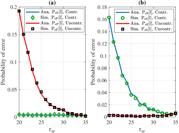
Figure 10: Variation of the probability of bit error with respect to $r_{{}_{\mathrm{SP}}}$ when $u_{{{}_{\mathrm{S}}}}[r_{{}_{\mathrm{SP}}};l]$ is controlled and uncontrolled. Parameters: $D=100\mu m/s,\ a_{{}_{\mathrm{P}}}=5\mu m,\ a_{{}_{\mathrm{S}}}=5\mu m,T_{\mathrm{b}}=5s,l=3,u_{\mathrm{M}}=5,u_{L}=300,\ \boldsymbol{x}_{{}_{\mathrm{P}}}=[30,-10,0],\ \boldsymbol{y}_{{}_{\mathrm{P}}}=[30,10,0],\ \boldsymbol{y}_{{}_{\mathrm{S}}}=[10,10,20],\ \eta[i;l]=\text{as per \eqref{opt_thr}}$. The initial location of $\boldsymbol{x}_{{}_{\mathrm{S}}}=[0,10,0]$ and it is varied in positive $x-$ axis.

Fig. 10 shows the effect of the control of molecules emitted by the TX_S on the bit error probability. In the controlled emission of the molecules from the TX_S, molecule emission is controlled according to $r_{{}_{\mathrm{SP}}}$ as in (6) for bit 1 transmission. However, for uncontrolled emission the TX_S emits a fixed number (here $u_{{{}_{\mathrm{S}}}}[r_{{}_{\mathrm{SP}}};l]=300$ molecules) of molecules for bit 1 transmission. Fig. 10 (a) and (b) validates that the controlling of molecules emitted by the TX_S based on $r_{{}_{\mathrm{SP}}}$ helps to maintains good performance to the high priority primary link. In contrast, the lower priority cognitive link performance deteriorates when $r_{{}_{\mathrm{SP}}}$ reduces.

VII Conclusions

In this work, we consider a cognitive molecular communication system with an underlay strategy for the co-existence of two communication links with different priorities. Each link has a point transmitter and spherical fully-absorbing receiver communicating with the same type of molecules. The transmitted number of molecules by the low priority secondary transmitter is controlled to limit its co-channel interference to the high priority primary link. We first derive an approximate equation for the information molecule hitting probability on each of the spherical fully-absorbing receivers with different sizes. We include the impact of molecular degradation in our analysis. The derived equation is used to develop an analytic framework for the cognitive molecular communication. The underlay strategy of cognitive molecular communication is studied, and several essential insights have been presented in this work.

Appendix A Proof of Remark 3

Recall that, the average number of interfering molecules should not exceed an acceptable threshold $u_{\mathrm{M}}$. At the steady state,

$$\mathbb{E}\left[C_{{}_{\mathrm{SP}}}[\infty]\right]=\mathbb{E}\left[\sum_{k=1}^{\infty}z_{{}_{\mathrm{SP}}}[l;k]\right]\leq u_{\mathrm{M}}.$$ (31)

The $\mathbb{E}\left[C_{{}_{\mathrm{SP}}}[\infty]\right]$ in above expression can be further solved as

$$\mathbb{E}\left[C_{{}_{\mathrm{SP}}}[\infty]\right] =\sum_{k=1}^{\infty}\mathbb{E}\left[z_{{}_{\mathrm{SP}}}[l;k]\right]$$

$$=q_{{}_{1\mathrm{S}}}u_{{{}_{\mathrm{S}}}}[r_{{}_{\mathrm{SP}}};\infty]\sum_{k=0}^{\infty}h_{{}_{\mathrm{SP}}}[k]$$

$$=q_{{}_{1\mathrm{S}}}u_{{{}_{\mathrm{S}}}}[r_{{}_{\mathrm{SP}}};\infty]\mathrm{p}_{{{}_{\mathrm{S}}}{{}_{\mathrm{P}}}}\left({\infty,\mu}\right).$$ (32)

Comparing (31) and (32) gives (8).

Appendix B Proof of Theorem 1

The probability that the IM emitted by the point source located at $\boldsymbol{x}_{m}$ reaches FAR${}_{\bar{i}}$ in the interval $[\tau,\ \tau+\mathrm{d}\tau]$ is $\left[\frac{\partial\mathrm{p}_{m{\bar{i}}}\left({\tau}\right)}{\partial\tau}\right]\mathrm{d}\tau$. The probability that this IM hits the FAR_i in the remaining time $t-\tau$ is $\overline{\mathrm{p}}\left({t-\tau,a,R_{m{\bar{i}}i}}\right)$, where $R_{m{\bar{i}}i}$ is the distance between the nearest point on the surface of FAR${}_{\bar{i}}$ from the transmitter (located at $\boldsymbol{x}_{m}$) and the center of FAR_i ($E_{\bar{i}}$ as seen in Fig. 3). Here the initial location of IM generation after the hit at FAR${}_{\bar{i}}$ is approximated as the nearest point on the surface of FAR${}_{\bar{i}}$ ($E_{\bar{i}}$) from the transmitter. The probability of an IM that is supposed to hit the FAR_i within time $t$ but is hitting FAR${}_{\bar{i}}$ instead is

$$\overline{\mathrm{p}}\left({t,a_{i},r_{mi}}\right){-}\mathrm{p}_{mi}\left({t}\right){=}\int_{0}^{t}\frac{\partial\mathrm{p}_{m{\bar{i}}}\left({\tau}\right)}{\partial\tau}\overline{\mathrm{p}}\left({t-\tau,a_{i},R_{m{\bar{i}}i}}\right)\mathrm{d}\tau.$$ (33)

Similarly, the probability of an IM that is supposed to hit the FAR_j with in time $t$ but is hitting the FAR_i is

$$\overline{\mathrm{p}}\left({t,a_{{\bar{i}}},r_{m{\bar{i}}}}\right){-}\mathrm{p}_{m{\bar{i}}}\left({t}\right)=\int_{0}^{t}\frac{\partial\mathrm{p}_{mi}\left({\tau}\right)}{\partial\tau}\overline{\mathrm{p}}\left({t-\tau,a_{{\bar{i}}},R_{mi{\bar{i}}}}\right)\mathrm{d}\tau.$$ (34)

Now, taking the Laplace transform of (33) and (34) gives

$$\overline{\mathcal{P}}\left({s,a_{i},r_{mi}}\right){-}\mathcal{P}_{mi}\left({s}\right){=}s\mathcal{P}_{m{\bar{i}}}\left({s}\right)\overline{\mathcal{P}}\left({s,a_{i},R_{m{\bar{i}}i}}\right)$$ (35)

and

$$\overline{\mathcal{P}}\left({s,a_{{\bar{i}}},r_{m{\bar{i}}}}\right){-}\mathcal{P}_{m{\bar{i}}}\left({s}\right){=}s\mathcal{P}_{mi}\left({s}\right)\overline{\mathcal{P}}\left({s,a_{{\bar{i}}},R_{mi{\bar{i}}}}\right)$$ (36)

Note that [23],

$$\overline{\mathrm{p}}\left({t,x,y}\right)=\frac{x}{y}\mathrm{erfc}\left(\frac{y-x}{\sqrt{4Dt}}\right),$$ (37)

and its Laplace transform is

$$\overline{\mathcal{P}}\left({s,x,y}\right)=\frac{x}{y}\frac{\exp\left(-\left(y-x\right)\sqrt{\frac{s}{D}}\right)}{s},$$ (38)

where $\ x\in\{a_{i},a_{{\bar{i}}}\},\ y\in\{r_{mi},r_{m{\bar{i}}},R_{mi{\bar{i}}},R_{m{\bar{i}}i}\}$. Solving (35) and (36) gives

$$\mathcal{P}_{mi}\left({s}\right)= \frac{\overline{\mathcal{P}}\left({s,a_{i},r_{mi}}\right)-s\overline{\mathcal{P}}\left({s,a_{{\bar{i}}},r_{m{\bar{i}}}}\right)\overline{\mathcal{P}}\left({s,a_{i},R_{m{\bar{i}}i}}\right)}{1-s^{2}\overline{\mathcal{P}}\left({s,a_{i},R_{m{\bar{i}}i}}\right)\overline{\mathcal{P}}\left({s,a_{{\bar{i}}},R_{mi{\bar{i}}}}\right)}$$

$$= \sum_{n=0}^{\infty}\left(\overline{\mathcal{P}}\left({s,a_{i},r_{mi}}\right)-s\overline{\mathcal{P}}\left({s,a_{{\bar{i}}},r_{m{\bar{i}}}}\right)\overline{\mathcal{P}}\left({s,a_{i},R_{m{\bar{i}}i}}\right)\right)$$

$$\ \ \ \ \ \ \ \ \times s^{2n}\overline{\mathcal{P}}\left({s,a_{i},R_{m{\bar{i}}i}}\right)^{n}\overline{\mathcal{P}}\left({s,a_{{\bar{i}}},R_{mi{\bar{i}}}}\right)^{n}$$ (39)

Now, the direct substitution of the values of Laplace transforms in (39) using (38) gives,

$$\mathcal{P}_{mi}\left({s}\right)=\sum_{n=0}^{\infty}\frac{a_{i}}{r_{mi}}\left(\frac{a_{i}}{R_{m{\bar{i}}i}}\right)^{n}\left(\frac{a_{{\bar{i}}}}{R_{mi{\bar{i}}}}\right)^{n}\frac{1}{s}\exp\left(-(r_{mi}-a_{i}\right.\left.+n(R_{m{\bar{i}}i}{-}a_{i})+n(R_{mi{\bar{i}}}{-}a_{{\bar{i}}}))\sqrt{\frac{s}{D}}\right)$$

$$\ \ \ \ -\sum_{n=0}^{\infty}\frac{a_{{\bar{i}}}}{r_{m{\bar{i}}}}\left(\frac{a_{i}}{R_{m{\bar{i}}i}}\right)^{n+1}\left(\frac{a_{{\bar{i}}}}{R_{mi{\bar{i}}}}\right)^{n}\frac{1}{s}\exp\left(-(r_{m{\bar{i}}}-a_{{\bar{i}}}\right.\left.+(n+1)(R_{m{\bar{i}}i}{-}a_{i})+n(R_{mi{\bar{i}}}{-}a_{{\bar{i}}}))\sqrt{\frac{s}{D}}\right)$$ (40)

Taking the inverse Laplace transform of (40) gives Theorem 1.

Appendix C Proof of Theorem 2

The fraction of non-degraded information molecule reaching the FAR_i in the presence of the other FAR within time $t$, due to the emission of IMs from the transmitter at $\boldsymbol{x}_{m}$ is given by

$$\mathrm{p}_{mi}\left({t,\mu}\right)= \int_{0}^{t}\kappa_{mi}\left({\tau}\right)\exp\left(-\mu\tau\right)\mathrm{d}\tau$$

$$= \int_{0}^{t}\sum_{n=0}^{\infty}\left(\frac{a_{i}a_{{\bar{i}}}}{R_{mi{\bar{i}}}R_{m{\bar{i}}i}}\right)^{n}\times\left[\frac{a_{i}}{r_{mi}}\frac{\Phi_{mi}(n)}{\sqrt{4\pi D\tau^{3}}}\right.\exp\left(-\frac{\Phi_{mi}(n)^{2}}{4D\tau}-\mu\tau\right)$$

$$\ \ \ \ \ \ \ \ -\left.\frac{a_{i}a_{{\bar{i}}}}{r_{m{\bar{i}}}R_{m{\bar{i}}i}}\frac{\Psi_{mi}(n)}{\sqrt{4\pi D\tau^{3}}}\exp\left(-\frac{\Psi_{mi}(n)^{2}}{4D\tau}-\mu\tau\right)\right]\mathrm{d}\tau$$ (41)

Note that,

$$\int_{0}^{t}\frac{y}{x^{3/2}}\exp\left(-\frac{y^{2}}{x}-zx\right)\mathrm{d}x =\frac{\sqrt{\pi}}{2}\left[\mathrm{erfc}\left(\frac{y}{\sqrt{t}}{+}\sqrt{zt}\right)\exp\left(2y\sqrt{z}\right)\right.$$

$$\left.\ \ \ \ +\mathrm{erfc}\left(\frac{y}{\sqrt{t}}{-}\sqrt{zt}\right)\exp\left({-}2y\sqrt{z}\right)\right].$$ (42)

Now, applying (42) on (41) gives Theorem 2.

Appendix D Proof of Theorem 3

The probability of incorrect decoding of bit 1 at the FAR_P is given by

$$\mathrm{P}_{\mathrm{e}\mathrm{P},1}[l] =\mathbb{P}\left(z_{{}_{\mathrm{P}}}[l]\leq\eta[\mathrm{P};l]\mid b_{{}_{\mathrm{P}}}[l]=1\right).$$ (43)

Now, using the identity in [24, eq. 1.272], (43) can be written as

$$\mathrm{P}_{\mathrm{e}\mathrm{P},1}[l] =\sum_{n=0}^{\eta[\mathrm{P};l]-1}\frac{\mathrm{A}^{(n)}\left(0\right)}{n!},$$ (44)

where $\mathrm{A}\left(v\right)=\mathbb{E}_{z_{{}_{\mathrm{P}}}[l]\mid b_{{}_{\mathrm{P}}}[l]=1}\left[v^{z_{{}_{\mathrm{P}}}[l]}\right]$. Here, $\mathrm{A}\left(v\right)$ is the probability generating function (PGF) [25] of $z_{{}_{\mathrm{P}}}[l]$ and $\mathrm{A}^{(n)}\left(0\right)$ represents the $n$th derivative of $\mathrm{A}\left(v\right)$ with $v=0$.

D-1 PGF Calculation

The PGF of $z_{{}_{\mathrm{P}}}[l]$ when $b_{{}_{\mathrm{P}}}[l]=1$ is

$$\mathrm{A}\left(v\right) =\mathbb{E}_{z_{{}_{\mathrm{P}}}[l]\mid b_{{}_{\mathrm{P}}}[l]=1}\left[v^{z_{{}_{\mathrm{P}}}[l]}\right]$$

$$=\mathbb{E}\left[v^{z_{{}_{\mathrm{PP}}}[l;l]+\sum_{k=1}^{l-1}z_{{}_{\mathrm{PP}}}[l;k]+\sum_{k=1}^{l}z_{{}_{\mathrm{SP}}}[l;k]}\right]$$

$$=\mathbb{E}\left[v^{z_{{}_{\mathrm{PP}}}[l;l]}\right]\mathbb{E}\left[v^{\sum_{k=1}^{l-1}z_{{}_{\mathrm{PP}}}[l;k]}\right]\mathbb{E}\left[v^{\sum_{k=1}^{l}z_{{}_{\mathrm{SP}}}[l;k]}\right]$$

$$\stackrel{{\scriptstyle\text{(a)}}}{{=}}\mathbb{E}\left[v^{z_{{}_{\mathrm{PP}}}[l;l]}\right]\prod_{k=1}^{l-1}\mathbb{E}\left[v^{z_{{}_{\mathrm{PP}}}[l;k]}\right]\prod_{k=1}^{l}\mathbb{E}\left[v^{z_{{}_{\mathrm{SP}}}[l;k]}\right].$$ (45)

Here $(a)$ is due to the independence of $z_{{}_{\mathrm{PP}}}[l;k]$ and $z_{{}_{\mathrm{SP}}}[l;k]$ across $l$ and $k$ [24]. Note that, the PGF of random variable $X$ with Binomial distribution $\mathcal{B}(n,p)$ is $\mathcal{G}(z)=\mathbb{E}\left[z^{X}\right]=\left(1-p+pz\right)^{n}$. Hence, the product terms in (45) can be obtained as

$$\mathbb{E}\left[v^{z_{{}_{\mathrm{PP}}}[l;l]}\right] =\left[1-h_{{}_{\mathrm{PP}}}[0]+h_{{}_{\mathrm{PP}}}[0]v\right]^{N}$$

$$=\left[1+h_{{}_{\mathrm{PP}}}[0]\left(v-1\right)\right]^{N},$$ (46)

$$\mathbb{E}\left[v^{z_{{}_{\mathrm{PP}}}[l;k]}\right] =\mathbb{P}\left[b_{{}_{\mathrm{P}}}[k]=0\right]\mathbb{E}\left[v^{z_{{}_{\mathrm{PP}}}[l;k]}\mid b_{{}_{\mathrm{P}}}[k]=0\right]$$

$$+\mathbb{P}\left[b_{{}_{\mathrm{P}}}[k]=1\right]\mathbb{E}\left[v^{z_{{}_{\mathrm{PP}}}[l;k]}\mid b_{{}_{\mathrm{P}}}[k]=1\right]$$

$$=\left[q_{{}_{0\mathrm{P}}}+q_{{}_{1\mathrm{P}}}\mathbb{E}\left[v^{z_{{}_{\mathrm{PP}}}[l;k]}\right]\right]$$

$$=\left[q_{{}_{0\mathrm{P}}}+q_{{}_{1\mathrm{P}}}\left(1+h_{{}_{\mathrm{PP}}}[l-k](v-1)\right)^{N}\right],$$ (47)

and

$$\mathbb{E}\left[v^{z_{{}_{\mathrm{SP}}}[l;k]}\right]= \mathbb{P}\left[b_{{}_{\mathrm{S}}}[k]=0\right]\mathbb{E}\left[v^{z_{{}_{\mathrm{SP}}}[l;k]}\mid b_{{}_{\mathrm{P}}}[k]=0\right]$$

$$+\mathbb{P}\left[b_{{}_{\mathrm{S}}}[k]=1\right]\mathbb{E}\left[v^{z_{{}_{\mathrm{SP}}}[l;k]}\mid b_{{}_{\mathrm{P}}}[k]=1\right]$$

$$= \left[q_{{}_{0\mathrm{S}}}+q_{{}_{1\mathrm{S}}}\left(1+h_{{}_{\mathrm{SP}}}[l-k](v-1)\right)^{u_{{{}_{\mathrm{S}}}}[r_{{}_{\mathrm{SP}}};k]}\right].$$ (48)

Substituting (46), (47) and (48), in (45) gives

$$\mathrm{A}\left(v\right)=\left[1+h_{{}_{\mathrm{PP}}}[0]\left(v-1\right)\right]^{N} \times\prod_{k=1}^{l-1}\left[q_{{}_{0\mathrm{P}}}+q_{{}_{1\mathrm{P}}}\left(1+h_{{}_{\mathrm{PP}}}[k](v-1)\right)^{N}\right]$$

$$\times\prod_{\begin{subarray}{c}k=0,\\ u_{{{}_{\mathrm{S}}}}[r_{{}_{\mathrm{SP}}};l-k]\neq 0\end{subarray}}^{l-1}\left[q_{{}_{0\mathrm{S}}}+q_{{}_{1\mathrm{S}}}\left(1+h_{{}_{\mathrm{SP}}}[k](v-1)\right)^{u_{{{}_{\mathrm{S}}}}[r_{{}_{\mathrm{SP}}};l-k]}\right]$$ (49)

D-2 $n$th derivative of PGF

From (49), let $\theta_{k}(v)$ be defined as

$$\theta_{k}(v)=\begin{cases}\left(1+h_{{}_{\mathrm{PP}}}[0]\left(v-1\right)\right)^{N},&\!\!\!\!\!\!\!\!\text{if }k=0,\\ q_{{}_{0\mathrm{P}}}+q_{{}_{1\mathrm{P}}}\left(1+h_{{}_{\mathrm{PP}}}[k](v-1)\right)^{N}&\!\!\!\!\!\!\!\!\text{if }1\leq k\leq l-1,\\ q_{{}_{0\mathrm{S}}}+q_{{}_{1\mathrm{S}}}\left(1+h_{{}_{\mathrm{SP}}}[k-l](v-1)\right)^{u_{{{}_{\mathrm{S}}}}[r_{{}_{\mathrm{SP}}};2l-k]},&\!\!\!\!\!\!\!\!\text{if }l\leq k\leq 2l-1.\end{cases}$$ (50)

Note that, $\mathrm{A}\left(v\right)=\prod_{k=0}^{2l-1}\theta_{k}(v)$. The $n$th derivative of the PGF derived in (49) can be obtained by using General Leibniz rule [26], that is,

$$\mathrm{A}^{(n)}\left(v\right) =\frac{\mathrm{d}^{n}}{\mathrm{d}v^{n}}\left(\prod_{k=0}^{2l-1}\theta_{k}(v)\right)$$

$$=\sum_{\begin{subarray}{c}n_{0}+n_{1}+\cdots+n_{2l-1}=n\\ n_{k}<u_{{}_{\mathrm{S}}}[r_{{}_{\mathrm{SP}}};2l-k],\ \forall l\leq k\leq 2l-1\end{subarray}}{n\choose n_{0},n_{1},\ldots,n_{2l-1}}\prod_{k=0}^{2l-1}\theta_{k}^{(n_{k})}(v),$$ (51)

where $\theta_{k}^{(n_{k})}(v)$ is the $n_{k}$th derivative of $\theta_{k}(v)$, which is defined as

$$\theta_{k}^{(n_{k})}(v)=\begin{cases}\left(1+h_{{}_{\mathrm{PP}}}[0]\left(v-1\right)\right)^{N-n_{k}}&\text{if }k=0,\\ \times h_{{}_{\mathrm{PP}}}[0]^{n_{k}}\frac{N!}{(N-n_{k})!}\\ q_{{}_{1\mathrm{P}}}\left(1+h_{{}_{\mathrm{PP}}}[k]\left(v-1\right)\right)^{N-n_{k}}&\text{if }1\leq k\leq l-1,\\ \times h_{{}_{\mathrm{PP}}}[k]^{n_{k}}\frac{N!}{(N-n_{k})!}\\ q_{{}_{1\mathrm{S}}}\left(1+h_{{}_{\mathrm{SP}}}[k-l]\left(v-1\right)\right)^{u_{{{}_{\mathrm{S}}}}[r_{{}_{\mathrm{SP}}};2l-k]-n_{k}}&\text{if }l\leq k\leq 2l-1,\\ \times h_{{}_{\mathrm{SP}}}[k-l]^{n_{k}}\frac{u_{{{}_{\mathrm{S}}}}[r_{{}_{\mathrm{SP}}};2l-k]!}{\left(u_{{{}_{\mathrm{S}}}}[r_{{}_{\mathrm{SP}}};2l-k]-n_{k}\right)!}&k<u_{{{}_{\mathrm{S}}}}[r_{{}_{\mathrm{SP}}};2l-k].\end{cases}$$ (52)

Substituting (52) in (51) with $v=0$ in (44) gives (20).

Similarly, the error probability of bit 0 at the FAR_P is is given as

$$\mathrm{P}_{\mathrm{e}\mathrm{P},0}[l] =1-\mathbb{P}\left(z_{{}_{\mathrm{P}}}[l]\leq\eta[\mathrm{P};l]\mid b_{{}_{\mathrm{P}}}[l]=0\right)$$

$$=1-\sum_{n=0}^{\eta[\mathrm{P};l]-1}\frac{\mathrm{B}^{(n)}\left(0\right)}{n!},$$ (53)

where $\mathrm{B}\left(v\right)=\mathbb{E}_{z_{{}_{\mathrm{P}}}[l]\mid b_{{}_{\mathrm{P}}}[l]=0}\left[v^{z_{{}_{\mathrm{P}}}[l]}\right]$ is the PGF of $z_{{}_{\mathrm{P}}}[l]$ and $\mathrm{B}^{(n)}\left(0\right)$ represents the $n$th derivative of $\mathrm{B}\left(v\right)$ with $v=0$. The PGF of $z_{{}_{\mathrm{P}}}[l]$ when $b_{{}_{\mathrm{P}}}[l]=0$ is

$$\mathrm{B}\left(v\right) =\mathbb{E}_{z_{{}_{\mathrm{P}}}[l]\mid b_{{}_{\mathrm{P}}}[l]=0}\left[v^{z_{{}_{\mathrm{P}}}[l]}\right]$$

$$=\prod_{k=1}^{l-1}\mathbb{E}\left[v^{z_{{}_{\mathrm{PP}}}[l;k]}\right]\prod_{k=1}^{l}\mathbb{E}\left[v^{z_{{}_{\mathrm{SP}}}[l;k]}\right].$$ (54)

Solving (54) further and using General Leibniz rule as in the derivation of (51) gives

$$\mathrm{B}^{(n)}\left(v\right) =\!\!\!\!\sum_{\begin{subarray}{c}n_{1}+n_{2}+\cdots+n_{2l-1}=n\\ n_{k}<u_{{}_{\mathrm{S}}}[r_{{}_{\mathrm{SP}}};2l-k],\ \forall l\leq k\leq 2l-1\end{subarray}}{n\choose n_{1},n_{2},\ldots,n_{2l-1}}\prod_{k=1}^{2l-1}\rho_{k}^{(n_{k})}(v),$$ (55)

where

$$\rho_{k}^{(n_{k})}(v)=\begin{cases}q_{{}_{1\mathrm{P}}}\left[1+h_{{}_{\mathrm{PP}}}[k]\left(v-1\right)\right]^{N-n_{k}}&\text{if }1\leq k\leq l-1,\\ \times h_{{}_{\mathrm{PP}}}[k]^{n_{k}}\frac{N!}{(N-n_{k})!}\\ q_{{}_{1\mathrm{S}}}\left[1+h_{{}_{\mathrm{SP}}}[k-l]\left(v-1\right)\right]^{u_{{{}_{\mathrm{S}}}}[r_{{}_{\mathrm{SP}}};2l-k]-n_{k}}&\text{if }l\leq k\leq 2l-1,\\ \times h_{{}_{\mathrm{SP}}}[k-l]^{n_{k}}\frac{u_{{{}_{\mathrm{S}}}}[r_{{}_{\mathrm{SP}}};2l-k]}{\left(u_{{{}_{\mathrm{S}}}}[r_{{}_{\mathrm{SP}}};2l-k]-n_{k}\right)!}&k<u_{{{}_{\mathrm{S}}}}[r_{{}_{\mathrm{SP}}};2l-k].\end{cases}\!\!\!\!.$$ (56)

Substituting (56) in (55) with $v=0$ in (53) gives (21).

References

• [1] T. Suda, M. Moore, T. Nakano, R. Egashira, and A. Enomoto, “Exploratory research on molecular communication between nanomachines,” Proc. GECCO, vol. 25, pp. 1–30, Jun. 2005.
• [2] T. Nakano, A. W. Eckford, and T. Haraguchi, Molecular communication.   Cambridge: Cambridge University Press, 2011.
• [3] I. F. Akyildiz, M. Pierobon, S. Balasubramaniam, and Y. Koucheryavy, “The internet of bio-nano things,” IEEE Commun. Mag., vol. 53, no. 3, pp. 32–40, Mar. 2015.
• [4] I. F. Akyildiz, M. Ghovanloo, U. Guler, T. Ozkaya-Ahmadov, A. F. Sarioglu, and B. D. Unluturk, “PANACEA: An internet of bio-nanothings application for early detection and mitigation of infectious diseases,” IEEE Access, vol. 8, pp. 140 512–140 523, Jul. 2020.
• [5] A. Goldsmith, S. A. Jafar, I. Maric, and S. Srinivasa, “Breaking spectrum gridlock with cognitive radios: An information theoretic perspective,” Proc. IEEE, vol. 97, no. 5, pp. 894–914, May 2009.
• [6] A. K. Gupta, A. Alkhateeb, J. G. Andrews, and R. W. Heath, “Gains of restricted secondary licensing in millimeter wave cellular systems,” IEEE J. Sel. Areas Commun., vol. 34, no. 11, pp. 2935–2950, Nov. 2016.
• [7] A. Alizadeh, H. R. Bahrami, M. Maleki, N. H. Tran, and P. Mohseni, “On the coexistence of nano networks: Sensing techniques for molecular communications,” IEEE Trans. Mol. Biol. Multi-Scale Commun., vol. 3, no. 4, pp. 209–223, Dec. 2017.
• [8] M. Egan, T. C. Mai, T. Q. Duong, and M. Di Renzo, “Coexistence in molecular communications,” Nano Commun. Netw., vol. 16, pp. 37–44, Jun. 2018.
• [9] M. Egan, V. Loscri, T. Q. Duong, and M. Di Renzo, “Strategies for coexistence in molecular communication,” IEEE Trans. Nanobioscience, vol. 18, no. 1, pp. 51–60, Jan. 2019.
• [10] M. Egan, V. Loscri, I. Nevat, T. Q. Duong, and M. Di Renzo, “Estimation and optimization for molecular communications with a coexistence constraint,” Proc. NANOCOM, pp. 1–6, Sep. 2019.
• [11] B. C. Akdeniz and M. Egan, “A reactive signaling approach to ensure coexistence between molecular communication and external biochemical systems,” IEEE Trans. Mol. Biol. Multi-Scale Commun., vol. 5, no. 3, pp. 247–250, Dec. 2019.
• [12] N. V. Sabu and A. K. Gupta, “Detection probability in a molecular communication via diffusion system with multiple fully-absorbing receivers,” IEEE Commun. Lett., vol. 24, no. 12, pp. 2824–2828, Dec. 2020.
• [13] N. V. Sabu, N. Varshney, and A. K. Gupta, “3-D diffusive molecular communication with two fully-absorbing receivers: Hitting probability and performance analysis,” IEEE Trans. Mol. Biol. Multi-Scale Commun., vol. 6, no. 3, pp. 244–249, Dec. 2020.
• [14] A. C. Heren, H. B. Yilmaz, C. B. Chae, and T. Tugcu, “Effect of degradation in molecular communication: Impairment or enhancement?” IEEE Trans. Mol. Biol. Multi-Scale Commun., vol. 1, no. 2, pp. 217–229, Jun. 2015.
• [15] A. Singhal, R. K. Mallik, and B. Lall, “Performance analysis of amplitude modulation schemes for diffusion-based molecular communication,” IEEE Trans. Wirel. Commun., vol. 14, no. 10, pp. 5681–5691, Oct. 2015.
• [16] E. W. Woolard, A. Einstein, R. Furth, and A. D. Cowper, “Investigations on the theory of the brownian movement.” The American Mathematical Monthly, vol. 35, no. 6, p. 318, Jun. 1928.
• [17] M. Ş. Kuran and T. Tugcu, “Co-channel interference for communication via diffusion system in molecular communication,” in Bio-Inspired Models of Networks, Information, and Computing Systems, Dec. 2012, pp. 199–212.
• [18] J. T. Huang, H. Y. Lai, Y. C. Lee, C. H. Lee, and P. C. Yeh, “Distance estimation in concentration-based molecular communications,” in Proc. GLOBECOM.   IEEE, Dec. 2013, pp. 2587–2591.
• [19] X. Wang, M. D. Higgins, and M. S. Leeson, “Distance estimation schemes for diffusion based molecular communication systems,” IEEE Commun. Lett., vol. 19, no. 3, pp. 399–402, Mar. 2015.
• [20] D. Jing, Y. Li, and A. W. Eckford, “Power control for ISI mitigation in mobile molecular communication,” IEEE Commun. Lett., pp. 1–1, 2020.
• [21] V. Jamali, A. Ahmadzadeh, W. Wicke, A. Noel, and R. Schober, “Channel modeling for diffusive molecular communication-A tutorial review,” Proc. IEEE, vol. 107, no. 7, pp. 1256–1301, Jul. 2019.
• [22] L. Chouhan, P. K. Sharma, and N. Varshney, “Optimal transmitted molecules and decision threshold for drift-induced diffusive molecular channel with mobile nanomachines,” IEEE Trans. Nanobioscience, vol. 18, no. 4, pp. 651–660, Oct. 2019.
• [23] H. B. Yilmaz, A. C. Heren, T. Tugcu, and C. B. Chae, “Three-dimensional channel characteristics for molecular communications with an absorbing receiver,” IEEE Commun. Lett., vol. 18, no. 6, pp. 929–932, Jun. 2014.
• [24] N. L. Johnson, A. W. Kemp, and S. Kotz, Univariate Discrete Distributions: Third Edition, ser. Wiley Series in Probability and Statistics.   Hoboken, NJ, USA: John Wiley & Sons, Inc., Aug. 2005.
• [25] G. P. Beaumont, Probability and random variables.   Woodhead Publishing Limited, 2005.
• [26] H. H. Sohrab, Basic real analysis, Second edition.   New York, NY: Springer New York, 2014.