On the universality of AdS₂ diffusion bounds and the breakdown of linearized hydrodynamics

Abstract

The chase of universal bounds on diffusivities in strongly coupled systems and holographic models has a long track record. The identification of a universal velocity scale, independent of the presence of well-defined quasiparticle excitations, is one of the major challenges of this program. A recent analysis, valid for emergent IR fixed points exhibiting local quantum criticality, and dual to IR AdS₂ geometries, suggests to identify such a velocity using the time and length scales at which hydrodynamics breaks down – the equilibration velocity. The latter relates to the radius of convergence of the hydrodynamic expansion and it is extracted from a collision between a hydrodynamic diffusive mode and a non-hydrodynamic mode associated to the IR AdS₂ region. In this short note, we confirm this picture for holographic systems displaying the spontaneous breaking of translational invariance. Moreover, we find that, at zero temperature, the lower bound set by quantum chaos and the upper one defined by causality and hydrodynamics exactly coincide, determining uniquely the diffusion constant. Finally, we comment on the meaning and universality of this newly proposed prescription.

1 Introduction

The more specific we are, the more universal something can become.

Jaqueline Woodson

The search for universal features in the transport properties of many-body quantum systems, strongly coupled materials and holographic models has a long history. In this context, universality is intended as insensitivity to the specific microscopic details of the system and it therefore resonates nicely with the concept of hydrodynamics landau2013fluid . Hydrodynamics is an effective description controlling the long time and large scales dynamics, where all the short-lived operators carrying the microscopic information get washed out. In this sense, the universal properties remaining are carried by the long-lived quantities and they are consequently related to the so-called hydrodynamic modes and the corresponding conservation equations. Importantly, using this broad terminology, hydrodynamics can be applied to any physical systems and is not restricted to the description of fluids PhysRevA.6.2401 .

In this ballpark, a milestone result has been the identification of a universal lower bound on the ratio of shear viscosity $\eta$ to entropy density $s$, which supposedly holds for any system in nature. The resulting inequality

$$\frac{\eta}{s}\,\geq\,\frac{\hbar}{4\,\pi\,k_{B}}$$ (1)

takes the name of Kovtun-Son-Starinets (KSS) bound Policastro:2001yc and it has been derived using a dual gravitational description in terms of the black hole horizon dynamics and the gravitons absorption rate therein Gubser:1997yh ; Klebanov:1997kc . Notice how this bound immediately connects with hydrodynamics since the $\eta/s$ ratio coincides exactly with the transverse momentum dimensionless diffusion constant in a neutral relativistic fluid Kovtun:2012rj . Indeed, for neutral relativistic systems, the KSS bound can be re-written as:

$$D_{\text{shear}}\,\geq\,\frac{c^{2}}{4\,\pi}\,\tau_{pl}$$ (2)

where $D_{\text{shear}}$ is the diffusion constant of the shear mode, $c$ the restored speed of light and $\tau_{pl}\equiv\hbar/k_{B}T$ the so-called Planckian time Zaanen2004 ; 10.21468/SciPostPhys.6.5.061 . This last quantity plays an important role and it has been involved in several discussions and experimental observations about universality and transport Bruin804 ; Behnia_2019 ; PhysRevX.5.041025 ; PhysRevLett.123.066601 ; Policastro:2001yc ; Maldacena:2015waa ; Mousatov2020 ; PhysRevLett.124.076801 ; PhysRevLett.120.125901 ; Zhang19869 ; Lucas:2018wsc ; Hartman:2017hhp

Despite the great success of the KSS bound even when confronted with realistic experimental data Schafer:2009dj ; Cremonini:2011iq ; Luzum:2008cw ; Nagle:2011uz ; Shen:2011eg , it soon became clear that the inequality in Eq.(1) could be violated by breaking explicitly and/or spontaneously spacetime symmetries, such as translations and rotations. The references reporting on these violations are indeed several Alberte:2016xja ; Hartnoll:2016tri ; Burikham:2016roo ; Rebhan:2011vd ; Ge:2018lzo ; Gochan:2018eez ; Figueroa:2020tya . From the physical point of view, these cases were accompanied by the observation that the ratio $\eta/s$ plays a very special role only in relativistic neutral fluids, while it is not connected with any specific transport properties otherwise. A clear example is that of a non-relativistic system in which the KSS bound can be violated just by increasing the number of different species PhysRevLett.99.021602 . In view of these facts, the universal character of the KSS bound has been recently discredited Baggioli:2020ljz .

In a parallel line of investigation Trachenkoeaba3747 ; Baggioli:2020lcf ; Trachenko:2020jgr , the superior (in the sense of more general and universal) role of the diffusion constants (compared to the $\eta/s$ ratio for example) has been outlined in the context of realistic liquids and simple bounds on momentum and energy diffusion have been derived in terms of few fundamental physical constants.

Inspired by the equivalent formulation of the KSS bound in terms of the shear diffusion constant expressed in Eq.(2), a more general universal bound was later proposed in Hartnoll:2014lpa . The idea is that any diffusive process in nature is bounded from below by a certain combination of two unknown velocity and time scales as:

$$D\,\geq\,v^{2}_{?}\,\tau_{?}\,.$$ (3)

This last expression recovers immediately the KSS bound by setting $D=D_{\text{shear}}$, $v_{?}=c$ and $\tau_{?}=\tau_{pl}$.
The inequality in Eq.(3) applies to physical diffusion constants, it is very general and it can be consistently defined for any system possessing a diffusive hydrodynamic process which corresponds to the time evolution of a certain conserved quantity. Nevertheless, it appears quite void and not practical unless one specifies in detail which are the scales appearing in the r.h.s. of Eq.(3). Additionally, one would call such an expression universal only if the same velocity and time scales bounded all the diffusive processes in the system. On the contrary, a statement like Eq.(3) would become quite poor if, for any diffusion constant $D_{i}$, different scales in the r.h.s. had to be used. Finally, following this logic, one would expect the scales in the r.h.s. of Eq.(3) to be infrared (IR) quantities, independent of the ultraviolet (UV) microscopic physics, and therefore universal.

A first, and partially successful, attempt to make the bound in Eq.(3) more concrete has originated from the idea of identifying the scales in the r.h.s. using physical observables from quantum chaos. In particular, Refs. Blake:2016wvh ; Blake:2016sud have proposed to identify:

$$v_{?}\,=\,v_{B}\,,\qquad\tau_{?}\,=\,\tau_{L},$$ (4)

where $v_{B}$ is the butterfly velocity and $\tau_{L}$ the Liapunov time. Both these quantities can be directly extracted using the out-of-time-order correlator (OTOC) 1969JETP…28.1200L . In summary, the final proposal coming from Blake:2016wvh ; Blake:2016sud was that any diffusion constant $D_{i}$ has to be bounded from below as follows:

$$D_{i}\,\geq\,\#_{i}\,v_{B}^{2}\,\tau_{L},$$ (5)

where $\#_{i}$ is an $\mathcal{O}(1)$ number which depends on the specific diffusive process as well as IR fixed point considered.
Despite the considerable success of this proposal Davison:2018ofp ; Gu:2017njx ; Ling:2017jik ; Gu:2017ohj ; Blake:2016jnn ; Blake:2017qgd ; Wu:2017mdl ; Li:2019bgc ; Ge:2017fix ; Li:2017nxh ; Ahn:2017kvc ; Baggioli:2017ojd ; Kim:2017dgz ; Aleiner:2016eni ; Patel:2017vfp ; Patel:2016wdy ; Bohrdt:2016vhv ; 2017arXiv170507895W ; Kim:2017dgz ; Ahn:2017kvc ; Chen:2020bvf ; Lucas:2018wsc , it was soon realized that in the case of charge diffusion $D_{i}\equiv D_{Q}=\sigma/\chi_{\rho\rho}$ (with $\sigma$ the electric conductivity and $\chi_{\rho\rho}$ the charge susceptibility) the bound in Eq.(5) could be violated Lucas1608 ; Baggioli:2016pia . One more time, this is not surprising from a physical point of view. In fact, the quantum chaos data ($v_{B}$ and $\lambda_{L}$) are extracted holographically from the gravitational sector of fluctuations and in general are totally agnostic about the charge sector to which the charge diffusion constant attains. When the diffusive process considered is that of energy, $D_{i}\equiv D_{\epsilon}=\kappa/c_{v}$ (with $\kappa$ the thermal conductivity and $c_{v}$ the specific heat), the bound in Eq.(5) is much more robust and hard to break. Nevertheless, there are at least two known cases Lucas:2016yfl ; wu2021classical where this happens.

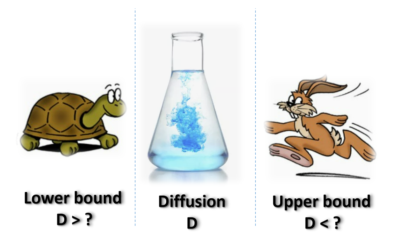
Figure 1: Given an arbitrary diffusive process and its related diffusion constant $D$, does $D$ obey any universal lower/upper bounds and in terms of which physical quantities? This is the question we address in this note.

Taking a similar perspective, one could ask whether the diffusion constants are also bounded from above or they can grow indefinitely (see cartoon in Fig.1). It turns out that causality, and in particular the requirement of avoiding superluminal propagation, imposes a strong upper bound on diffusion which takes the form Hartman:2017hhp :

$$D_{i}\,\leq\,v^{2}_{\text{lightcone}}\,\tau_{eq},$$ (6)

where $v_{\text{lightcone}}$ is the velocity, setting the causal lightcone in the theory, and $\tau_{eq}$ the equilibration time at which the system thermalizes, and after which hydrodynamics starts to apply. The equilibration time can be universally defined using the imaginary part of the first damped, and therefore non-hydrodynamic, mode as:

$$\tau^{-1}_{eq}\,\equiv\,\omega_{eq}=|\mathrm{Im}\,\omega_{1}|,$$ (7)

where $\omega_{1}$ is the frequency of the lowest of those modes.

Contrary to the equilibration time, the definition of the lightcone velocity related to the causal structure is far from trivial in systems which do not enjoy relativistic invariance and/or systems with emergent IR lightcone structures. In relativistic systems, the lightcone velocity is obviously set by the speed of light $c$. One simple example is given by Israel-Stewart relativistic hydrodynamics ISRAEL1979341 . There, the lightcone speed is immediately identified with the speed of light $c$ and the equilibration time with the IR relaxation time $\tau_{\pi}$ which is pheomenologically introduced in the framework. Indeed, within the Israel-Stewart formalism, the absence of superluminality can be re-written exactly as an upper bound on the shear diffusion constant $D_{\text{shear}}<c^{2}\tau_{\pi}$ Hartman:2017hhp ; Baggioli:2020ljz .

A first check of the upper bound in Eq.(6) was performed in Ref.Baggioli:2020ljz using different velocity scales. A more formal derivation, based on technical mathematical properties of the hydrodynamic perturbative expansion, was discussed in Grozdanov:2020koi . Interestingly, if one considers the momentum diffusion constant, instead of the $\eta/s$ ratio, all the known violations related to the breaking of spacetime symmetries disappear Baggioli:2020ljz .

Given the important role of hydrodynamics, recently, Ref.Arean:2020eus proposed to connect the lightcone velocity with the equilibration velocity. In particular, Ref.Arean:2020eus proposed a new bound which takes the following form:

$$D_{i}\,\leq\,v^{2}_{i,eq}\,\tau_{eq}\,.$$ (8)

Here, $v_{i,eq}$ is the equilibration velocity for the $i^{th}$ diffusive mode, defined as:

$$v_{eq}\,\equiv\,\frac{\omega_{eq}}{k_{eq}}\,.$$ (9)

where, to avoid clutter, the $i$ index has been dropped.
This idea uses the recent definition of the radius of convergence of hydrodynamics presented in PhysRevLett.122.251601 ; Grozdanov2019 ; Withers:2018srf and discussed further in Abbasi:2020ykq ; Jansen:2020hfd ; Baggioli:2020loj . In particular, the pair $(\omega_{eq},k_{eq})$ corresponds to the location of the first (closest to the origin) critical point of the hydrodynamic perturbative series. This point coincides with the collision (in general in the complex plane) between a first (in this case diffusive) hydrodynamic mode and a nearby non-hydrodynamic mode (or a tower of them), and it determines the radius of convergence of the hydrodynamic series. More precisely, we utilize the following definitions:

$$k_{eq}\,\equiv\,|k^{*}|\,,\qquad\omega_{eq}\,\equiv\,|\omega^{*}|\,,$$ (10)

where $(\omega^{*},k^{*})$ is the first critical point – the position of the collision for complex frequency and momentum, $k^{*},\omega^{*}\in\mathbb{C}$. In simple words, such a point determines the scale at which considering only conserved quantities is not enough anymore and the hydrodynamics description must be improved.

Few comments are in order. (I) The definition of the equilibration velocity is specific to the diffusive process considered. In this sense, it is quite a stretch to consider the bound in Eq.(8) as universal. Notice for example the crucial difference with the butterfly velocity proposal in Eq.(5), in which the velocity scale on the r.h.s. is the same for all the diffusion constants considered. (II) It is not clear how the bound in Eq.(8) connects with that in Eq.(6). In particular, Eq.(8) does not follow from the requirement of causality and furthermore $v_{eq}$ does not define nor the lightcone velocity nor the causal structure of any propagating process. (III) The equal sign in Eq.(8) follows trivially from assuming that the diffusive dispersion relation:

$$\omega\,=\,-i\,D\,k^{2}$$ (11)

is valid until the critical point $(\omega^{*},k^{*})$.
In particular simple algebra gives

$$\omega_{eq}\,=\,\,D\,k_{eq}^{2}\,\rightarrow\,1\,=\,\,D\,\frac{\omega_{eq}}{v_{eq}^{2}}\,\rightarrow\,D=v_{eq}^{2}\tau_{eq}\,.$$ (12)

That said, the observation of Arean:2020eus is interesting and it boils down to understand the following questions:

• Are there situations where the corrections to the hydrodynamic dispersion relation can be neglected until the critical point determining the radius of convergence of linearized hydrodynamics?

• Which conditions ensure the existence of such a scenarios and what is their meaning?

In this note, we consider the proposal of Ref.Arean:2020eus in homogeneous holographic models with long-range order, i.e. with spontaneously broken translational invariance. These systems display an $\text{AdS}_{2}$ IR near-horizon geometry and a peculiar new diffusive mode labelled crystal diffusion Donos:2019txg ; Baggioli:2020nay ; Baggioli:2020haa . In these holographic models, the lower bound Eq.(5) for crystal diffusion has already been verified in Baggioli:2020ljz . Our task now is to determine whether the inequivalence in Eq.(8) applies also to the same mode and which are the scales involved. Moreover, we analyze the connections and interplay between the lower bound on diffusion dictated by quantum chaos and this new upper bound determined by the breakdown of the hydrodynamic perturbative expansion. Finally, we provide some comments and thoughts for the future.

2 The holographic model

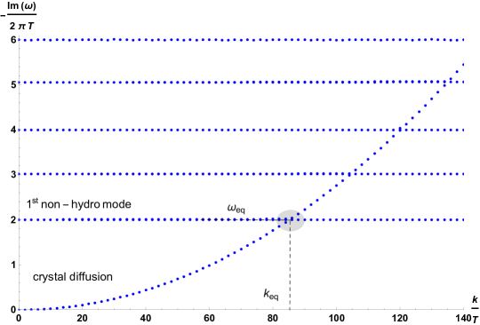
Figure 2: The longitudinal spectrum of quasinormal modes for $N=3$ and $m/T=500$. For simplicity, the attenuation constant of the longitudinal sound modes has been manually removed. The gray region emphasizes the location of the collision between the crystal diffusion mode and the first non-hydrodynamic $\text{AdS}_{2}$ mode, from which the parameters $\omega_{eq},k_{eq}$ are extracted as shown by the dashed lines. The tower of non-hydrodynamic modes follow the expected trend $\omega_{n}=2\pi T(n+\Delta)$, where in this case $\Delta=2$. Similar pictures can be obtained for different values $N$ and of $m/T$.

We consider a large class of holographic axion models Baggioli:2021xuv introduced and discussed in Baggioli:2014roa ; Alberte:2015isw ; Baggioli:2016rdj ; Baggioli:2019rrs and defined as follows:

$$S\,=\,\int d^{4}x\sqrt{-g}\left[\frac{R}{2}+3-\,m^{2}\,V(X)\right]\,,$$ (13)

where $X\equiv\frac{1}{2}\,g^{\mu\nu}\,\partial_{\mu}\phi^{I}\partial_{\nu}\phi^{I}$ and we have set the AdS radius to be unit. We choose an isotropic profile for the axion fields given by

$$\phi^{I}\,=\,x^{I}\,,$$ (14)

which represents a trivial solution of the equations of motion because of the global shift symmetry $\phi^{I}\rightarrow\phi^{I}+b^{I}$ of the action (13). The background geometry in Eddington-Filkenstein coordinates is written as:

$$ds^{2}=\frac{1}{u^{2}}\left[-f(u)\,dt^{2}-2\,dt\,du+dx^{2}+dy^{2}\right]\,,$$ (15)

where $u\in[0,u_{h}]$ is the radial holographic direction going from the boundary $u=0$ to the horizon, $f(u_{h})=0$. Finally, we have:

$$f(u)=u^{3}\int_{u}^{u_{h}}dv\;\left[\frac{3}{v^{4}}-\frac{m^{2}\,V(v^{2})}{v^{4}}\right]\,,$$ (16)

and consequently the temperature $T$ is defined as

$$T=-\frac{f^{\prime}(u_{h})}{4\pi}=\frac{6-2m^{2}\,V\left(u_{h}^{2}\right)}{8\pi\,u_{h}}\,,$$ (17)

while the entropy density is given by $s=2\pi/u_{h}^{2}$.

In the rest of the note, we will focus on the monomial form:

$$V(X)\,=\,X^{N}\,.$$ (18)

We refer to the previous literature Alberte:2017cch ; Alberte:2017oqx ; Baggioli:2018vfc ; Andrade:2019zey ; Ammon:2019wci ; Ammon:2019apj ; Baggioli:2019abx ; Ammon:2020xyv for more details concerning these models and their properties.
In these holographic models, the UV expansion of the $\phi^{I}$ bulk fields reads:

$$\phi^{I}(t,x,u)\,=\,\phi_{(0)}^{I}(t,x)\,+\,\phi_{(1)}^{I}(t,x)\,u^{5-2N}\,+\,\dots$$ (19)

Assuming standard quantization, one could verifiy that for $N<5/2$ the background solution $\phi^{I}=x^{I}$ plays the role of an external source, while for $N>5/2$ it describes a finite expectation value for the operators $\mathcal{O}^{I}$, dual to the axion fields. Following this argument, the breaking of translations is explicit for $N<5/2$ and spontaneous for $N>5/2$. In this note, we will only consider the case $N>5/2$.

3 Results

The longitudinal spectrum of systems with spontaneously broken translations features a peculiar mode with diffusive dispersion relation which is usually labelled “crystal diffusion”. Using the correct hydrodynamic description Armas:2019sbe , the diffusion constant of such a mode reads:

$$D\,=\,\xi\,\frac{\left(B+G-\mathcal{P}\right)\,\chi_{\pi\pi}}{s^{\prime}\,T^{2}\,v_{L}^{2}}\,.$$ (20)

The various parameters appearing in the equation above are: the Goldstones diffusion constant $\xi$, the bulk modulus $B$, the shear modulus $G$, the momentum susceptibility $\chi_{\pi\pi}$, the temperature derivative of the entropy $s^{\prime}$ and finally the so called crystal pressure $\mathcal{P}$. The hydrodynamic formula Eq.(20) has been successfully matched to the holographic results Ammon:2020xyv ; Baggioli:2019abx after some initial, and then resolved, tension Ammon:2019apj .

The dispersion relation of the crystal diffusion mode is shown in Fig.2 for very low values of temperature. The characteristic quadratic scaling and the corresponding slope are consistent with the previous theoretical computations. In Fig.2, the lowest non-hydrodynamic modes $\omega=-i\,\omega_{n}$ are shown as well. As explained in the previous literature Faulkner:2009wj ; Edalati:2010hk and discussed in Arean:2020eus , these modes have a quite flat dispersion relation at low temperatures and they appear equally separated. In particular, this tower of non-hydrodynamic modes belongs to the IR $\text{AdS}_{2}$ spectrum and it is given by:

$$\omega_{n}\,=\,2\,\pi\,T\,\left(\Delta_{0}\,+\,n\right)\qquad\text{for}\qquad T\rightarrow 0\,,$$ (21)

where $n$ is the index labelling the modes and the constant $\Delta_{0}$ corresponds to the conformal dimension of the lowest operator in the $\text{AdS}_{2}$ IR fixed point evaluated at zero momentum, $\Delta_{0}=\Delta(k=0)$Arean:2020eus .
Given the presence of these modes, we can immediately identify the value of the lowest ($n=0$) frequency in Eq.(21) with the equilibration timescale:

$$\omega_{eq}=\tau^{-1}_{eq}=\omega_{0}=2\pi\,\Delta_{0}\,T\,.$$ (22)

We plot the value of the normalized equilibration frequency in function of $m/T$ at low temperatures in Fig.3. The curves approach nicely a common asymptotic $T=0$ value which is given by $\Delta_{0}=2$. Importantly, this value is completely independent of the choice of the potential and in particular the value of the power $N$ .

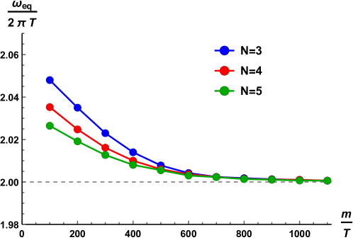
Figure 3: The equilibration frequency $\omega_{eq}$ in function of the dimensionless temperature for various $N=3,4,5$. All the curves approach asymptotically a constant value given by $\Delta_{0}=2$.

Let us now move to discuss the interplay between the diffusive hydrodynamic mode and the first non-hydro mode. We have zoomed in the area in which the crystal diffusion mode and the first non-hydrodynamic mode approach each other, which is indicated with a gray shaded region in Fig.2. The results are more clearly shown in Fig.4. From there, it is evident that the two modes display an avoided crossing dynamics as noticed already in Arean:2020eus . In particular, we numerically observe (see Arean:2020eus for an analytic proof) that the avoided crossing mechanism becomes more and more evident by increasing the temperature. This is consistent with the observation that the collision between the diffusive mode and the first non-hydrodynamic mode happens for complex momentum, but the imaginary part of the critical point tends to zero with the temperature $T$. Therefore, at low temperature, we can approximate the equilibration scale with the real value of the critical momentum:

$$k_{eq}\,\equiv\,|k^{*}|\,\approx\mathrm{Re}\,k^{*}$$ (23)

which, together with the critical frequency $\omega^{*}$, is easily readable from the dispersion relation of the modes in the longitudinal spectrum, as shown in Fig.2.

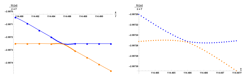
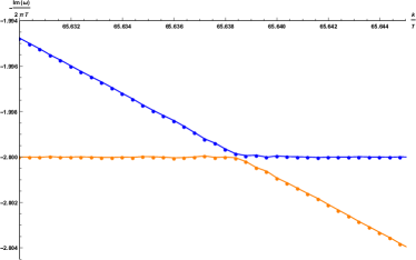
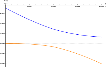
Figure 4: Top Left: The ”almost” collision between the diffusive mode and the first non-hydrodynamic mode. Top Right: A zoom of the avoided crossing dynamics for $N=3$ and $m/T=900$. The gap between the two modes becomes smaller and smaller going to lower temperature. Bottom panels: The same figures at larger temperature, $m/T=300$. Here, the avoided crossing is more pronounced and the separation between the two curves is larger. This implies that the imaginary part of the critical complex momentum is larger.

In summary, we can extract both parameters, $\omega_{eq},k_{eq}$, simply by looking at the dispersion relations of the two lowest modes as shown in Figures 2 and 4. At this point, we can also straightforwardly define the equilibration velocity as:

$$v_{eq}\,\equiv\,\frac{\omega_{eq}}{k_{eq}}\,.$$ (24)

We show the behaviour of the non-normalized equilibration velocity in function of temperature in the left panel of Fig.5. Interestingly, we observed a very clear $T^{1/2}$ scaling close to zero temperature. Given that $\omega_{eq}\sim T$ at low temperature (Eq.(21)), we can derive that in such a regime the radius of convergence of hydrodynamics goes as:

$$k_{eq}\,\sim\,T^{1/2}\,.$$ (25)

This is consistent with the idea that the convergence properties of hydrodynamics become worse and worse upon lowering the temperature Baggioli:2020loj . In other words, hydrodynamics breaks down at larger distances going towards zero temperature. Eq.(25) is also consistent with previous results for charged holographic backgrounds and realistic liquids Abbasi:2020ykq ; Jansen:2020hfd ; Baggioli:2020loj .

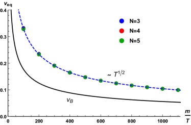
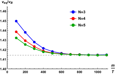
Figure 5: Left: The behaviour of the equilibration velocity in function of the dimensionless temperature $m/T$ for various values of $N=3,4,5$. The dashed line shows the $T^{1/2}$ scaling. Right: The comparison with the butterfly velocity. At low temperatures, the ratio of the two velocities approach a constant value, $\sqrt{\Delta_{0}}=\sqrt{2}$.

At this stage, we want to compare the behaviour of the equilibration velocity with that of the butterfly velocity, which has a fundamental role in the diffusion bounds discussed in the introduction. The butterfly velocity can be obtained from horizon data and in our background is given by:

$$v_{B}^{2}\,=\,\frac{\pi\,T}{u_{h}}\,.$$ (26)

In the limit of $m/T\rightarrow\infty$, the radius of the horizon goes to a constant and therefore we obtain the expected scaling $v_{B}\sim T^{1/2}$. Interestingly, the ratio between the two velocity scales approaches a constant, given by $\sqrt{\Delta_{0}}$, in the low temperature limit. We notice that for canonically normalized operators with unitary conformal dimension in the $AdS_{2}$ IR fixed point, the two velocities would exactly coincide at low temperature. More in general, we find that:

$$v_{eq}\,>\,v_{B}\,.$$ (27)

If one considers the butterfly velocity as an emergent lightcone speed of some (non-relativistic) quantum chaotic system, the relation just obtained looks quite dangerous since it would imply a superluminal propagation with speed $v_{eq}$ outside of the causal lightcone. Nevertheless, the equilibration velocity $v_{eq}$ does not correspond to any propagating modes. In other words, in these cases, there is absolutely no excitation propagating at such speed. In any case, this relation looks certainly interesting and it deserves further understanding. It also implies that the thermalization speed, defined as in Eq.(24), is faster than the speed of information scrambling. It would be important to understand how universal this hierarchy is and which are the physical consequences.

Another indication that the equilibration speed $v_{eq}$ cannot play the role of the lightcone velocity in the bound of Hartman:2017hhp is given by the fact that in this model the longitudinal speed of sound is much larger than the equilibration velocity. In this sense, if one had to choose a lightcone velocity, the sound speed would be the most appropriate.

After having identified all the scales entering in the bound of Eq.(8), we can finally test its validity for the crystal diffusion mode. In Fig.6, we plot the dimensionless ratio $D/v_{eq}^{2}\tau_{eq}$ in function of the dimensionless inverse temperature $m/T$ at small temperatures and for various potentials, $N=3,4,5$. In all the cases, we notice that this ratio approaches unity at $T\rightarrow 0$ confirming the validity of the relationship:

$$D\,=\,v_{eq}^{2}\tau_{eq}\qquad\text{for}\qquad T\rightarrow 0\,.$$ (28)

Moreover, we obtain that in general

$$D\,\leq\,v_{eq}^{2}\tau_{eq}$$ (29)

and that therefore the bound Eq.(8) proposed in Arean:2020eus indeed holds. This constitutes an explicit confirmation that even for the crystal diffusion mode, the diffusion constant is bounded from above by the equilibration scales $v_{eq}$ and $\tau_{eq}$.

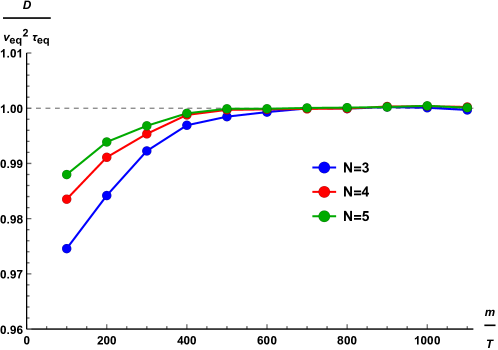
Figure 6: The dimensionless ratio $D/(v_{eq}^{2}\tau_{eq})$ in function of the inverse dimensionless temperature for various powers $N=3,4,5$. All the curves approach the unit value at low temperature. Moreover, all curves are consistent with the inequality $D\leq v_{eq}^{2}\tau_{eq}$.

4 Conclusions

In summary, in this short note, we have confirmed the validity of the diffusion bound defined in terms of the hydrodynamics breakdown data proposed in Ref.Arean:2020eus for the crystal diffusion mode present in all holographic systems with spontaneously broken translations. Importantly, in our case, the collision determining the equilibration scales happens for real values of the momentum $k$ and therefore it is easily extracted from the dispersion relation of the lowest quasinormal modes.

Moreover, we do find that, for arbitrary values of the temperature, the diffusion constant is confined in an range determined by:

$$v_{B}^{2}\,\tau_{L}\,\leq\,D\,\leq\,v_{eq}^{2}\,\tau_{eq},$$ (30)

which is shown in Fig.7. Importantly, approaching the zero temperature limit this allowed region shrinks and at exactly zero temperature the two limits collapse on each other. This means that the universal bounds determine uniquely the value of the diffusion constant at zero temperature:

$$\left(v_{B}^{2}\,\tau_{L}\right)|_{T=0}\,=\,D|_{T=0}\,=\,\left(v_{eq}^{2}\,\tau_{eq}\right)|_{T=0}\,.$$ (31)

This is a very interesting and new outcome whose universal character must be investigated further.

5 Additional comments

We conclude with several comments and ideas for the future.

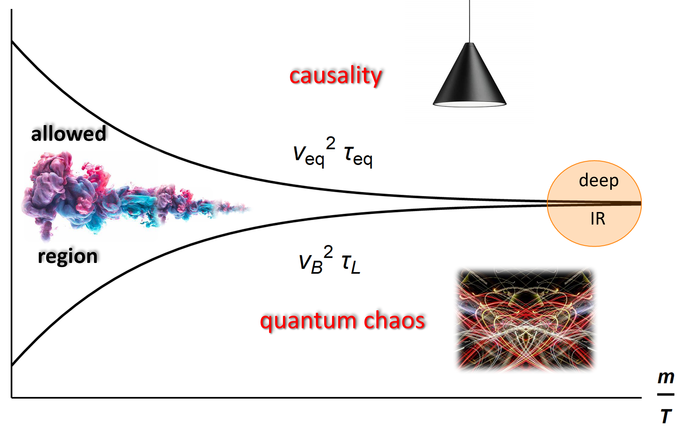
Figure 7: A cartoon of the allowed region for the diffusion constant $D$. The upper edge comes from the scales related to the breakdown of linearized hydrodynamics. While, the lower one is dictated by the data of quantum chaos Baggioli:2020ljz . Both curves merge in the limit of $T\rightarrow 0$.

• One interesting point is the connection between the diffusivity bound $D\leq v_{eq}^{2}\tau_{eq}$ and the higher order corrections to the diffusive dispersion relation. As we have shown in the main text, if the diffusive behaviour $\omega=-iDk^{2}$ persists until the collision point, the equality trivially holds. What happens if that is not the case? In general, the dispersion relation is given by a perturbative expansion in momentum of the type:

  $$\omega\,=\,-i\left(Dk^{2}+a_{1}\,k^{4}\,+\,a_{2}\,k^{6}+\dots\,\right),$$ (32)

  where for simplicity we have ignored any possible real part and considered a purely imaginary mode. Let us consider that, upon reaching the critical point $(\omega^{*},k^{*})$, the first higher order correction cannot be neglected. Then, we have:

  $$\omega_{eq}\,=\,Dk_{eq}^{2}+a_{1}\,k_{eq}^{4}$$ (33)

  which, after some manipulations, gives:

  $$D\,=\,v_{eq}^{2}\tau_{eq}\,-\,\frac{a_{1}}{v_{eq}^{2}\,\tau_{eq}}\,.$$ (34)

  The extension to higher order terms is trivial and for simplicity not shown here. By looking at Eq.(34), one can infer that the validity of the upper diffusion bound depends crucially on the signs of the higher order corrections. In particular, the higher order terms in the diffusive dispersion relations introduce corrections of order $\mathcal{O}(1/v_{eq}^{2n}\tau_{eq}^{n})$, controlled by the various new coefficients $a_{n}$. Is there any physical requirement (e.g. causality) that fixes the sign of these coefficients and therefore the validity of the upper bound? That seems indeed the case. The univalence property of the hydrodynamics expansion put stringent bounds on all the higher order coefficients Grozdanov:2020koi . For example, it constraints the first of them, labelled $a_{1}$ above, to be positive. In other words, it is very tempting to claim that the validity of the upper bound proposed in Arean:2020eus can be formally derived using mathematical properties of the hydrodynamic series Grozdanov:2020koi . A simple scenario where this mechanism appears is the telegrapher equation BAGGIOLI2020 :

  $$\omega^{2}+i\omega/\tau\,=\,v^{2}\,k^{2}\,.$$ (35)

  In this case, the purely diffusive dispersion law gets corrected before the poles collision as:

  $$\omega\,=\,-\,i\,D\,k^{2}\,-\,i\,v^{4}\,\tau^{3}\,k^{4}\,+\,\dots$$ (36)

  and the corresponding higher order coefficient reads $a_{1}=v^{4}\,\tau^{3}$. Stability, and more precisely the requirement of having $\tau>0$ (a relaxation process and not an “exploding” one), implies that $a_{1}>0$ and therefore that the diffusion constant is bounded from above, as discussed in the previous paragraph.

• It would be interesting to understand better the zero temperature relation in Eq.(31). To the best of our knowledge, the collapse of the two bounds at zero temperature has not been observed nor discussed before. How universal is this feature? What can we learn from it? Is it possible to maintain a finite range of allowed values at zero temperature or the two bounds always collapse?

• In all this discussion, the value of the constant $\Delta_{0}$ plays a fundamental role. In particular, the concrete value $\sqrt{\Delta_{0}}$ controls the ratio between the equilibration velocity and the butterfly velocity at low temperature. It would be interesting to understand if any physical requirement (e.g. unitarity and the corresponding bounds on the conformal dimensions) constraints $\Delta_{0}>1$ and if not what is the meaning of this role-reversal phenomenon.

• A priori, it is not clear what is the relation between the equilibration velocity $v_{eq}$ and the causal structure of the system. In particular, such a velocity in general does not correspond to any propagating mode. Interestingly, taking the telegrapher equation (35), one can derive that the equilibration velocity $v_{eq}$ coincides exactly with the sound speed of the emergent propagating mode at large momentum. In this simplified scenario, it does corresponding to a propagating mode at short distance.

• In the main text, we have derived that in the low temperature limit, $\tau_{eq}^{-1}=2\pi\,\Delta_{0}\,T$. This relaxation time has the same temperature dependence of the Planckian time and the Liapunov time but with a different numerical prefactor. In particular we have:

  $$(\tau_{pl},\tau_{L},\tau_{eq})\,T\,=\,\left(1,\frac{1}{2\pi},\frac{1}{2\pi\,\Delta_{0}}\right)\,.$$ (37)

  Moreover, the hierarchy of these timescales depends crucially on the value of $\Delta_{0}$. Also, the situation might be substantially different away from maximal chaos Choi:2020tdj where the Maldacena bound Maldacena:2015waa is not saturated and $\tau_{L}>\frac{1}{2\pi\,T}$. Which is the order of these timescales and how can it be changed?

• In Arean:2020eus , the equilibration velocity has been defined using the critical point which determines the breakdown of the hydrodynamics expansion and in particular of the diffusive dispersion relation. In principle, there are other points in the complex plane which assume a particular role – the pole-skipping points Grozdanov:2017ajz ; Blake:2018leo ; Blake:2017ris ; Ahn:2020baf . Given a certain Green function, those are the points at which the zeros and the poles cross, rendering the Green function indeterminate. Following Arean:2020eus , one could define a pole-skipping velocity:

  $$v^{\mathcal{O}}_{skip}\,\equiv\,\frac{|\omega_{skip}|}{|k_{skip}|},$$ (38)

  where $(\omega_{skip},k_{skip})$ indicates the location of the first pole skipping point in the complex plane and the index $\mathcal{O}$ the operator whose Green function is considered. Notice that if one considers the energy-energy correlator, one finds $v^{\epsilon}_{skip}=v_{B}$ and $\omega_{skip}=\tau_{L}^{-1}$ Grozdanov:2017ajz . In this sense, for the energy correlator, we have the following identification:

  $$\frac{v^{2}_{skip}}{\omega_{skip}}\,=\,v_{B}^{2}\,\tau_{L}$$ (39)

  and therefore one can immediately write down a lower bound of the type:

  $$D_{\epsilon}\,\geq\,\frac{v^{2}_{skip}}{\omega_{skip}}\,.$$ (40)

  The question whether a more general bound:

  $$D_{\mathcal{O}}\,\geq\,\frac{v^{2}_{\mathcal{O},skip}}{\omega_{\mathcal{O},skip}}\,$$ (41)

  exists for an arbitrary operator $\mathcal{O}$ is valuable and it can be easily investigated with the existing techniques. Preliminary indications private seem to suggest our hypothesis.

• As already mentioned, the speed of longitudinal sound $v_{L}$ in this model is much larger than the equilibration speed $v_{eq}$. This implies that (I) the equilibration velocity cannot be taken as the one determining the causal lightcone and (II) that the bound $D\leq v_{eq}^{2}\tau_{eq}$ is more stringent than the one coming from causality as in Hartman:2017hhp .

• Finally, it would be interesting to consider IR fixed point with dangerously irrelevant deformations Davison:2018ofp . There, the equilibration time is expected to be parametrically longer, $\tau_{eq}\gg T^{-1}$, and the full picture could change substantially. Hyperscaling-Lifshitz IR geometries are also a straightforward generalization of this program.

The emerging global picture suggests intriguing and possibly fundamental connections between transport, quantum chaos, hydrodynamics and pole skipping which are left to be revealed.

We plan to come back to some of these questions in the near future.

Acknowledgments

We thank Sebastian Grieninger for providing the numerical codes used in previous works and for useful comments. We thank Saso Grozdanov, Keun-Young Kim, Yongjun Ahn and Hyun-Sik Jeong for reading a preliminary version of the manuscript and providing useful comments and suggestions. We thank Keun-Young Kim, Yongjun Ahn, Hyun-Sik Jeong and Ya-Wen Sun for sharing with us unpublished results and for correcting a mistake contained in the previous version of this manuscript. N.W. and W.J.L. are supported by NSFC No.11905024 and No.DUT19LK20. M.B. acknowledges the support of the Shanghai Municipal Science and Technology Major Project (Grant No.2019SHZDZX01).

Appendix A Equations for the perturbations

We align the momentum $k$ along the $y$ direction. The perturbations in the longitudinal sector are given by

$$\{h_{x,\,{s}}=1/2\,(h_{xx}+h_{yy}),\,h_{x,\,{a}}=1/2\,(h_{xx}-h_{yy}),\,\delta\phi_{y},\,h_{tt},\,h_{ty}\}\,,$$ (42)

We use a radial gauge. The final set of equations for the perturbations reads

$$uf^{\prime}\,\delta\phi_{y}^{\prime}\,\dot{V}\,+2\,u^{2}\,f\,\delta\phi_{y}^{\prime}\,\ddot{V}+u\,f\,\delta\phi_{y}^{\prime\prime}\,\dot{V}-2\,f\,\delta\phi_{y}^{\prime}\,\dot{V}-k^{2}\,u\,\delta\phi_{y}\,\dot{V}-k^{2}\,u^{3}\,\delta\phi_{y}\,\ddot{V}$$

$$+i\,k\,u\,h_{x,\,{a}}\,\dot{V}-i\,k\,u^{3}\,h_{x,\,{s}}\,\ddot{V}+2\,i\,u^{2}\,\omega\,\delta\phi_{y}\,\ddot{V}+u\,h_{ty}^{\prime}\,\dot{V}+2\,i\,u\,\omega\,\delta\phi_{y}^{\prime}\,\dot{V}$$

$$-2\,i\,\omega\,\delta\phi_{y}\dot{V}-2\,h_{ty}\left(\dot{V}-u^{2}\,\ddot{V}\right)=0$$ (43)

$$u(f\left(uf^{\prime}\,h_{x,\,{s}}^{\prime}-2\,f\,h_{x,\,{s}}^{\prime}-2\,i\,k\,m^{2}\,u^{3}\,\delta\phi_{y}\,\ddot{V}-u\,h_{tt}^{\prime\prime}+4\,h_{tt}^{\prime}\right)$$

$$+k\,h_{ty}\left(i\,u\,f^{\prime}-2\,i\,f+2\,u\,\omega\right)+h_{x,\,{s}}\left(2\,m^{2}\,u^{3}\,f\,\ddot{V}+\omega\,\left(i\,u\,f^{\prime}-2\,i\,f+2\,u\,\omega\right)\right))$$

$$+h_{tt}\left(u\left(-uf^{\prime\prime}+4\,f^{\prime}+2\,m^{2}\,u\,\dot{V}\right)-12\,f+k^{2}\,u^{2}-2\,m^{2}\,V-2\,i\,u\,\omega+6\right)=0$$ (44)

$$2h_{ty}\left(u\left(f^{\prime}+m^{2}\,u\,\dot{V}\right)-3\,f-m^{2}\,V+3\right)$$

$$-u\left(u\,f\,h_{ty}^{\prime\prime}-2\,f\,h_{ty}^{\prime}+i\,k\,u\,h_{tt}^{\prime}+k\,u\,\omega\,h_{x,\,{s}}+k\,u\,\omega\,h_{x,\,{a}}-2\,i\,m^{2}\,u\,\omega\,\delta\phi_{y}\,\dot{V}+i\,u\,\omega\,h_{ty}^{\prime}\right)$$

$$+2\,i\,k\,u\,h_{tt}=0$$ (45)

$$h_{x,\,{s}}\left(2\,u\left(f^{\prime}+m^{2}\,u\,\dot{V}\right)-6\,f+k^{2}\,u^{2}-2\,m^{2}\,V+4\,i\,u\,\omega+6\right)-u^{2}\,f^{\prime}\,h_{x,\,{s}}^{\prime}$$

$$-u^{2}\,f^{\prime}\,h_{x,\,{a}}^{\prime}+2\,u\,h_{x,\,{a}}\,f^{\prime}-u^{2}\,f\,h_{x,\,{s}}^{\prime\prime}-u^{2}\,f\,h_{x,\,{a}}^{\prime\prime}+4\,u\,f\,h_{x,\,{s}}^{\prime}+2\,u\,f\,h_{x,\,{a}}^{\prime}-6\,f\,h_{x,\,{a}}$$

$$+k^{2}\,u^{2}\,h_{x,\,{a}}+2\,i\,k\,u\,h_{ty}+2\,m^{2}\,u^{2}\,h_{x,\,{a}}\,\dot{V}-2\,m^{2}\,h_{x,\,{a}}\,V-2\,i\,u^{2}\,\omega\,h_{x,\,{s}}^{\prime}$$

$$-2\,i\,u^{2}\,\omega\,h_{x,\,{a}}^{\prime}-2\,u\,h_{tt}^{\prime}+6h_{tt}(u)+2\,i\,u\,\omega\,h_{x,\,{a}}+6h_{x,\,{a}}=0$$ (46)

$$h_{x,\,{s}}\left(2\,u\left(f^{\prime}+m^{2}\,u\,\dot{V}\right)-6\,f+k^{2}\,u^{2}-2\,m^{2}\,V+4\,i\,u\,\omega+6\right)-u^{2}\,f^{\prime}\,h_{x,\,{s}}^{\prime}+u^{2}\,f^{\prime}\,h_{x,\,{a}}^{\prime}$$

$$-2\,u\,h_{x,\,{a}}\,f^{\prime}-u^{2}\,f\,h_{x,\,{s}}^{\prime\prime}+u^{2}\,f\,h_{x,\,{a}}^{\prime\prime}+4\,u\,f\,h_{x,\,{s}}^{\prime}-2\,u\,fh_{x,\,{a}}^{\prime}+6\,f\,h_{x,\,{a}}+k^{2}\,u^{2}\,h_{x,\,{a}}$$

$$-4\,i\,k\,m^{2}\,u^{2}\,\delta\phi_{y}\,\dot{V}-2\,i\,k\,u^{2}\,h_{ty}^{\prime}+6\,i\,k\,u\,h_{ty}-2\,m^{2}\,u^{2}\,h_{x,\,{a}}\,\dot{V}+2\,m^{2}\,h_{x,\,{a}}\,V$$

$$-2\,i\,u^{2}\,\omega\,h_{x,\,{s}}^{\prime}+2\,i\,u^{2}\,\omega\,h_{x,\,{a}}^{\prime}-2\,u\,h_{tt}^{\prime}+6\,h_{tt}-2\,i\,u\,\omega\,h_{x,\,{a}}-6\,h_{x,\,{a}}=0$$ (47)

$$-6\,h_{tt}+u\,(u\,f^{\prime}\,h_{x,\,{s}}^{\prime}-2\,f\,h_{x,\,{s}}^{\prime}-2\,i\,k\,m^{2}\,u^{3}\,\delta\phi_{y}\,\ddot{V}+i\,k\,u\,h_{ty}^{\prime}-2\,i\,k\,h_{ty}$$

$$+2\,m^{2}\,u^{3}\,h_{x,\,{s}}\,\ddot{V}-u\,h_{tt}^{\prime\prime}+4\,h_{tt}^{\prime}+2\,i\,u\,\omega\,h_{x,\,{s}}^{\prime}-2\,i\,\omega\,h_{x,\,{s}})=0$$ (48)

$$k\,u\left(h_{x,\,{s}}^{\prime}+h_{x,\,{a}}^{\prime}\right)-i\,u\,\left(2\,m^{2}\,\delta\phi_{y}^{\prime}\,\dot{V}+h_{ty}^{\prime\prime}\right)+2\,i\,h_{ty}^{\prime}=0$$ (49)

$$h_{x,\,{s}}^{\prime\prime}=0,$$ (50)

where the following notations $\dot{V}\equiv dV(X)/dX,\,\ddot{V}\equiv d^{2}V(X)/dX^{2}$ are used.
The quasinormal modes are obtained using pseudo-spectral methods. For more details about the numerical procedure see Grieninger:2020wsb .

References

- (1) L. Landau and E. Lifshitz, Fluid Mechanics: Volume 6. No. v. 6. Elsevier Science, 2013.
- (2) P. C. Martin, O. Parodi and P. S. Pershan, Unified hydrodynamic theory for crystals, liquid crystals, and normal fluids, Phys. Rev. A 6 (Dec, 1972) 2401–2420.
- (3) G. Policastro, D. T. Son and A. O. Starinets, The Shear viscosity of strongly coupled N=4 supersymmetric Yang-Mills plasma, Phys. Rev. Lett. 87 (2001) 081601, [hep-th/0104066].
- (4) S. S. Gubser, I. R. Klebanov and A. A. Tseytlin, String theory and classical absorption by three-branes, Nucl. Phys. B 499 (1997) 217–240, [hep-th/9703040].
- (5) I. R. Klebanov, World volume approach to absorption by nondilatonic branes, Nucl. Phys. B 496 (1997) 231–242, [hep-th/9702076].
- (6) P. Kovtun, Lectures on hydrodynamic fluctuations in relativistic theories, J. Phys. A 45 (2012) 473001, [1205.5040].
- (7) J. Zaanen, Why the temperature is high, Nature 430 (Jul, 2004) 512–513.
- (8) J. Zaanen, Planckian dissipation, minimal viscosity and the transport in cuprate strange metals, SciPost Phys. 6 (2019) 61.
- (9) J. A. N. Bruin, H. Sakai, R. S. Perry and A. P. Mackenzie, Similarity of scattering rates in metals showing t-linear resistivity, Science 339 (2013) 804–807.
- (10) K. Behnia and A. Kapitulnik, A lower bound to the thermal diffusivity of insulators, Journal of Physics: Condensed Matter 31 (jul, 2019) 405702.
- (11) S. Sachdev, Bekenstein-hawking entropy and strange metals, Phys. Rev. X 5 (Nov, 2015) 041025.
- (12) A. A. Patel and S. Sachdev, Theory of a planckian metal, Phys. Rev. Lett. 123 (Aug, 2019) 066601.
- (13) J. Maldacena, S. H. Shenker and D. Stanford, A bound on chaos, JHEP 08 (2016) 106, [1503.01409].
- (14) C. H. Mousatov and S. A. Hartnoll, On the planckian bound for heat diffusion in insulators, Nature Physics (Mar, 2020) .
- (15) Y. Cao, D. Chowdhury, D. Rodan-Legrain, O. Rubies-Bigorda, K. Watanabe, T. Taniguchi et al., Strange metal in magic-angle graphene with near planckian dissipation, Phys. Rev. Lett. 124 (Feb, 2020) 076801.
- (16) V. Martelli, J. L. Jiménez, M. Continentino, E. Baggio-Saitovitch and K. Behnia, Thermal transport and phonon hydrodynamics in strontium titanate, Phys. Rev. Lett. 120 (Mar, 2018) 125901.
- (17) J. Zhang, E. D. Kountz, K. Behnia and A. Kapitulnik, Thermalization and possible signatures of quantum chaos in complex crystalline materials, Proceedings of the National Academy of Sciences 116 (2019) 19869–19874, [https://www.pnas.org/content/116/40/19869.full.pdf].
- (18) A. Lucas, Operator size at finite temperature and Planckian bounds on quantum dynamics, Phys. Rev. Lett. 122 (2019) 216601, [1809.07769].
- (19) T. Hartman, S. A. Hartnoll and R. Mahajan, Upper Bound on Diffusivity, Phys. Rev. Lett. 119 (2017) 141601, [1706.00019].
- (20) T. Schafer and D. Teaney, Nearly Perfect Fluidity: From Cold Atomic Gases to Hot Quark Gluon Plasmas, Rept. Prog. Phys. 72 (2009) 126001, [0904.3107].
- (21) S. Cremonini, The Shear Viscosity to Entropy Ratio: A Status Report, Mod. Phys. Lett. B25 (2011) 1867–1888, [1108.0677].
- (22) M. Luzum and P. Romatschke, Conformal Relativistic Viscous Hydrodynamics: Applications to RHIC results at s(NN)**(1/2) = 200-GeV, Phys. Rev. C 78 (2008) 034915, [0804.4015].
- (23) J. L. Nagle, I. G. Bearden and W. A. Zajc, Quark-Gluon Plasma at RHIC and the LHC: Perfect Fluid too Perfect?, New J. Phys. 13 (2011) 075004, [1102.0680].
- (24) C. Shen, U. Heinz, P. Huovinen and H. Song, Radial and elliptic flow in Pb+Pb collisions at the Large Hadron Collider from viscous hydrodynamic, Phys. Rev. C 84 (2011) 044903, [1105.3226].
- (25) J. Erdmenger, P. Kerner and H. Zeller, Non-universal shear viscosity from einstein gravity, Physics Letters B 699 (2011) 301 – 304.
- (26) L. Alberte, M. Baggioli and O. Pujolas, Viscosity bound violation in holographic solids and the viscoelastic response, JHEP 07 (2016) 074, [1601.03384].
- (27) S. A. Hartnoll, D. M. Ramirez and J. E. Santos, Entropy production, viscosity bounds and bumpy black holes, JHEP 03 (2016) 170, [1601.02757].
- (28) P. Burikham and N. Poovuttikul, Shear viscosity in holography and effective theory of transport without translational symmetry, Phys. Rev. D94 (2016) 106001, [1601.04624].
- (29) A. Rebhan and D. Steineder, Violation of the Holographic Viscosity Bound in a Strongly Coupled Anisotropic Plasma, Phys. Rev. Lett. 108 (2012) 021601, [1110.6825].
- (30) X.-H. Ge, S.-K. Jian, Y.-L. Wang, Z.-Y. Xian and H. Yao, Violation of the viscosity/entropy bound in translationally invariant non-Fermi liquids, 1810.00669.
- (31) M. P. Gochan, H. Li and K. S. Bedell, Viscosity Bound Violation in Viscoelastic Fermi Liquids, 1801.08627.
- (32) J. P. Figueroa and K. Pallikaris, Quartic Horndeski, planar black holes, holographic aspects and universal bounds, JHEP 20 (2020) 090, [2006.00967].
- (33) T. D. Cohen, Is there a “most perfect fluid” consistent with quantum field theory?, Phys. Rev. Lett. 99 (Jul, 2007) 021602.
- (34) M. Baggioli and W.-J. Li, Universal Bounds on Transport in Holographic Systems with Broken Translations, SciPost Phys. 9 (2020) 007, [2005.06482].
- (35) K. Trachenko and V. V. Brazhkin, Minimal quantum viscosity from fundamental physical constants, Science Advances 6 (2020) .
- (36) K. Trachenko, V. Brazhkin and M. Baggioli, Similarity between the kinematic viscosity of quark-gluon plasma and liquids at the viscosity minimum, 2003.13506.
- (37) K. Trachenko, M. Baggioli, K. Behnia and V. V. Brazhkin, Universal lower bounds on energy and momentum diffusion in liquids, Phys. Rev. B 103 (2021) 014311, [2009.01628].
- (38) S. A. Hartnoll, Theory of universal incoherent metallic transport, Nature Phys. 11 (2015) 54, [1405.3651].
- (39) M. Blake, Universal Charge Diffusion and the Butterfly Effect in Holographic Theories, Phys. Rev. Lett. 117 (2016) 091601, [1603.08510].
- (40) M. Blake, Universal Diffusion in Incoherent Black Holes, Phys. Rev. D94 (2016) 086014, [1604.01754].
- (41) A. I. Larkin and Y. N. Ovchinnikov, Quasiclassical Method in the Theory of Superconductivity, Soviet Journal of Experimental and Theoretical Physics 28 (June, 1969) 1200.
- (42) R. A. Davison, S. A. Gentle and B. Gouteraux, Slow relaxation and diffusion in holographic quantum critical phases, Phys. Rev. Lett. 123 (2019) 141601, [1808.05659].
- (43) Y. Gu, A. Lucas and X.-L. Qi, Spread of entanglement in a Sachdev-Ye-Kitaev chain, JHEP 09 (2017) 120, [1708.00871].
- (44) Y. Ling and Z.-Y. Xian, Holographic Butterfly Effect and Diffusion in Quantum Critical Region, JHEP 09 (2017) 003, [1707.02843].
- (45) Y. Gu, A. Lucas and X.-L. Qi, Energy diffusion and the butterfly effect in inhomogeneous Sachdev-Ye-Kitaev chains, SciPost Phys. 2 (2017) 018, [1702.08462].
- (46) M. Blake and A. Donos, Diffusion and Chaos from near AdS2 horizons, JHEP 02 (2017) 013, [1611.09380].
- (47) M. Blake, R. A. Davison and S. Sachdev, Thermal diffusivity and chaos in metals without quasiparticles, Phys. Rev. D96 (2017) 106008, [1705.07896].
- (48) S.-F. Wu, B. Wang, X.-H. Ge and Y. Tian, Collective diffusion and quantum chaos in holography, Phys. Rev. D97 (2018) 106018, [1702.08803].
- (49) W. Li, S. Lin and J. Mei, Thermal diffusion and quantum chaos in neutral magnetized plasma, Phys. Rev. D100 (2019) 046012, [1905.07684].
- (50) X.-H. Ge, S.-J. Sin, Y. Tian, S.-F. Wu and S.-Y. Wu, Charged BTZ-like black hole solutions and the diffusivity-butterfly velocity relation, JHEP 01 (2018) 068, [1712.00705].
- (51) W.-J. Li, P. Liu and J.-P. Wu, Weyl corrections to diffusion and chaos in holography, JHEP 04 (2018) 115, [1710.07896].
- (52) H.-S. Jeong, Y. Ahn, D. Ahn, C. Niu, W.-J. Li and K.-Y. Kim, Thermal diffusivity and butterfly velocity in anisotropic Q-Lattice models, JHEP 01 (2018) 140, [1708.08822].
- (53) M. Baggioli and W.-J. Li, Diffusivities bounds and chaos in holographic Horndeski theories, JHEP 07 (2017) 055, [1705.01766].
- (54) K.-Y. Kim and C. Niu, Diffusion and Butterfly Velocity at Finite Density, JHEP 06 (2017) 030, [1704.00947].
- (55) I. L. Aleiner, L. Faoro and L. B. Ioffe, Microscopic model of quantum butterfly effect: out-of-time-order correlators and traveling combustion waves, Annals Phys. 375 (2016) 378–406, [1609.01251].
- (56) A. A. Patel, D. Chowdhury, S. Sachdev and B. Swingle, Quantum butterfly effect in weakly interacting diffusive metals, Phys. Rev. X 7 (2017) 031047, [1703.07353].
- (57) A. A. Patel and S. Sachdev, Quantum chaos on a critical Fermi surface, Proc. Nat. Acad. Sci. 114 (2017) 1844–1849, [1611.00003].
- (58) A. Bohrdt, C. Mendl, M. Endres and M. Knap, Scrambling and thermalization in a diffusive quantum many-body system, New J. Phys. 19 (2017) 063001, [1612.02434].
- (59) Y. Werman, S. A. Kivelson and E. Berg, Quantum chaos in an electron-phonon bad metal, arXiv e-prints (May, 2017) arXiv:1705.07895, [1705.07895].
- (60) X. Chen, R. M. Nandkishore and A. Lucas, Quantum butterfly effect in polarized Floquet systems, Phys. Rev. B 101 (2020) 064307, [1912.02190].
- (61) A. Lucas and J. Steinberg, Charge diffusion and the butterfly effect in striped holographic matter, JHEP 10 (2016) 143, [1608.03286].
- (62) M. Baggioli, B. Gouteraux, E. Kiritsis and W.-J. Li, Higher derivative corrections to incoherent metallic transport in holography, JHEP 03 (2017) 170, [1612.05500].
- (63) A. Lucas and J. Steinberg, Charge diffusion and the butterfly effect in striped holographic matter, JHEP 10 (2016) 143, [1608.03286].
- (64) H.-K. Wu and J. Sau, A classical model for sub-planckian thermal diffusivity in complex crystals, 2021.
- (65) W. Israel and J. Stewart, Transient relativistic thermodynamics and kinetic theory, Annals of Physics 118 (1979) 341 – 372.
- (66) S. Grozdanov, Bounds on transport from univalence and pole-skipping, 2008.00888.
- (67) D. Arean, R. A. Davison, B. Goutéraux and K. Suzuki, Hydrodynamic diffusion and its breakdown near AdS2 fixed points, 2011.12301.
- (68) S. c. v. Grozdanov, P. K. Kovtun, A. O. Starinets and P. Tadić, Convergence of the gradient expansion in hydrodynamics, Phys. Rev. Lett. 122 (Jun, 2019) 251601.
- (69) S. Grozdanov, P. K. Kovtun, A. O. Starinets and P. Tadić, The complex life of hydrodynamic modes, Journal of High Energy Physics 2019 (Nov, 2019) 97.
- (70) B. Withers, Short-lived modes from hydrodynamic dispersion relations, JHEP 06 (2018) 059, [1803.08058].
- (71) N. Abbasi and S. Tahery, Complexified quasinormal modes and the pole-skipping in a holographic system at finite chemical potential, 2007.10024.
- (72) A. Jansen and C. Pantelidou, Quasinormal modes in charged fluids at complex momentum, 2007.14418.
- (73) M. Baggioli, How small hydrodynamics can go, 2010.05916.
- (74) A. Donos, D. Martin, C. Pantelidou and V. Ziogas, Hydrodynamics of broken global symmetries in the bulk, JHEP 10 (2019) 218, [1905.00398].
- (75) M. Baggioli, Homogeneous Holographic Viscoelastic Models & Quasicrystals, 2001.06228.
- (76) M. Baggioli and M. Landry, Effective Field Theory for Quasicrystals and Phasons Dynamics, 2008.05339.
- (77) M. Baggioli, K.-Y. Kim, L. Li and W.-J. Li, Holographic Axion Model: a simple gravitational tool for quantum matter, 2101.01892.
- (78) M. Baggioli and O. Pujolas, Electron-Phonon Interactions, Metal-Insulator Transitions, and Holographic Massive Gravity, Phys. Rev. Lett. 114 (2015) 251602, [1411.1003].
- (79) L. Alberte, M. Baggioli, A. Khmelnitsky and O. Pujolas, Solid Holography and Massive Gravity, JHEP 02 (2016) 114, [1510.09089].
- (80) M. Baggioli. PhD thesis, Barcelona U., 2016. 1610.02681.
- (81) M. Baggioli, Applied Holography. PhD thesis, Madrid, IFT, 2019. 1908.02667. 10.1007/978-3-030-35184-7.
- (82) L. Alberte, M. Ammon, M. Baggioli, A. Jimenez and O. Pujolas, Black hole elasticity and gapped transverse phonons in holography, JHEP 01 (2018) 129, [1708.08477].
- (83) L. Alberte, M. Ammon, M. Baggioli, A. Jimenez-Alba and O. Pujolas, Holographic Phonons, 1711.03100.
- (84) M. Baggioli and K. Trachenko, Low frequency propagating shear waves in holographic liquids, JHEP 03 (2019) 093, [1807.10530].
- (85) T. Andrade, M. Baggioli and O. Pujolas, Linear viscoelastic dynamics in holography, Phys. Rev. D100 (2019) 106014, [1903.02859].
- (86) M. Ammon, M. Baggioli and A. Jimenez-Alba, A Unified Description of Translational Symmetry Breaking in Holography, JHEP 09 (2019) 124, [1904.05785].
- (87) M. Ammon, M. Baggioli, S. Gray and S. Grieninger, Longitudinal Sound and Diffusion in Holographic Massive Gravity, JHEP 10 (2019) 064, [1905.09164].
- (88) M. Baggioli and S. Grieninger, Zoology of solid & fluid holography — Goldstone modes and phase relaxation, JHEP 10 (2019) 235, [1905.09488].
- (89) M. Ammon, M. Baggioli, S. Gray, S. Grieninger and A. Jain, On the Hydrodynamic Description of Holographic Viscoelastic Models, 2001.05737.
- (90) J. Armas and A. Jain, Viscoelastic hydrodynamics and holography, 1908.01175.
- (91) T. Faulkner, H. Liu, J. McGreevy and D. Vegh, Emergent quantum criticality, Fermi surfaces, and AdS(2), Phys. Rev. D 83 (2011) 125002, [0907.2694].
- (92) M. Edalati, J. I. Jottar and R. G. Leigh, Shear Modes, Criticality and Extremal Black Holes, JHEP 04 (2010) 075, [1001.0779].
- (93) M. Baggioli, M. Vasin, V. Brazhkin and K. Trachenko, Gapped momentum states, Physics Reports (2020) .
- (94) C. Choi, M. Mezei and G. Sárosi, Pole skipping away from maximal chaos, 2010.08558.
- (95) S. Grozdanov, K. Schalm and V. Scopelliti, Black hole scrambling from hydrodynamics, Phys. Rev. Lett. 120 (2018) 231601, [1710.00921].
- (96) M. Blake, R. A. Davison, S. Grozdanov and H. Liu, Many-body chaos and energy dynamics in holography, JHEP 10 (2018) 035, [1809.01169].
- (97) M. Blake, H. Lee and H. Liu, A quantum hydrodynamical description for scrambling and many-body chaos, JHEP 10 (2018) 127, [1801.00010].
- (98) Y. Ahn, V. Jahnke, H.-S. Jeong, K.-Y. Kim, K.-S. Lee and M. Nishida, Classifying pole-skipping points, 2010.16166.
- (99) “Private communication with Keun-Young Kim, Yongjun Ahn, Hyun-Sik Jeong and Ya-Wen Sun.”.
- (100) S. L. Grieninger, Non-equilibrium dynamics in Holography. PhD thesis, Jena U., 2020. 2012.10109. 10.22032/dbt.45425.