Graph-Based Equilibrium Metrics for Dynamic Supply-Demand Systems with Applications to Ride-sourcing Platforms

Abstract

How to dynamically measure the local-to-global spatio-temporal coherence between demand and supply networks is a fundamental task for ride-sourcing platforms, such as DiDi. Such coherence measurement is critically important for the quantification of the market efficiency and the comparison of different platform policies, such as dispatching. The aim of this paper is to introduce a graph-based equilibrium metric (GEM) to quantify the distance between demand and supply networks based on a weighted graph structure. We formulate GEM as the optimal objective value of an unbalanced transport problem, which can be efficiently solved by optimizing an equivalent linear programming. We examine how the GEM can help solve three operational tasks of ride-sourcing platforms. The first one is that GEM achieves up to 70.6$\%$ reduction in root-mean-square error over the second-best distance measurement for the prediction accuracy. The second one is that the use of GEM for designing order dispatching policy increases answer rate and drivers’ revenue for more than 1$\%$, representing a huge improvement in number. The third one is that GEM is to serve as an endpoint for comparing different platform policies in AB test.

Keywords: Graph-based Equilibrium Metric; Order Dispatching; Ride-sourcing Platform; Unbalanced Optimal Transport; Weighted Graph.

1 Introduction

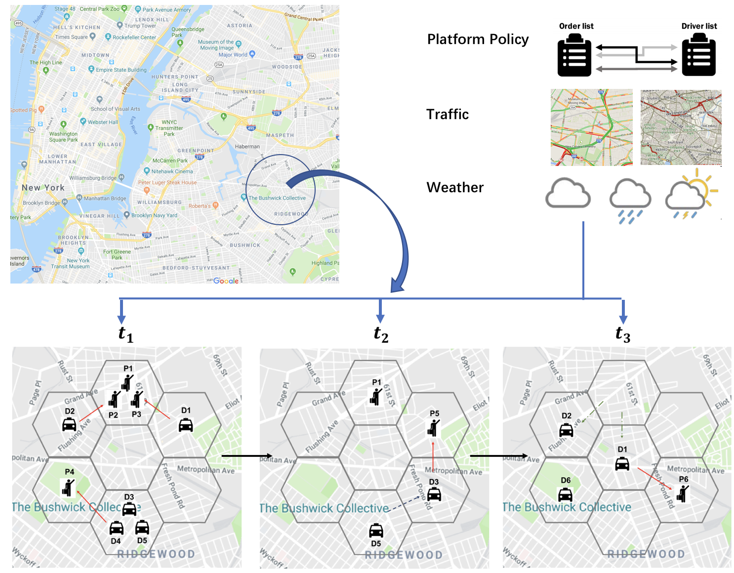
Figure 1: Dynamic supply and demand networks at three time points in a representative ride-sourcing platform. We divide the whole city into multiple hexagon areas.

Large volumes of data collected from multiple spatio-temporal networks are increasingly studied in diverse fields including climate science, social sciences, neuroscience, epidemiology, and transportation. In addition, those spatio-temporal networks may interact with each other across spatial and/or temporal dimension. A typical example is that the dynamic demand and supply networks of a ride-sourcing platform (Wang & Yang, 2019) are two sequences of un-normalized masses measured on the same undirected (or directed) graph $G=(\mathbb{V},\mathbb{E})$, where $\mathbb{V}$ and $\mathbb{E}$ are, respectively, a vertex set and a set of edges connecting vertex pairs. Figure 1 illustrates how the two complicated networks interact with each other and evolve over time. Specifically, a city is divided into hundreds of non-overlapping grids as the vertex set $\mathbb{V}$ with the edge structure $\mathbb{E}$ determined by road networks and location functionalities. Both demands and supplies are observed across grids at each time window with possibly different total masses and distributions. The ride-sourcing platform uses some order dispatching policy to match customer requests with possible surrounding idle drivers, while after finishing serving assigned orders, drivers return back to the supply pool to prepare for the next feasible matching. The aim of this paper is to address a fundamental question of interest for the demand and supply networks of two-sided markets.

The fundamental question of interest that we consider here is how to quantify the spatial equilibrium of dynamic supply-demand networks for two-sided markets, particularly ride-sourcing platforms (e.g., Uber and DiDi). To solve this question, we first introduce a weighted graph structure $(G,W,C)$ to characterize the transport network and transport costs of a city. Specifically, we divide each market into $N$ disjoint areas and regard them as vertices, denoted as $\mathbb{V}=\{v_{1},\ldots,v_{N}\}$. Let $\mathbb{E}$ be a set of edges between any possible pair of vertices such that $(v_{i},v_{j})\in\mathbb{E}\subset\mathbb{V}\times\mathbb{V}$ is an edge equipped with an nonegative weight $w_{ij}$ (e.g., transportation cost). For all $(v_{i},v_{j})\notin\mathbb{E},$ we set $w_{ij}=\infty$. The weighted graph structure consists of an undirected (or directed) graph $G=(\mathbb{V},\mathbb{E})$ as well as a weight matrix $W=(w_{ij})$, where $w_{ij}$s’ are nonegative weights. A graph-based transport cost from $v_{i}$ to $v_{j}$ is defined as $c_{ij}=\min_{K\geq 0,(i_{k})_{k=0}^{K}:v_{i}\rightarrow v_{j}}\{\sum_{k}w_{i_{k},i_{k+1}}:\forall k\in[\![0,K-1]\!],(v_{i_{k}},v_{i_{k+1}})\in\mathbb{E}\},$ where $(i_{k})_{k=0}^{K}:v_{i}\rightarrow v_{j}$ denotes any path on $G$ through $\mathbb{E}$ starting from $v_{i_{0}}=v_{i}$ and ending at $v_{i_{K}}=v_{j}$. Thus, $c_{ij}$ is the geodesic distance from $v_{i}$ to $v_{j}$ or the minimal cost of transporting one unit of object from $v_{i}$ to $v_{j}$. Thus, we can define a transport cost matrix on $(G,W)$, denoted as $C=(c_{ij})\in R^{N\times N}$. The $C$ may be time variant, since it depends on the real-time traffic and weather conditions for ride-sourcing platform. The $C$ is possibly asymmetric since the graph $G$ can be directed.

Second, we need to introduce a distance (or metric) to quantify the difference between demand and supply masses at each time interval and across time on $(G,W,C)$. At a given time interval, we define $\nu_{j}=\nu(v_{j})$ and $\mu_{j}=\mu(v_{j})$ as the point masses at vertex $v_{j}$ for the two measures $\nu$ and $\mu$, which, respectively, represent the number of customer requests and available drivers inside the vertex $v_{j}$ of the ride-sourcing platform (Wang & Yang, 2019). The supply and demand systems at each timestamp can be modeled as two discrete Lebesgue measures $\mu$ and $\nu$ on $(G,W,C)$ with locally finite masses such that $\max(\mu(\mathbb{V}_{0}),\nu(\mathbb{V}_{0}))$ is finite for every compact set $\mathbb{V}_{0}\subset\mathbb{V}$. We consider a general case that the two measures can be unbalanced, that is, $\mathbf{\mu}=\sum_{i=1}^{N}\mu_{i}$ and $\mathbf{\nu}=\sum_{i=1}^{N}\nu_{i}$ may be unequal to each other. Defining a metric between $\mu$ and $\nu$ falls into the field of optimal transport.

Optimal transport has been widely studied in diverse disciplines, such as statistics, applied mathematics, medical imaging, and computer vision. Wasserstein-based metrics based on the mathematics of optimal mass transport have been proved to be powerful tools for comparing objects in complex spaces. Some successful applications include solving transport partial differential equation (PDE) (Ambrosio & Gangbo, 2008), imaging processing (Rabin & Papadakis, 2015), statistical inference in machine learning (Solomon et al., 2014), manifold diffeomorphisms (Grenander & Miller, 2007), and serving as the cost function for training Generative Adversarial Networks (Arjovsky et al., 2017), among many others. However, existing Wasserstein-based metrics are not directly applicable to the comparison of two unbalanced measures defined on $(G,W,C)$ as detailed in Section 2.1.

We introduce a graph-based equilibrium metric (GEM) and formulate it as an unbalanced optimal transport problem. Our main contributions are summarized as follows. First, we propose a novel GEM, which can be regarded as a restricted generalized Wasserstein distance, to quantify the distance between dynamic demand and supply networks on the weighted graph structure. It not only allows the optimal transport guided by asymmetric costs and node connections, but also accounts for unbalanced masses. It also allows one of the two sides (supplies) to play the transporting role and the other (demands) to be fixed, which satisfies the physical interpretation of ride-sourcing platforms. Second, varying the size of each vertex leads to multilevel GEMs and their corresponding optimal transport functions. At the finest scale, our GEM reduces to solving an unbalanced assignment problem and its corresponding optimal transport function contains many local details. In contrast, at a relatively coarse scale, it gives a coarse representation (or low frequency patterns) of the optimal transport function. Third, numerically, the calculation of GEM can be reformulated as a standard linear programing (LP) problem. Theoretically, we investigate several theoretical properties of GEM including the convergence of the LP algorithm for computing GEM, the expectation of GEM, and the metric property, additive property and weak convergence of GEM. Fourth, we apply GEM to the ‘supply-demand diagnostic data set’ obtained from the DiDi Chuxing in order to address some important operational tasks, such as the prediction of the efficiency of a given dispatching policy.

The remainder of this paper is structured as follows. Section 2 develops graph-based equilibrium metrics and their computational approach, while discussing their potential applications. Section 3 studies four theoretical properties associated with GEM. Section 4 demonstrates the applications of GEM in the intelligent operations of DiDi Chuxing.

2 Methodologies

2.1 Existing Wasserstein-type Distances

Many approaches have been proposed to measure the distance between two measures (or distributions) on a metric space. Most of them fall into two broad categories including the aggregation of pixel-wise differences and the transport cost of moving one measure to match the other. Measurements in the first category include the $L_{p}$-distance, the Total Variation (TV) distance, and the Kullback-Leibler (KL) divergence (Cha, 2007), among others. A typical example is the Hellinger Distance reviewed as follows.

Definition 2.1.

(Hellinger Distance) Let $M(X)$ and $M_{+}(X)$ be the vector space of Radon measures and the cone of nonnegative Radon measures on a Hausdorff topological space $X$. Then, we use $\mu$ and $\nu$ to denote two probability measures that are absolutely continuous with respect to a third probability measure $\nu_{0}$. The square of the Hellinger distance between $\mu$ and $\nu\in M_{+}(X)$ is defined as $D_{H}^{2}(\mu,\nu)=0.5\int_{X}\left({\sqrt{d\mu/d\nu_{0}}}-{\sqrt{d\nu/d\nu_{0}}}\right)^{2}d\nu_{0},$ where $d\mu/d\nu_{0}$ and $d\nu/d\nu_{0}$ are the Radon-Nikodym derivatives of $\mu$ and $\nu$, respectively.

All these metrics suffer from two major issues. Please refer to Figures 2 for details. First, all these metrics not only fail to consider the connections among different locations (vertices in graph), but also ignore the topological (or geometric) structure of $X$. Second, the use of Hellinger-type distances requires a normalization step to enforce $\mu(X)=\int_{X}d\mu=\nu(X)=\int_{X}d\nu$, which can create a false balance issue.

To address these two issues, the second category of metrics, such as the Wasserstein distance (Villani, 2008), is proposed by solving an optimal transport problem. In the real world, original supply resources can usually be transported to achieve a better equilibrium between $\mu$ and $\nu$. All those distances have deep connections to well studied assignment problems from combinatorial optimization (Steele, 1987).

Definition 2.2.

(Wasserstein Distance) Let $X$ and $Y$ be Hausdorff topological spaces and $X\times Y$ be their product space. We introduce a lower semi-continuous function $c:X\times Y\rightarrow R\cup\{\infty\}$, an nonnegative measure (or a transport function) $\gamma\in M_{+}(X\times Y)$, and an equality constraint $\iota_{\{=\}}(\alpha|\beta)$ which is $0$ if $\alpha=\beta$ and $\infty$ otherwise. Then the optimal transport problem for measures $\mu\in M_{+}(X)$ and $\nu\in M_{+}(Y)$ with the same total masses, that is $\mu(X)=\nu(Y)$, can be defined as

$$D_{W}(\mu,\nu|c)=\inf_{\gamma\in M_{+}(X\times Y)}\left\{\int_{X\times Y}cd\gamma+\iota_{\{=\}}(P^{X}_{\#}\gamma|\mu)+\iota_{\{=\}}(P^{Y}_{\#}\gamma|\nu)\right\},$$ (1)

where $P^{X}_{\#}\gamma$ and $P^{Y}_{\#}\gamma$ denote the first and second marginals of $\gamma$, respectively.

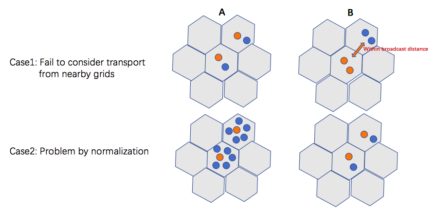
Figure 2: Examples of supply-demand networks for illustrating the limitations of Hellinger distance: blue and orange objects represent orders and idle drivers, respectively. The first row illustrates the consequence of not transporting objects into nearby vertices. Specifically, the left one has a zero Hellinger distance, whereas the right one has a nonzero Hellinger distance without transporting the two drivers into the nearby vertex with two orders. The second row illustrates that the normalization step can remove the imbalance between orders and idle drivers. Specifically, the left one has a large imbalance between orders and idle drivers, whereas after the normlization, the right one has a zero Hellinger distance.

Intuitively, $\gamma$ denotes a transport plan, measuring how far you have to move the mass of $\mu$ to turn it into $\nu$. Standard optimal transport in (1) is only meaningful whenever $\mu$ and $\nu$ have the same total masses. Whenever $\mu(X)\not=\nu(Y)$, there is no feasible $\gamma$ in (1). For the real-world ride-sourcing platforms, however, it is important to compute some sort of relaxed transportation between two arbitrary non-negative measures. An improved approach is to build an unbalanced optimal transport problem by introducing two divergences over $X$ and $Y$, denoted as $\mathcal{D}_{\varphi_{1}}$ and $\mathcal{D}_{\varphi_{2}}$, respectively (Chizat et al., 2018; Liero et al., 2018).

Definition 2.3.

(Divergences). Let $\varphi$ be an entropy function. For $\mu,\nu\in M(T)$, $\frac{d\mu}{d\nu}\nu+\mu^{\bot}$ is the Lebesgue decomposition of $\mu$ with respect to $\nu$. The divergence $D_{\varphi}$ is defined by $D_{\varphi}(\mu|\nu):=\int_{T}\varphi(\frac{d\mu}{d\nu})d\nu+\varphi_{\infty}^{\prime}\mu^{\bot}(T)$ if $\mu$ and $\nu$ are nonnegative and $\infty$ otherwise.

Now, we can give the formal definition of Generalized Wasserstein Distance.

Definition 2.4.

(Generalized Wasserstein Distance (GWD)) Let $c:X\times Y\rightarrow[0,\infty]$ be a lower semi-continuous function, the unbalanced optimal transport problem is

$$D_{\varphi_{1},\varphi_{2}}(\mu,\nu|c)=\inf_{\gamma\in M_{+}(X\times Y)}\left\{\int_{X\times Y}cd\gamma+\mathcal{D}_{\varphi_{1}}(P^{X}_{\#}\gamma|\mu)+\mathcal{D}_{\varphi_{2}}(P^{Y}_{\#}\gamma|\nu)\right\}.$$ (2)

Different from standard Wasserstein Distance which normalizes the input measures into probability distributions, GWD quantifies in some way the deviation of the marginals of the transport plan $\gamma$ from the two unbalanced measures $\mu$ and $\nu$ by using $\varphi$-divergence. Although $D_{\varphi_{1},\varphi_{2}}(\mu,\nu|c)$ enjoys some nice properties, such as metric property (Chizat et al., 2018; Liero et al., 2018), the solution to (2), denoted as $\gamma_{*}$, may not have any physical meaning. For the ride-sourcing business, such $\gamma_{*}$ is critically important for assigning supplies to demands since it can be regarded as the graph representation of a dispatching policy. Therefore, the use of $D_{\varphi_{1},\varphi_{2}}(\mu,\nu|c)$ still cannot fully cover the ’useful’ relative size between $\mu$ and $\nu$, since it may underestimate unmatched resources by allowing some infeasible transports, that is, the space $M_{+}(X\times Y)$ is too large to be useful. Three major issues of using $D_{\varphi_{1},\varphi_{2}}(\mu,\nu|c)$ are given as follows. The first issue is that in many applications (e.g., ride-sourcing platform), point masses in only one of the two measures are allowed to be transported and those in the other measure are fixed. In this case, the symmetric property does not hold. The second issue is that neither $W$ nor $C$ can be used to define a standard metric space on $G=(\mathbb{V},\mathbb{E})$, since transport cost (or weight) matrix may not satisfy the three key assumptions of standard metrics. For instance, the transport cost from $v_{i}$ to $v_{j}$ may be unequal to that from $v_{j}$ to $v_{i}$, since transport cost matrix $C\in R^{N\times N}$ can be asymmetric for directed graphs. Moreover, the direct transport cost from $v_{i}$ to $v_{j}$ may be larger than or equal to the sum of the transport cost from $v_{i}$ to $v_{k}$ and that from $v_{k}$ to $v_{j}$. The third issue is that in some applications, such as supply-demand networks, the transport cost from $v_{i}$ to $v_{j}$ may not be a constant and the transport cost from a vertex to itself may not be zero. It is possible that supply units at vertex $v_{i}$ have their individual transport costs of moving within/outside the vertex $v_{i}.$ Subsequently, their transport costs from $v_{i}$ to $v_{j}$ may follow a distribution instead of being a constant.

2.2 Graph-based Equilibrium Metrics

On $(G,W,C)$, we formally introduce our GEMs for two discrete measures $\mu$ and $\nu$ in $M_{+}(\mathbb{V})$, among which point masses in $\mu$ are allowed to be transported and those in $\nu$ are fixed. We need to introduce some notations. In this case, we have $X=Y=\mathbb{V}$ and use $P^{V}_{\#1}\gamma$ and $P^{V}_{\#2}\gamma$ to represent $P^{X}_{\#}\gamma$ and $P^{Y}_{\#}\gamma$, respectively. Let $|\mu|=\sum_{i=1}^{N}\mu(v_{i})$ and $|\mu-\tilde{\mu}|=\sum_{i=1}^{N}|\mu(v_{i})-\tilde{\mu}(v_{i})|$. For $i=1,\ldots,N$, we use ${\mathcal{N}}_{i}$ to denote the neighboring set of $v_{i}$ in $\mathbb{V}$, which contains $v_{i}$ and its (possibly high-order) neighboring vertexes. Moreover, $v_{i}\in\mathcal{N}_{j}$ does not ensure $v_{j}\in\mathcal{N}_{i}$ since the traffic and road networks may constrain directly transporting cars from $v_{j}$ to $v_{i}$.

Let $c:\mathbb{V}\times\mathbb{V}\rightarrow R\cup\{\infty\}$ be a function and $\gamma\in M_{+}(\mathbb{V}\times\mathbb{V})$ be a nonnegative measure. The general form of our GEM on $(G,W,C)$ is written as

$$\rho_{\lambda}(\mu,\nu|G,C)=\inf_{\tilde{\mu}\in M_{+}(\mathbb{V}),\gamma\in M_{+}(\mathbb{V}\times\mathbb{V})}\left\{|\nu-\tilde{\mu}|+\lambda\int_{\mathbb{V}\times\mathbb{V}}cd\gamma\right\}$$ (3)

subject to an equality constraint and two sets of transport constraints given by

$$|\mu|=|\tilde{\mu}|,~{}~{}~{}~{}(P^{V}_{\#1}\gamma)(v_{i})=\sum_{v_{j}\in\mathcal{N}_{i}}\gamma(v_{i},v_{j})=\mu_{i}\,\,\,\,\,\text{and}\,\,\,\,\,(P^{V}_{\#2}\gamma)(v_{i})=\sum_{v_{i}\in\mathcal{N}_{j}}\gamma(v_{j},v_{i})\,=\tilde{\mu}_{i},$$ (4)

where $\lambda$ is a non-negative hyper-parameter. The three sets of constraints in (4) ensure that $\tilde{\mu}$ shares the same total mass with $\mu$ and $\gamma$ transports $\mu$ to $\tilde{\mu}$. Thus, the feasible set for (4) is much smaller than that for (2). The integration of $\lambda\int_{\mathbb{V}\times\mathbb{V}}cd\gamma$ and the three sets of constraints in (4) is equivalent to the balanced Wasserstein distance in (1), so GEM is the integration of the balanced Wasserstein distance and the $L_{1}$ norm.

In our GEM framework, one of the two measures plays the role of ’predator’ to move and ’catch’ the ’prey’, which mimics the general supply-demand system of ride-sourcing platforms. Therefore, different from the setting of Piccoli & Rossi (2014), in which both two measures are rescaled, we fix $\nu$ but change $\mu$ only to make the two sides match each other under the asymmetric distance and transport range constraints. In Figure 3, we consider two simple examples in order to understand the differences between GEM and GWD. Moreover, since we only consider the transport from $\mu$ to $\tilde{\mu}$ with $\nu$ fixed, $\rho_{\lambda}(\mu,\nu|G,C)$ is generally asymmetric and can be regarded as a restricted GWD.

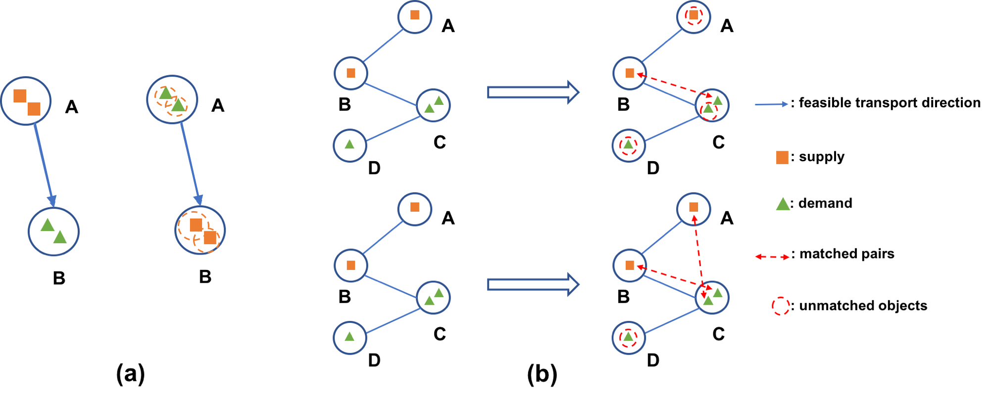
Figure 3: Examples illustrating the differences between GEM and GWD. Panel (a): For GEM, the four units can be matched in the left sub-figure, whereas it is infeasible in the right one. There exits a directed edge from A to B, but not from B to A. Panel (b): In the top sub-figure, one ‘demand’ unit at vertex C cannot be matched (the upper line) for GEM since the transport from vertex A to vertex C is not allowed in this case, whereas in the bottom sub-figure, they can be transported for GWD. In panel (b), for GEM, it is assumed that the neighboring set $\mathcal{N}_{i}$ only includes the adjacent vertexes of each vertex.

Besides GEM, the optimal solution of $(\tilde{\mu},\gamma)$ to (3), denoted as $(\tilde{\mu}_{*},\gamma_{*})$, also plays an important role in various two-sided markets, such as ride-sourcing platforms and E-commerce. The $\tilde{\mu}_{*}$ can be regarded as an optimal dispatch of transporting supplies $\mu$ to match demands $\nu$, whereas $\gamma_{*}$ is an optimal transport function associated with $\rho_{\lambda}(\mu,\nu|G,C)$. If we vary the area of each vertex from the coarsest to the finest scale, then we obtain multilevel GEM and its transport function. At the finest scale, our GEM reduces to solving an unbalanced assignment problem, so $\gamma_{*}$ is able to capture the local structure of the optimal transport function. In contrast, at a relatively coarse scale, we obtain a coarse representation of the optimal transport function, reflecting its global patterns. We will discuss how to apply GEM to ride-sourcing platforms in Section 2.4.

Furthermore, we can simplify $\gamma$ by defining $\gamma=(\gamma_{ij})$ as an $N\times N$ flow matrix with $\gamma_{ij}$ being the transport amount from $v_{i}$ to $v_{j}$. Let $\Gamma$ represent the set consisting of all the feasible solutions $\gamma$ with all non-negative elements $\gamma_{ij}\geq 0$. Let $\widetilde{\bm{\mu}}=(\widetilde{\mu}_{1},\ldots,\widetilde{\mu}_{N})^{T}\in R^{N}$ represent the measure $\mu$ after transporting $\gamma$ such that $\widetilde{\mu}_{i}=\sum_{v_{j}\in\mathcal{\mathcal{N}}_{i}}\gamma_{ji}$ holds for all $i$. Thus, our GEM is equivalent to solving a discrete optimization problem as follows:

$$\rho_{\lambda}(\mu,\nu|G,C) = \min_{\gamma\in\Gamma}\{\parallel\bm{\nu}-\widetilde{\bm{\mu}}\parallel_{1}+\lambda\sum_{v_{i}\in\mathbb{V}}\sum_{v_{j}\in\mathbb{V}}c_{ij}\gamma_{ij}\}$$

subject to $$\sum_{v_{j}\in{\mathcal{N}}_{i}}\gamma_{ij}=\mu_{i},\,\,\,\,\sum_{v_{j}\notin{\mathcal{N}}_{i}}\gamma_{ij}=0,\text{ and}\,\,\,\,\widetilde{\mu}_{i}=\sum_{v_{i}\in\mathcal{\mathcal{N}}_{j}}\gamma_{ji}\text{ for}\,\,\,\,\forall v_{i}\in\mathbb{V},$$

where $\bm{\nu}=(\nu_{1},\ldots,\nu_{N})^{T}\in R^{N}$ and $\parallel\cdot\parallel_{1}$ corresponds to the $L_{1}$ norm. Moreover, $\parallel\bm{\nu}-\widetilde{\bm{\mu}}\parallel_{1}$ in (2.2) is equivalent to the first term of the objective function in (3).

There are two key advantages of using the derived form given in (2.2) compared to the existing unbalanced optimal transport problem. The first one is that transport is only allowed between a vertex $v_{i}$ and its neighboring set $\mathcal{N}_{i}$ based on $G$.

The second one is that $\lambda$ can balance the transport cost taken to reallocate point masses and the requirement of assigning $\mu$ to satisfy $\nu$. The choice of $\lambda$ in practice is data-driven. To ensure that the transport only happens among selected vertex pairs under the optimal transport plan, the theoretical upper bound of $\lambda$ is $2/\max_{v_{i}\in V,v_{j}\in\widetilde{\mathcal{N}}_{i}}(c_{ij})$, where $\widetilde{\mathcal{N}}_{i}\subset\mathcal{N}_{i}$ contains all the neighboring vertexes of $v_{i}$ that transport from $v_{i}$. In this case, the cost of transporting one unit of supply from vertex $v_{i}$ to $v_{j}\in\widetilde{\mathcal{N}}_{i}$, $\lambda c_{ij}$, is smaller than its contribution to reducing $\parallel\bm{\nu}-\widetilde{\bm{\mu}}\parallel_{1}$, which is $2$ ($1$ for $v_{i}$ and $v_{j}$, respectively), when $\nu_{j}-\mu_{j}\geq 1$ and $\mu_{i}-\nu_{i}\geq 1$. Transport from $v_{i}$ to $v_{j}$ keeps decreasing the objective value $\rho_{\lambda}(\mu,\nu|G,C)$ until either the balance in the destination vertex $v_{j}$ or that in the origin vertex $v_{i}$ is achieved. In the real world, we usually let $\lambda\max_{v_{i}\in V,v_{j}\in\widetilde{\mathcal{N}}_{i}}(c_{ij})$ fall into the range $[0.4,0.5]$ with $c_{ij}$ being the geological distance and $\widetilde{\mathcal{N}}_{i}$ containing all the first-order adjacent vertexes of $v_{i}$ in $(G,W,C)$, which can achieve the best performance in some problems, such as the prediction of order answer rate.

2.3 Computational Approach

Optimal solution $\gamma^{*}$ to (2.2) can be calculated by solving a standard linear programming (LP). We will reformulate (2.2) as a LP problem and then use a revised simplex method incorporated in a C package GNU Linear Programming Kit (GLPK) to solve (2.2). We have found that GLPK works pretty well in our real data analyses in Section 4.

We need to introduce some notations. Since the transport range constraints in (4) impose $\gamma_{ij}=0$ for $v_{j}\notin{\mathcal{N}}_{i}$, we only need to assign optimal values to $\widetilde{\gamma}=\mbox{Vec}\{\gamma_{ij},j\in{\mathcal{N}}_{i}\}\in R^{N_{0}\times 1}$, where $N_{0}=\sum_{i=1}^{N}n_{i}$ and $\mbox{Vec}(\cdot)$ denotes the vectorization of a matrix. With this simplification, the dimension of solvable variables is reduced from $O(N^{2})$ to $O(N_{0})$, which highly increases the computational efficiency of our algorithm. Let $A_{1}$ and $A_{2}$ be two $N\times N_{0}$ matrices. The $i$-th row of $A_{1}$ consists of $0$’s except the $(\sum_{j=1}^{i-1}n_{j}+1)$-th to $(\sum_{j=1}^{i}n_{j})$-th elements being $1$. Similarly, all the elements of of $i$-th row of $A_{2}$ are zeros except the $(\sum_{p=1}^{j-1}n_{p}+q)$-th element being $1$ when grid $v_{i}$ is indexed by $q$ in the neighboring set ${\mathcal{N}}_{j}$ of vertex $v_{j}$. Let $\widetilde{C}\in R^{N_{0}\times 1}$ be the vector including the unit transport costs for all the corresponding ${\gamma_{ij}}^{\prime}s\in\widetilde{\gamma}$. Moreover, we define

$$A=\begin{bmatrix}A_{1}&{\bf 0}&{\bf 0}&{\bf 0}||A_{2}&{\bf I}_{N}&-{\bf I}_{N}&{\bf 0}||A_{2}&-{\bf I}_{N}&{\bf 0}&{\bf I}_{N}\end{bmatrix}~{}~{}~{}\mbox{and}~{}~{}~{}{\bf b}=\begin{bmatrix}\bm{\mu}^{T},\bm{\nu}^{T},\bm{\nu}^{T}\end{bmatrix}^{T},$$

where $\bm{\mu}=(\mu_{1},\ldots,\mu_{N})^{T}$, $A\in R^{3N\times(N_{0}+3N)}$, ${\bf b}\in R^{3N}$, and ${\bf I}_{N}$ is an identity matrix.

The (2.2) is equivalent to $\min\{\parallel\bm{\nu}-A_{2}\widetilde{\gamma}\parallel_{1}+\lambda\widetilde{C}^{T}\widetilde{\gamma}\}$ subject to $A_{1}\widetilde{\gamma}=\bm{\mu}$ and $\widetilde{\gamma}\geq 0.$ Let $S\in R^{N\times 1}$, it can be further transferred into a standard linear programming (LP)

$$\min\{\mathbf{1}^{T}S+\lambda\widetilde{C}^{T}\widetilde{\gamma}\}~{}~{}~{}\text{subject to}$$ (6)

$$A_{1}\widetilde{\gamma}=\bm{\mu},~{}A_{2}\widetilde{\gamma}+S\geq\bm{\nu},~{}A_{2}\widetilde{\gamma}-S\leq\bm{\nu},~{}\widetilde{\gamma}\geq 0,~{}~{}\text{and}~{}~{}S\geq 0.$$

The above LP can be further rewritten as

$$\min_{X}\{B^{T}X\}~{}~{}~{}~{}\text{subject to}\,\,AX={\bf b},\,\,\,X\geq 0,$$ (7)

where $B=(\lambda\widetilde{C}^{T},{\bf 1}^{T},{\bf 0}^{T},{\bf 0}^{T})^{T}$ and $X=(\widetilde{\gamma}^{T},S^{T},\bm{w}_{1}^{T},\bm{w}_{2}^{T})^{T}$, in which $\bm{w}_{1}$ and $\bm{w}_{2}$ are vectors of slack variables. The dual of (7) is assigned as

$$\max_{\textbf{y}\in R^{3N}}\{{\bf b}^{T}\textbf{y}\}~{}~{}~{}~{}\text{subject to}\,\,A^{T}\textbf{y}\leq B,$$ (8)

which further reduces the variable dimension from $N_{0}+3N$ to $3N$.

2.4 Applications of GEM in Ride-sourcing Platforms

To calculate GEM, we need to build a dynamic weighted graph structure over time for each city on the ride-sourcing platform as follows. We first divide a city into $|\mathbb{V}|=N$ non-overlapping hexagons and regard each hexagon as a vertex in $\mathbb{V}$. Then, we set $\mathcal{N}_{i}=\cup_{k=0}^{2}{\mathcal{N}}_{i}^{k}$, where ${\mathcal{N}}^{k}_{i}$ includes all the neighboring hexagons within the $k$-th outer layer of $v_{i}$ for $k>1$ and ${\mathcal{N}}^{0}_{i}$ only includes $v_{i}$ itself. A vertex $v_{j}$ belongs to the $k$-th outer layer of $v_{i}$ if $k$ steps are required to walk from $v_{i}$ to $v_{j}$ on the hexagonal network. Thus, we determine $G=(\mathbb{V},\mathbb{E})$. Second, we set $W_{t}=(w_{ijt})$, where $w_{ijt}$ is the distance between $v_{i}$ and $v_{j}$ in the $t-$th timestamp. Note that $w_{ijt}$ may vary with time due to the real-time locations of drivers and customers. Third, we compute $C_{t}=(c_{ijt})$ by using $W_{t}$ in the $t-$th timestamp. Finally, we obtain the dynamic weighted graph structure $(G,W_{t},C_{t})$.

We show how to use GEM to address three operational tasks of interest in ride-sourcing platforms. First, we can measure the optimal distance between observed dynamic supply and demand networks across time. We extract the spatio-temporal data $\textbf{O}=\{(o_{it})\}_{t}$ and $\textbf{D}=\{(d_{it})\}_{t}$ from the dynamic demand and supply systems, where $o_{it}$ and $d_{it}$ represent demands and supplies at vertex $v_{i}$ in the $t$-th timestamp, respectively. Given O and D, we set $\mu_{t}=(d_{it})_{i}$ and $\nu_{t}=(o_{it})_{i}$ and use the LP algorithm to calculate $\rho(t)=\rho_{\lambda}(\mu_{t},\nu_{t}|G,C_{t})$ and its corresponding solution, denoted as $(\tilde{\mu}_{t*}=(\tilde{d}_{it*})_{i},\gamma_{t*})$, in the $t$-th timestamp.

Furthermore, we introduce an optimal supply-demand ratio at each $v_{i}$ in the $t-$th timestamp defined as the ratio of $o_{it}$ over the ’optimal’ supplies $\tilde{d}_{it*}+\iota_{\{=\}}(\tilde{d}_{it*}=0)$, denoted as $\mbox{DSr}_{it}$, in which we add an extra term $\iota_{\{=\}}(\tilde{d}_{it*}=0)$ to avoid zero in the denominator. Similarly, we can define an optimal supply-demand difference as $\mbox{DSd}_{it}=o_{it}-\tilde{d}_{it*}$ at each $(v_{i},t)$. It allows us to create the spatiotemporal map of GEM-related measures $(\mbox{DSr}_{it},\mbox{DSd}_{it})$. Furthermore, we extend $(\mbox{DSr}_{it},\mbox{DSd}_{it})$ to a wide timespan $\mathcal{T}_{0}$ within a large region $\mathbb{V}_{0}\in\mathbb{V}$. For instance, we define a weighted average supply-demand ratio over $\mathbb{V}_{0}$ in $\mathcal{T}_{0}$ and a weighted average absolute supply-demand difference over $\mathbb{V}_{0}$ in $\mathcal{T}_{0}$ as follows:

$$\mbox{DSr}_{\mathcal{T}_{0}}(\mathbb{V}_{0})=\frac{\int_{t\in\mathcal{T}_{0}}\sum_{i\in\mathbb{V}_{0}}w_{it}\mbox{DSr}_{it}dt}{\int_{t\in\mathcal{T}_{0}}\sum_{i\in\mathbb{V}_{0}}w_{it}dt}~{}~{}\mbox{and}~{}~{}\mbox{ADSd}_{\mathcal{T}_{0}}(\mathbb{V}_{0})=\frac{\int_{t\in\mathcal{T}_{0}}\sum_{i\in\mathbb{V}_{0}}w_{it}|\mbox{DSd}_{it}|dt}{\int_{t\in\mathcal{T}_{0}}\sum_{i\in\mathbb{V}_{0}}w_{it}dt},$$ (9)

in which we set $w_{it}$ as either $o_{it}$ or $(o_{it}+\tilde{d}_{it*})/2$ in order to highlight vertices with high demands. A good market equilibrium in ride-sourcing platforms corresponds to small values of $|\mbox{DSd}_{it}|$ and $|\mbox{DSr}_{it}-1|$ across all $(v_{i},t)$. Please see Section 4.1 for details.

Second, we can use historical supply-demand information contained in $\{(\mbox{DSr}_{it},\mbox{DSd}_{it}):(v_{i},t)\in\mathbb{V}\times\mathcal{T}_{0}\}$ to design order dispatching policies for large-scale ride-sourcing platforms. Order dispatch is an essential component of any ride-sourcing platform for assigning idle drivers to nearby passengers. Standard order dispatching approaches focus on immediate customer satisfaction such as serving the order with the nearest drivers (Liao, 2003) or the first-come-first-go strategy to serve the order on the top of the waiting list with the first driver becoming available (Zhang & Pavone, 2016). Those greedy methods, however, fail to account for the spatial effects of an order and driver (O-D) pair on the other O-D pairs. Thus, they may not be optimal from a global perspective. To improve users’ experience, some more advanced techniques strive to balance between small pick-up distance and large drivers’ revenue. To design better dispatching policy, we will include additional historical supply-demand network information based on GEM to delineate its effects on the average expected gain from serving current order. Please see Section 4.2 for details.

Third, an important application of $\{\rho(t)\}$ is to use it as a metric to directly compare two (or more) dispatching policies for ride-sourcing platforms. The key idea is to detect whether there exists a significant difference between two sets of GEMs for two competitive policies under the same platform environment. Given the joint distribution of demand and supply in the platform, the smaller GEM is, the better many global operational metrics, such as order answer rate, order finishing rate, and driver’s working time, are. Compared with those global operational metrics, GEM is a more direct measurement of the operational efficiency for a ride-sourcing platform. Please see Section 4.3 for details.

3 Theoretical Properties

In this section, we study the theoretical properties of our GEM related methods proposed in Section 2, most of whose proofs can be found in the supplementary document.

First, we establish the convergence property of LP (7) for GEM.

Theorem 3.1.

The LP (7) has an optimal basic feasible solution. Furthermore, if $X$ is feasible for the primal problem (7) and y is feasible for the duality (8), then we have

$$\bar{z}=\textbf{y}^{T}{\bf b}=\textbf{y}^{T}AX\leq B^{T}X=z$$ (10)

If either (7) or (8) has a finite optimal value, then so does the other, the optimal values coincide, and the optimal solutions to both (7) and (8) exist.

An implication of Theorem 3.1 is that the LP algorithm for GEM converges. It demonstrates that there always exit theoretically optimal transport plans (including no transport case) to maximally increase the systematic coherence between the initially unbalanced supplies and demands. However, Theorem 3.1 also indicates that the optimal transport plan may not be unique considering the weighted graph structure and initial supply and demand distributions.

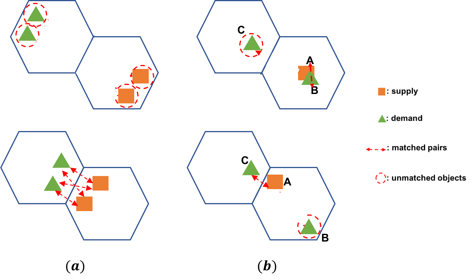
Figure 4: Two examples to illustrate the importance of using random $c_{ij}$. In Panel (a), two demands and two drivers can only be matched in the lower sub-figure since their corresponding pairs of distance are below a given threshold, whereas it is not the case in the upper sub-figure. In Panel (b), supply A is assigned to demand C in the lower sub-figure when the within-grid cost $c_{ii}$ is non-zero, and to demand B when $c_{ii}=0$, guided by the optimal transport plan with smaller transport costs.

Second, we carry out a probabilistic analysis of our LP (7) for GEM when $c_{ij}$ follows a distribution. Let’s start with two motivating examples of ride-sourcing platforms described in Figure 4. The $w_{ij}$ represents the geological distance or the traffic time, which may vary between each pair of supply at $v_{j}$ and demand at $v_{i}$. For the LP defined in (7), it is assumed that each component of $\widetilde{C}=(\tilde{c}_{1},\tilde{c}_{2},\ldots,\tilde{c}_{N_{0}})^{T}$ is a non-negative random variable, whereas all elements in $A$ and ${\bf b}$ in (7) are known. Let $z^{*}$ denote the minimum value of (7). Since $z^{*}$ is a function of $\widetilde{C}$, it is also a random variable. We provide an upper bound for the expectation of $z^{*}=z^{*}(\widetilde{C})$ below.

Theorem 3.2 (Expectation Bound).

Let $\tilde{c}_{1},\ldots,\tilde{c}_{N_{0}}$ be independent non-negative random variables. Suppose there exist $\alpha_{1}\in(0,\infty)$ and $\alpha_{2}\in(0,1]$ such that for $l=1,2,\ldots,N_{0}$ and all $h>0$ with $P(\lambda\tilde{c}_{l}\geq h)>0$, we have

$$E(\lambda\tilde{c}_{l}|\lambda\tilde{c}_{l}\geq h)\geq\alpha_{1}\lambda E(\tilde{c}_{l})+\alpha_{2}h,$$ (11)

where the expectation is taken with respect to $\tilde{c}_{l}$. Let $\{\hat{x}_{1},\ldots,\hat{x}_{3N+N_{0}}\}$ be any fixed feasible solution to (7). We have

$$E(z^{*})\leq{\alpha}_{2}^{-1}\{\sum_{l=1}^{N_{0}}(1-\alpha_{1}\delta_{l})E(\lambda\tilde{c}_{l})\hat{x}_{l}+\sum_{l=N_{0}+1}^{N_{0}+N}\hat{x}_{l}\},$$ (12)

where $\delta_{l}\in[0,1]$ defined in the supplementary document is a pre-defined nonnegative constant for each $l\in\{1,\ldots,N_{0}\}$.

Theorem 3.2 has at least two implications. First, condition (11) holds under some mild conditions. For instance, it can be shown that if $\tilde{c}_{j}$ is a bounded random variable that takes values in $[c_{j,L},c_{j,U}]$ such that $P(\tilde{c}_{j}>c_{j,L})>0$ and $\lim\inf_{h\rightarrow 0}h^{-1}P(\lambda\tilde{c}_{j}<h+\lambda c_{j,L})>0$, then condition (11) holds. Some examples of $\tilde{c}_{j}$ include uniform, truncated normal, and truncated exponential random variables, among others. For instance, we consider the case that $\tilde{c}_{j}$ follows Uniform $[c_{j,L},c_{j,U}]$. It can be shown that $E(\lambda\tilde{c}_{j}|\lambda\tilde{c}_{j}\geq h)=0.5(\lambda c_{j,U}+h)$, yielding $\alpha_{1}=c_{j,U}/(c_{j,U}+c_{j,L})$ and $\alpha_{2}=0.5$. Second, (12) gives an upper bound of the expected value of $z^{*}(\widetilde{C})$. If we set $\delta_{l}=0$ for all $l$, then we can obtain a larger upper bound compared with the right-hand side of (12). This result generalizes an existing result of Dyer et al. (1986) for standard linear programs with random costs under a stronger condition corresponding to $\alpha_{1}=1$.

Third, we examine the metric properties of $\rho_{\lambda}((\cdot),(\cdot)|G,C)$ including non-negativity, identity, symmetry, and the triangle inequality.

Theorem 3.3.

The operator $\rho_{\lambda}((\cdot),(\cdot)|G,C)$ is a semi-metric such that it satisfies non-negativity, identity, and symmetry, but not necessarily the triangle inequality when (i) $C=(c_{ij})\in R^{N\times N}$ is symmetric with $c_{ii}=0$ for all $i$;     (ii) $j\in\mathcal{N}_{i}$ if and only if $i\in\mathcal{N}_{j}$.

Theorem 3.3 indicates that if $C$ is symmetric, then $\rho_{\lambda}((\cdot),(\cdot)|G,C)$ as a semi-metric satisfies three properties including non-negativity, identity, and symmetry. Although the symmetric assumption of $C$ may be incorrect for all vertexes, it should be valid for most vertexes. Thus, $\rho_{\lambda}((\cdot),(\cdot)|G,C)$ is approximately a semi-metric.

Fourth, we give the upper and lower bounds of GEM and consider an additivity property in order to better understand how the transport costs and network structures affect GEM.

Theorem 3.4.

The following properties hold:

(i). $\left||\mu|-|\nu|\right|\leq\rho_{\lambda}(\mu,\nu|G,C)\leq(|\mu|+|\nu|)$

(ii). Additivity Property. For a non-negative $\Delta$, when $C$ is symmetric, we have

$$|\rho_{\lambda}(\mu,\nu+\Delta|G,C)-\rho_{\lambda}(\mu,\nu|G,C)|\leq N\Delta;\,\,\,\,|\rho_{\lambda}(\mu+\Delta,\nu|G,C)-\rho_{\lambda}(\mu,\nu|G,C)|\leq N\Delta.$$

Property (i) shows that GEM can be bounded from both above and below. Based on the additivity property, the GEM value can either increase or decrease with one-side node-wise augmentation, which depends on the weighted graph structure and the distribution of supply and demand. This indicates that applying proper stimulus at selected vertexes is more efficient than globally increasing supply resources.

Fifth, we examine the weak convergence property of $\rho_{\lambda}((\cdot),(\cdot)|G,C)$.

Theorem 3.5.

(Weak Convergence) Let $\{\mu_{n}\}$ be a sequence of measures on space $\mathbb{V}$, and $\mu_{n},\mu\in M_{+}(\mathbb{V})$. If all the transport costs are bounded, that is $c_{ij}\leq R\,\,$ holds for $\forall v_{i}\in\mathbb{V}$ and $v_{j}\in\mathcal{N}_{i}$, then $\rho_{\lambda}(\mu,\mu_{n}|G,C)\rightarrow 0$ when $\mu_{n}\rightarrow\mu$ and $\{\mu_{n}\}$ is tight.

Here is an immediate corollary of Theorem 3.5.

Corollary 3.5.1.

Let $\{\mu_{n}\}$ and $\{\nu_{n}\}$ be two sequences of measures on space $\mathbb{V}$, and $\mu_{n},\nu_{n},\mu,\nu\in M_{+}(\mathbb{V})$. If $c_{ij}\leq R$ holds for $\,\forall\,v_{i}\in\mathbb{V}$ and $v_{j}\in\mathcal{N}_{i}$, then we have

$$\text{if }\mu_{n}\,\,(resp.\,\nu_{n})\rightarrow\mu\,\,(resp.\,\nu)\text{ and }\{\mu_{n}\},\{\nu_{n}\}\text{ are tight, then }\,\rho_{\lambda}(\mu_{n},\nu_{n}|G,C)\rightarrow\rho_{\lambda}(\mu,\nu|G,C).$$

Theorem 3.5 states that the GEM value goes to $0$ and no transport is required when the initial distributions of $\mu$ and $\nu$ are getting close to each other.

4 Experiments

In this section, we apply GEM to the supply-demand diagnostic data set in order to address three important operational tasks in ride-sourcing platforms, including answer-rate prediction, the design of order dispatching strategy, and policy assessment. Without special saying, we use the method described in subsection 2.4 to construct the dynamic weighted graph structure across time in all these analyses. We have released the ‘supply-demand diagnostic data set’ through the DiDi GAIA Open Data Initiative at https://outreach.didichuxing.com/appEn-vue/dataList and made the computer codes together with necessary files available at https://github.com/BIG-S2/GEM.

4.1 Answer-Rate Prediction

The data set that we use here includes both demand and idle driver information from April 21st to May 20th, 2018 in a large city H. We divide the whole city into $N=800$ non-overlapping hexagonal sub-regions with side length being $1400$m to form the whole vertex set $\mathbb{V}$. We let the directed edge weight $w_{ij}$ from $v_{i}$ to $v_{j}\in{\mathcal{N}}^{1}_{i}$ be the distance between the centers of the two sub-regions, which is $2400$m if $v_{j}$ can be directly reached by $v_{i}$ through traffic without first passing through another vertex. Otherwise, $w_{ij}=\infty$. We compute the numbers of idle drivers and demands in each vertex per minute and then extract the dynamic supply-demand data set.

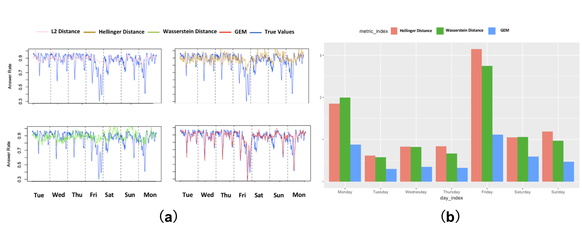
Figure 5: Results from the answer-rate prediction. Panel (a): comparisons of the log-value of real answer rates obtained from May 12th to May 18th, 2018 and their predictive values based on the $L_{2}$ distance, the Hellinger distance, the Wasserstein distance, and GEM. Panel (b): comparisons of day-wise RMSEs of answer rate prediction obtained from Monday to Sunday within the whole city area.

The aim of this data analysis is to examine whether the GEM-related measures, such as $\mbox{DSr}_{it}$, are useful for predicting order answer rate in ride-sourcing platforms. Order answer rate is defined as the number of orders accepted by drivers divided by the total number of orders in a fixed time interval. Specifically, we predict the log-value of order answer rate of the incoming 10 (or 60) minutes by using historical metric values. We computed the Hellinger distance, the $L_{2}$ distance, the Wasserstein distance, and GEM for each 10-minute interval. The $L_{2}$ distance is calculated by using the numbers of orders and available drivers in all vertices across 10 consecutive 1-min timestamps. The Hellinger distance is calculated by normalizing the numbers of orders and available drivers in all vertices and across 10 consecutive 1-min timestamps into probability distributions. For the Wasserstein distance, we first normalize both supplies and demands at each one-minute time interval into two probability distributions and calculate their corresponding Wasserstein distance. Subsequently, we obtain the metric value over each 10-minute interval by aggregating the Wasserstein distances computed across the 10 included one-minute timestamps by using their corresponding weights $\sum_{v_{i}\in V}o_{it_{k}}/\sum_{t_{k}\in\mathcal{T}}\sum_{v_{i}\in\mathbb{V}}o_{it_{k}}$. For GEM, we compute the supply-demand ratio map of $\mbox{DSr}_{it}$ per minute and then we calculate $\mbox{DSr}_{\mathcal{T}_{0}}(V)$ for each 10-minute interval.

We split the supply-demand data set into a training data set consisting of observations from April 26th to May 11th, 2018, and a test data set consisting of observations from May 12th to May 21st, 2018. We use linear regression models to predict the log-value of order answer rate of the incoming $j-$th 10 minutes for $j=1,\ldots,6$ by using various historical metric variables of the previous $p=10$ 10-minute snapshots and those in the same time windows of the previous $5$ days.

We use Mean Absolute Percentage Error (MAPE) and Root Mean Squared Error (RMSE) as evaluation metrics to examine the prediction accuracy of all the four compared metrics. Table 1 shows their corresponding RMSE and MAPE values based on the test data. Due to the space limitation, we only provide the results corresponding to those at $t+10$ and $t+60$ minutes, which indicate the short-term and long-term prediction capacities of all the four metrics. Moreover, we also include the results during the evening peak hours starting from 6 pm to 8 pm. For both the $t+10$ and $t+60$ cases, GEM significantly outperforms all other three metrics, which may not sufficiently capture the dynamic transport and systematic balance of the weighted graph structure.

Figure 5 (a) presents the real order answer rates and their predictive values in the last 7 test days (Tuesday to Monday) from May 12th to May 18th based on all the four metrics for the $(t+10)$ case. Compared with all other methods, GEM shows higher consistency between the true and predicted answer rate values, especially for some abnormal extreme cases. Furthermore, Figure 5 (b) presents the histograms of RMSEs for the Hellinger distance, the Wasserstein distance, and GEM at each day of the last seven dayes, indicating that GEM outperforms the other two metrics consistently in all seven days. Therefore, our GEM is able to capture the short- and long-term variability within the coherence between the two spatial-temporal systems and has strong prediction capacity for future answer rates.

4.2 Order Dispatching Policies

We consider the order dispatching problem of matching $N_{o}$ orders with $N_{d}$ available idle drivers, where $N_{o}$ and $N_{d}$ denote the total number of orders and that of idle drivers in the current timestamp, respectively. The edge weight $A(k,l)$ in the bipartite graph equals to the expected earnings when pairing driver $l$ to order $k$. Let $x_{kl}$ be 1 if order $k$ is assigned to driver $l$ and 0 otherwise. The global order dispatching algorithm solves a bipartite matching problem as follows:

$$\text{arg}\max_{x_{kl}}\sum_{k=0}^{N_{d}}\sum_{l=0}^{N_{o}}A(k,l)x_{kl},~{}\text{s.t.}\,\,\sum_{k=0}^{N_{d}}x_{kl}\leq 1\,\,\,\,\forall l;\,\,\sum_{l=0}^{N_{o}}x_{kl}\leq 1\,\,\forall k;x_{kl}=0\text{ if }c_{kl}>\epsilon~{}~{}\forall k,l.$$ (13)

See Figure 6 for a graphical illustration of (13). The constraints ensure that each order can be paired to at most one available driver and similarly each driver can be assigned to at most one order. In practice, only drivers within a certain distance could serve the corresponding orders, which means that $x_{kl}$s’ are forced to be $0$ when the distance between order $k$ and driver $l$, denoted as $c_{kl}$, is beyond the maximal pick-up distance $\epsilon$. The state-of-art algorithm to solve this kind of matching problem is the Kuhn-Munkres (KM) algorithm (Munkres, 1957), which will be used to solve the formulated problem here.

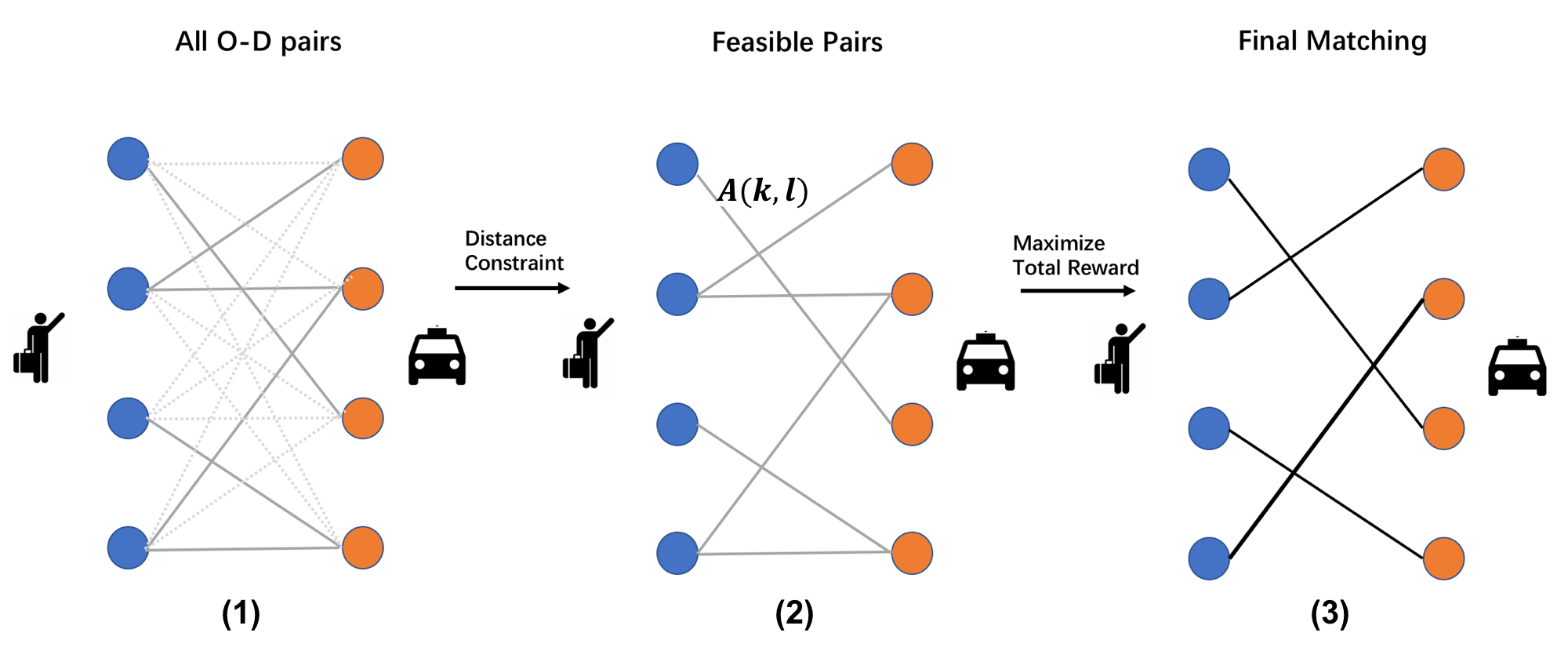
Figure 6: The order dispatch as a bipartite matching problem: (a) available orders and drivers prepared for pairing; (b) quantifying all the potential expected earning $A(k,l)$ for all driver-order pairs $(k,l)$ that satisfy the dispatching constraints; and (c) finding the optimal one-to-one bipartite matching in order to maximize the total revenue.

In this paper, we compare three different dispatching policies based on three different formulations of $A(k,l)$. The first one as a baseline only considers the immediate reward of assigning driver $l$ to order $k$, which is defined as $A^{(1)}(k,l)=\alpha_{1}r_{k}-\alpha_{2}c_{kl},$ where $r_{k}$ is the driver’s earning by serving order $k$ and $c_{kl}$ is the pick-up distance between order $k$ and driver $l$. Moreover, $\alpha_{1}$ and $\alpha_{2}$ are tuning parameters such that the two terms are balanced to maximize drivers’ salaries, while reducing customers’ waiting time.

The second one is given by $A^{(2)}(k,l)=\alpha_{1}r_{k}-\alpha_{2}c_{kl}+\alpha_{3}\{\eta^{\Delta t_{lk}}V_{1}(s^{\prime}_{lk})-V_{1}(s_{l})\},$ where $\eta$ is the discount factor and an additional term $\alpha_{3}\{\eta^{\Delta t_{lk}}V_{1}(s^{\prime}_{lk})-V_{1}(s_{l})\}$ is introduced to enhance the long-term effects of current actions on drivers’ future income (Xu et al., 2018). Let $V_{1}(s)$ be the expected earnings from now to the end of the day for a driver located at $s=(v,t)$, where $v\in\mathbb{V}$ and $t$ is the current time. Moreover, $s_{l}=(v^{(l)},t)$ and $s^{\prime}_{lk}=(v^{(k)},t+\Delta t_{lk})$ here represent the current spatial-temporal state of driver $l$ and his/her estimated finishing state when completing serving order $k$, where $v^{(l)}\in\mathbb{V}$ is the current region of driver $l$ before order assignment and $v^{(k)}\in\mathbb{V}$ is the destination region of order $k$ and $\Delta t_{lk}$ denotes the total time required for driver $l$ to finish the whole process of serving order $k$. If a driver becomes available to a new order immediately after finishing the ongoing one, then $\eta^{\Delta t_{lk}}V_{1}(s^{\prime}_{lk})-V_{1}(s_{l})$ is the extra future earning for driver $l$ by serving order $k$ other than staying idle.

The third one is given by $A^{(3)}(k,l)=A^{(2)}(k,l)+\alpha_{4}\{\eta^{\Delta t_{lk}}V_{2}(s^{\prime}_{lk})-V_{2}(s_{l})\},$ where $\alpha_{4}\{\eta^{\Delta t_{lk}}V_{2}(s^{\prime}_{lk})-V_{2}(s_{l})\}$ is introduced to balance the supply-demand coherence. Moreover, $V_{2}(s)=\nu_{t}(v)-\tilde{\mu}_{t}(v)$ at $s=(v,t)$ is calculated from GEM in (2.2). Using $V_{2}(\cdot)$ increases the probability that customers’ requests can be quickly answered by nearby drivers, whereas $V_{1}(\cdot)$ ignores the interaction effects when multiple drivers are heading to the same location. Thus, when the future demand has already been fulfilled by drivers re-allocated by previous completed servings, assigning more drivers might decrease $V_{1}(\cdot)$ in the target location.

We use a comprehensive and realistic dispatch simulator designed for recovering the real online ride-sourcing system to evaluate the three dispatching policies. The simulator models the transition dynamics of the supply and demand systems to mimic the real on-demand ride-hailing platform. The order demand distribution of the simulator is generated based on historical data. The driver supply distribution is initialized by historical data at the beginning of the day, and then evolves following the simulator’s transition dynamics (including drivers getting online/offline, driver movement with passengers and idle driver random movement) as well as the order dispatching policies. The differences between the simulated results and the real-world situation is less than 2% in terms of some important metrics, such as drivers’ revenue, answer rate, and idle driver rate.

To compare the three dispatching policies, we randomly selected a specific city S, which usualy has in total 150, 000 to 200, 000 ride demands per day. We still divide the whole city area into $N=800$ hexagonal vertices and use the geological distance between two nearby grids to be the edge weights. Furthermore, three different days including 2018/05/15 (Tuesday), 2018/05/18 (Friday), and 2018/05/19 (Saturday) were analyzed since the global order answer rates on weekday are usually much lower than those at weekend by looking at the historical data. Both $V_{1}(\cdot)$ and $V_{2}(\cdot)$ values were obtained by taking the average of the same weekday or weekend from the previous four weeks since the platform has significant weekly periodicity. The length of time intervals that we used to compute $V_{1}(\cdot)$ and $V_{2}(\cdot)$ was set to be $\mathcal{T}_{0}=10$ minutes so that all the action windows inside share the same $V_{1}(\cdot)$ and $V_{2}(\cdot)$ values. Specifically, $V_{2}(\cdot)$ is achieved by aggregating the $|\mathcal{T}_{0}|$ continuous $(\nu_{kt}-\tilde{\mu}_{kt})$s’. We applied the three dispatching policies with different edge weights to the simulator even based on the same initial input and transition dynamics. We set $\alpha_{1}=1$ and $\alpha_{2}=0.001$ to rescale the order price $r_{k}$ and the pick-up distance $c_{kl}$ into comparable ranges. The $r_{k}$ contributes more to the variations of $A(k,l)$ because of the constrained pick-up distance ($c_{kl}\leq\epsilon$). Furthermore, we perform grid search for a wide range of $(\alpha_{3};\alpha_{4})$ combinations to find its optimal solution, denoted as $(\alpha_{3}^{*},\alpha_{4}^{*})$, that maximizes average drivers’ revenues for weekdays and weekends in the simulator. Specifically, we fixed $\alpha_{4}=0$ first and use the bisection method to obtain a rough value range of length 0.1 for $\alpha_{3}$ with its initial start being $[0,1]$. Then we apply the grid search method to increase 0.01 amount for $\alpha_{3}$ each time within the value range until finding the optimal $\alpha_{3}^{*}$ corresponding to the largest averaged drivers’ revenue. Subsequently, we fix $\alpha_{3}^{*}$ and do the similar grid search to get the optimal $\alpha_{4}^{*}$.

Tables 2 and 3 summarize the collected results corresponding to the baseline policy, $A^{(2)}(k,l)$ with the optimal $\alpha_{3}$, and our approach with different $\alpha_{4}$ values. It reveals that the order dispatching policy based on $A^{(3)}(k,l)$ could achieve higher drivers’ revenue and answer rate compared with the other two policies. The optimal $\alpha_{3}$ is achieved at $0.54$, $0.61$, and $0.52$ for 2018/05/15, 2018/05/18, and 2018/05/19, respectively. In 2018/05/15 and 2018/05/19, we obtain a smaller optimal $\alpha_{3}$ since a higher coherence between supplies and demands is achieved under the baseline policy ($\alpha_{3}=\alpha_{4}=0$) than that of 2018/05/18, which indicates that the supply-demand relationship is more related to the policy efficiency than the weekday/weekend status. Moreover, the supply abundance in 2018/05/15 and 2018/05/18 results in a higher order answer rate but a smaller optimal $\alpha_{4}$. Compared to the policy corresponding to $A^{(2)}(k,l)$, adding the GEM-related measurements increases the expected whole-day answer rate and drivers’ revenue in more than $1\%$. It may indicate that the supply-demand difference may affect the expected future gain of a marginal driver.

In practice, we first perform grid search for a wide range of $(\alpha_{3},\alpha_{4})$ combinations to find its optimal solution $(\alpha_{3}^{*},\alpha_{4}^{*})$ that maximizes average drivers’ revenues for some representative days in the simulator. Then we fine-tune the parameters via on-line A/B testing, and apply the policy in the real-life dispatching system. The value functions $V_{1}(\cdot)$ and $V_{2}(\cdot)$ are updated when the new policy being employed for a period of time, and $\alpha_{3}^{*}$ and $\alpha_{4}^{*}$ are re-tuned in the real environment to achieve the optimal efficiency.

4.3 Policy Evaluation

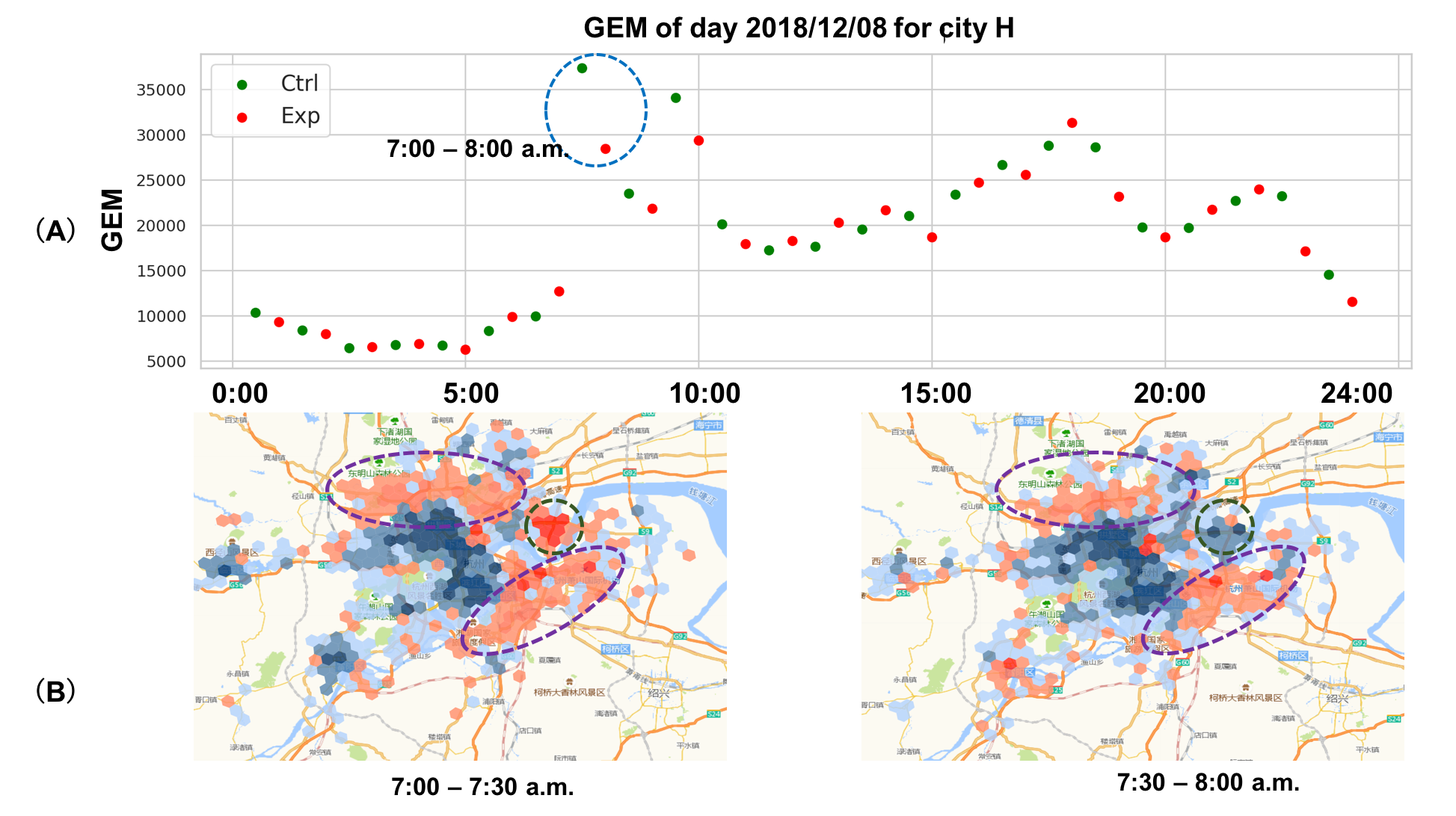
Figure 7: Results from the policy evaluation. (A) The GEM values of a randomly selected day on 2018/12/08 for city H at 30-min scale. Green and red points represent the GEM values generated by the baseline (control) and new (experimental) policies, respectively. In particular, we mark the time period 7:00 to 8:00 a.m. by a blue circle, which demonstrates a significant reduction of GEM value when changing the policy from the the control one to the experimental one. (B) The heatmaps of vertex-wise supply-demand difference $\mbox{DSd}_{it}$ of city H under the control and experimental policies within the 30-min time window from 7:00 to 7:30 am and that from 7:30 to 8:00 am, respectively. Hexagons in red and blue colors represent the locations with positive and negative $\mbox{DSd}_{it}$, respectively, and a deeper color corresponds to a big $|\mbox{DSd}_{it}|$ value.

We conduct an experiment using another supply-demand data set of the same city H from December 3rd to December 16th, 2018 in order to compare the effectiveness between two order dispatching policies. We executed them alternatively on successive half-hourly time intervals. Moreover, we start with the baseline policy being in the first half hour and change the policy every half hour through the whole day and reverse their order in another day. We include an A/A test, which compares the baseline policy against itself, by using the historical data obtained from November 12th to November 25th as a direct comparison. We calculate GEM within each time window of 30 minutes as follows. There are in total $M_{T}=48$ time intervals per day. To obtain GEM in each time interval $\mathcal{T}$, we aggregate 30 GEM values, each of which is calculated within the 1-min timestamp, by using normalization weights $o_{it}/\sum_{t\in\mathcal{T}}\sum_{v_{i}\in\mathbb{V}}o_{it}$.

We first need to introduce some notation. We denote $y_{m}(t_{k})$ as the aggregated GEM value and use $x_{m}(t_{k})$ to denote a $2\times 1$ vector of predictors, which are not strongly influenced by order dispatching policy, including the total number of demands and the total supply time of all drivers in the $k$-th time interval of day $m$ for $k=1,\ldots,M_{T}$ and $m=1,\ldots,M_{D}$. Let $a_{m}(t_{k})=1$ if the new policy is used and $=-1$ otherwise. To examine the marginal effect of policy on GEM, we consider the following regression model:

$$y_{m}(t_{k}) =\beta_{0}(t_{k})+\beta_{1}(t_{k})^{T}\{x_{m}(t_{k})-\overline{x}(t_{k})\}+\beta_{2}(t_{k})a_{m}(t_{k})+\eta_{m}(t_{k})+\varepsilon_{m}(t_{k}),$$ (14)

where $\beta(t_{k})=(\beta_{0}(t_{k}),\beta_{1}(t_{k})^{T},\beta_{2}(t_{k}))^{T}$ is a vector of regression coefficients at $t_{k}$, and $\overline{x}(t_{k})$ is the sample mean of all $x_{i}(t_{k})$s for $k=1,\ldots,M_{T}$. In addition, we assume that $\eta_{m}=(\eta_{m}(t_{1}),\ldots,\eta_{m}(t_{M_{T}}))^{T}$ and $\varepsilon_{m}=(\varepsilon_{m}(t_{1}),\ldots,\varepsilon_{m}(t_{M_{T}}))^{T}$ are $M_{T}\times 1$ vectors of random errors, following mutually independent multivariate Gaussian distributions $N(\textbf{0},\Sigma_{\eta})$ and $N(\textbf{0},\sigma^{2}_{\varepsilon}\cdot{\bf I}_{M_{T}})$, where $\Sigma_{\eta}$ is an $M_{T}\times M_{T}$ matrix and $\sigma^{2}_{\varepsilon}$ is a positive scalar. We are interested in testing the following null and alternative hypotheses:

$$H_{0}:\int_{0}^{M_{T}}\beta_{2}(t)dt=0~{}~{}~{}\mbox{v.s.}~{}~{}H_{1}:\int_{0}^{M_{T}}\beta_{2}(t)dt\not=0,$$ (15)

where $\int_{0}^{M_{T}}\beta_{2}(t)dt\approx\sum_{k=1}^{M_{T}}\beta_{2}(t_{k})\Delta t_{0}$ denotes the average treatment effect per day, in which $\Delta t_{0}$ is the length of each time interval. We propose a joint estimation procedure based on Generalized Estimating Equations (GEE) to iteratively estimate all unknown parameters until a specific convergence criterion being reached (Liang & Zeger, 1986). Subsequently, we compute the $t-$test statistic associated with the average treatment effect per day and its corresponding one-sided (or two-sided) $p-$value (Mancl & DeRouen, 2001).

Furthermore, we consider three global operational metrics including the order answer rates, order finishing rate, and gross merchandise value (GMV) as $y_{m}(t_{k})$ in model (14). We fit the corresponding three regression models in order to study whether the new dispatching policy significantly improves the ride-sourcing platform at the operational level.

Table 4 summarizes all regression analysis results for both the A/A and A/B experimental designs. We can see that in the A/B experimental design, there exists a significant increase in the mean answer rate, finishing rate and gross merchandise value when replacing the old policy by the new one since all the $p-$values associated with the average treatment effect are smaller than $10^{-3}$. The new policy can also significantly reduce the GEM value ($p-$value smaller than $0.05$), which agrees with our assumption that GEM can sufficiently quantify the supply-demand relationship and subsequently affect the examined platform indexes. In contrast, Table 4 shows that in the A/A experimental design, all the four metrics do not show significant treatment effect at the significance level of $5\%$.

Figure 7(A) presents the GEM value at in total 48 30-min time windows on December 3rd, 2018 for the A/B experimental design. We observe a significant reduction of GEM value when changing the policy from the the control one to the experimental one during the time period from 7:00 to 8:00 a.m. Figure 7(B) presents the heat maps of vertex-wise $\mbox{DSd}_{it}$ within the same time period under the control and experimental policies, respectively. The customer requests in three selected regions marked by green and purple circles were satisfied by the drivers in nearby regions, resulting in the higher supply-demand coherence and thus a smaller GEM value.

Table 1: Results from the answer-rate prediction. Comparisons of Hellinger, $L_{2}$-distance, Wasserstein, and GEM in predicting answer rate at $t+10$ and $t+60$ minutes. Peak hour denotes the time from 6 pm to 8 pm. MAPE and RMSE denote the mean absolute percentage error and root mean squared error, respectively.

			Hellinger	L2-distance	Wasserstein	GEM
t+10	All time	RMSE	0.1362	0.1496	0.1273	0.0552
		MAPE	0.0801	0.0891	0.0718	0.0338
	Peak hour	RMSE	0.2219	0.2187	0.2088	0.0614
		MAPE	0.1494	0.1457	0.1089	0.0422
t+60	All time	RMSE	0.1522	0.1552	0.1413	0.1130
		MAPE	0.0828	0.0868	0.0859	0.0620
	Peak hour	RMSE	0.2395	0.2565	0.2222	0.1530
		MAPE	0.1077	0.1159	0.1317	0.0728

Table 2: Results from order dispatching policies. Comparisons of the three policies with respect to two evaluation metrics including the drivers’ revenue and the global answer rate using the simulator for city S on two selected Weekdays. The rows with $(\alpha_{3},\alpha_{4})=(0,0)$ correspond to the first (or baseline) policy, those with $\alpha_{4}=0$ and $\alpha_{3}\not=0$ correspond to the second policy, and all other rows correspond to the third policy. The numbers in the parentheses denote the relative improvement of the corresponding policy over the baseline policy for each evaluation metric.

$\alpha_{3}$	$\alpha_{4}$	Drivers’ Revenue (Yuan)	Order Answer Rate
2018/05/15 (Tuesday)
0	0	1191316	0.737
0.54	0	1227175(+3.01%)	0.760(+3.12%)
0.54	6	1235037(+3.67%)	0.761(+3.28%)
0.54	7	1236824(+3.82%)	0.763(+3.54%)
0.54	8	1240518(+4.13%)	0.765(+3.82%)
0.54	9	1238850(+3.99%)	0.764(+3.66%)
0.54	10	1231702(+3.39%)	0.761(+3.26%)
2018/05/18 (Friday)
0	0	13943666	0.539
0.61	0	14701230(+5.43%)	0.557(+3.34%)
0.61	6	14845486(+6.47%)	0.561(+4.08%)
0.61	7	14858400(+6.56%)	0.560(+3.90%)
0.61	8	14865454(+6.61%)	0.560(+3.90%)
0.61	9	14867573(+6.63%)	0.560(+3.90%)
0.61	10	14823121(+6.31%)	0.557(+3.34%)

Table 3: Results from order dispatching policies. Comparisons of the three policies with respect to two evaluation metrics including the drivers’ revenue and the global answer rate using the simulator for city S on a selected Weekend.

$\alpha_{3}$	$\alpha_{4}$	Drivers’ Revenue (Yuan)	Order Answer Rate
2018/05/19 (Saturday)
0	0	13507568	0.745
0.52	0	13886185(+2.80%)	0.768(+3.09%)
0.52	6	14034453(+3.90%)	0.774(+3.89%)
0.52	7	14008847(+3.71%)	0.772(+3.62%)
0.52	8	14043995(+3.97%)	0.773(+3.76%)
0.52	9	13996021(+3.62%)	0.770(+3.36%)
0.52	10	13934895(+3.16%)	0.768(+3.09%)

Table 4: Results from the policy evaluation: relative improvement and two-sided $p-$value of average treatment effects for the A/A and A/B experiments

Experiment Design	$y_{m}(t)$	Relative Improvement($\%$)	$p-$value
	Answer Rate	0.76	1.16e-12
A/B	Finish Rate	0.36	4.32e-3
	GMV	0.86	2.91e-6
	GEM	-0.80	4.06e-2
	Answer Rate	0.01	0.96
A/A	Finishing Rate	0.01	0.96
	GMV	-0.08	0.72
	GEM	-0.25	0.43

References

- (1)
- Ambrosio & Gangbo (2008) Ambrosio, L. & Gangbo, W. (2008), ‘Hamiltonian odes in the wasserstein space of probability measures’, Communications on Pure and Applied Mathematics: A Journal Issued by the Courant Institute of Mathematical Sciences 61(1), 18–53.
- Arjovsky et al. (2017) Arjovsky, M., Chintala, S. & Bottou, L. (2017), Wasserstein generative adversarial networks, in ‘International Conference on Machine Learning’, pp. 214–223.
- Cha (2007) Cha, S.-H. (2007), ‘Comprehensive survey on distance/similarity measures between probability density functions’, City 1(2), 1.
- Chizat et al. (2018) Chizat, L., Peyré, G., Schmitzer, B. & Vialard, F.-X. (2018), ‘Scaling algorithms for unbalanced optimal transport problems’, Mathematics of Computation 87(314), 2563–2609.
- Dyer et al. (1986) Dyer, M. E., Prieze, A. M. & Mcdiarmid, C. J. H. (1986), ‘On linear programs with random costs’, Mathematical Programing 35, 3–16.
- Grenander & Miller (2007) Grenander, U. & Miller, M. (2007), Pattern Theory From Representation to Inference, Oxford University Press.
- Liang & Zeger (1986) Liang, K.-Y. & Zeger, S. L. (1986), ‘Longitudinal data analysis using generalized linear models’, Biometrika 73(1), 13–22.
- Liao (2003) Liao, Z. (2003), ‘Real-time taxi dispatching using global positioning systems’, Communications of the ACM 46(5), 81–83.
- Liero et al. (2018) Liero, M., Mielke, A. & Savaré, G. (2018), ‘Optimal entropy-transport problems and a new hellinger–kantorovich distance between positive measures’, Inventiones mathematicae 211(3), 969–1117.
- Mancl & DeRouen (2001) Mancl, L. A. & DeRouen, T. A. (2001), ‘A covariance estimator for gee with improved small-sample properties’, Biometrics 57(1), 126–134.
- Munkres (1957) Munkres, J. (1957), ‘Algorithms for the assignment and transportation problems’, Journal of the society for industrial and applied mathematics 5(1), 32–38.
- Piccoli & Rossi (2014) Piccoli, B. & Rossi, F. (2014), ‘Generalized wasserstein distance and its application to transport equations with source’, Archive for Rational Mechanics and Analysis 211(1), 335–358.
- Rabin & Papadakis (2015) Rabin, J. & Papadakis, N. (2015), Convex color image segmentation with optimal transport distances, in ‘International Conference on Scale Space and Variational Methods in Computer Vision’, Springer, pp. 256–269.
- Solomon et al. (2014) Solomon, J., Rustamov, R., Guibas, L. & Butscher, A. (2014), Wasserstein propagation for semi-supervised learning, in ‘International Conference on Machine Learning’, pp. 306–314.
- Steele (1987) Steele, J. M. (1987), Probability Theory and Combinatorial Optimization, Society for Industrial and Applied Mathematics.
- Villani (2008) Villani, C. (2008), Optimal transport: old and new, Vol. 338, Springer Science & Business Media.
- Wang & Yang (2019) Wang, H. & Yang, H. (2019), ‘Ridesourcing systems: A framework and review’, Transportation Research Part B: Methodological 219, 122–155.
- Xu et al. (2018) Xu, Z., Li, Z., Guan, Q., Zhang, D., Li, Q., Nan, J., Liu, C., Bian, W. & Ye, J. (2018), Large-scale order dispatch in on-demand ride-hailing platforms: A learning and planning approach, in ‘Proceedings of the 24th ACM SIGKDD International Conference on Knowledge Discovery & Data Mining’, ACM, pp. 905–913.
- Zhang & Pavone (2016) Zhang, R. & Pavone, M. (2016), ‘Control of robotic mobility-on-demand systems: a queueing-theoretical perspective’, The International Journal of Robotics Research 35(1-3), 186–203.