Fast Classification Learning with Neural Networks and Conceptors for Speech Recognition and Car Driving Maneuvers

Abstract

Recurrent neural networks are a powerful means in diverse applications. We show that, together with so-called conceptors, they also allow fast learning, in contrast to other deep learning methods. In addition, a relatively small number of examples suffices to train neural networks with high accuracy. We demonstrate this with two applications, namely speech recognition and detecting car driving maneuvers. We improve the state of the art by application-specific preparation techniques: For speech recognition, we use mel frequency cepstral coefficients leading to a compact representation of the frequency spectra, and detecting car driving maneuvers can be done without the commonly used polynomial interpolation, as our evaluation suggests.

1 Introduction

The field of artificial intelligence nowadays is dominated by machine learning and big data analysis, in particular with deep neural networkslong [6]. Deep learning in general means a class of machine learning algorithms that use a cascade of multiple layers of nonlinear processing units for feature extraction and transformation [4]. The tremendous success of deep learning in diverse fields of artificial intelligence such as computer vision and natural language processing seems to depend on a bunch of ingredients: deep networks with nonlinearly activated neurons, convolutional layers, and iterative training methods like backpropagation.

Since deep neural networks often consist of thousands of neurons, the corresponding learning procedures require a large number of training examples, usually several thousands per example class for classification tasks (cf., e.g., [29]). Otherwise the networks do not generalize well, and overfitting is a problem. So it would be nice to work with smaller networks, which also reduces the time for training neural networks significantly. For this, we investigate small recurrent neural networks (RNNs) and their applicability to different tasks.

We demonstrate that a relatively small number of examples suffices to train neural networks with high accuracy by two applications, namely speech recognition and detecting car driving maneuvers. We employ RNNs, more precisely echo state networks (ESNs) with conceptors [14, 16, 17]. Training them is very fast, and they can effectively be learned by simply solving a linear equation system, backpropagation or similar methods are not needed. Moreover, we improve the state of the art by application-specific preparation techniques.

2 Background and Related Works

2.1 Recurrent Neural Networks

longRNNs can be used to create temporal dependencies, which occur in many sequence modeling tasks [26]. Nevertheless, RNNs are not the only models capable of representing time dependencies. Hidden Markov models (HMMs), that develop an observed sequence as probabilistically dependent upon a sequence of unobserved states, can be used as well [1]. However, RNNs overcome the main limitation of Markov models by capturing long-range time dependencies [1]. They contain recurrent connections that make them a powerful means to model sequential data [23]. RNNs can maintain an activation even in the absence of input and thus exhibit dynamic memory [18]. A general RNN in contrast to a feed-forward network is shown in Figure 1. The key advantages of RNNs can be seen quickly: Feedback from the output back to the hidden states is possible, as well as recurrent connections in the hidden states itself.

Figure 1: Comparison of the architecture of a feed-forward network (left) with a recurrent neural network (right). The gray arrows show the direction of computation. Feed-forward networks compute only in one direction in contrast to RNNs which have recurrent dependencies (cf. [2]).

We now briefly introduce RNNs, following the lines of [16]. We use discrete-time RNNs where time is progressed in unit steps $n=1,2,\dots$ and $\tanh$ (hyperbolic tangent) as activation function which squashes the neuronal activation values into a range between $-1$ and $+1$. For a network consisting of $N$ neurons, the activations $x_{1}(n),\dots,x_{N}(n)$ at time $n$ are collected in an $N$-dimensional state vector $x(n)$. The long(at least in the beginning) random weights of the neuronlong connections are collected in a weight matrix $W^{\text{res}}$ of size $N\times N$. $p(n)$ is the input signal fed to the network, where the input weights are collected in the weight matrix $W^{\text{in}}$ of size $N\times d$ (for a $d$-dimensional input). $b$ is a bias. The network update equation is:

$$x(n+1)=\tanh\left(W^{\text{res}}x(n)+W^{\text{in}}p(n+1)+b\right)$$ (1)

The network-internal neuron-to-neuron connections comprised in the matrix $W^{\text{res}}$ are (and remain) random. This includes the existence of cyclic (recurrent) connections. The equation

$$y(n)=W^{\text{out}}x(n)$$ (2)

specifies that an output signal $y(n)$ can be read from the network activation state $x(n)$ via the output weights comprised in the matrix $W^{\text{out}}$ of size $d\times N$. These weights $W^{\text{out}}$ are computed by simply solving the linear equation system of Equation 2 such that the output signal $y(n)$ is the prediction of the (next) input signal $p(n)$, i.e., $y(n)=p(n+1)$.

2.2 Echo State Networks and Conceptors

ESNs provide a supervised learning principle for RNNs.long The basic ESN network architecture is shown in Figure 2. They employ a randomly connected neural network with fixed random weights, called reservoir.long In Figure 2 the reservoir coincides with the $N$ internal units with the random fixed weights in $W^{\text{res}}$. Only the connections from the reservoir to the output readout neurons are modified in the training phase by learning [18].long This is possible because of the echo state property. It says that any random initial state of a reservoir is “forgotten” after a washout period such that the current network state is a function of the driver [16]. The input signal of an ESN induces a non-linear response signal in each neuron within the reservoir network. A linear combination of these response signals is trained to obtain the desired output [16, 18]. That is why training an ESN becomes a simple linear regression task [18] (cf. Section 2.1).

long

Figure 2: The basic network architecture of an echo state network (cf. [12]). Dashed arrows indicate connections that are possible but not required.

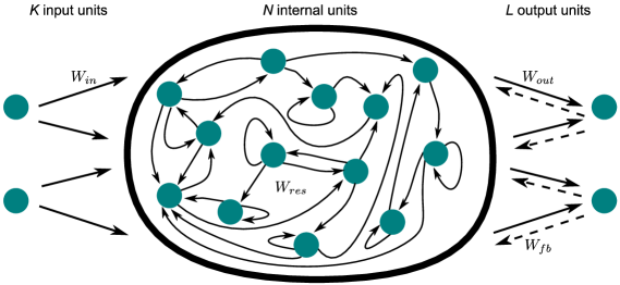
According to [13], ESNs can be generated by the following procedure:

1. Generate a random internal weight matrix $W_{0}$.

2. Normalize $W_{0}$ to a matrix $W_{1}$ with unit spectral radius by putting $W_{1}=1/|\lambda_{\text{max}}|\cdot W_{0}$, where $\lambda_{\text{max}}$ is the spectral radius of $W_{0}$.

3. Scale $W_{1}$ to $W^{\text{res}}=\alpha\cdot W_{1}$, with $\alpha<1$, whereby $W^{\text{res}}$ has a spectral radius of $\alpha$.

4. The untrained network ($W^{\text{in}},W^{\text{res}},W^{\text{out}}$) is then an ESN, regardless of how $W^{\text{in}}$, $W^{\text{out}}$ are chosen.

Conceptors, their basic mechanisms and characteristics and a mathematical definition are described in [\optlongjaeger2014conceptors, 16, 17]. In [16, Sect. 3.13], the classification of Japanese vowels by means of conceptors is considered: Nine male native speakers pronouncing the Japanese di-vowel /ae/ should be recognized. The corresponding procedure employing conceptors has served as the basis for the tasks considered here: speech recognition and car driving maneuvers classification. long[17] focuses on neural long-term memory for temporal patterns. In that paper, conceptors are described more general as a neuro-computational mechanism which can be used in diverse neural information processing tasks like neural noise suppression, stabilization of neural state dynamics and signal separation.

Let us now introduce conceptors in some more detail, following the lines of [16]: A conceptor matrix $C$ for some vector-valued random variable $x\in\mathbb{R}^{N}$ is defined as a linear transformation that minimizes a loss function:

$$C(R,\alpha)=\textnormal{argmin}_{C}\;E\left[\left\|x-Cx\right\|^{2}\right]+\alpha^{-2}\left\|C\right\|^{2}_{\text{fro}}$$ (3)

where $\alpha$ is a control parameter, called aperture, $E$ stands for the expectation value (temporal average), and $||\cdot||_{\text{fro}}$ is the Frobenius norm. The closed-form solution for this optimization problem is

$$C(R,\alpha)=R(R+\alpha^{-2}I)^{-1}=(R+\alpha^{-2}I^{-1})R$$ (4)

where $R=E[xx^{{}^{\prime}}]$ is the $N\times N$ correlation matrix of $x$, and $I$ is the $N\times N$ identity matrix. longNote that the inverses appearing in Equation 4 are well-defined because $\alpha>0$ is assumed, which implies that all singular values of $C(R,\alpha)$ are properly smaller than $1$.

To understand Equation 4, we have to look at the singular value decomposition (SVD) of $C$. If $R=U\Sigma V$ is the SVD of $R$ (where $\Sigma$ is a rectangular diagonal matrix with non-negative real numbers on the diagonal), then the SVD of $C(R,\alpha)$ can be written as $USV$ where the singular values $s_{i}$ of $C$ (comprised in the diagonal matrix $S$) can be written in terms of the singular values $\sigma_{i}$ of $R$: $s_{i}=\sigma_{i}/(\sigma_{i}+\alpha^{-2})\in[0,1)$, for $\alpha\in(0,\infty)$.

[16] finds that the non-linearity inherent in Equation 3 makes the conceptor matrices come out almost as projector matrices because the singular values of $C$ are mostly close to $1$ or $0$. In intuitive terms, $C$ is a soft projection matrix on a linear subspace, where samples $x$ are projected into this subspace. $C$ almost acts like the identity: $Cx\approx x$. longWhen some noise $\xi$ orthogonal to the subspace is added to $x$, $C$ reconstructs $x$ by filtering the noise: $C(x+\xi)\approx x$.

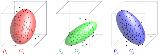
Conceptor matrices are positive semi-definite matrices whose singular vectors are the axes of the conceptor ellipsoids. Their singular values in the unit interval $[0,1]$ represent the lengths of the ellipsoid axes. longThree examples of different patterns with their corresponding conceptor ellipsoids are shown in Figure 3. In practice, the correlation matrix $R$ is estimated from a finite sample $X=(x(1),\dots,x(L))$ where the $x(n)$ are the reservoir states collected during a learning run. This leads to the approximation $R_{\text{approx}}=XX^{T}/L$. An optimal aperture $\alpha$, which can be interpreted as a scaling factor, can be found by a cross-validation search (cf. [8]). Using the correlation matrix $R_{j}$ from a pattern $p_{j}$ and $\alpha$, one can compute the conceptor matrix $C^{j}=C(R_{j},\alpha)$.

long

Figure 3: Conceptors $C^{1},C^{2},C^{3}$ of three pattern $p^{1},p^{2},p^{3}$ of a network with $N=3$ reservoir neurons.

3 Classification with Conceptors

3.1 Conceptor Algebra

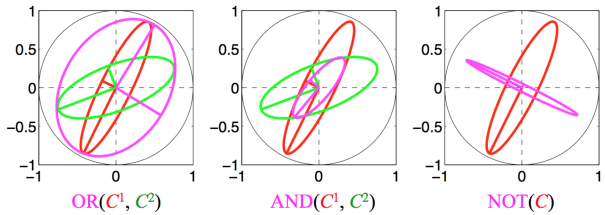
On matrix conceptors, operations that satisfy most laws of Boolean logic such as NOT ($\lnot$), OR ($\lor$), and AND ($\land$) can be defined [8]long, as shown in Figure 4. Although not all laws of Boolean algebra are satisfied, these operations bring a great advantage for conceptors, because if we get new patterns we need not train everything from the start, but use overlaps with other already saved patterns and just save the new components (which saves memory space) [16]. Furthermore, we can use Boolean operations to check how many patterns lie in one conceptor and not in any other and for similar considerations.

long

Figure 4: Boolean operations on 2-dimensional conceptors are shown (cf. [8]). Red/green ellipses represent source conceptors $C^{1}$, $C^{2}$ and the pink ellipses show $C^{1}\lor C^{2}$, $C^{1}\land C^{2}$, $\lnot C^{1}$ from left to right.

3.2 Classification

To use conceptors for a classification task, we first determine two conceptors, called positive and negative evidence, for each class, e.g., words, speakers, or car driving maneuvers, based on the training data. For instance, for the classification of nine speakers, we have twice as many conceptors. For every class, we compute (train) one conceptor $C^{j}$ characteristic of class $j$ and determine a second conceptor

$$N^{j}=\lnot(C^{1}\lor\dots\lor C^{j-1}\lor C^{j+1}\lor\dots\lor C^{m})$$ (5)

where $\lnot$ is the Boolean negation (NOT), $\lor$ is the Boolean operation disjunction (OR) and $m$ is the number of different classes. This characterizes the condition that this class $j$ is not any of the other classes $1,\dots,j-1,j+1,\dots,m$.

After the training phase, we can classify a sample by computing the evidence values for each conceptor as well as a combined evidence. The class corresponding to the conceptor with the highest evidence value is then assumed to be the correct classification. We get the positive evidence of a conceptor by computing $E^{+}(p,j)=x^{T}C^{j}x$ where $x$ is the response signal of the network. This leads to a classification by deciding for $j=\text{argmax}_{i}\,x^{T}C^{+}_{i}x$ to select class $j$. $E^{+}(p,j)$ is a non-negative number indicating how well the signal fits into the ellipsoid of $C^{j}$. The idea behind this is that, if the reservoir is driven by a class $j$, the resulting response signal $x$ will be located in a linear subspace of the (transformed) reservoir state space whose overlap with the ellipsoids $C_{i}$ $(i=1,\dots,m)$ is maximal for $i=j$.

Similarly, the negative evidence $E^{-}(p,j)=x^{T}N^{j}x$ (which has a positive value despite its name) is computed. It describes that the sample $p$ is of class j and not one of the other classes. Since $E^{-}(p,j)=x^{T}N^{j}x$ we can compute the negative evidence of a pattern using the Boolean operations NOT and OR (cf. Equation 5). To obtain the combined evidence, we simply sum up the previous two values:

$$E(p,j)=E^{+}(p,i)+E^{-}(p,i)$$ (6)

Thus the combined evidence has a greater value if both the positive evidence $E^{+}(p,j)$ and the negative evidence $E^{-}(p,j)$ have high values. This is the case if the signal is inside the conceptor $C^{j}$ and has low overlap with any other conceptor. For each utterance, we compute $m$ combined evidences $E(p,1),\dots,E(p,m)$. The pattern $p$ can then be classified as class $j$ by choosing the class index $j$ whose combined evidence $E(p,j)$ was the greatest among the collected evidences.

4 Case Studies

4.1 Speech Recognition

In this case study, we consider two different tasks: A. recognition of isolated words and B. speaker recognition. We used speech samples of adults and children of age between $3$ and $45$ years, female and male. The datasets for both tasks overlap but are not identical.

Isolated Word Recognition:

For the recognition of isolated words we have a total of 1320 samples, divided in a training set of 880 utterances (2/3 of all samples) and a test set of 440 utterances (1/3 of all samples). In this task we recognize the German isolated words “halt”, “langsamer”, “links”, “rechts”, “schneller”, “stopp”, “vor”, and “zurück” pronounced by different speakers (adults and children, female and male). For each of our 8 different words we have 110 training and 55 test samples.

Speaker Recognition:

For this task, nine persons spoke different distinct isolated German words (per speaker we used up to 26 different words). The number of speech samples differs per speaker. The training set of every speaker is the same with 65 samples. The amount of test samples varies per speaker. Overall we have 296 test samples. We choose samples of children and adults, female and male speakers to create a diverse dataset, with different speech rate and pronunciation.

The raw speech samples need to be preprocessed, before we can pass them to the neural network. Speech recognition performance and sensitivity depends heavily on preprocessinglong [10, 25], because the amount of data supplied to the input of the neural network usually is reduced by this. Preprocessing differentiates the voiced or unvoiced signal and creates feature vectors [10]. We develop a speaker and isolated word recognition system based on the Japanese vowels classification system in [16] and employ the Matlab code from http://minds.jacobs-university.de/research/conceptorresearch/.

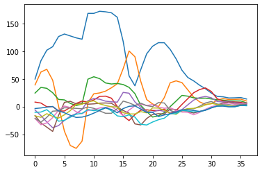
We apply application-specific preparation techniques and divide the signal into discrete sequences of feature vectors that only contain relevant information about the utterance. For this, we extract features by employing mel frequency cepstral coefficients (MFCCs) and obtain uncorrelated vectors by means of discrete cosine transforms (DCT). MFCCs are the most used spectral feature extraction method [5]. It is based on frequency analysis using the mel scale similar to the human ear scale. The coefficients are a representation of the real cepstral of a windowed short-time signal derived from the fast Fourier transform (FFT) of that signal, more precisely, the logarithm of the spectral amplitudes.long The FFT algorithm extracts frequency amplitudes for discrete intervals from a given segment of a signal [7]. Examples of the MFCCs of two different German words are shown in Figure 5. In our experiments, we use 12 MFCCs and thus obtain $12$-dimensional time series by means of a Python implementation using the librosa package for music and audio analysis (see http://librosa.org/). Each utterance is sampled with $512$ data points. Since the length of the original audio files is between $0.6$ and $2.0$ s, the sampling rate is hence between $256.0$ and $853.3$ Hz.

long

(a) “halt”

(b) “langsamer”

Figure 5: Selection of examples of the MFCCs from signals of the two German words “halt” and “langsamer”. From each utterance, we get a $12$-dimensional time series consisting of $12$ MFCCs. The $x$-axis of the plot corresponds to the sampling time steps (one frame consists of $512$ sampling points), and the $y$-axis to the MFCC values. As the exemplary utterances are from kids, which tend to have higher frequencies, the MFCC values are relatively high.

4.2 Car Driving Maneuvers

In this case study, we investigate whether driving maneuvers can be classified by the use of conceptors. Driving behavior has already been analyzed in several papers, and possible applications have been presented [9, 11, \optlongjohnson2011, 24, 27, vaiana2014\optlong, 30]. We investigate here whether conceptors can also be used for car driving maneuver detection. Furthermore, we consider the influence of the number of reservoir neurons and whether very small training datasets are sufficient to train a conceptor.

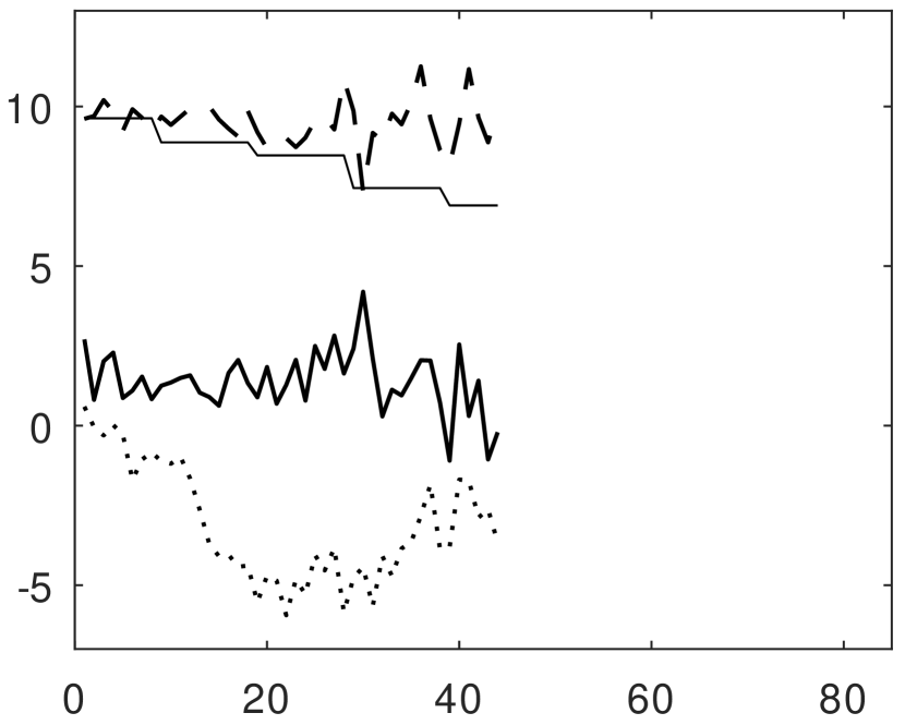
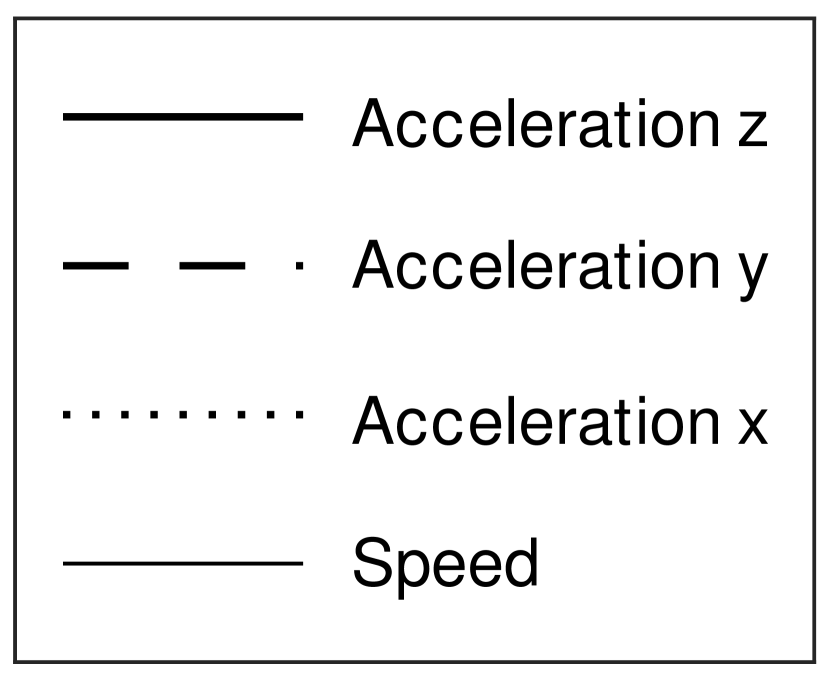
The classification method we used for this task is based on the dynamic pattern recognition method in [16, p. 74]. In addition, we have investigated whether all components of the classification method in [16] are actually necessary for the car driving maneuver classification task (cf. Section 5.3). The data was recorded with a smartphone which was permanently installed in the car while driving. We took care of a fix position of the smartphone relative to the vehicle. An app (written by the second author, cf. [21]) continuously recorded the lateral, longitudinal, and gravitational acceleration acting on the vehicle as well as the GPS data. The speed was derived from the GPS data. The sampling rate was $10$ Hz.

Table 1: Overview of car driving maneuvers.

class index $j$	maneuvers	number of samples
1	stop	10
2	straight ahead	9
3	start up	11
4	slow down	8
5	full braking	8
6	left turn	15
7	right turn	17

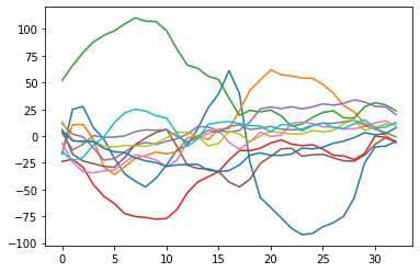
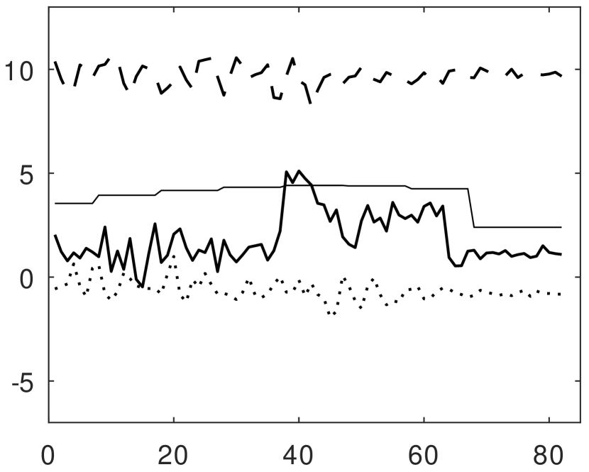
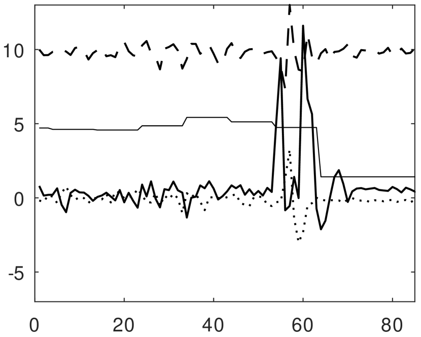
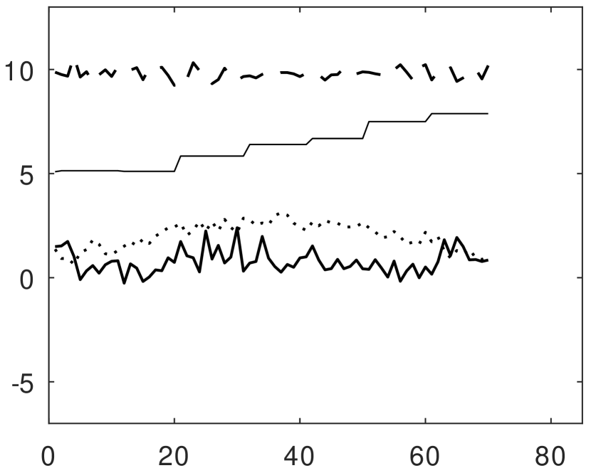
This test setup was used to collect the required data for seven different maneuvers. The types of car driving maneuvers and number of measurement series used for classification are shown in Table 1. For the classification task, only those sections of the measurement series were used whose features were typical for the car driving maneuver in question. This gives us the ground truth of the data. Typical measurement series are shown in Figure 6. For the classification task, initially only the training data was classified. For each class $j$, the conceptors for the classification were calculated with $8$ measurement series. The number of reservoir neurons $N$ was varied between $2$ and $60$, and for $N=10$ the number of training examples was varied. longIn these analyses, the available datasets were divided into a training set and a test set. At the same time, the number of measurement series used for training varied such that 7 conceptors $C_{j}^{+}$ and $C_{j}^{-}$ were calculated for each class $j$. The smallest training set always consisted of two samples and was gradually increased until the training set finally consisted of eight samples.

(a) slow down

(b) full braking

long

(c) right turn

(d) left turn

Figure 6: Selection of examples of typical maneuver samples (acceleration in $\text{m}/\text{s}^{2}$ and velocity in $\text{m}/\text{s}$). Note that, following the lines of [16], we used only $4$ states (called support points) for the conceptor calculation from all measurement series.

5 Evaluation

longIn this section, we present the results of our isolated word and speaker recognition task as well as the evaluation of the car driving maneuvers.

5.1 Speech Recognition

In both speech recognition tasks, we used 50 random ESNs to compare our results. Task A (word recognition) was to classify eight different German words. For each class of words, a positive and a negative conceptor is created (cf. Section 3.2). With them, we calculate the combined evidence (cf. Equation 6) to classify test samples. We use the combined evidence classification, because its accuracy is higher in comparison to the positive or negative evidence classification alone. In Table 3, the error rates of Task A with and without conceptors as well as the error rate of a random guess are compared. With conceptors, our speech recognition system works nearly two times better than an ESN without conceptors. In addition, our method (with conceptors) is about 2.4 times better than a random guess, even if the samples of each class are not that similar.

The goal in Task B (speaker recognition) was to classify nine speakers. Without conceptors, we have a mean of 161 false classifications in 50 trials, which equals a mean error rate of 0.544. This misclassification rate is 3.5 times higher than the mean error rate of the same task with the use of conceptors. Our error rate of 0.155 with conceptors in Task B is much smaller than in Task A. The reason probably is that, in Task A, female and male speakers have different fundamental voice frequencies pronouncing the same isolated word. Therefore an analysis that is more invariant to voice frequencies would be desirable.

Table 2: Error rates of our two tasks: A. word recognition and B. speaker recognition.

error rates	Task A	Task B
with conceptors	0.366	0.155
without conceptors	0.711	0.544
random guess	0.875	0.889

Table 3: Program runtimes for Task A and Task B.

runtime [s]	Task A	Task B
training	0.1704	0.1396
test	0.0057	0.0066

To compare our results with similar speaker recognition tasks using conceptors, we investigate the speaker classification task in [16] where it is tried to recognize nine male speakers pronouncing the Japanese di-vowel /ae/. Our dataset is more diverse in contrast to this dataset, because we use samples of female and male speakers of different ages. We assume that is the reason why the mean error rate (combined evidence) 0.062 with the dataset of [16] is better than the rate of 0.155 for our dataset. We have to be careful directly comparing the error rates, however, because [16] uses linear predictive coding (LPC) cepstrum coefficients for data preprocessing, whereas we use MFCCs. Note that it is not our goal to improve the state-of-the-art word error rate. We aim to show that we already get good results with a small dataset within very short training time using ESNs and conceptors. longIf the reader is interested in an accurate automatic speech recognition software for German words take a look at [20], where 412 training hours for 510 speakers have been spent.

In Table 3, it is shown that the two experiments deliver fast in training and testing. Our Matlab implementation needs less than $1$ s for the training from over 500 samples. This is due to the fact that we used ESNs where the majority of the weights in the network need not be trained. In comparison to other neural networks, like convolutional neural networks (CNNs)long (cf. [6]) which need thousands of samples and a long training time to get good results, our study yields proper results already with limited training. Note that the reported accuracy of CNNs with error rates less than 1% eventually is higher. Since the error rate should be low in most speech recognition tasks, a direct comparison of the proportion of misclassifications with the results of the presented tasks would be necessary (with consideration of the dataset and used classification method). Nonetheless, we find using conceptors in both tasks reduces our error rate many times. This makes conceptors a very powerful means to improve speech recognition tasks, which should be tested and verified further, of course.

5.2 Car Driving Maneuvers

In this section, we describe our findings with which reservoir size and which amount of training data classification of car driving maneuvers is possible. Section 5.2 shows the results of classifications with different reservoir sizes. For each class of car driving maneuvers, $h^{+}$ and $h^{-}$ are the positive and negative evidence vectors used for classification [16, p. 77] (cf. Section 3.2). One aim was to find out whether the reservoir size has a significant influence on the classification. The smallest reservoir we used had 2 neurons, the largest 60 neurons. For each reservoir size, 100 random reservoirs were generated. The conceptors of positive and negative evidence (cf. Section 3.2) were calculated for each driving maneuver and each reservoir. For each driving maneuver and reservoir, eight measurement series have been used to calculate the conceptors.

As it can be seen in Section 5.2, our experiments allow classification with very small reservoirs. In the first five classes, two neurons are sufficient for an almost 100% correct classification. Only for the driving maneuvers “straight ahead” and “full braking”, the correctness is only 36% and 31% respectively. But the classification accuracy could be improved with larger reservoirs. With the exception of “full braking”, every maneuver is classified correctly with at least 99%. In the case of emergency braking, we assume that significant features of the class are lost due to the previous data processing. Further investigations with alternative support points (cf. Figure 6) optimized for the class of emergency braking finally allow significantly better classifications.

Table 4: Classification of training data. The table shows the accuracy of the computed conceptors for positive and negative evidence in %.

		size of reservoir $N$
Maneuver		2	4	6	8	10	20	30	40	60
start up	$h^{+}$	99.9	100	100	99.9	100	100	99.9	100	100
	$h^{-}$	2.9	11.1	38.4	50.1	51.0	60.1	69.5	79.6	82.0
slow down	$h^{+}$	99.9	99.8	99.3	98.8	99.3	99.6	99.8	99.9	100
	$h^{-}$	1.0	10.8	38.6	39.6	41.3	39.1	41.5	44.1	49.4
right turn	$h^{+}$	99.8	99.9	99.3	98.9	98.0	98.4	96.5	96.1	95.5
	$h^{-}$	78.4	92.6	97.9	98.0	96.4	100	100	100	100
left turn	$h^{+}$	98.5	98.1	97.5	97.8	96.8	99.3	98.9	99.3	99.8
	$h^{-}$	36.1	36.9	79.4	92.6	93.9	98.0	100	100	100
longstop	$h^{+}$	100	100	100	100	100	100	100	100	100
	$h^{-}$	51.6	29.0	79.0	94.0	94.0	98.0	100	100	100

straight ahead & $h^{+}$ 36.1 62.4 89.3 93.0 99.4 100 100 100 100 $h^{-}$ 0.0 0.0 0.0 0.0 0.0 0.0 0.0 0.0 0.0 full braking $h^{+}$ 31.0 34.3 40.4 45.3 47.1 54.4 59.5 60.8 64.3 $h^{-}$ 0.0 0.0 0.0 0.0 0.0 0.0 0.0 0.0 0.0

Section 5.2 (left part) shows the results for classifications with different amounts of training data. For each driving maneuver, a minimum of two measurements series was used to calculate the conceptors. The number of measurement series for the training amount was then gradually increased to eight measurement series. 100 random reservoirs were generated and corresponding conceptors were calculated for each class. This time both the training data and the test data were classified. Since only a small number of measurement series was available, measurement series that were not used for training were automatically assigned to the test set.

Classifications with an accuracy of at least 70.7% and up to 100% could be achieved even with a very small amount of training, consisting of two measurement series. However, again the driving maneuvers “straight ahead” and “full braking” are an exception and are poorly classified. Nevertheless, Section 5.2 (left part) also shows that with increasing training size the accuracy of the classification improves significantly in many cases.

In summary, the accuracy of our car driving maneuver classification is rather good. Using random guessing as baseline, the accuracy of classifying seven different car driving maneuvers would reduce to $1/7=14.3$% which is far less than our values. Furthermore, in other experiments, often only the simpler task of binary classification is considered, e.g., only with respect to driver inattendance [11, 27]. In our experiments, we also investigated open-set testing, i.e., considering also the case that the car driving behavior does not correspond to one of the given maneuvers. For this, the thresholds for the components of the evidence vectors have to be adjusted correctly (see also [21, Sect. 5.2]).

Table 5: Classification with a varying amount of training data (left part) and Comparison of the modifications (right part). Both with a constant reservoir size of $N=10$ neurons. For each driving maneuver, the number of test series $m$ of the test quantity is listed in the line “test”. The number of training series $n$ is listed at the top of the table.

& training $h^{+}$ 93.5 95.7 99.5 95.0 97.7 96.6 95.6 0.6 2.9 -2.6 -1.9 -2.0 3.8 $h^{-}$ 0 0 0 0 0 0 0 0 0 0 0 0 0 test m 7 6 5 4 3 2 1 4 1 4 1 4 1 $h^{+}$ 45.4 74.3 89.6 82.3 80.0 74.5 48.0 2.0 7.0 -4.3 -5.0 -2.3 8.0 $h^{-}$ 0 0 0 0 0 0 0 0 0 0 0 0 0 full braking training $h^{+}$ 87.0 63.0 30.8 34.2 32.8 40.0 46.3 -1.4 1.5 0.8 -2.1 -1.6 0.6 $h^{-}$ 22.0 2.3 0 0 0 0 0 -0.2 0 0 0 0 0 test m 6 5 4 3 2 1 0 3 0 3 0 3 0 $h^{+}$ 11.0 35.6 20.3 36.7 78.5 69.0 - 0.7 - 3.3 - 4.7 - $h^{-}$ 0 0 0 0 0 0 - 0 - 0 - 0 -

long

5.3 Identifying Essential Factors

Let us finally analyze essential factors of car driving maneuver detection, namely the influence of 1. using a linear activation function and 2. omitting polynomial interpolation, which are part of the method in [16], on the classification accuracy:

linear vs. nonlinear activation function:

Motivated by linear neural networks [26] where all neurons are linearly activated, experiments with linear activation were carried out. Only the activation function of the existing classifier was changed for these analyses. Instead of $\tanh$, a linear activation function is applied.

with vs. without polynomial interpolation:

We have analyzed the influence of polynomial interpolation on the classifications of driving maneuvers. For this purpose, polynomial interpolation was not performed after data normalization. Here again $\tanh$ was used as the activation function in these analyses.

In total, $100$ test runs (each with a randomly generated reservoir) with $n=5$ and $n=8$ training data sequences were performed. In Section 5.2 (right part), $h^{+}$ and $h^{-}$ again are the positive and negative evidence vectors used for classification (cf. Section 5.2). We can see how much the classification with linear activation is better or worse than the classification with $\tanh$ as activation function. In the column “polynomial” it is shown how much the classification is better or worse if polynomial interpolation is not performed. The last column shows the results if both linear activation and no polynomial interpolation is performed. Results for the classification of training data and test data are presented separately for each car driving maneuver. The difference between the classification of the original implementation (with polynomial interpolation and the modified implementation) is given in percent. The calculation rule is: $\Delta_{\text{quality}}=\text{quality}_{\text{original}}-\text{quality}_{\text{modification}}$. If $\Delta_{\text{quality}}$ is negative, the classification of the original implementation is worse. These values are highlighted in Section 5.2 (right part).

Looking at the classification of the training measurement series, the classification with linear activation is 2.9% worse in the worst case (“straight ahead”, $h^{+}$, $n=8$). For emergency braking ($h^{+}$, $n=5$) even better by 1.4%. For $h^{-}$ there are also opposing values. For “start up”, the linear activation achieves a better classification (4.0% or 6.8% better), whereas for “slow down” it achieves a significantly worse classification (23.2% or 29.0% worse). Finally, when classifying the training set with a linear activation for $h^{+}$ almost always the same quality is achieved as by the original implementation with $\tanh$.

Polynomial interpolation seems to have less impact on the classification. Although there are again classifications that achieve a worse quality without polynomial interpolation. Overall the quality of the modification is up to 5% better. The greatest (positive) deterioration compared to the original implementation is 4.9% for the “slow down” class (training measurement series, $h^{-}$, $n=8$). Often even the same quality is achieved ($\Delta_{\text{quality}}=0$). For further details the reader is referred to [21].

In conclusion, it should be noted that no uniform result could be achieved, thus a generally positive or negative effect can not be shown. The original and the modified implementations achieve similar quality. But from this we may conclude that the commonly used hyperbolic tangent function and polynomial interpolation is not really mandatory to solve classification tasks. Hence the procedure in [16] can be simplified significantly by using plain linear activation and omitting polynomial interpolation.

6 Conclusions

We have shown that fast learning with ESNs and conceptors is possible for diverse applications, in particular, speech recognition and detecting car driving maneuvers. With already hardly more than one hundred samples per class accurate classification is possible, in contrast to other neural networks like CNNs that require thousands of samples for each class. In addition, training conceptor networks for classification lasts only a few seconds. Nevertheless only with application-specific methods high accuracy is reachable, e.g., using MFCCs for speech recognition. Furthermore, existing procedures can be simplified, e.g., employing simple linear activation and omitting polynomial interpolation without loosing much accuracy, as done for car driving maneuver detection. Further work will consider even more applications and simplifications of RNNs (cf. [26]) and focus more on open-set testing, which seems to be important also for speech recognition [3]. While we use a common one-vs-all classification scheme with as many output units as there are classes in a dataset, a novel one-vs-one classification scheme that trains each output unit to distinguish between a specific pair of classes had recently been developed [22]. A comparison to our classification method could be of further interest.

References

- [1] Al-Smadi, M., Qawasmeh, O., Al-Ayyoub, M., Jararweh, Y., Gupta, B.: Deep recurrent neural network vs. support vector machine for aspect-based sentiment analysis of arabic hotels’ reviews. Journal of Computational Science 27, 386–393 (2018), http://doi.org/10.1016/j.jocs.2017.11.006
- [2] Burgsteiner, H., Kröll, M., Leopold, A., Steinbauer, G.: Movement prediction from real-world images using a liquid state machine. Applied Intelligence 26(2), 99–109 (2007), http://link.springer.com/article/10.1007/s10489-006-0007-1
- [3] Clopper, C.G., Pisoni, D.B., Tierney, A.T.: Effects of open-set and closed-set task demands on spoken word recognition. Journal of the American Academy of Audiology 17(5), 331–349 (2006), http://www.ncbi.nlm.nih.gov/pmc/articles/PMC3324094/
- [4] Deng, L., Yu, D.: Deep learning: Methods and applications. Foundations and Trends in Signal Processing 7(3-4), 198–387 (2014), http://research.microsoft.com/pubs/209355/DeepLearning-NowPublishing-Vol7-SIG-039.pdf
- [5] Dey, N.: Intelligent Speech Signal Processing. Academic Press (2019), http://www.elsevier.com/books/intelligent-speech-signal-processing/dey/978-0-12-818130-0
- [6] Goodfellow, I., Bengio, Y., Courville, A.: Deep Learning. Adaptive Computation and Machine Learning, MIT Press, Cambridge, MA, London (2016), http://www.deeplearningbook.org
- [7] Grewal, S.S., Kumar, D.: Isolated word recognition system for English language. International Journal of Information Technology and Knowledge Management 2(2), 447–450 (2010), http://www.csjournals.com/IJITKM/PDF%203-1/54.pdf
- [8] He, X., Jaeger, H.: Overcoming catastrophic interference using conceptor-aided backpropagation. In: ICLR 2018 – 6th International Conference on Learning Representations. Vancouver (2018), http://arxiv.org/abs/1707.04853
- [9] Hong, J.H., Margines, B., Dey, A.K.: A smartphone-based sensing platform to model aggressive driving behaviors. In: Proceedings of the SIGCHI Conference on Human Factors in Computing Systems. pp. 4047–4056. CHI ’14, ACM, New York, NY, USA (2014), http://doi.acm.org/10.1145/2556288.2557321
- [10] Ibrahim, Y.A., Odiketa, J.C., Ibiyemi, T.S.: Preprocessing technique in automatic speech recognition for human computer interaction: An overview. Annals. Computer Science Series 15(1) (2017), http://anale-informatica.tibiscus.ro/download/lucrari/15-1-23-Ibrahim.pdf
- [11] Islinger, T., Köhler, T., Ludwig, B.: Driver distraction analysis based on FFT of steering wheel angle. In: Adjunct Proceedings of the 3rd International Conference on Automotive User Interfaces and Interactive Vehicular Applications. pp. 21–22 (2011), http://www.auto-ui.org/11/docs/AUI2011˙adjunctproceedings.pdf
- [12] Jaeger, H.: The ”echo state” approach to analysing and training recurrent neural networks – with an erratum note. Tech. Rep. 148, German National Research Center for Information Technology, Bonn, Germany (2001), http://www.ai.rug.nl/minds/uploads/EchoStatesTechRep.pdf, latest revision 2010
- [13] Jaeger, H.: Tutorial on training recurrent neural networks, covering BPPT, RTRL, EKF and the ”echo state network” approach. Tech. Rep. 159, German National Research Center for Information Technology, Bonn, Germany (2002), http://www.cse.iitk.ac.in/users/hk/cs671/201617/details/rnnTutorialJaeger.pdf, latest revision 2013
- [14] Jaeger, H.: Echo state network. Scholarpedia 2(9), 2330 (2007), http://doi.org/10.4249/scholarpedia.2330, revision #151757
- [15] Jaeger, H.: Conceptors: an easy introduction. CoRR – computing research repository, Cornell University Library (2014), http://arxiv.org/abs/1406.2671
- [16] Jaeger, H.: Controlling recurrent neural networks by conceptors. CoRR – computing research repository, Cornell University Library (2014), http://arxiv.org/abs/1403.3369
- [17] Jaeger, H.: Using conceptors to manage neural long-term memories for temporal patterns. Journal of Machine Learning Research 18(1), 387–429 (2017), http://dl.acm.org/doi/abs/10.5555/3122009.3122022
- [18] Jaeger, H., Haas, H.: Harnessing nonlinearity: Predicting chaotic systems and saving energy in wireless communication. Science 304(5667), 78–80 (2004), http://doi.org/10.1126/science.1091277
- [19] Johnson, D.A., Trivedi, M.M.: Driving style recognition using a smartphone as a sensor platform. In: 2011 14th International IEEE Conference on Intelligent Transportation Systems (ITSC). pp. 1609–1615 (Oct 2011), http://doi.org/10.1109/ITSC.2011.6083078
- [20] Milde, B., Köhn, A.: Open source automatic speech recognition for German. In: Proceedings of 13th ITG Conference on Speech Communication, Oldenburg. Universität Hamburg (2018), http://edoc.sub.uni-hamburg.de/informatik/volltexte/2018/243/
- [21] Otto, O.: Analysis of smartphone sensor data with recurrent neural networks for classification of driving maneuvers. WAIT\optlong – Wernigeröder Automatisierungs- und Informatiktexte 03/2020, Automation and Computer Sciences Department, Harz University of Applied Sciences (2020), http://doi.org/10.25673/35931, in German
- [22] Pawara, P., Okafor, E., Groefsema, M., He, S., Schomaker, L.R., Wiering, M.A.: One-vs-one classification for deep neural networks. Pattern Recognition 108, 107528 (2020), http://doi.org/10.1016/j.patcog.2020.107528
- [23] Sak, H., Senior, A.W., Beaufays, F.: Long short-term memory recurrent neural network architectures for large scale acoustic modeling (2014), http://research.google/pubs/pub43905.pdf
- [24] Schüttke, T., Gillmeier, K., Diederichs, F., Spath, D.: Detection of driver distraction based on driving data, interior camera and a capacitive steering wheel. In: Bargende, M., Reuss, H.C., Wiedemann, J. (eds.) 17. Internationales Stuttgarter Symposium. pp. 1133–1148. Springer, Wiesbaden (2017), http://doi.org/10.1007/978-3-658-16988-6˙86
- [25] Shanthi, T.S., Lingam, C.: Review of feature extraction techniques in automatic speech recognition. International Journal of Scientific Engineering and Technology 2(6), 479–484 (2013), http://www.ijset.com/publication/v2/084.pdf
- [26] Stolzenburg, F., Litz, S., Michael, O., Obst, O.: The power of linear recurrent neural networks. CoRR – computing research repository, Cornell University Library (2018), http://arxiv.org/abs/1802.03308, latest revision 2021
- [27] Torkkola, K., Massey, N., Wood, C.: Driver inattention detection through intelligent analysis of readily available sensors. In: Proceedings of 7th International IEEE Conference on Intelligent Transportation Systems (IEEE Cat. No.04TH8749). pp. 326–331 (2004), http://doi.org/10.1109/ITSC.2004.1398919
- [28] Vaiana, R., Iuele, T., Astarita, V., Caruso, M.V., Tassitani, A., Zaffino, C., Giofré, V.: Driving behavior and traffic safety: An acceleration-based safety evaluation procedure for smartphones. Modern Applied Science 8(1), 88–96 (2014), http://doi.org/10.5539/mas.v8n1p88
- [29] Warden, P.: Speech commands: A dataset for limited-vocabulary speech recognition. CoRR – computing research repository, Cornell University Library (2018), http://arxiv.org/abs/1804.03209
- [30] You, C.W., Montes-de Oca, M., Bao, T.J., Lane, N.D., Lu, H., Cardone, G., Torresani, L., Campbell, A.T.: Carsafe: A driver safety app that detects dangerous driving behavior using dual-cameras on smartphones. In: Proceedings of the 2012 ACM Conference on Ubiquitous Computing. pp. 671–672. UbiComp ’12, ACM, New York, NY, USA (2012), http://dx.doi.acm.org/10.1145/2370216.2370360