Random hyperbolic surfaces of large genus have first eigenvalues greater than $\frac{3}{16}-\epsilon$

Abstract.

Let $\mathcal{M}_{g}$ be the moduli space of hyperbolic surfaces of genus $g$ endowed with the Weil-Petersson metric. In this paper, we show that for any $\epsilon>0$, as genus $g$ goes to infinity, a generic surface $X\in\mathcal{M}_{g}$ satisfies that the first eigenvalue $\lambda_{1}(X)>\frac{3}{16}-\epsilon$. As an application, we also show that a generic surface $X\in\mathcal{M}_{g}$ satisfies that the diameter $\operatorname{diam}(X)<(4+\epsilon)\ln(g)$ for large genus.

1. Introduction

Let $X_{g}$ be a hyperbolic surface of genus $g\geq 2$ and $\lambda_{1}(X_{g})$ be the first eigenvalue of the Laplacian operator on $X_{g}$. For large genus, it is known (e.g. see [Hub74] or [Che75]) that

$$\limsup\limits_{g\to\infty}\lambda_{1}(X_{g})\leq\frac{1}{4}$$

for any sequence of hyperbolic surfaces $\{X_{g}\}_{g\geq 2}$. The motivation of this work is whether random objects have large, or even optimal, first eigenvalues. Brooks and Makover in [BM04] showed that there exists a uniform positive lower bound for the first eigenvalues of random surfaces in their discrete model by gluing ideal hyperbolic triangles. In this work we view the first eigenvalue as a random variable with respect to the probability measure $\mathop{\rm Prob}\nolimits_{\rm WP}^{g}$ on moduli pace $\mathcal{M}_{g}$ of Riemann surfaces of genus $g$ given by the Weil-Petersson metric, which was initiated by Mirzakhani in [Mir13]. Based on her celebrated thesis works [Mir07a, Mir07b], Mirzakhani proved the following result via the Cheeger inequality by showing [Mir13, Theorem 4.8] that the Cheeger constant of a generic surface $X\in\mathcal{M}_{g}$ is greater than or equal to $\frac{\ln(2)}{2\pi+\ln(2)}$ as $g$ tends to infinity. More precisely, she showed that

$$\lim\limits_{g\to\infty}\mathop{\rm Prob}\nolimits_{\rm WP}^{g}\left(X\in\mathcal{M}_{g};\ \lambda_{1}(X)\geq\frac{1}{4}\left(\frac{\ln(2)}{2\pi+\ln(2)}\right)^{2}\sim 0.00247\right)=1.$$

The main result of this paper is the following.

Theorem 1.

For any $\epsilon>0$, we have

$$\lim\limits_{g\to\infty}\mathop{\rm Prob}\nolimits_{\rm WP}^{g}\left(X\in\mathcal{M}_{g};\ \lambda_{1}(X)>\frac{3}{16}-\epsilon\right)=1.$$

It is unknown whether Theorem 1 also holds with $\frac{3}{16}$ replaced by $\frac{1}{4}$ (e.g. see [Wri20, Problem 10.4]). We remark here that it is very recently proved by Hide and Magee [HM21] that there exists a sequence of hyperbolic surfaces $\{X_{g_{n}}\}$ with genus $g_{n}$ going to infinity such that $\lambda_{1}(X_{g_{n}})$ tends to $\frac{1}{4}$ (e.g. see [BBD88], [Mon15, Conjecture 1.2], [WX21, Conjecture 5] and [Wri20, Problem 10.3]).

Remark.

Mysteriously,

1. the number $\frac{3}{16}$ is the lower bound in a celebrated theorem of Selberg [Sel65] saying that congruence covers of the moduli surface $\mathbb{H}/\rm{SL(2,\mathbb{Z})}$ have first eigenvalues $\geq\frac{3}{16}$. Meanwhile in [Sel65] the Selberg eigenvalue conjecture was also proposed, which asserts that the lower bound $\frac{3}{16}$ can be improved to be $\frac{1}{4}$. Kim and Sarnak [Kim03] proved the congruence covers of $\mathbb{H}/\rm{SL(2,\mathbb{Z})}$ have first eigenvalues $\geq\frac{975}{4096}$. One may also see e.g. [GJ78, Iwa89, LRS95, Sar95, Iwa96, KS02] for intermediate results.
   

2. The number $\frac{3}{16}$ also appears in a recent work [MNP20] of Magee-Naud-Puder showing that for any closed hyperbolic surface $X$, then as the covering degree tends to infinity, it holds asymptotically almost surely that a generic covering surface $X_{\phi}$ of $X$ satisfies that for any $\epsilon>0$,

   $$\rm{spec(\Delta_{X_{\phi}})}\cap[0,\frac{3}{16}-\epsilon]=\rm{spec(\Delta_{X})}\cap[0,\frac{3}{16}-\epsilon]$$

   where $\rm{spec(\Delta_{\bullet})}$ is the spectrum of the Laplacian operator of $\bullet$. They also conjecture in [MNP20] that the number $\frac{3}{16}$ can be replaced by $\frac{1}{4}$. In particular, for the case that $S=\mathcal{B}_{2}$ is the Bolza surface which is known [Jen84] that the first eigenvalue $\lambda_{1}(\mathcal{B}_{2})\sim 3.838>\frac{3}{16}$, the result of Magee-Naud-Puder above implies that as the covering degree tends to infinity, it holds asymptotically almost surely that a generic covering surface $S^{\prime}$ of $\mathcal{B}_{2}$ satisfies that the first eigenvalues $\lambda_{1}(S^{\prime})>\frac{3}{16}-\epsilon$ for any $\epsilon>0$.

Remark.

Our proof of Theorem 1 in this paper is completely different from the proof of [Mir13, Theorem 4.8] that one may also see [Mir10, Page 1142] of Mirzakhani’s 2010 ICM report for similar results. We will use Selberg’s trace formula as a tool, and then find an effective way to compute the integral of Selberg’s trace formula over moduli space $\mathcal{M}_{g}$ endowed with the Weil-Petersson measure for large genus.

Recent related works.

Recently there are several important developments on related works. For example: Theorem 1 is independently proved by Lipnowski and Wright in [LW21] by an alternative method; Hide in [Hid21] extends Theorem 1 to surfaces with punctures. Hide and Magee in [HM21] show that $\rm{spec(\Delta_{X_{\phi}})}\cap[0,\frac{1}{4}-\epsilon]=\rm{spec(\Delta_{X})}\cap[0,\frac{1}{4}-\epsilon]$ when $X$ is a hyperbolic surface with punctures, which together with [BBD88] shows $\lim\limits_{g\to\infty}\sup\limits_{X\in\mathcal{M}_{g}}\lambda_{1}(X)=\frac{1}{4}$, which in particular shows the existence of a sequence of hyperbolic surfaces $\{X_{g}\}$ with genus $g$ going to infinity such that $\lambda_{1}(X_{g})$ tends to $\frac{1}{4}$.

Our method also yields the following estimate on the density of eigenvalues below $\frac{1}{4}$ of random surfaces for large genus, which is a also a generalization of Theorem 1.

Theorem 2.

Let $X\in\mathcal{M}_{g}$ be a hyperbolic surface of genus $g$ and denote

$$0=\lambda_{0}(X)<\lambda_{1}(X)\leq\lambda_{2}(X)\cdots\leq\lambda_{s(X)}(X)\leq\frac{1}{4}$$

the collection of eigenvalues of $X$ at most $\frac{1}{4}$ counted with multiplicity. For any $\sigma\in(\frac{1}{2},1)$, set

$$N_{\sigma}(X)=\#\{1\leq i\leq s(X);\ \lambda_{i}(X)<\sigma(1-\sigma)\}.$$

Then for any $\epsilon>0$, we have

$$\lim\limits_{g\to\infty}\mathop{\rm Prob}\nolimits_{\rm WP}^{g}\left(X\in\mathcal{M}_{g};\ N_{\sigma}(X)\leq g^{3-4\sigma+\epsilon}\right)=1.$$

Remark.

Choose $\sigma=\frac{3}{4}+\epsilon$, Theorem 2 implies Theorem 1.

Remark.

One may see similar estimates in [Iwa02, Theorem 11.7] by Iwaniec for congruence covers of the moduli surface $\mathbb{H}/\rm{SL(2,\mathbb{Z})}$, and in [MNP20, Theorem 1.7] by Magee-Naud-Puder for random cover surfaces.

Let $X\in\mathcal{M}_{g}$ be a hyperbolic surface of genus $g$. A simple area argument tells that the diameter $\operatorname{diam}(X)$ of $X$ satisfies $\operatorname{diam}(X)\geq\ln(4g-2)$. Surprisingly, Mirzakhani proved in [Mir13, Theorem 4.10] that

$$\lim\limits_{g\to\infty}\mathop{\rm Prob}\nolimits_{\rm WP}^{g}\left(X\in\mathcal{M}_{g};\ \operatorname{diam}(X)<40\ln(g)\right)=1.$$

Combine Theorem 1 and a recent observation of Magee [Mag20], we extend the above bound of Mirzakhani as following.

Theorem 3.

For any $\epsilon>0$, we have

$$\lim\limits_{g\to\infty}\mathop{\rm Prob}\nolimits_{\rm WP}^{g}\left(X\in\mathcal{M}_{g};\ \operatorname{diam}(X)<(4+\epsilon)\ln(g)\right)=1.$$

Strategy on the proof of Theorem 1.

The proofs of Theorem 1 and 2 are almost the same. We just briefly introduce the idea and novelty in the proof of Theorem 1. We will use Selberg’s trace formula as a tool, and then combine similar ideas in [Mir07a, NWX20] to find an effective way to compute the integral of Selberg’s trace formula over moduli space $\mathcal{M}_{g}$. In the procedure of resolving intersections of non-simple closed geodesics, which is also the most difficult part in the proof of Theorem 1, we will prove a new counting result Theorem 4 for filling closed geodesics to control the multiplicity occurring in the resolution procedure. More precisely, let $X\in\mathcal{M}_{g}$ be a closed hyperbolic surface of genus $g$, we rewrite Selberg’s trace formula in the following form (e.g. see (8))

(1) $$\sum_{k=0}^{\infty}\widehat{\phi_{T}}(r_{k}(X))=\underbrace{(g-1)\int_{-\infty}^{\infty}r\widehat{\phi_{T}}(r)\tanh(\pi r)dr}_{\rm I}$$

$$+\underbrace{\sum_{\gamma\in\mathcal{P}(X)}\sum_{k=2}^{\infty}\frac{\ell_{\gamma}(X)}{2\sinh\left(\frac{k\ell_{\gamma}(X)}{2}\right)}\phi_{T}(k\ell_{\gamma}(X))}_{\rm{II}}+\underbrace{\sum_{\gamma\in\mathcal{P}^{s}_{sep}(X)}\frac{\ell_{\gamma}(X)}{2\sinh\left(\frac{\ell_{\gamma}(X)}{2}\right)}\phi_{T}(\ell_{\gamma}(X))}_{\rm{III}}$$

$$+\underbrace{\sum_{\gamma\in\mathcal{P}^{s}_{nsep}(X)}\frac{\ell_{\gamma}(X)}{2\sinh\left(\frac{\ell_{\gamma}(X)}{2}\right)}\phi_{T}(\ell_{\gamma}(X))}_{\rm{IV}}+\underbrace{\sum_{\gamma\in\mathcal{P}^{ns}(X)}\frac{\ell_{\gamma}(X)}{2\sinh\left(\frac{\ell_{\gamma}(X)}{2}\right)}\phi_{T}(\ell_{\gamma}(X))}_{\rm{V}}$$

where

$$r_{k}(X)\overset{\text{def}}{=}\begin{cases}\sqrt{\lambda_{k}(X)-\frac{1}{4}},&\text{if $\lambda_{k}(X)>\frac{1}{4}$};\\ \textbf{i}\cdot\sqrt{-\lambda_{k}(X)+\frac{1}{4}},&\text{if $\lambda_{k}(X)\leq\frac{1}{4}$}.\end{cases}$$

Here we briefly introduce the five terms on the $\mathrm{RHS}$ above. One may see Section 6 for more details. Term-I only depends on the genus $g$; Term -II is a summation over all non-primitive closed geodesics in $X$; Term-III is a summation over all primitive simple separating closed geodesics; Term-IV is a summation over all primitive simple non-separating closed geodesics; the last one Term-V is a summation over all primitive non-simple closed geodesics. We will give some efficient upper bounds for these five terms case by case.

First one may choose a suitable even function $\phi_{T}(\cdot)$ as shown in [MNP20] (or see Section 5), where $T=4\ln(g)$, such that

1. $\mathop{\rm Supp}(\phi_{T})=(-T,T)$;

2. $\widehat{\phi_{T}}\geq 0$ on $\mathbb{R}\cup\textbf{i}\mathbb{R}$;

3. for any $\epsilon>0$ and $X\in\mathcal{M}_{g}$ with $\lambda_{1}(X)\leq\frac{3}{16}-\epsilon$, then there exists a constant $C_{\epsilon}>0$ independent of $g$ such that

   (2) $$\widehat{\phi_{T}}(r_{1}(X))\geq C_{\epsilon}g^{1+C_{\epsilon}}\ln(g).$$

Next we take an integral of (1) over $\mathcal{M}_{g}$. Let $V_{g}$ be the Weil-Petersson volume of $\mathcal{M}_{g}$. It is easy to see that (see Proposition 23)

(3) $$\frac{\int_{\mathcal{M}_{g}}\rm{I}\,dX}{V_{g}}\prec\frac{g}{\ln(g)}.$$

Split $\mathcal{M}_{g}$ into thick and thin parts, and then use a result in [Mir13] it is not hard to show that (see Proposition 24)

(4) $$\frac{\int_{\mathcal{M}_{g}}\rm{II}\,dX}{V_{g}}\prec g\ln(g)^{2}.$$

Applying the Integration Formula of Mirzakhani [Mir07a], one may show that (see Proposition 28)

(5) $$\frac{\int_{\mathcal{M}_{g}}\rm{III}\,dX}{V_{g}}\prec g.$$

Again by applying the Integration Formula of Mirzakhani [Mir07a], one may also show that (see Proposition 29)

(6) $$\left|\frac{\int_{\mathcal{M}_{g}}\rm{IV}\,dX}{V_{g}}-\widehat{\phi_{T}}(r_{0}(X))\right|=\left|\frac{\int_{\mathcal{M}_{g}}\rm{IV}\,dX}{V_{g}}-\widehat{\phi_{T}}(\frac{\textbf{i}}{2})\right|\prec g\ln(g)^{2}.$$

Term V in (1) is the most difficult part to study in the proof of Theorem 1, which is also the essential part of this work. Similar as in [MP19, NWX20] we will first resolve intersections of non-simple closed geodesics where we will encounter a new essential multiplicity issue. Then we will show that (see Theorem 36) for any $\epsilon_{1}>0$ there exists a constant $c(\epsilon_{1})>0$ only depending on $\epsilon_{1}$ such that

(7) $$\frac{\int_{\mathcal{M}_{g}}\rm{V}\,dX}{V_{g}}\prec\left(g\ln(g)^{3}+c_{1}(\epsilon_{1})g^{1+\epsilon_{1}}\ln(g)^{67}\right).$$

Finally after taking an integral of (1) over $\mathcal{M}_{g}$, we only keep the first two terms in the LHS of (1) and drop the remaining terms in the LHS of (1), and then combine all the equations (1)–(7) above to get

$$\quad\ \mathop{\rm Prob}\nolimits_{\rm WP}^{g}\left(X\in\mathcal{M}_{g};\ \lambda_{1}(X)\leq\frac{3}{16}-\epsilon\right)\prec\frac{g(\ln(g))^{3}+c_{1}(\epsilon_{1})g^{1+4\epsilon_{1}}(\ln(g))^{67}}{C_{\epsilon}\ln(g)g^{1+C_{\epsilon}}}.$$

Let $g\to\infty$, then Theorem 1 follows by choosing $\epsilon_{1}>0$ with $4\epsilon_{1}<C_{\epsilon}$.

We enclose this introduction by the following new counting result for filling closed geodesics on compact hyperbolic surfaces with non-empty geodesic boundaries, which is essential in resolving the multiplicity issue in the proof of (7) and also interesting by itself. The proof will be postponed until Section 8.

Theorem 4 (Key Counting).

For any $\epsilon_{1}>0$ and $m=2g-2+n\geq 1$, there exists a constant $c(\epsilon_{1},m)>0$ only depending on $m$ and $\epsilon_{1}$ such that for all $T>0$ and any compact hyperbolic surface $X$ of genus $g$ with $n$ boundary simple closed geodesics, we have

$$\#_{f}(X,T)\leq c(\epsilon_{1},m)\cdot e^{T-\frac{1-\epsilon_{1}}{2}\ell(\partial X)}.$$

Where $\#_{f}(X,T)$ is the number of filling closed geodesics in $X$ of length $\leq T$ and $\ell(\partial X)$ is the total length of the boundary closed geodesics of $X$.

Remark.

A filling closed geodesic in $X$ always has length greater than $\frac{\ell(\partial X)}{2}$. The importance of Theorem 4 above is that the boundary length $\ell(\partial X)$ is allowed to depend on $T$. In particular, if $\ell(\partial X)$ is closed to $2T$, then as $T\to\infty$, the growth rate of the number $\#_{f}(X,T)$ is no more than $e^{\epsilon_{1}T}$, which is much less than the general bound $e^{T}$. To our best knowledge, Theorem 4 is new even for the case $X\cong S_{0,3}$ is a pair of pants in which a non-trivial closed geodesic is always filling.

Notations.

For any two nonnegative functions $f$ and $h$ (may be of multi-variables), we say $f\prec h$ if there exists a uniform constant $C>0$ such that $f\leq Ch$. And we say $f\asymp h$ if $f\prec h$ and $h\prec f$. For any $r>0$, we denote by $[r]$ the largest integer part of $r$.

Plan of the paper.

In Sections 2, 3, 4 and 5, we review the backgrounds, introduce some notations, and prove several lemmas. We prove the relative easy parts in the proofs of Theorem 1 and 2 in Section 6, i.e., the upper bounds for integrals of Term I—Term IV over the moduli space $\mathcal{M}_{g}$. Then we prove the difficult part, i.e., the upper bound for $\int_{\mathcal{M}_{g}}\rm{V}\,dX$, and then complete the proofs of Theorem 1, 2 and 3 in Section 7, assuming the essential new counting result Theorem 4 which is proved in Section 8.

Acknowledgements.

The authors would like to thank Yang Shen for helpful discussions on the key counting result Theorem 4. They also would like to thank Prof. S. T. Yau for his interests on this work. Both authors are supported by the NSFC grant No. $12171263$, and the first named author is also partially supported by a grant from Tsinghua University. We are also grateful to the referees for helpful comments and suggestions which improve this article.

Contents

1. 1 Introduction
2. 2 Preliminaries
3. 3 Counting closed geodesics
4. 4 Weil-Petersson volume
5. 5 Selberg’s trace formula
6. 6 Proofs of Theorem 1 and 2–relatively easy parts
7. 7 Proofs of Theorem 1, 2 and 3
8. 8 A new counting result for filling closed geodesics

2. Preliminaries

In this section, we set our notations and review the relevant background material about moduli space of Riemann surfaces, Weil-Petersson metric and Mirzakhani’s Integration Formula.

2.1. Riemann surfaces.

We denote by $S_{g,n}$ an oriented surface of genus $g$ with $n$ punctures or boundaries where $2g+n\geq 3$. Let $\mathcal{T}_{g,n}$ be the Teichmüller space of surfaces of genus $g$ with $n$ punctures or boundaries, which we consider as the equivalence classes under the action of the group $\operatorname{Diff}_{0}(S_{g,n})$ of diffeomorphisms isotopic to the identity of the space of hyperbolic surfaces $X=(S_{g,n},\sigma(z)|dz|^{2})$. The moduli space of Riemann surfaces $\mathcal{M}_{g,n}$ is defined as $\mathcal{T}_{g,n}/\mathop{\rm Mod}_{g,n}$ where $\mathop{\rm Mod}_{g,n}\overset{\text{def}}{=}\operatorname{Diff}^{+}(S_{g,n})/\operatorname{Diff}_{0}(S_{g,n})$ is the so-called mapping class group of $S_{g,n}$. If $n=0$, we write $\mathcal{M}_{g}=\mathcal{M}_{g,0}$ for simplicity. Given $\boldsymbol{L}=(L_{1},\cdots,L_{n})\in\mathbb{R}_{\geq 0}^{n}$, the weighted Teichmüller space $\mathcal{T}_{g,n}(\boldsymbol{L})$ parametrizes hyperbolic surfaces $X$ marked by $S_{g,n}$ such that for each $i=1,\cdots,n$,

• if $L_{i}=0$, the $i^{\text{th}}$ puncture of $X$ is a cusp;

• if $L_{i}>0$, one can attach a circle to the $i^{\text{th}}$ puncture of $X$ to form a geodesic boundary loop of length $L_{i}$.

The weighted moduli space $\mathcal{M}_{g,n}(\boldsymbol{L})\overset{\text{def}}{=}\mathcal{T}_{g,n}(\boldsymbol{L})/\mathop{\rm Mod}_{g,n}$ then parametrizes unmarked such surfaces.

2.2. The Weil-Petersson metric

Associated to a pants decomposition of $S_{g,n}$, the Fenchel-Nielsen coordinates, given by $X\mapsto(\ell_{\alpha_{i}}(X),\tau_{\alpha_{i}}(X))_{i=1}^{3g-3+n}$, are global coordinates for the Teichmüller space $\mathcal{T}_{g,n}$ of $S_{g,n}$. Where $\{\alpha_{i}\}_{i=1}^{3g-3+n}$ are disjoint simple closed geodesics, $\ell_{\alpha_{i}}(X)$ is the length of $\alpha_{i}$ on $X$ and $\tau_{\alpha_{i}}(X)$ is the twist along $\alpha_{i}$ (measured in length). Wolpert in [Wol82] showed that the Weil-Petersson symplectic structure has a natural form in Fenchel-Nielsen coordinates:

Theorem 5 (Wolpert).

The Weil-Petersson symplectic form $\omega_{\operatorname{WP}}$ on $\mathcal{T}_{g,n}$ is given by

$$\omega_{\operatorname{WP}}=\sum_{i=1}^{3g-3+n}d\ell_{\alpha_{i}}\wedge d\tau_{\alpha_{i}}.$$

We mainly work with the Weil-Petersson volume form

$$d\mathit{vol}_{\operatorname{WP}}\overset{\text{def}}{=}\tfrac{1}{(3g-3+n)!}\underbrace{\omega_{\operatorname{WP}}\wedge\cdots\wedge\omega_{\operatorname{WP}}}_{\text{$3g-3+n$ copies}}~{}.$$

It is a mapping class group invariant measure on $\mathcal{T}_{g,n}$, hence is the lift of a measure on $\mathcal{M}_{g,n}$, which we also denote by $d\mathit{vol}_{\operatorname{WP}}$. The total volume of $\mathcal{M}_{g,n}$ is finite and we denote it by $V_{g,n}$. The Weil-Petersson volume form is also well-defined on the weighted moduli space $\mathcal{M}_{g,n}(\boldsymbol{L})$ and its total volume, denoted by $V_{g,n}(\boldsymbol{L})$, is finite.

Following [Mir13], we view a quantity $f:\mathcal{M}_{g}\to\mathbb{R}$ as a random variable on $\mathcal{M}_{g}$ with respect to the probability measure $\mathop{\rm Prob}\nolimits_{\rm WP}^{g}$ defined by normalizing $d\mathit{vol}_{\operatorname{WP}}$. Namely,

$$\mathop{\rm Prob}\nolimits_{\rm WP}^{g}(\mathcal{A})\overset{\text{def}}{=}\frac{1}{V_{g}}\int_{\mathcal{M}_{g}}\mathbf{1}_{\mathcal{A}}dX$$

where $\mathcal{A}\subset\mathcal{M}_{g}$ is any Borel subset, $\mathbf{1}_{\mathcal{A}}:\mathcal{M}_{g}\to\{0,1\}$ is its characteristic function, and where $dX$ is short for $d\mathit{vol}_{\operatorname{WP}}(X)$. One may see the book [Wol10] for recent developments on Weil-Petersson geometry, and see the recent survey [Wri20] for works of Mirzakhani including her coworkers on random surfaces in the Weil-Petersson model.

In this paper, we view the first eigenvalue function as a random variable on $\mathcal{M}_{g}$, and study its asymptotic behavior as $g\to\infty$. One may also see [DGZZ20, GLMST21, GPY11, Mon20, MP19, NWX20, PWX21] for related interesting topics.

2.3. Mirzakhani’s Integration Formula

In this subsection we recall an integration formula in [Mir07a, Mir13], which is essential in the study of random surfaces in the Weil-Petersson model.

Given any non-peripheral closed curve $\gamma$ on a topological surface $S_{g,n}$ and $X\in\mathcal{T}_{g,n}$, we denote by $\ell_{\gamma}(X)$ the hyperbolic length of the unique closed geodesic in the homotopy class $\gamma$ on $X$. We also write $\ell(\gamma)$ for simplicity if we do not need to emphasize the surface $X$. Let $\Gamma=(\gamma_{1},\cdots,\gamma_{k})$ be an ordered k-tuple where the $\gamma_{i}$’s are distinct disjoint homotopy classes of nontrivial, non-peripheral, simple closed curves on $S_{g,n}$. We consider the orbit containing $\Gamma$ under $\mathop{\rm Mod}_{g,n}$ action

$$\mathcal{O}_{\Gamma}=\{(h\cdot\gamma_{1},\cdots,h\cdot\gamma_{k});\ h\in\mathop{\rm Mod}\nolimits_{g,n}\}.$$

Given a function $F:\mathbb{R}^{k}_{\geq 0}\rightarrow\mathbb{R}_{\geq 0}$ one may define a function on $\mathcal{M}_{g,n}$

$$F^{\Gamma}:\mathcal{M}_{g,n} \rightarrow \mathbb{R}$$

$$X \mapsto \sum_{(\alpha_{1},\cdots,\alpha_{k})\in\mathcal{O}_{\Gamma}}F(\ell_{\alpha_{1}}(X),\cdots,\ell_{\alpha_{k}}(X)).$$

Assume $S_{g,n}-\cup\gamma_{j}=\cup_{i=1}^{s}S_{g_{i},n_{i}}$. For any given $\boldsymbol{x}=(x_{1},\cdots,x_{k})\in\mathbb{R}^{k}_{\geq 0}$, we consider the moduli space $\mathcal{M}(S_{g,n}(\Gamma);\ell_{\Gamma}=\boldsymbol{x})$ of hyperbolic Riemann surfaces (possibly disconnected) homeomorphic to $S_{g,n}-\cup\gamma_{j}$ with $\ell_{\gamma_{i}^{1}}=\ell_{\gamma_{i}^{2}}=x_{i}$ for $i=1,\cdots,k$, where $\gamma_{i}^{1}$ and $\gamma_{i}^{2}$ are the two boundary components of $S_{g,n}-\cup\gamma_{j}$ given by cutting along $\gamma_{i}$. We consider the volume

$$V_{g,n}(\Gamma,\boldsymbol{x})=\mathop{\rm Vol}\nolimits_{\rm WP}\big{(}\mathcal{M}(S_{g,n}(\Gamma);\ell_{\Gamma}=\boldsymbol{x})\big{)}.$$

In general

$$V_{g,n}(\Gamma,\boldsymbol{x})=\prod_{i=1}^{s}V_{g_{i},n_{i}}(\boldsymbol{x}^{(i)})$$

where $\boldsymbol{x}^{(i)}$ is the list of those coordinates $x_{j}$ of $\boldsymbol{x}$ such that $\gamma_{j}$ is a boundary component of $S_{g_{i},n_{i}}$. And $V_{g_{i},n_{i}}(\boldsymbol{x}^{(i)})$ is the Weil-Petersson volume of the moduli space $\mathcal{M}_{g_{i},n_{i}}(\boldsymbol{x}^{(i)})$. Mirzakhani used Theorem 5 of Wolpert to get the following integration formula. One may refer to [Mir07a, Theorem 7.1] or [MP19, Theorem 2.2] or [Wri20, Theorem 4.1].

Theorem 6.

For any $\Gamma=(\gamma_{1},\cdots,\gamma_{k})$, the integral of $F^{\Gamma}$ over $\mathcal{M}_{g,n}$ with respect to Weil-Petersson metric is given by

$$\int_{\mathcal{M}_{g,n}}F^{\Gamma}(X)dX=C_{\Gamma}\int_{\mathbb{R}^{k}_{\geq 0}}F(x_{1},\cdots,x_{k})V_{g,n}(\Gamma,\boldsymbol{x})\boldsymbol{x}\cdot d\boldsymbol{x}$$

where $\boldsymbol{x}\cdot d\boldsymbol{x}=x_{1}\cdots x_{k}dx_{1}\wedge\cdots\wedge dx_{k}$ and the constant $C_{\Gamma}\in(0,1]$ only depends on $\Gamma$. Moreover, $C_{\Gamma}=\frac{1}{2}$ if $g>2$ and $\Gamma$ is a simple non-separating closed curve.

Remark.

In [Wri20, Section 4] it has a detailed argument for $C_{\Gamma}=\frac{1}{2}$ when $g>2$ and $\Gamma$ is a simple non-separating closed curve.

Remark.

Given an unordered multi-curve $\gamma=\sum_{i=1}^{k}c_{i}\gamma_{i}$ where $\gamma_{i}^{\prime}s$ are distinct disjoint homotopy classes of nontrivial, non-peripheral, simple closed curves on $S_{g,n}$, when $F$ is a symmetric function, we can define

$$F_{\gamma}:\mathcal{M}_{g,n} \rightarrow \mathbb{R}$$

$$X \mapsto \sum_{\sum_{i=1}^{k}c_{i}\alpha_{i}\in\mathop{\rm Mod}_{g,n}\cdot\gamma}F(c_{1}\ell_{\alpha_{1}}(X),\cdots,c_{k}\ell_{\alpha_{k}}(X)).$$

It is easy to check that

$$F^{\Gamma}(X)=|\mathop{\rm Sym}(\gamma)|\cdot F_{\gamma}(X)$$

where $\Gamma=(c_{1}\gamma_{1},\cdots,c_{k}\gamma_{k})$ and $\mathop{\rm Sym}(\gamma)$ is the symmetry group of $\gamma$ defined by

$$\mathop{\rm Sym}(\gamma)=\mathop{\rm Stab}(\gamma)/\cap_{i=1}^{k}\mathop{\rm Stab}(\gamma_{i}).$$

3. Counting closed geodesics

In this section we first briefly introduce a geodesic subsurface for a non-simple closed geodesic, and then provide several useful counting results for closed geodesics.

First we recall the following construction as in [MP19, NWX20].

Construction.

Let $X\in\mathcal{M}_{g}$ be a hyperbolic surface and $\gamma^{\prime}\subset X$ be a non-simple closed geodesic. Consider the $\epsilon$-neighborhood $\mathcal{N}_{\epsilon}(\gamma^{\prime})$ of $\gamma^{\prime}$ where $\epsilon>0$ is small enough such that $\mathcal{N}_{\epsilon}(\gamma^{\prime})$ is homotopic to $\gamma^{\prime}$ in $X$. Now we obtain a subsurface $X(\gamma^{\prime})$ of geodesic boundary by deforming each of its boundary components $\xi\subset\partial(\mathcal{N}_{\epsilon}(\gamma^{\prime}))$ as follows:

• if $\xi$ is homotopically trivial, we fill the disc bounded by $\xi$ into $\mathcal{N}_{\epsilon}(\gamma^{\prime})$;

• otherwise, we deform $\mathcal{N}_{\epsilon}(\gamma^{\prime})$ by shrinking $\xi$ to the unique simple closed geodesic homotopic to it.

We remark here that if two components of $\partial\mathcal{N}_{\epsilon}(\gamma^{\prime})$ deforms to the same simple closed geodesic, we do not glue them together, i.e. , one may view $X(\gamma^{\prime})$ as an open subsurface of $X$ (e.g. see Figure 1).

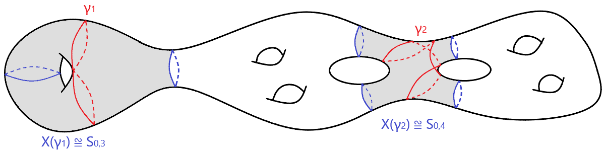
Figure 1. examples for $X(\gamma^{\prime})$

For a surface $X$ with possibly non-empty boundary, recall that a closed curve $\gamma\subset X$ is filling if the complement $X\setminus\gamma$ of $\gamma$ in $X$ is a disjoint union of disks and cylinders such that each cylinder is homotopic to a boundary component of $X$.

The following result is proved in [NWX20].

Proposition 7.

[NWX20, Proposition 47] Let $X\in\mathcal{M}_{g}$ and $\gamma^{\prime}\subset X$ be a non-simple closed geodesic. Then the connected subsurface $X(\gamma^{\prime})$ of $X$ constructed above satisfies that,

• $\gamma^{\prime}\subset X(\gamma^{\prime})$ is filling;

• the possibly empty boundary $\partial X(\gamma^{\prime})$ of $X(\gamma^{\prime})$ consists of simple closed multi-geodesics with

  $$\ell\left(\partial X(\gamma^{\prime})\right)\leq 2\ell_{\gamma^{\prime}}(X);$$

• the area $\mathop{\rm Area}(X(\gamma^{\prime}))\leq 4\ell_{\gamma^{\prime}}(X)$. In particular, if $\ell_{\gamma^{\prime}}(X)\prec\ln(g)$, then for large enough $g>1$, $X(\gamma^{\prime})$ is a proper subsurface of $X$.

Proof.

We only outline a proof here for completeness. One may see [NWX20] for more details.

For $(1)$: by construction the subsurface $X(\gamma^{\prime})$ is freely homotopic to $\mathcal{N}_{\epsilon}(\gamma^{\prime})$ in $X$. So it is also freely homotopic to $\gamma^{\prime}$ in $X$. Since $\gamma^{\prime}$ is the unique closed geodesic representing the free homotopy class $\gamma^{\prime}$ and $X(\gamma^{\prime})\subset X$ is a subsurface of geodesic boundary, we have

$$\gamma^{\prime}\subset X(\gamma^{\prime}).$$

By construction we know that $\gamma^{\prime}$ is filling in $X(\gamma^{\prime})$.

For (2): by construction clearly we have

$$\ell(\partial X(\gamma^{\prime}))\leq 2\ell_{\gamma^{\prime}}(X).$$

For (3): by construction we know that the complement $X(\gamma^{\prime})\setminus\gamma^{\prime}=(\sqcup D_{i})\sqcup(\sqcup C_{j})$ where the subsets are setwisely disjoint, the $D_{i}^{\prime}s$ are disjoint discs and the $C_{j}^{\prime}s$ are disjoint cylinders. By elementary Isoperimetric Inequality (e.g. see [Bus92, WX21]) we know that

$$\mathop{\rm Area}(D_{i})\leq\ell(\partial D_{i})\quad\text{and}\quad\mathop{\rm Area}(C_{j})\leq\ell(\partial C_{j}).$$

Thus, we have

$$\mathop{\rm Area}(X(\gamma^{\prime})) = \sum(\mathop{\rm Area}(D_{i}))+\sum(\mathop{\rm Area}(C_{j}))$$

$$\leq \sum(\ell(\partial D_{i}))+\sum(\ell(\partial C_{j}))$$

$$\leq 4\ell_{\gamma^{\prime}}(X).$$

If $\ell_{\gamma^{\prime}}(X)\prec\ln(g)$, we have $\mathop{\rm Area}(X(\gamma^{\prime}))\prec\ln(g)$. Then the conclusion clearly follows because $\mathop{\rm Area}(X)=4\pi(g-1)$ by Gauss-Bonnet.

The proof is complete. ∎

Remark.

It is not hard to see that the inequality $\mathop{\rm Area}(X(\gamma^{\prime}))\leq 4\ell_{\gamma^{\prime}}(X)$ can be improved to be $\mathop{\rm Area}(X(\gamma^{\prime}))\leq 2\ell_{\gamma^{\prime}}(X)$. For our purpose the constant $4$ in this bound is enough in this paper.

Definition.

For any $L>0$, we define

1. $\#(X,L)$ is the number of closed geodesics of length $\leq L$ on $X$;

2. $\#_{f}(X,L)$ is the number of filling closed geodesics of length $\leq L$ on $X$;

3. $\#_{0}(X,L)$ is the number of closed geodesics of length $\leq L$ on $X$ which are not iterates of any closed geodesic of length $\leq 2\mathop{\rm arcsinh}1$.

The map $\gamma^{\prime}\mapsto X(\gamma^{\prime})$ in the construction above is infinite-to-one. Indeed for any connected subsurface $Y\subset X$ of geodesic boundary, $X(\gamma_{1})=X(\gamma_{2})=Y$ for any two filling curves $\gamma_{1},\gamma_{2}\subset Y$. However, the multiplicity of the map $\gamma^{\prime}\mapsto X(\gamma^{\prime})$ is always bounded if restricting the length of $\gamma^{\prime}$ to be bounded. That is, $\#_{f}(Y,L)<\infty$ for any $L>0$. In this paper we prove the following counting result for compact hyperbolic surfaces of geodesic boundaries, which is essential in the proofs of Theorem 1 and 2 when dealing with primitive non-simple closed geodesics. Here a closed geodesic is called primitive if it is not an iterate of any other closed geodesic at least twice. Since the proof is technical, we postpone the proof until a single section 8.

Theorem 8 (=Theorem 4).

For any $\epsilon_{1}>0$ and $m=2g-2+n\geq 1$, there exists a constant $c(\epsilon_{1},m)$ only depending on $m$ and $\epsilon_{1}$ such that for any hyperbolic surface $X\in\mathcal{T}_{g,n}(x_{1},...,x_{n})$ we have

$$\#_{f}(X,T)\leq c(\epsilon_{1},m)\cdot e^{T-\frac{1-\epsilon_{1}}{2}\sum_{i=1}^{n}x_{i}}.$$

Remark.

Lalley in [Lal89] showed for a compact hyperbolic surface $X$ of geodesic boundary, the number $\#(X,L)\sim\frac{1}{2}\frac{e^{\delta L}}{\delta L}$ as $L\to\infty$ where $\delta$ is the Hausdorff dimension of the limit set of the Fuchsian group of $X$ in the boundary of the upper half plane (the factor $\frac{1}{2}$ disappears if counting oriented closed geodesics). The upper bound in Theorem 8 contains explicit information on the boundary length of $X$ and is uniform in $X$, which will play an essential role in the proofs of Theorem 1 and 2.

Now we conclude this section by several general and soft counting results. First we recall the following bound (e.g. see [Bus92, Lemma 6.6.4]).

Lemma 9.

For any $X\in\mathcal{M}_{g}$ and $L>0$, we have

$$\#_{0}(X,L)\leq(g-1)e^{L+6}.$$

The following result is a direct consequence of Lemma 9.

Lemma 10.

Let $X$ be a compact hyperbolic surface of non-empty geodesic boundary. Then

$$\#_{f}(X,L)\leq\frac{\mathop{\rm Area}(X)}{4\pi}e^{L+6}.$$

Proof.

We first double two $X$’s to get a closed hyperbolic surface $2X$. Since $\mathop{\rm Area}(2X)=2\mathop{\rm Area}(X)$, by Gauss-Bonnet the genus of $2X$ is equal to $\frac{\mathop{\rm Area}(X)}{2\pi}+1$. By symmetry, each closed geodesic counted in $\#_{f}(X,L)$ gives two curves counted in $\#_{0}(2X,L)$. By the Collar Lemma (e.g. see [Bus92, Theorem 4.1.6]) it is known that a closed geodesic in $2X$ of length $\leq 2\mathop{\rm arcsinh}1$ is always simple. So each filling curve in $X$ is clearly not an iterate of any closed geodesic in $2X$ of length $\leq 2\mathop{\rm arcsinh}1$. Then it follows by Lemma 9 that

$$2\#_{f}(X,L) \leq \#_{0}(2X,L)$$

$$\leq \frac{\mathop{\rm Area}(X)}{2\pi}e^{L+6}$$

which completes the proof. ∎

Recall that

$$\mathcal{M}_{g}^{\geq 1}\overset{\text{def}}{=}\{X\in\mathcal{M}_{g};\ell_{sys}(X)\geq 1\}$$

where $\ell_{sys}(X)$ is the length of shortest closed geodesic in $X$. Another direct consequence of Lemma 9 is as follows which will be applied later to bound Term-II.

Lemma 11.

For any $X\in\mathcal{M}_{g}^{\geq 1}$ and $L>0$, we have

$$\#(X,L)\leq 2(g-1)e^{L+6}.$$

Proof.

Let $\#_{1}(X,L)$ be the number of closed geodesics of length $\leq L$ on $X$ which are iterates of closed geodesics of length $\leq 2\mathop{\rm arcsinh}1$. First by the Collar Lemma (e.g. see [Bus92, Theorem 4.1.6]) we know that there are at most $(3g-3)$ simple closed geodesics of length $\leq 2\mathop{\rm arcsinh}1\sim 1.7627$. Moreover, they are mutually disjoint, and we denote them by $\Gamma$. Recall $X\in\mathcal{M}_{g}^{\geq 1}$, so $\ell_{sys}(X)\geq 1$. Then each closed geodesic counted in $\#_{1}(X,L)$ is an iterate of some curve in $\Gamma$ at most $L$ times. Thus we have

$$\#_{1}(X,L)\leq(3g-3)(L+1)$$

which together with Lemma 9 imply that

$$\#(X,L) = \#_{0}(X,L)+\#_{1}(X,L)$$

$$\leq (g-1)e^{L+6}+(3g-3)(L+1)$$

$$\leq 2(g-1)e^{L+6}$$

completing the proof. ∎

4. Weil-Petersson volume

In this section we list some results on Weil-Petersson volumes of moduli spaces which will be applied later in the proofs of Theorem 1 and 2. All of them are already known results and presented in [NWX20]. We denote $V_{g,n}(x_{1},\cdots,x_{n})$ to be the Weil-Petersson volume of $\mathcal{M}_{g,n}(x_{1},\cdots,x_{n})$ and $V_{g,n}=V_{g,n}(0,\cdots,0)$.

First we recall several results of Mirzakhani and her coauthors.

Theorem 12.

[Mir07a, Theorem 1.1] The volume $V_{g,n}(x_{1},\cdots,x_{n})$ is a polynomial in $x_{1}^{2},\cdots,x_{n}^{2}$ with degree $3g-3+n$. Namely we have

$$V_{g,n}(x_{1},\cdots,x_{n})=\sum_{\alpha;|\alpha|\leq 3g-3+n}C_{\alpha}\cdot x^{2\alpha}$$

where $C_{\alpha}>0$ lies in $\pi^{6g-6+2n-|2\alpha|}\cdot\mathbb{Q}$. Here $\alpha=(\alpha_{1},\cdots,\alpha_{n})$ is a multi-index and $|\alpha|=\alpha_{1}+\cdots+\alpha_{n}$, $x^{2\alpha}=x_{1}^{2\alpha_{1}}\cdots x_{n}^{2\alpha_{n}}$.

Lemma 13.

1. [Mir13, Lemma 3.2]

   $$V_{g,n}\leq V_{g,n}(x_{1},\cdots,x_{n})\leq e^{\frac{x_{1}+\cdots+x_{n}}{2}}V_{g,n}.$$

2. [Mir13, Theorem 3.5] For fixed $n\geq 0$, as $g\rightarrow\infty$ we have

   $$\frac{V_{g,n}}{V_{g-1,n+2}}=1+O(\frac{1}{g}).$$

   Where the implied constants are related to $n$ and independent of $g$.

Remark.

For Part $(2)$, one may also see the following Theorem 15 of Mirzakhani-Zograf.

Lemma 14.

[Mir13, Corollary 3.7] For fixed $b,k,r\geq 0$ and $C<C_{0}=2\ln 2$,

$$\sum_{\begin{array}[]{c}g_{1}+g_{2}=g+1-k\\ r+1\leq g_{1}\leq g_{2}\end{array}}e^{Cg_{1}}\cdot g_{1}^{b}\cdot V_{g_{1},k}\cdot V_{g_{2},k}\asymp\frac{V_{g}}{g^{2r+k}}$$

as $g\rightarrow\infty$. The implied constants are related to $b,k,r,C$ and independent of $g$.

The following several useful bounds for Weil-Petersson volumes are proved in [NWX20]. And their proofs highly rely on works in [Mir13] and the following asymptotic property of $V_{g,n}$ which dues to Mirzakhani-Zograf.

Theorem 15.

[MZ15, Theorem 1.2] There exists a universal constant $\alpha>0$ such that for any given $n\geq 0$,

$$V_{g,n}=\alpha\frac{1}{\sqrt{g}}(2g-3+n)!(4\pi^{2})^{2g-3+n}\big{(}1+O(\frac{1}{g})\big{)}$$

as $g\rightarrow\infty$. The implied constant is related to $n$ and independent of $g$.

The first one is as following which is motivated by [MP19, Proposition 3.1] where the error term in the lower bound is different.

Lemma 16.

[NWX20, Lemma 20] Let $g,n\geq 1$ and $x_{1},\cdots,x_{n}\geq 0$, then there exists a constant $c=c(n)>0$ independent of $g,x_{1},\cdots,x_{n}$ such that

$$\prod_{i=1}^{n}\frac{\sinh(x_{i}/2)}{x_{i}/2}\big{(}1-c(n)\frac{\sum_{i=1}^{n}x_{i}^{2}}{g}\big{)}\leq\frac{V_{g,n}(x_{1},\cdots,x_{n})}{V_{g,n}}\leq\prod_{i=1}^{n}\frac{\sinh(x_{i}/2)}{x_{i}/2}.$$

Remark.

In the lemma above,

1. for the lower bound, the $x_{i}^{\prime}s$ may be related to $g$ but $n$ is independent of $g$ as $g\rightarrow\infty$;

2. for the upper bound, both the $x_{i}^{\prime}s$ and $n$ may be related to $g$ as $g\rightarrow\infty$.

As in [NWX20], for $r\geq 1$ one may define

$$W_{r}\overset{\text{def}}{=}\begin{cases}V_{\frac{r}{2}+1}&\text{if $r$ is even},\\[5.0pt] V_{\frac{r+1}{2},1}&\text{if $r$ is odd}.\end{cases}$$

The proof of the following result relies on Lemma 13 and Lemma 14.

Lemma 17.

[NWX20, Lemma 21]

1. For any $g,n\geq 0$, we have

   $$V_{g,n}\leq c\cdot W_{2g-2+n}$$

   for some universal constant $c>0$.

2. For any $r\geq 1$ and $m_{0}\leq\frac{1}{2}r$, we have

   $$\sum_{m=m_{0}}^{[\frac{r}{2}]}W_{m}W_{r-m}\leq c(m_{0})\frac{1}{r^{m_{0}}}W_{r}$$

   for some constant $c(m_{0})>0$ only depending on $m_{0}$.

The proof of the following lemma relies on Theorem 15. Which is also a generalization of [MP19, Lemma 3.2] and [GLMST21, Lemma 6.3]. Here we allow the $n_{i}^{\prime}s$ and $q$ depend on $g$ as $g\to\infty$.

Lemma 18.

[NWX20, Lemma 22] Assume $q\geq 1$, $n_{1},\cdots,n_{q}\geq 0$, $r\geq 2$. Then there exists two universal constants $c,D>0$ such that

$$\sum_{\{g_{i}\}}V_{g_{1},n_{1}}\cdots V_{g_{q},n_{q}}\leq c\big{(}\frac{D}{r}\big{)}^{q-1}W_{r}$$

where the sum is taken over all $\{g_{i}\}_{i=1}^{q}\subset\mathbb{N}$ such that $2g_{i}-2+n_{i}\geq 1$ for all $i=1,\cdots,q$, and $\sum_{i=1}^{q}(2g_{i}-2+n_{i})=r$.

We conclude this section by the following useful property whose proof relies on Lemma 13 and Lemma 18.

Proposition 19.

[NWX20, Lemma 23] Given $m\geq 1$, for any $g\geq m+1$, $q\geq 1$, $n_{1},...,n_{q}\geq 1$, there exists a constant $c(m)>0$ only depending on $m$ such that

$$\sum_{\{g_{i}\}}V_{g_{1},n_{1}}\cdots V_{g_{q},n_{q}}\leq c(m)\frac{1}{g^{m}}V_{g}$$

where the sum is taken over all $\{g_{i}\}_{i=1}^{q}\subset\mathbb{N}$ such that $2g_{i}-2+n_{i}\geq 1$ for all $i=1,\cdots,q$, and $\sum_{i=1}^{q}(2g_{i}-2+n_{i})=2g-2-m$.

5. Selberg’s trace formula

In this section we describe the Selberg trace formula for closed hyperbolic surfaces, which is a main tool in the proofs of Theorem 1 and 2.

Let $C_{c}^{\infty}(\mathbb{R})$ denote the set of all smooth functions on $\mathbb{R}$ with compact support. Given a function $\phi\in C_{c}^{\infty}(\mathbb{R})$, its Fourier transform is defined as

$$\widehat{\phi}(z)\overset{\text{def}}{=}\int_{-\infty}^{\infty}\phi(x)e^{-ixz}dx$$

for any $z\in\mathbb{C}$. For $\phi\in C_{c}^{\infty}(\mathbb{R})$, the above integral is an entire function over $\mathbb{C}$. In particular, it converges for any $z\in\mathbb{C}$.

Recall that a closed geodesic is primitive if it is not an iterate of any other closed geodesic at least twice. For any hyperbolic surface $X$, we let $\mathcal{P}(X)$ denote the set of all oriented primitive closed geodesics on $X$. Now we recall Selberg’s trace formula in the form of [Ber16, Theorem 5.6] or [Bus92, Theorem 9.5.3]. One may also see e.g. [Sel56, Hej76] for more details.

Theorem 20 (Selberg’s trace formula).

Let $X$ be a closed hyperbolic surface of genus $g$ and let

$$0=\lambda_{0}(X)<\lambda_{1}(X)\leq\lambda_{2}(X)\leq\cdots\to\infty$$

denote the spectrum of the Laplacian on $X$. For $k\in\mathbb{Z}^{\geq 0}$, let

$$r_{k}(X)\overset{\text{def}}{=}\begin{cases}\sqrt{\lambda_{k}(X)-\frac{1}{4}},&\text{if $\lambda_{k}(X)>\frac{1}{4}$};\\ \textbf{i}\cdot\sqrt{-\lambda_{k}(X)+\frac{1}{4}},&\text{if $\lambda_{k}(X)\leq\frac{1}{4}$}.\end{cases}$$

Then for any even function $\phi\in C_{c}^{\infty}(\mathbb{R})$ we have

$$\sum_{k=0}^{\infty}\widehat{\phi}(r_{k}(X))= (g-1)\int_{-\infty}^{\infty}r\widehat{\phi}(r)\tanh(\pi r)dr$$

$$+\sum_{\gamma\in\mathcal{P}(X)}\sum_{k=1}^{\infty}\frac{\ell_{\gamma}(X)}{2\sinh\left(\frac{k\ell_{\gamma}(X)}{2}\right)}\phi(k\ell_{\gamma}(X)).$$

Both sides of the formula above are absolutely convergent.

Choice of $\phi$. In this paper, we apply the same function in [MNP20] to Selberg’s trace formula. For completeness, we briefly introduce such a function. One may see [MNP20, Section 2] for more details.

First one may let $\psi:\mathbb{R}\to\mathbb{R}^{\geq 0}$ be a smooth and even function whose support is exactly $(-\frac{1}{2},\frac{1}{2})$. Then we define

$$\phi_{0}(x)\overset{\text{def}}{=}\int_{\mathbb{R}}\psi(x-t)\psi(t)dt.$$

It is not hard to see that

Lemma 21.

The function $\phi_{0}$ satisfies that

1. $\phi_{0}$ is non-negative and even.

2. $\mathop{\rm Supp}(\phi_{0})=(-1,1)$.

3. The Fourier transform $\widehat{\phi_{0}}$ satisfies $\widehat{\phi_{0}}(\xi)\geq 0$ for all $\xi\in\mathbb{R}\cup\textbf{i}\mathbb{R}$.

Now for any $T>0$ we define

$$\phi_{T}(x)\overset{\text{def}}{=}\phi_{0}\left(\frac{x}{T}\right).$$

The following property [MNP20, Lemma 2.4] will be applied later.

Lemma 22.

For any small enough $\epsilon>0$, then there exists a constant $C_{\epsilon}>0$ depending on $\epsilon$ and $\phi_{0}$ such that for $t\geq 0$,

$$\widehat{\phi_{4\ln(g)}}(\textbf{i}t)\geq C_{\epsilon}g^{4(1-\epsilon)t}\ln(g).$$

In particular, for any hyperbolic surface $X\in\mathcal{M}_{g}$ with $\lambda_{1}(X)\leq\frac{3}{16}-\epsilon$ we have

$$\widehat{\phi_{4\ln(g)}}(r_{1}(X))\geq C_{\epsilon}g^{1+C_{\epsilon}}\ln(g)$$

where $r_{1}(X)=\rm{\textbf{i}}\cdot\sqrt{-\lambda_{1}(X)+\frac{1}{4}}$ in Selberg’s trace formula.

Proof.

We outline a proof here for completeness. Since $\phi_{0}\geq 0$ and $\mathop{\rm Supp}(\phi_{0})=(-1,1)$, we have that for any $\epsilon>0$ near $0$,

$$\widehat{\phi_{4\ln(g)}}(\textbf{i}t) = 4\ln(g)\int_{\mathbb{R}}\phi_{0}(x)e^{\left(4\ln(g)t\cdot x\right)}dx$$

$$\geq 4\ln(g)\int_{1-\epsilon}^{1}\phi_{0}(x)e^{\left(4\ln(g)t\cdot x\right)}dx$$

$$\geq B_{\epsilon}g^{4(1-\epsilon)t}\ln(g)$$

where $B_{\epsilon}=4\int_{1-\epsilon}^{1}\phi_{0}(x)dx>0$ depends on $\epsilon$ and $\phi_{0}$. For any hyperbolic surface $X\in\mathcal{M}_{g}$ with $\lambda_{1}(X)\leq\frac{3}{16}-\epsilon$, then $r_{1}(X)=\rm{\textbf{i}}\cdot\sqrt{-\lambda_{1}(X)+\frac{1}{4}}$ where $\sqrt{-\lambda_{1}(X)+\frac{1}{4}}\geq\sqrt{\frac{1}{16}+\epsilon}$. Then the conclusion follows by choosing

$$C_{\epsilon}=\min\{B_{\epsilon},\left(\sqrt{1+16\epsilon}(1-\epsilon)-1\right)\}.$$

The proof is complete. ∎

6. Proofs of Theorem 1 and 2–relatively easy parts

In the following two sections we finish the proofs of Theorem 1 and 2. In this section we study the relative easy parts.

Let $X\in\mathcal{M}_{g}$ be a hyperbolic surface of genus $g$. A closed geodesic $\gamma\subset X$ is called non-simple if $\gamma$ intersects itself; otherwise it is called simple. A simple closed geodesic $\alpha\subset X$ is called non-separating if the complement $X\setminus\alpha$ is connected; otherwise it is called separating. Recall that $\mathcal{P}(X)$ is the set of all oriented primitive closed geodesics on $X$. Now we split it as the following cases:

1. $\mathcal{P}^{s}_{sep}(X)\overset{\text{def}}{=}\{\gamma\in\mathcal{P}(X)\ \text{is simple and separating}\}.$

2. $\mathcal{P}^{s}_{nsep}(X)\overset{\text{def}}{=}\{\gamma\in\mathcal{P}(X)\ \text{is simple and non-separating}\}.$

3. $\mathcal{P}^{ns}(X)\overset{\text{def}}{=}\{\gamma\in\mathcal{P}(X)\ \text{is non-simple}\}.$

Clearly we have

$$\mathcal{P}(X)=\mathcal{P}^{s}_{sep}(X)\cup\mathcal{P}^{s}_{nsep}(X)\cup\mathcal{P}^{ns}(X).$$

Let $\phi_{T}(x)$ be the function in Section 5. We plug $\phi_{T}$ into Selberg’s trace formula Theorem 20 and rewrite it as

(8) $$\quad\quad\sum_{k=0}^{\infty}\widehat{\phi_{T}}(r_{k}(X))=(g-1)\int_{-\infty}^{\infty}r\widehat{\phi_{T}}(r)\tanh(\pi r)dr+$$

$$\sum_{\gamma\in\mathcal{P}(X)}\frac{\ell_{\gamma}(X)}{2\sinh\left(\frac{\ell_{\gamma}(X)}{2}\right)}\phi_{T}(\ell_{\gamma}(X))+\sum_{\gamma\in\mathcal{P}(X)}\sum_{k=2}^{\infty}\frac{\ell_{\gamma}(X)}{2\sinh\left(\frac{k\ell_{\gamma}(X)}{2}\right)}\phi_{T}(k\ell_{\gamma}(X))$$

$$=\underbrace{(g-1)\int_{-\infty}^{\infty}r\widehat{\phi_{T}}(r)\tanh(\pi r)dr}_{\rm I}+\underbrace{\sum_{\gamma\in\mathcal{P}(X)}\sum_{k=2}^{\infty}\frac{\ell_{\gamma}(X)}{2\sinh\left(\frac{k\ell_{\gamma}(X)}{2}\right)}\phi_{T}(k\ell_{\gamma}(X))}_{\rm{II}}$$

$$+\underbrace{\sum_{\gamma\in\mathcal{P}^{s}_{sep}(X)}\frac{\ell_{\gamma}(X)}{2\sinh\left(\frac{\ell_{\gamma}(X)}{2}\right)}\phi_{T}(\ell_{\gamma}(X))}_{\rm{III}}+\underbrace{\sum_{\gamma\in\mathcal{P}^{s}_{nsep}(X)}\frac{\ell_{\gamma}(X)}{2\sinh\left(\frac{\ell_{\gamma}(X)}{2}\right)}\phi_{T}(\ell_{\gamma}(X))}_{\rm{IV}}$$

$$+\underbrace{\sum_{\gamma\in\mathcal{P}^{ns}(X)}\frac{\ell_{\gamma}(X)}{2\sinh\left(\frac{\ell_{\gamma}(X)}{2}\right)}\phi_{T}(\ell_{\gamma}(X))}_{\rm{V}}.$$

Next we will take an integral of Equation (8) over the moduli space $\mathcal{M}_{g}$ endowed with the Weil-Petersson metric. Recall that $\widehat{\phi_{T}}(r_{k}(X))\geq 0$ for all $k\geq 0$. For the $\operatorname{LHS}$ of (8), we will only keep the first two terms $\widehat{\phi_{T}}(r_{0}(X))$ and $\widehat{\phi_{T}}(r_{1}(X))$. For the $\operatorname{RHS}$ of (8), we will bound the five terms case by case: Term-I can be bounded by using an elementary observation; we will combine an argument in [MNP20] and a result in [Mir13] to bound Term-II; for Term-III and Term-IV we will apply Mirzakhani’s integration formula [Mir07a] to bound them; the last Term-V is the most difficult case on which we will apply the new counting result Theorem 8 and combine similar ideas in [Mir07a, NWX20] to get the desired bound. We postpone the study of Term-V until the next section.

6.1. An upper bound for $\int_{\mathcal{M}_{g}}\rm{I}dX$

In this subsection we provide the following bound on Term I in the $\rm RHS$ of (8).

Proposition 23.

Let $\phi_{T}$ be the function in Section 5. Then we have for all $T>1$ and as $g\to\infty$,

$$\left|\frac{1}{V_{g}}\int_{\mathcal{M}_{g}}\left((g-1)\int_{-\infty}^{\infty}r\widehat{\phi_{T}}(r)\tanh(\pi r)dr\right)dX\right|\prec\frac{g}{T}.$$

Proof.

Since $\phi_{0}$ is compactly supported, its Fourier transform $\widehat{\phi_{0}}$ is a Schwartz function which decays faster than any polynomial. In particular there exists a constant $C>0$ such that

$$\int_{0}^{\infty}|x||\widehat{\phi_{0}}(x)|dx\leq C<\infty.$$

Recall that $\phi_{T}$ is an even function and $\left|\tanh(\pi r)\right|\leq 1$. Since $\widehat{\phi_{T}}(r)=T\widehat{\phi_{0}}(Tr)$,

$$\left|\int_{-\infty}^{\infty}r\widehat{\phi_{T}}(r)\tanh(\pi r)dr\right| = T\left|\int_{-\infty}^{\infty}r\widehat{\phi_{0}}(Tr)\tanh(\pi r)dr\right|$$

$$\leq \frac{2}{T}\int_{0}^{\infty}|x||\widehat{\phi_{0}}(x)|dx$$

$$\leq \frac{2C}{T}$$

which clearly implies the conclusion. ∎

6.2. An upper bound for $\int_{\mathcal{M}_{g}}\rm{II}dX$

In this subsection we prove the following bound on Term II in the $\rm RHS$ of (8).

Proposition 24.

Let $\phi_{T}$ be the function in Section 5. Then we have for all $T>1$ and as $g\to\infty$,

$$\frac{1}{V_{g}}\int_{\mathcal{M}_{g}}\sum_{\gamma\in\mathcal{P}(X)}\sum_{k=2}^{\infty}\frac{\ell_{\gamma}(X)}{2\sinh\left(\frac{k\ell_{\gamma}(X)}{2}\right)}\phi_{T}(k\ell_{\gamma}(X))dX\prec T^{2}g.$$

We split the proof into several lemmas.

Lemma 25.

For any $X\in\mathcal{M}_{g}^{\geq 1}$ and $T>1$, then we have

$$\sum_{\gamma\in\mathcal{P}(X)}\sum_{k=2}^{\infty}\frac{\ell_{\gamma}(X)}{2\sinh\left(\frac{k\ell_{\gamma}(X)}{2}\right)}\phi_{T}(k\ell_{\gamma}(X))\prec T^{2}g.$$

Proof.

Since $X\in\mathcal{M}_{g}^{\geq 1}$, we have that for all $\gamma\in\mathcal{P}(X)$,

$$\sinh\left(\frac{k\ell_{\gamma}(X)}{2}\right)\asymp e^{\frac{k\ell_{\gamma}(X)}{2}}.$$

Now we follow [MNP20]. Recall that $\phi_{T}$ is bounded and $\mathop{\rm Supp}(\phi_{T})=(-T,T)$. So we have

(9) $$\sum_{\gamma\in\mathcal{P}(X)}\sum_{k=2}^{\infty}\frac{\ell_{\gamma}(X)}{2\sinh\left(\frac{k\ell_{\gamma}(X)}{2}\right)}\phi_{T}(k\ell_{\gamma}(X))$$

$$\asymp\sum_{\gamma\in\mathcal{P}(X)}\sum_{k=2}^{\infty}\ell_{\gamma}(X)e^{-\frac{k\ell_{\gamma}(X)}{2}}\phi_{T}(k\ell_{\gamma}(X))$$

$$\prec\sum_{\gamma\in\mathcal{P}(X),\ \ell_{\gamma}(X)\leq\frac{T}{2}}\ell_{\gamma}(X)e^{-\ell_{\gamma}(X)}$$

$$\leq\sum_{m=1}^{[T]}me^{-m}\cdot\#\{\gamma\in\mathcal{P}(X);m\leq\ell_{\gamma}(X)<m+1\}.$$

It follows by Lemma 11 that

(10) $$\#\{\gamma\in\mathcal{P}(X);m\leq\ell_{\gamma}(X)<m+1\}\prec ge^{m}$$

which together with (9) imply that

$$\sum_{\gamma\in\mathcal{P}(X)}\sum_{k=2}^{\infty}\frac{\ell_{\gamma}(X)}{2\sinh\left(\frac{k\ell_{\gamma}(X)}{2}\right)}\phi_{T}(k\ell_{\gamma}(X)) \prec \sum_{m=1}^{[T]}me^{-m}\cdot g\cdot e^{m}$$

$$\asymp T^{2}g.$$

The proof is complete. ∎

Lemma 26.

For any $X\in\mathcal{M}_{g}^{<1}$ and $T>1$, then we have

$$\sum_{\gamma\in\mathcal{P}(X)}\sum_{k=2}^{\infty}\frac{\ell_{\gamma}(X)}{2\sinh\left(\frac{k\ell_{\gamma}(X)}{2}\right)}\phi_{T}(k\ell_{\gamma}(X))\prec\left(T^{2}g+\sum_{\begin{subarray}{c}\alpha\in\mathcal{P}(X);\\ \ell_{\alpha}(X)<1\end{subarray}}\frac{T}{\ell_{\alpha}(X)}\right).$$

Proof.

First we rewrite

(11) $$\sum_{\gamma\in\mathcal{P}(X)}\sum_{k=2}^{\infty}\frac{\ell_{\gamma}(X)}{2\sinh\left(\frac{k\ell_{\gamma}(X)}{2}\right)}\phi_{T}(k\ell_{\gamma}(X))$$

$$=\sum_{\begin{subarray}{c}\alpha\in\mathcal{P}(X);\\ \ell_{\alpha}(X)<1\end{subarray}}\sum_{k=2}^{\infty}\frac{\ell_{\gamma}(X)}{2\sinh\left(\frac{k\ell_{\gamma}(X)}{2}\right)}\phi_{T}(k\ell_{\gamma}(X))$$

$$+\sum_{\begin{subarray}{c}\alpha\in\mathcal{P}(X);\\ \ell_{\alpha}(X)\geq 1\end{subarray}}\sum_{k=2}^{\infty}\frac{\ell_{\gamma}(X)}{2\sinh\left(\frac{k\ell_{\gamma}(X)}{2}\right)}\phi_{T}(k\ell_{\gamma}(X)).$$

For the second term of the $\operatorname{RHS}$ above, one may apply the same argument in the proof of Lemma 25 to get

(12) $$\sum_{\begin{subarray}{c}\alpha\in\mathcal{P}(X);\\ \ell_{\alpha}(X)\geq 1\end{subarray}}\sum_{k=2}^{\infty}\frac{\ell_{\gamma}(X)}{2\sinh\left(\frac{k\ell_{\gamma}(X)}{2}\right)}\phi_{T}(k\ell_{\gamma}(X))\prec T^{2}g.$$

For the first term of the $\operatorname{RHS}$ of (11) above, recall that $\phi_{T}$ is bounded and $\mathop{\rm Supp}(\phi_{T})=(-T,T)$. Since $\sinh(kx)\geq kx$ for all $x\geq 0$ and $k\geq 0$, we have

$$\sum_{\begin{subarray}{c}\alpha\in\mathcal{P}(X);\\ \ell_{\alpha}(X)<1\end{subarray}}\sum_{k=2}^{\infty}\frac{\ell_{\gamma}(X)}{2\sinh\left(\frac{k\ell_{\gamma}(X)}{2}\right)}\phi_{T}(k\ell_{\gamma}(X))\prec\sum_{\begin{subarray}{c}\alpha\in\mathcal{P}(X);\\ \ell_{\alpha}(X)<1\end{subarray}}\sum_{k=2}^{[\frac{T}{\ell_{\gamma}(X)}]+1}\frac{1}{k}$$

For all $n\geq 2$, it is not hard to see that

$$\frac{1}{2}+\frac{1}{3}+\cdots+\frac{1}{n}<4\ln(n).$$

Thus, we have

(13) $$\sum_{\begin{subarray}{c}\alpha\in\mathcal{P}(X);\\ \ell_{\alpha}(X)<1\end{subarray}}\sum_{k=2}^{\infty}\frac{\ell_{\gamma}(X)}{2\sinh\left(\frac{k\ell_{\gamma}(X)}{2}\right)}\phi_{T}(k\ell_{\gamma}(X))$$

$$\prec\sum_{\begin{subarray}{c}\alpha\in\mathcal{P}(X);\\ \ell_{\alpha}(X)<1\end{subarray}}\ln\left([\frac{T}{\ell_{\gamma}(X)}]+1\right)$$

$$\leq\sum_{\begin{subarray}{c}\alpha\in\mathcal{P}(X);\\ \ell_{\alpha}(X)<1\end{subarray}}\ln\left(\frac{2T}{\ell_{\gamma}(X)}\right)$$

$$\leq 2\sum_{\begin{subarray}{c}\alpha\in\mathcal{P}(X);\\ \ell_{\alpha}(X)<1\end{subarray}}\frac{T}{\ell_{\alpha}(X)}$$

where in the last inequality we apply the fact that $e^{x}\geq x$ for all $x\geq 0$.

Then the conclusion clearly follows by (11), (12) and (13). ∎

The Collar Lemma [Bus92] implies that $\alpha$ is always simple if $\ell_{\alpha}(X)<1$. As in [Mir13, Page 292] we define $f:\mathcal{M}_{g}\to\mathbb{R}^{\geq 0}$ as

$$f(X)\overset{\text{def}}{=}\sum_{\ell_{\alpha}(X)\leq 1}\frac{1}{\ell_{\alpha}(X)}.$$

By using her Integration Formula (see Theorem 6), Mirzakhani [Mir13, Page 292] showed that

Lemma 27.

$$\int_{\mathcal{M}_{g}}f(X)dX\asymp V_{g}.$$

Now we are ready to prove Proposition 24.

Proof of Proposition 24.

It follows by Lemma 25, 26 and 27 that

$$\frac{1}{V_{g}}\int_{\mathcal{M}_{g}}\sum_{\gamma\in\mathcal{P}(X)}\sum_{k=2}^{\infty}\frac{\ell_{\gamma}(X)}{2\sinh\left(\frac{k\ell_{\gamma}(X)}{2}\right)}\phi_{T}(k\ell_{\gamma}(X))dX$$

$$=\frac{1}{V_{g}}\int_{\mathcal{M}_{g}^{\geq 1}}\sum_{\gamma\in\mathcal{P}(X)}\sum_{k=2}^{\infty}\frac{\ell_{\gamma}(X)}{2\sinh\left(\frac{k\ell_{\gamma}(X)}{2}\right)}\phi_{T}(k\ell_{\gamma}(X))dX$$

$$+\frac{1}{V_{g}}\int_{\mathcal{M}_{g}^{<1}}\sum_{\gamma\in\mathcal{P}(X)}\sum_{k=2}^{\infty}\frac{\ell_{\gamma}(X)}{2\sinh\left(\frac{k\ell_{\gamma}(X)}{2}\right)}\phi_{T}(k\ell_{\gamma}(X))dX$$

$$\prec T^{2}g\cdot\frac{\mathop{\rm Vol}(\mathcal{M}_{g}^{\geq 1})}{V_{g}}+\left(T^{2}g\cdot\frac{\mathop{\rm Vol}(\mathcal{M}_{g}^{<1})}{V_{g}}+\frac{T}{V_{g}}\int_{\mathcal{M}_{g}^{<1}}f(X)dX\right)$$

$$\prec T^{2}g.$$

The proof is complete. ∎

6.3. An upper bound for $\int_{\mathcal{M}_{g}}\rm{III}dX$

In this subsection we apply the Integration Formula of Mirzakhani (see Theorem 6) as a tool to prove the following bound on Term III in the $\rm RHS$ of (8).

Proposition 28.

Let $\phi_{T}$ be the function in Section 5. Then we have for all $T>1$ and as $g\to\infty$,

$$\frac{1}{V_{g}}\int_{\mathcal{M}_{g}}\sum_{\gamma\in\mathcal{P}^{s}_{sep}(X)}\frac{\ell_{\gamma}(X)}{2\sinh\left(\frac{\ell_{\gamma}(X)}{2}\right)}\phi_{T}(\ell_{\gamma}(X))dX\prec\frac{e^{\frac{T}{2}}}{g}.$$

Proof.

For each $1\leq k\leq[\frac{g}{2}]$, we let $\alpha_{k}\subset X$ be an unoriented simple closed geodesic separating $X$ into $X_{k,1}\cup X_{g-k,1}$ where $X_{k,1}$ is a subsurface in $X$ of $k$ genus with one boundary curve $\alpha_{k}$. Recall that $\mathcal{P}^{s}_{sep}(X)$ is the set of oriented simple and separating closed geodesics. So for $\gamma\in\mathcal{P}^{s}_{sep}(X)$, $\gamma\neq\gamma^{-1}\in\mathcal{P}^{s}_{sep}(X)$. But they have the same lengths. By symmetry we have

$$\sum_{\gamma\in\mathcal{P}^{s}_{sep}(X)}\frac{\ell_{\gamma}(X)}{2\sinh\left(\frac{\ell_{\gamma}(X)}{2}\right)}\phi_{T}(\ell_{\gamma}(X))=2\sum_{k=1}^{[\frac{g}{2}]}\sum_{\gamma\in\mathop{\rm Mod}_{g}\cdot\alpha_{k}}\frac{\ell_{\gamma}(X)}{2\sinh\left(\frac{\ell_{\gamma}(X)}{2}\right)}\phi_{T}(\ell_{\gamma}(X)).$$

Now one may apply the Integration Formula of Mirzakhani (see Theorem 6) to get

(14) $$\frac{1}{V_{g}}\int_{\mathcal{M}_{g}}\sum_{\gamma\in\mathcal{P}^{s}_{sep}(X)}\frac{\ell_{\gamma}(X)}{2\sinh\left(\frac{\ell_{\gamma}(X)}{2}\right)}\phi_{T}(\ell_{\gamma}(X))dX$$

$$\leq\frac{2}{V_{g}}\sum_{k=1}^{[\frac{g}{2}]}\int_{0}^{\infty}\frac{x}{2\sinh\left(\frac{x}{2}\right)}\phi_{T}(x)V_{k,1}(x)V_{g-k,1}(x)xdx.$$

Recall that Lemma 16 tells that for all $1\leq k\leq[\frac{g}{2}]$,

$$V_{k,1}(x)\leq\frac{\sinh(x/2)}{x/2}V_{k,1}\ \text{and}\ V_{g-k,1}(x)\leq\frac{\sinh(x/2)}{x/2}V_{g-k,1}.$$

Thus, combine (14) and the two inequalities above we get

(15) $$\frac{1}{V_{g}}\int_{\mathcal{M}_{g}}\sum_{\gamma\in\mathcal{P}^{s}_{sep}(X)}\frac{\ell_{\gamma}(X)}{2\sinh\left(\frac{\ell_{\gamma}(X)}{2}\right)}\phi_{T}(\ell_{\gamma}(X))dX$$

$$\leq 2\int_{0}^{\infty}2\sinh\left(\frac{x}{2}\right)\phi_{T}(x)dx\cdot\left(\frac{\sum_{k=1}^{[\frac{g}{2}]}V_{k,1}V_{g-k,1}}{V_{g}}\right)$$

$$\leq 2\int_{0}^{\infty}e^{\frac{x}{2}}\phi_{T}(x)dx\cdot\left(\frac{\sum_{k=1}^{[\frac{g}{2}]}V_{k,1}V_{g-k,1}}{V_{g}}\right).$$

By Lemma 14 we know that

(16) $$\frac{\sum_{k=1}^{[\frac{g}{2}]}V_{k,1}V_{g-k,1}}{V_{g}}\asymp\frac{1}{g}.$$

Plug (16) into (15), since $\phi_{T}$ is bounded and $\mathop{\rm Supp}(\phi_{T})=(-T,T)$ we get

$$\frac{1}{V_{g}}\int_{\mathcal{M}_{g}}\sum_{\gamma\in\mathcal{P}^{s}_{sep}(X)}\frac{\ell_{\gamma}(X)}{2\sinh\left(\frac{\ell_{\gamma}(X)}{2}\right)}\phi_{T}(\ell_{\gamma}(X))dX \prec \frac{1}{g}\cdot\int_{0}^{T}e^{\frac{x}{2}}dx$$

$$\asymp \frac{e^{\frac{T}{2}}}{g}.$$

The proof is complete. ∎

6.4. A bound for $\int_{\mathcal{M}_{g}}\rm{IV}dX$

In this subsection we also apply the Integration Formula of Mirzakhani (see Theorem 6) as a tool to prove the following bound to link Term IV in the $\rm RHS$ of (8) and $\widehat{\phi_{T}}(\frac{\textbf{i}}{2})$.

Proposition 29.

Let $\phi_{T}$ be the function in Section 5. Then we have for all $T>1$ and as $g\to\infty$,

$$\left|\frac{1}{V_{g}}\int_{\mathcal{M}_{g}}\sum_{\gamma\in\mathcal{P}^{s}_{nsep}(X)}\frac{\ell_{\gamma}(X)}{2\sinh\left(\frac{\ell_{\gamma}(X)}{2}\right)}\phi_{T}(\ell_{\gamma}(X))dX-\widehat{\phi_{T}}(\frac{\textbf{i}}{2})\right|\prec\left(\frac{T^{2}e^{\frac{T}{2}}}{g}+1\right).$$

We first list the following elementary properties for $\phi_{T}$:

1. $\int_{0}^{\infty}e^{-\frac{x}{2}}\phi_{T}(x)dx\prec 1$.

2. $\int_{0}^{\infty}e^{\frac{x}{2}}\phi_{T}(x)dx\prec e^{\frac{T}{2}}.$

3. $\widehat{\phi_{T}}(\frac{\textbf{i}}{2})=\int_{-\infty}^{\infty}e^{\frac{x}{2}}\phi_{T}(x)dx=\int_{0}^{\infty}2\cosh\left(\frac{x}{2}\right)\phi_{T}(x)dx\prec e^{\frac{T}{2}}.$

Now we prove Proposition 29.

Proof of Proposition 29.

Let $\alpha_{0}\subset X$ be an unoriented simple non-separating closed geodesic. Similar as in the proof of Proposition 28, for $\gamma\in\mathcal{P}^{s}_{nsep}(X)$, $\gamma\neq\gamma^{-1}\in\mathcal{P}^{s}_{nsep}(X)$. But they have the same lengths. So by symmetry we have

$$\sum_{\gamma\in\mathcal{P}^{s}_{nsep}(X)}\frac{\ell_{\gamma}(X)}{2\sinh\left(\frac{\ell_{\gamma}(X)}{2}\right)}\phi_{T}(\ell_{\gamma}(X))=2\left(\sum_{\gamma\in\mathop{\rm Mod}_{g}\cdot\alpha_{0}}\frac{\ell_{\gamma}(X)}{2\sinh\left(\frac{\ell_{\gamma}(X)}{2}\right)}\phi_{T}(\ell_{\gamma}(X))\right).$$

Since $\alpha_{0}$ is simple and non-separating and $g>2$, one may apply the Integration Formula of Mirzakhani (see Theorem 6) to get

(17) $$\int_{\mathcal{M}_{g}}\sum_{\gamma\in\mathop{\rm Mod}_{g}\cdot\alpha_{0}}\frac{\ell_{\gamma}(X)}{2\sinh\left(\frac{\ell_{\gamma}(X)}{2}\right)}\phi_{T}(\ell_{\gamma}(X))dX$$

$$=\frac{1}{2}\int_{0}^{\infty}\frac{x}{2\sinh\left(\frac{x}{2}\right)}\phi_{T}(x)V_{g-1,2}(x,x)xdx.$$

Thus, we have

(18) $$\int_{\mathcal{M}_{g}}\sum_{\gamma\in\mathcal{P}^{s}_{nsep}(X)}\frac{\ell_{\gamma}(X)}{2\sinh\left(\frac{\ell_{\gamma}(X)}{2}\right)}\phi_{T}(\ell_{\gamma}(X))dX$$

$$=\int_{0}^{\infty}\frac{x}{2\sinh\left(\frac{x}{2}\right)}\phi_{T}(x)V_{g-1,2}(x,x)xdx.$$

By Lemma 16 we know that

$$\frac{V_{g-1,2}(x,x)}{V_{g-1,2}}=\left(\frac{\sinh(x/2)}{x/2}\right)^{2}\cdot\left(1+O\left(\frac{x^{2}}{g}\right)\right)$$

where the implied constant is uniform. By Lemma 13 we have

$$V_{g-1,2}=V_{g}\cdot\left(1+O\left(\frac{1}{g}\right)\right)$$

where the implied constant is also uniform. So we have

(19) $$\frac{V_{g-1,2}(x,x)}{V_{g}}=\left(\frac{\sinh(x/2)}{x/2}\right)^{2}\cdot\left(1+O\left(\frac{1+x^{2}}{g}\right)\right).$$

Plug (19) into (18) we get

(20) $$\frac{1}{V_{g}}\int_{\mathcal{M}_{g}}\sum_{\gamma\in\mathcal{P}^{s}_{nsep}(X)}\frac{\ell_{\gamma}(X)}{2\sinh\left(\frac{\ell_{\gamma}(X)}{2}\right)}\phi_{T}(\ell_{\gamma}(X))dX$$

$$=\int_{0}^{\infty}2\sinh\left(\frac{x}{2}\right)\phi_{T}(x)\cdot\left(1+O\left(\frac{1+x^{2}}{g}\right)\right)dx.$$

$$=\int_{0}^{\infty}e^{\frac{x}{2}}\phi_{T}(x)\cdot\left(1+O\left(\frac{1+x^{2}}{g}\right)\right)dx$$

$$-\int_{0}^{\infty}e^{\frac{-x}{2}}\phi_{T}(x)\cdot\left(1+O\left(\frac{1+x^{2}}{g}\right)\right)dx.$$

Recall that we have $\widehat{\phi_{T}}(\frac{\textbf{i}}{2})=\int_{0}^{\infty}2\cosh\left(\frac{x}{2}\right)\phi_{T}(x)dx$, $\int_{0}^{\infty}\phi_{T}(x)e^{\frac{x}{2}}dx\prec e^{\frac{T}{2}}$ and $\int_{0}^{\infty}e^{-\frac{x}{2}}\phi_{T}(x)dx\prec 1$. Now it follows by (20) that

$$\left|\frac{1}{V_{g}}\int_{\mathcal{M}_{g}}\sum_{\gamma\in\mathcal{P}^{s}_{nsep}(X)}\frac{\ell_{\gamma}(X)}{2\sinh\left(\frac{\ell_{\gamma}(X)}{2}\right)}\phi_{T}(\ell_{\gamma}(X))dX-\widehat{\phi_{T}}(\frac{\textbf{i}}{2})\right|$$

$$\prec\int_{0}^{\infty}e^{\frac{x}{2}}\phi_{T}(x)\cdot\left(\frac{1+x^{2}}{g}\right)dx$$

$$+\int_{0}^{\infty}e^{\frac{-x}{2}}\phi_{T}(x)\cdot\left(2+\frac{1+x^{2}}{g}\right)dx$$

$$\prec\frac{T^{2}e^{\frac{T}{2}}}{g}+\left(2+\frac{T^{2}}{g}\right)$$

$$\prec\frac{T^{2}e^{\frac{T}{2}}}{g}+1.$$

The proof is complete. ∎

7. Proofs of Theorem 1, 2 and 3

In this section we resolve intersections of non-simple closed geodesics, and apply the new counting result Theorem 8 and similar ideas in [Mir07a, NWX20] to study the most difficult case: Term V in the $\rm RHS$ of (8). Then we will combine the new desired bound on Term V and the results in the previous section to complete the proofs of Theorem 1 and 2.

7.1. An upper bound for Term V

In this subsection we apply the new counting result Theorem 8 to give an effective upper bound for Term V of (8).

Throughout this section we always assume that $g>1$ is large enough and

(21) $$T=a\ln(g)$$

where $a>0$ is any fixed constant.

Let $X\in\mathcal{M}_{g}$ be a hyperbolic surface and $\gamma\in\mathcal{P}^{ns}(X)$ be a non-simple closed geodesic of length $\ell_{\gamma}(X)\leq T$. By Proposition 7 one may assume that $X(\gamma)\subset X$ is a connected subsurface of geodesic boundary (we warn here that two distinct simple closed geodesics on the boundary of $X(\gamma)$ may correspond to a single simple closed geodesic in $X$) such that

1. $\gamma\subset X(\gamma)$ is filing;

2. $\ell(\partial X(\gamma))\leq 2\ell_{\gamma}(X)\leq 2T$;

3. $\mathop{\rm Area}(X(\gamma))\leq 4\ell_{\gamma}(X)\leq 4T$.

Definition.

For $T=a\ln(g)>0$ and $X\in\mathcal{M}_{g}$, we define

$$\rm{Sub_{T}(X)}\overset{\text{def}}{=}\left\{\parbox[1]{241.84842pt}{$Y\subset X$ is a connected subsurface of geodesic boundary such that $\ell(\partial Y)\leq 2T$ and $\mathop{\rm Area}(Y)\leq 4T$ }\right\}$$

where we allow two distinct simple closed geodesics on the boundary of $Y$ to be a single simple closed geodesic in $X$.

For large enough $g>1$, we have that the map

$$Y\mapsto\partial Y$$

is injective; indeed if $\partial Y_{1}=\partial Y_{2}$ for $Y_{1}\neq Y_{2}\in\rm{Sub_{T}(X)}$, then $Y_{1}$ and $Y_{2}$ lie on the two different sides of $\partial Y_{1}=\partial Y_{2}$ and we have $Y_{1}\cup Y_{2}=X$ implying that

$$4\pi(g-1)=\mathop{\rm Area}(X)\leq\mathop{\rm Area}(Y_{1})+\mathop{\rm Area}(Y_{2})\leq 8a\ln(g)$$

which is impossible for large enough $g>1$.

Let $\gamma\in\mathcal{P}^{ns}(X)$ be of length $\ell_{\gamma}(X)\leq T$ and consider the composition $\mathcal{F}$ of the following two maps

$$\gamma\mapsto X(\gamma)\mapsto\partial X(\gamma),$$

then we have that for any $\gamma\in\mathcal{P}^{ns}(X)$ of length $\ell_{\gamma}(X)\leq T$,

(22) $$\#\left\{\gamma^{\prime}\in\mathcal{P}^{ns}(X);\ \ell_{\gamma^{\prime}}(X)\leq T\ \textit{and}\ \mathcal{F}(\gamma^{\prime})=\mathcal{F}(\gamma)\right\}\leq 2\#_{f}\left(X(\gamma),T\right)$$

where $\#_{f}\left(X(\gamma),T\right)$ is the number of filling (unoriented) closed geodesics in $X(\gamma)$ of length less than or equal to $T$.

We prove the following upper bound for Term V in the $\rm RHS$ of (8).

Proposition 30.

Let $\phi_{T}$ be the function in Section 5. For any $\epsilon_{1}>0$, there exists a constant $c(\epsilon_{1})>0$ only depending on $\epsilon_{1}$ such that as $g\to\infty$,

(23) $$\sum_{\gamma\in\mathcal{P}^{ns}(X)}\frac{\ell_{\gamma}(X)}{2\sinh\left(\frac{\ell_{\gamma}(X)}{2}\right)}\phi_{T}(\ell_{\gamma}(X))$$

$$\prec T^{2}e^{T}\left(\sum_{\begin{subarray}{c}Y\in\rm{Sub_{T}(X)};\\ |\chi(Y)|\geq 17\end{subarray}}e^{-\frac{\ell(\partial Y)}{4}}\textbf{1}_{[0,2T]}(\ell(\partial Y))\right)$$

$$+c(\epsilon_{1})T\left(\sum_{\begin{subarray}{c}Y\in\rm{Sub_{T}(X)};\\ 1\leq|\chi(Y)|\leq 16\end{subarray}}e^{\frac{T}{2}-\frac{1-\epsilon_{1}}{2}\ell(\partial Y)}\mathrm{\textbf{1}_{[0,2T]}}(\ell(\partial Y))\right).$$

Proof.

Recall that every non-simple closed geodesic has length at least $4\mathop{\rm arcsinh}(1)$ (e.g. see [Bus92, 4.2.2]). Since $\phi_{T}\geq 0$ is bounded and $\mathop{\rm Supp}(\phi_{T})=(-T,T)$, we get

(24) $$\sum_{\gamma\in\mathcal{P}^{ns}(X)}\frac{\ell_{\gamma}(X)}{2\sinh\left(\frac{\ell_{\gamma}(X)}{2}\right)}\phi_{T}(\ell_{\gamma}(X))\asymp\sum_{\gamma\in\mathcal{P}^{ns}(X)}\ell_{\gamma}(X)e^{-\frac{\ell_{\gamma}(X)}{2}}\phi_{T}(\ell_{\gamma}(X))$$

$$\prec\sum_{\gamma\in\mathcal{P}^{ns}(X)}\ell_{\gamma}(X)e^{-\frac{\ell_{\gamma}(X)}{2}}\textbf{1}_{[0,T]}(\ell_{\gamma}(X))$$

$$=2\times\left(\sum_{Y\in\rm{Sub_{T}(X)}}\sum_{\gamma\subset Y\ \textit{is filling}}\ell_{\gamma}(X)e^{-\frac{\ell_{\gamma}(X)}{2}}\textbf{1}_{[0,T]}(\ell_{\gamma}(X))\right)$$

$$=2\times\sum_{\begin{subarray}{c}Y\in\rm{Sub_{T}(X)};\\ |\chi(Y)|\geq 17\end{subarray}}\ \sum_{\gamma\subset Y\ \textit{is filling}}\ell_{\gamma}(X)e^{-\frac{\ell_{\gamma}(X)}{2}}\textbf{1}_{[0,T]}(\ell_{\gamma}(X))$$

$$+2\times\sum_{\begin{subarray}{c}Y\in\rm{Sub_{T}(X)};\\ 1\leq|\chi(Y)|\leq 16\end{subarray}}\ \sum_{\gamma\subset Y\ \textit{is filling}}\ell_{\gamma}(X)e^{-\frac{\ell_{\gamma}(X)}{2}}\textbf{1}_{[0,T]}(\ell_{\gamma}(X)).$$

Where the factor $2$ is from the multiplicity because the curves in $\mathcal{P}^{ns}(X)$ are oriented. Now we consider the first term in the RHS of (24). Since $\gamma\subset Y$ is filling,

(25) $$\frac{\ell(\partial Y)}{2}\leq\ell_{\gamma}(Y)=\ell_{\gamma}(X).$$

For $Y\in\rm{Sub_{T}(X)}$ we know that $\mathop{\rm Area}(Y)\leq 4T$. So by Lemma 10 we have

(26) $$\#_{f}\left(Y,T\right)\prec Te^{T}.$$

By (25) and (26) we have

(27) $$\sum_{\begin{subarray}{c}Y\in\rm{Sub_{T}(X)};\\ |\chi(Y)|\geq 17\end{subarray}}\ \sum_{\gamma\subset Y\ \textit{is filling}}\ell_{\gamma}(X)e^{-\frac{\ell_{\gamma}(X)}{2}}\textbf{1}_{[0,T]}(\ell_{\gamma}(X))$$

$$\leq\sum_{\begin{subarray}{c}Y\in\rm{Sub_{T}(X)};\\ |\chi(Y)|\geq 17\end{subarray}}\#_{f}\left(Y,T\right)Te^{-\frac{\ell(\partial Y)}{4}}\textbf{1}_{[0,2T]}(\ell(\partial Y))$$

$$\prec T^{2}e^{T}\left(\sum_{\begin{subarray}{c}Y\in\rm{Sub_{T}(X)};\\ |\chi(Y)|\geq 17\end{subarray}}e^{-\frac{\ell(\partial Y)}{4}}\textbf{1}_{[0,2T]}(\ell(\partial Y))\right).$$

Now we consider the second term in the RHS of (24). Let $Y\in\rm{Sub_{T}(X)}$ with $m=|\chi(Y)|\in[1,16]$. For any $\epsilon_{1}>0$, let $c(\epsilon_{1})=\max\limits_{1\leq m\leq 16}c(m,\epsilon_{1})>0$ where $c(m,\epsilon_{1})>0$ is the constant in Theorem 8. Then we have that for large enough $g>1$,

(28) $$\sum_{\gamma\subset Y\ \textit{is filling}}\ell_{\gamma}(X)e^{-\frac{\ell_{\gamma}(X)}{2}}\textbf{1}_{[0,T]}(\ell_{\gamma}(X))$$

$$\leq\sum_{n=0}^{[T]}(n+1)e^{-\frac{n}{2}}\cdot\#\{\gamma\subset Y\ \textit{is filling};\ n<\ell_{\gamma}(Y)\leq n+1\}\cdot\textbf{1}_{[0,2T]}(\ell(\partial Y)).$$

By the new counting result Theorem 8 we know that for each $n\geq 0$,

(29) $$\#\{\gamma\subset Y\ \textit{is filling};\ n<\ell_{\gamma}(Y)\leq n+1\}\leq c(\epsilon_{1})e^{n+1-\frac{1-\epsilon_{1}}{2}\ell(\partial Y)}.$$

By (28) and (29) we have

$$\sum_{\gamma\subset Y\ \textit{is filling}}\ell_{\gamma}(X)e^{-\frac{\ell_{\gamma}(X)}{2}}\textbf{1}_{[0,T]}(\ell_{\gamma}(X))$$

$$\leq c(\epsilon_{1})e^{1-\frac{1-\epsilon_{1}}{2}\ell(\partial Y)}\sum_{n=0}^{[T]}(n+1)e^{\frac{n}{2}}\textbf{1}_{[0,2T]}(\ell(\partial Y))$$

$$\prec c(\epsilon_{1})Te^{\frac{T}{2}-\frac{1-\epsilon_{1}}{2}\ell(\partial Y)}\textbf{1}_{[0,2T]}(\ell(\partial Y))$$

which implies that

(30) $$\sum_{\begin{subarray}{c}Y\in\rm{Sub_{T}(X)};\\ 1\leq|\chi(Y)|\leq 16\end{subarray}}\ \sum_{\gamma\subset Y\ \textit{is filling}}\ell_{\gamma}(X)e^{-\frac{\ell_{\gamma}(X)}{2}}\textbf{1}_{[0,T]}(\ell_{\gamma}(X))$$

$$\prec c(\epsilon_{1})T\left(\sum_{\begin{subarray}{c}Y\in\rm{Sub_{T}(X)};\\ 1\leq|\chi(Y)|\leq 16\end{subarray}}e^{\frac{T}{2}-\frac{1-\epsilon_{1}}{2}\ell(\partial Y)}\textbf{1}_{[0,2T]}(\ell(\partial Y))\right).$$

Then the conclusion follows by (24), (27) and (30). ∎

Remark.

The critical value $16$ for Euler characteristic in the Proposition above is not the unique choice. Actually the remaining argument also works if replacing $16$ by any positive integer larger than $16$.

7.2. An upper bound for $\int_{\mathcal{M}_{g}}\rm{V}dx$

In this subsection we prove our desired upper bound for $\int_{\mathcal{M}_{g}}\rm{V}dx$. Recall that the map $Y\mapsto\partial Y$ is injective for $Y\in\rm{Sub_{T}(X)}$ and large enough $g>1$. We take an integral of (23) in Proposition 30 over $\mathcal{M}_{g}$, and then apply the Integration Formula of Mirzakhani (see Theorem 6) to get the desired upper bounds.

First we restrict the argument to a single orbit $\mathop{\rm Mod}_{g}\cdot Y\subset\rm{Sub_{T}(X)}$.

Assumption $(\star)$.

let $Y_{0}\in\rm{Sub_{T}(X)}$ satisfying

• $Y_{0}$ is homeomorphic to $S_{g_{0},k}$ for some $g_{0}\geq 0$ and $k>0$ with $m=|\chi(Y_{0})|=2g_{0}-2+k\geq 1$;

• the boundary $\partial Y_{0}$ is a simple closed multi-geodesics in $X$ consisting of $k$ simple closed geodesics which has $n_{0}$ pairs of simple closed geodesics for some $n_{0}\geq 0$ such that each pair corresponds to a single simple closed geodesic in $X$;

• the interior of its complement $X\setminus S_{g_{0},k}$ consists of $q$ components $S_{g_{1},n_{1}},\cdots,$ $S_{g_{q},n_{q}}$ for some $q\geq 1$ where $\sum_{i=1}^{q}n_{i}=k-2n_{0}$.

(e.g. see Figure 2).

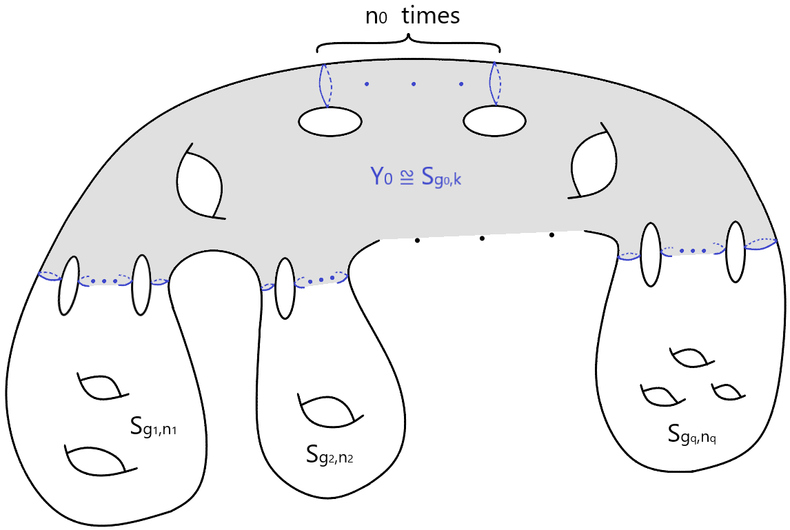
Figure 2. an example for $Y_{0}$

Let $h:\mathbb{R}^{\geq 0}\to\mathbb{R}^{\geq 0}$ be a continuous function. Next we compute the integral $\int_{\mathcal{M}_{g}}\sum_{Y\in\mathop{\rm Mod}_{g}\cdot Y_{0}}h(\ell(\partial Y))\textbf{1}_{[0,2T]}(\ell(\partial Y))dX$.

Recall that the map $Y\mapsto\partial Y$ is injective for $Y\in\rm{Sub_{T}(X)}$ and large enough $g>1$, and $\ell(\partial Y)\leq 2T$. It follows by the Integration Formula of Mirzakhani (see Theorem 6) that

$$\int_{\mathcal{M}_{g}}\sum_{Y\in\mathop{\rm Mod}_{g}\cdot Y_{0}}h(\ell(\partial Y))\textbf{1}_{[0,2T]}(\ell(\partial Y))dX$$

$$=\int_{\mathcal{M}_{g}}\sum_{\partial Y\in\mathop{\rm Mod}_{g}\cdot\partial Y_{0}}h(\ell(\partial Y))\textbf{1}_{[0,2T]}(\ell(\partial Y))dX$$

$$\leq\frac{1}{|\mathop{\rm Sym}|}\int_{\mathbb{R}_{\geq 0}^{k-n_{0}}}h\left(\sum_{j=1}^{n_{0}}2x_{j}^{\prime}+\sum_{i=1}^{q}(x_{i,1}+\cdots+x_{i,n_{i}})\right)$$

$$\mathbf{1}_{[0,2T]}\left(\sum_{j=1}^{n_{0}}2x_{j}^{\prime}+\sum_{i=1}^{q}(x_{i,1}+\cdots+x_{i,n_{i}})\right)$$

$$V_{g_{0},k}(x_{1}^{\prime},x_{1}^{\prime},\cdots,x_{n_{0}}^{\prime},x_{n_{0}}^{\prime},x_{1,1},\cdots,x_{1,n_{1}},x_{2,1},\cdots,x_{q,n_{q}})$$

$$V_{g_{1},n_{1}}(x_{1,1},\cdots,x_{1,n_{1}})\cdots V_{g_{q},n_{q}}(x_{q,1},\cdots,x_{q,n_{q}})$$

$$x_{1}^{\prime}\cdots x_{n_{0}}^{\prime}\cdot x_{1,1}\cdots x_{q,n_{q}}dx_{1}^{\prime}\cdots dx_{n_{0}}^{\prime}dx_{1,1}\cdots dx_{q,n_{q}}.$$

Recall that the symmetry is given by $\mathop{\rm Sym}(\partial Y_{0})=\mathop{\rm Stab}(\partial Y_{0})/\cap_{\gamma\in\partial Y_{0}}\mathop{\rm Stab}(\gamma)$. For each $1\leq i\leq q$, the set of all permutations of $n_{i}$ boundary geodesics of $S_{g_{i},n_{i}}$ gives $n_{i}!$ elements in $\mathop{\rm Sym}(\partial Y_{0})$. Meanwhile, the set of all permutations of $n_{0}$ pairs of geodesics defined in Assumption ($\star$) gives $n_{0}!$ elements. So we have

$$|\mathop{\rm Sym}|\geq n_{0}!n_{1}!\cdots n_{q}!.$$

By Lemma 13, we have

$$V_{g,n}(x_{1},\cdots,x_{n})\leq e^{\frac{x_{1}+\cdots+x_{n}}{2}}V_{g,n},$$

Set the condition

$$Cond:=\{0\leq x_{j}^{\prime},\ 0\leq x_{i,j},\ \sum_{j=1}^{n_{0}}2x_{j}^{\prime}+\sum_{i=1}^{q}\sum_{j=1}^{n_{i}}x_{i,j}\leq 2T\}.$$

Put all these equations together we get

(31) $$\quad\int_{\mathcal{M}_{g}}\sum_{Y\in\mathop{\rm Mod}_{g}\cdot Y_{0}}h(\ell(\partial Y))\textbf{1}_{[0,2T]}(\ell(\partial Y))dX$$

$$\leq\frac{1}{n_{0}!n_{1}!\cdots n_{q}!}V_{g_{0},k}V_{g_{1},n_{1}}\cdots V_{g_{q},n_{q}}\times$$

$$\int_{Cond}h\left(\sum_{j=1}^{n_{0}}2x_{j}^{\prime}+\sum_{i=1}^{q}(x_{i,1}+\cdots+x_{i,n_{i}})\right)\cdot e^{\sum_{j=1}^{n_{0}}x_{j}^{\prime}+\sum_{i=1}^{q}(x_{i,1}+\cdots+x_{i,n_{i}})}$$

$$x_{1}^{\prime}\cdots x_{n_{0}}^{\prime}\cdot x_{1,1}\cdots x_{q,n_{q}}dx_{1}^{\prime}\cdots dx_{n_{0}}^{\prime}dx_{1,1}\cdots dx_{q,n_{q}}.$$

Now we apply (31) to bound the integral of the first term in the RHS of (23) in Proposition 30.

Proposition 31.

Let $Y_{0}\in\rm{Sub_{T}(X)}$ satisfying Assumption ($\star$). Then we have that as $g\to\infty$,

$$\int_{\mathcal{M}_{g}}\sum_{Y\in\mathop{\rm Mod}_{g}\cdot Y_{0}}e^{-\frac{\ell(\partial Y)}{4}}\textbf{1}_{[0,2T]}(\ell(\partial Y))dX\prec e^{\frac{7}{2}T}V_{g_{0},k}\frac{V_{g_{1},n_{1}}\cdots V_{g_{q},n_{q}}}{n_{0}!n_{1}!\cdots n_{q}!}.$$

Proof.

We apply (31) for the case that $h(x)=e^{-\frac{x}{4}}$ to get

(32) $$\int_{\mathcal{M}_{g}}\sum_{Y\in\mathop{\rm Mod}_{g}\cdot Y_{0}}e^{-\frac{\ell(\partial Y)}{4}}\textbf{1}_{[0,2T]}(\ell(\partial Y))dX$$

$$\prec\frac{1}{n_{0}!n_{1}!\cdots n_{q}!}V_{g_{0},k}V_{g_{1},n_{1}}\cdots V_{g_{q},n_{q}}$$

$$\times\int_{Cond}e^{\frac{1}{2}\cdot(\sum_{j=1}^{n_{0}}x_{j}^{\prime})+\frac{3}{4}\cdot(\sum_{i=1}^{q}(x_{i,1}+\cdots+x_{i,n_{i}}))}$$

$$x_{1}^{\prime}\cdots x_{n_{0}}^{\prime}\cdot x_{1,1}\cdots x_{q,n_{q}}dx_{1}^{\prime}\cdots dx_{n_{0}}^{\prime}dx_{1,1}\cdots dx_{q,n_{q}}.$$

Recall that

$$\int_{x_{i}\geq 0,\ \sum_{j=1}^{n}x_{i}\leq s}x_{1}\cdots x_{n}dx_{1}\cdots dx_{n}=\frac{(s)^{2n}}{(2n)!}<e^{s}.$$

Since $Cond\subset\{x_{i}^{\prime}\geq 0,x_{i,j}\geq 0,\ \sum_{j=1}^{n_{0}}x_{j}^{\prime}+\sum_{i=1}^{q}\sum_{j=1}^{n_{i}}x_{i,j}\leq 2T\}$,

(33) $$\int_{Cond}x_{1}^{\prime}\cdots x_{n_{0}}^{\prime}\cdot x_{1,1}\cdots x_{q,n_{q}}dx_{1}^{\prime}\cdots dx_{n_{0}}^{\prime}dx_{1,1}\cdots dx_{q,n_{q}}<e^{2T}.$$

Since $\frac{1}{2}\cdot(\sum_{j=1}^{n_{0}}x_{j}^{\prime})+\frac{3}{4}\cdot(\sum_{i=1}^{q}(x_{i,1}+\cdots+x_{i,n_{i}}))\leq\frac{3}{4}\ell(\partial Y)\leq\frac{3}{2}T$ on $Cond$, we combine (32) and (33) to get

$$\int_{\mathcal{M}_{g}}\sum_{Y\in\mathop{\rm Mod}_{g}\cdot Y_{0}}e^{-\frac{\ell(\partial Y)}{4}}\textbf{1}_{[0,2T]}(\ell(\partial Y))dX$$

$$\prec\frac{1}{n_{0}!n_{1}!\cdots n_{q}!}V_{g_{0},k}V_{g_{1},n_{1}}\cdots V_{g_{q},n_{q}}\times(e^{\frac{3}{2}T}e^{2T})$$

$$=e^{\frac{7}{2}T}\frac{1}{n_{0}!n_{1}!\cdots n_{q}!}V_{g_{0},k}V_{g_{1},n_{1}}\cdots V_{g_{q},n_{q}}$$

as desired. ∎

Next we bound the integral of $e^{-\frac{\ell(\partial Y)}{4}}\textbf{1}_{[0,2T]}(\ell(\partial Y))$ over $\mathcal{M}_{g}$ when the topological type of $Y$ is fixed. Assume that $Y\cong S_{g_{0},k}$ meaning that $Y$ is homeomorphic to $S_{g_{0},k}$ (e.g. see Figure 3).

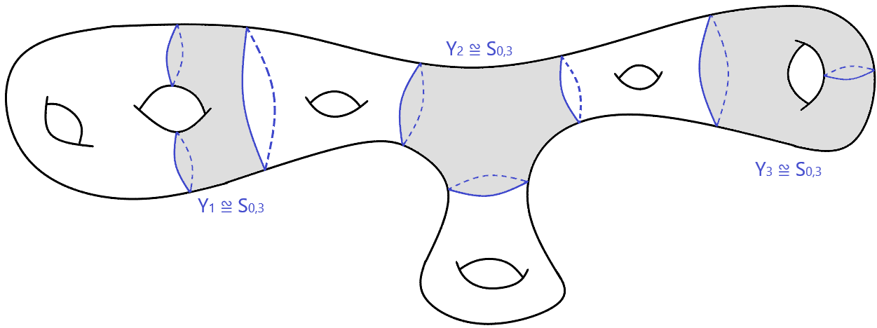
Figure 3. $Y_{1}\cong Y_{2}\cong Y_{3}\cong S_{0,3}$, but they are in different orbits

Then we let $g_{0}$ and $k$ be fixed in Assumption ($\star$), and let $q\geq 1$, $\{g_{i}\}_{1\leq i\leq q}$ and $\{n_{i}\}_{1\leq i\leq q}$ vary. We list several facts for $Y_{0}\in\rm{Sub_{T}(X)}$ satisfying Assumption ($\star$) which will be applied later.

• $Y_{0}$ is homeomorphic to $S_{g_{0},k}$ for some fixed $g_{0}\geq 0$ and $k>0$ with $m=|\chi(Y_{0})|=2g_{0}-2+k\geq 1$;

• by Gauss-Bonnet $2\pi m=2\pi(2g_{0}-2+k)\leq 4T$;

• $\sum_{i=1}^{q}n_{i}=k-2n_{0}$. In particular $n_{0}$ is determined by $\{n_{i}\}_{1\leq i\leq q}$;

• $\sum_{i=1}^{q}(2g_{i}-2+n_{i})=2g-2-m=2g-2g_{0}-k$. In particular, for large enough $g>1$, $2g-2g_{0}-k\geq 2g-2-\frac{4T}{2\pi}>g$ because $T=a\ln(g)$.

Recall that as in Section 4 for all $r\geq 1$,

$$W_{r}=\begin{cases}V_{\frac{r}{2}+1}&\text{if $r$ is even},\\[5.0pt] V_{\frac{r+1}{2},1}&\text{if $r$ is odd}.\end{cases}$$

Proposition 32.

Let $g_{0}\geq 0$ and $k\geq 1$ be fixed with $m=2g_{0}-2+k\geq 1$. Then we have that as $g\to\infty$,

$$\int_{\mathcal{M}_{g}}\sum\limits_{\begin{subarray}{c}Y\in\rm{Sub_{T}(X)};\\ Y\cong S_{g_{0},k}\end{subarray}}e^{-\frac{\ell(\partial Y)}{4}}\textbf{1}_{[0,2T]}(\ell(\partial Y))dX\prec e^{\frac{7}{2}T}W_{2g_{0}+k-2}W_{2g-2g_{0}-k}.$$

Proof.

It follows by Proposition 31 that

(34) $$\int_{\mathcal{M}_{g}}\sum\limits_{\begin{subarray}{c}Y\in\rm{Sub_{T}(X)};\\ Y\cong S_{g_{0},k}\end{subarray}}e^{-\frac{\ell(\partial Y)}{4}}\textbf{1}_{[0,2T]}(\ell(\partial Y))dX$$

$$\prec\sum_{q}\sum_{n_{1},\cdots,n_{q}}\sum_{g_{1},\cdots,g_{q}}e^{\frac{7}{2}T}\frac{1}{n_{0}!n_{1}!\cdots n_{q}!}V_{g_{0},k}V_{g_{1},n_{1}}\cdots V_{g_{q},n_{q}}$$

where the summation takes over all possible $q\geq 1$ and $(g_{1},n_{1}),\cdots,(g_{q},n_{q})$ such that $\sum_{i=1}^{q}(2g_{i}-2+n_{i})=2g-2-m=2g-2g_{0}-k$.

For fixed $q\geq 1$ and $\{n_{i}\}_{1\leq i\leq q}$, it follows by Lemma 18 that

$$\sum_{g_{1},\cdots,g_{q}}V_{g_{1},n_{1}}\cdots V_{g_{q},n_{q}} \leq c\left(\frac{D}{2g-2g_{0}-k}\right)^{q-1}W_{2g-2g_{0}-k}$$

$$< c\left(\frac{D}{g}\right)^{q-1}W_{2g-2g_{0}-k}$$

where we apply $2g-2g_{0}-k>g$ for large enough $g$ in the last inequality. Then by (34) and (7.2) we have

(36) $$\int_{\mathcal{M}_{g}}\sum\limits_{\begin{subarray}{c}Y\in\rm{Sub_{T}(X)};\\ Y\cong S_{g_{0},k}\end{subarray}}e^{-\frac{\ell(\partial Y)}{4}}\textbf{1}_{[0,2T]}(\ell(\partial Y))dX$$

$$\prec e^{\frac{7}{2}T}V_{g_{0},k}W_{2g-2g_{0}-k}\times\left(\sum_{q}\sum_{n_{1},\cdots,n_{q}}\frac{1}{n_{0}!n_{1}!\cdots n_{q}!}\left(\frac{D}{g}\right)^{q-1}\right).$$

Recall that for fixed $k-2n_{0}\geq 1$, we always have

$$\sum_{n_{1}+..+n_{q}=k-2n_{0},\ n_{i}\geq 0}\frac{(k-2n_{0})!}{n_{1}!\cdots n_{q}!}={\underbrace{(1+1+\cdots+1)}_{q\ \text{times}}}^{k-2n_{0}}=q^{k-2n_{0}}.$$

Since $0\leq n_{0}\leq[\frac{k-1}{2}]$ and $\frac{q^{k-2n_{0}}}{(k-2n_{0})!}<e^{q}$, we have that for large enough $g>1$,

$$\sum_{q}\sum_{n_{1},\cdots,n_{q}}\frac{1}{n_{0}!n_{1}!\cdots n_{q}!}\left(\frac{D}{g}\right)^{q-1}$$

$$= \sum_{q}\sum_{0\leq n_{0}\leq[\frac{k-1}{2}]}\frac{q^{k-2n_{0}}}{n_{0}!(k-2n_{0})!}\left(\frac{D}{g}\right)^{q-1}$$

$$< \left(\sum_{q}e^{q}\cdot\left(\frac{D}{g}\right)^{q-1}\right)\left(\sum_{0\leq n_{0}\leq[\frac{k-1}{2}]}\frac{1}{n_{0}!}\right)$$

$$< \sum_{q}e\cdot e\cdot\left(\frac{eD}{g}\right)^{q-1}$$

$$\prec 1.$$

Recall that Part $(1)$ of Lemma 17 states that $V_{g,n}\leq cW_{2g-2+n}$ for a universal constant $c>0$. Then we plug (7.2) into (36) to get the conclusion. ∎

For any $Y\in\rm{Sub_{T}(X)}$ it is known that $|\chi(Y)|\leq\frac{4T}{2\pi}$. Now we bound the integral of $\sum\limits_{Y\in\rm{Sub_{T}(X)}}e^{-\frac{\ell(\partial Y)}{4}}\textbf{1}_{[0,2T]}(\ell(\partial Y))$ over $\mathcal{M}_{g}$ when $m\leq|\chi(Y)|\leq[\frac{4T}{2\pi}]$ where $m\geq 1$ is a fixed integer. That is, we allow $g_{0}$ and $k$ in Assumption ($\star$) vary such that $m\leq 2g_{0}+k-2\leq[\frac{4T}{2\pi}]$.

Proposition 33.

Let $m\geq 1$ be any fixed integer. Then we have that there exists a constant $c(m)>0$ only depending on $m$ such that as $g\to\infty$,

$$\int_{\mathcal{M}_{g}}\sum\limits_{\begin{subarray}{c}Y\in\rm{Sub_{T}(X)};\\ m\leq|\chi(Y)|\leq[\frac{4T}{2\pi}]\end{subarray}}e^{-\frac{\ell(\partial Y)}{4}}\textbf{1}_{[0,2T]}(\ell(\partial Y))dX\prec Te^{\frac{7}{2}T}c(m)\frac{V_{g}}{g^{m}}.$$

Proof.

Let $Y\cong S_{g_{0},k}\in\rm{Sub_{T}(X)}$ with $|\chi(Y)|=2g_{0}+k-2\geq m$. In particular we have

$$1\leq k\leq[\frac{4T}{2\pi}]+2.$$

Then it follows by Proposition 32 that

(38) $$\int_{\mathcal{M}_{g}}\sum\limits_{\begin{subarray}{c}Y\in\rm{Sub_{T}(X)};\\ m\leq|\chi(Y)|\leq[\frac{4T}{2\pi}]\end{subarray}}e^{-\frac{\ell(\partial Y)}{4}}\textbf{1}_{[0,2T]}(\ell(\partial Y))dX$$

$$=\int_{\mathcal{M}_{g}}\sum\limits_{m\leq|\chi(Y)|\leq[\frac{4T}{2\pi}]}\sum\limits_{\begin{subarray}{c}Y\in\rm{Sub_{T}(X)};\\ Y\cong S_{g_{0},k}\end{subarray}}e^{-\frac{\ell(\partial Y)}{4}}\textbf{1}_{[0,2T]}(\ell(\partial Y))dX$$

$$\prec\sum\limits_{1\leq k\leq[\frac{4T}{2\pi}]+2}\ \sum\limits_{g_{0}:m\leq 2g_{0}-2+k\leq[\frac{4T}{2\pi}]}e^{\frac{7}{2}T}W_{2g_{0}+k-2}W_{2g-2g_{0}-k}.$$

By Part $(2)$ of Lemma 17 we know that for fixed $k\geq 1$,

(39) $$\sum\limits_{g_{0}:m\leq 2g_{0}-2+k\leq[\frac{4T}{2\pi}]}W_{2g_{0}+k-2}W_{2g-2g_{0}-k}\leq c(m)\frac{1}{(2g-2)^{m}}W_{2g-2}$$

for some constant $c(m)>0$ only depending on $m$. By definition we know that $W_{2g-2}=V_{g}$. Thus, it follows by (38) and (39) that

$$\int_{\mathcal{M}_{g}}\sum\limits_{\begin{subarray}{c}Y\in\rm{Sub_{T}(X)};\\ m\leq|\chi(Y)|\leq[\frac{4T}{2\pi}]\end{subarray}}e^{-\frac{\ell(\partial Y)}{4}}\textbf{1}_{[0,2T]}(\ell(\partial Y))dX$$

$$\prec e^{\frac{7}{2}T}\left(\sum\limits_{1\leq k\leq[\frac{4T}{2\pi}]+2}\frac{c(m)}{(2g-2)^{m}}V_{g}\right)$$

$$\prec Te^{\frac{7}{2}T}c(m)\frac{V_{g}}{g^{m}}.$$

The proof is complete. ∎

Our aim is to show that when $T=4\ln(g)$, the expected value of the RHS in Proposition 30 behaves like $o(g^{1+\epsilon})$ for any $\epsilon>0$ as $g\to\infty$. Proposition 33 implies that if $m\geq 17$, we truly have this property. More precisely, if $T=4\ln(g)$ we have

$$\small{\frac{T^{2}e^{T}}{V_{g}}\int_{\mathcal{M}_{g}}\sum\limits_{\begin{subarray}{c}Y\in\rm{Sub_{T}(X)};\\ m\leq|\chi(Y)|\leq[\frac{4T}{2\pi}]\end{subarray}}e^{-\frac{\ell(\partial Y)}{4}}\textbf{1}_{[0,2T]}(\ell(\partial Y))dX\prec(\ln(g))^{3}g}.$$

Next we will apply similar ideas in the proof of Proposition 32 to show the expected value of the second term of the RHS of (23) in Proposition 30 also has the same property even if $1\leq m\leq 16$.

In the sequel, we always assume that $Y_{0}\cong S_{g_{0},k}\in\rm{Sub_{T}(X)}$ satisfies Assumption ($\star$) with an additional assumption that

$$1\leq 2g_{0}+k-2\leq 16.$$

Then $1\leq k\leq 18$ and $0\leq g_{0}\leq 8$. Actually there are 88 pairs of such integers $(g_{0},k)$ satisfying the above inequality, even we will only apply the finiteness. Now we prove

Proposition 34.

Let $g_{0}\geq 0$ and $k\geq 1$ be fixed with $m=2g_{0}-2+k\in[1,16]$. For any $\epsilon_{1}>0$, then we have that as $g\to\infty$,

$$\int_{\mathcal{M}_{g}}\sum\limits_{\begin{subarray}{c}Y\in\rm{Sub_{T}(X)};\\ Y\cong S_{g_{0},k}\end{subarray}}e^{\frac{T}{2}-\frac{1-\epsilon_{1}}{2}\ell(\partial Y)}\textbf{1}_{[0,2T]}(\ell(\partial Y))dX\prec T^{66}e^{\frac{T}{2}+\epsilon_{1}T}\frac{V_{g}}{g^{m}}.$$

Proof.

Let $Y_{0}\cong S_{g_{0},k}\in\rm{Sub_{T}(X)}$ satisfying Assumption ($\star$). Recall that the map $Y\mapsto\partial Y$ is injective for $Y\in\rm{Sub_{T}(X)}$ and large enough $g>1$. Now we apply the Integration Formula of Mirzakhani (see Theorem 6) to get

(40) $$\int_{\mathcal{M}_{g}}\sum_{Y\in\mathop{\rm Mod}_{g}\cdot Y_{0}}e^{\frac{T}{2}-\frac{1-\epsilon_{1}}{2}\ell(\partial Y)}\textbf{1}_{[0,2T]}(\ell(\partial Y))dX$$

$$=\int_{\mathcal{M}_{g}}\sum_{\partial Y\in\mathop{\rm Mod}_{g}\cdot\partial Y_{0}}e^{\frac{T}{2}-\frac{1-\epsilon_{1}}{2}\ell(\partial Y)}\textbf{1}_{[0,2T]}(\ell(\partial Y))dX$$

$$\leq\frac{1}{|\mathop{\rm Sym}|}\int_{\mathbb{R}_{\geq 0}^{k-n_{0}}}e^{\frac{T}{2}-\frac{1-\epsilon_{1}}{2}\left(\sum_{j=1}^{n_{0}}2x_{j}^{\prime}+\sum_{i=1}^{q}(x_{i,1}+\cdots+x_{i,n_{i}})\right)}$$

$$\mathbf{1}_{[0,2T]}\left(\sum_{j=1}^{n_{0}}2x_{j}^{\prime}+\sum_{i=1}^{q}(x_{i,1}+\cdots+x_{i,n_{i}})\right)$$

$$V_{g_{0},k}(x_{1}^{\prime},x_{1}^{\prime},\cdots,x_{n_{0}}^{\prime},x_{n_{0}}^{\prime},x_{1,1},\cdots,x_{1,n_{1}},x_{2,1},\cdots,x_{q,n_{q}})$$

$$V_{g_{1},n_{1}}(x_{1,1},\cdots,x_{1,n_{1}})\cdots V_{g_{q},n_{q}}(x_{q,1},\cdots,x_{q,n_{q}})$$

$$x_{1}^{\prime}\cdots x_{n_{0}}^{\prime}\cdot x_{1,1}\cdots x_{q,n_{q}}dx_{1}^{\prime}\cdots dx_{n_{0}}^{\prime}dx_{1,1}\cdots dx_{q,n_{q}}.$$

Now we apply Theorem 12 of Mirzakhani to $V_{g_{0},k}(\cdots\cdots)$ to get that the volume satisfies that $V_{g_{0},k}(x_{1}^{\prime},x_{1}^{\prime},\cdots,x_{n_{0}}^{\prime},x_{n_{0}}^{\prime},x_{1,1},\cdots,x_{1,n_{1}},x_{2,1},\cdots,x_{q,n_{q}})$ is a polynomial of degree $6g_{0}-6+2k$ with coefficients depending on $g_{0}$ and $k$. Thus there exists a constant $c_{1}>0$ only depending on $g_{0}$ and $k$ such that

(41) $$V_{g_{0},k}(x_{1}^{\prime},x_{1}^{\prime},\cdots,x_{n_{0}}^{\prime},x_{n_{0}}^{\prime},x_{1,1},\cdots,x_{1,n_{1}},x_{2,1},\cdots,x_{q,n_{q}})\leq c_{1}(1+T^{6g_{0}-6+2k}).$$

In our case since $1\leq 2g_{0}-2+k\leq 16$ holds for only finite $(g_{0},k)$’s (actually there are $88$ solutions), one may take $c_{1}>0$ to be universal. It is clear that the symmetry satisfies

(42) $$|\mathop{\rm Sym}|\geq n_{0}!n_{1}!\cdots n_{q}!.$$

By Lemma 13, we have

(43) $$V_{g,n}(x_{1},\cdots,x_{n})\leq e^{\frac{x_{1}+\cdots+x_{n}}{2}}V_{g,n}.$$

Then we plug (41), (42) and (43) into (40), and apply $\ell(\partial Y)\leq 2T$ to get

(44) $$\int_{\mathcal{M}_{g}}\sum_{Y\in\mathop{\rm Mod}_{g}\cdot Y_{0}}e^{\frac{T}{2}-\frac{1-\epsilon_{1}}{2}\ell(\partial Y)}\textbf{1}_{[0,2T]}(\ell(\partial Y))dX$$

$$\leq\frac{c_{1}\cdot(1+T^{6g_{0}-6+2k})}{n_{0}!n_{1}!\cdots n_{q}!}\int_{\mathbb{R}_{\geq 0}^{k-n_{0}}}e^{\frac{T}{2}-\frac{1-\epsilon_{1}}{2}\left(\sum_{j=1}^{n_{0}}2x_{j}^{\prime}+\sum_{i=1}^{q}(x_{i,1}+\cdots+x_{i,n_{i}})\right)}$$

$$\mathbf{1}_{[0,2T]}\left(\sum_{j=1}^{n_{0}}2x_{j}^{\prime}+\sum_{i=1}^{q}(x_{i,1}+\cdots+x_{i,n_{i}})\right)$$

$$e^{\frac{\sum_{i=1}^{q}(x_{i,1}+\cdots+x_{i,n_{i}})}{2}}V_{g_{1},n_{1}}\cdots V_{g_{q},n_{q}}$$

$$x_{1}^{\prime}\cdots x_{n_{0}}^{\prime}\cdot x_{1,1}\cdots x_{q,n_{q}}dx_{1}^{\prime}\cdots dx_{n_{0}}^{\prime}dx_{1,1}\cdots dx_{q,n_{q}}$$

$$\prec\frac{T^{6g_{0}-6+2k}}{n_{0}!n_{1}!\cdots n_{q}!}e^{\frac{T}{2}+\epsilon_{1}T}V_{g_{1},n_{1}}\cdots V_{g_{q},n_{q}}$$

$$\times\int_{Cond}x_{1}^{\prime}\cdots x_{n_{0}}^{\prime}\cdot x_{1,1}\cdots x_{q,n_{q}}dx_{1}^{\prime}\cdots dx_{n_{0}}^{\prime}dx_{1,1}\cdots dx_{q,n_{q}}$$

where

$$Cond:=\{0\leq x_{j}^{\prime},\ 0\leq x_{i,j},\ \sum_{j=1}^{n_{0}}2x_{j}^{\prime}+\sum_{i=1}^{q}\sum_{j=1}^{n_{i}}x_{i,j}\leq 2T\}.$$

Recall that

$$\int_{x_{i}\geq 0,\ \sum_{j=1}^{n}x_{i}\leq s}x_{1}\cdots x_{n}dx_{1}\cdots dx_{n}=\frac{(s)^{2n}}{(2n)!}$$

which, together with the fact that $n_{0}+\sum_{i=1}^{q}n_{i}=k-n_{0}$, imply that

(45) $$\int_{Cond}x_{1}^{\prime}\cdots x_{n_{0}}^{\prime}\cdot x_{1,1}\cdots x_{q,n_{q}}dx_{1}^{\prime}\cdots dx_{n_{0}}^{\prime}dx_{1,1}\cdots dx_{q,n_{q}}$$

$$=\frac{(2T)^{2(k-n_{0})}}{2^{2n_{0}}(2(k-n_{0}))!}$$

$$\prec T^{2(k-n_{0})}.$$

Since $6g_{0}-6+4k=3m+k\leq 48+18=66$, we plug (45) into (44) to get

(46) $$\int_{\mathcal{M}_{g}}\sum_{Y\in\mathop{\rm Mod}_{g}\cdot Y_{0}}e^{\frac{T}{2}-\frac{1-\epsilon_{1}}{2}\ell(\partial Y)}\textbf{1}_{[0,2T]}(\ell(\partial Y))dX$$

$$\prec\frac{T^{66}e^{\frac{T}{2}+\epsilon_{1}T}}{n_{0}!n_{1}!\cdots n_{q}!}V_{g_{1},n_{1}}\cdots V_{g_{q},n_{q}}.$$

Now let $q\geq 1$ and $\{(g_{i},n_{i})\}_{1\leq i\leq q}$ vary, it follows by (46) that

(47) $$\int_{\mathcal{M}_{g}}\sum\limits_{\begin{subarray}{c}Y\in\rm{Sub_{T}(X)};\\ Y\cong S_{g_{0},k}\end{subarray}}e^{\frac{T}{2}-\frac{1-\epsilon_{1}}{2}\ell(\partial Y)}\textbf{1}_{[0,2T]}(\ell(\partial Y))dX$$

$$\prec T^{66}e^{\frac{T}{2}+\epsilon_{1}T}\sum_{q}\sum_{n_{1},\cdots,n_{q}}\sum_{g_{1},\cdots,g_{q}}\frac{1}{n_{0}!n_{1}!\cdots n_{q}!}V_{g_{1},n_{1}}\cdots V_{g_{q},n_{q}}.$$

where the summation takes over all possible $q\geq 1$ and $(g_{1},n_{1}),\cdots,(g_{q},n_{q})$ such that $\sum_{i=1}^{q}(2g_{i}-2+n_{i})=2g-2-m=2g-2g_{0}-k$. For fixed $\{n_{1},\cdots,n_{q}\}$, it follows by Proposition 19 that

(48) $$\sum_{g_{1},\cdots,g_{q}}V_{g_{1},n_{1}}\cdots V_{g_{q},n_{q}}\prec\frac{V_{g}}{g^{m}}.$$

Since $1\leq q\leq k\leq 18$, $n_{i}\geq 1$ and $n_{1}+..+n_{q}=k-2n_{0}\leq 18$, we have all $q$ and $n_{i}$’s are bounded from above by $18$. So we have

(49) $$\sum_{q}\sum_{n_{1},\cdots,n_{q}}\frac{1}{n_{0}!n_{1}!\cdots n_{q}!}\prec 1.$$

Combine (47), (48) and (49) we get

$$\int_{\mathcal{M}_{g}}\sum\limits_{\begin{subarray}{c}Y\in\rm{Sub_{T}(X)};\\ Y\cong S_{g_{0},k}\end{subarray}}e^{\frac{T}{2}-\frac{1-\epsilon_{1}}{2}\ell(\partial Y)}\textbf{1}_{[0,2T]}(\ell(\partial Y))dX\prec T^{66}e^{\frac{T}{2}+\epsilon_{1}T}\frac{V_{g}}{g^{m}}$$

as desired. ∎

As a direct consequence of Proposition 34 we have

Proposition 35.

For any $\epsilon_{1}>0$, then we have that as $g\to\infty$,

$$\int_{\mathcal{M}_{g}}\sum_{\begin{subarray}{c}Y\in\rm{Sub_{T}(X)};\\ 1\leq|\chi(Y)|\leq 16\end{subarray}}e^{\frac{T}{2}-\frac{1-\epsilon_{1}}{2}\ell(\partial Y)}\textbf{1}_{[0,2T]}(\ell(\partial Y)dX\prec T^{66}e^{\frac{T}{2}+\epsilon_{1}T}\frac{V_{g}}{g}.$$

Proof.

Assume that $Y\cong S_{g_{0},k}$. Since $|\chi(Y)|=m=2g_{0}+k-2\in[1,16]$, both $g_{0}$ and $k$ are uniformly bounded. By Proposition 34 we have

$$\int_{\mathcal{M}_{g}}\sum_{\begin{subarray}{c}Y\in\rm{Sub_{T}(X)};\\ 1\leq|\chi(Y)|\leq 16\end{subarray}}e^{\frac{T}{2}-\frac{1-\epsilon_{1}}{2}\ell(\partial Y)}\textbf{1}_{[0,2T]}(\ell(\partial Y)dX$$

$$\prec\sum_{m=1}^{16}T^{66}e^{\frac{T}{2}+\epsilon_{1}T}\frac{V_{g}}{g^{m}}$$

$$\prec T^{66}e^{\frac{T}{2}+\epsilon_{1}T}\frac{V_{g}}{g}$$

as desired. ∎

Remark.

In the proofs of Theorem 1 and 2 we will apply $T=4\ln(g)$. Then the upper bound $\frac{T^{66}e^{\frac{T}{2}+\epsilon_{1}T}}{g}\asymp(\ln(g))^{66}g^{1+4\epsilon_{1}}$ as $g\to\infty$.

Now we are ready to prove the following effective bound for the integral of Term V in (8) over $\mathcal{M}_{g}$.

Theorem 36.

Let $\phi_{T}$ be the function in Section 5. Then for any $\epsilon_{1}>0$, there exists a constant $c_{1}(\epsilon_{1})>0$ only depending on $\epsilon_{1}$ such that as $g\to\infty$,

$$\frac{1}{V_{g}}\int_{\mathcal{M}_{g}}\sum_{\gamma\in\mathcal{P}^{ns}(X)}\frac{\ell_{\gamma}(X)}{2\sinh\left(\frac{\ell_{\gamma}(X)}{2}\right)}\phi_{T}(\ell_{\gamma}(X))dX\prec\frac{T^{3}e^{\frac{9}{2}T}}{g^{17}}+c_{1}(\epsilon_{1})\frac{T^{67}e^{\frac{T}{2}+\epsilon_{1}T}}{g}.$$

Proof.

The conclusion clearly follows by Proposition 30, Proposition 33 for $m=17$ and Proposition 35. ∎

7.3. Endgame for the proof of Theorem 1

Now we are ready to prove Theorem 1.

Proof of Theorem 1.

Let $\phi_{T}$ be the function in Section 5 and $T=4\ln(g)$. For any $X\in\mathcal{M}_{g}$, Equation (8) says that

(50) $$\sum_{k=0}^{\infty}\widehat{\phi_{T}}(r_{k}(X))=\underbrace{(g-1)\int_{-\infty}^{\infty}r\widehat{\phi_{T}}(r)\tanh(\pi r)dr}_{\rm I}$$

$$+\underbrace{\sum_{\gamma\in\mathcal{P}(X)}\sum_{k=2}^{\infty}\frac{\ell_{\gamma}(X)}{2\sinh\left(\frac{k\ell_{\gamma}(X)}{2}\right)}\phi_{T}(k\ell_{\gamma}(X))}_{\rm{II}}+\underbrace{\sum_{\gamma\in\mathcal{P}^{s}_{sep}(X)}\frac{\ell_{\gamma}(X)}{2\sinh\left(\frac{\ell_{\gamma}(X)}{2}\right)}\phi_{T}(\ell_{\gamma}(X))}_{\rm{III}}$$

$$+\underbrace{\sum_{\gamma\in\mathcal{P}^{s}_{nsep}(X)}\frac{\ell_{\gamma}(X)}{2\sinh\left(\frac{\ell_{\gamma}(X)}{2}\right)}\phi_{T}(\ell_{\gamma}(X))}_{\rm{IV}}+\underbrace{\sum_{\gamma\in\mathcal{P}^{ns}(X)}\frac{\ell_{\gamma}(X)}{2\sinh\left(\frac{\ell_{\gamma}(X)}{2}\right)}\phi_{T}(\ell_{\gamma}(X))}_{\rm{V}}$$

Recall that $\widehat{\phi_{T}}(\cdot)\geq 0$ on $\mathbb{R}\cup\textbf{i}\mathbb{R}$. For any $\epsilon>0$, we take an integral of (50) over $\mathcal{M}_{g}$ and only keep the first two terms in the LHS to get

(51) $$\quad\widehat{\phi_{T}}(\frac{\textbf{i}}{2})+\frac{1}{V_{g}}\int_{\mathcal{M}_{g}}\widehat{\phi_{T}}(r_{1}(X))dX$$

$$\leq\frac{1}{V_{g}}\cdot\left(\int_{\mathcal{M}_{g}}\rm{I}dX+\int_{\mathcal{M}_{g}}\rm{II}dX+\int_{\mathcal{M}_{g}}\rm{III}dX+\int_{\mathcal{M}_{g}}\rm{IV}dX+\int_{\mathcal{M}_{g}}\rm{V}dX\right).$$

It follows by Lemma 22 that there exists a constant $C_{\epsilon}>0$ depending on $\epsilon$ and $\phi_{0}$ such that

(52) $$\frac{\int_{\mathcal{M}_{g}}\widehat{\phi_{T}}(r_{1}(X))dX}{V_{g}}>\mathop{\rm Prob}\nolimits_{\rm WP}^{g}\left(X\in\mathcal{M}_{g};\ \lambda_{1}(X)\leq\frac{3}{16}-\epsilon\right)\cdot\left(C_{\epsilon}g^{1+C_{\epsilon}}\ln(g)\right)$$

which together with (51) imply that

(53) $$\mathop{\rm Prob}\nolimits_{\rm WP}^{g}\left(X\in\mathcal{M}_{g};\ \lambda_{1}(X)\leq\frac{3}{16}-\epsilon\right)$$

$$<\frac{\left(\int_{\mathcal{M}_{g}}\rm{I}dX+\int_{\mathcal{M}_{g}}\rm{II}dX+\int_{\mathcal{M}_{g}}\rm{III}dX+\int_{\mathcal{M}_{g}}\rm{V}dX\right)}{C_{\epsilon}g^{1+C_{\epsilon}}\ln(g)V_{g}}$$

$$+\frac{\left|\frac{1}{V_{g}}\int_{\mathcal{M}_{g}}\rm{IV}dX-\widehat{\phi_{T}}(\frac{\textbf{i}}{2})\right|}{C_{\epsilon}\ln(g)g^{1+C_{\epsilon}}}.$$

For any $\epsilon_{1}>0$, let $c(\epsilon_{1})>0$ be the constant in Theorem 36. Recall that $T=4\ln(g)$. Then it follows by Proposition 23, Proposition 24, Proposition 28, Proposition 29 and Theorem 36 that

(54) $$\quad\ \mathop{\rm Prob}\nolimits_{\rm WP}^{g}\left(X\in\mathcal{M}_{g};\ \lambda_{1}(X)\leq\frac{3}{16}-\epsilon\right)$$

$$\prec\frac{\frac{g}{\ln(g)}+g(\ln(g))^{2}+g+\left(g(\ln(g))^{3}+c_{1}(\epsilon_{1})g^{1+4\epsilon_{1}}(\ln(g))^{67}\right)}{C_{\epsilon}\ln(g)g^{1+C_{\epsilon}}}$$

$$+\frac{g(\ln(g))^{2}}{C_{\epsilon}\ln(g)g^{1+C_{\epsilon}}}$$

$$\prec\frac{g(\ln(g))^{3}+c_{1}(\epsilon_{1})g^{1+4\epsilon_{1}}(\ln(g))^{67}}{C_{\epsilon}\ln(g)g^{1+C_{\epsilon}}}.$$

Now we choose $\epsilon_{1}>0$ such that $\epsilon_{1}<\frac{C_{\epsilon}}{4}$ and let $g\to\infty$ in (54) we get

$$\lim\limits_{g\to\infty}\mathop{\rm Prob}\nolimits_{\rm WP}^{g}\left(X\in\mathcal{M}_{g};\ \lambda_{1}(X)\leq\frac{3}{16}-\epsilon\right)=0$$

which clearly implies the conclusion.

The proof is complete. ∎

7.4. Endgame for the proof of Theorem 2

Now we are ready to prove Theorem 2, which is almost the same as the proof of Theorem 1.

Proof of Theorem 2.

For any $X\in\mathcal{M}_{g}$, we let

$$0=\lambda_{0}(X)<\lambda_{1}(X)\leq\cdots\leq\lambda_{s(X)}(X)\leq\frac{1}{4}$$

denote the collection of all eigenvalues of $X$ at most $\frac{1}{4}$ counted with multiplicity. For each eigenvalue $\lambda_{j}(X)$ we write $\lambda_{j}(X)=s_{j}(X)(1-s_{j}(X))$ for some $s_{j}(X)\in[\frac{1}{2},1]$. In Selberg’s trace formula Theorem 20, the corresponding quantity satisfies that

$$r_{j}(X)=\textbf{i}(s_{j}(X)-\frac{1}{2})$$

for each $0\leq j\leq s(X)$. Now we consider any eigenvalue $\lambda_{j}(X)$ with $\lambda_{j}(X)=s_{j}(X)(1-s_{j}(X))<\sigma(1-\sigma)$. First we have $s_{j}(X)>\sigma$. Recall that $N_{\sigma}(X)=\#\{1\leq j\leq s(X);\ \lambda_{j}(X)<\sigma(1-\sigma)\}$. Let $\phi_{T}$ be the function in Section 5 and $T=4\ln(g)$. By Lemma 22 for any $\epsilon>0$ and large enough $g$,

$$\sum_{j=1}^{N_{\sigma}(X)}\widehat{\phi_{T}}(r_{j}(X)) = \sum_{j=1}^{N_{\sigma}(X)}\widehat{\phi_{T}}\left(\textbf{i}\left(s_{j}(X)-\frac{1}{2}\right)\right)$$

$$> \sum_{j=1}^{N_{\sigma}(X)}C_{\epsilon}Te^{T(1-\epsilon)(\sigma-\frac{1}{2})}$$

$$= 4C_{\epsilon}\ln(g)g^{4(1-\epsilon)(\sigma-\frac{1}{2})}N_{\sigma}(X)$$

$$\geq g^{4(1-\epsilon)(\sigma-\frac{1}{2})}N_{\sigma}(X).$$

Similar as in the proof of Theorem 1, we take an integral of (50) over $\mathcal{M}_{g}$ and keep more terms in the LHS to get

$$\quad\widehat{\phi_{T}}(\frac{\textbf{i}}{2})+\frac{1}{V_{g}}\int_{\mathcal{M}_{g}}\left(\sum_{j=1}^{N_{\sigma}(X)}\widehat{\phi_{T}}(r_{i}(X))\right)dX$$

$$\leq\frac{1}{V_{g}}\cdot\left(\int_{\mathcal{M}_{g}}\rm{I}dX+\int_{\mathcal{M}_{g}}\rm{II}dX+\int_{\mathcal{M}_{g}}\rm{III}dX+\int_{\mathcal{M}_{g}}\rm{IV}dX+\int_{\mathcal{M}_{g}}\rm{V}dX\right).$$

Which together with Proposition 23, Proposition 24, Proposition 28, Proposition 29 and Theorem 36 imply that for any $\epsilon_{1}>0$ there exists a uniform constant $C>0$ such that for large enough $g>0$,

(56) $$\frac{1}{V_{g}}\int_{\mathcal{M}_{g}}\left(\sum_{j=1}^{N_{\sigma}(X)}\widehat{\phi_{T}}(r_{i}(X))\right)dX$$

$$\leq C\cdot\left(\frac{g}{\ln(g)}+g(\ln(g))^{2}+g+\left(g(\ln(g))^{3}+c_{1}(\epsilon_{1})g^{1+4\epsilon_{1}}(\ln(g))^{67}\right)\right)$$

$$\leq g^{1+4\epsilon_{1}}(\ln(g))^{68}$$

where $c_{1}(\epsilon_{1})>0$ is the constant in Theorem 36. Now combine (7.4) and (56), by Markov’s inquality we have that for large enough $g>0$,

(57) $$\mathop{\rm Prob}\nolimits_{\rm WP}^{g}\left(X\in\mathcal{M}_{g};\ g^{4(1-\epsilon)(\sigma-\frac{1}{2})}N_{\sigma}(X)>g^{1+\epsilon}\right)\leq\frac{(\ln(g))^{68}}{g^{\epsilon-4\epsilon_{1}}}.$$

Recall that $\epsilon_{1}>0$ is arbitrary. Now one may choose $\epsilon_{1}>0$ with $4\epsilon_{1}<\epsilon$. Then by (57) we have

(58) $$\lim\limits_{g\to\infty}\mathop{\rm Prob}\nolimits_{\rm WP}^{g}\left(X\in\mathcal{M}_{g};\ N_{\sigma}(X)>g^{1+\epsilon-4(1-\epsilon)(\sigma-\frac{1}{2})}\right)=0.$$

Since $1+\epsilon-4(1-\epsilon)(\sigma-\frac{1}{2})\leq 3-4\sigma+3\epsilon$, we get

$$\lim\limits_{g\to\infty}\mathop{\rm Prob}\nolimits_{\rm WP}^{g}\left(X\in\mathcal{M}_{g};\ N_{\sigma}(X)\leq g^{3-4\sigma+\epsilon}\right)=1$$

as desired. ∎

7.5. Proof of Theorem 3

Let $X\in\mathcal{M}_{g}$ be a hyperbolic surface of genus $g$ and $\mathop{\rm inj}(X)$ be the injectivity radius of $X$. Magee in [Mag20] observes the following upper bound on diameter of $X$ in terms of $\lambda_{1}(X)$ and $\mathop{\rm inj}(X)$. More precisely,

Proposition 37 (Magee).

Let $X\in\mathcal{M}_{g}$ satisfying $\lambda_{1}(X)\geq\frac{1-\delta^{2}}{4}$ and $\mathop{\rm inj}(X)\geq c_{0}$ for some $\delta\in(0,1)$ and $c_{0}>0$. Then there exists a universal constant $C>0$ such that

$$\operatorname{diam}(X)\leq 2c_{0}+\frac{2}{1-\delta}\left(\ln\left(\frac{Cg}{\sinh(c_{0}/2)^{2}}\right)+2\ln\ln\left(\frac{Cg}{\sinh(c_{0}/2)^{2}}\right)\right)$$

Now we are ready to prove Theorem 3.

Proof of Theorem 3.

First by [Mir13, Page 292] we know that

(59) $$\lim\limits_{g\to\infty}\mathop{\rm Prob}\nolimits_{\rm WP}^{g}\left(X\in\mathcal{M}_{g};\ \mathop{\rm inj}(X)\geq\frac{1}{\ln(g)}\right)=1.$$

For any $\epsilon>0$, we set

$$\mathcal{A}_{g}\overset{\text{def}}{=}\left\{X\in\mathcal{M}_{g};\ \lambda_{1}(X)>\frac{3}{16}-\epsilon\ \text{and}\ \mathop{\rm inj}(X)\geq\frac{1}{\ln(g)}\right\}.$$

By Theorem 1 and (59) we know that

(60) $$\lim\limits_{g\to\infty}\mathop{\rm Prob}\nolimits_{\rm WP}^{g}\left(X\in\mathcal{A}_{g}\right)=1.$$

Now we complete the proof by showing that $\operatorname{diam}(X)<(4+\epsilon)\ln(g)$ for any $X\in\mathcal{A}_{g}$ and large enough $g$. Choose $\delta=\sqrt{\frac{1}{4}+4\epsilon}$ and $c_{0}=\frac{1}{\ln(g)}$. Recall that $\sinh(x)\geq x$ for $x\geq 0$. Then it follows by Proposition 37 that for all $X\in\mathcal{A}_{g}$ and $g$ large enough,

$$\operatorname{diam}(X) \leq \frac{2}{\ln(g)}+\frac{2}{1-\delta}\left(\ln\left(\frac{Cg}{\sinh(\frac{1}{2\ln g})^{2}}\right)+2\ln\ln\left(\frac{Cg}{\sinh(\frac{1}{2\ln g})^{2}}\right)\right)$$

$$\leq \frac{2}{\ln(g)}+\frac{2}{1-\delta}\left(\ln\left(4Cg(\ln g)^{2}\right)+2\ln\ln\left(4Cg(\ln g)^{2}\right)\right)$$

$$\leq \frac{2}{\ln(g)}+\frac{2}{1-\delta}\left(\ln g+\ln(4C)+2\ln\ln g+2\ln\ln(g^{2})\right)$$

$$= \frac{2}{\ln(g)}+\frac{2}{1-\delta}\left(\ln g+4\ln\ln g+\ln(16C)\right).$$

Then the conclusion follows since $\epsilon>0$ is arbitrary. ∎

8. A new counting result for filling closed geodesics

In this section we prove Theorem 4, which relies on the following technical result.

Theorem 38.

There exists a universal constant $L_{0}>0$ such that for any $0<\epsilon_{1}<1$, $m=2g-2+n\geq 1$, $\Delta\geq 0$ and $\sum_{i=1}^{n}x_{i}\geq\Delta+L_{0}\cdot\frac{m\cdot n}{\epsilon_{1}}$, the following holds: for any hyperbolic surface $X\in\mathcal{T}_{g,n}(x_{1},\cdots,x_{n})$, one can always find a new hyperbolic surface $Y\in\mathcal{T}_{g,n}(y_{1},\cdots,y_{n})$ satisfying

1. $y_{i}\leq x_{i}$ for all $1\leq i\leq n$;

2. $\sum_{i=1}^{n}x_{i}-\sum_{i=1}^{n}y_{i}=\Delta$;

3. for all filling curve $\eta$ in $S_{g,n}$, we have

   $$\ell_{\eta}(X)-\ell_{\eta}(Y)\geq\frac{1}{2}(1-\epsilon_{1})\Delta.$$

Now we prove Theorem 4 assuming Theorem 38.

Proof of Theorem 4.

Let $X\in\mathcal{T}_{g,n}(x_{1},\cdots,x_{n})$ for certain $x_{i}$’s.

If the total boundary length $\sum_{i=1}^{n}x_{i}\geq L_{0}\frac{mn}{\epsilon_{1}}$, by Theorem 38 one may take $\Delta=\sum x_{i}-L_{0}\frac{mn}{\epsilon_{1}}$ and then get a hyperbolic surface $Y\in\mathcal{T}_{g,n}(y_{1},\cdots,y_{n})$ such that $\sum y_{i}=L_{0}\frac{mn}{\epsilon_{1}}$ and for any filling curve $\eta\subset S_{g,n}$ we have

$$\ell_{\eta}(X)-\ell_{\eta}(Y)\geq\frac{1-\epsilon_{1}}{2}\cdot\left(\sum_{i=1}^{n}x_{i}-L_{0}\frac{mn}{\epsilon_{1}}\right).$$

Thus

$$\#_{f}(X,T)\leq\#_{f}\left(Y,T-\frac{1-\epsilon_{1}}{2}\left(\sum_{i=1}^{n}x_{i}-L_{0}\frac{mn}{\epsilon_{1}}\right)\right)$$

which together with Lemma 10 and the fact that $1\leq n\leq m+2$ implies that

$$\#_{f}(X,T) \leq \frac{1}{2}m\cdot e^{T-\frac{1-\epsilon_{1}}{2}(\sum x_{i}-L_{0}\frac{mn}{\epsilon_{1}})+6}$$

$$= \frac{m}{2}\cdot e^{\frac{(1-\epsilon_{1})L_{0}mn}{2\epsilon_{1}}+6}\cdot e^{T-\frac{1-\epsilon_{1}}{2}\sum x_{i}}$$

$$\leq c(\epsilon_{1},m)\cdot e^{T-\frac{1-\epsilon_{1}}{2}\sum x_{i}}$$

where

$$c(\epsilon_{1},m)=\frac{m}{2}\cdot e^{\frac{(1-\epsilon_{1})L_{0}m(m+2)}{2\epsilon_{1}}+6}.$$

If the total boundary length $\sum_{i=1}^{n}x_{i}\leq L_{0}\frac{mn}{\epsilon_{1}}$, then by Lemma 10 we have

$$\#_{f}(X,T) \leq \frac{1}{2}m\cdot e^{T+6}$$

$$= \frac{m}{2}\cdot e^{\frac{1-\epsilon_{1}}{2}L_{0}\frac{mn}{\epsilon_{1}}+6}\cdot e^{T-\frac{1-\epsilon_{1}}{2}L_{0}\frac{mn}{\epsilon_{1}}}$$

$$\leq c(\epsilon_{1},m)\cdot e^{T-\frac{1-\epsilon_{1}}{2}\sum x_{i}}.$$

The proof is complete. ∎

Remark.

The proof of Theorem 38 requires some technical assumptions for the total boundary length, which is enough for us to prove Theorem 1 and 2. It would be interesting to know whether Theorem 4 holds for $\epsilon_{1}=0$ and a uniform lower bound of the total boundary length $\sum x_{i}$. More precisely,

Question 39.

For any surface $X\in\mathcal{T}_{g,n}(x_{1},...,x_{n})$, does the following holds:

$$\#_{f}(X,T)\leq\frac{1}{2}(2g-2+n)\cdot e^{T-\frac{1}{2}\sum_{i=1}^{n}x_{i}+6}?$$

The proof of Theorem 38 is technical. We first briefly explain the strategy as follows.

Strategy on the proof of Theorem 38. For any given hyperbolic surface $X\in\mathcal{T}_{g,n}(x_{1},...,x_{n})$, we first find a special pair of pants $\mathcal{P}\subset X$ with one or two boundary closed geodesics in $\partial X$ (or three if $X=\mathcal{P}\cong S_{0,3}$). Then we reduce the length of these boundary curves in $\mathcal{P}$ by certain $\delta>0$ and do not change the remained part $X\setminus\mathcal{P}$ to obtain a new hyperbolic surface $X_{\delta}$. For any filling closed geodesic $\eta$ in $X$, it must intersect with the boundary of $\mathcal{P}$ (if $X\neq\mathcal{P}$). We fix the part of $\eta$ in $X\setminus\mathcal{P}$. And for each segment $J$ of $\eta\cap\mathcal{P}$, we replace $J$ to a geodesic segment in $X_{\delta}$ which has the same endpoints and is in the same homotopy class (with endpoints fixed) as $J$. Then we get a closed piecewise geodesic $\eta^{\prime}$ in $X_{\delta}$ which is in the same homotopy class as $\eta$ (e.g. see Figure 6). Clearly, $\ell(\eta^{\prime})\geq\ell_{\eta}(X_{\delta})$. Then we will show that $\ell_{\eta}(X)-\ell(\eta^{\prime})\geq\frac{1}{2}(1-\epsilon_{1})\delta$ if the total boundary length of $X$ is large enough, and hence $\ell_{\eta}(X)-\ell_{\eta}(X_{\delta})\geq\frac{1}{2}(1-\epsilon_{1})\delta$. Then Theorem 38 follows by repeating the process above by finite times.

We make the following notations throughout this section.

Notations. $(1)$. Denote $m=2g-2+n=|\chi(S_{g,n})|\geq 1$.

$(2)$. Fix a constant $A>0$. Then for two quantities $h_{1},h_{2}$, we say $h_{1}=O_{A}(h_{2})$ if $|h_{1}|\leq A^{\prime}|h_{2}|$ for some constant $A^{\prime}>0$ only depending on $A$.

$(3)$. We use the same letters for geodesics and their lengths.

Now we start the proof of Theorem 38, which will be split into several parts.

For a hyperbolic surface $X\in\mathcal{T}_{g,n}(x_{1},...,x_{n})$, now we always assume the total boundary length

(63) $$\sum_{i=1}^{n}x_{i}\geq 2Amn.$$

In particular, the longest boundary $2b$ of $X$ satisfies

$$2b\geq 2Am.$$

Consider the maximal embedded half-collar of boundary $2b$ in $X$ with width $w$. A simple computation shows that the area of this half-collar is equal to $2b\sinh w$, and is bounded from above by $\mathop{\rm Area}(X)=2\pi m$. Thus we have

(64) $$\sinh w\leq\frac{\pi m}{b}.$$

The maximal embedded half-collar must be one of the following two types.

1. Type-1: The maximal half-collar does not touch any other boundary of $X$.

2. Type-2: The maximal half-collar touches another boundary of $X$.

Construction (for $\mathcal{P}$).

See Figure 4 for an illustration. In Type-1, first one may choose a self-tangent point on the boundary of the maximal half-collar of $2b$, then take two-sides perpendiculars to $2b$ inside the half-collar, we obtain a geodesic segment $2w$ orthogonal to $2b$ at both endpoints. Then the two curves $2b$ and $2w$ uniquely determine a pair of pants, denoted by $\mathcal{P}$. In Type-2, assume that the maximal half-collar touches another boundary $2c$ (if it simultaneously touches two boundary geodesics, we just pick one of them which is denoted by $2c$). Let $\alpha=w$ be the perpendicular between $2b$ and $2c$ inside the half-collar. Then the curves $w,2b$ and $2c$ determine a unique pair of pants, also denoted by $\mathcal{P}$.

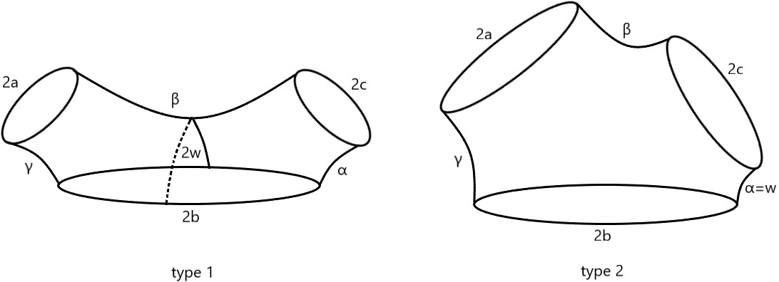
Figure 4. two types of $\mathcal{P}^{\prime}s$

One may cut the pair of pants in Figure 4 along the shortest perpendiculars between three closed boundary geodesics of $\mathcal{P}$ to get two right-angled hexagons as shown in Figure 5.

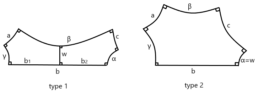
Figure 5.

Remark.

In Type-1, $2b$ is a boundary curve of $X$, and $2a,2c$ may or may not be part of the boundary. In Type-2, $2b$ and $2c$ are two boundary curves of $X$ and $2a$ may or may not be.

Construction (for $X_{\delta}$).

Now for certain $\delta>0$, we construct a new hyperbolic surface $X_{\delta}$ based on $X\in\mathcal{T}_{g,n}(x_{1},...,x_{n})$ with total boundary length reduced by $\delta$. From the discussion above, one may first find a pair of pants $\mathcal{P}\subset X$ with one boundary curve $2b$.

Case-a: $X\neq\mathcal{P}\cong S_{0,3}$. If $\mathcal{P}$ is of Type-1 as shown in Figure 4 above, let $\mathcal{P}_{\delta}$ be the pair of pants with boundary lengths $(2a,2b-\delta,2c)$. If $\mathcal{P}$ is of Type-2 as shown in Figure 4 above, let $\mathcal{P}_{\delta}$ be the pair of pants with boundary lengths $(2a,2b-\frac{1}{2}\delta,2c-\frac{1}{2}\delta)$. Then we glue $\mathcal{P}_{\delta}$ and $X\setminus\mathcal{P}$ together along the same closed geodesics and twists as those when gluing $\mathcal{P}$ and $X\setminus\mathcal{P}$ back into $X$. Hence we get a new hyperbolic surface $X_{\delta}$ with total boundary length reduced by $\delta$. In other words, we fix the part $X\setminus\mathcal{P}$ and just decrease the length of boundary $2b$ or $(2b,2c)$ to get $X_{\delta}$.

Case-b: $X=\mathcal{P}\cong S_{0,3}$. We only decrease $2b$ to $2b-\delta$ in Type-1 and decrease $(2b,2c)$ to $(2b-\frac{1}{2}\delta,2c-\frac{1}{2}\delta)$ in Type-2 as above.

That is,

$$X_{\delta}\in\mathcal{T}_{g,n}(x_{1}-\delta,x_{2},\cdots,x_{n})$$

if $\mathcal{P}$ is of Type-1 (assume $x_{1}=2b$) and

$$X_{\delta}\in\mathcal{T}_{g,n}(x_{1}-\frac{1}{2}\delta,x_{2}-\frac{1}{2}\delta,x_{3},\cdots,x_{n})$$

if $\mathcal{P}$ is of Type-2 (assume $x_{1}=2b$ and $x_{2}=2c$).

Our main task in this section is to show the following result.

Proposition 40.

There exists a constant $A_{0}>0$ only depending on $A$ such that the following hold: for any $0<\delta\leq A_{0}$ and $X\in\mathcal{T}_{g,n}(x_{1},...,x_{n})$ with $\sum x_{i}\geq n(2Am+\delta)$, the above construction for $X_{\delta}$ exists, and moreover for any filling closed curve $\eta$ in $S_{g,n}$, we have

$$\ell_{\eta}(X)-\ell_{\eta}(X_{\delta})\geq\frac{1}{2}\left(1-O_{A}(\frac{mn}{\sum x_{i}})\right)\delta.$$

Assuming Proposition 40 first, we now finish the proof of Theorem 38.

Proof of Theorem 38.

We choose $A=1$ in Proposition 40. Assume that the term $|O_{A}(\frac{mn}{\sum x_{i}})|\leq C\frac{mn}{\sum x_{i}}$ in Proposition 40 for some constant $C>0$. Take

$$L_{0}=\max\{C,2A+A_{0}\}.$$

For $0\leq\Delta\leq\sum x_{i}-L_{0}\frac{mn}{\epsilon_{1}}$, assume $\Delta=k\delta$ where $k>0$ is an integer and $0<\delta\leq A_{0}$. One may repeat the construction above in $k$ times to find a sequence of pairs of pants, reduce total boundary length for $\delta$ each time, and obtain a sequence of hyperbolic surfaces $X^{0},X^{1},\cdots,X^{k}$ where $X^{0}=X$ and $X^{j+1}=(X^{j})_{\delta}$ is the new hyperbolic surface obtained from $X^{j}$ by the construction above. Then $X^{j}$ has total boundary length equal to $\left(\sum x_{i}-j\delta\right)$. In particular

$$X^{k}\in\mathcal{T}_{g,n}(y_{1},\cdots,y_{n})$$

for some $y_{i}\leq x_{i}$ with $\sum x_{i}-\sum y_{i}=k\delta=\Delta$. We remark here that one can always apply the construction above to $X^{j}$ for each $0\leq j\leq k$ since its total boundary length $\sum x_{i}-j\delta\geq L_{0}\frac{mn}{\epsilon_{1}}\geq(2A+A_{0})mn$ which satisfies the assumption. Then it follows by Proposition 40 that for any filling closed curve $\eta$ in $S_{g,n}$ and each $0\leq j\leq k-1$,

$$\ell_{\eta}(X^{j})-\ell_{\eta}(X^{j+1})\geq\frac{1}{2}\left(1-C\frac{mn}{L_{0}mn/\epsilon_{1}}\right)\delta\geq\frac{1}{2}(1-\epsilon_{1})\delta$$

which implies that

$$\ell_{\eta}(X)-\ell_{\eta}(X^{k})\geq\frac{1}{2}(1-\epsilon_{1})\Delta.$$

Then the conclusion follows by choosing $Y=X^{k}$. ∎

Now we aim to prove Proposition 40.

We first assume the existence of $X_{\delta}$. Normally it is hard to calculate the length $\ell_{\eta}(X_{\delta})$. Instead, we construct a closed piecewise geodesic $\eta^{\prime}$ in $X_{\delta}$ homotopic to $\eta$ and then show that

$$\ell_{\eta}(X)-\ell(\eta^{\prime})\geq\frac{1}{2}\left(1-O_{A}(\frac{mn}{\sum x_{i}})\right)\delta$$

implying that

$$\ell_{\eta}(X)-\ell_{\eta}(X_{\delta})\geq\frac{1}{2}\left(1-O_{A}(\frac{mn}{\sum x_{i}})\right)\delta$$

where $\ell(\eta^{\prime})$ is the length of the closed piecewise geodesic $\eta^{\prime}$ in $X_{\delta}$, and clearly we have $\ell(\eta^{\prime})\geq\ell_{\eta}(X_{\delta})$.

Let $\eta$ be a closed filling curve in $S_{g,n}$ and still use $\eta$ to denote the corresponding closed geodesic representative in $X$. Since $\eta$ is filling, it must intersect with the pair of pants $\mathcal{P}$ for certain times if $X\neq\mathcal{P}\cong S_{0,3}$. Let’s first assume that $X$ is not $S_{0,3}$. Consider the set of all the intersection points $\eta\cap\partial\mathcal{P}$ which separates $\eta$ into several segments. Assume that

(65) $$\eta=(\cup I_{i})\cup(\cup J_{j})$$

where the $I_{i}$’s are geodesic segments in $X\setminus\mathcal{P}$ with endpoints on $\partial\mathcal{P}\cap\partial(X\setminus\mathcal{P})$, and the $J_{j}$’s are geodesic segments in $\mathcal{P}$ with endpoints on $\partial\mathcal{P}\cap\partial(X\setminus\mathcal{P})$. For each $J_{j}$, let $J^{\prime}_{j}$ be the geodesic segment representative in $\mathcal{P}_{\delta}$ (defined in the construction above) which is homotopic to $J_{j}$ in $\mathcal{P}$ (as a topological space) relative to the two endpoints of $J_{j}$. In other words, we fix the endpoints of $J_{j}$ and shrink $J_{j}$ to a shortest geodesic segment $J^{\prime}_{j}$ in $\mathcal{P}_{\delta}$. Since $X$ and $X_{\delta}$ have the same length and twist parameters for those simple closed geodesics $\partial\mathcal{P}\cap\partial(X\setminus\mathcal{P})$, replacing $\mathcal{P}$ and $J_{j}$ by $\mathcal{P}_{\delta}$ and $J_{j}^{\prime}$ respectively, we have that the closed curve

$$\eta^{\prime}=(\cup I_{i})\cup(\cup J^{\prime}_{j})\subset X_{\delta}$$

is a closed piecewise geodesic homotopic to $\eta$ and

(66) $$\ell_{\eta}(X)-\ell(\eta^{\prime})=\sum\left(\ell(J_{j})-\ell(J^{\prime}_{j})\right).$$

See Figure 6 for an example. If $X=\mathcal{P}\cong S_{0,3}$, we just denote $\eta^{\prime}$ to be the closed geodesic in $X_{\delta}$ homotopic to $\eta$. We will show that for each $j$,

(67) $$\ell(J_{j})-\ell(J^{\prime}_{j})\geq\frac{1}{2}\left(1-O_{A}(\frac{mn}{\sum x_{i}})\right)\delta.$$

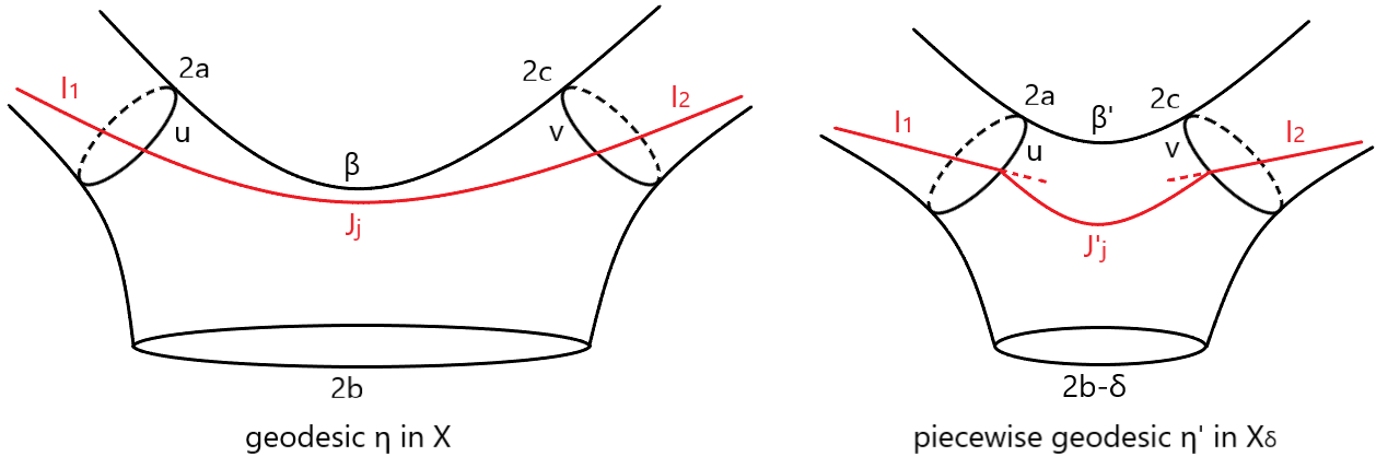
Figure 6. an example for $\eta$ and $\eta^{\prime}$

Remark.

As shown in Figure 6, we denote $u$ to be the part of geodesic $2a$ from the endpoint of $J_{j}$ to $\beta$ (the shortest geodesic between $2a$ and $2c$), and denote $v$ to be the part of geodesic $2c$ from the endpoint of $J_{j}$ to $\beta$. By saying fixing the endpoints of $J_{j}$, we just mean to keep the lengths of $u$ and $v$ to be unchanged.

Remark 41.

The existence of $J_{j}$ is the only place where we apply the assumption that $\eta$ is filling. Actually if $\eta$ is an arbitrary closed curve in $S_{g,n}$, we will show that

$$\ell_{\eta}(X)-\ell_{\eta}(X_{\delta})\geq\frac{k}{2}\left(1-O_{A}(\frac{mn}{\sum x_{i}})\right)\delta$$

where $k$ is the number of components of $\eta\cap\mathring{\mathcal{P}}$ where $\mathring{\mathcal{P}}$ is the interior of $\mathcal{P}$.

To prove (67), we separate $J_{j}$ into several pieces. In the universal covering space of the pair of pants $\mathcal{P}$, $J_{j}$ is lifted onto a simple geodesic segment with endpoints on the boundary. See Figure 7 for an example.

Figure 7. an example for $\eta$ in $\mathcal{P}$

Now we split the proof of Proposition 40 into the following subsections.

8.1. A technical lemma for deforming pairs of pants

First we recall the following formulas for hyperbolic distance, which one may refer to [Bus92, Formula Glossary and (2.3.2)].

Lemma 42.

In the right-angled hexagon in Figure 8, we have

$$\cosh c=\sinh a\sinh b\cosh\gamma-\cosh a\cosh b,$$

$$\frac{\sinh\alpha}{\sinh a}=\frac{\sinh\beta}{\sinh b}=\frac{\sinh\gamma}{\sinh c}.$$

In the right-angled pentagon in Figure 8, we have

$$\cosh c=\sinh a\sinh b.$$

In the rectangle with right angle between $x,a$ and right angle between $y,a$ in Figure 8, we have

$$\cosh\alpha=\cosh x\cosh y\cosh a-\sinh x\sinh y.$$

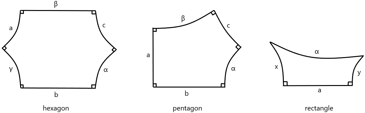
Figure 8.

Remark.

In the rectangle case above, the same formula still holds when $x$ or $y$ may be negative. Where for $x\cdot y<0$, it means that the edges $x$ and $y$ are on the different sides of $a$. In this case $\alpha$ will intersect with $a$.

In the rectangle case above, we provide the following technical lemma which will be repeatedly applied later.

Lemma 43.

In the rectangle as shown in Figure 8 above, assume that $a,x,y$ and $\alpha$ are smooth functions parametrized on the same domain by the variable $t$. Then we have

$$\left|\dot{\alpha}\tanh\alpha-\dot{a}\tanh a-\dot{x}\tanh x-\dot{y}\tanh y\right|$$

$$\leq \frac{1}{\cosh a-1}\left(|\dot{a}|\tanh a+\frac{|\dot{x}|}{\cosh^{2}x}+\frac{|\dot{y}|}{\cosh^{2}y}\right).$$

In particular, if $\alpha\geq a\geq C$ for some constant $C>0$, then we have

$$\left|\dot{\alpha}-\dot{a}\right|\leq C^{\prime}_{C}\cdot\left(e^{-a}|\dot{a}|+|\dot{x}|+|\dot{y}|\right)$$

for some constant $C^{\prime}_{C}>0$ only depending on $C$.

Proof.

By Lemma 42 we have

$$\cosh\alpha = \cosh x\cosh y\cosh a-\sinh x\sinh y$$

$$= \cosh x\cosh y(\cosh a-1)+\cosh(x-y).$$

Taking derivative we have

$$\frac{\sinh\alpha}{\cosh\alpha}\dot{\alpha} = \dot{a}\frac{\cosh x\cosh y\sinh a}{\cosh\alpha}$$

$$+\dot{x}\frac{\sinh x\cosh y(\cosh a-1)}{\cosh\alpha}$$

$$+\dot{y}\frac{\cosh x\sinh y(\cosh a-1)}{\cosh\alpha}$$

$$+(\dot{x}-\dot{y})\frac{\sinh(x-y)}{\cosh\alpha}$$

$$= \dot{a}\frac{\cosh x\cosh y\sinh a}{\cosh\alpha}$$

$$+\dot{x}\frac{\sinh x\cosh y\cosh a-\cosh x\sinh y}{\cosh\alpha}$$

$$+\dot{y}\frac{\cosh x\sinh y\cosh a-\sinh x\cosh y}{\cosh\alpha}.$$

Now we estimate the difference. From (8.1), we have

$$\left|\frac{\cosh x\cosh y\sinh a}{\cosh\alpha}-\frac{\sinh a}{\cosh a}\right|$$

$$= \frac{\tanh a\sinh x\sinh y}{\cosh\alpha}$$

$$\leq \frac{\tanh a}{\cosh a-1},$$

$$\left|\frac{\sinh x\cosh y\cosh a-\cosh x\sinh y}{\cosh\alpha}-\frac{\sinh x}{\cosh x}\right|$$

$$= \frac{\sinh y}{\cosh x\cosh\alpha}$$

$$\leq \frac{1}{\cosh^{2}x(\cosh a-1)},$$

and

$$\left|\frac{\cosh x\sinh y\cosh a-\sinh x\cosh y}{\cosh\alpha}-\frac{\sinh y}{\cosh y}\right|$$

$$= \frac{\sinh x}{\cosh y\cosh\alpha}$$

$$\leq \frac{1}{\cosh^{2}y(\cosh a-1)}.$$

Put all the inequalities above together we get

$$|\dot{\alpha}\tanh\alpha-\dot{a}\tanh a-\dot{x}\tanh x-\dot{y}\tanh y|$$

$$\leq \frac{1}{\cosh a-1}(|\dot{a}|\tanh a+\frac{|\dot{x}|}{\cosh^{2}x}+\frac{|\dot{y}|}{\cosh^{2}y})$$

which completes the proof of the first part.

The second part follows by the first part:

$$|\dot{\alpha}\tanh\alpha-\dot{a}\tanh a| \leq |\dot{\alpha}\tanh\alpha-\dot{a}\tanh a-\dot{x}\tanh x-\dot{y}\tanh y|$$

$$+|\dot{x}\tanh x|+|\dot{y}\tanh y|$$

$$\leq \frac{|\dot{a}|+|\dot{x}|+|\dot{y}|}{\cosh a-1}+|\dot{x}|+|\dot{y}|$$

$$= \frac{|\dot{a}|}{\cosh a-1}+(|\dot{x}|+|\dot{y}|)\cdot\frac{\cosh a}{\cosh a-1}.$$

Since $\alpha\geq a\geq C$, we have

$$|\dot{\alpha}-\dot{a}| \leq \frac{1}{\tanh\alpha}|\dot{\alpha}\tanh\alpha-\dot{a}\tanh a|+|\dot{a}(1-\frac{\tanh a}{\tanh\alpha})|$$

$$\leq \frac{|\dot{a}|}{\tanh a(\cosh a-1)}+\frac{(|\dot{x}|+|\dot{y}|)\cosh a}{\tanh a(\cosh a-1)}+|\dot{a}|(1-\tanh a)$$

$$\leq C^{\prime}_{C}\left(e^{-a}|\dot{a}|+|\dot{x}|+|\dot{y}|\right)$$

for some constant $C^{\prime}_{C}>0$ only depending on $C$. ∎

Next we will prove Proposition 40 for Type-1 and Type-2 separately in the following two subsections.

8.2. Proof of Proposition 40 for Type-1

Now we consider a pair of pants in Figure 4 of Type-1 and the corresponding right-angled hexagon in Figure 5 of Type-1.

In this subsection, we always use the notation $w$ to be the perpendicular between $b$ and $\beta$ in Figure 5 of Type-1. For the pants $\mathcal{P}$ of Type-1 we construct, (64) holds. But when reducing $b$, the number $w$ may increase such that (64) does not hold again. Instead, we always assume $w$ satisfies

(73) $$\sinh w\leq 2\pi\frac{m}{b}.$$

Later in the proof of Proposition 51 we will show (73) always holds when $b$ does not reduce too much.

Let $b_{1},b_{2}>0$ as shown in Figure 5. By Lemma 42 we have

$$\cosh a=\sinh b_{1}\sinh w$$

and

$$\cosh c=\sinh b_{2}\sinh w.$$

So we have

$$\cosh a\cosh c = \sinh^{2}w\sinh b_{1}\sinh b_{2}$$

$$= \frac{1}{2}\sinh^{2}w(\cosh(b_{1}+b_{2})-\cosh(b_{1}-b_{2}))$$

$$\leq \frac{1}{2}\sinh^{2}w\cosh b.$$

Now we consider reducing the length of boundary $2b$ of $\mathcal{P}$. Let $\{a(t),b(t),c(t)\}$ be the length functions in terms of a common parameter $t$. In our process from $\mathcal{P}$ to $\mathcal{P}_{\delta}$, we assume $a$ and $c$ are fixed and $b$ decreases with constant speed. More precisely, denote $\dot{b}=\frac{db}{dt}$ and assume

(75) $$\dot{a}=\dot{c}=0\quad\emph{and}\quad\dot{b}=-1.$$

As shown in Figure 4, in the pair of pants with boundary length $(2a,2b,2c)$, we always denote $\alpha$ to be the shortest perpendicular between $2b$ and $2c$, denote $\beta$ to be the shortest perpendicular between $2a$ and $2c$, and denote $\gamma$ to be the shortest perpendicular between $2a$ and $2b$. One may also see Figure 8 for the corresponding hexagon. Then by Lemma 42, we have

(76) $$\cosh\alpha=\frac{\cosh a+\cosh b\cosh c}{\sinh b\sinh c},$$

(77) $$\cosh\gamma=\frac{\cosh c+\cosh a\cosh b}{\sinh a\sinh b},$$

(78) $$\cosh\beta=\frac{\cosh b+\cosh a\cosh c}{\sinh a\sinh c},$$

and

(79) $$\cosh w=\sinh c\sinh\alpha=\sinh a\sinh\gamma.$$

A direct computation shows that

$$\dot{\alpha} = \frac{1}{\sinh\alpha}\frac{\cosh c+\cosh a\cosh b}{\sinh^{2}b\sinh c}$$

$$= \frac{1}{\cosh w}\frac{\cosh c+\cosh a\cosh b}{\sinh^{2}b},$$

$$\dot{\gamma} = \frac{1}{\sinh\gamma}\frac{\cosh a+\cosh b\cosh c}{\sinh^{2}b\sinh a}$$

$$= \frac{1}{\cosh w}\frac{\cosh a+\cosh b\cosh c}{\sinh^{2}b},$$

and

$$\dot{\beta} = -\frac{1}{\sinh\beta}\frac{\sinh b}{\sinh a\sinh c}$$

$$= -\frac{\cosh\beta}{\sinh\beta}\frac{\sinh b}{\cosh b+\cosh a\cosh c}.$$

A direct consequence of all the equations above is

Lemma 44.

If $b\geq Am$ and (73) holds, then we have

1. $0<\dot{\alpha}=O_{A}\left(\frac{m^{2}}{b^{2}}\right)$ and $0<\dot{\gamma}=O_{A}\left(\frac{m^{2}}{b^{2}}\right)$.

2. $\cosh\beta\geq 1+\frac{1}{2\pi^{2}}\frac{b^{2}}{m^{2}}$, $\dot{\beta}<0$ and $|\dot{\beta}+1|=O_{A}\left(\frac{m^{2}}{b^{2}}\right)$.

Proof.

For Part $(1)$, clearly we have $0<\dot{\alpha}$ and $0<\dot{\gamma}$. By (8.2) and (8.2) we have

$$\dot{\alpha} \leq \frac{2}{\cosh w}\frac{\cosh c\cosh a\cosh b}{\sinh^{2}b}$$

$$\leq \frac{\sinh^{2}w}{\cosh w}\frac{\cosh^{2}b}{\sinh^{2}b}$$

$$\leq \frac{1}{\tanh^{2}A}4\pi^{2}\frac{m^{2}}{b^{2}}$$

where in the last inequality we apply $b\geq Am\geq A$, $\cosh w\geq 1$ and (73). By a similar argument one may also show

$$\dot{\gamma}\leq\frac{1}{\tanh^{2}A}4\pi^{2}\frac{m^{2}}{b^{2}}.$$

For Part $(2)$, clearly we have $\dot{\beta}<0$. By (73), (8.2) and (78) we have

$$\cosh\beta \geq \frac{\cosh b}{\cosh a\cosh c}+1$$

$$\geq \frac{2}{\sinh^{2}w}+1$$

$$\geq 1+\frac{1}{2\pi^{2}}\frac{b^{2}}{m^{2}}.$$

In particular $e^{\beta}>\frac{1}{2\pi^{2}}\frac{b^{2}}{m^{2}}\geq\frac{A}{2\pi^{2}}$. Then by (8.2) and (8.2) we have

$$|\dot{\beta}+1| = \left|1-\frac{\tanh b}{\tanh\beta}\frac{1}{1+\frac{\cosh a\cosh c}{\cosh b}}\right|$$

$$\leq \left|1-\frac{1}{1+\frac{\cosh a\cosh c}{\cosh b}}\right|+\left|1-\frac{\tanh b}{\tanh\beta}\right|\frac{1}{1+\frac{\cosh a\cosh c}{\cosh b}}$$

$$\leq \frac{\cosh a\cosh c}{\cosh b}+\left|1-\frac{\tanh b}{\tanh\beta}\right|$$

$$\leq \frac{1}{2}\sinh^{2}w+\frac{|\sinh(\beta-b)|}{\sinh\beta\cosh b}.$$

Since $b\geq mA\geq A$, $\frac{|\sinh(\beta-b)|}{\sinh\beta\cosh b}=O_{A}\left(e^{-2\beta}+e^{-2b}\right)$. Thus, by (73) we obtain

$$|\dot{\beta}+1| \leq 2\pi^{2}\frac{m^{2}}{b^{2}}+O_{A}\left(e^{-2\beta}+e^{-2b}\right)$$

$$\leq O_{A}\left(\frac{m^{2}}{b^{2}}\right)$$

as desired. ∎

Let $J_{j}\subset\mathcal{P}$ be a geodesic segment in (65). We classify $J_{j}$ in terms of its possible intersections with $\alpha,\gamma,a$ and $c$ (without orientation). Actually we have

Lemma 45.

There are 14 kinds of possible segments as shown in Figure 9 where each one is a fundamental domain for $\mathcal{P}$ (or half of a fundamental domain). More precisely, they are: from $\alpha$ to $\gamma$ (type 1.1, 1.2), from $\alpha$ to $\alpha$ (type 1.4), from $\gamma$ to $\gamma$ (type 1.3), from $a$ to $\alpha$ (type 1.5, 1.6), from $a$ to $\gamma$ (type 1.9, 1.10), from $c$ to $\gamma$ (type 1.7, 1.8), from $c$ to $\alpha$ (type 1.11, 1.12) and from $a$ to $c$ (type 1.13, 1.14).

We denote $d$ as the geodesic segment of $J_{j}$ in each kind.

If $J_{j}$ intersects with a piece of $\alpha$, we denote $p$ to be the intersection point and $x$ to be the half segment of $\alpha$ that goes from $p$ to $c$: for this case, see types $1.1,1.2,1.4,1.5,1.6,1.11$ and $1.12$ as shown in Figure 9. If $J_{j}$ intersects with a piece of $\gamma$, denote $q$ to be the intersection point and $y$ to be the half segment of $\gamma$ that goes from $q$ to $a$: see types $1.1,1.2,1.3,1.7,1.8,1.9$ and $1.10$ as shown in Figure 9. If $J_{j}$ does not intersect with any piece of $\alpha$ and $\gamma$, see types $1.13$ and $1.14$ as shown in Figure 9. We fix these points $\{p,q\}$ as $b$ decreases, that is, we keep the length of $x$ and $y$ to be unchanged as $b$ decreases. We remark here that by Lemma 44 both $\alpha$ and $\gamma$ increase as $b$ decreases. So the points $p$ and $q$ still lie in $\alpha$ and $\gamma$ respectively during the process.

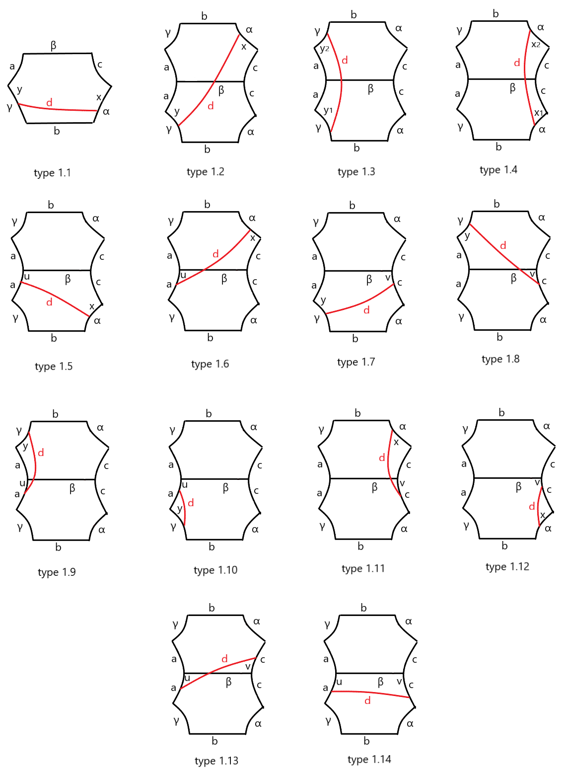
Figure 9. $14$ kinds of geodesic segments in Type-1

These intersection points separate $J_{j}$ into several segments. Fixing these points as $b$ is decreasing, then we get a piecewise geodesic $J^{\prime\prime}_{j}$ homotopic to $J_{j}$ in $\mathcal{P}_{\delta}$.

In types 1.3 and 1.4, the lengths $a,y_{1},y_{2},c,x_{1}$ and $x_{2}$ are unchanged during the process, so the corresponding $d$ is unchanged. In types 1.9, 1.10, 1.11 and 1.12, the endpoints of $J_{j}$ on boundary curves $2a$ and $2c$ are fixed, so the lengths $u$ and $v$, which are segments on $a$ and $c$ from the endpoint of $J_{j}$ to $\beta$ respectively (see Figure 6), in the figure are also unchanged. Also, since $a,y,c$ and $x$ are unchanged, the corresponding $d$ is also unchanged.

For the remaining $8$ kinds, we will show that

(83) $$|\dot{d}+1|=O_{A}\left(\frac{m^{2}}{b^{2}}\right)$$

and $J_{j}$ must contain at least one of those $8$ kinds.

Lemma 46.

The segment $J_{j}$ for Type-1 must contain at least one segment of types 1.1, 1.2, 1.5, 1.6, 1.7, 1.8, 1.13 and 1.14 as shown in Figure 9.

Proof.

If $X=\mathcal{P}\cong S_{0,3}$, then $\eta$ is a single $J$ and does not intersect with $2a$ and $2c$. So it is a combination of types $1.1,1.2,1.3$, and $1.4$. Since $\eta$ is a filling closed curve, it must intersect with $\alpha$ and $\gamma$. So $\eta$ contains at least one segment from $\alpha$ to $\gamma$, that is of type 1.1 or 1.2.

If $X$ is not $S_{0,3}$, then $\eta$ must intersect with at least one of $2a$ and $2c$, and thus $J_{j}$ must have an endpoint on $a$ or $c$. Suppose $J_{j}$ do not contain any of types $1.1,1.2,1.5,1.6,1.7,1.8,1.13$ and $1.14$. Then $J_{j}$ only consists of segments which may be from $a$ to $\gamma$, or from $\gamma$ to $\gamma$, or from $c$ to $\alpha$ and or from $\alpha$ to $\alpha$. So if starting at a point on $a$, the geodesic $J_{j}$ can only travel to $\gamma$, then go to next $\gamma$ several times, and finally return to $a$. But in this way $J_{j}$ would be homotopic to a piece of geodesic line $a$, which contradicts to the assumption that $J_{j}$ is part of a shortest closed geodesic representative for $\eta$ as shown in (65). Similarly the geodesic $J_{j}$ can not start at a point in $c$. So $J_{j}$ must contain at least one segment of those 8 kinds. ∎

Next we prove (83) for those $8$ types in Lemma 46 case by case.

Lemma 47 (type 1.1).

If $b\geq Am$ and (73) holds, then for type 1.1 in Figure 9 we have

$$|\dot{d}+1|=O_{A}\left(\frac{m^{2}}{b^{2}}\right).$$

Proof.

Recall that $\dot{x}=\dot{y}=0$ and $\dot{b}=-1$. Since $b\geq Am$ and (73) holds, it follows by Lemma 44 that $|\dot{\alpha}|=O_{A}\left(\frac{m^{2}}{b^{2}}\right)$ and $|\dot{\gamma}|=O_{A}\left(\frac{m^{2}}{b^{2}}\right)$. It is clear that $e^{-b}\leq\frac{2}{b^{2}}$. Next we apply Lemma 43 to the rectangle $(\gamma-y,b,\alpha-x,d)$ to get

$$|\dot{d}+1|=|\dot{d}-\dot{b}|\leq A^{\prime}(e^{-b}+|\dot{\alpha}|+|\dot{\gamma}|)=O_{A}\left(\frac{m^{2}}{b^{2}}\right)$$

for some constant $A^{\prime}>0$ only depending on $A$. ∎

Lemma 48 (type 1.2).

If $b\geq Am$ and (73) holds, then for type 1.2 in Figure 9 we have

$$|\dot{d}+1|=O_{A}\left(\frac{m^{2}}{b^{2}}\right).$$

Proof.

Let $h$ be the perpendicular between $\alpha$ and $\gamma$ in type 1.2. Let $e$ to be part of $\alpha$ between $h$ and $b$, and let $f$ to be part of $\gamma$ between $h$ and $a$ (see Figure 10). Then we have a rectangle $(\alpha-e-x,h,y-f,d)$ with $\angle(h,\alpha-e-x)=\angle(h,y-f)=\frac{\pi}{2}$. We remark here that the length $\alpha-e-x$ and $y-f$ may be negative. Now we compute the lengths of these edges and their derivatives.

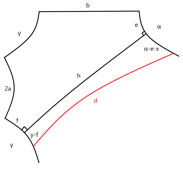
Figure 10.

By Lemma 42 and (77) we have

$$\cosh h = \sinh 2a\sinh b\cosh\gamma-\cosh 2a\cosh b$$

$$= 2\sinh a\cosh a\sinh b\frac{\cosh c+\cosh a\cosh b}{\sinh a\sinh b}$$

$$-(2\cosh^{2}a-1)\cosh b$$

$$= 2\cosh a\cosh c+\cosh b$$

and

$$\dot{h} = \dot{b}\frac{\sinh b}{\sinh h}$$

$$= \dot{b}\frac{\cosh h}{\sinh h}\frac{\sinh b}{2\cosh a\cosh c+\cosh b}.$$

So by (73), (8.2), $h\geq b\geq A$ and $\dot{b}=-1$, we have

$$|\dot{h}+1| = \left|1-\frac{\cosh h}{\sinh h}\frac{\sinh b}{2\cosh a\cosh c+\cosh b}\right|$$

$$\leq \left|1-\frac{\sinh b}{2\cosh a\cosh c+\cosh b}\right|+\left|1-\frac{\cosh h}{\sinh h}\right|\frac{\sinh b}{2\cosh a\cosh c+\cosh b}$$

$$\leq \frac{2\frac{\cosh a\cosh c}{\cosh b}+\frac{e^{-b}}{\cosh b}}{2\frac{\cosh a\cosh c}{\cosh b}+1}+\left(\frac{\cosh b}{\sinh b}-1\right)$$

$$\leq 4\pi^{2}\frac{m^{2}}{b^{2}}+e^{-b}+\frac{e^{-b}}{\sinh A}$$

$$= O_{A}\left(\frac{m^{2}}{b^{2}}\right).$$

By Lemma 42, (77), (79), (8.2) and (8.2) we have

$$\sinh e = \sinh 2a\frac{\sinh\gamma}{\sinh h}$$

$$= \frac{2\cosh w\cosh a}{\sinh h}$$

and

$$\quad\ \dot{e} = \frac{1}{\cosh e}\sinh 2a\bigg{(}\dot{\gamma}\frac{\cosh\gamma}{\sinh h}-\dot{h}\frac{\sinh\gamma\cosh h}{\sinh^{2}h}\bigg{)}$$

$$= \frac{\sinh 2a}{\cosh e}\bigg{[}\frac{1}{\cosh w}\frac{(\cosh a+\cosh b\cosh c)}{\sinh^{2}b}\frac{(\cosh c+\cosh a\cosh b)}{\sinh a\sinh b\sinh h}$$

$$+\frac{\sinh b}{\sinh h}\frac{\cosh w}{\sinh a}\frac{\cosh h}{\sinh^{2}h}\bigg{]}$$

$$= \frac{1}{\cosh e}\bigg{[}\frac{2\cosh a}{\cosh w}\frac{(\cosh a+\cosh b\cosh c)}{\sinh^{2}b}\frac{(\cosh c+\cosh a\cosh b)}{\sinh b\sinh h}$$

$$+2\frac{\cosh a}{\sinh h}\frac{\sinh b}{\sinh h}\cosh w\frac{\cosh h}{\sinh h}\bigg{]}.$$

Since $h>b\geq Am$, by (73) and (8.2) it is not hard to see that $\frac{\cosh a}{\sinh h}=O_{A}\left(\frac{m^{2}}{b^{2}}\right)$ and $\frac{2\cosh a}{\cosh w}\frac{(\cosh a+\cosh b\cosh c)}{\sinh^{2}b}\frac{(\cosh c+\cosh a\cosh b)}{\sinh b\sinh h}=O_{A}\left(\frac{m^{4}}{b^{4}}\right)$. Recall that by (73) $\cosh w=\sqrt{\sinh^{2}w+1}\leq\sqrt{4\pi^{2}\frac{m^{2}}{b^{2}}+1}\leq\sqrt{\frac{4\pi^{2}}{A^{2}}+1}$. So we have that $e\leq\sinh e=O_{A}\left(\frac{m^{2}}{b^{2}}\right)$ and $0\leq\dot{e}=O_{A}\left(\frac{m^{2}}{b^{2}}\right)$.

By Lemma 42, (8.2) and (8.2) we have

(88) $$\sinh f=\sinh b\frac{\sinh\gamma}{\sinh h}$$

and

$$\quad\quad\dot{f} = \frac{1}{\cosh f}\bigg{(}\dot{\gamma}\cosh\gamma\frac{\sinh b}{\sinh h}+\dot{b}\sinh\gamma\frac{\cosh b}{\sinh h}-\dot{h}\sinh\gamma\frac{\sinh b\cosh h}{\sinh^{2}h}\bigg{)}$$

$$= \dot{\gamma}\frac{\cosh\gamma}{\cosh f}\frac{\sinh b}{\sinh h}+\dot{b}\frac{\sinh\gamma}{\cosh f}\bigg{(}\frac{\cosh b}{\sinh h}-\frac{\sinh^{2}b\cosh h}{\sinh^{3}h}\bigg{)}$$

$$= \dot{\gamma}\frac{\cosh\gamma}{\cosh f}\frac{\sinh b}{\sinh h}+\dot{b}\frac{\sinh\gamma}{\cosh f}\frac{(\cosh h-\cosh b)(1+\cosh b\cosh h)}{\sinh^{3}h}$$

$$= \dot{\gamma}\frac{\cosh\gamma}{\cosh f}\frac{\sinh b}{\sinh h}-\frac{\sinh\gamma}{\cosh f}\frac{2\cosh a\cosh c(1+\cosh b\cosh h)}{\sinh^{3}h}.$$

Since $\frac{\sinh\gamma}{\sinh f}=\frac{\sinh h}{\sinh b}\leq\frac{2\cosh a\cosh c+\cosh b}{\sinh b}=O_{A}(1)$ is bounded (by (8.2) and (8.2)), we know that $\frac{\cosh\gamma}{\cosh f}=O_{A}(1)$ is also bounded. Apply (73) and (8.2) and the fact that $h>b\geq Am$, we have that $\frac{2\cosh a\cosh c(1+\cosh b\cosh h)}{\sinh^{3}h}=O_{A}\left(\frac{m^{2}}{b^{2}}\right)$. Thus together with Lemma 44, we have $|\dot{f}|=O_{A}\left(\frac{m^{2}}{b^{2}}\right)$.

Now consider the rectangle $(\alpha-e-x,h,y-f,d)$. By Lemma 44 and the discussion above we have $|\dot{\alpha}-\dot{e}|=O_{A}\left(\frac{m^{2}}{b^{2}}\right)$, $|\dot{f}|=O_{A}\left(\frac{m^{2}}{b^{2}}\right)$ and $|\dot{h}+1|=O_{A}\left(\frac{m^{2}}{b^{2}}\right)$. Recall that $\dot{x}=\dot{y}=0$ and $h>b\geq Am$. Then we apply Lemma 43 to the rectangle $(\alpha-e-x,h,y-f,d)$ to get $|\dot{d}+1|=O_{A}\left(\frac{m^{2}}{b^{2}}\right)$ as desired. ∎

Lemma 49 (types 1.5–1.8).

If $b\geq Am$ and (73) holds, then for types 1.5, 1.6, 1.7 and 1.8 in Figure 9 we have

$$|\dot{d}+1|=O_{A}\left(\frac{m^{2}}{b^{2}}\right).$$

Proof.

We only prove the lemma for type 1.5. For the other three types, the proofs are similar as the one for type 1.5.

Let $h$ be the perpendicular between $a$ and $\alpha$ in type 1.5. Let $e$ to be part of $\alpha$ between $h$ and $b$, and let $f$ to be part of $a$ between $h$ and $\gamma$ (see Figure 11). Then we have a rectangle $(f+u-a,h,e+x-\alpha,d)$ with $\angle(h,f+u-a)=\angle(h,e+x-\alpha)=\frac{\pi}{2}$. We remark here that the length $f+u-a$ and $e+x-\alpha$ may be negative. Now we compute the lengths of these edges and their derivatives.

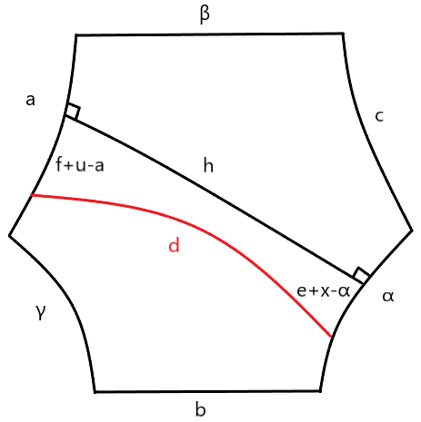
Figure 11.

By Lemma 42, (77), (79) and (8.2), we have

$$\cosh h = \sinh b\sinh\gamma$$

$$= \frac{\cosh w}{\sinh a}\sinh b$$

and

$$\quad\quad\dot{h} = \frac{1}{\sinh h}\bigg{(}\dot{b}\cosh b\sinh\gamma+\dot{\gamma}\sinh b\cosh\gamma\bigg{)}$$

$$= -\frac{\cosh h}{\sinh h}\frac{\cosh b}{\sinh b}$$

$$+\frac{1}{\cosh w}\frac{(\cosh a+\cosh b\cosh c)}{\sinh^{2}b}\frac{(\cosh c+\cosh a\cosh b)}{\sinh a\sinh b}\frac{\sinh b}{\sinh h}$$

$$= -\frac{\cosh h}{\sinh h}\frac{\cosh b}{\sinh b}$$

$$+\frac{1}{\cosh^{2}w}\frac{\cosh h}{\sinh h}\frac{(\cosh a+\cosh b\cosh c)(\cosh c+\cosh a\cosh b)}{\sinh^{3}b}.$$

Since $b\geq Am$, by (73), (8.2) and (8.2) it is easy to see that $\frac{1}{\cosh h}=O_{A}\left(\frac{m^{2}}{b^{2}}\right)$. Which also implies that $|\frac{\cosh h}{\sinh h}\frac{\cosh b}{\sinh b}-1|=O_{A}\left(\frac{m^{4}}{b^{4}}\right)$. Then by (73) and (8.2) it is not hard to see that

$$\frac{1}{\cosh^{2}w}\frac{\cosh h}{\sinh h}\frac{(\cosh a+\cosh b\cosh c)(\cosh c+\cosh a\cosh b)}{\sinh^{3}b}=O_{A}\left(\frac{m^{2}}{b^{2}}\right).$$

Thus, we have

$$|\dot{h}+1|=O_{A}\left(\frac{m^{2}}{b^{2}}\right).$$

By Lemma 42, we have

$$\sinh(a-f) = \frac{\cosh c}{\sinh h}$$

$$= \frac{\cosh h}{\sinh h}\frac{1}{\cosh w}\frac{\sinh a\cosh c}{\sinh b}$$

and

$$-\dot{f} = -\dot{h}\frac{1}{\cosh(a-f)}\frac{\cosh c\cosh h}{\sinh^{2}h}$$

$$= -\dot{h}\frac{1}{\cosh(a-f)}\frac{\cosh h}{\sinh h}\sinh(a-f).$$

Then again by (73), (8.2) and the bounds for $h$ and $\dot{h}$ above, it is easy to see that

$$|a-f|=O_{A}\left(\frac{m^{2}}{b^{2}}\right)\quad\text{and}\quad|\dot{f}|=O_{A}\left(\frac{m^{2}}{b^{2}}\right).$$

By Lemma 42, we have

(94) $$\sinh e=\frac{\cosh f}{\sinh b}\leq\frac{\cosh a}{\sinh b}$$

and

$$\dot{e}=\frac{1}{\cosh e}\bigg{(}\dot{f}\frac{\sinh f}{\sinh b}-\dot{b}\frac{\cosh f\cosh b}{\sinh^{2}b}\bigg{)}$$

implying that

(95) $$|\dot{e}|\leq|\dot{f}|\frac{\sinh a}{\sinh b}+\frac{\cosh a\cosh b}{\sinh^{2}b}.$$

Then by (73) and (8.2) we have $e=O_{A}\left(\frac{m^{2}}{b^{2}}\right)$ and $|\dot{e}|=O_{A}\left(\frac{m^{2}}{b^{2}}\right).$

Recall that $\dot{u}=\dot{a}=\dot{x}=0$. Then we apply Lemma 43, Lemma 44 and all these bounds above to rectangle $(f+u-a,h,e+x-\alpha,d)$ to obtain $|\dot{d}+1|=O_{A}\left(\frac{m^{2}}{b^{2}}\right)$ as desired. ∎

Lemma 50 (types 1.13 and 1.14).

If $b\geq Am$ and (73) holds, then for types 1.13 and 1.14 in Figure 9 we have

$$|\dot{d}+1|=O_{A}\left(\frac{m^{2}}{b^{2}}\right).$$

Proof.

Recall that $\dot{u}=\dot{v}=0$. For type 1.13, by Lemma 44 and applying Lemma 43 to rectangle $(u,\beta,v,d)$, we obtain $|\dot{d}+1|=O_{A}\left(\frac{m^{2}}{b^{2}}\right)$ as desired. For type 1.14, the proof is similar. ∎

Now we are ready to prove Proposition 40 for Type-1.

Proposition 51.

Proposition 40 holds for the case that $\mathcal{P}$ is of Type-1.

Proof.

Let $2b$ to be the longest boundary geodesic of $X$, and $\mathcal{P}$ be the pants with three boundary geodesics $(2a,2b,2c)$. Since $\sum x_{i}\geq n(2Am+\delta)$, we know $2b\geq 2Am+\delta>\delta$. Hence both the pants $\mathcal{P}_{\delta}$ and the surface $X_{\delta}$ exist.

As $b$ smoothly decreases to $b-\frac{1}{2}\delta$, we denote $b^{\prime}$ and $w^{\prime}$ to be the quantities corresponding to $b$ and $w$ respectively. The lengths $a$ and $c$ are unchanged. It is clear that

$$b-\frac{1}{2}\delta\leq b^{\prime}\leq b.$$

So $b^{\prime}\geq Am$ always holds.

By Lemma 42, we have $\cosh w=\sinh c\sinh\alpha$ and then

$$\sinh^{2}w = \cosh^{2}w-1$$

$$= \sinh^{2}c\cosh^{2}\alpha-\cosh^{2}c$$

$$= \sinh^{2}c\frac{(\cosh a+\cosh b\cosh c)^{2}}{\sinh^{2}b\sinh^{2}c}-\cosh^{2}c$$

$$= \frac{\cosh^{2}a+\cosh^{2}c+2\cosh a\cosh b\cosh c}{\sinh^{2}b}.$$

Recall that $b-\frac{1}{2}\delta\leq b^{\prime}\leq b.$ Then we have

$$\frac{\sinh w^{\prime}}{\sinh w} = \frac{\sinh b}{\sinh b^{\prime}}\left(\frac{\cosh^{2}a+\cosh^{2}c+2\cosh a\cosh b^{\prime}\cosh c}{\cosh^{2}a+\cosh^{2}c+2\cosh a\cosh b\cosh c}\right)^{\frac{1}{2}}$$

$$\leq \frac{\sinh b}{\sinh(b-\frac{1}{2}\delta)}$$

$$= \cosh\frac{1}{2}\delta+\frac{1}{\tanh(b-\frac{1}{2}\delta)}\sinh\frac{1}{2}\delta$$

$$\leq \cosh\frac{1}{2}\delta+\frac{1}{\tanh A}\sinh\frac{1}{2}\delta$$

$$< 2$$

for $\delta\in(0,A_{0}]$ where $A_{0}$ is some constant only depending on $A$. Recall that (64) says that $\sinh w\leq\frac{\pi m}{b}$. So we have that for $0<\delta\leq A_{0}$, the inequality that $\sinh w^{\prime}\leq\frac{2\pi m}{b}$ always holds, i.e, equation(73) always holds. Thus the assumptions in Lemma 47, 48, 49 and 50 are always satisfied.

As the boundary length $b$ reduces by $\frac{1}{2}\delta$, the length $d$ in types 1.3, 1,4, 1.9, 1.10, 1.11 and 1.12 are unchanged. For remaining types 1.1, 1.2, 1.5, 1.6, 1.7, 1.8, 1.13 and 1.14, it follows by Lemma 47, 48, 49 and 50 that the length $d$ decreases at least $\frac{1}{2}\left(1-O_{A}\left(\frac{m^{2}}{b^{2}}\right)\right)\delta$. By Lemma 46 $J_{j}$ must contain at least one of the decreasing types. So we have

$$\ell(J_{j})-\ell(J^{\prime}_{j})\geq\frac{1}{2}\left(1-O_{A}\left(\frac{m^{2}}{b^{2}}\right)\right)\delta$$

which together with (66) imply that

$$\ell_{\eta}(X)-\ell_{\eta}(X_{\delta})\geq\frac{1}{2}\left(1-O_{A}\left(\frac{m^{2}}{b^{2}}\right)\right)\delta=\frac{1}{2}\left(1-O_{A}\left(\frac{m^{2}n^{2}}{(\sum x_{i})^{2}}\right)\right)\delta$$

where in the last equation we apply $2b\geq\frac{\sum x_{i}}{n}$.

The proof is complete. ∎

Remark.

Moreover, if $g=n=1$, then the pair of pants $\mathcal{P}$ must be of Type-1, and the two boundary curves $2a=2c$ in $\mathcal{P}$. It is not hard to see that any closed filling curve $\eta$ contains at least two decreasing types. For this case, actually one can improve Proposition 40 and Theorem 4 to be

Proposition 52.

With the same assumptions in Proposition 40, if $g=n=1$ and $X\in\mathcal{T}_{1,1}(x)$, we have

$$\ell_{\eta}(X)-\ell_{\eta}(X_{\delta})\geq\left(1-O_{A}\left(\frac{1}{x^{2}}\right)\right)\delta.$$

Theorem 53.

For any $\epsilon_{1}>0$, there exists a constant $c(\epsilon_{1})>0$ only depending on $\epsilon_{1}$ such that for all $T>0$ and any compact hyperbolic surface $X\cong S_{1,1}$ of geodesic boundary, we have

$$\#_{f}(X,T)\leq c(\epsilon_{1})\cdot e^{T-(1-\epsilon_{1})\ell(\partial X)}.$$

In this paper the bound in Proposition 40 is sufficient for us to prove Theorem 1 and 2.

8.3. Proof of Proposition 40 for Type-2

Now we consider a pair of pants in Figure 4 of Type-2 and the corresponding right-angled hexagon in Figure 5 of Type-2. Both $2b$ and $2c$ are two boundary geodesics of the surface.

In this subsection, we always use the notation $\alpha=w$ to denote the perpendicular between $b$ and $c$ as shown in Figure 5 of Type-2. For the pants $\mathcal{P}$ of Type-2 we construct, (64) always holds. But when $b$ and $c$ both decrease, (64) may not hold again. Instead, we always assume $\alpha=w$ satisfy

(96) $$\sinh w\leq 2\pi\frac{m}{b}.$$

Later in the proof of Proposition 59 we will show (96) holds when $b$ and $c$ do not reduce too much. By Lemma 42 we have

$$\cosh a = \sinh b\sinh c\cosh w-\cosh b\cosh c$$

$$= 2\sinh^{2}\frac{w}{2}\sinh b\sinh c-(\cosh b\cosh c-\sinh b\sinh c)$$

$$\leq 2\sinh^{2}\frac{w}{2}\sinh b\sinh c$$

Now we consider to simultaneously reduce the two boundary lengths $2b$ and $2c$ of $\mathcal{P}$. Let the length $\{a(t),b(t),c(t)\}$ be functions in terms of a common parameter $t$. In our process from $\mathcal{P}$ to $\mathcal{P}_{\delta}$, we assume $a$ is fixed and both $b$ and $c$ decrease with constant speed. More precisely, denote $\dot{b}=\frac{db}{dt}$ and $\dot{c}=\frac{dc}{dt}$, assume

(98) $$\dot{a}=0\quad\emph{and}\quad\dot{b}=\dot{c}=-1.$$

Let $\alpha=w,\beta$ and $\gamma$ be as shown in type-2 of Figure 4. Denote $h_{a}$ to be the shortest perpendicular between $a$ and $\alpha$, $h_{b}$ to be the shortest perpendicular between $b$ and $\beta$, $h_{c}$ to be the shortest perpendicular between $c$ and $\gamma$. Then by Lemma 42 we have

(99) $$\cosh h_{a}=\sinh b\sinh\gamma=\sinh c\sinh\beta,$$

(100) $$\cosh h_{b}=\sinh a\sinh\gamma=\sinh c\sinh\alpha,$$

(101) $$\cosh h_{c}=\sinh a\sinh\beta=\sinh b\sinh\alpha.$$

Recall that by Lemma 42, we have

$$\cosh\alpha=\frac{\cosh a+\cosh b\cosh c}{\sinh b\sinh c},$$

$$\cosh\beta=\frac{\cosh b+\cosh a\cosh c}{\sinh a\sinh c},$$

$$\cosh\gamma=\frac{\cosh c+\cosh a\cosh b}{\sinh a\sinh b}.$$

A direct computation shows that

$$\dot{\alpha} = \frac{1}{\sinh\alpha}\bigg{(}\frac{\cosh a(\cosh b\sinh c+\sinh b\cosh c)}{\sinh^{2}b\sinh^{2}c}$$

$$+\frac{1}{\sinh^{2}b}\frac{\cosh c}{\sinh c}+\frac{1}{\sinh^{2}c}\frac{\cosh b}{\sinh b}\bigg{)}$$

$$= \frac{\cosh a}{\sinh w\sinh b\sinh c}\big{(}\frac{\cosh b}{\sinh b}+\frac{\cosh c}{\sinh c}\big{)}$$

$$+\frac{1}{\cosh h_{c}\sinh b}\frac{\cosh c}{\sinh c}+\frac{1}{\cosh h_{b}\sinh c}\frac{\cosh b}{\sinh b}.$$

$$\dot{\beta} = \frac{-1}{\sinh\beta}\bigg{(}\frac{(\sinh b+\cosh a\sinh c)\sinh c}{\sinh a\sinh^{2}c}$$

$$-\frac{\cosh c(\cosh b+\cosh a\cosh c)}{\sinh a\sinh^{2}c}\bigg{)}$$

$$= \frac{\cosh a+\cosh(b-c)}{\cosh h_{c}\sinh^{2}c}$$

$$= \frac{\cosh a+\cosh(b-c)}{\sinh\alpha\sinh b\sinh^{2}c}$$

$$= \frac{\cosh a+\cosh(b-c)}{\cosh h_{b}\sinh b\sinh c},$$

$$\dot{\gamma} = \frac{-1}{\sinh\gamma}\bigg{(}\frac{(\sinh c+\cosh a\sinh b)\sinh b}{\sinh a\sinh^{2}b}$$

$$-\frac{\cosh b(\cosh c+\cosh a\cosh b)}{\sinh a\sinh^{2}b}\bigg{)}$$

$$= \frac{\cosh a+\cosh(b-c)}{\cosh h_{b}\sinh^{2}b}$$

$$= \frac{\cosh a+\cosh(b-c)}{\sinh\alpha\sinh c\sinh^{2}b}$$

$$= \frac{\cosh a+\cosh(b-c)}{\cosh h_{c}\sinh c\sinh b}.$$

A direct consequence of all the equations above is

Lemma 54.

If $b\geq Am$ and (96) holds, then we have

1. $\sinh c\geq\frac{1}{2\pi}\frac{b}{m}$.

2. $0<\dot{\alpha}=O_{A}\left(\frac{m}{b}\right),\ 0<\dot{\beta}=O_{A}\left(\frac{m^{2}}{b^{2}}\right)\ \emph{and}\ 0<\dot{\gamma}=O_{A}\left(\frac{m^{2}}{b^{2}}\right)$.

Proof.

For Part (1), by (96) and (100) we have

$$\sinh c\geq\frac{1}{\sinh\alpha}=\frac{1}{\sinh w}\geq\frac{1}{2\pi}\frac{b}{m}.$$

For Part (2), by (8.3), (8.3) and (8.3) we clearly have $0<\dot{\alpha}$, $0<\dot{\beta}$ and $0<\dot{\gamma}$. By (8.3) we have $\frac{\cosh a}{\sinh w\sinh b\sinh c}\leq\frac{2\sinh^{2}{\frac{w}{2}}}{\sinh w}\leq 2\sinh w\leq 4\pi\frac{m}{b}$ where we apply (96) in the last inequality. Since $b\geq A$ and $\sinh c\geq\frac{A}{2\pi}$, from (8.3) we have $\dot{\alpha}=O_{A}\left(\frac{m}{b}\right)$. For $\dot{\beta}$, by (96) and (8.3) we have $\frac{\cosh a}{\cosh h_{b}\sinh b\sinh c}\leq 2\sinh^{2}{\frac{w}{2}}\leq 8\pi^{2}\frac{m^{2}}{b^{2}}$. Since $b\geq A$ and $\sinh c\geq\frac{A}{2\pi}$, we know $\frac{\cosh\left(b-c\right)}{\cosh h_{b}\sinh b\sinh c}=O_{A}\left(e^{-2b}+e^{-2c}\right)=O_{A}\left(\frac{m^{2}}{b^{2}}\right)$. So by (8.3) we have $\dot{\beta}=O_{A}\left(\frac{m^{2}}{b^{2}}\right)$. By a similar argument one can show that $\dot{\gamma}=O_{A}\left(\frac{m^{2}}{b^{2}}\right)$. ∎

Let $J_{j}\subset\mathcal{P}$ to be a geodesic segment in (65). We classify $J_{j}$ in terms of its possible intersections with $\alpha,\beta,\gamma$ and $a$ (without orientation). Actually we have

Lemma 55.

There are 6 kinds of possible segments as shown in Figure 12. More precisely, they are: from $\beta$ to $\gamma$ (type 2.1), from $\alpha$ to $\gamma$ (type 2.2), from $\alpha$ to $\beta$ (type 2.3), from $a$ to $\alpha$ (type 2.4), from $a$ to $\beta$ (type 2.5) and from $a$ to $\gamma$ (type 2.6).

We denote $d$ as the geodesic segment of $J_{j}$ in each kind.

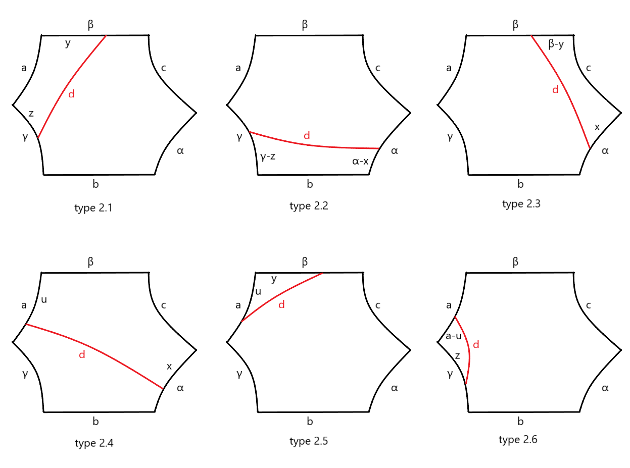
Figure 12. 6 kinds of geodesic segments in Type-2

Similar to what we do for Type-1. Denote $p,q$ and $r$ to be intersection points of $J_{j}$ and $\alpha,\beta$ and $\gamma$ respectively if they exist. Denote $x$ to be the part of $\alpha$ that from $p$ to $c$ if it exists, and $y$ to be the part of $\beta$ that from $q$ to $a$ if it exists, and $z$ to be the part of $\gamma$ that from $r$ to $a$ if it exists. We fix these points $p,q$ and $r$ as $b$ and $c$ are simultaneously decreasing, more precisely, keep the length of each $x,y$ and $z$ to be unchanged. Since $\alpha,\beta$ and $\gamma$ are increasing as $b$ and $c$ are simultaneously decreasing by Lemma 54,the points $p,q$ and $r$ will still lie in $\alpha,\beta$ and $\gamma$ respectively during the process. These intersection points separate $J_{j}$ into several segments. Fixing these points as $b$ and $c$ are simultaneously decreasing, we get a piecewise geodesic $J^{\prime\prime}_{j}$ homotopic to $J_{j}$ in $\mathcal{P}_{\delta}$.

In type 2.1, the lengths $a,y$ and $z$ are all unchanged during the process, so the corresponding $d$ is also unchanged. In types 2.5 and 2.6, the endpoints of $J_{j}$ on boundary $2a$ are fixed, so the length $u$ (part of $a$ from the endpoint of $J_{j}$ to $\beta$, see Figure 12) is also unchanged. Since $a,y$ and $z$ are all unchanged, the corresponding $d$ is also unchanged.

For the remaining $3$ kinds, similar to Type-1 we will show that

(105) $$|\dot{d}+1|=O_{A}\left(\frac{m}{b}\right)$$

and $J_{j}$ must contain at least two of those $3$ kinds.

Lemma 56.

The segment $J_{j}$ for Type-2 must contain at least two segments of types 2.2, 2.3 and 2.4 as shown in Figure 12.

Proof.

Since $\eta$ is filling, the segment $J_{j}$ is a geodesic in $\mathcal{P}$ with endpoints on $2a$ (if $X$ is not $S_{0,3}$) or just a closed geodesic in $\mathcal{P}$ (if $X$ is $S_{0,3}$). Moreover it must have at least one intersection point with $\alpha$ which is denoted by $o$. On both sides of $J_{j}$ at point $o$, there is at least one segment $d$ of type 2.2 or 2.3 or 2.4. Then the conclusion follows. ∎

Next we prove (105) for those $3$ types in Lemma 56 case by case.

Lemma 57 (types 2.2 and 2.3).

If $b\geq Am$ and (96) holds, then for types 2.2 and 2.3 in Figure 12 we have

$$|\dot{d}+1|=O_{A}\left(\frac{m}{b}\right).$$

Proof.

Recall that $\dot{x}=\dot{y}=\dot{z}=0$ and $\dot{b}=\dot{c}=-1$. For type 2.2, by Lemma 54 and we apply Lemma 43 to rectangle $(\gamma-z,b,\alpha-x,d)$ to obtain that $|\dot{d}+1|=O_{A}\left(\frac{m}{b}\right)$. For type 2.3, the proof is similar. ∎

Lemma 58 (type 2.4).

If $b\geq Am$ and (96) holds, then for type 2.4 in Figure 12 we have

$$|\dot{d}+1|=O_{A}\left(\frac{m}{b}\right).$$

Proof.

Let $h_{a}$ be the perpendicular between $a$ and $\alpha$ in type 2.4. Let $e$ to be part of $\alpha$ between $h_{a}$ and $c$, and let $f$ to be part of $a$ between $h_{a}$ and $\beta$ (see Figure 13). Then we have a rectangle $(u-f,h_{a},x-e,d)$ with $\angle(h_{a},u-f)=\angle(h_{a},x-e)=\frac{\pi}{2}$. We remark here that the lengths $u-f$ and $x-e$ may be negative. Now we compute the lengths of these edges and their derivatives.

Figure 13.

By Lemma 42 we have

(106) $$\cosh h_{a}=\sinh c\sinh\beta\ \rm{and}\ \cosh\beta=\sinh e\sinh h_{a}.$$

By (8.3) we have $\dot{\beta}=\frac{\cosh a+\cosh(b-c)}{\sinh\alpha\sinh b\sinh^{2}c}$. A direct computation shows that

$$\dot{h}_{a} = \frac{1}{\sinh h_{a}}\bigg{(}\dot{c}\cosh c\sinh\beta+\dot{\beta}\sinh c\cosh\beta\bigg{)}$$

$$= -\frac{\cosh h_{a}}{\sinh h_{a}}\frac{\cosh c}{\sinh c}+\frac{\cosh\beta}{\sinh h_{a}}\frac{(\cosh a+\cosh(b-c))}{\sinh\alpha\sinh b\sinh c}$$

$$= -\frac{\cosh h_{a}}{\sinh h_{a}}\frac{\cosh c}{\sinh c}+\frac{\sinh e}{\sinh\alpha}\frac{(\cosh a+\cosh(b-c))}{\sinh b\sinh c}.$$

Since $\sinh e\leq\sinh\alpha=\sinh w\leq 2\pi\frac{m}{b}$, we have

$$\sinh h_{a}=\frac{\cosh\beta}{\sinh e}\geq\frac{1}{2\pi}\frac{b}{m}.$$

Since $e\leq\alpha=w$, by (96) and (8.3) we have $\frac{\sinh e}{\sinh\alpha}\frac{\cosh a}{\sinh b\sinh c}\leq 2\sinh^{2}{\frac{w}{2}}\leq 8\pi^{2}\frac{m^{2}}{b^{2}}$. By Lemma 54 $\frac{\sinh e}{\sinh\alpha}\frac{\cosh\left(b-c\right)}{\sinh b\sinh c}=O_{A}\left(e^{-2b}+e^{-2c}\right)=O_{A}\left(\frac{m^{2}}{b^{2}}\right)$. Then we have

$$|\dot{h}_{a}+1| \leq \left|\frac{\cosh h_{a}}{\sinh h_{a}}\frac{\cosh c}{\sinh c}-1\right|+O_{A}\left(\frac{m^{2}}{b^{2}}\right)$$

$$= O_{A}\left(e^{-2h_{a}}+e^{-2c}+\frac{m^{2}}{b^{2}}\right)$$

$$= O_{A}\left(\frac{m^{2}}{b^{2}}\right).$$

By Lemma 42 and (106) we have

(108) $$\sinh e=\frac{\cosh\beta}{\sinh h_{a}}$$

and

(109) $$\dot{e} = \frac{1}{\cosh e}\bigg{(}\dot{\beta}\frac{\sinh\beta}{\sinh h_{a}}-\dot{h}_{a}\frac{\cosh\beta\cosh h_{a}}{\sinh^{2}h_{a}}\bigg{)}$$

$$= \frac{1}{\cosh e}\bigg{(}\dot{\beta}\frac{\cosh h_{a}}{\sinh h_{a}}\frac{1}{\sinh c}-\dot{h}_{a}\frac{\cosh h_{a}}{\sinh h_{a}}\sinh e\bigg{)}.$$

By Lemma 54, the fact that $\sinh e\leq\sinh\alpha=\sinh w\leq 2\pi\frac{m}{b}$ and the above bounds, we have $|\dot{e}|=O_{A}\left(\frac{m}{b}\right)$.

By Lemma 42 and (8.3) we have

(110) $$\sinh f=\frac{\cosh e}{\sinh\beta}$$

and

$$\quad\quad\quad\dot{f} = \frac{1}{\cosh f}\bigg{(}\dot{e}\frac{\sinh e}{\sinh\beta}-\dot{\beta}\frac{\cosh\beta\cosh e}{\sinh^{2}\beta}\bigg{)}$$

$$= \dot{e}\frac{\sinh f}{\cosh f}\frac{\sinh e}{\cosh e}-\frac{(\cosh a+\cosh(b-c))}{\sinh\alpha\sinh b\sinh^{2}c}\frac{\cosh\beta\cosh e}{\sinh e\sinh c\sinh^{2}\beta}$$

$$= \dot{e}\frac{\sinh f}{\cosh f}\frac{\sinh e}{\cosh e}-\frac{(\cosh a+\cosh(b-c))\sinh h_{a}\cosh e}{\sinh\alpha\sinh b\sinh c\cosh^{2}h_{a}}$$

$$= \dot{e}\frac{\sinh f}{\cosh f}\frac{\sinh e}{\cosh e}-\frac{\sinh e}{\sinh\alpha}\frac{\sinh^{2}h_{a}}{\cosh^{2}h_{a}}\frac{\cosh e}{\cosh\beta}\frac{(\cosh a+\cosh(b-c))}{\sinh b\sinh c}.$$

Since $\sinh e\leq 2\pi\frac{m}{b}$ and $|\dot{e}|=O_{A}\left(\frac{m}{b}\right)$, we have $\left|\dot{e}\frac{\sinh f}{\cosh f}\frac{\sinh e}{\cosh e}\right|=O_{A}\left(\frac{m^{2}}{b^{2}}\right)$. By (96) and (8.3) it is not hard to see that

$$\left|\frac{\sinh e}{\sinh\alpha}\frac{\sinh^{2}h_{a}}{\cosh^{2}h_{a}}\frac{\cosh e}{\cosh\beta}\frac{(\cosh a+\cosh(b-c))}{\sinh b\sinh c}\right| \leq \cosh e\frac{\cosh a+\cosh(b-c)}{\sinh b\sinh c}$$

$$= O_{A}\left(\frac{m^{2}}{b^{2}}\right).$$

Thus, we have $|\dot{f}|=O_{A}\left(\frac{m^{2}}{b^{2}}\right)$.

Recall that $\dot{x}=\dot{u}=0$. By Lemma 54 and all the bounds above, then we apply Lemma 43 to rectangle $(u-f,h_{a},x-e,d)$ to obtain that $|\dot{d}+1|=O_{A}\left(\frac{m}{b}\right)$. ∎

Now we are ready to prove Proposition 40 for Type-2.

Proposition 59.

Proposition 40 holds for the case that $\mathcal{P}$ is of Type-2.

Proof.

Let $2b$ to be the longest boundary geodesic of $X$, and $\mathcal{P}$ be the pants with boundary geodesics $(2a,2b,2c)$ as in the construction. Since $\sum x_{i}\geq n(2Am+\delta)$, we know $2b\geq 2Am+\delta>\frac{1}{2}\delta$. By Lemma 54, we know $\sinh c\geq\frac{b}{2\pi m}\geq\frac{A}{2\pi}$. So if $0<\delta<4\mathop{\rm arcsinh}(\frac{A}{2\pi})$, we have $2c>\frac{1}{2}\delta$. Hence both the pants $\mathcal{P}_{\delta}$ and the surface $X_{\delta}$ exist.

During the process that $b$ and $c$ reduce to $b-\frac{1}{4}\delta$ and $c-\frac{1}{4}\delta$ respectively, we denote $b^{\prime},c^{\prime},w^{\prime}$ to be the quantities corresponding to $b,c,w$ respectively. The length $a$ is unchanged. We have

$$b-\frac{1}{4}\delta\leq b^{\prime}\leq b\ \ \rm{and}\ \ c-\frac{1}{4}\delta\leq c^{\prime}\leq c.$$

So $b^{\prime}\geq Am$ always holds.

By Lemma 42 $\cosh w=\frac{\cosh a+\cosh b\cosh c}{\sinh b\sinh c}$ and then

$$\sinh^{2}w = \cosh^{2}w-1$$

$$= \frac{\cosh^{2}a+\sinh^{2}b+\sinh^{2}c+1+2\cosh a\cosh b\cosh c}{\sinh^{2}b\sinh^{2}c}.$$

So

$$\frac{\sinh w^{\prime}}{\sinh w} = \frac{\sinh b\sinh c}{\sinh b^{\prime}\sinh c^{\prime}}$$

$$\left(\frac{\cosh^{2}a+\sinh^{2}b^{\prime}+\sinh^{2}c^{\prime}+1+2\cosh a\cosh b^{\prime}\cosh c^{\prime}}{\cosh^{2}a+\sinh^{2}b+\sinh^{2}c+1+2\cosh a\cosh b\cosh c}\right)^{\frac{1}{2}}$$

$$\leq \frac{\sinh b}{\sinh(b-\frac{1}{4}\delta)}\frac{\sinh c}{\sinh(c-\frac{1}{4}\delta)}$$

$$= \left(\cosh\frac{\delta}{4}+\frac{1}{\tanh(b-\frac{\delta}{4})}\sinh\frac{\delta}{4}\right)\left(\cosh\frac{\delta}{4}+\frac{1}{\tanh(c-\frac{\delta}{4})}\sinh\frac{\delta}{4}\right)$$

$$\leq \left(\cosh\frac{\delta}{4}+\frac{\sinh\frac{\delta}{4}}{\tanh A}\right)\left(\cosh\frac{\delta}{4}+\frac{\sinh\frac{\delta}{4}}{\tanh(\mathop{\rm arcsinh}(\frac{A}{2\pi})-\frac{\delta}{4})}\right)$$

$$< 2$$

for $\delta\in(0,A_{0}]$ where $A_{0}$ is some constant only depending on $A$. Recall that (64) says that $\sinh w\leq\frac{\pi m}{b}$. So we have that for $0<\delta\leq A_{0}$, the inequality that $\sinh w^{\prime}\leq\frac{2\pi m}{b}$ always holds, i.e, equation(96) always holds. Thus the assumptions in Lemma 57 and 58 are always satisfied.

As the two boundary lengths $2b$ and $2c$ simultaneously reduce by $\frac{1}{2}\delta$, the corresponding length $d$ in types 2.1, 2.5 and 2.6 are unchanged. For remaining types 2.2, 2.3 and 2.4, it follows by Lemma 57 and 58 that the length $d$ decreases at least $\left(1-O_{A}\left(\frac{m}{b}\right)\right)\frac{\delta}{4}$. By Lemma 56 $J_{j}$ must contain at least two of the decreasing types. So we have

$$\ell(J_{j})-\ell(J^{\prime}_{j})\geq\frac{1}{2}\left(1-O_{A}\left(\frac{m}{b}\right)\right)\delta$$

which together with (66) imply that

$$\ell_{\eta}(X)-\ell_{\eta}(X_{\delta})\geq\frac{1}{2}\left(1-O_{A}\left(\frac{m}{b}\right)\right)\delta=\frac{1}{2}\left(1-O_{A}\left(\frac{mn}{\sum x_{i}}\right)\right)\delta$$

where in the last equation we apply $2b\geq\frac{\sum x_{i}}{n}$.

The proof is complete. ∎

Proof of Proposition 40.

By assumption, $\sum x_{i}\geq n(2Am+\delta)\geq 2Anm$. So we have

$$\left(\frac{mn}{\sum x_{i}}\right)^{2}\leq\frac{1}{2A}\cdot\left(\frac{mn}{\sum x_{i}}\right).$$

Then the conclusion clearly follows by Proposition 51 and 59. ∎

References

- [BBD88] Peter Buser, Marc Burger, and Jozef Dodziuk, Riemann surfaces of large genus and large , Geometry and analysis on manifolds (Katata/Kyoto, 1987), Lecture Notes in Math., vol. 1339, Springer, Berlin, 1988, pp. 54–63.
- [Ber16] Nicolas Bergeron, The spectrum of hyperbolic surfaces, Universitext, Springer, Cham; EDP Sciences, Les Ulis, 2016, Appendix C by Valentin Blomer and Farrell Brumley, Translated from the 2011 French original by Brumley [2857626].
- [BM04] Robert Brooks and Eran Makover, Random construction of Riemann surfaces, J. Differential Geom. 68 (2004), no. 1, 121–157.
- [Bus92] Peter Buser, Geometry and spectra of compact Riemann surfaces, Progress in Mathematics, vol. 106, Birkhäuser Boston, Inc., Boston, MA, 1992.
- [Che75] Shiu Yuen Cheng, Eigenvalue comparison theorems and its geometric applications, Math. Z. 143 (1975), no. 3, 289–297.
- [DGZZ20] Vincent Delecroix, Elise Goujard, Peter Zograf, and Anton Zorich, Large genus asymptotic geometry of random square-tiled surfaces and of random multicurves, arXiv e-prints (2020), arXiv:2007.04740.
- [GJ78] Stephen Gelbart and Hervé Jacquet, A relation between automorphic representations of and , Ann. Sci. École Norm. Sup. (4) 11 (1978), no. 4, 471–542.
- [GLMST21] Clifford Gilmore, Etienne Le Masson, Tuomas Sahlsten, and Joe Thomas, Short geodesic loops and norms of eigenfunctions on large genus random surfaces, Geom. Funct. Anal. 31 (2021), no. 1, 62–110.
- [GPY11] Larry Guth, Hugo Parlier, and Robert Young, Pants decompositions of random surfaces, Geom. Funct. Anal. 21 (2011), no. 5, 1069–1090.
- [Hej76] Dennis A. Hejhal, The Selberg trace formula for . Vol. I, Lecture Notes in Mathematics, Vol. 548, Springer-Verlag, Berlin-New York, 1976.
- [Hid21] Will Hide, Spectral gap for Weil-Petersson random surfaces with cusps, arXiv e-prints (2021), arXiv:2107.14555.
- [HM21] Will Hide and Michael Magee, Near optimal spectral gaps for hyperbolic surfaces, arXiv e-prints (2021), arXiv:2107.05292.
- [Hub74] Heinz Huber, Über den ersten Eigenwert des Laplace-Operators auf kompakten Riemannschen Flächen, Comment. Math. Helv. 49 (1974), 251–259.
- [Iwa89] H. Iwaniec, Selberg’s lower bound of the first eigenvalue for congruence groups, Number theory, trace formulas and discrete groups (Oslo, 1987), Academic Press, Boston, MA, 1989, pp. 371–375.
- [Iwa96] Henryk Iwaniec, The lowest eigenvalue for congruence groups, Topics in geometry, Progr. Nonlinear Differential Equations Appl., vol. 20, Birkhäuser Boston, Boston, MA, 1996, pp. 203–212.
- [Iwa02] by same author, Spectral methods of automorphic forms, second ed., Graduate Studies in Mathematics, vol. 53, American Mathematical Society, Providence, RI; Revista Matemática Iberoamericana, Madrid, 2002.
- [Jen84] Felix Jenni, Über den ersten Eigenwert des Laplace-Operators auf ausgewählten Beispielen kompakter Riemannscher Flächen, Comment. Math. Helv. 59 (1984), no. 2, 193–203.
- [Kim03] Henry H. Kim, Functoriality for the exterior square of and the symmetric fourth of , J. Amer. Math. Soc. 16 (2003), no. 1, 139–183, With appendix 1 by Dinakar Ramakrishnan and appendix 2 by Kim and Peter Sarnak.
- [KS02] Henry H. Kim and Freydoon Shahidi, Functorial products for and the symmetric cube for , Ann. of Math. (2) 155 (2002), no. 3, 837–893, With an appendix by Colin J. Bushnell and Guy Henniart.
- [Lal89] Steven P. Lalley, Renewal theorems in symbolic dynamics, with applications to geodesic flows, non-Euclidean tessellations and their fractal limits, Acta Math. 163 (1989), no. 1-2, 1–55.
- [LRS95] W. Luo, Z. Rudnick, and P. Sarnak, On Selberg’s eigenvalue conjecture, Geom. Funct. Anal. 5 (1995), no. 2, 387–401.
- [LW21] Michael Lipnowski and Alex Wright, Towards optimal spectral gaps in large genus, arXiv e-prints (2021), arXiv:2103.07496.
- [Mag20] Michael Magee, Letter to Bram Petri, https://www.maths.dur.ac.uk/users/michael.r.magee/diameter.pdf, 2020.
- [Mir07a] Maryam Mirzakhani, Simple geodesics and Weil-Petersson volumes of moduli spaces of bordered Riemann surfaces, Invent. Math. 167 (2007), no. 1, 179–222.
- [Mir07b] by same author, Weil-Petersson volumes and intersection theory on the moduli space of curves, J. Amer. Math. Soc. 20 (2007), no. 1, 1–23.
- [Mir10] by same author, On Weil-Petersson volumes and geometry of random hyperbolic surfaces, Proceedings of the International Congress of Mathematicians. Volume II, Hindustan Book Agency, New Delhi, 2010, pp. 1126–1145.
- [Mir13] by same author, Growth of Weil-Petersson volumes and random hyperbolic surfaces of large genus, J. Differential Geom. 94 (2013), no. 2, 267–300.
- [MNP20] Michael Magee, Frédéric Naud, and Doron Puder, A random cover of a compact hyperbolic surface has relative spectral gap , arXiv e-prints (2020), arXiv:2003.10911.
- [Mon15] Sugata Mondal, On largeness and multiplicity of the first eigenvalue of finite area hyperbolic surfaces, Math. Z. 281 (2015), no. 1-2, 333–348.
- [Mon20] Laura Monk, Benjamini-Schramm convergence and spectrum of random hyperbolic surfaces of high genus, Analysis & PDE (2020), to appear.
- [MP19] Maryam Mirzakhani and Bram Petri, Lengths of closed geodesics on random surfaces of large genus, Comment. Math. Helv. 94 (2019), no. 4, 869–889.
- [MZ15] Maryam Mirzakhani and Peter Zograf, Towards large genus asymptotics of intersection numbers on moduli spaces of curves, Geom. Funct. Anal. 25 (2015), no. 4, 1258–1289.
- [NWX20] Xin Nie, Yunhui Wu, and Yuhao Xue, Large genus asymptotics for lengths of separating closed geodesics on random surfaces, arXiv e-prints (2020), arXiv:2009.07538.
- [PWX21] Hugo Parlier, Yunhui Wu, and Yuhao Xue, The simple separating systole for hyperbolic surfaces of large genus, Journal of the Institute of Mathematics of Jussieu (2021), to appear.
- [Sar95] Peter Sarnak, Selberg’s eigenvalue conjecture, Notices Amer. Math. Soc. 42 (1995), no. 11, 1272–1277.
- [Sel56] A. Selberg, Harmonic analysis and discontinuous groups in weakly symmetric Riemannian spaces with applications to Dirichlet series, J. Indian Math. Soc. (N.S.) 20 (1956), 47–87.
- [Sel65] Atle Selberg, On the estimation of Fourier coefficients of modular forms, Proc. Sympos. Pure Math., Vol. VIII, Amer. Math. Soc., Providence, R.I., 1965, pp. 1–15.
- [Wol82] Scott Wolpert, The Fenchel-Nielsen deformation, Ann. of Math. (2) 115 (1982), no. 3, 501–528.
- [Wol10] Scott A. Wolpert, Families of Riemann surfaces and Weil-Petersson geometry, CBMS Regional Conference Series in Mathematics, vol. 113, Published for the Conference Board of the Mathematical Sciences, Washington, DC; by the American Mathematical Society, Providence, RI, 2010.
- [Wri20] Alex Wright, A tour through Mirzakhani’s work on moduli spaces of Riemann surfaces, Bull. Amer. Math. Soc. (N.S.) 57 (2020), no. 3, 359–408.
- [WX21] Yunhui Wu and Yuhao Xue, Small eigenvalues of closed Riemann surfaces for large genus, Transactions of the American Mathematical Society (2021), to appear.