Energy Landscape and Metastability of Stochastic Ising and Potts Models on Three-dimensional Lattices Without External Fields

Abstract.

In this study, we investigate the energy landscape of the Ising and Potts models on fixed and finite but large three-dimensional (3D) lattices where no external field exists and quantitatively characterize the metastable behavior of the associated Glauber dynamics in the very low temperature regime. Such analyses for the models with non-zero external magnetic fields have been extensively performed over the past two decades; however, models without external fields remained uninvestigated. Recently, the corresponding investigation has been conducted for the two-dimensional (2D) model without an external field, and in this study, we further extend these successes to the 3D model, which has a far more complicated energy landscape than the 2D one. In particular, we provide a detailed description of the highly complex plateau structure of saddle configurations between ground states and then analyze the typical behavior of the Glauber dynamics thereon. Thus, we acheive a quantitatively precise analysis of metastability, including the Eyring–Kramers law, the Markov chain model reduction, and a full characterization of metastable transition paths.

Example of a three-dimensional saddle configuration

1. Introduction

Metastability is a ubiquitous phenomenon that arises when a stochastic system has several locally stable sets; it is observed in a wide class of models, e.g., in the small random perturbations of dynamical systems (e.g., [15, 16, 21, 31, 33, 36, 37, 38, 46]), interacting particle systems consisting of sticky particles (e.g., [5, 11, 22, 24, 29, 30, 45, 47]), and spin systems in the low temperature regime (e.g., [1, 6, 10, 12, 13, 14, 17, 18, 20, 23, 27, 28, 32, 35, 42, 43, 40]). Numerous important works are not listed here; we direct the references of the monographs [12, 44], which provide a comprehensive introduction to this broad topic.

Metastable behaviors of stochastic Ising and Potts models

In this study, we consider the metastability of the stochastic Ising and Potts models evolving according to Metropolis–Hastings-type Glauber dynamics on a large, but fixed three-dimensional (3D) lattice. For such models, the Gibbs invariant measure is exponentially concentrated on monochromatic configurations (i.e., the configurations consisting of a single spin, which are the ground states of the Ising and Potts Hamiltonians) in the very low temperature regime. Hence, in such regimes, the dynamics exhibits metastable behavior between the monochromatic configurations: It starts from a monochromatic configuration, remains in a certain neighborhood of the starting configuration for an exponentially long time, and finally overcomes the energy barrier between monochromatic configurations to reach another monochromatic one.

Several mathematical questions persist regarding the metastable behavior explained above. For instance, in the transition from one monochromatic configuration to another, the mean transition time, the asymptotic law of the rescaled transition time, and the typical transition paths are all points of interest. We are also interested in the characterization of the energy barrier and the saddle configurations that realize this energy barrier via optimal paths between monochromatic configurations. The final issue is particularly important and challenging for the model considered in the present article and has remained open for a long time. It is also important to estimate the mixing time or spectral gap of the associated dynamics; this allows us to measure the effects of metastable behavior on the global mixing properties of the associated Markovian dynamics. In this article, we answer all these questions for the stochastic Ising and Potts models on finite three-dimensional lattices in the absence of external fields.

Model with non-zero external field

The first rigorous mathematical treatment of the metastable behavior of the Ising model was performed in [42, 43], where the authors considered the Ising model on a two-dimensional (2D) lattice in the presence of a non-zero external field. These studies verified that the transition from a metastable monochromatic configuration to a stable one is essentially equivalent to the formation of a certain type of critical droplet. From this observation, precise information regarding the transition path was obtained, as well as large deviation-type estimates for the transition time and mixing behavior associated with the Metropolis–Hastings dynamics. This result was extended to the 3D Ising model presented in [1, 6]. Similar results for four- or higher-dimensional models remain to be found, because the variational problems related to the analysis of the energy landscape and critical droplet are highly complicated.

In [17], the aforementioned analyses were further refined via the potential-theoretic approach developed in [15]. In [17], the authors obtained the Eyring–Kramers law for the transition time between monochromatic configurations, as well as the spectral gap of the associated dynamics. This new technology does not provide information on the transition path; however, it provides precise asymptotics for the mean metastable transition time and spectral gap. The same model on growing lattice boxes, rather than fixed ones, was investigated in [14], and the Kawasaki-type (instead of Glauber-type) dynamics for the same model were studied in [13].

Model without external field

When studying the metastability of the stochastic Ising model with a non-zero external field (as described above), the crucial object is the critical droplet, which provides a sharp saddle structure for the energy landscape. However, in the zero external field case, the critical droplet does not exist. Instead, the saddle structure is flat, structurally complex, and composed of a large set of saddle configurations. This is the crucial challenge in the zero external field case, which has left the problem unsolved for a long time. In the present study, we solve this problem by comprehensively analyzing the energy landscape.

Recently, [40] analyzed for the first time the 2D Ising and Potts models in the absence of external fields. More precisely, they characterized (1) the energy barrier between ground states and (2) the deepest metastable valleys in the landscape. Using the energy landscape results and a general tool referred to as the pathwise approach to metastability (developed in [18, 19, 39, 41]), they obtained large deviation-type results for the metastable behaviors of the 2D models in the absence of external fields.

In [25], which is a companion article of the present one, we improved on the refinement of results in the previous studies for the 2D model using the potential-theoretic approach, thereby making the following contributions:

• the Eyring–Kramers law for metastable transitions between monochromatic configurations,

• the Markov chain model reduction of metastable behavior (cf. [26] for a comprehensive review on this method), and

• the full characterization of typical transition paths.

To this end, we derive a highly detailed analysis of the energy landscape and characterize all saddle configurations. In particular, we comprehensively and precisely describe the large and complicated saddle structure of the model. Our analysis is sufficiently accurate to allow the transition paths between ground states to be characterized explicitly.

Main achievement

In the current article, we extend all these analyses to the 3D Ising and Potts models by combining the pathwise approach and the potential-theoretic approach. Indeed, the energy landscape of the 3D model is significantly more complicated than that of the 2D model. For both the 2D and 3D models, there are numerous saddle configurations between ground states, and they form a plateau structure. For the 2D model, at least the bulk part of this plateau structure is relatively simple, because each saddle configuration can only move forward or backward to reach another saddle configuration. In contrast, for the 3D model, we cannot expect such a simplification, because there exist certain configurations for which the legitimate movements between saddle configurations can occur in a substantially more complex manner. We refer to the figure at the front page for an example of a highly complicated saddle configuration in the 3D case (which should be characterized in some way to answer all the questions above). Readers who are familiar with the results on the non-zero external field model can notice from this figure that the saddle configurations for the zero external model may not have a clear structure as in the non-zero external field case.

Approximation method to metastability

In our companion paper [25], we introduced a new approximation method to prove the Eyring–Kramers law and Markov chain model reduction. This method relies on the approximation of the equilibrium potential function (refer to Section 3.1 for the precise definition) in a Sobolev space defined via the Dirichlet norm associated with the Markov chain. It is robust and particularly suitable if the energy landscape is too complex to apply the potential-theoretic approach [15] via variational principles (the Dirichlet and Thomson principles), because it effectively avoids these variational principles via an approximation in the Sobolev space. We apply this method to the 3D model to achieve our main result.

The main mathematical difficulty of applying this method lies in the fact that we must construct a test function that accurately approximates the equilibrium potential function so that we can obtain the precise Sobolev norm. For this procedure, we need a comprehensive understanding of the whole energy landscape regarding the metastable transitions. Thus, compared with the 2D model, the corresponding construction for the 3D model is far more complicated. Overcoming this difficulty is the main contribution of the present study.

2. Main Results

2.1. Models

In this subsection, we introduce the stochastic Ising and Potts models on a fixed 3D lattice and review their basic features.

Ising and Potts models

We fix three positive integers $K\leq L\leq M$. Then, we denote by

$$\Lambda=\llbracket 1,\,K\rrbracket\times\llbracket 1,\,L\rrbracket\times\llbracket 1,\,M\rrbracket$$

the 3D lattice box. We use the notation $\llbracket a,\,b\rrbracket=[a,\,b]\cap\mathbb{Z}$ throughout this article. We impose either open or periodic boundary conditions upon the lattice box $\Lambda$. For the latter boundary condition, we can write

$$\Lambda=\mathbb{T}_{K}\times\mathbb{T}_{L}\times\mathbb{T}_{M}\;,$$ (2.1)

where $\mathbb{T}_{k}=\mathbb{Z}/(k\mathbb{Z})$ represents the discrete one-dimensional torus.

For an integer $q\geq 2$, we use $S=\{1,\,\dots,\,q\}$ to represent the set of spins and $\mathcal{X}=S^{\Lambda}$ to represent the space of spin configurations in the 3D box $\Lambda$. We express a configuration $\sigma\in\mathcal{X}$ as $\sigma=(\sigma(x))_{x\in\Lambda}$, where $\sigma(x)\in S$ represents the spin of $\sigma$ at site $x\in\Lambda$.

For $x,\,y\in\Lambda$, we write $x\sim y$ if they are neighboring sites; that is, $\|x-y\|=1$ where $\|\cdot\|$ denotes the Euclidean distance in $\Lambda$. With this notation, we define the Hamiltonian $H:\mathcal{X}\rightarrow\mathbb{R}$ as

$$H(\sigma)=\sum_{\{x,\,y\}\subseteq\Lambda:\,x\sim y}\mathbf{1}\{\sigma(x)\neq\sigma(y)\}-h\sum_{x\in\Lambda}\sigma(x)\;\;\;\;;\;\sigma\in\mathcal{X}\;,$$ (2.2)

where $h\in\mathbb{R}$ denotes the magnitude of the external magnetic field. Thus, the first summation on the right-hand side represents the spin–spin interactions, and the second one corresponds to the effect of the external magnetic field. We use $\mu_{\beta}(\cdot)$ to denote the Gibbs measure on $\mathcal{X}$ associated with the Hamiltonian $H$ at inverse temperature $\beta>0$; that is,

$$\mu_{\beta}(\sigma)=\frac{1}{Z_{\beta}}e^{-\beta H(\sigma)}\;\;\;\;;\;\sigma\in\mathcal{X}\;,$$ (2.3)

where $Z_{\beta}=\sum_{\zeta\in\mathcal{X}}e^{-\beta H(\zeta)}$ is the partition function. The random spin configuration on box $\Lambda$ corresponds to the probability measure $\mu_{\beta}(\cdot)$ on $\mathcal{X}$; it is referred to as the Ising model if $q=2$ and the Potts model if $q\geq 3$. Henceforth, we treat $q$ as a fixed parameter. Our primary concern is the metastability analyses of these models as $\beta\rightarrow\infty$ under Metropolis–Hastings dynamics, which will be defined precisely below.

Remark 2.1 (Results for non-zero external field).

Comprehensive analyses of the energy landscape and the metastability of the Ising model with a non-zero external field i.e., $h\neq 0$, were performed in [17, 42, 43] for the 2D case, and in [1, 6] for the 3D one. For these models, the characterization of the critical droplet comprehensively explains the metastable behavior. We remark that analysis for cases of more than three dimensions has yet to be undertaken, because the energy landscape is too complex to allow critical droplets to be characterized. Recently, the 2D Potts model with an external field toward one specific spin has been studied [7, 8, 9].

In this study, we consider the zero external field case (i.e., $h=0$); thus, we henceforth assume that $h=0$. This case differs from those involving non-zero external fields, in the sense that the energy landscape is not characterized by critical droplets. Instead, we must tackle a large and complex landscape of saddle configurations via complicated combinatorial and probabilistic arguments.

Ground states

For each $a\in S$, denote by $\mathbf{s}_{a}\in\mathcal{X}$ the monochromatic configuration in which all spins are $a$, i.e., $\mathbf{s}_{a}(x)=a$ for all $x\in\Lambda$. We write

$$\mathcal{S}=\{\mathbf{s}_{1},\,\dots,\,\mathbf{s}_{q}\}\;.$$ (2.4)

It is precisely upon $\mathcal{S}$ that the Hamiltonian $H(\cdot)$ attains its minimum $0$; hence, $\mathcal{S}$ represents the set of ground states of the model. Accordingly, we obtain the following characterization of the partition function $Z_{\beta}$ that appears in (2.3), as well as the Gibbs measure $\mu_{\beta}$ as $\beta\rightarrow\infty$.

Theorem 2.2.

We have

$$Z_{\beta}=q+O_{\beta}(e^{-3\beta})\;.$$ (2.5)

Thus, we obtain

$$\lim_{\beta\rightarrow\infty}\mu_{\beta}(\mathbf{s})=\frac{1}{q}\text{ for all }\mathbf{s}\in\mathcal{S}\;\;\;\;\text{and}\;\;\;\;\lim_{\beta\rightarrow\infty}\mu_{\beta}(\mathcal{S})=1\;.$$

Proof.

The estimate (2.5) of the partition function comes directly from the expression of the partition function given right after (2.3) and the fact that $H(\sigma)\geq 3$ for $\sigma\notin\mathcal{S}$. The second assertion of the theorem is directly derived from the first one and the expression (2.3) of $\mu_{\beta}$. ∎

Metropolis–Hastings dynamics and metastability

We give a continuous version of the Metropolis–Hastings dynamics, which is the standard heat-bath Glauber dynamics used for studying the metastability of the Ising model [42]. For $x\in\Lambda$ and $a\in S$, we use $\sigma^{x,\,a}\in\mathcal{X}$ to denote the configuration obtained from $\sigma$ by updating the spin at site $x$ to $a$. Then, the continuous version of the Metropolis–Hastings dynamics is defined as a continuous-time Markov chain $\{\sigma_{\beta}(t)\}_{t\geq 0}$ on $\mathcal{X}$, whose transition rates are given by

$$r_{\beta}(\sigma,\,\zeta)=\begin{cases}e^{-\beta[H(\zeta)-H(\sigma)]_{+}}&\text{if }\zeta=\sigma^{x,\,a}\neq\sigma\text{ for some }x\in\Lambda\text{ and }a\in S\;,\\ 0&\text{otherwise}\;,\end{cases}$$

where $[\alpha]_{+}=\max\,\{\alpha,\,0\}$. We notice from this definition of the rate $r_{\beta}(\cdot,\,\cdot)$ that the Metropolis–Hastings dynamics tends to lower the energy, particularly when $\beta$ is large, because the jump rate from one configuration to another one with higher energy is exponentially small, whereas the jump rate to another one with lower or equal energy is $1$. We let $\mathbb{P}_{\sigma}^{\beta}$ and $\mathbb{E}_{\sigma}^{\beta}$ represent the law and expectation, respectively, of the process $\sigma_{\beta}(\cdot)$ starting from $\sigma$.

For $\sigma,\,\zeta\in\mathcal{X}$, we write $\sigma\sim\zeta$ if $r_{\beta}(\sigma,\,\zeta)>0$. Note that $\sigma\sim\zeta$ if and only if $\zeta\sim\sigma$, and that the relation $\sigma\sim\zeta$ does not depend on $\beta$. A crucial observation regarding the rate $r_{\beta}(\cdot,\,\cdot)$ defined above is that

$$\mu_{\beta}(\sigma)\,r_{\beta}(\sigma,\,\zeta)=\mu_{\beta}(\zeta)\,r_{\beta}(\zeta,\,\sigma)=\begin{cases}\min\,\{\mu_{\beta}(\sigma),\,\mu_{\beta}(\zeta)\}&\text{if }\sigma\sim\zeta\;,\\ 0&\text{otherwise\;.}\end{cases}$$ (2.6)

From this detailed balance condition, we observe that the invariant measure for the Metropolis–Hastings dynamics $\sigma_{\beta}(\cdot)$ is $\mu_{\beta}(\cdot)$ and that $\{\sigma_{\beta}(t)\}_{t\geq 0}$ is reversible with respect to $\mu_{\beta}(\cdot)$. We also note that the Markov chain $\sigma_{\beta}(\cdot)$ is irreducible.

In view of Theorem 2.2, we anticipate that the process $\sigma_{\beta}(\cdot)$ will exhibit metastable behavior between ground states, provided that $\beta$ is sufficiently large. More precisely, the process $\sigma_{\beta}(\cdot)$ starting from configuration $\mathbf{s}\in\mathcal{S}$ remains in a certain neighborhood of $\mathbf{s}$ for a sufficiently long time, and then undergoes a rare but rapid transition to another ground state. Our main concern is to precisely analyze such metastability of the stochastic Ising and Potts models under the Metropolis–Hastings dynamics (defined above) in the very low temperature regime; that is, when $\beta\rightarrow\infty$. We explain these results in the following subsection.

Remark 2.3.

We employ the continuous-time dynamics (as applied in numerous previous studies) because it offers a simpler presentation than the corresponding discrete dynamics (as demonstrated in [6, 17, 40]), for which the jump probability is given by

$$p_{\beta}(\sigma,\,\zeta)=\begin{cases}\frac{1}{q|\Lambda|}\,e^{-\beta[H(\zeta)-H(\sigma)]_{+}}&\text{if }\zeta=\sigma^{x,\,a}\neq\sigma\text{ for some }x\in\Lambda\;,\;a\in S\;,\\ 1-\sum_{x\in\Lambda,\,a\in S:\,\sigma^{x,a}\neq\sigma}p_{\beta}(\sigma,\,\sigma^{x,\,a})&\text{if }\zeta=\sigma\;,\\ 0&\text{otherwise}\;.\end{cases}$$ (2.7)

However, our computations can be applied to this model as well. See also Remark 2.15.

2.2. Main results: large deviation-type results

Hereafter, we explain our results regarding the metastability of the stochastic Ising and Potts models. In the current subsection, we explain the large deviation-type results obtained for the metastable behavior.

Energy barrier between ground states

First, we introduce the energy barrier associated with the Ising and Potts models considered in this study. This is important for the analysis of metastable behaviors, in that the Metropolis–Hastings dynamics must overcome this energy barrier to make a transition from one ground state to another.

A sequence of configurations $(\omega_{t})_{t=0}^{T}=(\omega_{0},\,\omega_{1},\,\dots,\,\omega_{T})\subseteq\mathcal{X}$ for some integer $T\geq 0$ is called a path if $\omega_{t}\sim\omega_{t+1}$ (i.e., $r_{\beta}(\omega_{t},\,\omega_{t+1})>0$) for all $t\in\llbracket 0,\,T-1\rrbracket$. We say that this path connects two configurations $\sigma$ and $\zeta$ if $\omega_{0}=\sigma$ and $\omega_{T}=\zeta$ or vice versa. The communication height between two configurations $\sigma,\,\zeta\in\mathcal{X}$ is defined as

$$\Phi(\sigma,\,\zeta)=\min_{(\omega_{t})_{t=0}^{T}}\,\max_{t\in\llbracket 0,\,T\rrbracket}\,H(\omega_{t})\;,$$

where the minimum is taken over all paths connecting $\sigma$ and $\zeta$. Moreover, for two disjoint subsets $\mathcal{P}$ and $\mathcal{Q}$ of $\mathcal{X}$, we define

$$\Phi(\mathcal{P},\,\mathcal{Q})=\min_{\sigma\in\mathcal{P},\,\zeta\in\mathcal{Q}}\,\Phi(\sigma,\,\zeta)\;.$$

Then, we define

$$\Gamma=\Gamma(K,\,L,\,M)=\Phi(\mathbf{s},\,\mathbf{s}^{\prime})\;\;\;\;;\;\mathbf{s},\,\mathbf{s}^{\prime}\in\mathcal{S}\;.$$

Note that $\Phi(\mathbf{s},\,\mathbf{s}^{\prime})$ does not depend on the selections of $\mathbf{s},\,\mathbf{s}^{\prime}\in\mathcal{S}$, owing to the model symmetry. Additionally, note that $\Gamma$ represents the energy barrier between ground states, because the dynamics must overcome this energy level to make a transition from one ground state to another.

To characterize the energy barrier, we must check the maximum energy of all paths connecting the ground states. Thus, the energy barrier is a global feature of the energy landscape, and characterizing it is a non-trivial task. For the current model, we can identify the exact value of the energy barrier. Recall that we assumed $K\leq L\leq M$.

Theorem 2.4.

For all sufficiently large $K$, it holds that

$$\Gamma=\begin{cases}2KL+2K+2&\text{under periodic boundary conditions}\;,\\ KL+K+1&\text{under open boundary conditions}\;.\end{cases}$$ (2.8)

Remark 2.5.

Our arguments state that this theorem holds for $K\geq 2829$, where the threshold $2829$ may be sub-optimal (cf. Remark 8.4). However, the optimality of this threshold is a minor issue, because our main concern is the spin system on large boxes. Henceforth, we assume that $K$ satisfies this condition, i.e., $K\geq 2829$.

Theorem 2.4 is proved in Section 8.

Remark 2.6.

Several remarks regarding the previous theorem are in order.

1. Note that Theorem 2.4 does not depend on the value of $q$, because in the transition from $\mathbf{s}_{a}$ to $\mathbf{s}_{b}$ for $a,\,b\in S$, no spins besides $a$ and $b$ play a significant role.

2. Suppose temporarily that $\Gamma_{d}$ is the energy barrier, defined in the same way as above, subjected to Ising/Potts models defined on a $d$-dimensional lattice box of size $K_{1}\times\cdots\times K_{d}$ with $K_{1}\leq\cdots\leq K_{d}$. Then, we expect that $\Gamma_{d}=2+2\sum_{n=1}^{d-1}\prod_{i=1}^{n}K_{i}$ under periodic boundary conditions and $\Gamma_{d}=1+\sum_{n=1}^{d-1}\prod_{i=1}^{n}K_{i}$ under open boundary conditions for all $d\geq 2$. Notice that the case of $d=2$ is handled in [40, Theorem 1.1] and the case of $d=3$ is handled in Theorem 2.4. We leave the verification of this conjecture for the case of $d\geq 4$ as a future research problem.

Comparison with non-zero external field case

We conclude this energy barrier discussion by comparing our results for the zero external field case with those for the non-zero external field case obtained in [42] and [6] for the Ising model (i.e., $q=2$) in two or three dimensions, respectively. More precisely, they showed that the energy barrier is given by (under some technical assumptions regarding $h$)

$$\Gamma_{2}(h)= \,4\ell_{h}-h[\ell_{h}(\ell_{h}-1)+1]\;,$$

$$\Gamma_{3}(h)= \,2m_{h}(2m_{h}-\delta_{h}-1)+2(m_{h}-\delta_{h})(m_{h}-1)+4\ell_{h}$$

$$\,-h[m_{h}(m_{h}-\delta_{h})(m_{h}-1)+\ell_{h}(\ell_{h}-1)+1]\;,$$

where $\Gamma_{d}$ represents the $d$-dimensional energy barrier, $\ell_{h}=\lceil 2/|h|\rceil$, $m_{h}=\lceil 4/|h|\rceil$, and $\delta_{h}\in\{0,\,1\}$ is a constant depending only on $h$ (provided that the lattice is sufficiently large). We refer to [12, Chapter 17] for details. These energy barriers are characterized by the energy of the critical droplet, and their values do not depend on the size of the box but are determined solely by the magnitude $h$ of the external field. This is primarily because the size of the critical droplet is determined solely by $|h|$, and the size of the box plays no role provided that the box is sufficiently large to contain a single droplet. In contrast, the zero external field case does not feature such a critical droplet; hence, the magnitude of the energy barrier depends crucially on the box size. This is the key difference between the zero external field and non-zero external field cases.

Large deviation-type results based on pathwise approach

Here, we explain the large deviation-type analysis of the metastable behavior of the Metropolis–Hastings dynamics. These results can be obtained via the pathwise approach developed in [18], provided that we can analyze the model energy landscape to a certain degree of precision. We refer to the monograph [44] for an extensive summary of the pathwise approach. This approach allows us to analyze the metastability from three different perspectives: transition time, spectral gap, and mixing time. All these quantities are crucial for quantifying the metastable behavior. First, we explicitly define them as follows:

• For $\mathcal{A}\subseteq\mathcal{X}$, we denote by $\tau_{\mathcal{A}}=\inf\,\{t\geq 0:\sigma_{\beta}(t)\in\mathcal{A}\}$ the hitting time of the set $\mathcal{A}$. If $\mathcal{A}=\{\sigma\}$ is a singleton, we write $\tau_{\{\sigma\}}=\tau_{\sigma}$.

• For $\mathbf{s}\in\mathcal{S}$, we write $\breve{\mathbf{s}}=\mathcal{S}\setminus\{\mathbf{s}\}$. Then, our primary concern is the hitting time $\tau_{\breve{\mathbf{s}}}$ or $\tau_{\mathbf{s}^{\prime}}$ for $\mathbf{s}^{\prime}\in\breve{\mathbf{s}}$ when the dynamics starts from $\mathbf{s}\in\mathcal{S}$. We refer to this as the (metastable) transition time, because it expresses the time required for a transition to proceed from the ground state to another one.

• The mixing time corresponding to the level $\epsilon\in(0,\,1)$ is defined as

  $$t_{\beta}^{\mathrm{mix}}(\epsilon)=\min\,\big{\{}\,t\geq 0:\max_{\sigma\in\mathcal{X}}\,\|\mathbb{P}_{\sigma}^{\beta}\,[\sigma_{\beta}(t)\in\cdot]-\mu_{\beta}(\cdot)\|_{\textrm{TV}}\leq\epsilon\,\big{\}}\;,$$

  where $\|\cdot\|_{\textrm{TV}}$ represents the total variation distance between measures (cf. [34, Chapter 4]).

• We denote by $\lambda_{\beta}$ the spectral gap of the Metropolis–Hastings dynamics defined in Section 2.1.

The 2D version of the following theorem was established in [40] using the refined pathwise approach developed in [19, 39, 41]. We extend their results to the 3D model.

Theorem 2.7.

The following statements hold.

1. (Transition time) For all $\mathbf{s},\,\mathbf{s}^{\prime}\in\mathcal{S}$ and $\epsilon>0$, we have

   $$\lim_{\beta\rightarrow\infty}\mathbb{P}_{\mathbf{s}}^{\beta}\,[e^{\beta(\Gamma-\epsilon)}<\tau_{\breve{\mathbf{s}}}\leq\tau_{\mathbf{s}^{\prime}}<e^{\beta(\Gamma+\epsilon)}]=1\;,$$ (2.9)

   $$\lim_{\beta\rightarrow\infty}\frac{1}{\beta}\log\mathbb{E}_{\mathbf{s}}^{\beta}\,[\tau_{\breve{\mathbf{s}}}]=\lim_{\beta\rightarrow\infty}\frac{1}{\beta}\log\mathbb{E}_{\mathbf{s}}^{\beta}\,[\tau_{\mathbf{s}^{\prime}}]=\Gamma\;.$$ (2.10)

   Moreover, under $\mathbb{P}_{\mathbf{s}}^{\beta}$, as $\beta\rightarrow\infty$,

   $$\frac{\tau_{\breve{\mathbf{s}}}}{\mathbb{E}_{\mathbf{s}}^{\beta}\,[\tau_{\breve{\mathbf{s}}}]}\;,\;\frac{\tau_{\mathbf{s}^{\prime}}}{\mathbb{E}_{\mathbf{s}}^{\beta}\,[\tau_{\mathbf{s}^{\prime}}]}\rightharpoonup\mathrm{Exp}(1)\;,$$ (2.11)

   where $\mathrm{Exp}(1)$ is the exponential random variable with a mean value of $1$.

2. (Mixing time) For all $\epsilon\in(0,\,1/2)$, the mixing time satisfies

   $$\lim_{\beta\rightarrow\infty}\frac{1}{\beta}\log t_{\beta}^{\mathrm{mix}}(\epsilon)=\Gamma\;.$$

3. (Spectral gap) There exist two constants $0<c_{1}\leq c_{2}$ such that

   $$c_{1}\,e^{-\beta\Gamma}\leq\lambda_{\beta}\leq c_{2}\,e^{-\beta\Gamma}\;.$$

Remark 2.8.

The above theorem holds under both open and periodic boundary conditions.

Theorem 2.7 states that the metastable transition time, mixing time, and inverse spectral gap become exponentially large as $\beta\rightarrow\infty$, and their exponential growth rates are determined by the energy barrier $\Gamma$.

The robust methodology developed in [19, 39, 41] implies that characterizing the energy barrier between ground states and identifying all the deepest valleys suffice (up to several technical issues) to confirm the results presented in Theorem 2.7. In [40], the authors performed corresponding analyses of the energy landscape; then, they used this robust methodology to prove Theorem 2.7 for two dimensions. We perform the corresponding analysis of the energy landscape for the 3D model as well in Sections 6, 7, and 8. The proof of Theorem 2.7 is given in Section 8.3. Analysis of the energy landscape is far more difficult than that of the 2D one considered in [25] for several reasons. Details are presented at the beginning of Section 6.

Characterization of transition path

Our analysis of the energy landscape is sufficiently precise to characterize all the possible transition paths between ground states in a high level of detail. The transition paths are rigorously defined in Definition 9.13; we do not present explicit definitions here, because we would have to define a large amount of notation. The following theorem asserts that, with dominating probability, the Metropolis–Hastings dynamics evolves along one of the transition paths when a transition occurs from one ground state to another.

Theorem 2.9.

For all $\mathbf{s}\in\mathcal{S}$, we have

$$\mathbb{P}_{\mathbf{s}}^{\beta}\,\big{[}\,\exists 0<t_{1}<\cdots<t_{N}<\tau_{\breve{\mathbf{s}}}\text{ such that }(\sigma_{\beta}(t_{n}))_{n=1}^{N}\text{ is a transition path between }\mathbf{s}\text{ and }\breve{\mathbf{s}}\,\big{]}$$

$$=1-o_{\beta}(1)\;.$$

The characterization of the transition paths and the proof of this theorem are given in Section 9.4.

2.3. Main results: Eyring–Kramers law and Markov chain model reduction

The following results constitute more quantitative analyses of the metastable behavior obtained using potential-theoretic methods. In particular, we obtain the Eyring–Kramers law (which is a considerable refinement of (2.10)) and the Markov chain model reduction of metastable behavior in the sense of [2, 3].

For these results, we require an accurate understanding of the energy landscape and the behavior of the Metropolis–Hastings dynamics on a large set of saddle configurations between ground states. We conduct these analyses in Sections 9 and 10.

We further remark that the quantitative results given below depend on the selection of boundary condition, in contrast to Theorems 2.7 and 2.9 (cf. Remark 2.8). For brevity, we assume periodic boundary conditions throughout this subsection. We can treat the open boundary case in a similar manner; the results and a sketch of the proof are presented in Section 11.

Eyring–Kramers law

The following result constitutes a refinement of (2.10) (and hence of (2.11)) that allows us to pin down the sub-exponential prefactor associated with the large deviation-type exponential estimates of the mean transition time between ground states.

Theorem 2.10.

There exists a constant $\kappa=\kappa(K,\,L,\,M)>0$ such that for all $\mathbf{s},\,\mathbf{s}^{\prime}\in\mathcal{S}$,

$$\mathbb{E}_{\mathbf{s}}^{\beta}\,[\tau_{\breve{\mathbf{s}}}]=(1+o_{\beta}(1))\,\frac{\kappa}{q-1}\,e^{\Gamma\beta}\;\;\;\;\text{and}\;\;\;\;\mathbb{E}_{\mathbf{s}}^{\beta}\,[\tau_{\mathbf{s}^{\prime}}]=(1+o_{\beta}(1))\,\kappa\,e^{\Gamma\beta}\;.$$ (2.12)

Moreover, the constant $\kappa$ satisfies

$$\lim_{K\rightarrow\infty}\kappa(K,\,L,\,M) =\begin{cases}1/8&\text{if }K<L<M\;,\\ 1/16&\text{if }K=L<M\text{ or }K<L=M\;,\\ 1/48&\text{if }K=L=M\;.\end{cases}$$ (2.13)

In particular, the quantity $\mathbb{E}_{\mathbf{s}}^{\beta}\,[\tau_{\breve{\mathbf{s}}}]$ represents the mean time required to jump from $\mathbf{s}$ to another ground state; hence, the first formula of (2.12) corresponds to the so-called Eyring–Kramers law for the Metropolis–Hastings dynamics.

Remark 2.11.

Here, we make several comments regarding Theorem 2.10.

1. Although we do not present the exact formula for the constant $\kappa$ in the theorem, they can be explicitly expressed in terms of potential-theoretic notions relevant to a random walk defined in a complicated space (cf. (3.10) and (3.11) for the formulas). This random walk is vague (cf. Proposition 9.9) compared with the corresponding random walk identified in [25, Proposition 6.22] for the 2D model, which reflects the complexity of the energy landscape of the 3D model compared with that of the 2D one.

2. The constant $\kappa$ is model-dependent. For different Glauber dynamics (even with identical boundary conditions), this constant may differ.

3. If $K<L<M$, the transition between ground states must occur in a specific direction; meanwhile, if $K=L<M$ or $K<L=M$, there are two possible directions for the transition. If $K=L=M$, there are six possible directions. This explains the dependence of the asymptotics of $\kappa$ on the relationships among $K$, $L$, and $M$.

The proof of Theorem 2.10 is conducted via the potential-theoretic approach, which originates from [15]. Using this approach, we can estimate the mean transition time $\mathbb{E}_{\mathbf{s}}^{\beta}\,[\tau_{\breve{\mathbf{s}}}]$ by obtaining a precise estimate of the capacity between ground states (cf. [2, Proposition 6.10]). This estimate is typically obtained from variational principles for capacities, such as the Dirichlet and Thomson principles. In contrast, we use the $H^{1}$-approximation technique developed in our companion article [25], which considerably simplifies the proof but still points out the gist of the logical structure needed to estimate the capacity.

To this end, we require precise analyses of the energy landscape and the behavior of the underlying metastable processes on a certain neighborhood of saddle configurations between metastable sets. In most other models for which the Eyring–Kramers law can be obtained via such robust strategies, the energy landscape is relatively simple; hence, the landscape only marginally presents serious mathematical issues. However, in the current model, the saddle consists of a very large collection of saddle configurations, which form a complex structure. Analyzing this structure is a highly complicated task; moreover, it is difficult to assess the behavior of the dynamics in the neighborhood of this large set with adequate precision. The achievement of these tasks is one of the main contributions of this study. We emphasize here that the $H^{1}$-approximation technique, which is used in the proof of the main results in a critical manner, is particularly handy for models with complicated landscapes, such as the one considered in this study.

Markov chain model reduction of metastable behavior

Because the transitions between ground states occur successively, analyzing all these transitions together is also an important problem in the study of metastability. The general method used is Markov chain model reduction [2, 3, 4]. In this methodology, one proves that the metastable process (accelerated by a certain scale) converges, in a suitable sense, to a Markov chain on the set of metastable sets. For our model, the target Markov chain must be a Markov chain on the collection of ground states, because each ground state corresponds to a metastable set.

To explain this result in the context of our model, we introduce trace process on ground states. In view of Theorem 2.10, we must accelerate the process by a factor $e^{\Gamma\beta}$ to observe transitions between ground states in the ordinary time scale; hence, let us denote by $\widehat{\sigma}_{\beta}(t)=\sigma_{\beta}(e^{\Gamma\beta}t)$, $t\geq 0$ the accelerated process. Then, we define a random time $T(t)$, $t\geq 0$ as

$$T(t)=\int_{0}^{t}\mathbf{1}\{\widehat{\sigma}_{\beta}(u)\in\mathcal{S}\}du\;\;\;\;;\;t\geq 0\;,$$

which measures the amount of time (up to $t$) the accelerated process spends on the ground states. Let $S(\cdot)$ be the generalized inverse of $T(\cdot)$; that is,

$$S(t)=\sup\,\{u\geq 0:T(u)\leq t\}\;\;\;\;;\;t\geq 0\;.$$

Then, the (accelerated) trace process $\{X_{\beta}(t)\}_{t\geq 0}$ on the set $\mathcal{S}$ of ground states is defined by

$$X_{\beta}(t)=\widehat{\sigma}_{\beta}(S(t))\text{ for }t\geq 0\;.$$ (2.14)

We observe that the trace process $X_{\beta}(\cdot)$ is obtained from the accelerated process $\widehat{\sigma}_{\beta}(\cdot)$ by turning off the clock whenever it is not on a ground state; thus, the process $X_{\beta}(\cdot)$ extracts information regarding the hopping dynamics on ground states. It is well known that the trace process $X_{\beta}(\cdot)$ is a continuous-time, irreducible Markov chain on $\mathcal{S}$; see [2, Proposition 6.1] for a rigorous proof.

Here, in view of the second estimate of (2.12), we define the limiting Markov chain $\{X(t)\}_{t\geq 0}$ on $\mathcal{S}$, which expresses the asymptotic behavior of the accelerated process $\widehat{\sigma}_{\beta}(\cdot)$ between the ground states as a continuous-time Markov chain with jump rate

$$r_{X}(\mathbf{s},\,\mathbf{s}^{\prime})=\kappa^{-1}\text{ for all }\mathbf{s},\,\mathbf{s}^{\prime}\in\mathcal{S}\;.$$ (2.15)

Theorem 2.12.

The following statements hold.

1. The law of the Markov chain $X_{\beta}(\cdot)$ converges to that of the limiting Markov chain $X(\cdot)$ as $\beta\rightarrow\infty$, in the usual Skorokhod topology.

2. It holds that

   $$\lim_{\beta\rightarrow\infty}\max_{\mathbf{s}\in\mathcal{S}}\,\mathbb{E}_{\mathbf{s}}^{\beta}\,\Big{[}\,\int_{0}^{t}\mathbf{1}\{\widehat{\sigma}_{\beta}(u)\notin\mathcal{S}\}du\,\Big{]}=0\;.$$

The second part of this theorem implies that the accelerated process spends a negligible amount of time in the set $\mathcal{X}\setminus\mathcal{S}$. Therefore, the trace process $X_{\beta}(\cdot)$ of $\widehat{\sigma}_{\beta}(\cdot)$ on the set $\mathcal{S}$, which is essentially obtained by neglecting the excursion of $\widehat{\sigma}_{\beta}(\cdot)$ on the set $\mathcal{X}\setminus\mathcal{S}$, is indeed a reasonable object for approximating the process $\widehat{\sigma}_{\beta}(\cdot)$. Combining this observation with the first part of the theorem implies that the limiting Markov chain $X(\cdot)$ describes the successive metastable transitions of the Metropolis–Hastings dynamics.

Remark 2.13.

The proofs of Theorems 2.10 and 2.12 are based on the potential-theoretic argument, and we present the arguments in Section 3. We conjecture that these results also hold for the cases of more than three dimensions.

Remark 2.14.

Temporarily, we denote by $E_{\mathbf{s}}$ the law of the limiting Markov chain $X(\cdot)$ starting at $\mathbf{s}\in\mathcal{S}$. Theorem 2.12 is consistent with Theorem 2.10, in that for any $\mathbf{s}^{\prime}\in\breve{\mathbf{s}}$, we have $E_{\mathbf{s}}\,[\tau_{\mathbf{s}^{\prime}}]=\kappa$.

Remark 2.15 (Discrete Metropolis–Hastings dynamics).

The only difference in the discrete dynamics defined by (2.7) is that it is $q|\Lambda|$ times slower than the continuous dynamics (in the average sense). Therefore, Theorems 2.4, 2.7, and 2.9 are valid for this dynamics without any modification. Theorems 2.10 and 2.12 hold provided that we replace the constant $\kappa$ with $\kappa^{\prime}=q|\Lambda|\,\kappa$. The rigorous verification of the result proceeds in a similar way; thus, we do not repeat it here.

Outlook of proofs of main results

To prove Theorems 2.4 and 2.7, which fall into the category of pathwise-type metastability results, we investigate the energy landscape of the Ising/Potts models on the 3D lattice $\Lambda$, as described in Sections 6, 7, and 8. Along the investigation, we present proofs of Theorems 2.4 and 2.7 in Section 8. Then, we proceed to the proofs of Theorems 2.10 and 2.12, which require more accurate analyses of the energy landscape than the previous theorems. These detailed analyses are presented in Section 9, and as a byproduct we present the proof of Theorem 2.9 in Section 9.4. Then, we present the proofs of Theorems 2.10 and 2.12 in Section 10.

Non-reversible models

The stochastic system considered in this study is the continuous-time Metropolis–Hastings spin-updating dynamics, which is reversible with respect to the Gibbs measure $\mu_{\beta}(\cdot)$. In fact, as in our companion paper [25], we can consider various dynamics with invariant measure $\mu_{\beta}(\cdot)$ but are non-reversible with respect to this measure. Since the approximation method and the pathwise approach used in the proof of the main results presented above are robust and can be used in the non-reversible setting as well, we can analyze the 3D version of the non-reversible models introduced in [25] for the 2D model and obtain similar results. However, for simplicity (as analysis of the energy landscape of the 3D model is very complicated itself), we decided not to include the non-reversible content in the current article. Readers who are interested in non-reversible generalizations can refer to [25, Sections 2.2 and 5] for details.

3. Outline of the Proof

In this section, we provide a brief summary of proof of the main results. We emphasize again that in the remainder of this article (except in Section 11), we assume periodic boundary conditions; that is, $\Lambda=\mathbb{T}_{K}\times\mathbb{T}_{L}\times\mathbb{T}_{M}$. In addition, we always assume that $K$ satisfies the condition given in Remark 2.5.

We reduce the proofs of Theorems 2.10 and 2.12 (which are the final destinations of the current article) to an estimate of the capacity between ground states (cf. Theorem 3.1), and then we reduce the proof of this capacity estimate to the construction of a certain test function (cf. Proposition 3.2) which is a proper approximation of the equilibrium potential function defined in (3.4). The construction and verification of Proposition 3.2 are done in Section 10. This procedure takes into advantage all the information on the energy landscape, analyzed in Sections 6-9.

General strategy to prove such results, which works also in non-reversible cases, was developed in our companion article [25, Section 4]. Thus, we state here only the essential ingredients in a self-contained manner and refer the interested readers to [25, Section 4] for more detail.

3.1. Capacity estimate and proof of Theorems 2.10 and 2.12

The Dirichlet form $D_{\beta}(\cdot)$ associated with the (reversible) Metropolis–Hastings dynamics $\sigma_{\beta}(\cdot)$ is given by, for $f:\mathcal{X}\rightarrow\mathbb{R}$,

$$D_{\beta}(f)=\frac{1}{2}\sum_{\sigma,\,\zeta\in\mathcal{X}}\mu_{\beta}(\sigma)\,r_{\beta}(\sigma,\,\zeta)\,\{f(\zeta)-f(\sigma)\}^{2}\;.$$ (3.1)

An alternative expression for the Dirichlet form is given as

$$D_{\beta}(f)=\langle f,\,-\mathcal{L}_{\beta}f\rangle_{\mu_{\beta}}\;,$$ (3.2)

where $\langle\cdot,\,\cdot\rangle_{\mu_{\beta}}$ is the inner product on $L^{2}(\mu_{\beta})$ and $\mathcal{L}_{\beta}$ is the generator of the original process, that is,

$$(\mathcal{L}_{\beta}f)(\sigma)=\sum_{\zeta\in\mathcal{X}}r_{\beta}(\sigma,\,\zeta)\,[f(\zeta)-f(\sigma)]\;.$$ (3.3)

For two disjoint and non-empty subsets $\mathcal{P}$ and $\mathcal{Q}$ of $\mathcal{X}$, the equilibrium potential between $\mathcal{P}$ and $\mathcal{Q}$ is the function $h_{\mathcal{P},\,\mathcal{Q}}^{\beta}:\mathcal{X}\rightarrow\mathbb{R}$ defined by

$$h_{\mathcal{P},\,\mathcal{Q}}^{\beta}(\sigma)=\mathbb{P}_{\sigma}^{\beta}\,[\tau_{\mathcal{P}}<\tau_{\mathcal{Q}}]\;.$$ (3.4)

By definition, it readily follows that $h_{\mathcal{P},\,\mathcal{Q}}^{\beta}\equiv 1\text{ on }\mathcal{P}$ and $h_{\mathcal{P},\,\mathcal{Q}}^{\beta}\equiv 0\text{ on }\mathcal{Q}$. Then, we define the capacity between $\mathcal{P}$ and $\mathcal{Q}$ as

$$\mathrm{Cap}_{\beta}(\mathcal{P},\,\mathcal{Q})=D_{\beta}(h_{\mathcal{P},\,\mathcal{Q}}^{\beta})\;.$$ (3.5)

It is well known that the equilibrium potential is the unique solution to the following equation:

$$\begin{cases}f\equiv 1&\text{on }\mathcal{P}\;,\\ f\equiv 0&\text{on }\mathcal{Q}\;,\\ \mathcal{L}_{\beta}f\equiv 0&\text{on }\mathcal{X}\setminus(\mathcal{P}\cup\mathcal{Q})\;.\end{cases}$$ (3.6)

Next, we define the constant $\kappa=\kappa(K,\,L,\,M)$ that appears in Theorems 2.10 and 2.12.

• Let $\mathfrak{m}_{K}=\lfloor K^{2/3}\rfloor$, where $\lfloor\alpha\rfloor$ is the biggest integer not bigger than $\alpha$, and let $\kappa^{\mathrm{2D}}=\kappa^{\mathrm{2D}}(K,\,L)$ be the constant that appeared in [25, (4.13)], which is defined later in (5.11) explicitly and satisfies

  $$\lim_{K\to\infty}\kappa^{\mathrm{2D}}(K,\,L)=\begin{cases}1/4&\text{if }K<L\;,\\ 1/8&\text{if }K=L\;.\end{cases}$$ (3.7)

  Then, for $n\in\llbracket 1,\,q-1\rrbracket$, the bulk constant $\mathfrak{b}(n)$ is defined explicitly as

  $$\mathfrak{b}(n)=\begin{cases}\frac{1}{n(q-n)}\cdot\frac{M-2\mathfrak{m}_{K}}{2M}\cdot\kappa^{\mathrm{2D}}(K,\,L)&\text{if }K<L<M\;,\\ \frac{1}{n(q-n)}\cdot\frac{M-2\mathfrak{m}_{K}}{2M}\cdot\kappa^{\mathrm{2D}}(K,\,L)&\text{if }K=L<M\;,\\ \frac{1}{n(q-n)}\cdot\frac{M-2\mathfrak{m}_{K}}{4M}\cdot\kappa^{\mathrm{2D}}(K,\,L)&\text{if }K<L=M\;,\\ \frac{1}{n(q-n)}\cdot\frac{M-2\mathfrak{m}_{K}}{6M}\cdot\kappa^{\mathrm{2D}}(K,\,L)&\text{if }K=L=M\;.\end{cases}$$ (3.8)

• The edge constant $\mathfrak{e}(n)$, $n\in\llbracket 1,\,q-1\rrbracket$, is defined in (9.12). Furthermore, it is verified in Proposition 9.9 that

  $$0<\mathfrak{e}(n)\leq\frac{1}{K^{1/3}}\text{ for all }n\in\llbracket 1,\,q-1\rrbracket\;.$$ (3.9)

• Then, for $n\in\llbracket 1,\,q-1\rrbracket$, we define the constant

  $$\mathfrak{c}(n)=\mathfrak{b}(n)+\mathfrak{e}(n)+\mathfrak{e}(q-n)\;.$$ (3.10)

  We remark that by definition, $\mathfrak{b}(n)=\mathfrak{b}(q-n)$ for $n\in\llbracket 1,\,q-1\rrbracket$; therefore, we have $\mathfrak{c}(n)=\mathfrak{c}(q-n)$. Finally, we define the constant $\kappa$ that appears in Theorem 2.10 as

  $$\kappa=(q-1)\mathfrak{c}(1)\;.$$ (3.11)

For $A\subseteq S$, we define (cf. (2.4))

$$\mathcal{S}(A)=\{\mathbf{s}_{a}:a\in A\}\;.$$

A pair $(A,\,B)$ of two subsets $A$ and $B$ of $S$ is referred to as a proper partition of $S$ if $A$ and $B$ are non-empty subsets of $S$ satisfying $A\cup B=S$ and $A\cap B=\emptyset$. Our aim is to estimate the capacity between $\mathcal{S}(A)$ and $\mathcal{S}(B)$ for proper partitions $(A,\,B)$ of $S$. The following theorem expresses the key capacity estimate:

Theorem 3.1.

It holds for any proper partition $(A,\,B)$ of $S$ that

$$\mathrm{Cap}_{\beta}(\mathcal{S}(A),\,\mathcal{S}(B))=\frac{1+o_{\beta}(1)}{q\mathfrak{c}(|A|)}\,e^{-\Gamma\beta}\;,$$ (3.12)

where $\mathfrak{c}(|A|)$ is the constant defined in (3.10).

We explain the strategy used to prove this theorem in Section 3.2. Here, we conclude the proofs of Theorems 2.10 and 2.12 by assuming Theorem 3.1.

Proof of Theorem 2.10.

By [2, Proposition 6.10], we have the following formula for the mean transition time:

$$\mathbb{E}_{\mathbf{s}}^{\beta}\,[\tau_{\breve{\mathbf{s}}}]=\frac{1}{\mathrm{Cap}_{\beta}(\mathbf{s},\,\breve{\mathbf{s}})}\sum_{\sigma\in\mathcal{X}}\mu_{\beta}(\sigma)\,h_{\mathbf{s},\,\breve{\mathbf{s}}}^{\beta}(\sigma)\;.$$

Using Theorem 2.2 and the fact that $h_{\mathbf{s},\,\breve{\mathbf{s}}}^{\beta}(\mathbf{s})=1$ and $h_{\mathbf{s},\,\breve{\mathbf{s}}}^{\beta}\equiv 0$ on $\breve{\mathbf{s}}$, we can rewrite the last summation as

$$\frac{1}{q}+o_{\beta}(1)+\sum_{\sigma\in\mathcal{X}\setminus\mathcal{S}}\mu_{\beta}(\sigma)\,h_{\mathbf{s},\,\breve{\mathbf{s}}}^{\beta}(\sigma)=\frac{1}{q}+o_{\beta}(1)\;,$$

where the identity follows from the trivial bound $|h_{\mathbf{s},\,\breve{\mathbf{s}}}^{\beta}|\leq 1$ (cf. (3.4)). Summing up the computations above and applying Theorem 3.1, we obtain

$$\mathbb{E}_{\mathbf{s}}^{\beta}\,[\tau_{\breve{\mathbf{s}}}]=\frac{1}{\mathrm{Cap}_{\beta}(\mathbf{s},\,\breve{\mathbf{s}})}\,\Big{[}\,\frac{1}{q}+o_{\beta}(1)\,\Big{]}=(1+o_{\beta}(1))\,\frac{\kappa}{q-1}\,e^{\Gamma\beta}\;.$$ (3.13)

We next address the second estimate of (2.12). Assume that the process $\sigma_{\beta}(\cdot)$ starts at $\mathbf{s}$ and that $\mathbf{s}\neq\mathbf{s}^{\prime}$. We define a sequence of stopping times $(J_{n})_{n=0}^{\infty}$ by $J_{0}=0$ and

$$J_{n+1}=\inf\,\{t\geq J_{n}:\sigma_{\beta}(t)\in\mathcal{S}\setminus\sigma_{\beta}(J_{n})\}\;\;\;\;;\;n\geq 0\;.$$

In other words, $(J_{n})_{n=0}^{\infty}$ is the sequence of random times at which the process $\sigma_{\beta}(\cdot)$ visits a new ground state. By (3.13) and the strong Markov property, we have for all $n\geq 0$ that

$$\mathbb{E}_{\mathbf{s}}^{\beta}\,[J_{n+1}-J_{n}]=(1+o_{\beta}(1))\,\frac{\kappa}{q-1}\,e^{\Gamma\beta}\;.$$ (3.14)

Then, we define

$$n(\mathbf{s}^{\prime})=\inf\,\{n\geq 0:\sigma_{\beta}(J_{n})=\mathbf{s}^{\prime}\}$$

such that $\tau_{\mathbf{s}^{\prime}}=J_{n(\mathbf{s}^{\prime})}$; thus, we can write

$$\tau_{\mathbf{s}^{\prime}}=\sum_{i=0}^{n(\mathbf{s}^{\prime})-1}(J_{i+1}-J_{i})\;.$$ (3.15)

Note that because we have assumed $\mathbf{s}\neq\mathbf{s}^{\prime}$, it holds that $n(\mathbf{s}^{\prime})\geq 1$. By symmetry, we observe that $n(\mathbf{s}^{\prime})$ is a geometric random variable with success probability $\frac{1}{q-1}$ that is independent of the sequence $(J_{n})_{n=0}^{\infty}$. Thus, we get from (3.14) and (3.15) that

$$\mathbb{E}_{\mathbf{s}}^{\beta}\,[\tau_{\mathbf{s}^{\prime}}]=(1+o_{\beta}(1))\,\frac{\kappa}{q-1}\,e^{\Gamma\beta}\times(q-1)=(1+o_{\beta}(1))\,\kappa\,e^{\Gamma\beta}\;.$$

Finally, from (3.7), (3.8), (3.9), and (3.10), we can easily see that $\kappa$ satisfies the asymptotics (2.13). This completes the proof. ∎

Next, we consider Theorem 2.12. The general methodology used to prove this type of Markov chain model reduction, based on potential-theoretic computations, was developed in [2, 3]. Our proof also uses the potential-theoretic approach; however, the computation is slightly simpler because the metastable sets are singletons. Before stating the proof, we remark that two alternative approaches are available for the Markov chain model reduction in the context of metastability: an approach based on the Poisson equation [31, 33, 45, 46], and one based on the resolvent equation [30, 37].

Proof of Theorem 2.12.

We first consider part (1). We denote by $r_{\beta}^{\mathrm{tr}}:\mathcal{S}\times\mathcal{S}\rightarrow[0,\,\infty)$ the transition rate of the trace process $X_{\beta}(\cdot)$. In view of the rate (2.15) of the limiting Markov chain, it suffices to prove that $r_{\beta}^{\mathrm{tr}}(\mathbf{s},\,\mathbf{s}^{\prime})=(1+o_{\beta}(1))\,\frac{1}{\kappa}$ for all $\mathbf{s},\,\mathbf{s}^{\prime}\in\mathcal{S}$. Since $r_{\beta}(\mathbf{s},\,\mathbf{s}^{\prime})$ does not depend on the selections of $\mathbf{s},\,\mathbf{s}^{\prime}\in\mathcal{S}$ by the symmetry of the model, it remains to prove that

$$r_{\beta}^{\mathrm{tr}}(\mathbf{s},\,\breve{\mathbf{s}})=(1+o_{\beta}(1))\,\frac{q-1}{\kappa}\;\;\;\;\text{for all }\mathbf{s}\in\mathcal{S}\;.$$ (3.16)

We denote by $\mathbf{E}_{\mathbf{s}}^{\beta}$ the law of the trace process $X_{\beta}(\cdot)$ starting at $\mathbf{s}$. Then,

$$\frac{1}{r_{\beta}^{\mathrm{tr}}(\mathbf{s},\,\breve{\mathbf{s}})}=\mathbf{E}_{\mathbf{s}}^{\beta}\,[\tau_{\breve{\mathbf{s}}}]=e^{-\Gamma\beta}\,\mathbb{E}_{\mathbf{s}}^{\beta}\,\Big{[}\,\int_{0}^{\tau_{\breve{\mathbf{s}}}}\mathbf{1}\{\sigma_{\beta}(t)\in\mathcal{S}\}dt\,\Big{]}\;,$$ (3.17)

where the factor $e^{-\Gamma\beta}$ is included because we accelerated the process by the factor $e^{\Gamma\beta}$ when defining the trace process; the integrand $\mathbf{1}\{\sigma_{\beta}(t)\in\mathcal{S}\}$ arises because the trace process is obtained from the accelerated process by turning off the clock when the process resides outside $\mathcal{S}$. Then, by [2, Proposition 6.10], we can write

$$\mathbb{E}_{\mathbf{s}}^{\beta}\,\Big{[}\,\int_{0}^{\tau_{\breve{\mathbf{s}}}}\mathbf{1}\{\sigma_{\beta}(t)\in\mathcal{S}\}dt\,\Big{]}=\frac{1}{\mathrm{Cap}_{\beta}(\mathbf{s},\,\breve{\mathbf{s}})}\sum_{\sigma\in\mathcal{X}}\mu_{\beta}(\sigma)\,\mathbf{1}\{\sigma\in\mathcal{S}\}\,h_{\mathbf{s},\,\breve{\mathbf{s}}}^{\beta}(\sigma)=\frac{\mu_{\beta}(\mathbf{s})}{\mathrm{Cap}_{\beta}(\mathbf{s},\,\breve{\mathbf{s}})}\;,$$

where the second identity follows from the fact that $h_{\mathbf{s},\,\breve{\mathbf{s}}}^{\beta}(\mathbf{s})=1$ and $h_{\mathbf{s},\,\breve{\mathbf{s}}}^{\beta}\equiv 0$ on $\breve{\mathbf{s}}$. Therefore, by Theorems 2.2 and 3.1, we obtain

$$\mathbb{E}_{\mathbf{s}}^{\beta}\,\Big{[}\,\int_{0}^{\tau_{\breve{\mathbf{s}}}}\mathbf{1}\{\sigma_{\beta}(t)\in\mathcal{S}\}dt\,\Big{]}=(1+o_{\beta}(1))\,\frac{\kappa}{q-1}\,e^{\Gamma\beta}\;.$$

Inserting this into (3.17) yields (3.16).

Here, we address part (2). Denote by $\mathbb{P}_{\mu_{\beta}}^{\beta}$ the law of the Metropolis–Hastings dynamics $\sigma_{\beta}(\cdot)$ for which the initial distribution is $\mu_{\beta}$. Then, for any $u>0$, we obtain

$$\mathbb{P}_{\mathbf{s}}^{\beta}\,[\sigma_{\beta}(u)\notin\mathcal{S}]\leq\frac{1}{\mu_{\beta}(\mathbf{s})}\,\mathbb{P}_{\mu_{\beta}}^{\beta}\,[\sigma_{\beta}(u)\notin\mathcal{S}]=\frac{\mu_{\beta}(\mathcal{X}\setminus\mathcal{S})}{\mu_{\beta}(\mathbf{s})}\;,$$ (3.18)

where the final identity holds because $\mu_{\beta}$ is the invariant distribution. Therefore by the Fubini theorem,

$$\mathbb{E}_{\mathbf{s}}^{\beta}\,\Big{[}\,\int_{0}^{t}\mathbf{1}\{\widehat{\sigma}_{\beta}(u)\notin\mathcal{S}\}du\,\Big{]}=\int_{0}^{t}\mathbb{P}_{\mathbf{s}}^{\beta}\,[\sigma_{\beta}(e^{\Gamma\beta}u)\notin\mathcal{S}]du\leq t\cdot\frac{\mu_{\beta}(\mathcal{X}\setminus\mathcal{S})}{\mu_{\beta}(\mathbf{s})}\;,$$

which vanishes as $\beta\rightarrow\infty$ by Theorem 2.2. ∎

3.2. $H^{1}$-approximation of equilibrium potential and proof of Theorem 3.1

We fix a proper partition $(A,\,B)$ of $S$, and explain the general strategy to prove Theorem 3.1, that is, to estimate the capacity $\mathrm{Cap}_{\beta}(\mathcal{S}(A),\,\mathcal{S}(B))$.

The methodology explained here is based on [25, Section 4.5], in which it is demonstrated that finding a suitable $H^{1}$-approximation of the equilibrium potential $h_{\mathcal{S}(A),\,\mathcal{S}(B)}^{\beta}$ between $\mathcal{S}(A)$ and $\mathcal{S}(B)$ is sufficient to establish the capacity estimate. The following proposition states this result.

Proposition 3.2 ($H^{1}$-approximation of the equilibrium potential).

For any proper partition $(A,\,B)$ of $S$, there exists a function $\widetilde{h}=\widetilde{h}_{\mathcal{S}(A),\,\mathcal{S}(B)}^{\beta}:\mathcal{X}\rightarrow\mathbb{R}$ such that the following properties hold.

1. The function $\widetilde{h}$ approximates $h_{\mathcal{S}(A),\,\mathcal{S}(B)}^{\beta}$ in the sense that

   $$D_{\beta}(h_{\mathcal{S}(A),\,\mathcal{S}(B)}^{\beta}-\widetilde{h})=o_{\beta}(e^{-\beta\Gamma})\;.$$ (3.19)

2. It holds that

   $$D_{\beta}(\widetilde{h})=\frac{1+o_{\beta}(1)}{q\mathfrak{c}(|A|)}\,e^{-\Gamma\beta}\;.$$ (3.20)

Remark 3.3.

The following statements are remarks on the previous proposition.

1. Since the (square root of the) Dirichlet form can be regarded as an $H^{1}$-seminorm, by (3.19), the test function $\widetilde{h}$ approximates $h_{\mathcal{S}(A),\,\mathcal{S}(B)}^{\beta}$ in the $H^{1}$-sense.

2. Property (3.20) is the one that should be satisfied by the equilibrium potential, provided that Theorem 3.1 holds in view of (3.5).

3. Proposition 3.2 has a simpler form compared to the original one [25, Proposition 4.4], because here we only need to consider the case when $(A,\,B)$ is a proper partition of $S$.

4. Finding the test function $\widetilde{h}$ requires precise information on the energy landscape and a deep insight into typical patterns of the Metropolis–Hastings dynamics in a suitable neighborhood of saddle configurations. We derive this in Sections 6-9. Then, the construction of the test function $\widetilde{h}$ and the proof of Proposition 3.2 are given in Section 10.

Finally, provided that Proposition 3.2 holds, we prove Theorem 3.1.

Proof of Theorem 3.1.

By the triangle inequality for the seminorm $D_{\beta}(\cdot)^{1/2}$, it holds that

$$D_{\beta}(\widetilde{h})^{1/2}-D_{\beta}(h_{\mathcal{S}(A),\,\mathcal{S}(B)}^{\beta}-\widetilde{h})^{1/2}\leq D_{\beta}(h_{\mathcal{S}(A),\,\mathcal{S}(B)}^{\beta})^{1/2}\leq D_{\beta}(\widetilde{h})^{1/2}+D_{\beta}(h_{\mathcal{S}(A),\,\mathcal{S}(B)}^{\beta}-\widetilde{h})^{1/2}\;.$$

Hence, by (3.19) and (3.20), we obtain

$$D_{\beta}(h_{\mathcal{S}(A),\,\mathcal{S}(B)}^{\beta})=\frac{1+o_{\beta}(1)}{q\mathfrak{c}(|A|)}\,e^{-\Gamma\beta}\;.$$

By (3.5), the last display completes the proof. ∎

Hence, to prove the main results given in Theorems 2.10 and 2.12, it remains to prove Proposition 3.2. The proof is given in Section 10.

4. Neighborhood of Configurations

In this section, we introduce several notions of neighborhoods of configurations, which are analogues of the same concepts defined in [25, Section 6.1]. These notions will be crucially used in the characterization of energy landscape and in the construction of test objects.

For $c\in\mathbb{R}$, a path $(\omega_{t})_{t=0}^{T}$ in $\mathcal{X}$ is called a $c$-path if it is a path in the sense of Section 2.2, and moreover satisfies $H(\omega_{t})\leq c$ for all $t\in\llbracket 0,\,T\rrbracket$. Moreover, we say that this path is in $\mathcal{P}\subseteq\mathcal{X}$ if $\omega_{t}\in\mathcal{P}$ for all $t\in\llbracket 0,\,T\rrbracket$.

Definition 4.1 (Neighborhood of configurations).

1. For $\sigma\in\mathcal{X}$, the neighborhood $\mathcal{N}(\sigma)$ and the extended neighborhood $\widehat{\mathcal{N}}(\sigma)$ are defined as

   $$\mathcal{N}(\sigma) =\{\zeta\in\mathcal{X}:\text{There exists a }(\Gamma-1)\text{-path }(\omega_{t})_{t=0}^{T}\text{ connecting }\sigma\text{ and }\zeta\}\;\text{and}$$

   $$\widehat{\mathcal{N}}(\sigma) =\{\zeta\in\mathcal{X}:\text{There exists a }\Gamma\text{-path }(\omega_{t})_{t=0}^{T}\text{ connecting }\sigma\text{ and }\zeta\}\;.$$

   We set $\mathcal{N}(\sigma)=\emptyset$ (resp. $\widehat{\mathcal{N}}(\sigma)=\emptyset$) if $H(\sigma)>\Gamma-1$ (resp. $H(\sigma)>\Gamma$). Then for $\mathcal{P}\subseteq\mathcal{X}$, we define

   $$\mathcal{N}(\mathcal{P})=\bigcup_{\sigma\in\mathcal{P}}\mathcal{N}(\sigma)\;\;\;\;\text{and}\;\;\;\;\widehat{\mathcal{N}}(\mathcal{P})=\bigcup_{\sigma\in\mathcal{P}}\mathcal{\widehat{\mathcal{N}}}(\sigma)\;.$$

2. Let $\mathcal{Q}\subseteq\mathcal{X}$. For $\sigma\in\mathcal{X}$ such that $\sigma\notin\mathcal{Q}$, we define

   $$\widehat{\mathcal{N}}(\sigma\,;\,\mathcal{Q})=\{\zeta\in\mathcal{X}:\text{There exists a }\Gamma\text{-path in }\mathcal{X}\setminus\mathcal{Q}\text{ connecting }\sigma\text{ and }\zeta\}\;.$$

   As before, we set $\widehat{\mathcal{N}}(\sigma\,;\,\mathcal{Q})=\emptyset$ if $H(\sigma)>\Gamma$. Then for $\mathcal{P}\subseteq\mathcal{X}$ disjoint with $\mathcal{Q}$, define

   $$\widehat{\mathcal{N}}(\mathcal{P}\,;\,\mathcal{Q})=\bigcup_{\sigma\in\mathcal{P}}\widehat{\mathcal{N}}(\sigma\,;\,\mathcal{Q})\;.$$

With this notation, by the definition of $\Gamma$, it holds that $\mathcal{N}(\mathbf{s})\cap\mathcal{N}(\mathbf{s}^{\prime})=\emptyset$ and $\widehat{\mathcal{N}}(\mathbf{s})=\widehat{\mathcal{N}}(\mathbf{s}^{\prime})$ for any $\mathbf{s},\,\mathbf{s}^{\prime}\in\mathcal{S}$. Moreover, in the spirit of the large deviation principle, the only configurations relevant to the study of metastability are the ones in $\widehat{\mathcal{N}}(\mathcal{S})$. Hence, it is crucial to understand the structure of the set $\widehat{\mathcal{N}}(\mathcal{S})$. That is the content of Proposition 9.6.

We conclude this section with an elementary lemma which will be used in several instances of our discussion. The proof is well explained in [25, Lemma A.1], and thus we omit the detail.

Lemma 4.2.

Suppose that $\mathcal{P}$ and $\mathcal{Q}$ are disjoint subsets of $\mathcal{X}$. Then, it holds that

$$\widehat{\mathcal{N}}(\mathcal{P}\cup\mathcal{Q})=\widehat{\mathcal{N}}(\mathcal{Q}\,;\,\mathcal{P})\cup\widehat{\mathcal{N}}(\mathcal{P}\,;\,\mathcal{Q})\;.$$

5. Review of Two-dimensional Model

In this section, we recall some crucial 2D results on the energy landscape from [25, Sections 6, 7 and Appendices B, C], which are needed in our investigation of the 3D model. Since all the results that appear in the current section are proved in [25], we refer to the proofs therein.

Notation.

Greek letters $\eta$ and $\xi$ are used to denote the spin configurations of the 2D model, while letters $\sigma$ and $\zeta$ are used to denote the 3D configurations. We use the superscript $\mathrm{2D}$ to stress the notation for the 2D model; for example, we shall denote by $H^{\mathrm{2D}}(\cdot)$ the Hamiltonian of the 2D model to distinguish with $H(\cdot)$ which denotes the Hamiltonian of the 3D model.

5.1. 2D stochastic Ising and Potts models with periodic boundary conditions

We denote by $\Lambda^{\mathrm{2D}}=\mathbb{T}_{K}\times\mathbb{T}_{L}$ the 2D lattice with periodic boundary conditions. Recall that $S=\{1,\,2,\,\dots,\,q\}$ denotes the set of spins, and denote by $\mathcal{X}^{\mathrm{2D}}=S^{\Lambda^{\mathrm{2D}}}$ the space of spin configurations on the 2D lattice. Then, the 2D Ising/Potts Hamiltonian function $H^{\mathrm{2D}}:\mathcal{X}^{\mathrm{2D}}\rightarrow\mathbb{R}$ (without external field) is defined by

$$H^{\mathrm{2D}}(\eta)=\sum_{\{x,\,y\}\subseteq\Lambda^{\mathrm{2D}}:\,x\sim y}\mathbf{1}\{\eta(x)\neq\eta(y)\}\;\;\;\;;\;\eta\in\mathcal{X}^{\mathrm{2D}}\;.$$ (5.1)

We denote by $\mathbf{s}_{a}^{\mathrm{2D}}$, $a\in S$ the 2D monochromatic configurations of spin $a$, that is, $\mathbf{s}_{a}^{\mathrm{2D}}(x)=a$ for all $x\in\Lambda^{\mathrm{2D}}$. Then, it is straightforward that the ground states of this Hamiltonian is also the monochromatic configurations, i.e., the collection $\mathcal{S}^{\mathrm{2D}}$ of the ground states is given as

$$\mathcal{S}^{\mathrm{2D}}=\{\mathbf{s}_{1}^{\mathrm{2D}},\,\mathbf{s}_{2}^{\mathrm{2D}},\,\dots,\,\mathbf{s}_{q}^{\mathrm{2D}}\}\;.$$

Then, we write $\mu_{\beta}^{\mathrm{2D}}(\cdot)$ the associated 2D Gibbs measure, i.e.,

$$\mu_{\beta}^{\mathrm{2D}}(\eta)=\frac{1}{Z_{\beta}^{\mathrm{2D}}}e^{-\beta H^{\mathrm{2D}}(\eta)}\;\;\;\;;\;\eta\in\mathcal{X}^{\mathrm{2D}}\;.$$

Here, $Z_{\beta}^{\mathrm{2D}}$ is the 2D partition function with the property that (cf. [25, Theorem 2.1])

$$\lim_{\beta\to\infty}Z_{\beta}^{\mathrm{2D}}=q\;.$$ (5.2)

In the 2D model, we also consider the continuous-time Metropolis–Hastings dynamics whose transition rate is defined as

$$r_{\beta}^{\mathrm{2D}}(\eta,\,\xi)=\begin{cases}e^{-\beta[H^{\mathrm{2D}}(\xi)-H^{\mathrm{2D}}(\eta)]_{+}}&\text{if }\xi=\eta^{x,\,a}\neq\eta\text{ for some }x\in\Lambda^{\mathrm{2D}}\text{ and }a\in S\;,\\ 0&\text{otherwise}\;.\end{cases}$$

This 2D stochastic Ising/Potts model is thoroughly analyzed in our companion article [25]. The remainder of this section presents a review of our analysis.

5.2. Energy barrier and canonical transition paths

It is verified in [40, Theorem 2.1] that the energy barrier between the ground states of the 2D model is given by

$$\Gamma^{\mathrm{2D}}=2K+2\;.$$

Then, by replacing $\Gamma$ that appears in Definition 4.1 with $\Gamma^{\mathrm{2D}}$, we get two types of neighborhoods $\mathcal{N}^{\mathrm{2D}}$ and $\widehat{\mathcal{N}}^{\mathrm{2D}}$ for the 2D model. In this subsection, we explain a class of natural optimal transition paths that achieve this energy level. These paths are denoted as canonical paths. To define these paths, we first define the so-called canonical configurations. We note that the constructions given here is a brief survey of [25, Section 6.2].

Canonical configurations

The following notation is used throughout the article (also for the 3D model).

Notation 5.1.

Suppose that $N\geq 2$ is a positive integer.

• Define $\mathfrak{S}_{N}$ as the collection of connected subsets of $\mathbb{T}_{N}$. For example, if $N=6$, few examples of the elements of $\mathfrak{S}_{6}$ are $\emptyset$, $\{2,\,3\}$, $\{5,\,6,\,1\}$, $\{4,\,5,\,6,\,1,\,2\}$, $\mathbb{T}_{6}$, etc.

• For $P,\,P^{\prime}\in\mathfrak{S}_{N}$, we write $P\prec P^{\prime}$ if $P\subseteq P^{\prime}$ and $|P^{\prime}|=|P|+1$.

• A sequence $(P_{m})_{m=0}^{N}$ of sets in $\mathfrak{S}_{N}$ is called an increasing sequence if it satisfies

  $$\emptyset=P_{0}\prec P_{1}\prec\cdots\prec P_{N}=\mathbb{T}_{N}$$

  so that $|P_{m}|=m$ for all $m\in\llbracket 0,\,N\rrbracket$.

We first introduce the pre-canonical configurations which are illustrated in Figure 5.1.

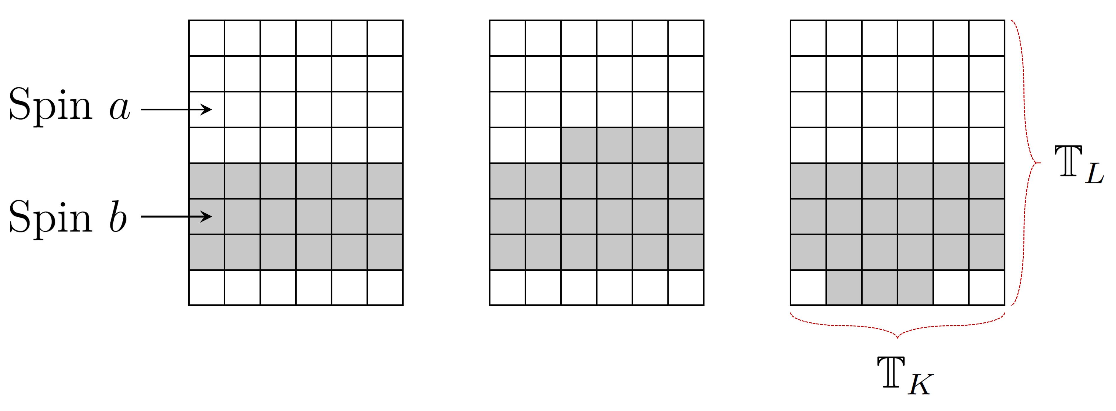
Figure 5.1. 2D pre-canonical configurations. These configurations illustrate $\xi_{2,\,3}^{a,\,b}$, $\xi_{2,\,3;\,3,\,4}^{a,\,b,\,+}$, and $\xi_{2,\,3;\,2,\,3}^{a,\,b,\,-}$, respectively.

Definition 5.2 (2D pre-canonical configurations).

Fix two spins $a,\,b\in S$.

• For $\ell\in\mathbb{T}_{L}$ and $v\in\llbracket 0,\,L\rrbracket$, we denote by $\xi_{\ell,\,v}^{a,\,b}\in\mathcal{X}^{\mathrm{2D}}$ the configuration whose spins are $b$ on

  $$\mathbb{T}_{K}\times\{\ell+n\in\mathbb{T}_{L}:n\in\llbracket 0,\,v-1\rrbracket\subseteq\mathbb{Z}\}\;.$$

  and $a$ on the remainder.

• For $\ell\in\mathbb{T}_{L}$, $v\in\llbracket 0,\,L-1\rrbracket$, $k\in\mathbb{T}_{K}$, and $h\in\llbracket 0,\,K\rrbracket$, we denote by $\xi_{\ell,\,v;\,k,\,h}^{a,\,b,\,+}\in\mathcal{X}^{\mathrm{2D}}$ the configuration whose spins are $b$ on

  $$\big{\{}\,x\in\Lambda^{\mathrm{2D}}:\xi_{\ell,\,v}^{a,\,b}(x)=b\,\big{\}}\cup\big{[}\,\{k+n\in\mathbb{T}_{K}:n\in\llbracket 0,\,h-1\rrbracket\subseteq\mathbb{Z}\}\times\{\ell+v\}\,\big{]}$$

  and $a$ on the remainder. Similarly, $\xi_{\ell,\,v;\,k,\,h}^{a,\,b,\,-}\in\mathcal{X}^{\mathrm{2D}}$ is the configuration whose spins are $b$ on

  $$\big{\{}\,x\in\Lambda^{\mathrm{2D}}:\xi_{\ell,\,v}^{a,\,b}(x)=b\,\big{\}}\cup\big{[}\,\{k+n\in\mathbb{T}_{K}:n\in\llbracket 0,\,h-1\rrbracket\subseteq\mathbb{Z}\}\times\{\ell-1\}\,\big{]}$$

  and $a$ on the remainder. The configurations defined here are 2D pre-canonical configurations.

Based on this definition, the 2D canonical and regular configurations are defined.

Definition 5.3 (2D canonical and regular configurations).

Fix $a,\,b\in S$. The definitions are slightly different for the case of $K<L$ and the case of $K=L$.

• (Case $K<L$) Collection $\mathcal{C}^{a,\,b,\,\mathrm{2D}}$ of 2D canonical configurations between $\mathbf{s}_{a}^{\mathrm{2D}}$ and $\mathbf{s}_{b}^{\mathrm{2D}}$ is defined by

  $$\mathcal{C}^{a,\,b,\,\mathrm{2D}}=\bigcup_{\ell\in\mathbb{T}_{L}}\bigcup_{v\in\llbracket 0,\,L\rrbracket}\{\xi_{\ell,\,v}^{a,\,b}\}\cup\bigcup_{\ell\in\mathbb{T}_{L}}\bigcup_{v\in\llbracket 0,\,L-1\rrbracket}\bigcup_{k\in\mathbb{T}_{K}}\bigcup_{h\in\llbracket 1,\,K-1\rrbracket}\{\xi_{\ell,\,v;\,k,\,h}^{a,\,b,\,+},\,\xi_{\ell,\,v;\,k,\,h}^{a,\,b,\,-}\}\;.$$

  Then, the collection of canonical configurations is given as

  $$\mathcal{C}^{\mathrm{2D}}=\bigcup_{a,\,b\in S}\mathcal{C}^{a,\,b,\,\mathrm{2D}}\;.$$ (5.3)

  Similarly,

  $$\mathcal{R}_{v}^{a,\,b,\,\mathrm{2D}}=\bigcup_{\ell\in\mathbb{T}_{L}}\{\xi_{\ell,\,v}^{a,\,b}\}\;\;\;\;\text{and}\;\;\;\;\mathcal{Q}_{v}^{a,\,b,\,\mathrm{2D}}=\bigcup_{\ell\in\mathbb{T}_{L}}\bigcup_{k\in\mathbb{T}_{K}}\bigcup_{h\in\llbracket 1,\,K-1\rrbracket}\{\xi_{\ell,\,v;\,k,\,h}^{a,\,b,\,\pm}\}\;,$$

  and then define $\mathcal{R}_{v}^{\mathrm{2D}}=\bigcup_{a,\,b\in S}\mathcal{R}_{v}^{a,\,b,\,\mathrm{2D}}$ and $\mathcal{Q}_{v}^{\mathrm{2D}}=\bigcup_{a,\,b\in S}\mathcal{Q}_{v}^{a,\,b,\,\mathrm{2D}}$. A configuration in $\mathcal{R}_{v}^{\mathrm{2D}}$ is called a 2D regular configuration.

• (Case $K=L$) Define an operator $\Theta:\mathcal{X}^{\mathrm{2D}}\rightarrow\mathcal{X}^{\mathrm{2D}}$ as a transpose operator, i.e.,

  $$(\Theta(\sigma))(k,\,\ell)=\sigma(\ell,\,k)\;\;\;\;;\;k\in\mathbb{T}_{K}\text{ and }\ell\in\mathbb{T}_{L}\;.$$ (5.4)

  Denote temporarily by $\widetilde{\mathcal{C}}^{a,\,b,\,\mathrm{2D}}$ the collection $\mathcal{C}^{a,\,b,\,\mathrm{2D}}$ defined in the case of $K<L$ above. Then for $a,\,b\in S$, we define the collections of 2D canonical configurations between $\mathbf{s}_{a}^{\mathrm{2D}}$ and $\mathbf{s}_{b}^{\mathrm{2D}}$ as

  $$\mathcal{C}^{a,\,b,\,\mathrm{2D}}=\widetilde{\mathcal{C}}^{a,\,b,\,\mathrm{2D}}\cup\Theta(\widetilde{\mathcal{C}}^{a,\,b,\,\mathrm{2D}})\;\;\;\;\text{and}\;\;\;\;\mathcal{C}^{\mathrm{2D}}=\bigcup_{a,\,b\in S}\mathcal{C}^{a,\,b,\,\mathrm{2D}}\;.$$

  Similarly, we may define the collections $\mathcal{R}_{v}^{a,\,b,\,\mathrm{2D}}$, $\mathcal{R}_{v}^{\mathrm{2D}}$, $\mathcal{Q}_{v}^{a,\,b,\,\mathrm{2D}}$, and $\mathcal{Q}_{v}^{\mathrm{2D}}$.

Canonical paths

Now, we explain natural optimal paths between monochromatic configurations (illustrated in Figure 5.2) that consist of canonical configurations.

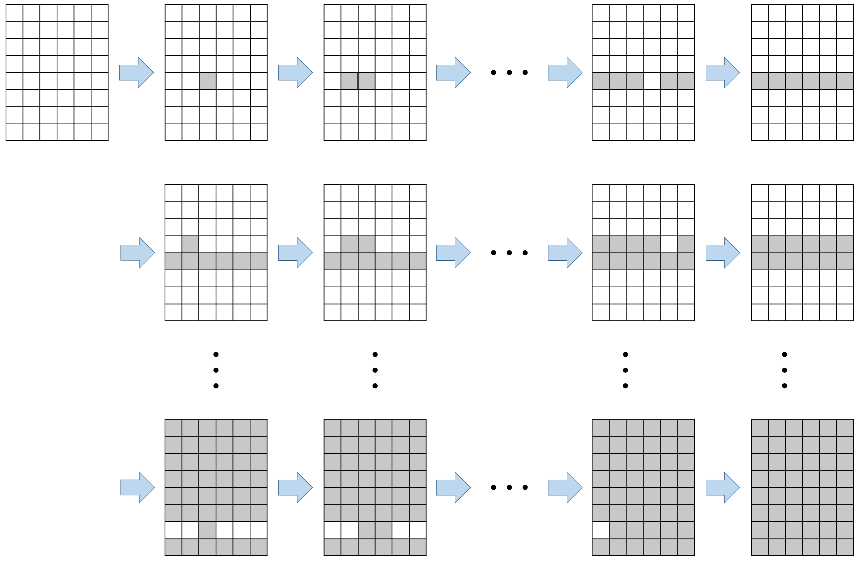
Figure 5.2. Example of a 2D canonical path from $\mathbf{s}_{a}^{\mathrm{2D}}$ to $\mathbf{s}_{b}^{\mathrm{2D}}$.

Definition 5.4 (2D canonical paths).

The definition below relies on Notation 5.1.

1. For $P,\,P^{\prime}\in\mathfrak{S}_{L}$ with $P\prec P^{\prime}$, a sequence $(A_{k})_{k=0}^{K}$ of subsets of $\Lambda^{\mathrm{2D}}$ is a standard sequence connecting $\mathbb{T}_{K}\times P$ and $\mathbb{T}_{K}\times P^{\prime}$ if there exists an increasing sequence $(Q_{k})_{k=0}^{K}$ in $\mathfrak{S}_{K}$ such that

   $$A_{k}=(\mathbb{T}_{K}\times P)\cup\big{[}\,Q_{k}\times(P^{\prime}\setminus P)\,\big{]}\;\;\;\;;\;k\in\llbracket 0,\,K\rrbracket\;.$$

2. A sequence $(A_{n})_{n=0}^{KL}$ of subsets of $\Lambda^{\mathrm{2D}}$ is a standard sequence connecting $\emptyset$ and $\Lambda^{\mathrm{2D}}$ if there exists an increasing sequence $(P_{\ell})_{\ell=0}^{L}$ in $\mathfrak{S}_{L}$ such that $A_{K\ell}=\mathbb{T}_{K}\times P_{\ell}$ for all $\ell\in\llbracket 0,\,L\rrbracket$, and furthermore for each $\ell\in\llbracket 0,\,L-1\rrbracket$ the subsequence $(A_{k})_{k=K\ell}^{K(\ell+1)}$ is a standard sequence connecting $\mathbb{T}_{K}\times P_{\ell}$ and $\mathbb{T}_{K}\times P_{\ell+1}$.

3. For $a,\,b\in S$, a sequence $(\omega_{n})_{n=0}^{KL}$ of 2D configurations is called a pre-canonical path from $\mathbf{s}_{a}^{\mathrm{2D}}$ to $\mathbf{s}_{b}^{\mathrm{2D}}$ if there exists a standard sequence $(A_{n})_{n=0}^{KL}$ connecting $\emptyset$ and $\Lambda^{\mathrm{2D}}$ such that

   $$\omega_{n}(x)=\begin{cases}a&\text{if }x\notin A_{n}\;,\\ b&\text{if }x\in A_{n}\;.\end{cases}$$

4. Moreover, a sequence $(\omega_{n})_{n=0}^{KL}$ of 2D configurations is called a canonical path (cf. Figure 5.2) connecting $\mathbf{s}_{a}^{\mathrm{2D}}$ and $\mathbf{s}_{b}^{\mathrm{2D}}$ if there exists a pre-canonical path $(\widetilde{\omega}_{n})_{n=0}^{KL}$ such that

   1. (Case $K<L$) $\omega_{n}=\widetilde{\omega}_{n}$ for all $n\in\llbracket 0,\,KL\rrbracket$,

   2. (Case $K=L$) $\omega_{n}=\widetilde{\omega}_{n}$ for all $n\in\llbracket 0,\,KL\rrbracket$ or $\omega_{n}=\Theta(\widetilde{\omega}_{n})$ for all $n\in\llbracket 0,\,KL\rrbracket$.

It holds that $H^{\mathrm{2D}}(\eta)\leq 2K+2$ for all $\eta\in\mathcal{C}^{a,\,b,\,\mathrm{2D}}$ and

$$H^{\mathrm{2D}}(\eta)=\begin{cases}2K&\text{if }\eta\in\mathcal{R}_{v}^{a,\,b,\,\mathrm{2D}}\text{ for }v\in\llbracket 1,\,L-1\rrbracket\;,\\ 2K+2&\text{if }\eta\in\mathcal{Q}_{v}^{a,\,b,\,\mathrm{2D}}\text{ for }v\in\llbracket 1,\,L-2\rrbracket\;.\end{cases}$$ (5.5)

Moreover, the following lemma is immediate.

Lemma 5.5 ([25, Lemma 6.12]).

For a 2D canonical path $(\omega_{n})_{n=0}^{KL}$ connecting $\mathbf{s}_{a}^{\mathrm{2D}}$ and $\mathbf{s}_{b}^{\mathrm{2D}}$, it holds that

$$\max_{n\in\llbracket 0,\,KL\rrbracket}H^{\mathrm{2D}}(\omega_{n})=\Gamma^{\mathrm{2D}}=2K+2\;.$$

Comment on depth of valleys

We conclude this subsection with an application of Definition 5.4 and Lemma 5.5 that is crucially used later to calculate the 3D valley depths.

Lemma 5.6 ([25, Lemma B.4]).

Let $\eta\in\mathcal{X}^{\mathrm{2D}}$ and $a\in S$. For any standard sequence $(A_{k})_{k=0}^{KL}$ of sets connecting $\emptyset$ and $\Lambda^{\mathrm{2D}}$ and for $n\in\llbracket 0,\,KL\rrbracket$, we define $\omega_{n}\in\mathcal{X}^{\mathrm{2D}}$ as

$$\omega_{n}(x)=\begin{cases}a&\text{if }x\in A_{n}\;,\\ \eta(x)&\text{if }x\in\Lambda^{\mathrm{2D}}\setminus A_{n}\;.\end{cases}$$

Then, we have that $H^{\mathrm{2D}}(\omega_{n})\leq H^{\mathrm{2D}}(\eta)+\Gamma^{\mathrm{2D}}$ for all $n\in\llbracket 0,\,KL\rrbracket$.

In Lemma 5.6, we have $\omega_{KL}=\mathbf{s}_{a}^{\mathrm{2D}}\in\mathcal{S}^{\mathrm{2D}}$ which implies that every $\eta\in\mathcal{X}^{\mathrm{2D}}$ is connected to each ground state in $\mathcal{S}^{\mathrm{2D}}$ with maximum energy $H^{\mathrm{2D}}(\eta)+\Gamma^{\mathrm{2D}}$. This fact implies that the maximum depth of valleys in the 2D energy landscape is $\Gamma^{\mathrm{2D}}$.

It can be further proved that only the valleys containing the ground states have maximum depth $\Gamma^{\mathrm{2D}}$, and all the other valleys have depth strictly less than $\Gamma^{\mathrm{2D}}$. Indeed, this is a necessary condition for the pathwise approach technique to metastability; however, this level of precision is not necessarily needed in our investigation of the 3D energy landscape. Thus, we do not go further into this direction and refer the interested readers to [40, Theorem 2.1-(ii)].

5.3. Saddle structure

Crucial configurations in the description of the saddle structure of the 2D model is the so-called typical configurations, which turn out to be the elements of the extended neighborhood $\widehat{\mathcal{N}}^{\mathrm{2D}}(\mathcal{S}^{\mathrm{2D}})$ (cf. Proposition 5.8 below). We present in Figure 5.3 an illustration of the saddle structure explained in this subsection.

Figure 5.3. Saddle structure of the 2D Ising model with $S=\{1,\,2\}$. For simplicity, we drop the superscripts $\mathrm{2D}$ in this figure.

Definition 5.7 (2D typical configurations).

There are two different types of typical configurations: the bulk and edge typical configurations.

• For $a,\,b\in S$, the collection of bulk typical configurations (between $\mathbf{s}_{a}^{\mathrm{2D}}$ and $\mathbf{s}_{b}^{\mathrm{2D}}$) is defined by

  $$\mathcal{B}^{a,\,b,\,\mathrm{2D}}=\bigcup_{v\in\llbracket 2,\,L-2\rrbracket}\mathcal{R}_{v}^{a,\,b,\,\mathrm{2D}}\cup\bigcup_{v\in\llbracket 2,\,L-3\rrbracket}\mathcal{Q}_{v}^{a,\,b,\,\mathrm{2D}}\;.$$ (5.6)

  Then, we write $\mathcal{B}^{\mathrm{2D}}=\bigcup_{a,\,b\in S}\mathcal{B}^{a,\,b,\,\mathrm{2D}}$.

• Next, define

  $$\mathcal{B}_{\Gamma}^{a,\,b,\,\mathrm{2D}}=\bigcup_{v\in\llbracket 2,\,L-3\rrbracket}\mathcal{Q}_{v}^{a,\,b,\,\mathrm{2D}}\;\;\;\;\text{and}\;\;\;\;\mathcal{B}_{\Gamma}^{\mathrm{2D}}=\bigcup_{a,\,b\in S}\mathcal{B}_{\Gamma}^{a,\,b,\,\mathrm{2D}}=\bigcup_{a,\,b\in S}\bigcup_{v\in\llbracket 2,\,L-3\rrbracket}\mathcal{Q}_{v}^{a,\,b,\,\mathrm{2D}}\;.$$ (5.7)

  Then, for $a\in S$, the collection of edge typical configurations with respect to $\mathbf{s}_{a}^{\mathrm{2D}}$ is defined by

  $$\mathcal{E}^{a,\,\mathrm{2D}}=\widehat{\mathcal{N}}^{\mathrm{2D}}(\mathbf{s}_{a}^{\mathrm{2D}}\,;\,\mathcal{B}_{\Gamma}^{\mathrm{2D}})\;.$$ (5.8)

  Finally, we write $\mathcal{E}^{\mathrm{2D}}=\bigcup_{a\in S}\mathcal{E}^{a,\,\mathrm{2D}}$.

Then, the following crucial proposition provides the picture of the saddle structure of the 2D model. We shall provide a similar result for the 3D model in Proposition 9.6.

Proposition 5.8 ([25, Proposition 6.16]).

1. For spins $a,\,b,\,c\in S$, we have

   $$\mathcal{E}^{a,\,\mathrm{2D}}\cap\mathcal{E}^{b,\,\mathrm{2D}}=\emptyset\;,\;\;\;\mathcal{E}^{a,\,\mathrm{2D}}\cap\mathcal{B}^{a,\,b,\,\mathrm{2D}}=\mathcal{R}_{2}^{a,\,b,\,\mathrm{2D}}\;\;\;\text{and}\;\;\;\mathcal{E}^{a,\,\mathrm{2D}}\cap\mathcal{B}^{b,\,c,\,\mathrm{2D}}=\emptyset\;.$$

2. It holds that $\mathcal{E}^{\mathrm{2D}}\cup\mathcal{B}^{\mathrm{2D}}=\widehat{\mathcal{N}}^{\mathrm{2D}}(\mathcal{S}^{\mathrm{2D}})$.

Gateway configurations

Next, we introduce the gateway configurations.

Definition 5.9 (2D gateway configurations).

Fix $a,\,b\in S$. Define

$$\mathcal{Z}^{a,\,b,\,\mathrm{2D}}:=\{\eta\in\mathcal{X}^{\mathrm{2D}}: \;\text{There exists a path }(\omega_{t})_{t=0}^{T}\text{ in }\mathcal{X}^{\mathrm{2D}}\setminus\mathcal{B}_{\Gamma}^{\mathrm{2D}}\text{ with }T\geq 1\text{ such that }$$

$$\;\omega_{0}\in\mathcal{R}_{2}^{a,\,b,\,\mathrm{2D}}\;,\;\omega_{T}=\eta\text{ and }H^{\mathrm{2D}}(\omega_{t})=\Gamma^{\mathrm{2D}}\text{ for all }t\in\llbracket 1,\,T\rrbracket\}\;.$$ (5.9)

Intuitively, this set is the collection of saddle configurations between $\mathcal{R}_{2}^{a,\,b,\,\mathrm{2D}}$ and $\mathbf{s}_{a}^{\mathrm{2D}}$. Then, we recall the 2D gateway configurations [25, Section B.5]. The gateway between $\mathbf{s}_{a}^{\mathrm{2D}}$ and $\mathbf{s}_{b}^{\mathrm{2D}}$ is denoted as

$$\mathcal{G}^{a,\,b,\,\mathrm{2D}}=\mathcal{Z}^{a,\,b,\,\mathrm{2D}}\cup\mathcal{B}^{a,\,b,\,\mathrm{2D}}\cup\mathcal{Z}^{b,\,a,\,\mathrm{2D}}\;,$$ (5.10)

which is a decomposition of $\mathcal{G}^{a,\,b,\,\mathrm{2D}}$. A configuration belonging to $\mathcal{G}^{a,\,b,\,\mathrm{2D}}$ is called a gateway configuration between $\mathbf{s}_{a}^{\mathrm{2D}}$ and $\mathbf{s}_{b}^{\mathrm{2D}}$.

Here, $\mathcal{G}^{a,\,b,\,\mathrm{2D}}$ is named the collection of gateway configurations because of the following lemma, which indicates that it indeed contains the saddle configurations between $\mathbf{s}_{a}^{\mathrm{2D}}$ and $\mathbf{s}_{b}^{\mathrm{2D}}$.

Lemma 5.10 ([25, Lemma B.10]).

For $a,\,b\in S$, suppose that two 2D configurations $\eta$ and $\xi$ satisfy

$$\eta\in\mathcal{G}^{a,\,b,\,\mathrm{2D}}\;,\;\xi\notin\mathcal{G}^{a,\,b,\,\mathrm{2D}}\;,\;\eta\sim\xi\;,\;\text{and}\;H^{\mathrm{2D}}(\xi)\leq\Gamma^{\mathrm{2D}}\;.$$

Then, we have either $\xi\in\mathcal{N}^{\mathrm{2D}}(\mathbf{s}_{a}^{\mathrm{2D}})$ and $\eta\in\mathcal{Z}^{a,\,b,\,\mathrm{2D}}$ or $\xi\in\mathcal{N}^{\mathrm{2D}}(\mathbf{s}_{b}^{\mathrm{2D}})$ and $\eta\in\mathcal{Z}^{b,\,a,\,\mathrm{2D}}$. In particular, $\eta\notin\mathcal{B}^{a,\,b,\,\mathrm{2D}}$.

We note that the construction of regular, canonical, typical, and gateway configurations, as well as canonical paths for the 2D model, will be extended to the 3D model in the remainder of the article.

5.4. Test function

We also recall the 2D test function defined in [25, Section 7]. Although the construction therein was carried out for both Ising and Potts models, we only need the objects for the Ising model in this article. Hence, in this subsection, we assume that $q=2$.

Recall that we always assume $K\leq L$. We recall a constant

$$\kappa^{\mathrm{2D}}=\kappa^{\mathrm{2D}}(K,\,L)$$ (5.11)

from [25, (4.13)], which plays the role of $\kappa$ in the current article and also satisfies

$$\lim_{K\to\infty}\kappa^{\mathrm{2D}}(K,\,L)=\begin{cases}1/4&\text{if }K<L\;,\\ 1/8&\text{if }K=L\;.\end{cases}$$ (5.12)

In [25, Definition 7.2], a test function $\widetilde{h}^{\mathrm{2D}}:\mathcal{X}^{\mathrm{2D}}\rightarrow\mathbb{R}$ (corresponding to $\widetilde{h}$ of the 3D model introduced in Proposition 3.2) is constructed as an $H^{1}$-approximation of the equilibrium potential between two ground states. We proclaim that this function is crucially used in the construction of the 3D test function $\widetilde{h}$. In the proof of Proposition 3.2, some estimates of $\widetilde{h}^{\mathrm{2D}}$ are crucially used. The next estimate is used in the proof of (3.20).

Proposition 5.11 ([25, Proposition C.1]).

There exists a function $\widetilde{h}^{\mathrm{2D}}:\mathcal{X}^{\mathrm{2D}}\rightarrow\mathbb{R}$ such that

$$\sum_{\{\eta,\,\xi\}\subseteq\mathcal{X}^{\mathrm{2D}}:\,\{\eta,\,\xi\}\cap\mathcal{G}^{1,\,2,\,\mathrm{2D}}\neq\emptyset}\mu_{\beta}^{\mathrm{2D}}(\eta)\,r_{\beta}^{\mathrm{2D}}(\eta,\,\xi)\,\{\widetilde{h}^{\mathrm{2D}}(\xi)-\widetilde{h}^{\mathrm{2D}}(\eta)\}^{2} =\frac{1+o_{\beta}(1)}{2\kappa^{\mathrm{2D}}}\,e^{-\Gamma^{\mathrm{2D}}\beta}\;.$$

The next one is crucially used in the proof of (3.19).

Proposition 5.12 ([25, Lemmas 7.10-7.16]).

1. For all $\eta\in\mathcal{X}^{\mathrm{2D}}\setminus\mathcal{N}^{\mathrm{2D}}(\mathcal{S}^{\mathrm{2D}})$, it holds that

   $$\sum_{\xi\in\mathcal{X}^{\mathrm{2D}}}\mu_{\beta}^{\mathrm{2D}}(\eta)\,r_{\beta}^{\mathrm{2D}}(\eta,\,\xi)\,[\widetilde{h}^{\mathrm{2D}}(\eta)-\widetilde{h}^{\mathrm{2D}}(\xi)]=o_{\beta}(e^{-\Gamma^{\mathrm{2D}}\beta})\;.$$

2. We have that

   $$\sum_{\eta\in\mathcal{N}^{\mathrm{2D}}(\mathbf{s}_{1}^{\mathrm{2D}})}\,\sum_{\xi\in\mathcal{X}^{\mathrm{2D}}}\mu_{\beta}^{\mathrm{2D}}(\eta)\,r_{\beta}^{\mathrm{2D}}(\eta,\,\xi)\,[\widetilde{h}^{\mathrm{2D}}(\eta)-\widetilde{h}^{\mathrm{2D}}(\xi)] =(1+o_{\beta}(1))\times\frac{1}{2\kappa^{\mathrm{2D}}}\,e^{-\Gamma^{\mathrm{2D}}\beta}\;,$$

   $$\sum_{\eta\in\mathcal{N}^{\mathrm{2D}}(\mathbf{s}_{2}^{\mathrm{2D}})}\,\sum_{\xi\in\mathcal{X}^{\mathrm{2D}}}\mu_{\beta}^{\mathrm{2D}}(\eta)\,r_{\beta}^{\mathrm{2D}}(\eta,\,\xi)\,[\widetilde{h}^{\mathrm{2D}}(\eta)-\widetilde{h}^{\mathrm{2D}}(\xi)] =-(1+o_{\beta}(1))\times\frac{1}{2\kappa^{\mathrm{2D}}}\,e^{-\Gamma^{\mathrm{2D}}\beta}\;.$$

5.5. Auxiliary results

In this subsection, we summarize two auxiliary results of the 2D model that are crucially used in our arguments.

Bridges, crosses and a bound on 2D Hamiltonian

For a configuration $\eta\in\mathcal{X}^{\mathrm{2D}}$, a bridge, which is a horizontal or vertical bridge, is a row or column, respectively, in which all spins are the same. If a bridge consists of spin $a\in S$, we call this bridge an $a$-bridge. Then, we denote by $B_{a}(\eta)$ the number of $a$-bridges with respect to $\eta$. A cross (resp. $a$-cross) is the union of a horizontal bridge and a vertical bridge (resp. $a$-bridges). With this notation, we have the following lower bound.

Lemma 5.13 ([25, Lemma B.2]).

It holds that

$$H^{\mathrm{2D}}(\eta)\geq 2\Big{[}\,K+L-\sum_{a\in S}B_{a}(\eta)\,\Big{]}\;.$$

Characterization of configurations with low energy

Let $a\in S$. For $\eta\in\mathcal{X}^{\mathrm{2D}}$ and $\sigma\in\mathcal{X}$ (a 3D configuration), we write

$$\|\eta\|_{a}=\sum_{x\in\Lambda^{\mathrm{2D}}}\mathbf{1}\{\eta(x)=a\}\;\;\;\;\text{and}\;\;\;\;\|\sigma\|_{a}=\sum_{x\in\Lambda}\mathbf{1}\{\sigma(x)=a\}\;.$$ (5.13)

The following proposition characterizes all the 2D configurations with energy less than $\Gamma^{\mathrm{2D}}$.

Proposition 5.14 ([25, Proposition B.3]).

Suppose that $\eta\in\mathcal{X}^{\mathrm{2D}}$ satisfies $H^{\mathrm{2D}}(\eta)<\Gamma^{\mathrm{2D}}$. Then, $\eta$ satisfies exactly one of the following properties.

• (L1) There exist $a,\,b\in S$ and $v\in\llbracket 2,\,L-2\rrbracket$ such that $\eta\in\mathcal{R}_{v}^{a,\,b,\,\mathrm{2D}}$. Here, $\mathcal{N}^{\mathrm{2D}}(\eta)=\{\eta\}$.

• (L2) There exist $a,\,b\in S$ such that $\eta\in\mathcal{R}_{1}^{a,\,b,\,\mathrm{2D}}$. In this case, $\mathcal{N}^{\mathrm{2D}}(\eta)=\mathcal{N}^{\mathrm{2D}}(\mathbf{s}_{a}^{\mathrm{2D}})$.

• (L3) For some $a\in S$, $\eta$ has an $a$-cross. Then, $\mathcal{N}^{\mathrm{2D}}(\eta)=\mathcal{N}^{\mathrm{2D}}(\mathbf{s}_{a}^{\mathrm{2D}})$ and

  $$\sum_{b\neq a}\|\eta\|_{b}\leq\frac{H^{\mathrm{2D}}(\eta)^{2}}{16}\leq\frac{(2K+1)^{2}}{16}\;.$$ (5.14)

6. Canonical Configurations and Paths

Analyzing the energy landscape of the 3D model is far more complex than that of the 2D model; below, we briefly list the main differences between them that serve to complexify the problem.

1. In the 2D model, the energy of the gateway configuration is either $\Gamma^{\mathrm{2D}}$ or $\Gamma^{\mathrm{2D}}-2$. Thus, a $\Gamma^{\mathrm{2D}}$-path on the gateway configurations does not have the freedom to move. On the other hand, in the 3D model, the energy of the gateway configuration ranges from $\Gamma-2K-2$ to $\Gamma$. This implies that the behavior of a $\Gamma$-path around a gateway configuration of energy $\Gamma-2K-2$ (which is a regular configuration) cannot be characterized precisely.

2. In the 2D model, a $\Gamma^{\mathrm{2D}}$-path from $\mathbf{s}_{a}^{\mathrm{2D}}$ to $\mathbf{s}_{b}^{\mathrm{2D}}$ must visit a configuration in $\mathcal{R}_{2}^{a,\,b,\,\mathrm{2D}}$. Then, it successively visits $\mathcal{R}_{3}^{a,\,b,\,\mathrm{2D}}$, …, $\mathcal{R}_{L-2}^{a,\,b,\,\mathrm{2D}}$ and finally arrives at $\mathbf{s}_{b}^{\mathrm{2D}}$. Remarkably, this path does not need to visit a configuration in $\mathcal{R}_{1}^{a,\,b,\,\mathrm{2D}}$ and in $\mathcal{R}_{L-1}^{a,\,b,\,\mathrm{2D}}$; this fact essentially arises from the features of the 2D geometry. In the 3D model, we observe a similar phenomenon. To explain this, let us temporarily denote by $\mathcal{R}_{v}^{a,\,b}$, $v\in\llbracket 1,\,L-1\rrbracket$ the collection of 3D configurations such that there are $v$ consecutive $K\times L$ slabs of spins $b$ and such that the spins at the remaining sites are $a$. Then, there exists an integer $n=n_{K,\,L,\,M}$ such that any $\Gamma$-path connecting $\mathbf{s}_{a}$ and $\mathbf{s}_{b}$ must successively visit configurations in $\mathcal{R}_{n}^{a,\,b}$, $\mathcal{R}_{n+1}^{a,\,b}$, $\dots,$ $\mathcal{R}_{M-n}^{a,\,b}$ but need not visit $\mathcal{R}_{i}^{a,\,b}$ for $i\in\llbracket 1,\,n-1\rrbracket$ and $i\in\llbracket M-n+1,\,M-1\rrbracket$. In the 2D model, the number corresponding to this $n=n_{K,\,L,\,M}$ is $2$. We guess that in the 3D model, $n\sim K^{1/2}$; however, we cannot determine the exact value of $n$. This fact reveals the complex structure of the energy landscape in the 3D model. Instead, we prove below (cf. Propositions 6.14 and 8.1) that

   $$\lfloor K^{1/2}\rfloor\leq n\leq\lfloor K^{2/3}\rfloor\;.$$

   Fortunately, this bound suffices to complete our analysis without identifying the exact value of $n$.

3. In the 2D model, the $\mathcal{N}^{\mathrm{2D}}$-neighborhoods are fully characterized in Proposition 5.14; meanwhile, in the 3D case, we cannot obtain such a specific and simple result. We overcome the absence of this result by using the 2D result obtained in Proposition 5.14, through suitably applying it to the analysis of the 3D model. Indeed, this absence is a crucial difficulty in extending the analysis to the four- or higher-dimensional models.

4. Because of the aforementioned complexity of the energy landscape, the transition may encounter a dead-end with energy $\Gamma$, even in the bulk part of the transition; this is not the case in the 2D model. Therefore, another technical challenge is that of carefully characterizing these dead-ends and appropriately excluding them from the computation.

As explained above, the energy landscape of the 3D model is more complex than that of the 2D one, and we are unable to present a complete description of the energy landscape for the former. Nevertheless, we analyze the landscape with the precision required to prove our main results.

In Section 6, we introduce canonical configurations and paths. Their definitions are direct generalizations of those in the 2D model. Then, we explain several applications of these canonical objects.

We first collect several notation which will be frequently used throughout the remainder of the article.

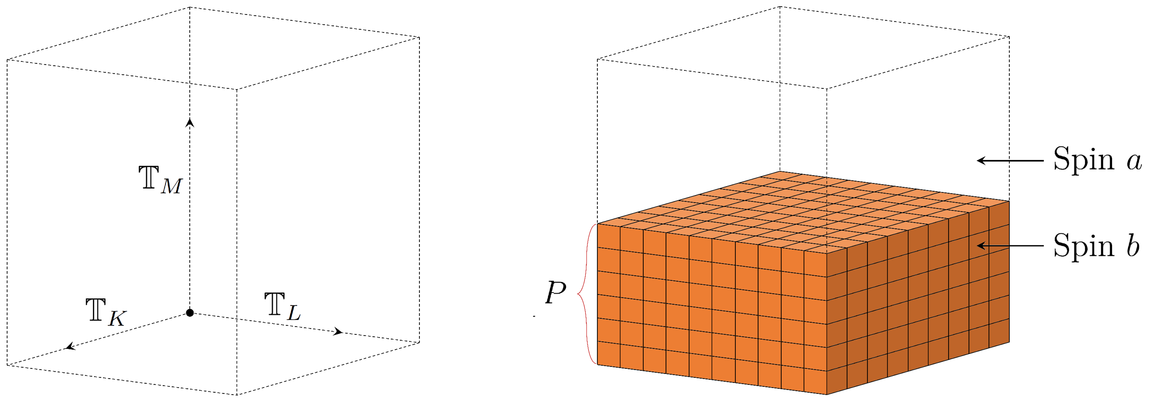
Figure 6.1. Figures on Notation 6.1. This form of figure is used throughout the remainder of the article to illustrate a 3D configuration consisting of two types of spins only. The large dotted box denotes $\Lambda=\mathbb{T}_{K}\times\mathbb{T}_{L}\times\mathbb{T}_{M}$. The orange unit boxes denote the sites with spin $b$, and the empty part denotes the cluster of spin $a$. For some cases when we only concern the shape of the cluster of spin $b$ (e.g. in Figure 6.2), we omit the dotted box representing $\Lambda$.

Notation 6.1.

We refer to Figure 6.1 for an illustration of the notation below.

• For $m\in\mathbb{T}_{M}$, the slab $\mathbb{T}_{K}\times\mathbb{T}_{L}\times\{m\}\subseteq\Lambda$ is called an $m$-th floor. For each configuration $\sigma\in\mathcal{X}$, we denote by $\sigma^{(m)}$ the configuration of $\sigma$ at the $m$-th floor, i.e.,

  $$\sigma^{(m)}(k,\,\ell)=\sigma(k,\,\ell,\,m)\;\;\;\;;\;k\in\mathbb{T}_{K}\;,\;\ell\in\mathbb{T}_{L}\;.$$ (6.1)

  Thus, $\sigma^{(m)}\in\mathcal{X}^{\mathrm{2D}}$ is a spin configuration in $\Lambda^{\mathrm{2D}}=\mathbb{T}_{K}\times\mathbb{T}_{L}.$

• For $a,\,b\in S$ and $P\subseteq\mathbb{T}_{M}$, we denote by $\sigma_{P}^{a,\,b}\in\mathcal{X}$ the configuration satisfying

  $$\sigma_{P}^{a,\,b}(k,\,\ell,\,m)=b\cdot\mathbf{1}\{m\in P\}+a\cdot\mathbf{1}\{m\notin P\}\;.$$ (6.2)

6.1. Canonical configurations

The following notation is used frequently.

Notation 6.2.

We first introduce several maps on $\mathcal{X}$. If $K=L$, we define a bijection $\Theta^{(12)}:\mathcal{X}\rightarrow\mathcal{X}$ as the map switching the first and second coordinates, i.e., for all $\sigma\in\mathcal{X}$ and $(k,\,\ell,\,m)\in\Lambda$,

$$(\Theta^{(12)}(\sigma))(k,\,\ell,\,m)=\sigma(\ell,\,k,\,m)\;.$$

If $L=M$, we can similarly define a bijection $\Theta^{(23)}$ on $\mathcal{X}$ switching the second and third coordinates. Finally, for the case of $K=L=M$, we can even define the bijection $\Theta^{(13)}$ on $\mathcal{X}$ switching the first and third coordinates.

Then, for $\mathcal{A}\subseteq\mathcal{X}$, we define $\Upsilon(\mathcal{A})$ as

$$\Upsilon(\mathcal{A})=\begin{cases}\mathcal{A}&\text{if }K<L<M\;,\\ \mathcal{A}\cup\Theta^{(12)}(\mathcal{A})&\text{if }K=L<M\;,\\ \mathcal{A}\cup\Theta^{(23)}(\mathcal{A})&\text{if }K<L=M\;,\\ \begin{aligned} &\mathcal{A}\cup\Theta^{(12)}(\mathcal{A})\cup\Theta^{(23)}(\mathcal{A})\cup\Theta^{(13)}(\mathcal{A})\\ &\cup(\Theta^{(12)}\circ\Theta^{(23)})(\mathcal{A})\cup(\Theta^{(23)}\circ\Theta^{(12)})(\mathcal{A})\end{aligned}&\text{if }K=L=M\;.\end{cases}$$

Note that the set $\Upsilon(\mathcal{A})$ for the case of $K=L=M$ denotes the set of all configurations obtained by permuting the coordinates of the configurations in $\mathcal{A}$.

Now, we define canonical configurations of our 3D model.

Figure 6.2. Canonical configurations. These two configurations belong to $\mathcal{C}_{6}^{a,\,b}$ (if the orange boxes represent the sites with spin $b$ as in Figure 6.1), since the 2D configurations at the $7$-th floor are 2D canonical configurations $\xi_{6,\,7;\,5,\,2}^{a,\,b,\,+}$ and $\xi_{3,\,4;\,2,\,6}^{a,\,b,\,-}$, respectively.

Definition 6.3 (Canonical configurations).

We refer to Figure 6.2 for a visualization of the objects introduced below. Recall Notation 5.1.

1. We first introduce some building blocks in the definition of canonical and gateway configurations. For $a,\,b\in S$ and $P,\,Q\in\mathfrak{S}_{M}$ with $P\prec Q$, we define $\widetilde{\mathcal{C}}_{P,\,Q}^{a,\,b}\subseteq\mathcal{X}$ as

   $$\sigma\in\widetilde{\mathcal{C}}_{P,\,Q}^{a,\,b}\;\;\;\Leftrightarrow\;\;\;\begin{cases}\sigma^{(m)}=\mathbf{s}_{b}^{\mathrm{2D}}&\text{if }m\in P\;,\\ \sigma^{(m)}=\mathbf{s}_{a}^{\mathrm{2D}}&\text{if }m\in Q^{c}\;,\\ \sigma^{(m)}\in\mathcal{C}^{a,\,b,\,\mathrm{2D}}&\text{if }m\in Q\setminus P\;,\end{cases}$$

   where the 2D objects are defined in Section 5.2. Then, we set

   $$\mathcal{C}_{P,\,Q}^{a,\,b}=\Upsilon(\widetilde{\mathcal{C}}_{P,\,Q}^{a,\,b})\;.$$ (6.3)

   We then define, for $i\in\llbracket 0,\,M-1\rrbracket$,

   $$\mathcal{C}_{i}^{a,\,b} =\bigcup_{P,\,Q\in\mathfrak{S}_{M}:\,|P|=i\text{ and }P\prec Q}\mathcal{C}_{P,\,Q}^{a,\,b}\;\;\;\;\text{and}\;\;\;\;\mathcal{C}^{a,\,b}=\bigcup_{i=0}^{M-1}\mathcal{C}_{i}^{a,\,b}\;.$$ (6.4)

   Finally, for a proper partition $(A,\,B)$ of $S$, we write

   $$\mathcal{C}_{i}^{A,\,B}=\bigcup_{a\in A}\bigcup_{b\in B}\mathcal{C}_{i}^{a,\,b}\;\;\;\;\text{and}\;\;\;\;\mathcal{C}^{A,\,B}=\bigcup_{a\in A}\bigcup_{b\in B}\mathcal{C}^{a,\,b}\;.$$

   A configuration belonging to $\mathcal{C}^{a,\,b}$ for some $a,\,b\in S$ is called a canonical configuration between $\mathbf{s}_{a}$ and $\mathbf{s}_{b}$.

In view of the definition above, the role of the map $\Upsilon$ is clear. When $K<L<M$ there is only one direction of transition, if $K=L<M$ or $K<L=M$ there are $2=2!$ possible directions, while if $K=L=M$ there are $6=3!$ possible directions. The map $\Upsilon$ reflects this observation into the definition. Next, let us define regular configurations which are the special ones among the canonical configurations.

Definition 6.4 (Regular configurations).

For $a,\,b\in S$ and $P\in\mathfrak{S}_{M}$, recall the configuration $\sigma_{P}^{a,\,b}$ from (6.2) and define

$$\widetilde{\mathcal{R}}_{i}^{a,\,b}=\{\sigma_{P}^{a,\,b}:P\in\mathfrak{S}_{M},\;|P|=i\}\;\;\;\;;\;i\in\llbracket 0,\,M\rrbracket\;.$$ (6.5)

Note that $\widetilde{\mathcal{R}}_{i}^{a,\,b}$ is a collection of configurations consisting of spins $a$ and $b$ only, where spins $a$ and $b$ are located at slabs $\mathbb{T}_{K}\times\mathbb{T}_{L}\times(\mathbb{T}_{M}\setminus P)$ and $\mathbb{T}_{K}\times\mathbb{T}_{L}\times P$, respectively, for $P\in\mathfrak{S}_{M}$ with $|P|=i$. Then, define (cf. Notation 6.2)

$$\mathcal{R}_{i}^{a,\,b}=\Upsilon(\widetilde{\mathcal{R}}_{i}^{a,\,b})\;.$$ (6.6)

A configuration belonging to $\mathcal{R}_{i}^{a,\,b}$ for some $i\in\llbracket 0,\,M\rrbracket$ is called a regular configuration. Clearly, we have $\mathcal{R}_{0}^{a,\,b}=\{\mathbf{s}_{a}\}$ and $\mathcal{R}_{M}^{a,\,b}=\{\mathbf{s}_{b}\}$. For a proper partition $(A,\,B)$ of $S$, we write

$$\mathcal{R}_{i}^{A,\,B}=\bigcup_{a\in A}\bigcup_{b\in B}\mathcal{R}_{i}^{a,\,b}\;.$$ (6.7)

6.2. Energy of canonical configurations

One can compute the energy of canonical configurations readily by elementary computations, but we provide a more systematic approach which will be frequently used in later computations. To this end, we first introduce a notation.

Notation 6.5.

For $(k,\,\ell)\in\mathbb{T}_{K}\times\mathbb{T}_{L}$, we denote by $\sigma^{\langle k,\,\ell\rangle}\in S^{\mathbb{T}_{M}}$ the configuration of $\sigma$ on the $(k,\,\ell)$-th pillar $\{k\}\times\{\ell\}\times\mathbb{T}_{M}$, i.e.,

$$\sigma^{\langle k,\,\ell\rangle}(m)=\sigma(k,\,\ell,\,m)\;\;\;;\;m\in\mathbb{T}_{M}\;.$$ (6.8)

The energy of the one-dimensional (1D) configuration $\sigma^{\langle k,\,\ell\rangle}$ is denoted by

$$H^{\mathrm{1D}}(\sigma^{\langle k,\,\ell\rangle})=\sum_{m\in\mathbb{T}_{M}}\mathbf{1}\{\sigma(k,\,\ell,\,m)\neq\sigma(k,\,\ell,\,m+1)\}\;.$$ (6.9)

In the following lemma, we decompose the 3D energy into lower-dimensional ones.

Lemma 6.6.

For each $\sigma\in\mathcal{X}$, it holds that

$$H(\sigma)=\sum_{m\in\mathbb{T}_{M}}H^{\mathrm{2D}}(\sigma^{(m)})+\sum_{(k,\,\ell)\in\mathbb{T}_{K}\times\mathbb{T}_{L}}H^{\mathrm{1D}}(\sigma^{\langle k,\,\ell\rangle})\;.$$ (6.10)

Proof.

We can write $H(\sigma)$ as

$$\sum_{m\in\mathbb{T}_{M}}\Big{[}\,\sum_{k\in\mathbb{T}_{K}}\sum_{\ell\in\mathbb{T}_{L}}\mathbf{1}\{\sigma(k+1,\,\ell,\,m)\neq\sigma(k,\,\ell,\,m)\}+\mathbf{1}\{\sigma(k,\,\ell+1,\,m)\neq\sigma(k,\,\ell,\,m)\}\,\Big{]}$$

$$+\sum_{k\in\mathbb{T}_{K}}\sum_{\ell\in\mathbb{T}_{L}}\Big{[}\,\sum_{m\in\mathbb{T}_{M}}\mathbf{1}\{\sigma(k,\,\ell,\,m)\neq\sigma(k,\,\ell,\,m+1)\}\,\Big{]}\;.$$

The first and second lines correspond to the first and second terms at the right-hand side of (6.10), respectively. ∎

Based on the previous expression, we deduce the following proposition.

Proposition 6.7 (Energy of canonical configurations).

The following properties hold.

1. For each canonical configuration $\sigma$, we have $H(\sigma)\leq\Gamma$.

2. For each configuration $\sigma\in\mathcal{C}_{i}^{a,\,b}$ for some $a,\,b\in S$ and $i\in\llbracket 1,\,M-2\rrbracket$, we have

   $$H(\sigma)\in\llbracket\Gamma-2K-2,\,\Gamma\rrbracket\;.$$

Proof.

Observe that for a canonical configuration $\sigma$, we have $H_{1}(\sigma^{\langle k,\,\ell\rangle})\leq 2$ for all $(k,\,\ell)\in\mathbb{T}_{K}\times\mathbb{T}_{L}$, and $H_{2}(\sigma^{(m)})=0$ for all $m\in\mathbb{T}_{M}\setminus\{m_{0}\}$ for some $m_{0}\in\mathbb{T}_{M}$, at which it holds that $H_{2}(\sigma^{(m_{0})})\leq 2K+2$ (cf. (5.5)). Thus, by Lemma 6.6,

$$H(\sigma)\leq(2K+2)+2KL=\Gamma\;.$$

For part (2), it suffices to additionally observe that $H_{1}(\sigma^{\langle k,\,\ell\rangle})=2$ for all $(k,\,\ell)\in\mathbb{T}_{K}\times\mathbb{T}_{L}$ if $i\in\llbracket 1,\,M-2\rrbracket$ and thus

$$H(\sigma)\geq 2KL=\Gamma-2K-2\;.$$

∎

Remark 6.8.

In particular, we have $H(\sigma)=\Gamma-2K-2=2KL$ for any $\sigma\in\mathcal{R}_{i}^{A,\,B}$, $i\in\llbracket 1,\,M-1\rrbracket$. Hence, a $\Gamma$-path at a regular configuration can evolve in a non-canonical way, since we still have a spare of $2K+2$ to reach the energy barrier $\Gamma$. Incorporating all these behaviors in the metastability analysis is a demanding part of the 3D model. For this reason, the regular configuration plays a crucial role. We remark that for the 2D case [7, 25, 40], any optimal path at a regular configuration does not have freedom, and that helped a lot simplifying the arguments.

6.3. Canonical paths

In this subsection, we define 3D canonical paths between ground states. They generalize the 2D paths recalled in Definition 5.4. Refer to Figure 6.3 for an illustration.

Figure 6.3. Canonical path connecting $\mathbf{s}_{a}$ and $\mathbf{s}_{b}$.

Definition 6.9 (Canonical paths).

We recall Notation 5.1. Let us fix $a,\,b\in S$. A path $(\omega_{t})_{t=0}^{KLM}$ is called a pre-canonical path connecting $\mathbf{s}_{a}$ and $\mathbf{s}_{b}$ if there exists an increasing sequence $(P_{i})_{i=0}^{M}$ in $\mathfrak{S}_{M}$ such that

• for each $i\in\llbracket 0,\,M\rrbracket$, we have that $\omega_{KLi}=\sigma_{P_{i}}^{a,\,b}$ (cf. (6.2)), and

• for each $i\in\llbracket 0,\,M-1\rrbracket$, there exists a 2D canonical path $(\gamma_{t}^{i})_{t=0}^{KL}$ from $\mathbf{s}_{a}^{\mathrm{2D}}$ to $\mathbf{s}_{b}^{\mathrm{2D}}$ defined in Definition 5.4 such that

  $$\omega_{t}^{(m)}=\begin{cases}\mathbf{s}_{b}^{\mathrm{2D}}&\text{if }m\in P_{i}\;,\\ \mathbf{s}_{a}^{\mathrm{2D}}&\text{if }m\in\mathbb{T}_{M}\setminus P_{i+1}\;,\\ \gamma_{t-KLi}^{i}&\text{if }m\in P_{i+1}\setminus P_{i}\;,\end{cases}\;\;\;\;\text{for all }t\in\llbracket KLi,\,KL(i+1)\rrbracket\;.$$

If $K<L<M$, a path is called a canonical path if it is a pre-canonical path. If $K=L<M$, a path is called a canonical path if it is either a pre-canonical one or the image of a pre-canonical one with respect to the map $\Theta^{(12)}.$ We can define canonical paths for the cases of $K<L=M$ and $K=L=M$ in a similar manner.

Remark 6.10.

We emphasize that for a canonical path $(\omega_{t})_{t=0}^{KLM}$, all configurations $\omega_{t}$, $t\in\llbracket 0,\,KLM\rrbracket$, are canonical configurations, and hence any canonical path is a $\Gamma$-path by part (1) of Proposition 6.7.

Canonical paths provide optimal paths between two ground states, and hence we can confirm the following upper bound for the energy barrier.

Proposition 6.11.

For $\mathbf{s},\,\mathbf{s}^{\prime}\in\mathcal{S}$, we have that $\Phi(\mathbf{s},\,\mathbf{s}^{\prime})\leq\Gamma$.

Proof.

By Remark 6.10, it suffices to take a canonical path connecting $\mathbf{s}$ and $\mathbf{s}^{\prime}$. ∎

We prove $\Phi(\mathbf{s},\,\mathbf{s}^{\prime})\geq\Gamma$ in Section 8 to verify $\Phi(\mathbf{s},\,\mathbf{s}^{\prime})=\Gamma$. This reversed inequality requires a much more complicated proof.

6.4. Characterization of the deepest valleys

We show in this subsection that using the canonical paths, the valleys in the energy landscape, except for the ones associated to the ground states, have depths less than $\Gamma$. Note that Theorem 2.4, although not yet proved, indicates that the valleys associated to the ground states have depth $\Gamma$. This characterization of the depths of other valleys is essentially required since we have to reject the possibility of being trapped in a deeper valley in the course of transition. This fact is crucially used in the application of the pathwise approach to metastability.

Notation 6.12.

For the convenience of notation, we call $(\omega_{t})_{t=0}^{T}$ a pseudo-path if either $\omega_{t}\sim\omega_{t+1}$ or $\omega_{t}=\omega_{t+1}$ for all $t\in\llbracket 0,\,T-1\rrbracket$.

Proposition 6.13.

For $\sigma\in\mathcal{X}\setminus\mathcal{S}$, we have

$$\Phi(\sigma,\,\mathcal{S})-H(\sigma)\leq\Gamma-2<\Gamma\;.$$

Proof.

Main idea of the proof is inherited from the proof of [40, Theorem 2.1]. Let us find two spins $a,\,b\in S$ so that $\sigma$ has spins $a$ and $b$ at some sites, which is clearly possible since $\sigma\notin\mathcal{S}$. Let us fix a canonical path $(\omega_{t})_{t=0}^{KLM}$ connecting $\mathbf{s}_{a}$ and $\mathbf{s}_{b}$. Then, we write

$$A_{t}=\{x\in\Lambda:\omega_{t}(x)=b\}\;\;\;\;;\;t\in\llbracket 0,\,KLM\rrbracket\;,$$

so that we have $\emptyset=A_{0}\subseteq A_{1}\subseteq\cdots\subseteq A_{KLM}=\Lambda$ and $|A_{t}|=t$ for all $t\in\llbracket 0,\,KLM\rrbracket$. We can take the path $(\omega_{t})_{t=0}^{KLM}$ in a way that

$$A_{1}=\{x_{0}\}\;\;\;\;\text{and}\;\;\;\;\sigma(x_{0})=b\;.$$ (6.11)

Now, we define a pseudo-path (cf. Notation 6.12) $(\widetilde{\omega}_{t})_{t=0}^{KLM}$ connecting $\sigma$ and $\mathbf{s}_{b}$ as

$$\widetilde{\omega}_{t}(x)=\begin{cases}\sigma(x)&\text{if }x\notin A_{t}\;,\\ b&\text{if }x\in A_{t}\;.\end{cases}$$

In other words, we update the spins in an exactly same manner with the canonical path $(\omega_{t})_{t=0}^{KLM}$. We claim that

$$H(\widetilde{\omega}_{t})-H(\sigma)\leq 2KL+2K=\Gamma-2\;\;\;\;\text{for all }t\in\llbracket 0,\,KLM\rrbracket\;.$$ (6.12)

It is immediate that this claim concludes the proof. To prove this claim, we recall the decomposition obtained in Lemma 6.6 and write $\widetilde{\omega}_{t}=\zeta$. Then, we can write $H(\zeta)-H(\sigma)$ as

$$\sum_{m\in\mathbb{T}_{M}}[H^{\mathrm{2D}}(\zeta^{(m)})-H^{\mathrm{2D}}(\sigma^{(m)})]+\sum_{(k,\,\ell)\in\mathbb{T}_{K}\times\mathbb{T}_{L}}[H^{\mathrm{1D}}(\zeta^{\langle k,\,\ell\rangle})-H^{\mathrm{1D}}(\sigma^{\langle k,\,\ell\rangle})]\;.$$ (6.13)

Let us first consider the first summation of (6.13). We suppose that $t\in\llbracket KLi,\,KL(i+1)\rrbracket$ and write $\omega_{KLi}=\sigma_{P}^{a,\,b}$ and $\omega_{KL(i+1)}=\sigma_{Q}^{a,\,b}$ where $P\prec Q$. Write $Q\setminus P=\{m^{\prime}\}$. Then, we have that

$$H^{\mathrm{2D}}(\zeta^{(m)})-H^{\mathrm{2D}}(\sigma^{(m)})=\begin{cases}-H^{\mathrm{2D}}(\sigma^{(m)})\leq 0&\text{if }m\in P\;,\\ 0&\text{if }m\in Q^{c}\;,\end{cases}$$ (6.14)

since $\zeta^{(m)}=\mathbf{s}_{b}^{\mathrm{2D}}$ for $m\in P$ and $\zeta^{(m)}=\sigma^{(m)}$ for $m\in Q^{c}$. On the other hand, by Lemma 5.6, we have that

$$H^{\mathrm{2D}}(\zeta^{(m^{\prime})})-H^{\mathrm{2D}}(\sigma^{(m^{\prime})})\leq 2K+2\;.$$ (6.15)

By (6.14) and (6.15), we conclude that

$$\sum_{m\in\mathbb{T}_{M}}[H^{\mathrm{2D}}(\zeta^{(m)})-H^{\mathrm{2D}}(\sigma^{(m)})]\leq 2K+2\;.$$ (6.16)

Now, we turn to the second summation of (6.13). Note that $\zeta^{\langle k,\,\ell\rangle}$ is obtained from $\sigma^{\langle k,\,\ell\rangle}$ by flipping the spins in consecutive sites in $Q$ to $b$. From this, we can readily deduce that

$$H^{\mathrm{1D}}(\zeta^{\langle k,\,\ell\rangle})-H^{\mathrm{1D}}(\sigma^{\langle k,\,\ell\rangle})\leq 2\;\;\;\;\text{for all }k\in\mathbb{T}_{K}\text{ and }\ell\in\mathbb{T}_{L}\;.$$ (6.17)

Moreover, if $x_{0}=(k_{0},\,\ell_{0},\,m_{0})$, we can check that

$$H^{\mathrm{1D}}(\zeta^{\langle k_{0},\,\ell_{0}\rangle})-H^{\mathrm{1D}}(\sigma^{\langle k_{0},\,\ell_{0}\rangle})\leq 0\;.$$ (6.18)

By (6.17) and (6.18), we get

$$\sum_{(k,\,\ell)\in\mathbb{T}_{K}\times\mathbb{T}_{L}}[H^{\mathrm{1D}}(\zeta^{\langle k,\,\ell\rangle})-H^{\mathrm{1D}}(\sigma^{\langle k,\,\ell\rangle})]\leq 2(KL-1)\;.$$ (6.19)

Now, the claim (6.12) follows from (6.13), (6.16), and (6.19). ∎

6.5. Auxiliary result on saddle configurations

In the 2D case, in the analysis of the energy landscape, the collection $\mathcal{R}_{2}^{\mathrm{2D}}$ plays a significant role since to make an optimal transition (not exceeding the energy barrier $2K+2$), we may skip the collection $\mathcal{R}_{1}^{\mathrm{2D}}$ but must pass through $\mathcal{R}_{2}^{\mathrm{2D}}$. Thus, the integer $2$ worked as some kind of a threshold for metastable transitions. We expect a similar pattern in the 3D case, and we briefly explain this phenomenon in this subsection.

Let us define

$$\mathfrak{m}_{K}=\lfloor K^{2/3}\rfloor\;.$$ (6.20)

Then, we shall prove in Corollary 8.5 below that

$$\Phi(\mathbf{s}_{a},\,\sigma_{\llbracket 1,\,n\rrbracket}^{a,\,b})=\Gamma\;\;\;\;\text{for all }n\in\llbracket\mathfrak{m}_{K},\,M-\mathfrak{m}_{K}\rrbracket\;.$$ (6.21)

Thus, we can define (cf. Figure 7.2 below)

$$n_{K,\,L,\,M}=\min\,\{n\in\llbracket 1,\,M-1\rrbracket:\Phi(\mathbf{s}_{a},\,\sigma_{\llbracket 1,\,n\rrbracket}^{a,\,b})=\Gamma\}\;.$$ (6.22)

We strongly believe that this quantity does not depend on $M$, but we do not have a proof for it at the moment. Note that this number was just $2$ in the 2D case. In the 3D model, we do not know this number exactly, since non-canonical movements at the early stage of transitions are hard to characterize. However, the upper bound $n_{K,\,L,\,M}\leq\mathfrak{m}_{K}=\lfloor K^{2/3}\rfloor$ obtained from (6.21) is enough for our purpose, as we shall see later.

The main result of this subsection is the corresponding lower bound. This result will not be used in the proofs later, but emphasizes the complexity of the energy landscape near ground states.

Proposition 6.14.

We have $n_{K,\,L,\,M}\geq\lfloor K^{1/2}\rfloor$.

Proof.

It suffices to prove that

$$\Phi(\mathbf{s}_{1},\,\sigma_{\llbracket 1,\,n\rrbracket}^{1,\,2})\leq\Gamma-2\;\;\;\;\text{ for all }n\in\llbracket 1,\,\lfloor K^{1/2}\rfloor-1\rrbracket\;.$$

We fix such an $n$ and write $\sigma=\sigma_{\llbracket 1,\,n\rrbracket}^{1,\,2}$. We now construct an explicit path from $\sigma$ to $\mathbf{s}_{1}$ without exceeding the energy $\Gamma-2$. Note that $\sigma_{\llbracket 1,\,n\rrbracket}^{1,\,2}$ has spins $2$ at $\mathbb{T}_{K}\times\mathbb{T}_{L}\times\llbracket 1,\,n\rrbracket$ and spins $1$ at all the other sites. In this proof, we regard $\mathbb{T}_{K}=\llbracket 1,\,K\rrbracket$ and $\mathbb{T}_{L}=\llbracket 1,\,L\rrbracket$ in order to simplify the explanation of the order of spin flips in a lexicographic manner.

• First, starting from $\sigma$, we change spins $2$ to $1$ in $\llbracket 1,\,K\rrbracket\times\llbracket 1,\,n\rrbracket\times\llbracket 1,\,n\rrbracket$ in ascending lexicographic order. Denote by $\zeta\in\mathcal{X}$ the obtained spin configuration, which has spins $2$ only on $\llbracket 1,\,K\rrbracket\times\llbracket n+1,\,L\rrbracket\times\llbracket 1,\,n\rrbracket$. Then, the variation of the Hamiltonian from $\sigma$ to $\zeta$ can be expressed by the following $n\times n$ matrices:

  $$\begin{bmatrix}+2\;+0\;\cdots\;+0\\ +4\;+2\;\cdots\;+2\\ \vdots\\ +4\;+2\;\cdots\;+2\end{bmatrix}\;,\;\;\;\begin{bmatrix}+0\;-2\;\cdots\;-2\\ \mathbf{+2}\;+0\;\cdots\;+0\\ \vdots\\ +2\;+0\;\cdots\;+0\end{bmatrix}\times(K-2)\;,\;\;\;\text{and }\begin{bmatrix}-2\;-4\;\cdots\;-4\\ +0\;-2\;\cdots\;-2\\ \vdots\\ +0\;-2\;\cdots\;-2\end{bmatrix}\;.$$

  Here, each $n\times n$ matrix represents $\{i\}\times\llbracket 1,\,n\rrbracket\times\llbracket 1,\,n\rrbracket$ for $1\leq i\leq K$, in which the numbers represent the variation of the energy which should be read in ascending lexicographic order. From this path, we obtain

  $$\Phi(\sigma,\,\zeta)\leq 2KL+2n^{2}+2n-2\;,$$ (6.23)

  where the maximum of the energy is obtained right after flipping the spin at $(2,\,1,\,n-1)$, which is denoted by bold font at the matrices above.

• Next, starting from $\zeta$, we change spins $2$ to $1$ in $\llbracket 1,\,K\rrbracket\times\{i\}\times\llbracket 1,\,n\rrbracket$ in the ascending lexicographic order for $i\in\llbracket n+1,\,L-1\rrbracket$, from $i=n+1$ to $i=L-1$. Denote by $\zeta^{\prime}\in\mathcal{X}$ the obtained spin configuration, which has spins $2$ only on $\llbracket 1,\,K\rrbracket\times\{L\}\times\llbracket 1,\,n\rrbracket$. In each step, the variation of the Hamiltonian is represented by the $n\times K$ matrix

  $$\begin{bmatrix}+0\;-2\;\cdots\;-2\;-4\\ +2\;+0\;\cdots\;+0\;-2\\ \vdots\\ \mathbf{+2}\;+0\;\cdots\;+0\;-2\end{bmatrix}\;.$$

  Since $H(\zeta)=2KL$, we can verify that

  $$\Phi(\zeta,\,\zeta^{\prime})\leq 2KL+2\;,$$ (6.24)

  where the maximum is obtained right after flipping the spin at $(1,\,n+1,\,1)$ (cf. bold font $\mathbf{+2}$).

• Finally, starting from $\zeta^{\prime}$, we change spins $2$ to $1$ in the ascending lexicographic order. The variation of the Hamiltonian is represented by

  $$\begin{bmatrix}-2\;-4\;\cdots\;-4\;-6\\ +0\;-2\;\cdots\;-2\;-4\\ \vdots\\ +0\;-2\;\cdots\;-2\;-4\end{bmatrix}\;.$$

  Hence, the Hamiltonian monotonically decreases from $H(\zeta^{\prime})=2K(n+1)$ to arrive at $H(\mathbf{s}_{1})=0$. Hence, we have

  $$\Phi(\zeta^{\prime},\,\mathbf{s}_{1})\leq 2K(n+1)\;.$$ (6.25)

Therefore, by (6.23), (6.24), and (6.25), we have

$$\Phi(\sigma,\,\mathbf{s}_{1})\leq 2KL+2n^{2}+2n-2\;.$$

Since $n\in\llbracket 1,\,\lfloor K^{1/2}\rfloor-1\rrbracket$, it holds that $2n^{2}+2n-2\leq 2K$. This concludes the proof. ∎

7. Gateway Configurations

In the analysis of the 3D model, a crucial notion is the concept of gateway configurations. The gateway configurations of the 3D model play a far more significant role than those of the 2D model.

We fix a proper partition $(A,\,B)$ of $S$ throughout this section.

7.1. Gateway configurations

We refer to Figure 7.1 for an illustration of gateway configurations defined below.

Figure 7.1. Examples of gateway configurations. Each configuration above represents a gateway configuration of type $1$ (left), type $2$ (middle), or type $3$ (right), respectively.

Definition 7.1 (Gateway configurations).

For $a,\,b\in S$ and $P,\,Q\in\mathfrak{S}_{M}$ with $P\prec Q$, we define $\mathcal{\widetilde{G}}_{P,\,Q}^{a,\,b}\subseteq\widetilde{\mathcal{C}}_{P,\,Q}^{a,\,b}$ as

$$\sigma\in\widetilde{\mathcal{G}}_{P,\,Q}^{a,\,b}\;\;\;\Leftrightarrow\;\;\;\begin{cases}\sigma^{(m)}=\mathbf{s}_{b}^{\mathrm{2D}}&\text{if }m\in P\;,\\ \sigma^{(m)}=\mathbf{s}_{a}^{\mathrm{2D}}&\text{if }m\in Q^{c}\;,\\ \sigma^{(m)}\in\mathcal{G}^{a,\,b,\,\mathrm{2D}}&\text{if }m\in Q\setminus P\;,\end{cases}$$

where $\mathcal{G}^{a,\,b,\,\mathrm{2D}}$ is defined in Definition 5.9. Then, we define (cf. Notation 6.2)

$$\mathcal{G}_{P,\,Q}^{a,\,b}=\Upsilon(\widetilde{\mathcal{G}}_{P,\,Q}^{a,\,b})\;.$$

Then, recall $\mathfrak{m}_{K}$ from (6.20) and define, for $i\in\llbracket 0,\,M-1\rrbracket$,

$$\mathcal{G}_{i}^{a,\,b} =\bigcup_{P,\,Q\in\mathfrak{S}_{M}:\,|P|=i\text{ and }P\prec Q}\mathcal{G}_{P,\,Q}^{a,\,b}\;\;\;\;\text{and}\;\;\;\;\mathcal{G}^{a,\,b}=\bigcup_{i=\mathfrak{m}_{K}-1}^{M-\mathfrak{m}_{K}}\mathcal{G}_{i}^{a,\,b}\;.$$ (7.1)

Notice that the crucial difference between (7.1) and (6.4) is the fact that the second union in (7.1) is taken only over $i\in\llbracket\mathfrak{m}_{K}-1,\,M-\mathfrak{m}_{K}\rrbracket$. This is related to (6.21), and we give a more detailed reasoning in Section 7.2. A configuration belonging to $\mathcal{G}^{a,\,b}$ for some $a,\,b\in S$ is called a gateway configuration.

Finally, for a proper partition $(A,\,B)$ of $S$ (which is fixed throughout the current section), we write for $i\in\llbracket 0,\,M-1\rrbracket$,

$$\mathcal{G}_{i}^{A,\,B}=\bigcup_{a\in A}\bigcup_{b\in B}\mathcal{G}_{i}^{a,\,b}\;\;\;\;\text{and}\;\;\;\;\mathcal{G}^{A,\,B}=\bigcup_{a\in A}\bigcup_{b\in B}\mathcal{G}^{a,\,b}\;.$$ (7.2)

Notation 7.2.

For $a,\,b\in S$ and $P,\,Q\in\mathfrak{S}_{M}$ with $P\prec Q$, $Q\setminus P=\{m_{0}\}$, and $|P|\in\llbracket\mathfrak{m}_{K}-1,\,M-\mathfrak{m}_{K}\rrbracket$, we decompose

$$\widetilde{\mathcal{G}}_{P,\,Q}^{a,\,b}=\widetilde{\mathcal{G}}_{P,\,Q}^{a,\,b,\,[1]}\cup\widetilde{\mathcal{G}}_{P,\,Q}^{a,\,b,\,[2]}\cup\widetilde{\mathcal{G}}_{P,\,Q}^{a,\,b,\,[3]}\;,$$

where (cf. (5.6), (5.7), and (5.10))

$$\widetilde{\mathcal{G}}_{P,\,Q}^{a,\,b,\,[1]} =\{\sigma\in\widetilde{\mathcal{G}}_{P,\,Q}^{a,\,b}:\sigma^{(m_{0})}\in\mathcal{B}^{a,\,b,\,\mathrm{2D}}\setminus\mathcal{B}_{\Gamma}^{a,\,b,\,\mathrm{2D}}\}\;,$$

$$\widetilde{\mathcal{G}}_{P,\,Q}^{a,\,b,\,[2]} =\{\sigma\in\widetilde{\mathcal{G}}_{P,\,Q}^{a,\,b}:\sigma^{(m_{0})}\in\mathcal{B}_{\Gamma}^{a,\,b,\,\mathrm{2D}}\}\;,$$

$$\widetilde{\mathcal{G}}_{P,\,Q}^{a,\,b,\,[3]} =\{\sigma\in\widetilde{\mathcal{G}}_{P,\,Q}^{a,\,b}:\sigma^{(m_{0})}\in\mathcal{Z}^{a,\,b,\,\mathrm{2D}}\cup\mathcal{Z}^{b,\,a,\,\mathrm{2D}}\}\;.$$

Then, write $\mathcal{G}_{P,\,Q}^{a,\,b,\,[n]}=\Upsilon(\widetilde{\mathcal{G}}_{P,\,Q}^{a,\,b,\,[n]})$, $n\in\{1,\,2,\,3\}$. A configuration $\sigma\in\mathcal{G}^{A,\,B}$ is called a gateway configuration of type $n$, $n\in\{1,\,2,\,3\}$, if $\sigma\in\mathcal{G}_{P,\,Q}^{a,\,b,\,[n]}$ for some $a\in A$, $b\in B$ and $P,\,Q\in\mathfrak{S}_{M}$ with $P\prec Q$.

The following proposition is direct from the definition of gateway configurations.

Proposition 7.3.

For $\sigma\in\mathcal{G}^{A,\,B}$, we have $H(\sigma)\in\{\Gamma-2,\,\Gamma\}$. Moreover, we have $H(\sigma)=\Gamma-2$ if and only if $\sigma$ is a gateway configuration of type $1$ and $H(\sigma)=\Gamma$ if and only if $\sigma$ is a gateway configuration of type $2$ or $3$.

Proof.

Let $\sigma\in\widetilde{\mathcal{G}}_{P,\,Q}^{a,\,b}$ for some $a\in A,\,b\in B$ and $P,\,Q\in\mathfrak{S}_{M}$ with $P\prec Q$, $Q\setminus P=\{m_{0}\}$, and $|P|\in\llbracket\mathfrak{m}_{K}-1,\,M-\mathfrak{m}_{K}\rrbracket$. Then, by Lemma 6.6, we can write

$$H(\sigma)=H^{\mathrm{2D}}(\sigma^{(m_{0})})+2KL$$

since $H^{\mathrm{2D}}(\sigma^{(m)})=0$ for all $m\neq m_{0}$ and $H^{\mathrm{1D}}(\sigma^{\langle k,\,\ell\rangle})=2$ for all $k\in\mathbb{T}_{K}$ and $\ell\in\mathbb{T}_{L}$. Hence, by definition, we have

$$H(\sigma)=\begin{cases}2KL+2K=\Gamma-2&\text{if }\sigma\in\widetilde{\mathcal{G}}_{P,\,Q}^{a,\,b,\,[1]}\;,\\ 2KL+2K+2=\Gamma&\text{if }\sigma\in\widetilde{\mathcal{G}}_{P,\,Q}^{a,\,b,\,[2]}\cup\widetilde{\mathcal{G}}_{P,\,Q}^{a,\,b,\,[3]}\;.\end{cases}$$

Since the Hamiltonian is invariant under $\Upsilon$, the proof is completed. ∎

7.2. Properties of gateway configurations

Next, we investigate several crucial properties of the gateway configurations which will be used frequently in the following discussions. The following notation will be useful in the remaining parts of the article.

Notation 7.4.

For any integers $u,\,v$ such that $0\leq u<v\leq M$, we write

$$\mathcal{K}_{[u,\,v]}^{a,\,b}=\bigcup_{i=u}^{v}\mathcal{K}_{i}^{a,\,b}\;\;\;\;\text{and}\;\;\;\;\mathcal{K}_{[u,\,v]}^{A,\,B}=\bigcup_{i=u}^{v}\mathcal{K}_{i}^{A,\,B}\;,$$

where $\mathcal{K}\in\{\mathcal{C},\,\mathcal{G},\,\mathcal{R}\}$. In particular, by (7.1) and (7.2), we can write

$$\mathcal{G}^{A,\,B}=\mathcal{G}_{[\mathfrak{m}_{K}-1,\,M-\mathfrak{m}_{K}]}^{A,\,B}\;.$$ (7.3)

In this section, we focus on the relation between gateway configurations and neighborhoods of regular configurations. We refer to Figure 7.2 for an illustration of the relations obtained in the current subsection.

Figure 7.2. Structure of gateway configurations between $\mathbf{s}_{a}$ and $\mathbf{s}_{b}$. The grey regions consist of configurations of energy $\Gamma$. The green boxes denote the sets of the form $\mathcal{N}(\mathcal{R}_{i}^{a,\,b})$ for $i\in\llbracket n_{K,\,L,\,M},\,M-n_{K,\,L,\,M}\rrbracket$ (cf. (6.22)), while the green lines denote the gateway configurations of type $1$ whose energy is $\Gamma-2$ (cf. Proposition 7.3). Later in Proposition 8.1, we shall show that $\mathfrak{m}_{K}\geq n_{K,\,L,\,M}$. The structure given in this figure (especially between $\mathcal{G}_{\mathfrak{m}_{K}-1}^{a,\,b}$ and $\mathcal{G}_{M-\mathfrak{m}_{K}}^{a,\,b}$) is confirmed in Lemma 7.5. We remark that the dead-ends are attached to $\mathcal{N}(\mathbf{s}_{a})$, $\mathcal{N}(\mathbf{s}_{b})$, and $\mathcal{N}(\mathcal{R}_{i}^{a,\,b})$, $i\in\llbracket n_{K,\,L,\,M},\,M-n_{K,\,L,\,M}\rrbracket$. In particular, the configurations in $\mathcal{G}_{i}^{a,\,b}$ with $i<n_{K,\,L,\,M}-1$ belong to the dead-ends attached to the set $\mathcal{N}(\mathbf{s}_{a})$.

The first one below states that we have to escape from a gateway configuration via a neighborhood of regular configurations, unless we touch a configuration with energy higher than $\Gamma$.

Lemma 7.5.

For a proper partition $(A,\,B)$ of $S$, the following statements hold.

1. For $a\in A$, $b\in B$, and $i\in\llbracket\mathfrak{m}_{K}-1,\,M-\mathfrak{m}_{K}\rrbracket$, we suppose that $\sigma\in\mathcal{G}_{i}^{a,\,b}$ and $\zeta\in\mathcal{X}\setminus\mathcal{G}_{i}^{a,\,b}$ satisfy $\sigma\sim\zeta$ and $H(\zeta)\leq\Gamma$. Then, we have $\zeta\in\mathcal{N}(\mathcal{R}_{[i,\,i+1]}^{a,\,b})$, and moreover $\sigma$ is a gateway configuration of type $3$.

2. Suppose that $\sigma\in\mathcal{G}^{A,\,B}$ and $\zeta\in\mathcal{X}\setminus\mathcal{G}^{A,\,B}$ satisfy $\sigma\sim\zeta$ and $H(\zeta)\leq\Gamma$. Then, we have $\zeta\in\mathcal{N}(\mathcal{R}_{[\mathfrak{m}_{K}-1,\,M-\mathfrak{m}_{K}+1]}^{A,\,B})$, and moreover $\sigma$ is a gateway configuration of type $3$.

Proof.

We first suppose that $\sigma\in\mathcal{\widetilde{G}}_{P,\,Q}^{a,\,b}$ and $\zeta\in\mathcal{X}\setminus\mathcal{\widetilde{G}}_{P,\,Q}^{a,\,b}$ for some $a\in A$, $b\in B$ and $P,\,Q\in\mathfrak{S}_{M}$ with $P\prec Q$ and $|P|\in\llbracket\mathfrak{m}_{K}-1,\,M-\mathfrak{m}_{K}\rrbracket$. We write $Q\setminus P=\{m_{0}\}$. Then, we claim that $\zeta\in\mathcal{N}(\{\sigma_{P}^{a,\,b},\,\sigma_{Q}^{a,\,b}\})$, and $\sigma$ is of type $3$.

Let us first show that $\sigma$ is a gateway configuration of type $3$. If $\sigma$ is of type $1$, then we have $H(\sigma)=\Gamma-2$, $H^{\mathrm{2D}}(\sigma^{(m_{0})})=2K$, and $\sigma^{(m_{0})}\in\mathcal{B}^{a,\,b,\,\mathrm{2D}}$. To update a spin in $\sigma$ without increasing the energy by $3$ or more, it can be readily observed that we have to update a spin of $\sigma$ at the $m_{0}$-th floor to get $\zeta$ with $H^{\mathrm{2D}}(\zeta^{(m_{0})})\leq 2K+2$. In such a situation, Lemma 5.10 asserts that $\sigma^{(m_{0})}\notin\mathcal{B}^{a,\,b,\,\mathrm{2D}}$ and we get a contradiction. A similar argument can be applied if $\sigma$ is of type $2$, and hence we can conclude that $\sigma$ is of type $3$.

Now, since $\sigma$ is of type $3$, we have $H(\sigma)=\Gamma$, $H^{\mathrm{2D}}(\sigma^{(m_{0})})=2K+2$, and $\sigma^{(m_{0})}\in\mathcal{Z}^{a,\,b,\,\mathrm{2D}}\cup\mathcal{Z}^{b,\,a,\,\mathrm{2D}}$ (cf. (5.9)). In order not to increase the energy by flipping a site of $\sigma,$ it is clear that we have to flip a spin at the $m_{0}$-th floor (cf. Figure 7.1). This means that, by Lemma 5.10, we have $\zeta^{(m_{0})}\in\mathcal{N}^{\mathrm{2D}}(\mathbf{s}_{a}^{\mathrm{2D}})\cup\mathcal{N}^{\mathrm{2D}}(\mathbf{s}_{b}^{\mathrm{2D}})$. Now, we suppose first that $\zeta^{(m_{0})}\in\mathcal{N}^{\mathrm{2D}}(\mathbf{s}_{a}^{\mathrm{2D}})$. Then, there exists a 2D $(2K+1)$-path $(\omega_{t})_{t=0}^{T}$ in $\mathcal{X}^{\mathrm{2D}}=S^{\Lambda^{\mathrm{2D}}}$ such that $\omega_{0}=\mathbf{s}_{a}^{\mathrm{2D}}$ and $\omega_{T}=\zeta^{(m_{0})}$. Define a 3D path $(\widetilde{\omega}_{t})_{t=0}^{T}$ as

$$\widetilde{\omega}_{t}^{(m)}=\begin{cases}\omega_{t}^{(m)}&\text{if }m=m_{0}\;,\\ \zeta^{(m)}=\sigma^{(m)}&\text{if }m\neq m_{0}\;.\end{cases}$$

Then, $(\widetilde{\omega}_{t})_{t=0}^{T}$ is a $(\Gamma-1)$-path connecting $\sigma_{P}^{a,\,b}$ and $\zeta$, and thus we get $\zeta\in\mathcal{N}(\sigma_{P}^{a,\,b})$. Similarly, we can deduce that $\zeta^{(m_{0})}\in\mathcal{N}^{\mathrm{2D}}(\mathbf{s}_{b}^{\mathrm{2D}})$ implies $\zeta\in\mathcal{N}(\sigma_{Q}^{a,\,b})$. This concludes the proof of the claim.

Now, we return to the lemma. For part (1), suppose that $\sigma\in\mathcal{G}_{P,\,Q}^{a,\,b}$ for some $a\in A$, $b\in B$ and $P,\,Q\in\mathfrak{S}_{M}$ with $|P|=i\in\llbracket\mathfrak{m}_{K}-1,\,M-\mathfrak{m}_{K}\rrbracket\text{ and }P\prec Q$. If $\sigma\in\mathcal{\widetilde{G}}_{P,\,Q}^{a,\,b}$, then by the claim above, we get

$$\zeta\in\mathcal{N}(\{\sigma_{P}^{a,\,b},\,\sigma_{Q}^{a,\,b}\})\subseteq\mathcal{N}(\mathcal{R}_{[i,\,i+1]}^{a,\,b})\;,$$

and moreover $\sigma$ is a gateway configuration of type $3$. On the other hand, if $\sigma\in\Theta(\mathcal{\widetilde{G}}_{P,\,Q}^{a,\,b})$ for some permutation operator $\Theta$ that appears in Notation 6.2, then by the same logic as above, we obtain that

$$\zeta\in\mathcal{N}(\{\Theta(\sigma_{P}^{a,\,b}),\,\Theta(\sigma_{Q}^{a,\,b})\})\subseteq\mathcal{N}(\Theta(\widetilde{\mathcal{R}}_{[i,\,i+1]}^{a,\,b}))\subseteq\mathcal{N}(\mathcal{R}_{[i,\,i+1]}^{a,\,b})\;,$$

and that $\sigma$ is a gateway configuration of type $3$. This completes the proof of part (1). Part (2) is direct from part (1). ∎

Next, we establish a relation between $\mathcal{G}^{A,\,B}$ and $\mathcal{N}(\mathcal{R}_{[0,\,M]}^{A,\,B})$ for proper partitions $(A,\,B)$ of $S$.

Lemma 7.6.

For a proper partition $(A,\,B)$ of $S$, the two sets $\mathcal{G}^{A,\,B}$ and $\mathcal{N}(\mathcal{R}_{[0,\,M]}^{A,\,B})$ are disjoint and moreover, it holds that

$$\widehat{\mathcal{N}}\big{(}\,\mathcal{G}^{A,\,B}\,;\,\mathcal{N}(\mathcal{R}_{[0,\,M]}^{A,\,B})\,\big{)}=\mathcal{G}^{A,\,B}\;.$$ (7.4)

Proof.

We first claim that, for any $a\in A$, $b\in B$, and $P,\,Q\in\mathfrak{S}_{M}$ with $P\prec Q$ and $|P|\in\llbracket\mathfrak{m}_{K}-1,\,M-\mathfrak{m}_{K}\rrbracket$,

$$\mathcal{\widetilde{G}}_{P,\,Q}^{a,\,b}\cap\mathcal{N}(\mathcal{R}_{[0,\,M]}^{A,\,B})=\emptyset\;.$$ (7.5)

Suppose the contrary that we can take a configuration $\sigma\in\mathcal{\widetilde{G}}_{P,\,Q}^{a,\,b}\cap\mathcal{N}(\mathcal{R}_{[0,\,M]}^{A,\,B})$. Then, since $\sigma\in\mathcal{\widetilde{G}}_{P,\,Q}^{a,\,b}$ and since $H(\sigma)<\Gamma$ as $\sigma\in\mathcal{N}(\mathcal{R}_{[0,\,M]}^{A,\,B})$, the configuration $\sigma$ must be a gateway configuration of type $1$ by Proposition 7.3. Since $\sigma\in\mathcal{N}(\mathcal{R}_{[0,\,M]}^{A,\,B})$, there exists a ($\Gamma-1)$-path connecting $\sigma$ and $\mathcal{R}_{[0,\,M]}^{A,\,B}$. However, it is clear that (cf. Figure 7.1) any configuration $\zeta$ such that $\zeta\sim\sigma$ has energy at least $\Gamma$. This yields a contradiction. By the same argument, we can show that $\Theta(\mathcal{\widetilde{G}}_{P,\,Q}^{a,\,b})$ is also disjoint with $\mathcal{N}(\mathcal{R}_{[0,\,M]}^{A,\,B})$ where $\Theta$ is one of the permutation operators introduced in Notation 6.2, and hence it holds that $\mathcal{G}_{P,\,Q}^{a,\,b}$ is disjoint with $\mathcal{N}(\mathcal{R}_{[0,\,M]}^{A,\,B})$. Hence, the two sets $\mathcal{G}^{A,\,B}$ and $\mathcal{N}(\mathcal{R}_{[0,\,M]}^{A,\,B})$ are disjoint.

Next, we turn to (7.4). Since $\mathcal{G}^{A,\,B}\subseteq\widehat{\mathcal{N}}(\mathcal{G}^{A,\,B}\,;\,\mathcal{N}(\mathcal{R}_{[0,\,M]}^{A,\,B}))$ easily follows from (7.5), it suffices to show that

$$\widehat{\mathcal{N}}(\mathcal{G}^{A,\,B}\,;\,\mathcal{N}(\mathcal{R}_{[0,\,M]}^{A,\,B}))\subseteq\mathcal{G}^{A,\,B}\;.$$

Suppose the contrary that we can take $\sigma\in\widehat{\mathcal{N}}(\mathcal{G}^{A,\,B}\,;\,\mathcal{N}(\mathcal{R}_{[0,\,M]}^{A,\,B}))$ which does not belong to $\mathcal{G}^{A,\,B}$. Let $(\omega_{t})_{t=0}^{T}$ be a $\Gamma$-path in $\mathcal{X}\setminus\mathcal{N}(\mathcal{R}_{[0,\,M]}^{A,\,B})$ connecting $\mathcal{G}^{A,\,B}$ and $\sigma$. Since we have assumed that $\sigma\notin\mathcal{G}^{A,\,B}$, we can take

$$t_{0}=\min\,\{t:\omega_{t}\notin\mathcal{G}^{A,\,B}\}\;.$$

Since $\omega_{t_{0}-1}\in\mathcal{G}^{A,\,B}$, $\omega_{t_{0}}\notin\mathcal{G}^{A,\,B}$, and $\omega_{t_{0}-1}\sim\omega_{t_{0}}$, by Lemma 7.5, we have $\omega_{t_{0}-1}\in\mathcal{N}(\mathcal{R}_{[\mathfrak{m}_{K}-1,\,M-\mathfrak{m}_{K}+1]}^{A,\,B})$. This contradicts the fact that $(\omega_{t})_{t=0}^{T}$ is a path in $\mathcal{X}\setminus\mathcal{N}(\mathcal{R}_{[0,\,M]}^{A,\,B})$. ∎

8. Energy Barrier between Ground States

The main objective of the current section is to analyze the energy barrier and optimal paths between ground states. In this section, we fix a proper partition $(A,\,B)$ of $S$. The main result of the current section is the following result regarding the energy barrier between the ground states.

Proposition 8.1.

The following statements hold.

1. For $\mathbf{s},\,\mathbf{s}^{\prime}\in\mathcal{S}$, we have that $\Phi(\mathbf{s},\,\mathbf{s}^{\prime})\geq\Gamma$.

2. Let $(\omega_{t})_{t=0}^{T}$ be a path in $\mathcal{X}\setminus\mathcal{G}^{A,\,B}$ connecting $\mathcal{S}(A)$ and $\mathcal{S}(B)$. Then, there exists $t\in\llbracket 0,\,T\rrbracket$ such that $H(\omega_{t})\geq\Gamma+1$.

Part (1) of the previous proposition gives an opposite bound of Proposition 6.11 and hence completes the proof of the characterization of the energy barrier. Moreover, in part (2), it is verified that any optimal path connecting $\mathcal{S}(A)$ and $\mathcal{S}(B)$ must visit a gateway configuration between them. Before proceeding further, we officially conclude the proof of Theorem 2.4 by assuming Proposition 8.1.

Proof of Theorem 2.4.

The conclusion of the theorem holds by Proposition 6.11 and part (1) of Proposition 8.1. ∎

We provide the proof of Proposition 8.1 in Sections 8.1 and 8.2. Then, in Section 8.3, we prove the large deviation-type results, namely Theorem 2.7, based on the analysis of energy landscape that we carried out so far.

8.1. Preliminary analysis on energy landscape

The purpose of this subsection is to provide a lemma (cf. Lemma 8.3 below) regarding the communication height between two far away configurations, which will be the crucial tool in the proof of Proposition 8.1.

Before proceeding to this result, we first introduce a lower bound on the Hamiltonian $H$ which will be used frequently in the remaining computations of the current section. For $\sigma\in\mathcal{X}$ and $a\in S$, denote by $\mathcal{D}_{a}(\sigma)\subseteq\mathbb{T}_{K}\times\mathbb{T}_{L}$ the collection of monochromatic pillars in $\sigma$ of spin $a$:

$$\mathcal{D}_{a}(\sigma) =\{(k,\,\ell)\in\mathbb{T}_{K}\times\mathbb{T}_{L}:\sigma^{\langle k,\,\ell\rangle}(m)=a\text{ for all }m\in\mathbb{T}_{M}\}\;.$$

Then, let $\mathcal{D}(\sigma)=\bigcup_{a\in S}\mathcal{D}_{a}(\sigma)$ and write

$$d_{a}(\sigma)=|\mathcal{D}_{a}(\sigma)|\;\;\;\;\text{and}\;\;\;\;d(\sigma)=|\mathcal{D}(\sigma)|=\sum_{a\in S}d_{a}(\sigma)\;.$$ (8.1)

Now, we derive a lower bound on $H$. Recall the 1D and 2D Hamiltonians from (6.9) and (5.1), respectively.

Lemma 8.2.

For each $\sigma\in\mathcal{X}$, it holds that

$$H(\sigma)\geq 2KL-2d(\sigma)+\sum_{m\in\mathbb{T}_{M}}H^{\mathrm{2D}}(\sigma^{(m)})\;,$$ (8.2)

and the equality holds if and only if $H^{\mathrm{1D}}(\sigma^{\langle k,\,\ell\rangle})=2$ for all $(k,\,\ell)\in(\mathbb{T}_{K}\times\mathbb{T}_{L})\setminus\mathcal{D}(\sigma)$.

Proof.

Since $H^{\mathrm{1D}}(\sigma^{\langle k,\,\ell\rangle})=0$ if $(k,\,\ell)\in\mathcal{D}(\sigma)$ and $H^{\mathrm{1D}}(\sigma^{\langle k,\,\ell\rangle})\geq 2$ otherwise, we have that

$$\sum_{(k,\,\ell)\in\mathbb{T}_{K}\times\mathbb{T}_{L}}H^{\mathrm{1D}}(\sigma^{\langle k,\,\ell\rangle})\geq 2(KL-d(\sigma))\;.$$ (8.3)

Hence, we can deduce (8.2) from Lemma 6.6. The conclusion on the equality condition is immediate from the argument above. ∎

Now, we proceed to the main result of this subsection. For the simplicity of notation, we write, for $a\in S$,

$$\mathcal{V}^{a}:=\mathcal{N}^{\mathrm{2D}}(\mathbf{s}_{a}^{\mathrm{2D}})\subseteq\mathcal{X}^{\mathrm{2D}}\;\;\;\;\text{and}\;\;\;\;\Delta^{\mathrm{2D}}:=\mathcal{X}^{\mathrm{2D}}\setminus\bigcup_{a=1}^{q}\mathcal{V}^{a}$$ (8.4)

so that we have the following natural decomposition of the set $\mathcal{X}^{\mathrm{2D}}$:

$$\mathcal{X}^{\mathrm{2D}}=\Big{(}\,\bigcup_{a=1}^{q}\mathcal{V}^{a}\,\Big{)}\cup\Delta^{\mathrm{2D}}\;.$$ (8.5)

Note that the set $\Delta^{\mathrm{2D}}$ is non-empty by the definition of $\mathcal{N}^{\mathrm{2D}}$. Recall $\mathfrak{m}_{K}\in\mathbb{N}$ from (6.20). The following lemma, which is the main technical result in the analysis of the energy landscape, asserts that we have to overcome an energy barrier of $\Gamma$ in order to change a 2D configuration at a certain floor from a neighborhood of a ground state to a neighborhood of another ground state.

Lemma 8.3.

Suppose that $a,\,b\in S$. Moreover, let $U$ and $V$ be two disjoint subsets of $\mathbb{T}_{M}$ satisfying $|U|,\,|V|\geq\mathfrak{m}_{K}$, and let $\sigma\in\mathcal{X}$ be a configuration satisfying

$$\sigma^{(m)}\in\mathcal{V}^{a}\text{ for all }m\in U\;\;\;\;\text{and}\;\;\;\;\sigma^{(m)}\in\mathcal{V}^{b}\text{ for all }m\in V\;.$$

Suppose that another configuration $\zeta\in\mathcal{X}$ satisfies either $\zeta^{(m)}\in\mathcal{V}^{a_{1}}$ for some $m\in U$ and $a_{1}\neq a$ or $\zeta^{(m)}\in\mathcal{V}^{b_{1}}$ for some $m\in V$ and $b_{1}\neq b$. Finally, we assume that $\sigma$ satisfies

$$d(\sigma)<200\;.$$ (8.6)

Then, both of the following statements hold.

1. It holds that $\Phi(\sigma,\,\zeta)\geq\Gamma$.

2. For any path $(\omega_{t})_{t=0}^{T}$ in $\mathcal{X}\setminus\mathcal{G}^{a,\,b}$ connecting $\sigma$ and $\zeta$, there exists $t\in\llbracket 0,\,T\rrbracket$ such that $H(\omega_{t})\geq\Gamma+1$.

Proof.

We first consider part (1). Let $(\omega_{t})_{t=0}^{T}$ be a path connecting $\sigma$ and $\zeta$. For convenience of notation, we define a collection $(c_{m})_{m\in U\cup V}$ such that

$$c_{m}=\begin{cases}a&\text{if }m\in U\;,\\ b&\text{if }m\in V\;.\end{cases}$$ (8.7)

Then, we define

$$T_{0}=\min\,\{t:H^{\mathrm{2D}}(\omega_{t}^{(m)})\notin\mathcal{V}^{c_{m}}\text{ for some }m\in U\cup V\}\;,$$

where the existence of $t\in\llbracket 1,\,T-1\rrbracket$ such that $H^{\mathrm{2D}}(\omega_{t}^{(m)})\notin\mathcal{V}^{c_{m}}$ for some $m\in U\cup V$ is guaranteed by the conditions on $\sigma$ and $\zeta$. Now, we find $m_{0}\in U\cup V$ such that

$$H^{\mathrm{2D}}(\omega_{T_{0}}^{(m_{0})})\notin\mathcal{V}^{c_{m_{0}}}\;.$$ (8.8)

By the definitions of $\mathcal{V}^{a}$ and $T_{0}$, we have that

$$H^{\mathrm{2D}}(\omega_{T_{0}}^{(m_{0})})\geq\Gamma^{\mathrm{2D}}=2K+2\;.$$ (8.9)

If $H(\omega_{T_{0}})\geq\Gamma$, there is nothing to prove. Hence, let us assume from now on that

$$H(\omega_{T_{0}})<\Gamma\;.$$ (8.10)

Then, by Lemma 8.2 with $\sigma=\omega_{T_{0}}$ and by recalling the definition (8.1) of $d(\sigma)$, we have

$$2\sum_{n\in S}d_{n}(\omega_{T_{0}})+2K+2>\sum_{m\in\mathbb{T}_{M}}H^{\mathrm{2D}}(\omega_{T_{0}}^{(m)})\;.$$ (8.11)

Since we get a contradiction to (8.9) if $\mathcal{D}_{n}(\omega_{T_{0}})=\emptyset$ for all $n\in S$, there exists $n_{0}\in S$ such that $\mathcal{D}_{n_{0}}(\omega_{T_{0}})\neq\emptyset$. Suppose first that $n_{0}\in S\setminus\{b\}$. For this case, we claim that

$$H^{\mathrm{2D}}(\omega_{T_{0}}^{(m)})\geq 4\text{ for all }m\in V\;.$$ (8.12)

Assume not, so that we have $\omega_{T_{0}}^{(m)}=\mathbf{s}_{n_{0}}^{\mathrm{2D}}$ for some $m\in V$. If $m=m_{0}$, this obviously cannot happen. On the other hand, if $m\in V\setminus\{m_{0}\}$, we have $\omega_{T_{0}}^{(m)}\in\mathcal{V}^{b}$ by the definition of $T_{0}$ and thus $\omega_{T_{0}}^{(m)}$ cannot be $\mathbf{s}_{n_{0}}^{\mathrm{2D}}$ as $b\neq n_{0}$. Therefore, we verified (8.12). Similarly, if $n_{0}\in S\setminus\{a\}$, we obtain

$$H^{\mathrm{2D}}(\omega_{T_{0}}^{(m)})\geq 4\text{ for all }m\in U\;.$$ (8.13)

Since either (8.12) or (8.13) must happen, and since $|U|,\,|V|\geq\mathfrak{m}_{K}$, we get from (8.9) and (8.11) that

$$2\sum_{n\in S}d_{n}(\omega_{T_{0}})+2K+2>(2K+2)+4(\mathfrak{m}_{K}-1)\;,$$ (8.14)

and hence

$$\sum_{n\in S}d_{n}(\omega_{T_{0}})\geq 2\mathfrak{m}_{K}-1\;.$$ (8.15)

Thus, we have either

$$\sum_{n\in S\setminus\{a\}}d_{n}(\omega_{T_{0}})\geq\mathfrak{m}_{K}\;\;\;\;\text{or}\;\;\;\;\sum_{n\in S\setminus\{b\}}d_{n}(\omega_{T_{0}})\geq\mathfrak{m}_{K}\;.$$

Then for $K$ satisfying the condition in Theorem 2.4, we have $\mathfrak{m}_{K}\geq 200$ and thus by the condition (8.6), we can take $T_{1}<T_{0}$ such that

$$T_{1}=\min\,\Big{\{}\,t:\sum_{n\in S\setminus\{a\}}d_{n}(\omega_{t})=h_{K}^{2}\;\;\;\text{or}\;\;\;\sum_{n\in S\setminus\{b\}}d_{n}(\omega_{t})=h_{K}^{2}\,\Big{\}}$$ (8.16)

where $h_{K}=\lfloor\sqrt{\mathfrak{m}_{K}-1}\rfloor$. Since $T_{1}<T_{0}$, by the definition of $T_{0}$, we have

$$\omega_{T_{1}}^{(m)}\in\mathcal{V}^{a}\;,\;\;\;\forall m\in U\;\;\;\text{and}\;\;\;\omega_{T_{1}}^{(m)}\in\mathcal{V}^{b}\;,\;\;\;\forall m\in V\;.$$ (8.17)

We first suppose that $\sum_{n\in S\setminus\{a\}}d_{n}(\omega_{T_{1}})=h_{K}^{2}$. Since (cf. (5.13))

$$\|\omega_{T_{1}}^{(m)}\|_{n}\geq d_{n}(\omega_{T_{1}})\;\;\;\;\text{for all }m\in\mathbb{T}_{M}\;,\;n\in S\;,$$

we can assert from (8.17) and (L2), (L3) of Proposition 5.14 that

$$H^{\mathrm{2D}}(\omega_{T_{1}}^{(m)})\geq 4\Big{(}\,\sum_{n\in S\setminus\{a\}}d_{n}(\omega_{T_{1}})\,\Big{)}^{1/2}=4h_{K}\text{ for all }m\in U\;.$$ (8.18)

Therefore, by Lemma 8.2 with $\sigma=\omega_{T_{1}}$, the definition of $T_{1}$, and (8.18), we get

$$H(\omega_{T_{1}})\geq 2KL-4h_{K}^{2}+4h_{K}|U|\geq 2KL-4h_{K}^{2}+4h_{K}\mathfrak{m}_{K}>2KL+2K+2=\Gamma\;,$$

where the last inequality holds for $K\geq 32$. Of course, we get the same conclusion for the case of $\sum_{n\in S\setminus\{b\}}d_{n}(\omega_{T_{1}})=h_{K}^{2}$ by an identical argument. Therefore, we can conclude that $H(\omega_{T_{1}})>\Gamma$, and thus part (1) is verified.

Now, we turn to part (2). We now assume that, for some $\sigma$ and $\zeta$ satisfying the assumptions of the lemma, there exists a path $(\omega_{t})_{t=0}^{T}$ in $\mathcal{X}\setminus\mathcal{G}^{a,\,b}$ connecting $\sigma$ and $\zeta$ with

$$H(\omega_{t})\leq\Gamma\;\;\;\;\;\text{for all }t\in\llbracket 0,\,T\rrbracket\;.$$ (8.19)

Without loss of generality, we can assume that the triple $(\sigma,\,\zeta,\,(\omega_{t})_{t=0}^{T})$ that we selected has the smallest path length $T$ among all such triples.

Recall $T_{0}$ from the proof of the first part. If $\mathcal{D}_{n}(\omega_{T_{0}})\neq\emptyset$ for some $n\in S$, we can repeat the same argument with part (1) to deduce $H(\omega_{T_{1}})>\Gamma$, where $T_{1}$ is defined in (8.16). This contradicts (8.19).

Next, we consider the case when $\mathcal{D}_{n}(\omega_{T_{0}})=\emptyset$ for all $n\in S$. The contradiction for this case is more involved than that of the corresponding case of part (1). By Lemma 8.2, we have that

$$2K+2\geq\sum_{m\in\mathbb{T}_{M}}H^{\mathrm{2D}}(\omega_{T_{0}}^{(m)})\;.$$ (8.20)

Recall $m_{0}$ from (8.8). Since $H^{\mathrm{2D}}(\omega_{T_{0}}^{(m_{0})})=2K+2$ by (8.9), we not only have

$$H^{\mathrm{2D}}(\omega_{T_{0}}^{(m)})=0\text{\;\;\;\;for all }m\in\mathbb{T}_{M}\setminus\{m_{0}\}\;,$$ (8.21)

but also the equality in (8.20) holds, i.e.,

$$\sum_{m\in\mathbb{T}_{M}}H^{\mathrm{2D}}(\omega_{T_{0}}^{(m)})=2K+2\;.$$ (8.22)

Hence, by the last part of Lemma 8.2, we must have

$$H^{\mathrm{1D}}(\omega_{T_{0}}^{\langle k,\,\ell\rangle})=2\;\;\;\;\text{for all }(k,\,\ell)\in\mathbb{T}_{K}\times\mathbb{T}_{L}\;.$$ (8.23)

From these observations, we can deduce the following facts:

• By (8.22), (8.23), and Lemma 8.2, we have $H(\omega_{T_{0}})=\Gamma$.

• By (8.21) and (8.23), we have $\omega_{T_{0}}^{(m)}\in\{\mathbf{s}_{a}^{\mathrm{2D}},\,\mathbf{s}_{b}^{\mathrm{2D}}\}$ for all $m\in\mathbb{T}_{M}\setminus\{m_{0}\}$.

Moreover, the spins must be aligned so that (8.23) holds. Without loss of generality, we assume that $m_{0}\in U$, since the case $m_{0}\in V$ can be handled in an identical manner. Starting from $\omega_{T_{0}}$, suppose that we flip a spin at $m$-th floor, $m\neq m_{0}$, without decreasing the 2D energy of the $m_{0}$-th floor. Then, since each non-$m_{0}$-th floor is monochromatic and (8.23) holds, the 3D energy of $\sigma$ increases by at least four and we obtain a contradiction to the fact that $(\omega_{t})_{t=0}^{T}$ is a $\Gamma$-path. Thus, we must decrease the 2D energy of the $m_{0}$-th floor before modifying the other floors. Define

$$T_{2}=\min\,\{t>T_{0}:H^{\mathrm{2D}}(\omega_{t}^{(m_{0})})<2K+2\}\;.$$

Then, by Proposition 5.14, it suffices to consider the following two cases:

• (Case 1: $\omega_{T_{2}}^{(m_{0})}\in\mathcal{V}^{n}$ for some $n\in S$) Since $\omega_{T_{0}}^{(m_{0})}\in\mathcal{X}^{\mathrm{2D}}$ is the first escape from the valley $\mathcal{V}^{a}$, it holds from the minimality of $T_{2}$ that $\omega_{T_{2}}^{(m_{0})}\notin\mathcal{V}^{n}$ for $n\in S\setminus\{a\}$ (the 2D path must visit a number of regular configurations first; see part (1) of Proposition 5.8). On the other hand, if $\omega_{T_{2}}^{(m_{0})}\in\mathcal{V}^{a}$, then we obtain a contradiction from the minimality of the length of $(\omega_{t})_{t=0}^{T}$, as we have a shorter path from $\omega_{T_{2}}$ to $\zeta$ where $\omega_{T_{2}}$ clearly satisfies the conditions imposed to $\sigma$.

• (Case 2: $\omega_{T_{2}}^{(m_{0})}$ is a 2D regular configuration) Since we have assumed that $m_{0}\in U$, we have $\omega_{T_{2}}^{(m_{0})}\in\mathcal{R}_{2}^{a,\,b^{\prime}}$ for some $b^{\prime}\in S\setminus\{a\}$ (by the minimality of $T_{2}$ and part (1) of Proposition 5.8). Now, we claim that $b^{\prime}=b$. To this end, let us suppose that $b^{\prime}\neq b$. Then as $\omega_{T_{2}}^{(m)}\in\{\mathbf{s}_{a}^{\mathrm{2D}},\,\mathbf{s}_{b}^{\mathrm{2D}}\}$ for $m\neq m_{0}$, we have $H^{\mathrm{1D}}(\omega_{T_{2}}^{\langle k,\,\ell\rangle})\geq 3$ for $(k,\,\ell)\in\mathbb{T}_{K}\times\mathbb{T}_{L}$ satisfying $\omega_{T_{2}}^{(m_{0})}(k,\,\ell)=b^{\prime}$. Because there are exactly $2K$ such $(k,\,\ell)$, by Lemma 8.2, we have

  $$H(\omega_{T_{2}}) =\sum_{(k,\,\ell)\in\mathbb{T}_{K}\times\mathbb{T}_{L}}H^{\mathrm{1D}}(\omega_{T_{2}}^{\langle k,\,\ell\rangle})+\sum_{m\in\mathbb{T}_{M}}H^{\mathrm{2D}}(\omega_{T_{2}}^{(m)})$$

  $$\geq 3\times 2K+2\times(KL-2K)+2K>\Gamma\;,$$

  where at the first inequality we used the fact that $H^{\mathrm{2D}}(\omega_{T_{2}}^{(m_{0})})=2K$. This contradicts the fact that $(\omega_{t})_{t=0}^{T}$ is a $\Gamma$-path. Therefore, we must have $b^{\prime}=b$, which implies along with (8.23) that $\omega_{T_{2}}\in\mathcal{G}^{a,\,b}$. Hence, we get a contradiction as we assumed that $(\omega_{t})_{t=0}^{T}$ is a path in $\mathcal{X}\setminus\mathcal{G}^{a,\,b}$.

Since we get a contradiction for both cases, we completed the proof of part (2). ∎

Remark 8.4.

We remark that (8.16) is exactly the place from which the lower bound $2829$ of $K$ in Theorem 2.4 originates.

The following is a direct consequence of the previous lemma which will be used later.

Corollary 8.5.

Suppose that $P,\,Q\in\mathfrak{S}_{M}$ and $|P|\in\llbracket\mathfrak{m}_{K},\,M-\mathfrak{m}_{K}\rrbracket$. Then for $a,\,b\in S$, we have $\Phi(\sigma_{P}^{a,\,b},\,\sigma_{Q}^{a,\,b})=\Gamma$. In particular, we have $\Phi(\sigma_{P}^{a,\,b},\,\mathbf{s}_{a})=\Gamma$.

Proof.

We can apply Lemma 8.3 with $\sigma=\sigma_{P}^{a,\,b}$ and $\zeta=\sigma_{Q}^{a,\,b}$ to get

$$\Phi(\sigma_{P}^{a,\,b},\,\sigma_{Q}^{a,\,b})\geq\Gamma\;.$$ (8.24)

On the other hand, by taking a canonical path connecting $\mathbf{s}_{a}$ and $\sigma_{P}^{a,\,b}$, we get $\Phi(\mathbf{s}_{a},\,\sigma_{P}^{a,\,b})\leq\Gamma$. Similarly, we get $\Phi(\mathbf{s}_{a},\,\sigma_{Q}^{a,\,b})\leq\Gamma$. Hence, we obtain

$$\Phi(\sigma_{P}^{a,\,b},\,\sigma_{Q}^{a,\,b})\leq\max\,\{\Phi(\mathbf{s}_{a},\,\sigma_{P}^{a,\,b}),\,\Phi(\mathbf{s}_{a},\,\sigma_{Q}^{a,\,b})\}\leq\Gamma\;.$$ (8.25)

Combining (8.24) and (8.25) proves $\Phi(\sigma_{P}^{a,\,b},\,\sigma_{Q}^{a,\,b})=\Gamma$. By inserting $Q=\emptyset$, we get $\Phi(\sigma_{P}^{a,\,b},\,\mathbf{s}_{a})=\Gamma$. ∎

8.2. Proof of Proposition 8.1

Recall (5.13). Note that

$$\|\sigma\|_{a}=\sum_{m\in\mathbb{T}_{M}}\|\sigma^{(m)}\|_{a}\;.$$ (8.26)

We are now ready to prove Proposition 8.1. We first prove this proposition when $q=2$. Then, the general case can be verified from this result via a projection-type argument.

Proof of Proposition 8.1: $q=2$.

Since $q=2$, we only have two spins $1$ and $2$ and hence we let $\mathbf{s}=\mathbf{s}_{1}$ and $\mathbf{s}^{\prime}=\mathbf{s}_{2}$. We fix an arbitrary path $(\omega_{t})_{t=0}^{T}$ connecting $\mathbf{s}$ and $\mathbf{s}^{\prime}$, and take $\sigma\in(\omega_{t})_{t=0}^{T}$ such that

$$\|\sigma\|_{1}=\lfloor KLM/2\rfloor+1\;.$$ (8.27)

Since there is nothing to prove if $H(\sigma)\geq\Gamma+1$, we assume that

$$H(\sigma)\leq\Gamma\;.$$ (8.28)

Then, we claim that there exists $t\in\llbracket 0,\,T\rrbracket$ such that $H(\omega_{t})=\Gamma$. Moreover, we claim that if $(\omega_{t})_{t=0}^{T}$ is a path in $\mathcal{X}\setminus\mathcal{G}^{1,\,2}$, there exists $t\in\llbracket 0,\,T\rrbracket$ such that $H(\omega_{t})=\Gamma+1$. It is clear that a verification of these claims immediately proves the case of $q=2$.

We recall the decomposition (8.5) of $\mathcal{X}^{\mathrm{2D}}$ and write

$$P_{n} =P_{n}(\sigma)=\{m\in\mathbb{T}_{M}:\sigma^{(m)}\in\mathcal{V}^{n}\}\;\;\;\;;\;n\in\{1,\,2\}\;,$$

$$R =R(\sigma)=\{m\in\mathbb{T}_{M}:\sigma^{(m)}\in\Delta^{\mathrm{2D}}\}\;,$$

so that $\mathbb{T}_{M}$ can be decomposed into $\mathbb{T}_{M}=P_{1}\cup P_{2}\cup R$. Write $p_{1}=|P_{1}|$, $p_{2}=|P_{2}|$, and $r=|R|$ so that the previous decomposition of $\mathbb{T}_{M}$ implies

$$p_{1}+p_{2}+r=M\;.$$ (8.29)

We also write $d_{1}=d_{1}(\sigma)$, $d_{2}=d_{2}(\sigma)$, and $d=d(\sigma)$ so that $d=d_{1}+d_{2}$. The following facts are crucially used:

• By Lemma 8.2 and (8.28), it holds that

  $$d_{1}+d_{2}+K+1\geq\frac{1}{2}\sum_{m\in\mathbb{T}_{M}}H^{\mathrm{2D}}(\sigma^{(m)})\;.$$ (8.30)

• We have

  $$\begin{cases}H^{\mathrm{2D}}(\sigma^{(m)})\geq 4\,\|\sigma^{(m)}\|_{2}^{1/2}\geq 4d_{2}^{1/2}&\text{if }m\in P_{1}\;,\\ H^{\mathrm{2D}}(\sigma^{(m)})\geq 4\,\|\sigma^{(m)}\|_{1}^{1/2}\geq 4d_{1}^{1/2}&\text{if }m\in P_{2}\;,\\ H^{\mathrm{2D}}(\sigma^{(m)})\geq 2K&\text{if }m\in R\;,\end{cases}$$ (8.31)

  where the first two bounds follow from (L2) and (L3) of Proposition 5.14, while the last one follows from (L1) of Proposition 5.14.

• By inserting (8.31) to (8.30), we get

  $$d_{1}+d_{2}+K+1\geq 2p_{1}d_{2}^{1/2}+2p_{2}d_{1}^{1/2}+Kr\;.$$ (8.32)

We consider four cases separately based on the conditions on $p_{1}$, $p_{2}$, and $r$. Recall that we assumed $K\geq 2829$; several arguments below require $K$ to be large enough, and they indeed hold for $K$ in this range.

(Case 1: $p_{1},\,p_{2}\geq 1$) Since both $P_{1}$ and $P_{2}$ are non-empty, the first two bounds in (8.31) activate and thus

$$d_{1},\,d_{2}\leq\frac{(2K+1)^{2}}{16}\;.$$ (8.33)

We note that, since the function $f(x)=x-2ax^{1/2}$ is convex on $[0,\,\infty)$ for $a>0$, by (8.33) we have

$$d_{1}-2p_{2}d_{1}^{1/2}\leq\max\,\Big{\{}\,0,\,\frac{(2K+1)^{2}}{16}-\frac{2K+1}{2}p_{2}\,\Big{\}}\;,$$ (8.34)

$$d_{2}-2p_{1}d_{2}^{1/2}\leq\max\,\Big{\{}\,0,\,\frac{(2K+1)^{2}}{16}-\frac{2K+1}{2}p_{1}\,\Big{\}}\;.$$

Inserting (8.34) to (8.32), we get

$$Kr\leq K+1+\sum_{i=1}^{2}\,\max\,\Big{\{}\,0,\,\frac{(2K+1)^{2}}{16}-\frac{2K+1}{2}p_{i}\,\Big{\}}\;.$$ (8.35)

We now consider three sub-cases:

• $p_{1},\,p_{2}\leq(2K+1)/8$: For this case, we can rewrite (8.35) as

  $$Kr\leq K+1+\frac{(2K+1)^{2}}{8}-\frac{2K+1}{2}(p_{1}+p_{2})<K+1+\frac{(2K+1)^{2}}{8}-K(p_{1}+p_{2})\;.$$

  Inserting (8.29) yields a contradiction since $K\leq M$.

• $p_{1}\leq(2K+1)/8<p_{2}$ or $p_{2}\leq(2K+1)/8<p_{1}$: By symmetry, it suffices to consider the former case, for which we can rewrite (8.35) as

  $$Kr\leq K+1+\frac{(2K+1)^{2}}{16}-\frac{2K+1}{2}p_{1}<2K+\frac{(2K+1)^{2}}{16}-Kp_{1}\;.$$

  Thus, we get

  $$p_{1}+r\leq 2+\frac{(2K+1)^{2}}{16K}\;,$$

  and thus by the second bound in (8.31),

  $$\|\sigma\|_{2}\geq p_{2}\Big{(}\,KL-\frac{(2K+1)^{2}}{16}\,\Big{)}\geq\Big{(}\,M-2-\frac{(2K+1)^{2}}{16K}\,\Big{)}\Big{(}\,KL-\frac{(2K+1)^{2}}{16}\,\Big{)}\;.$$

  We get a contradiction to (8.27) since the right-hand side is greater than $\lfloor KLM/2\rfloor+1$.

• $p_{1},\,p_{2}>(2K+1)/8$: By (8.35), we can notice that $r=0$ or $1$. By (8.27), the first bound in (8.31), and (8.26), we get

  $$\Big{\lfloor}\frac{KLM}{2}\Big{\rfloor}+1=\|\sigma\|_{1}\geq\sum_{m\in P_{1}}\|\sigma^{(m)}\|_{1}\geq p_{1}\Big{(}\,KL-\frac{(2K+1)^{2}}{16}\,\Big{)}\;,$$

  and thus,

  $$p_{2}\geq M-1-p_{1}\geq M-1-\frac{\lfloor KLM/2\rfloor+1}{KL-(2K+1)^{2}/16}\geq\frac{2K+1}{7}\;.$$ (8.36)

  Similarly, we get

  $$p_{1}\geq\frac{2K+1}{7}\;.$$ (8.37)

  Now, by (8.33), (8.36) and (8.37), it holds that

  $$p_{2}\geq\frac{4}{7}d_{1}^{1/2}\;\;\;\;\text{and}\;\;\;\;p_{1}\geq\frac{4}{7}d_{2}^{1/2}\;.$$

  Inserting this along with (8.36) and (8.37) to the right-hand side of (8.32), we get

  $$2p_{1}d_{2}^{1/2}+2p_{2}d_{1}^{1/2}+Kr\geq\Big{(}\,d_{2}+\frac{1}{4}p_{1}d_{2}^{1/2}\,\Big{)}+\Big{(}\,d_{1}+\frac{1}{4}p_{2}d_{1}^{1/2}\,\Big{)}\geq d+\frac{2K+1}{28}d^{1/2}\;,$$

  where the last inequality follows from the inequality $x^{1/2}+y^{1/2}\geq(x+y)^{1/2}$. Applying this to (8.32), we conclude that

  $$d\leq\Big{(}\,\frac{28(K+1)}{2K+1}\,\Big{)}^{2}<200\;.$$

  This proves the condition (8.6) for $\sigma.$ Moreover, since $p_{1},\,p_{2}>(2K+1)/8\geq\mathfrak{m}_{K}$, we can now apply part (1) of Lemma 8.3 to deduce $\Phi(\sigma,\,\mathbf{s}^{\prime})\geq\Gamma$, and this proves the first part of the claim. Moreover, if $(\omega_{t})_{t=0}^{T}$ is a path in $\mathcal{X}\setminus\mathcal{G}^{1,\,2}$, then the sub-path from $\sigma$ to $\omega_{T}=\mathbf{s}^{\prime}$ is also in $\mathcal{X}\setminus\mathcal{G}^{1,\,2}$, and thus part (2) of Lemma 8.3 verifies the second assertion of the claim as well.

(Case 2: $p_{1}\geq 1$, $p_{2}=0$, $r\geq 1$ or $p_{1}\geq 1$, $p_{2}=0$, $r\geq 1$) By symmetry, it suffices to consider the former case. Similarly as in (Case 1), we can apply the first bound in (8.31) to deduce

$$d_{2}\leq\frac{(2K+1)^{2}}{16}\;.$$ (8.38)

Again by the first bound in (8.31), we have

$$\|\sigma^{(m)}\|_{1}\geq KL-\frac{(2K+1)^{2}}{16}\;\;\;\;\text{for all }m\in P_{1}\;,$$

and thus we get

$$\sum_{m\in R}\|\sigma^{(m)}\|_{1}=\|\sigma\|_{1}-\sum_{m\in P_{1}}\|\sigma^{(m)}\|_{1}\leq\frac{KLM}{2}+1-p_{1}\Big{(}\,KL-\frac{(2K+1)^{2}}{16}\,\Big{)}\;.$$

Therefore, there exists $m_{0}\in R$ such that

$$\|\sigma^{(m_{0})}\|_{1} \leq\frac{1}{r}\Big{[}\,\frac{KLM}{2}+1-p_{1}\Big{(}\,KL-\frac{(2K+1)^{2}}{16}\,\Big{)}\,\Big{]}$$

$$=KL-\frac{(2K+1)^{2}}{16}+\frac{1}{r}\Big{[}\,-\frac{KLM}{2}+\frac{(2K+1)^{2}M}{16}+1\,\Big{]}$$

$$\leq KL-\frac{(2K+1)^{2}}{16}-\frac{1}{r}\Big{[}\,\frac{KLM}{4}-\frac{K^{2}M}{20}\,\Big{]}\;,$$

where at the second line we used $p_{1}=M-r$. Thus, we have

$$d_{1}\leq\|\sigma^{(m_{0})}\|_{1}\leq KL-\frac{(2K+1)^{2}}{16}-\frac{1}{r}\Big{[}\,\frac{KLM}{4}-\frac{K^{2}M}{20}\,\Big{]}\;.$$ (8.39)

Inserting this to (8.32), we get

$$2p_{1}d_{2}^{1/2}+Kr\leq d_{2}+\Big{[}\,KL-\frac{(2K+1)^{2}}{16}-\frac{1}{r}\Big{(}\,\frac{KLM}{4}-\frac{K^{2}M}{20}\,\Big{)}\,\Big{]}+K+1\;.$$

Reorganizing and applying a similar estimate as in (8.34), we get

$$Kr+\frac{1}{r}\Big{[}\,\frac{KLM}{4}- \frac{K^{2}M}{20}\,\Big{]}\leq KL-\frac{(2K+1)^{2}}{16}+K+1+(d_{2}-2p_{1}d_{2}^{1/2})$$

$$\leq KL-\frac{(2K+1)^{2}}{16}+K+1+\max\,\Big{\{}\,0,\,\frac{(2K+1)^{2}}{16}-\frac{2K+1}{2}p_{1}\,\Big{\}}$$

$$=KL+K+1-\min\,\Big{\{}\,\frac{(2K+1)^{2}}{16},\,\frac{2K+1}{2}p_{1}\,\Big{\}}\;.$$ (8.40)

Now, we analyze two sub-cases separately.

• $p_{1}\leq(2K+1)/8$: Then, we can rewrite (8.40) as

  $$Kr+\frac{1}{r}\Big{[}\,\frac{KLM}{4}-\frac{K^{2}M}{20}\,\Big{]}\leq KL+K+1-\frac{2K+1}{2}p_{1}\leq KL+K\;.$$

  Multiplying $r/K$ in both sides, we reorganize the previous inequality as

  $$\Big{(}\,r-\frac{L+1}{2}\,\Big{)}^{2}\leq\frac{(L+1)^{2}}{4}-\frac{LM}{4}+\frac{KM}{20}\leq\frac{L^{2}+10L+5}{20}\;.$$ (8.41)

  Since $p_{1}\leq(2K+1)/8$, we have

  $$r\geq M-\frac{2K+1}{8}\geq\frac{3}{4}L-1\;.$$ (8.42)

  Inserting (8.42) to (8.41) yields a contradiction for $L\geq K\geq 2829$.

• $p_{1}>(2K+1)/8$: For this case, (8.40) becomes

  $$Kr+\frac{1}{r}\Big{[}\,\frac{KLM}{4}-\frac{K^{2}M}{20}\,\Big{]}\leq KL+K+1-\frac{(2K+1)^{2}}{16}\leq KL-\frac{K^{2}}{4}+K\;.$$

  Multiplying both sides by $r/K$ and reorganizing, we get

  $$\Big{(}\,r-\frac{L}{2}+\frac{K}{8}-\frac{1}{2}\,\Big{)}^{2}\leq\frac{1}{64}(4L-K+4)^{2}-\frac{LM}{4}+\frac{KM}{20}\;.$$

  Since the right-hand side is negative for $K\geq 9$, we get a contradiction.

(Case 3: $p_{1}\geq 1$, $p_{2}=0$, $r=0$ or $p_{1}=0$, $p_{2}\geq 1$, $r=0$) As before, we only consider the former case. In this case, indeed $P_{1}=\mathbb{T}_{M}$. Thus, by the first bound in (8.31) we have

$$\|\sigma\|_{1}=\sum_{m\in\mathbb{T}_{M}}\|\sigma^{(m)}\|_{1}\geq M\Big{(}\,KL-\frac{(2K+1)^{2}}{16}\,\Big{)}>\frac{KLM}{2}+2\;.$$

This contradicts (8.27).

(Case 4: $p_{1}=p_{2}=0$) For this case, we have $\sigma^{(m)}\in\Delta^{\mathrm{2D}}$ for all $m\in\mathbb{T}_{M}$. Hence, $H^{\mathrm{2D}}(\sigma^{(m)})\geq 2K$ for all $m\in\mathbb{T}_{M}$ by (L1) of Proposition 5.14, and thus by (8.30) we get

$$d_{1}+d_{2}\geq K(M-1)-1\;.$$ (8.43)

Since $d_{1}+d_{2}=d\leq KL$, we get $M=L+1$ or $L$.

If $M=L+1$, we must have $d_{1}+d_{2}=KL$ or $KL-1$. If this is $KL$, then all floors should have the same configuration, which is impossible since $\|\sigma\|_{1}=\lfloor KLM/2\rfloor+1$ cannot be a multiple of $M$. If this is $KL-1$, then the equality in (8.43) must hold and thus we have $H^{\mathrm{2D}}(\sigma^{(m)})=2K$ for all $m\in\mathbb{T}_{M}$. Hence, by (L1) of Proposition 5.14, $\|\sigma^{(m)}\|_{1}$, $m\in\mathbb{T}_{M}$, is a multiple of $K$, and thus $\|\sigma\|_{1}=\sum_{m\in\mathbb{T}_{M}}\|\sigma^{(m)}\|_{1}$ is also a multiple of $K$. This is impossible since $\|\sigma\|_{1}=\lfloor KLM/2\rfloor+1$ is not a multiple of $K$.

It remains to consider the case of $M=L$. For this case, (8.43) becomes

$$d_{1}+d_{2}\geq K(L-1)-1\;.$$ (8.44)

Define

$$\mathcal{E}(\sigma)=(\mathbb{T}_{K}\times\mathbb{T}_{L})\setminus(\mathcal{D}_{1}(\sigma)\cup\mathcal{D}_{2}(\sigma))$$ (8.45)

so that we have $|\mathcal{E}(\sigma)|\leq K+1$ by (8.44). We now have three sub-cases. We note that $H^{\mathrm{2D}}(\sigma^{(m)})$ is an even integer for each $m\in\mathbb{T}_{M}$, as $q=2$.

• First, we assume that $H^{\mathrm{2D}}(\sigma^{(m)})=2K$ for all $m\in\mathbb{T}_{M}$. Then, as in the previous discussion on the case of $M=L+1$, we get a contradiction since $\|\sigma\|_{1}$ must be a multiple of $K$ for this case.

• Next, we assume that $H^{\mathrm{2D}}(\sigma^{(m)})\geq 2K+2$ for all $m\in\mathbb{T}_{M}$. Then, by (8.30),

  $$d=d_{1}+d_{2}\geq(K+1)(L-1)\;.$$ (8.46)

  If $d=KL$, then as in the case of $M=L+1$, we get a contradiction since $\|\sigma\|_{1}=\lfloor KLM/2\rfloor+1$ cannot be a multiple of $M$. Hence, we have $d\leq KL-1$, and combining this with (8.46) implies that we must have $K=L$ (and thus $K=L=M$), and moreover

  $$d=KL-1\;\;\;\;\text{and}\;\;\;\;H^{\mathrm{2D}}(\sigma^{(m)})=2K+2\;\;\;\;\text{for all }m\in\mathbb{T}_{M}\;.$$

  Hence, we have $|\mathcal{E}(\sigma)|=KL-d=1$. Write $\mathcal{E}(\sigma)=\{(k_{0},\,\ell_{0})\}$. By Lemma 5.13, we can deduce that the configuration $\sigma^{(m)}$ has at least $L-1\geq 3$ monochromatic bridges, and thus we have at least one monochromatic bridge of the form $\mathbb{T}_{K}\times\{\ell\}$ or $\{k\}\times\mathbb{T}_{L}$ that does not touch $\mathcal{E}(\sigma)$, so that it is a subset of either $\mathcal{D}_{1}(\sigma)$ or $\mathcal{D}_{2}(\sigma)$. Suppose first that this bridge is $\mathbb{T}_{K}\times\{\ell\}$ for some $\ell\in\mathbb{T}_{L}$. Then, the slab $\mathbb{T}_{K}\times\{\ell\}\times\mathbb{T}_{M}$ is monochromatic. Therefore, by replacing the role of the second and third coordinates, which is possible since $K=L=M$, the proof is reduced to one of (Case 1), (Case 2), and (Case 3) as there is a monochromatic floor so that either $p_{1}$ or $p_{2}$ is positive. This completes the proof. Similarly, if the monochromatic bridge is $\{k\}\times\mathbb{T}_{L}$, then we replace the role of the first and third coordinates to complete the proof.

• Now, we lastly assume that $H^{\mathrm{2D}}(\sigma^{(i_{0})})=2K$ for some $i_{0}\in\mathbb{T}_{M}$ and $H^{\mathrm{2D}}(\sigma^{(j_{0})})\geq 2K+2$ for some $j_{0}\in\mathbb{T}_{M}$. By (8.30), we get

  $$d\geq KL-K\;,$$ (8.47)

  and hence, we have $|\mathcal{E}(\sigma)|\leq K$ (cf. (8.45)). Now, we consider two sub-sub-cases separately.

  • $|\mathcal{E}(\sigma)|\leq K-1$: First, suppose that $K<L$. By (L1) of Proposition 5.14, we have $\sigma^{(i_{0})}\in\mathcal{R}_{v}^{1,\,2}$ for some $v\in\llbracket 2,\,L-2\rrbracket$. Since $|\mathcal{E}(\sigma)|\leq K-1\leq L-1$, there exists $\ell_{1}\in\mathbb{T}_{L}$ such that

    $$(\mathbb{T}_{K}\times\{\ell_{1}\})\cap\mathcal{E}(\sigma)=\emptyset\;.$$

    We further have $\mathbb{T}_{K}\times\{\ell_{1}\}\subseteq\mathcal{D}_{1}(\sigma)$ or $\mathbb{T}_{K}\times\{\ell_{1}\}\subseteq\mathcal{D}_{2}(\sigma)$ since $\sigma^{(i_{0})}\in\mathcal{R}_{v}^{1,\,2}$. This implies that all sites in the slab $\mathbb{T}_{K}\times\{\ell_{1}\}\times\mathbb{T}_{M}$ have the same spin $n$ under $\sigma$. Since $L=M$, we can replace the role of the second and third coordinates to reduce the proof to one of (Case 1), (Case 2) and (Case 3). This completes the proof. Next, if $K=L$, then since there further exists $k_{1}\in\mathbb{T}_{K}$ such that $(\{k_{1}\}\times\mathbb{T}_{L})\cap\mathcal{E}(\sigma)=\emptyset$, we can use the same argument as above to handle this case as well.

  • $|\mathcal{E}(\sigma)|=K$: The equality in (8.47) must hold, and thus we get $H^{\mathrm{2D}}(\sigma^{(j_{0})})=2K+2$ and $H^{\mathrm{2D}}(\sigma^{(m)})=2K$ for all $m\in\mathbb{T}_{M}\setminus\{j_{0}\}$. We first suppose that $K<L$. By (L1) of Proposition 5.14, we get $\sigma^{(m)}=\xi_{\ell_{m},\,v_{m}}^{1,\,2}$ for some $\ell_{m}\in\mathbb{T}_{L}$ and $v_{m}\in\llbracket 2,\,L-2\rrbracket$ for all $m\in\mathbb{T}_{M}\setminus\{j_{0}\}$. Then, since $L$ is strictly bigger than $K=|\mathcal{E}(\sigma)|$, we can always find a row in $\mathbb{T}_{K}\times\mathbb{T}_{L}$ which is either a subset of $\mathcal{D}_{1}(\sigma)$ or $\mathcal{D}_{2}(\sigma)$. Thus, by changing the role of the second and third coordinates, which is possible since $L=M$, we find a monochromatic floor and the proof is reduced to one of (Case 1), (Case 2) and (Case 3). Next, we handle the case $K=L$, so that for all $m\in\mathbb{T}_{M}\setminus\{j_{0}\}$, $\sigma^{(m)}=\xi_{\ell_{m},\,v_{m}}^{1,\,2}$ or $\Theta(\xi_{\ell_{m},\,v_{m}}^{1,\,2})$ (cf. Definition 5.3) for some $\ell_{m}\in\mathbb{T}_{L}$ and $v_{m}\in\llbracket 2,\,L-2\rrbracket$. First of all, assume that all of them are of the same direction. Without loss of generality, assume that $\sigma^{(m)}=\xi_{\ell_{m},\,v_{m}}^{1,\,2}$ for all $m\in\mathbb{T}_{M}\setminus\{j_{0}\}$. If $\sigma^{(m_{1})}\neq\sigma^{(m_{2})}$ for some $m_{1},\,m_{2}\in\mathbb{T}_{M}\setminus\{j_{0}\}$, then $\mathcal{E}(\sigma)$ must be exactly the line where they differ and hence we can write $\mathcal{E}(\sigma)=\mathbb{T}_{K}\times\{\ell_{0}\}$ for some $\ell_{0}\in\mathbb{T}_{L}$. Then, by taking any $\ell\in\mathbb{T}_{L}\setminus\{\ell_{0}\}$, we notice that $\mathbb{T}_{K}\times\{\ell\}$ is not only monochromatic in $\sigma^{(m)}$ with $m\in\mathbb{T}_{M}\setminus\{j_{0}\}$, but also a subset of either $\mathcal{D}_{1}(\sigma)$ or $\mathcal{D}_{2}(\sigma)$; hence, $\mathbb{T}_{K}\times\{\ell\}\times\mathbb{T}_{M}$ is a monochromatic slab. By replacing the role of the second and third coordinates, which is possible since $L=M$, we find a monochromatic floor and the proof is reduced to one of (Case 1), (Case 2) and (Case 3). On the contrary, suppose that $\sigma^{(m_{1})}=\sigma^{(m_{2})}$ for all $m_{1},\,m_{2}\in\mathbb{T}_{M}\setminus\{j_{0}\}$. If there exists a row or column which is disjoint with $\mathcal{E}(\sigma)$, then we can argue as above. If not, then we can easily deduce that for the $j_{0}$-th floor,

    $$H^{\mathrm{2D}}(\sigma^{(j_{0})})\geq 4(K-4)>2K+2\;,$$

    which contradicts the assumption that $H^{\mathrm{2D}}(\sigma^{(j_{0})})=2K+2$. Finally, we consider the case when $\sigma^{(m)}=\xi_{\ell,\,v}^{1,\,2}$ and $\sigma^{(m^{\prime})}=\Theta(\xi_{\ell^{\prime},\,v^{\prime}}^{1,\,2})$ for some $m,\,m^{\prime}\in\mathbb{T}_{M}\setminus\{j_{0}\}$ simultaneously. In this case, we have

    $$d_{1}\leq(K-v)(K-v^{\prime})\;\;\;\;\text{and}\;\;\;\;d_{2}\leq vv^{\prime}\;.$$

    Thus, we get a contradiction since

    $$|\mathcal{E}(\sigma)| \geq K^{2}-(K-v)(K-v^{\prime})-vv^{\prime}$$

    $$=\frac{1}{2}K^{2}-\frac{1}{2}(K-2v)(K-2v^{\prime})\geq\frac{1}{2}K^{2}-\frac{1}{2}(K-4)^{2}=4K-8>K\;,$$

    where the second inequality holds since $v,\,v^{\prime}\in\llbracket 2,\,K-2\rrbracket$.

∎

Now, we consider the general case of Proposition 8.1.

Proof of Proposition 8.1: general case.

We fix a proper partition $(A,\,B)$ of $S$ and then fix $a\in A$ and $b\in B$. Let $(\omega_{t})_{t=0}^{T}$ be a path connecting $\mathbf{s}_{a}$ and $\mathbf{s}_{b}.$ For each $\sigma\in\mathcal{X}$, we denote by $\widetilde{\sigma}$ the configuration obtained from $\sigma$ by changing all spins in $A$ to $1$ and spins in $B$ to $2$. Thus, $\widetilde{\sigma}$ becomes an Ising configuration, i.e. a spin configuration for $q=2$. Note that

$$H(\widetilde{\sigma}) =\sum_{\{x,\,y\}\subseteq\Lambda:\,x\sim y}\mathbf{1}\{\widetilde{\sigma}(x)\neq\widetilde{\sigma}(y)\}$$

$$=\sum_{\{x,\,y\}\subseteq\Lambda:\,x\sim y}\mathbf{1}\{\sigma(x)\in A,\;\sigma(y)\in B\;\text{or}\;\sigma(x)\in B,\,\sigma(y)\in A\}$$ (8.48)

$$\leq\sum_{\{x,\,y\}\subseteq\Lambda:\,x\sim y}\mathbf{1}\{\sigma(x)\neq\sigma(y)\}=H(\sigma)\;.$$

Now, we consider the induced pseudo-path $(\widetilde{\omega}_{t})_{t=0}^{T}$ of $(\omega_{t})_{t=0}^{T}$ (cf. Notation 6.12). Thus, by the proof above for $q=2$, there exists $t_{1}\in\llbracket 0,\,T\rrbracket$ such that $H(\widetilde{\omega}_{t_{1}})\geq\Gamma$. Thus, we get from (8.48) that

$$\Gamma\leq H(\widetilde{\omega}_{t_{1}})\leq H(\omega_{t_{1}})\;,$$

and we complete the proof for part (1).

For part (2), suppose that $(\omega_{t})_{t=0}^{T}$ is a path such that

$$H(\omega_{t})\leq\Gamma\;\;\;\text{for all }t\in\llbracket 0,\,T\rrbracket\;.$$ (8.49)

Then, by (8.48), we have $H(\widetilde{\omega}_{t})\leq\Gamma$ for all $t\in\llbracket 0,\,T\rrbracket$. Thus, by the proof above for $q=2$, there exists $s\in\llbracket 0,\,T\rrbracket$ such that $\widetilde{\omega}_{s}\in\mathcal{G}^{1,\,2}$. We now claim that $\omega_{s}\in\mathcal{G}^{A,\,B}$. It is immediate that this claim finishes the proof.

To prove this claim, we write

$$\mathcal{U}_{n}=\{x\in\Lambda:\widetilde{\omega}_{s}(x)=n\}\;\;\;\;;\;n=1,\,2\;.$$

Then, we have

$$\omega_{s}(x)\in A\;\text{for }x\in\mathcal{U}_{1}\;\;\;\;\text{and}\;\;\;\;\omega_{s}(x)\in B\;\text{for }x\in\mathcal{U}_{2}\;.$$ (8.50)

Now, we assume that

$$\omega_{s}(x)\neq\omega_{s}(y)\text{ for some }x,\,y\in\mathcal{U}_{1}\text{ or }x,\,y\in\mathcal{U}_{2}\text{ with }x\sim y\;.$$ (8.51)

We now express the energy $H(\omega_{s})$ as

$$H(\omega_{s}) =\Big{[}\,\sum_{\{x,\,y\}\subseteq\mathcal{U}_{1}\text{ or }\{x,\,y\}\subseteq\mathcal{U}_{2}}+\sum_{x\in\mathcal{U}_{1},\,y\in\mathcal{U}_{2}}\,\Big{]}\,\mathbf{1}\{\omega_{s}(x)\neq\omega_{s}(y)\}\;,$$ (8.52)

where the summation is carried over $x,\,y$ satisfying $x\sim y$. Note that the second summation is equal to $H(\widetilde{\omega}_{s})$ by (8.50). On the other hand, we can readily deduce from Figure 7.1 that the first summation of (8.52) is at least $4$ if $\widetilde{\omega}_{s}$ is a gateway configuration of type $1$, and at least $2$ if $\widetilde{\omega}_{s}$ is a gateway configuration of type $2$ or $3$ (cf. Notation 7.2). Thus, by Proposition 7.3, we can conclude that the right-hand side of (8.52) is at least $\Gamma+2$; i.e., we get $H(\omega_{s})\geq\Gamma+2$. This contradicts (8.49) and hence, we cannot have (8.51). This finally implies that there exist $a_{0}\in A$ and $b_{0}\in B$ such that

$$\omega_{s}(x)=\begin{cases}a_{0}&\text{if }x\in\mathcal{U}_{1}\;,\\ b_{0}&\text{if }x\in\mathcal{U}_{2}\;,\end{cases}$$

and thus we have $\omega_{s}\in\mathcal{G}^{a_{0},\,b_{0}}\subseteq\mathcal{G}^{A,\,B}$ as claimed. ∎

8.3. Proof of Theorem 2.7

Theorem 2.7 is now a consequence of our analysis on the energy landscape and the general theory developed in [40, 41].

Proof of Theorem 2.7.

We have two results on the energy barrier; Theorem 2.4 and Proposition 6.13. The theory developed in [41] implies that these two are sufficient to conclude Theorem 2.7. This implication has been rigorously verified in [40] for the case of $d=2$, and this argument extends to the case of $d=3$ without a modification. Hence, we do not repeat the argument here, and refer the readers to [40, Section 3] for a detailed proof. ∎

9. Typical Configurations and Optimal Paths

In the previous sections, we proved large deviation-type results regarding the metastable behavior by analyzing the energy barrier in terms of canonical and gateway configurations. In order to get precise quantitative results such as Theorems 2.10 and 2.12 or to get a characterization of optimal paths, we need a more refined analysis of the energy landscape based on the typical configurations which will be introduced and analyzed in the current section.

We fix a proper partition $(A,\,B)$ of $S$ throughout the section.

9.1. Typical configurations

Let us start by defining the typical configurations. We consistently refer to Figure 9.1 for an illustration of our construction.

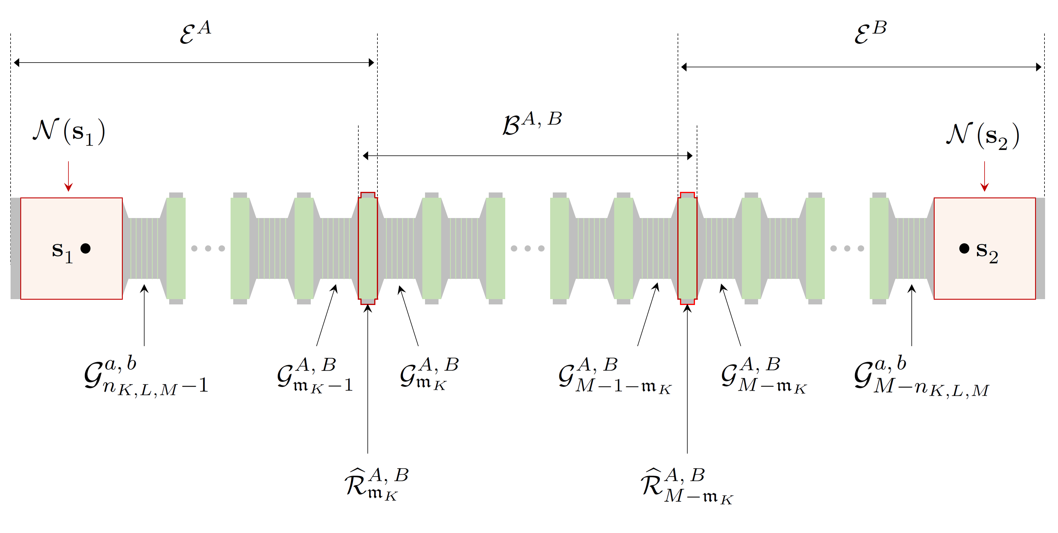
Figure 9.1. 3D typical configurations for the Ising model. Suppose that $q=2$, $A=\{1\}$, and $B=\{2\}$ (one can compare this figure with Figure 7.2). The given figure provides an illustration of the complete structure of the set $\widehat{\mathcal{N}}(\mathcal{S})$. This characterization is verified in Proposition 9.6. We take bulk ones only from $\mathfrak{m}_{K}$ to $M-\mathfrak{m}_{K}$ instead of $n_{K,\,L,\,M}$ (cf. (6.22)) to $M-n_{K,\,L,\,M}$ since we do not know the exact value of $n_{K,\,L,\,M}$. Because of this, the structure of the edge typical configurations is a little bit more complicated than in the 2D case.

For $a,\,b\in S$ and $i\in\llbracket 0,\,M\rrbracket$, we define

$$\widehat{\mathcal{R}}_{i}^{a,\,b}=\widehat{\mathcal{N}}(\mathcal{R}_{i}^{a,\,b}\,;\,\mathcal{G}^{a,\,b})\;.$$ (9.1)

We also define

$$\widehat{\mathcal{R}}_{i}^{A,\,B}=\widehat{\mathcal{N}}(\mathcal{R}_{i}^{A,\,B}\,;\,\mathcal{G}^{A,\,B})\;\;\;\;;\;i\in\llbracket 0,\,M\rrbracket\;.$$

Remark 9.1.

For $i\in\llbracket\mathfrak{m}_{K},\,M-\mathfrak{m}_{K}\rrbracket$, we have that

$$\widehat{\mathcal{R}}_{i}^{A,\,B}=\bigcup_{a\in A,\,b\in B}\widehat{\mathcal{R}}_{i}^{a,\,b}\;.$$

To check this, it suffices to check $\widehat{\mathcal{N}}(\mathcal{R}_{i}^{a,\,b}\,;\,\mathcal{G}^{a,\,b})=\widehat{\mathcal{N}}(\mathcal{R}_{i}^{a,\,b}\,;\,\mathcal{G}^{A,\,B})$ provided that $a\in A$ and $b\in B$. This follows from Lemma 8.3 since $\mathcal{R}_{i}^{a,\,b}$ cannot be connected to a configuration in $\mathcal{G}^{A,\,B}\setminus\mathcal{G}^{a,\,b}$ via a $\Gamma$-path in $\mathcal{X}\setminus\mathcal{G}^{a,\,b}$ by part (2) of Lemma 8.3.

Remark 9.2.

By Lemma 8.3, two sets $\widehat{\mathcal{R}}_{i}^{A,\,B}$ and $\widehat{\mathcal{R}}_{j}^{A,\,B}$ for different $i,\,j$ are disjoint if either $i\in\llbracket\mathfrak{m}_{K},\,M-\mathfrak{m}_{K}\rrbracket$ or $j\in\llbracket\mathfrak{m}_{K},\,M-\mathfrak{m}_{K}\rrbracket$. Moreover by Proposition 8.1, they are disjoint if $i\in\llbracket 0,\,\mathfrak{m}_{K}-1\rrbracket$ and $j\in\llbracket M-\mathfrak{m}_{K}+1,\,M\rrbracket$ or vice versa. On the other hand, they might be the same set if $i,\,j\in\llbracket 0,\,\mathfrak{m}_{K}-1\rrbracket$ or $i,\,j\in\llbracket M-\mathfrak{m}_{K}+1,\,M\rrbracket$. In particular, we have

$$\widehat{\mathcal{R}}_{0}^{A,\,B}=\widehat{\mathcal{R}}_{1}^{A,\,B}=\cdots=\widehat{\mathcal{R}}_{n_{K,L,M}-1}^{A,\,B}\;,$$

where $n_{K,\,L,\,M}$ is defined in (6.22). The same result holds for $\widehat{\mathcal{R}}_{i}^{a,\,b}$ instead of $\widehat{\mathcal{R}}_{i}^{A,\,B}$.

Now, we define the typical configurations. We recall Notation 7.4.

Definition 9.3 (Typical configurations).

For a proper partition $(A,\,B)$ of $S$, we define the typical configurations as follows.

• Bulk typical configurations: We define, for $a,\,b\in S$,

  $$\mathcal{B}^{a,\,b}=\mathcal{G}_{[\mathfrak{m}_{K},\,M-\mathfrak{m}_{K}-1]}^{a,\,b}\cup\widehat{\mathcal{R}}_{[\mathfrak{m}_{K},\,M-\mathfrak{m}_{K}]}^{a,\,b}\;,$$

  and then define

  $$\mathcal{B}^{A,\,B}=\bigcup_{a\in A}\bigcup_{b\in B}\mathcal{B}^{a,\,b}=\mathcal{G}_{[\mathfrak{m}_{K},\,M-\mathfrak{m}_{K}-1]}^{A,\,B}\cup\widehat{\mathcal{R}}_{[\mathfrak{m}_{K},\,M-\mathfrak{m}_{K}]}^{A,\,B}\;,$$ (9.2)

  where the second identity holds because of Remark 9.1. A configuration belonging to $\mathcal{B}^{A,\,B}$ is called a bulk typical configuration between $\mathcal{S}(A)$ and $\mathcal{S}(B)$.

• Edge typical configurations: We define

  $$\mathcal{E}^{A}=\mathcal{G}_{\mathfrak{m}_{K}-1}^{A,\,B}\cup\widehat{\mathcal{R}}_{[0,\,\mathfrak{m}_{K}]}^{A,\,B}\;\;\;\;\text{and}\;\;\;\;\mathcal{E}^{B}=\mathcal{G}_{M-\mathfrak{m}_{K}}^{A,\,B}\cup\widehat{\mathcal{R}}_{[M-\mathfrak{m}_{K},\,M]}^{A,\,B}\;.$$ (9.3)

  Finally, we define $\mathcal{E}^{A,\,B}=\mathcal{E}^{A}\cup\mathcal{E}^{B}$. A configuration belonging to $\mathcal{E}^{A,\,B}$ is called an edge typical configuration between $\mathcal{S}(A)$ and $\mathcal{S}(B)$.

Later in Proposition 9.6, we shall show that $\mathcal{B}^{A,\,B}\cup\mathcal{E}^{A,\,B}=\widehat{\mathcal{N}}(\mathcal{S})$ and hence all relevant configurations in the analysis of metastable behavior between $\mathcal{S}(A)$ and $\mathcal{S}(B)$ belong to either $\mathcal{B}^{A,\,B}$ or $\mathcal{E}^{A,\,B}$.

Remark 9.4.

Since $\mathcal{R}_{0}^{A,\,B}=\mathcal{S}(A)$ and $\mathcal{R}_{M}^{A,\,B}=\mathcal{S}(B)$ (cf. (6.7)), we can readily observe that $\mathcal{S}(A)\subseteq\mathcal{E}^{A}$ and $\mathcal{S}(B)\subseteq\mathcal{E}^{B}$.

9.2. Properties of typical configurations

In this subsection, we analyze some properties of the edge and bulk typical configurations. In fact, we have to take $K$ large enough (i.e., $K\geq 2829$) in order to get the structural properties of edge and bulk typical configurations given in the current section.

The first property asserts that $\mathcal{E}^{A}$ and $\mathcal{E}^{B}$ are disjoint.

Proposition 9.5.

The two sets $\mathcal{E}^{A}$ and $\mathcal{E}^{B}$ are disjoint.

Proof.

By part (2) of Lemma 8.3 (cf. Remark 9.2), the set $\widehat{\mathcal{R}}_{\mathfrak{m}_{K}}^{A,\,B}$ is disjoint with $\mathcal{E}^{B}$; similarly, the set $\widehat{\mathcal{R}}_{M-\mathfrak{m}_{K}}^{A,\,B}$ is disjoint with $\mathcal{E}^{A}$. It is direct from the definition that $\mathcal{G}_{\mathfrak{m}_{K}-1}^{A,\,B}$ and $\mathcal{G}_{M-\mathfrak{m}_{K}}^{A,\,B}$ are disjoint. By definition, $\mathcal{G}_{\mathfrak{m}_{K}-1}^{A,\,B},\,\mathcal{G}_{M-\mathfrak{m}_{K}}^{A,\,B}\subseteq\mathcal{G}^{A,\,B}$ are mutually disjoint with $\widehat{\mathcal{R}}_{[0,\,\mathfrak{m}_{K}]}^{A,\,B}$ and $\widehat{\mathcal{R}}_{[M-\mathfrak{m}_{K},\,M]}^{A,\,B}$. Hence, it suffices to prove that $\widehat{\mathcal{R}}_{[0,\,\mathfrak{m}_{K}-1]}^{A,\,B}$ and $\widehat{\mathcal{R}}_{[M-\mathfrak{m}_{K}+1,\,M]}^{A,\,B}$ are disjoint. Otherwise, we can take a configuration $\sigma$ such that

$$\sigma\in\widehat{\mathcal{R}}_{[0,\,\mathfrak{m}_{K}-1]}^{A,\,B}\cap\widehat{\mathcal{R}}_{[M-\mathfrak{m}_{K}+1,\,M]}^{A,\,B}\;.$$

Since $\sigma\in\widehat{\mathcal{R}}_{[0,\,\mathfrak{m}_{K}-1]}^{A,\,B}$, there exists a $\Gamma$-path in $\mathcal{X}\setminus\mathcal{G}^{A,\,B}$ (which is indeed a part of a canonical path) connecting $\sigma$ and $\mathcal{S}(A)$. Similarly, there exists a $\Gamma$-path in $\mathcal{X}\setminus\mathcal{G}^{A,\,B}$ connecting $\sigma$ and $\mathcal{S}(B)$. By concatenating them, we can find a $\Gamma$-path $(\omega_{t})_{t=0}^{T}$ in $\mathcal{X}\setminus\mathcal{G}^{A,\,B}$ connecting $\mathcal{S}(A)$ and $\mathcal{S}(B)$. This contradicts part (2) of Proposition 8.1. ∎

Now, we analyze the crucial features of the typical configurations. Note that this is a 3D version of Proposition 5.8.

Proposition 9.6.

For a proper partition $(A,\,B)$ of $S$, the following properties hold for the typical configurations.

1. It holds that $\mathcal{E}^{A}\cap\mathcal{B}^{A,\,B}=\widehat{\mathcal{R}}_{\mathfrak{m}_{K}}^{A,\,B}$ and $\mathcal{E}^{B}\cap\mathcal{B}^{A,\,B}=\widehat{\mathcal{R}}_{M-\mathfrak{m}_{K}}^{A,\,B}$.

2. We have $\mathcal{E}^{A,\,B}\cup\mathcal{B}^{A,\,B}=\widehat{\mathcal{N}}(\mathcal{S})$.

Proof.

(1) It suffices to prove the first identity, as the second one follows similarly. One can observe that the set $\mathcal{G}_{\mathfrak{m}_{K}-1}^{A,\,B}\subseteq\mathcal{G}^{A,\,B}$ is disjoint with $\mathcal{B}^{A,\,B}$ from (9.2), and the set $\mathcal{G}_{[\mathfrak{m}_{K},\,M-\mathfrak{m}_{K}-1]}^{A,\,B}\subseteq\mathcal{G}^{A,\,B}$ is disjoint with $\mathcal{E}^{A}$ in view of the expression (9.3). Therefore, by (9.2) and (9.3), we get

$$\mathcal{E}^{A}\cap\mathcal{B}^{A,\,B}=\widehat{\mathcal{R}}_{[0,\,\mathfrak{m}_{K}]}^{A,\,B}\cap\widehat{\mathcal{R}}_{[\mathfrak{m}_{K},\,M-\mathfrak{m}_{K}]}^{A,\,B}\;.$$ (9.4)

By Lemma 8.3, the two sets $\mathcal{R}_{[0,\,\mathfrak{m}_{K}-1]}^{A,\,B}$ and $\mathcal{R}_{[\mathfrak{m}_{K},\,M-\mathfrak{m}_{K}]}^{A,\,B}$ cannot be connected by a $\Gamma$-path in $\mathcal{X}\setminus\mathcal{G}^{A,\,B}$, and hence $\mathcal{\widehat{\mathcal{R}}}_{[0,\,\mathfrak{m}_{K}-1]}^{A,\,B}$ and $\mathcal{\widehat{\mathcal{R}}}_{[\mathfrak{m}_{K},\,M-\mathfrak{m}_{K}]}^{A,\,B}$ are disjoint. Therefore, we have

$$\widehat{\mathcal{R}}_{[0,\,\mathfrak{m}_{K}]}^{A,\,B}\cap\widehat{\mathcal{R}}_{[\mathfrak{m}_{K},\,M-\mathfrak{m}_{K}]}^{A,\,B}=\widehat{\mathcal{R}}_{\mathfrak{m}_{K}}^{A,\,B}\cap\widehat{\mathcal{R}}_{[\mathfrak{m}_{K},\,M-\mathfrak{m}_{K}]}^{A,\,B}=\widehat{\mathcal{R}}_{\mathfrak{m}_{K}}^{A,\,B}\;.$$ (9.5)

The proof is completed by (9.4) and (9.5).

(2) We will first prove that

$$\widehat{\mathcal{N}}(\mathcal{S})=\widehat{\mathcal{N}}(\mathcal{N}(\mathcal{R}_{[0,\,M]}^{A,\,B})\cup\mathcal{G}^{A,\,B})\;.$$ (9.6)

Since it is immediate that $\mathcal{S}$ is a subset of the right-hand side, we have $\widehat{\mathcal{N}}(\mathcal{S})\subseteq\widehat{\mathcal{N}}(\mathcal{N}(\mathcal{R}_{[0,\,M]}^{A,\,B})\cup\mathcal{G}^{A,\,B})$. On the other hand, since $\mathcal{N}(\mathcal{R}_{[0,\,M]}^{A,\,B})\cup\mathcal{G}^{A,\,B}\subseteq\widehat{\mathcal{N}}(\mathcal{S})$ clearly holds, we also have $\widehat{\mathcal{N}}(\mathcal{N}(\mathcal{R}_{[0,\,M]}^{A,\,B})\cup\mathcal{G}^{A,\,B})\subseteq\widehat{\mathcal{N}}(\mathcal{S})$. This proves (9.6). Since the sets $\mathcal{N}(\mathcal{R}_{[0,\,M]}^{A,\,B})$ and $\mathcal{G}^{A,\,B}$ are disjoint by Lemma 7.6, we can apply Lemmas 4.2 and 7.6 to deduce

$$\widehat{\mathcal{N}}(\mathcal{S}) =\widehat{\mathcal{N}}(\mathcal{N}(\mathcal{R}_{[0,\,M]}^{A,\,B})\,;\,\mathcal{G}^{A,\,B})\cup\widehat{\mathcal{N}}(\mathcal{G}^{A,\,B}\,;\,\mathcal{N}(\mathcal{R}_{[0,\,M]}^{A,\,B}))\;.$$

$$=\widehat{\mathcal{N}}(\mathcal{R}_{[0,\,M]}^{A,\,B}\,;\,\mathcal{G}^{A,\,B})\cup\mathcal{G}^{A,\,B}=\widehat{\mathcal{R}}_{[0,\,M]}^{A,\,B}\cup\mathcal{G}^{A,\,B}\;.$$

This completes the proof since by (7.3), (9.2) and (9.3), we have $\mathcal{E}^{A,\,B}\cup\mathcal{B}^{A,\,B}=\mathcal{G}^{A,\,B}\cup\widehat{\mathcal{R}}_{[0,\,M]}^{A,\,B}$. ∎

9.3. Structure of edge typical configurations

As in the 2D case [25, Sections 6.4 and 6.5], we analyze the structure of edge typical configurations.

We remark that we fixed a proper partition $(A,\,B)$ of $S$. Decompose

$$\mathcal{E}^{A}=\mathcal{O}^{A}\cup\mathcal{I}^{A}$$ (9.7)

where

$$\mathcal{O}^{A}=\{\sigma\in\mathcal{E}^{A}:H(\sigma)=\Gamma\}\;\;\;\;\text{and}\;\;\;\;\mathcal{I}^{A}=\{\sigma\in\mathcal{E}^{A}:H(\sigma)<\Gamma\}\;.$$

We now take a subset $\overline{\mathcal{I}}^{A}$ of $\mathcal{I}^{A}$ so that we can decompose $\mathcal{I}^{A}$ into the following disjoint union:

$$\mathcal{I}^{A}=\bigcup_{\sigma\in\overline{\mathcal{I}}^{A}}\mathcal{N}(\sigma)\;.$$

Consequently, we get the following decomposition of $\mathcal{E}^{A}$:

$$\mathcal{E}^{A}=\mathcal{O}^{A}\cup\Big{(}\,\bigcup_{\sigma\in\overline{\mathcal{I}}^{A}}\mathcal{N}(\sigma)\,\Big{)}\;.$$ (9.8)

Notation 9.7.

For $\sigma\in\mathcal{I}^{A}$, we denote by $\overline{\sigma}\in\overline{\mathcal{I}}^{A}$ the unique configuration satisfying $\sigma\in\mathcal{N}(\overline{\sigma})$.

By part (1) of Lemma 8.3, for $\sigma,\,\sigma^{\prime}\in\mathcal{R}_{\mathfrak{m}_{K}}^{A,\,B}$, the two sets $\mathcal{N}(\sigma)$ and $\mathcal{N}(\sigma^{\prime})$ are disjoint. By a similar reasoning, we know that for any $\sigma\in\mathcal{R}_{\mathfrak{m}_{K}}^{A,\,B}$ and $a\in A$, the sets $\mathcal{N}(\sigma)$ and $\mathcal{N}(\mathbf{s}_{a})$ are disjoint. Thus, we can assume that

$$\mathcal{R}_{\mathfrak{m}_{K}}^{A,\,B}\cup\mathcal{S}(A)\subseteq\overline{\mathcal{I}}^{A}\;.$$ (9.9)

The following construction of an auxiliary Markov chain is an analogue of [25, Definition 6.20].

Definition 9.8.

For a proper partition $(A,\,B)$ of $S$, we define a Markov chain $Z^{A}(\cdot)$ on $\overline{\mathcal{I}}^{A}\cup\mathcal{O}^{A}$.

• (Graph) We define the graph structure $\mathscr{G}^{A}=(\mathscr{V}^{A},\,\mathscr{E}^{A})$ for $\mathscr{V}^{A}=\mathcal{O}^{A}\cup\overline{\mathcal{I}}^{A}$. The edge set $\mathscr{E}^{A}$ is defined by declaring that $\{\sigma,\,\sigma^{\prime}\}\in\mathscr{E}^{A}$ for $\sigma,\,\sigma^{\prime}\in\mathscr{V}^{A}$ if

  $$\begin{cases}\sigma,\,\sigma^{\prime}\in\mathcal{O}^{A}\text{ and }\sigma\sim\sigma^{\prime}\text{ or}\\ \sigma\in\mathcal{O}^{A}\;,\;\sigma^{\prime}\in\overline{\mathcal{I}}^{A}\;,\;\text{ and }\sigma\sim\zeta\text{ for some }\zeta\in\mathcal{N}(\sigma^{\prime})\;.\end{cases}$$

• (Markov chain) We first define a rate $r^{A}:\mathscr{V}^{A}\times\mathscr{V}^{A}\rightarrow[0,\,\infty)$. If $\{\sigma,\,\sigma^{\prime}\}\notin\mathscr{E}^{A}$, we set $r^{A}(\sigma,\,\sigma^{\prime})=0$, and if $\{\sigma,\,\sigma^{\prime}\}\in\mathscr{E}^{A}$, we set

  $$r^{A}(\sigma,\,\sigma^{\prime})=\begin{cases}1&\text{if }\sigma,\,\sigma^{\prime}\in\mathcal{O}^{A}\;,\\ |\{\zeta\in\mathcal{N}(\sigma):\zeta\sim\sigma^{\prime}\}|&\text{if }\sigma\in\overline{\mathcal{I}}^{A}\;,\;\sigma^{\prime}\in\mathcal{O}^{A}\;,\\ |\{\zeta\in\mathcal{N}(\sigma^{\prime}):\zeta\sim\sigma\}|&\text{if }\sigma\in\mathcal{O}^{A}\;,\;\sigma^{\prime}\in\overline{\mathcal{I}}^{A}\;.\end{cases}$$ (9.10)

  We now let $(Z^{A}(t))_{t\geq 0}$ be the continuous-time Markov chain on $\mathscr{V}^{A}$ with rate $r^{A}(\cdot,\,\cdot)$. Note that the uniform distribution on $\mathscr{V}^{A}$ is the invariant measure for the chain $Z^{A}(\cdot)$, and indeed this chain is reversible with respect to this measure.

• (Potential-theoretic objects) Denote by $L^{A}$, $h_{\cdot,\,\cdot}^{A}(\cdot)$, and $\mathrm{cap}^{A}(\cdot,\,\cdot)$ the generator, equilibrium potential, and capacity with respect to the Markov chain $Z^{A}(\cdot)$, respectively.

We now give three important propositions regarding the objects constructed above. These propositions play fundamental roles in the construction of the test function on the edge typical configurations.

We remark from (9.9) that $\mathcal{S}(A),\,\mathcal{R}_{\mathfrak{m}_{K}}^{A,\,B}\subseteq\overline{\mathcal{I}}^{A}\subseteq\mathscr{V}^{A}.$ Potential-theoretic objects between these two sets are crucially used in our discussion. We define

$$\mathfrak{e}(A)=\frac{1}{|\mathscr{V}^{A}|\,\mathrm{cap}^{A}(\mathcal{S}(A),\,\mathcal{R}_{\mathfrak{m}_{K}}^{A,\,B})}\;.$$ (9.11)

For $n\in\llbracket 1,\,q-1\rrbracket$ (with a slight abuse of notation) we can write

$$\mathfrak{e}(n)=\frac{1}{|\mathscr{V}^{A_{n}}|\,\mathrm{cap}^{A_{n}}(\mathcal{S}(A_{n}),\,\mathcal{R}_{\mathfrak{m}_{K}}^{A_{n},\,B_{n}})}\;,$$ (9.12)

where $A_{n}=\{1,\,\dots,\,n\}$ and $B_{n}=\{n+1,\,\dots,\,q\}$. Since $\mathfrak{e}(A)$ depends on $A$ only through $|A|$, it holds that $\mathfrak{e}(A)=\mathfrak{e}(|A|)$. We next derive a rough bound of $\mathfrak{e}(n)$ via the Thomson principle. We refer to e.g., [12] for the flow structure and the Thomson principle.

Proposition 9.9.

For all $n\in\llbracket 1,\,q-1\rrbracket$, we have that $\mathfrak{e}(n)\leq\frac{1}{K^{1/3}}$.

Proof.

We recall that an anti-symmetric function $\phi:\mathscr{V}^{A}\times\mathscr{V}^{A}\to\mathbb{R}$ is called a flow associated with the Markov chain $Z^{A}(\cdot)$, provided that $\phi(x,\,y)\neq 0$ if and only if $\{x,\,y\}\in\mathscr{E}^{A}$. For each flow $\phi$, the associated flow norm is defined by

$$\|\phi\|^{2}:=\sum_{\{x,\,y\}\subseteq\mathscr{V}^{A}:\,\{x,\,y\}\in\mathscr{E}^{A}}\frac{\phi(x,\,y)^{2}}{|\mathscr{V}^{A}|^{-1}\,r^{A}(x,\,y)}\;.$$

For each $x\in\mathscr{V}^{A}$, the divergence of a flow $\phi$ at $x$ is defined by

$$(\mathrm{div}\,\phi)(x):=\sum_{y\in\mathscr{V}^{A}}\phi(x,\,y)\;.$$

Finally, for two disjoint non-empty subsets $\mathcal{U},\,\mathcal{V}$ of $\mathscr{V}^{A}$, a flow $\phi$ is called a unit flow from $\mathcal{U}$ to $\mathcal{V}$ if

$$\sum_{x\in\mathcal{U}}(\mathrm{div}\,\phi)(x)=-\sum_{x\in\mathcal{V}}(\mathrm{div}\,\phi)(x)=1\;\;\;\;\text{and}\;\;\;\;(\mathrm{div}\,\phi)(z)=0\text{ for all }z\notin\mathcal{U}\cup\mathcal{V}\;.$$

Then, by the Thomson principle (cf. [12, Theorem 7.37]), for any unit flow $\psi$ from $\mathcal{S}(A)$ to $\mathcal{R}_{\mathfrak{m}_{K}}^{A,\,B}$, we have

$$\mathrm{cap}^{A}(\mathcal{S}(A),\,\mathcal{R}_{\mathfrak{m}_{K}}^{A,\,B})\geq\frac{1}{\|\psi\|^{2}}\;.$$ (9.13)

We shall construct below a unit flow $\psi$ from $\mathcal{S}(A)$ to $\mathcal{R}_{\mathfrak{m}_{K}}^{A,\,B}$ that satisfies

$$\|\psi\|^{2}<\frac{\mathfrak{m}_{K}\,|\mathscr{V}^{A}|}{2M}\;.$$ (9.14)

Then, by combining (9.13) and (9.14), we have (recalling the definition (6.20) of $\mathfrak{m}_{K}$)

$$\mathrm{cap}^{A}(\mathcal{S}(A),\,\mathcal{R}_{\mathfrak{m}_{K}}^{A,\,B})\geq\frac{1}{\|\psi\|^{2}}>\frac{2M}{|\mathscr{V}^{A}|\,\mathfrak{m}_{K}}\geq\frac{K^{1/3}}{|\mathscr{V}^{A}|}\;.$$

Recalling the definition (9.11), this completes the proof.

Now, it remains to construct a unit flow $\psi$ from $\mathcal{S}(A)$ to $\mathcal{R}_{\mathfrak{m}_{K}}^{A,\,B}$ satisfying bound (9.14). To this end, let us first fix $a\in A$ and $b\in B$. Define

$$i_{K,\,L,\,M}=\max\,\{m\geq 1:\Phi(\mathcal{S}(A),\,\mathcal{R}_{m}^{A,\,B})<\Gamma\}\;.$$ (9.15)

By Corollary 8.5, we know that $i_{K,\,L,\,M}<\mathfrak{m}_{K}$.

Let us start by fixing $P,\,Q\in\mathfrak{S}_{M}$ such that $P\prec Q$, $Q\setminus P=\{m\}$, $i_{K,\,L,\,M}\leq|P|<|Q|\leq\mathfrak{m}_{K}$, $a\in A$, and $b\in B$. Then, we first define a flow $\psi_{P,\,Q}$ connecting $\overline{\sigma}_{P}^{a,\,b}=\overline{\sigma_{P}^{a,\,b}}$ and $\overline{\sigma}_{Q}^{a,\,b}=\overline{\sigma_{Q}^{a,\,b}}$ (cf. Notation 9.7). First, we set

$$\psi_{P,\,Q}(\sigma,\,\zeta)=-\psi_{P,\,Q}(\zeta,\,\sigma)=\frac{1}{2KLM}$$ (9.16)

if $\sigma,\,\zeta\in\mathcal{C}_{P,\>Q}^{a,\,b}$ satisfy, for some $\ell\in\mathbb{T}_{L}$, $k\in\mathbb{T}_{K}$, $v\in\llbracket 1,\,L-2\rrbracket$, and $h\in\llbracket 1,\,K-2\rrbracket$,

$$\begin{cases}\sigma^{(m)}=\xi_{\ell,\,v}^{a,\,b}\;\;\text{and}\;\;\zeta^{(m)}=\xi_{\ell,\,v;\,k,\,1}^{a,\,b,\,+}\;\;\;\;\text{or}\;,\\ \sigma^{(m)}=\xi_{\ell,\,v;\,k,\,h}^{a,\,b,\,+}\;\;\text{and}\;\;\zeta^{(m)}=\xi_{\ell,\,v;\,k,\,h+1}^{a,\,b,\,+}\;\;\;\;\text{or\;,}\\ \sigma^{(m)}=\xi_{\ell,\,v;\,k,\,K-1}^{a,\,b,\,+}\;\;\text{and}\;\;\zeta^{(m)}=\xi_{\ell,\,v+1}^{a,\,b}\;.\end{cases}$$ (9.17)

Now, we claim that all configurations that appear in (9.17) except for the ones corresponding to $\xi_{\ell,\,1}^{a,\,b}$ and $\xi_{\ell,\,L-1}^{a,\,b}$ belong to $\mathscr{V}^{A}$. To check this, observe first that if the $m$-th floor of $\sigma\in\mathcal{C}_{P,\>Q}^{a,\,b}$ is of the form $\sigma^{(m)}=\xi_{\ell,\,v\,;\,k,\,h}^{a,\,b,\,+}$, we have $H(\sigma)=\Gamma$ and hence $\sigma\in\mathcal{O}^{A}$. On the other hand, if the $m$-th floor of $\sigma\in\mathcal{C}_{P,\>Q}^{a,\,b}$ is of the form $\sigma^{(m)}=\xi_{\ell,\,v}^{a,\,b}$ for $v\in\llbracket 2,\,L-2\rrbracket$, we have $H(\sigma)=\Gamma-2$ and moreover $\mathcal{N}(\sigma)=\{\sigma\}$. This implies that $\sigma\in\overline{\mathcal{I}}^{A}$. This proves the claim. On the other hand, since if $\sigma^{(m)}=\xi_{\ell,\,1}^{a,\,b}$ then $\sigma\in\mathcal{N}(\sigma_{P}^{a,\,b})$, and if $\sigma^{(m)}=\xi_{\ell,\,L-1}^{a,\,b}$ then $\sigma\in\mathcal{N}(\sigma_{Q}^{a,\,b})$ (cf. the canonical paths provide $(\Gamma-1)$-paths), we can replace the configurations corresponding to $\xi_{\ell,\,1}^{a,\,b}$ and $\xi_{\ell,\,L-1}^{a,\,b}$ that appear in (9.17) with $\overline{\sigma}_{P}^{a,\,b}$ and $\overline{\sigma}_{Q}^{a,\,b}$, respectively, to get a flow connecting $\overline{\sigma}_{P}^{a,\,b}$ and $\overline{\sigma}_{Q}^{a,\,b}$. We remark that we may have $\overline{\sigma}_{P}^{a,\,b}=\overline{\sigma}_{Q}^{a,\,b}$.

We deduce from the definition of the flow norm that

$$\|\psi_{P,\,Q}\|^{2}=\frac{|\mathscr{V}^{A}|}{(2KLM)^{2}}\times K^{2}L(L-2)<\frac{|\mathscr{V}^{A}|}{4M^{2}}\;,$$ (9.18)

where $K^{2}L(L-2)$ is the number of edges that appear in (9.17). Next, we define

$$\psi=\sum_{r=i_{K,L,M}}^{\mathfrak{m}_{K}-1}\,\sum_{P,\,Q\in\mathfrak{S}_{M}:\,|P|=r,\,P\prec Q}\psi_{P,\,Q}\;.$$

Notice from (9.15) that a configuration of the form $\overline{\sigma}_{P,\,Q}^{a,\,b}$ with $|P|=i_{K,\,L,\,M}$ is indeed an element of $\mathcal{S}(A)$. Then, from the definition (9.16), we can readily check that $\psi(x)=0$ for all $x\notin\mathcal{S}(A)\cup\mathcal{R}_{\mathfrak{m}_{K}}^{A,\,B}$ (by using the fact that the flow on each edge has a constant magnitude $\frac{1}{2KLM}$), and moreover it holds that (cf. (9.9))

$$\sum_{x\in\mathcal{S}(A)}\sum_{y\in\mathscr{V}^{A}}\psi(x,\,y)=1\;.$$ (9.19)

Indeed, to prove the last assertion, it suffices to observe that

$$\sum_{x\in\mathcal{S}(A)}\sum_{y\in\mathscr{V}^{A}}\psi(x,\,y) =\sum_{P,\,Q\in\mathfrak{S}_{M}:\,|P|=i_{K,L,M},\,P\prec Q}\,\sum_{\zeta\in\mathscr{V}^{A}:\,\overline{\sigma}_{P}^{a,b}\sim\zeta}\psi_{P,\,Q}(\overline{\sigma}_{P}^{a,\,b},\,\zeta)$$

$$=\frac{1}{2KLM}\times KL\times 2M=1\;,$$

where $KL$ is the number of configurations in $\mathcal{C}_{P,\,Q}^{a,\,b}$ connected to $\overline{\sigma}_{P}^{a,\,b}$, and $2M$ is the number of possible choices of $P$ and $Q$. Consequently, the flow $\psi$ is a unit flow from $\mathcal{S}(A)$ to $\mathcal{R}_{\mathfrak{m}_{K}}^{A,\,B}$.

Thus, it suffices to verify (9.14). Since the support of $\psi_{P,\,Q}$ (which is the collection of edges on which $\psi_{P,\,Q}$ is non-zero) for different pairs $(P,\,Q)$ are disjoint, we deduce from (9.18) that

$$\|\psi\|^{2}=\sum_{r=i_{K,L,M}}^{\mathfrak{m}_{K}-1}\,\sum_{P,\,Q\in\mathfrak{S}_{M}:\,|P|=r,\,P\prec Q}\|\psi_{P,\,Q}\|^{2}<\mathfrak{m}_{K}\times 2M\times\frac{|\mathscr{V}^{A}|}{4M^{2}}=\frac{\mathfrak{m}_{K}\,|\mathscr{V}^{A}|}{2M}\;,$$

and therefore $\psi$ satisfies (9.14). ∎

For simplicity, we write (cf. (9.9))

$$\mathfrak{h}^{A}(\cdot)=h_{\mathcal{S}(A),\,\mathcal{R}_{\mathfrak{m}_{K}}^{A,B}}^{A}(\cdot)$$ (9.20)

where $h^{A}$ is the equilibrium potential defined in Definition 9.8. This function is a fundamental object in the construction of the test function in Section 10.

Proposition 9.10.

For $\sigma\in\widehat{\mathcal{R}}_{\mathfrak{m}_{K}}^{A,\,B}\cap\mathcal{O}^{A}\subseteq\mathscr{V}^{A}$, we have $\mathfrak{h}^{A}(\sigma)=0$.

Proof.

We fix $\sigma\in\widehat{\mathcal{R}}_{\mathfrak{m}_{K}}^{A,\,B}\cap\mathcal{O}^{A}$. It suffices to prove that any $\Gamma$-path $(\omega_{t})_{t=0}^{T}$ from $\sigma$ to $\mathcal{S}(A)$ must visit $\mathcal{N}(\mathcal{R}_{\mathfrak{m}_{K}}^{A,\,B})$. Suppose first that the path $(\omega_{t})_{t=0}^{T}$ does not visit $\mathcal{G}^{A,\,B}$. Since $\sigma\in\mathcal{\widehat{R}}_{\mathfrak{m}_{K}}^{A,\,B}$, there exists a $\Gamma$-path in $\mathcal{X}\setminus\mathcal{G}^{A,\,B}$ connecting $\mathcal{R}_{\mathfrak{m}_{K}}^{A,\,B}$ and $\sigma$, and therefore by concatenating this path with $(\omega_{t})_{t=0}^{T}$, we get a $\Gamma$-path in $\mathcal{X}\setminus\mathcal{G}^{A,\,B}$ connecting $\mathcal{R}_{\mathfrak{m}_{K}}^{A,\,B}$ and $\mathcal{S}(A)$. This contradicts part (2) of Lemma 8.3. Thus, the path $(\omega_{t})_{t=0}^{T}$ must visit $\mathcal{G}^{A,\,B}$ and we let

$$t_{0}=\min\,\{t:\omega_{t}\in\mathcal{G}^{A,\,B}\}\;.$$

By part (2) of Lemma 7.5, we have $\omega_{t_{0}-1}\in\mathcal{N}(\mathcal{R}_{[\mathfrak{m}_{K}-1,\,M-\mathfrak{m}_{K}+1]}^{A,\,B})$. If $\omega_{t_{0}-1}\in\mathcal{N}(\mathcal{R}_{i}^{A,\,B})$ for some $i\in\llbracket\mathfrak{m}_{K}-1,\,M-\mathfrak{m}_{K}+1\rrbracket\setminus\{\mathfrak{m}_{K}\}$, then $(\omega_{t})_{t=0}^{t_{0}-1}$ induces a $\Gamma$-path from $\mathcal{R}_{\mathfrak{m}_{K}}^{A,\,B}$ from $\mathcal{R}_{i}^{A,\,B}$ avoiding $\mathcal{G}^{A,\,B}$, which contradicts part (2) of Lemma 8.3. Hence, we can conclude that $\omega_{t_{0}-1}\in\mathcal{N}(\mathcal{R}_{\mathfrak{m}_{K}}^{A,\,B})$, as desired. ∎

Remark 9.11.

The previous proposition implies that configurations $\sigma$ that belong to $\widehat{\mathcal{R}}_{\mathfrak{m}_{K}}^{A,\,B}\cap\mathcal{O}^{A}$ are dead-ends attached to $\mathcal{N}(\mathcal{R}_{\mathfrak{m}_{K}}^{A,\,B})$ (cf. grey protuberances attached to green boxes in Figures 7.2 and 9.1).

The next proposition highlights the fact that the auxiliary process $Z^{A}(\cdot)$ defined in Definition 9.8 approximates the behavior of the Metropolis–Hastings dynamics at the edge typical configurations.

Proposition 9.12.

Define a projection map $\Pi^{A}:\mathcal{E}^{A}\rightarrow\mathscr{V}^{A}$ by (cf. Notation 9.7)

$$\Pi^{A}(\sigma)=\begin{cases}\overline{\sigma}&\text{if }\sigma\in\mathcal{I}^{A}\;,\\ \sigma&\text{if }\sigma\in\mathcal{O}^{A}\;.\end{cases}$$

Then, there exists $C=C(K,\,L,\,M)>0$ such that

1. for $\sigma_{1},\,\sigma_{2}\in\mathcal{O}^{A}$, we have

   $$\Big{|}\,\frac{1}{q}e^{-\Gamma\beta}\,r^{A}(\Pi^{A}(\sigma_{1}),\,\Pi^{A}(\sigma_{2}))-\mu_{\beta}(\sigma_{1})\,r_{\beta}(\sigma_{1},\,\sigma_{2})\,\Big{|}\leq Ce^{-(\Gamma+1)\beta}\;,$$ (9.21)

2. for $\sigma_{1}\in\mathcal{O}^{A}$ and $\sigma_{2}\in\overline{\mathcal{I}}^{A}$, we have

   $$\Big{|}\,\frac{1}{q}e^{-\Gamma\beta}\,r^{A}(\Pi^{A}(\sigma_{1}),\,\Pi^{A}(\sigma_{2}))-\sum_{\zeta\in\mathcal{N}(\sigma_{2})}\mu_{\beta}(\sigma_{1})\,r_{\beta}(\sigma_{1},\,\zeta)\,\Big{|}\leq Ce^{-(\Gamma+1)\beta}\;.$$ (9.22)

Proof.

(1) Suppose that $\sigma_{1},\,\sigma_{2}\in\mathcal{O}^{A}$. Since if $\sigma_{1}\not\sim\sigma_{2}$ then the left-hand side of (9.21) is $0$, we may assume that $\sigma_{1}\sim\sigma_{2}$. In this case, $\{\sigma_{1},\,\sigma_{2}\}\in\mathscr{E}^{A}$, and thus

$$\Big{|}\,\frac{1}{q}e^{-\Gamma\beta}\,r^{A}(\Pi^{A}(\sigma_{1}),\,\Pi^{A}(\sigma_{2}))-\mu_{\beta}(\sigma_{1})\,r_{\beta}(\sigma_{1},\,\sigma_{2})\,\Big{|}=\Big{|}\,\frac{1}{q}e^{-\Gamma\beta}-\frac{1}{Z_{\beta}}e^{-\Gamma\beta}\,\Big{|}$$

since $\mu_{\beta}(\sigma_{1})=\mu_{\beta}(\sigma_{2})=\frac{1}{Z_{\beta}}e^{-\Gamma\beta}$ by the definition of $\mathcal{O}^{A}$. By (2.5), the right-hand side of the previous display is $O_{\beta}(e^{-(\Gamma+1)\beta})$.

(2) Let $\sigma_{1}\in\mathcal{O}^{A}$ and $\sigma_{2}\in\overline{\mathcal{I}}^{A}$. Similarly, we may assume that $\sigma_{1}\sim\sigma_{2}$. Then, we can write

$$\Big{|}\,\frac{1}{q}e^{-\Gamma\beta}\,r^{A}(\Pi^{A}(\sigma_{1}),\,\Pi^{A}(\sigma_{2}))-\sum_{\zeta\in\mathcal{N}(\sigma_{2})}\mu_{\beta}(\sigma_{1})\,r_{\beta}(\sigma_{1},\,\zeta)\,\Big{|}$$

$$=\Big{|}\,\frac{1}{q}e^{-\Gamma\beta}\,|\{\zeta\in\mathcal{N}(\sigma_{2}):\zeta\sim\sigma_{1}\}|-\sum_{\zeta\in\mathcal{N}(\sigma_{2}):\,\zeta\sim\sigma_{1}}\min\,\{\mu_{\beta}(\sigma_{1}),\,\mu_{\beta}(\zeta)\}\,\Big{|}$$

$$=|\{\zeta\in\mathcal{N}(\sigma_{2}):\zeta\sim\sigma_{1}\}|\times\Big{|}\,\frac{1}{q}e^{-\Gamma\beta}-\frac{1}{Z_{\beta}}e^{-\Gamma\beta}\,\Big{|}\;,$$

since $\min\,\{\mu_{\beta}(\sigma_{1}),\,\mu_{\beta}(\zeta)\}=\mu_{\beta}(\sigma_{1})$ for all $\zeta\in\mathcal{N}(\sigma_{2})$. Again by (2.5), the last line is clearly bounded from above by $KL\times O_{\beta}(e^{-\Gamma\beta}\,e^{-\beta})=O_{\beta}(e^{-(\Gamma+1)\beta})$. This concludes the proof. ∎

9.4. Analysis of 3D transition paths

In this section, we finally define the collection of transition paths between ground states that appear in Theorem 2.9.

Definition 9.13 (Transition paths).

Write

$$\mathcal{H}^{A,\,B}=\mathcal{G}^{A,\,B}\cup\widehat{\mathcal{R}}_{[\mathfrak{m}_{K},\,M-\mathfrak{m}_{K}]}^{A,\,B}\;.$$ (9.23)

A path $(\omega_{t})_{t=0}^{T}$ is called a transition path between $\mathcal{S}(A)$ and $\mathcal{S}(B)$ if

$$\omega_{0}\in\widehat{\mathcal{N}}(\mathcal{S}(A)\,;\,\mathcal{G}^{A,\,B})\;,\;\omega_{T}\in\widehat{\mathcal{N}}(\mathcal{S}(B)\,;\,\mathcal{G}^{A,\,B})\;,\;\text{and}$$

$$\omega_{t}\in\mathcal{H}^{A,\,B}\text{ for all }t\in\llbracket 1,\,T-1\rrbracket\;.$$

In particular, we have $\omega_{0}\in\mathcal{N}(\mathcal{R}_{\mathfrak{m}_{K}-1}^{A,\,B})$, $\omega_{1}\in\mathcal{G}_{\mathfrak{m}_{K}-1}^{A,\,B}$, $\omega_{T-1}\in\mathcal{G}_{M-\mathfrak{m}_{K}}^{A,\,B}$, and $\omega_{T}\in\mathcal{N}(\mathcal{R}_{M-\mathfrak{m}_{K}+1}^{A,\,B})$ by part (1) of Lemma 7.5.

Remark 9.14.

The two sets $\widehat{\mathcal{N}}(\mathcal{S}(A)\,;\,\mathcal{G}^{A,\,B})$ and $\widehat{\mathcal{N}}(\mathcal{S}(B)\,;\,\mathcal{G}^{A,\,B})$ are disjoint thanks to part (2) of Proposition 8.1.

Now, we characterize all the optimal paths between ground states in terms of the transition paths.

Theorem 9.15.

Let $(\omega_{t})_{t=0}^{T}$ be a $\Gamma$-path connecting $\mathcal{S}(A)$ and $\mathcal{S}(B)$. Then, $(\omega_{t})_{t=0}^{T}$ has a transition path between $\mathcal{S}(A)$ and $\mathcal{S}(B)$ as a sub-path.

Proof.

Let $(\omega_{t})_{t=0}^{T}$ be a $\Gamma$-path connecting $\mathcal{S}(A)$ and $\mathcal{S}(B)$, and define

$$T^{\prime}=\min\,\{t:\omega_{t}\in\widehat{\mathcal{N}}(\mathcal{S}(B)\,;\,\mathcal{G}^{A,\,B})\}\;.$$

Then, define

$$t^{\prime}=\max\,\{t<T^{\prime}:\omega_{t}\in\widehat{\mathcal{N}}(\mathcal{S}(A)\,;\,\mathcal{G}^{A,\,B})\}\;.$$

We claim that the sub-path $(\omega_{t})_{t=t^{\prime}}^{T^{\prime}}$ is a transition path between $\mathcal{S}(A)$ and $\mathcal{S}(B)$. By part (1) of Lemma 7.5, we have

$$\omega_{t^{\prime}}\in\mathcal{N}(\mathcal{R}_{\mathfrak{m}_{K}-1}^{A,\,B})\;,\;\omega_{t^{\prime}+1}\in\mathcal{G}_{\mathfrak{m}_{K}-1}^{A,\,B}\;,\;\omega_{T^{\prime}-1}\in\mathcal{G}_{M-\mathfrak{m}_{K}}^{A,\,B}\;,\;\text{and}\;\omega_{T^{\prime}}\in\mathcal{N}(\mathcal{R}_{M-\mathfrak{m}_{K}+1}^{A,\,B})\;.$$

In particular, we get $\omega_{t^{\prime}+1},\,\omega_{T^{\prime}-1}\in\mathcal{H}^{A,\,B}$. To complete the proof of the claim, it suffices to check that, if $\sigma\in\mathcal{H}^{A,\,B}$ and $\zeta\notin\mathcal{H}^{A,\,B}$ satisfy $\sigma\sim\zeta$ and $H(\zeta)\leq\Gamma$, then $\zeta\in\mathcal{N}(\mathcal{R}_{\mathfrak{m}_{K}-1}^{A,\,B})\cup\mathcal{N}(\mathcal{R}_{M-\mathfrak{m}_{K}+1}^{A,\,B})$. To prove this, let us first assume that $\sigma\in\widehat{\mathcal{R}}_{i}^{a,\,b}$ for some $a\in A$, $b\in B$, and $i\in\llbracket\mathfrak{m}_{K},\,M-\mathfrak{m}_{K}\rrbracket$ (cf. (9.23)). Then, since $\zeta\notin\widehat{\mathcal{R}}_{i}^{a,\,b}$ and $H(\zeta)\leq\Gamma$, by the definition of $\widehat{\mathcal{R}}_{i}^{a,\,b}$ we must have $\zeta\in\mathcal{G}^{A,\,B}$, and hence we get a contradiction to the fact that $\zeta\notin\mathcal{H}^{A,\,B}$. Next, we assume that $\sigma\in\mathcal{G}_{i}^{A,\,B}$ for some $i\in\llbracket\mathfrak{m}_{K}-1,\,M-\mathfrak{m}_{K}\rrbracket$. Since $\zeta\in\mathcal{X}\setminus\mathcal{H}^{A,\,B}$, by Lemma 7.5, we have $\zeta\in\mathcal{N}(\mathcal{R}_{\mathfrak{m}_{K}-1}^{A,\,B})\cup\mathcal{N}(\mathcal{R}_{M-\mathfrak{m}_{K}+1}^{A,\,B})$. This completes the proof. ∎

Therefore, we can now say that the set $\mathcal{G}^{A,\,B}\cup\widehat{\mathcal{R}}_{[\mathfrak{m}_{K},\,M-\mathfrak{m}_{K}]}^{A,\,B}$ consists of a saddle plateau between $\mathcal{S}(A)$ and $\mathcal{S}(B)$, which is a huge set of saddle configurations.

Now, we can prove Theorem 2.9.

Proof of Theorem 2.9.

Denote by $\widehat{\tau}$ the hitting time of the set $\{\sigma\in\mathcal{X}:H(\sigma)\geq\Gamma+1\}$. Then, by the large deviation principle (e.g. [41, Theorem 3.2]), we have that

$$\mathbb{P}_{\mathbf{s}}^{\beta}\,[\widehat{\tau}<e^{\beta(\Gamma+1/2)}]=o_{\beta}(1)\;.$$

Hence, by part (1) of Theorem 2.7, we have that $\mathbb{P}_{\mathbf{s}}^{\beta}\,[\tau_{\breve{\mathbf{s}}}<\widehat{\tau}]=1-o_{\beta}(1)$. Thus, the conclusion of the theorem follows immediately from Theorem 9.15. ∎

10. Construction of Test Function

We fix in this section a proper partition $(A,\,B)$ of $S$. The main purpose of the current section is to construct a test function $\widetilde{h}=\widetilde{h}_{A,\,B}^{\beta}:\mathcal{X}\rightarrow\mathbb{R}$ that satisfies the two requirements of Proposition 3.2.

Notation 10.1.

Since the partition $(A,\,B)$ is fixed, we simply write $\mathfrak{b}=\mathfrak{b}(|A|)$, $\mathfrak{e}_{A}=\mathfrak{e}(|A|)$, $\mathfrak{e}_{B}=\mathfrak{e}(|B|)$, and $\mathfrak{c}=\mathfrak{c}(|A|)$ so that $\mathfrak{c}=\mathfrak{b}+\mathfrak{e}_{A}+\mathfrak{e}_{B}$ throughout the current section.

10.1. Construction of test function

We now define a function $\widetilde{h}:\mathcal{X}\rightarrow\mathbb{R}$ which indeed fulfills all requirements in Proposition 3.2, as we shall verify later.

Definition 10.2 (Test function).

We construct the test function $\widetilde{h}$ on $\mathcal{E}^{A,\,B}$, $\mathcal{B}^{A,\,B}$, and $(\mathcal{E}^{A,\,B}\cup\mathcal{B}^{A,\,B})^{c}$ separately. Recall Notation 9.7.

1. Construction of $\widetilde{h}$ on edge typical configurations $\mathcal{E}^{A,\,B}=\mathcal{E}^{A}\cup\mathcal{E}^{B}$.

   • For $\sigma\in\mathcal{E}^{A}$, we recall the decomposition (9.8) of $\mathcal{E}^{A}$ and define

     $$\widetilde{h}(\sigma)=\begin{cases}1-\frac{\mathfrak{e}_{A}}{\mathfrak{c}}(1-\mathfrak{h}^{A}(\sigma))&\text{if }\sigma\in\mathcal{O}^{A}\;,\\ 1-\frac{\mathfrak{e}_{A}}{\mathfrak{c}}(1-\mathfrak{h}^{A}(\overline{\sigma}))&\text{if }\sigma\in\mathcal{I}^{A}\;.\end{cases}$$ (10.1)

   • For $\sigma\in\mathcal{E}^{B}$, we similarly define

     $$\widetilde{h}(\sigma)=\begin{cases}\frac{\mathfrak{e}_{B}}{\mathfrak{c}}(1-\mathfrak{h}^{B}(\sigma))&\text{if }\sigma\in\mathcal{O}^{B}\;,\\ \frac{\mathfrak{e}_{B}}{\mathfrak{c}}(1-\mathfrak{h}^{B}(\overline{\sigma}))&\text{if }\sigma\in\mathcal{I}^{B}\;.\end{cases}$$ (10.2)

2. Construction of $\widetilde{h}$ on bulk typical configurations $\mathcal{B}^{A,\,B}$. Recall the 2D test function $\widetilde{h}^{\mathrm{2D}}$ explained in Proposition 5.11. We define the test function on each component of the decomposition (9.2) of $\mathcal{B}^{A,\,B}$.

   • Construction on $\mathcal{G}_{[\mathfrak{m}_{K},\,M-\mathfrak{m}_{K}-1]}^{A,\,B}$: Let us first fix $P,\,Q\in\mathfrak{S}_{M}$ such that $P\prec Q$ and $|P|\in\llbracket\mathfrak{m}_{K},\,M-\mathfrak{m}_{K}-1\rrbracket$. Write

     $$\mathcal{G}_{P,\,Q}^{A,\,B}=\bigcup_{a\in A,\,b\in B}\mathcal{G}_{P,\,Q}^{a,\,b}\;.$$

     The test function $\widetilde{h}$ is defined on $\mathcal{G}_{P,\,Q}^{A,\,B}$ by

     $$\widetilde{h}(\sigma)=\frac{1}{\mathfrak{c}}\,\Big{[}\,\frac{M-\mathfrak{m}_{K}-|P|-(1-\widetilde{h}^{\mathrm{2D}}(\sigma^{(m)}))}{M-2\mathfrak{m}_{K}}\mathfrak{b}+\mathfrak{e}_{B}\,\Big{]}\;\;\;\;;\;\sigma\in\mathcal{G}_{P,\,Q}^{A,\,B}\;,$$ (10.3)

     where $\{m\}=Q\setminus P$ so that $\sigma^{(m)}$ is a 2D gateway configuration between $\mathbf{s}_{a}^{\mathrm{2D}}$ and $\mathbf{s}_{b}^{\mathrm{2D}}$ for some $(a,\,b)\in A\times B$. Since $\mathcal{G}_{[\mathfrak{m}_{K},\,M-\mathfrak{m}_{K}-1]}^{A,\,B}$ can be decomposed into

     $$\mathcal{G}_{[\mathfrak{m}_{K},\,M-\mathfrak{m}_{K}-1]}^{A,\,B}=\bigcup_{i=\mathfrak{m}_{K}}^{M-\mathfrak{m}_{K}-1}\,\bigcup_{P,\,Q\in\mathfrak{S}_{M}:\,P\prec Q\,\text{and}\,|P|=i}\mathcal{G}_{P,\,Q}^{A,\,B}\;,$$

     we can combine the constructions (10.3) to define the test function on $\mathcal{G}_{[\mathfrak{m}_{K},\,M-\mathfrak{m}_{K}-1]}^{A,\,B}$.

   • Construction on $\widehat{\mathcal{R}}_{i}^{A,\,B}$ for $i\in\llbracket\mathfrak{m}_{K},\,M-\mathfrak{m}_{K}\rrbracket$: We set

     $$\widetilde{h}(\sigma)=\frac{1}{\mathfrak{c}}\,\Big{[}\,\frac{M-\mathfrak{m}_{K}-i}{M-2\mathfrak{m}_{K}}\mathfrak{b}+\mathfrak{e}_{B}\,\Big{]}\;\;\;\;;\;\sigma\in\widehat{\mathcal{R}}_{i}^{A,\,B}\;,$$ (10.4)

     so that the function $\widetilde{h}$ is constant on each $\widehat{\mathcal{R}}_{i}^{A,\,B}$, $i\in\llbracket\mathfrak{m}_{K},\,M-\mathfrak{m}_{K}\rrbracket$.

3. Construction of $\widetilde{h}$ on the remainder set $\mathcal{X}\setminus(\mathcal{E}^{A,\,B}\cup\mathcal{B}^{A,\,B})$: We define $\widetilde{h}(\sigma)=1$ for all $\sigma\in\mathcal{X}\setminus(\mathcal{E}^{A,\,B}\cup\mathcal{B}^{A,\,B})$.

Remark 10.3.

From the definition above, we can readily observe the following properties of the test function $\widetilde{h}$.

1. In view of part (1) of Proposition 9.6, we should check that the definitions of $\widetilde{h}$ on $\mathcal{E}^{A,\,B}$ and $\mathcal{B}^{A,\,B}$ agree on $\widehat{\mathcal{R}}_{\mathfrak{m}_{K}}^{A,\,B}$ and $\widehat{\mathcal{R}}_{M-\mathfrak{m}_{K}}^{A,\,B}$. This can be verified from (10.1), (10.2), (10.4), and Proposition 9.10. In particular, both definitions imply that the value of $\widetilde{h}$ on the former set is constantly $\frac{\mathfrak{b}+\mathfrak{e}_{B}}{\mathfrak{c}}$, while the value of $\widetilde{h}$ on the latter set is constantly $\frac{\mathfrak{e}_{B}}{\mathfrak{c}}$.

2. It is obvious that $\widetilde{h}\equiv 1$ on $\mathcal{S}(A)$ and $\widetilde{h}\equiv 0$ on $\mathcal{S}(B)$, and moreover we can readily verify from the definition that $0\leq\widetilde{h}\leq 1$.

The remainder of this section is devoted to proving parts (1) and (2) of Proposition 3.2. In the remainder of the current section, we assume for simplicity that $K<L<M$. The other cases, $K=L<M$, $K<L=M$, or $K=L=M$, can be handled in the exact same manner.

10.2. Dirichlet form of test function

We first prove that the test function $\widetilde{h}$ satisfies property (2) of Proposition 3.2.

Proof of part (2) of Proposition 3.2.

We divide the Dirichlet form into three parts as

$$\Big{[}\,\sum_{\{\sigma,\,\zeta\}\subseteq\mathcal{E}^{A,B}\cup\mathcal{B}^{A,B}}+\sum_{\begin{subarray}{c}\sigma\in\mathcal{E}^{A,B}\cup\mathcal{B}^{A,B}\\ \zeta\in(\mathcal{E}^{A,B}\cup\mathcal{B}^{A,B})^{c}\end{subarray}}+\sum_{\{\sigma,\,\zeta\}\subseteq(\mathcal{E}^{A,B}\cup\mathcal{B}^{A,B})^{c}}\,\Big{]}\,\mu_{\beta}(\sigma)\,r_{\beta}(\sigma,\,\zeta)\,\{\widetilde{h}(\zeta)-\widetilde{h}(\sigma)\}^{2}\;.$$

We first consider the second summation. Observe first that, by part (2) of Proposition 9.6, we have $\mathcal{E}^{A,\,B}\cup\mathcal{B}^{A,\,B}=\widehat{\mathcal{N}}(\mathcal{S})$ and thus we get $H(\zeta)\geq\Gamma+1$ if $\sigma\sim\zeta$. Hence, by (2.6) and Theorem 2.2, we get

$$\mu_{\beta}(\sigma)\,r_{\beta}(\sigma,\,\zeta)=\min\,\{\mu_{\beta}(\sigma),\,\mu_{\beta}(\zeta)\}=\mu_{\beta}(\zeta)\leq Ce^{-(\Gamma+1)\beta}\;.$$

From the fact that $0\leq\widetilde{h}\leq 1$ (cf. part (2) of Remark 10.3), we can conclude that the second summation is $o_{\beta}(1)\,e^{-\Gamma\beta}$. The third summation is trivially $0$ by the definition of the test function on $(\mathcal{E}^{A,\,B}\cup\mathcal{B}^{A,\,B})^{c}$. Therefore, it remains to show that

$$\sum_{\{\sigma,\,\zeta\}\subseteq\mathcal{E}^{A,B}\cup\mathcal{B}^{A,B}}\mu_{\beta}(\sigma)\,r_{\beta}(\sigma,\,\zeta)\,\{\widetilde{h}(\zeta)-\widetilde{h}(\sigma)\}^{2}=\frac{1+o_{\beta}(1)}{\mathfrak{c}q}\,e^{-\Gamma\beta}\;.$$ (10.5)

By part (1) of Proposition 9.6 and the fact that $\widetilde{h}$ is constant on each $\widehat{\mathcal{R}}_{i}^{A,\,B}$, $i\in\llbracket\mathfrak{m}_{K},\,M-\mathfrak{m}_{K}\rrbracket$ (cf. (10.4)), we can decompose the left-hand side into

$$\Big{[}\,\sum_{\{\sigma,\,\zeta\}\subseteq\mathcal{B}^{A,B}}+\sum_{\{\sigma,\,\zeta\}\subseteq\mathcal{E}^{A}}+\sum_{\{\sigma,\,\zeta\}\subseteq\mathcal{E}^{B}}\,\Big{]}\,\mu_{\beta}(\sigma)\,r_{\beta}(\sigma,\,\zeta)\,\{\widetilde{h}(\zeta)-\widetilde{h}(\sigma)\}^{2}\;.$$ (10.6)

Again by the fact that $\widetilde{h}$ is constant on each $\widehat{\mathcal{R}}_{i}^{A,\,B}$, we can express the first summation as

$$\sum_{i=\mathfrak{m}_{K}}^{M-\mathfrak{m}_{K}-1}\,\sum_{a\in A,\,b\in B}\,\sum_{\begin{subarray}{c}P,\,Q\in\mathfrak{S}_{M}:\\ P\prec Q,\,|P|=i\end{subarray}}\,\sum_{\{\sigma,\,\zeta\}\subseteq\mathcal{B}^{a,b}:\,\{\sigma,\,\zeta\}\cap\mathcal{G}_{P,Q}^{a,b}\neq\emptyset}\mu_{\beta}(\sigma)\,r_{\beta}(\sigma,\,\zeta)\,\{\widetilde{h}(\zeta)-\widetilde{h}(\sigma)\}^{2}\;.$$ (10.7)

By (10.3) and (10.4), Theorem 2.2 and (5.2), we can write the last summation as $(1+o_{\beta}(1))$ times

$$\frac{2\mathfrak{b}^{2}\,e^{-2KL\beta}}{q\mathfrak{c}^{2}(M-2\mathfrak{m}_{K})^{2}}\,\sum_{\{\sigma,\,\zeta\}\subseteq\mathcal{B}^{a,b}:\,\{\sigma,\,\zeta\}\cap\mathcal{G}_{P,Q}^{a,b}\neq\emptyset}\mu_{\beta}^{\mathrm{2D}}(\sigma^{(m)})\,r_{\beta}^{\mathrm{2D}}(\sigma^{(m)},\,\zeta^{(m)})\,\{\widetilde{h}^{\mathrm{2D}}(\zeta^{(m)})-\widetilde{h}^{\mathrm{2D}}(\sigma^{(m)})\}^{2}\;,$$ (10.8)

where $\{m\}=Q\setminus P$ and $\sigma^{(m)}$ and $\zeta^{(m)}$ are regarded as 2D Ising configurations. By Proposition 5.11, the last summation is $\frac{1+o_{\beta}(1)}{2\kappa^{\mathrm{2D}}}\,e^{-\Gamma^{\mathrm{2D}}\beta}$. Therefore, display (10.8) equals

$$\frac{\mathfrak{b}^{2}\,e^{-2KL\beta}}{\mathfrak{c}^{2}(M-2\mathfrak{m}_{K})^{2}}\times\frac{(1+o_{\beta}(1))\,e^{-\Gamma^{\mathrm{2D}}\beta}}{q\kappa^{\mathrm{2D}}}\;.$$ (10.9)

Inserting this to (10.7) (and recalling (3.8)), we get

$$\sum_{\{\sigma,\,\zeta\}\subseteq\mathcal{B}^{A,B}}\mu_{\beta}(\sigma)\,r_{\beta}(\sigma,\,\zeta)\,\{\widetilde{h}(\zeta)-\widetilde{h}(\sigma)\}^{2}=\frac{\mathfrak{b}+o_{\beta}(1)}{\mathfrak{c}^{2}q}\,e^{-\Gamma\beta}\;.$$ (10.10)

Next, we deal with the second and third summations of (10.6). By (10.1) and Proposition 9.12, the second summation equals

$$\frac{e^{-\Gamma\beta}}{q}\,\sum_{\{\sigma,\,\zeta\}\subseteq\mathscr{V}^{A}}\frac{\mathfrak{e}_{A}^{2}\,r^{A}(\sigma,\,\zeta)\,\{\mathfrak{h}^{A}(\zeta)-\mathfrak{h}^{A}(\sigma)\}^{2}}{\mathfrak{c}^{2}}+o_{\beta}(1)\,e^{-\Gamma\beta}=\frac{\mathfrak{e}_{A}+o_{\beta}(1)}{\mathfrak{c}^{2}q}\,e^{-\Gamma\beta}\;.$$ (10.11)

Similarly, we get

$$\sum_{\{\sigma,\,\zeta\}\subseteq\mathcal{E}^{B}}\mu_{\beta}(\sigma)\,r_{\beta}(\sigma,\,\zeta)\,\{\widetilde{h}(\zeta)-\widetilde{h}(\sigma)\}^{2}=\frac{\mathfrak{e}_{B}+o_{\beta}(1)}{\mathfrak{c}^{2}q}\,e^{-\Gamma\beta}\;.$$ (10.12)

Therefore, by (10.10), (10.11), and (10.12), we can conclude that the left-hand side of (10.5) is equal to

$$(1+o_{\beta}(1))\times\frac{\mathfrak{b}+\mathfrak{e}_{A}+\mathfrak{e}_{B}}{\mathfrak{c}^{2}q}\,e^{-\Gamma\beta}=\frac{1+o_{\beta}(1)}{q\mathfrak{c}}\,e^{-\Gamma\beta}\;.$$

This concludes the proof. ∎

10.3. $H^{1}$-approximation

Now it remains to prove that the test function $\widetilde{h}$ satisfies part (1) of Proposition 3.2. We shall carry this out in the current section to conclude the proof of Proposition 3.2.

We abbreviate $h=h_{\mathcal{S}(A),\,\mathcal{S}(B)}^{\beta}$ in the remainder of the section. Then, the next lemma asserts that the equilibrium potential is nearly constant on each $\mathcal{N}$-neighborhood. Since this lemma can be proved in the exact same manner as [25, Lemma 7.8], we omit the proof.

Lemma 10.4.

For any $\sigma\in\mathcal{X}$ such that $H(\sigma)<\Gamma$, it holds that

$$\max_{\zeta\in\mathcal{N}(\sigma)}\,|h(\zeta)-h(\sigma)|=o_{\beta}(1)\;.$$

Now we proceed to the proof of (3.19). By (3.2), we can write

$$D_{\beta}(h-\widetilde{h}) =\langle h-\widetilde{h},\,-\mathcal{L}_{\beta}h+\mathcal{L}_{\beta}\widetilde{h}\rangle_{\mu_{\beta}}$$

$$=D_{\beta}(h)+D_{\beta}(\widetilde{h})-\langle h,\,-\mathcal{L}_{\beta}\widetilde{h}\rangle_{\mu_{\beta}}-\langle\widetilde{h},\,-\mathcal{L}_{\beta}h\rangle_{\mu_{\beta}}\;.$$

Since $\widetilde{h}\equiv h\equiv 1$ on $\mathcal{S}(A)$, $\widetilde{h}\equiv h\equiv 0$ on $\mathcal{S}(B)$ (cf. Remark 10.3-(2)), and $\mathcal{L}_{\beta}h\equiv 0$ on $\mathcal{X}\setminus\mathcal{S}$ (cf. (3.6)), we have

$$\langle\widetilde{h},\,-\mathcal{L}_{\beta}h\rangle_{\mu_{\beta}}=\sum_{\mathbf{s}\in\mathcal{S}(A)}\widetilde{h}(\mathbf{s})\,(-\mathcal{L}_{\beta}h)(\mathbf{s})\,\mu_{\beta}(\mathbf{s})=\sum_{\mathbf{s}\in\mathcal{S}(A)}h(\mathbf{s})\,(-\mathcal{L}_{\beta}h)(\mathbf{s})\,\mu_{\beta}(\mathbf{s})=D_{\beta}(h)\;.$$

By the last two displayed equations, we obtain that

$$D_{\beta}(h-\widetilde{h})=D_{\beta}(\widetilde{h})-\sum_{\sigma\in\mathcal{X}}h(\sigma)\,(-\mathcal{L}_{\beta}\widetilde{h})(\sigma)\,\mu_{\beta}(\sigma)\;.$$ (10.13)

Therefore, by part (2) of Proposition 3.2 proved in the previous subsection and the definition of $\mathcal{L}_{\beta}$ (cf. (3.3)), we are left to prove that

$$\sum_{\sigma\in\mathcal{X}}h(\sigma)\sum_{\zeta\in\mathcal{X}}\mu_{\beta}(\sigma)\,r_{\beta}(\sigma,\,\zeta)\,[\widetilde{h}(\sigma)-\widetilde{h}(\zeta)]=\frac{1+o_{\beta}(1)}{q\mathfrak{c}}\,e^{-\Gamma\beta}\;.$$ (10.14)

For simplicity, we define

$$\psi(\sigma)=\sum_{\zeta\in\mathcal{X}}\mu_{\beta}(\sigma)\,r_{\beta}(\sigma,\,\zeta)\,[\widetilde{h}(\sigma)-\widetilde{h}(\zeta)]\;,$$ (10.15)

so that we can rewrite our objective (10.14) as

$$\sum_{\sigma\in\mathcal{X}}h(\sigma)\,\psi(\sigma)=\frac{1+o_{\beta}(1)}{q\mathfrak{c}}\,e^{-\Gamma\beta}\;.$$ (10.16)

In summary, it suffices to prove (10.16) to prove that $\widetilde{h}$ satisfies part (1) of Proposition 3.2. The proof of (10.16) is divided into several lemmas. First, we demonstrate that $\psi(\sigma)$ is negligible if $\sigma$ is not a typical configuration.

Lemma 10.5.

For every $\sigma\in\mathcal{X}\setminus(\mathcal{E}^{A,\,B}\cup\mathcal{B}^{A,\,B})$ (i.e., $\sigma\notin\widehat{\mathcal{N}}(\mathcal{S})$ by Proposition 9.6), it holds that $\psi(\sigma)=o_{\beta}(e^{-\Gamma\beta})$.

Proof.

Since $\widetilde{h}\equiv 1$ on $\mathcal{X}\setminus(\mathcal{E}^{A,\,B}\cup\mathcal{B}^{A,\,B})$ by part (3) of Definition 10.2, it readily holds that

$$\psi(\sigma)=\sum_{\zeta\in\mathcal{E}^{A,B}\cup\mathcal{B}^{A,B}}\mu_{\beta}(\sigma)\,r_{\beta}(\sigma,\,\zeta)\,[\widetilde{h}(\sigma)-\widetilde{h}(\zeta)]\;.$$

Then, by (2.6) and part (2) of Proposition 9.6, if $\zeta\in\mathcal{E}^{A,\,B}\cup\mathcal{B}^{A,\,B}$ with $\sigma\sim\zeta$ then $H(\sigma)\geq\Gamma+1$, and thus

$$\mu_{\beta}(\sigma)\,r_{\beta}(\sigma,\,\zeta)=\mu_{\beta}(\sigma)=O_{\beta}(e^{-(\Gamma+1)\beta})\;.$$

Along with the fact that $0\leq\widetilde{h}\leq 1$, we conclude that $\psi(\sigma)=O_{\beta}(e^{-(\Gamma+1)\beta})=o_{\beta}(e^{-\Gamma\beta})$. ∎

We are left to consider $\psi(\sigma)$ for $\sigma\in\mathcal{E}^{A,\,B}\cup\mathcal{B}^{A,\,B}=\widehat{\mathcal{N}}(\mathcal{S})$. To this end, we decompose as $\psi=\psi_{1}+\psi_{2}$ where

$$\psi_{1}(\sigma) =\sum_{\zeta\in\mathcal{E}^{A,B}\cup\mathcal{B}^{A,B}}\mu_{\beta}(\sigma)\,r_{\beta}(\sigma,\,\zeta)\,[\widetilde{h}(\sigma)-\widetilde{h}(\zeta)]\;,$$ (10.17)

$$\psi_{2}(\sigma) =\sum_{\zeta\notin\mathcal{E}^{A,B}\cup\mathcal{B}^{A,B}}\mu_{\beta}(\sigma)\,r_{\beta}(\sigma,\,\zeta)\,[\widetilde{h}(\sigma)-\widetilde{h}(\zeta)]\;.$$

In fact, we can show that $\psi_{2}(\sigma)$ is negligible.

Lemma 10.6.

For $\sigma\in\mathcal{E}^{A,\,B}\cup\mathcal{B}^{A,\,B}$, we have $\psi_{2}(\sigma)=o_{\beta}(e^{-\Gamma\beta})$.

Proof.

This follows directly by the same argument presented in the proof of Lemma 10.5. ∎

Now, to estimate $\psi_{1}(\sigma)$, let us first look at the bulk typical configurations that are not the edge typical configurations.

Lemma 10.7.

We have that $\psi_{1}(\sigma)=o_{\beta}(e^{-\Gamma\beta})$ for all $\sigma\in\mathcal{G}_{[\mathfrak{m}_{K},\,M-\mathfrak{m}_{K}-1]}^{A,\,B}$.

Proof.

For $\sigma\in\mathcal{G}_{[\mathfrak{m}_{K},\,M-\mathfrak{m}_{K}-1]}^{A,\,B}$, by definition we can write

$$\psi_{1}(\sigma) =\sum_{\zeta\in\mathcal{E}^{A,B}\cup\mathcal{B}^{A,B}}\mu_{\beta}(\sigma)\,r_{\beta}(\sigma,\,\zeta)\,[\widetilde{h}(\sigma)-\widetilde{h}(\zeta)]$$

$$=\frac{\mathfrak{b}}{\mathfrak{c}(M-2\mathfrak{m}_{K})}\,\sum_{\zeta\in\mathcal{E}^{A,B}\cup\mathcal{B}^{A,B}}\mu_{\beta}(\sigma)\,r_{\beta}(\sigma,\,\zeta)\,[\widetilde{h}^{\mathrm{2D}}(\sigma^{(m)})-\widetilde{h}^{\mathrm{2D}}(\zeta^{(m)})]$$

for some $m\in Q\setminus P$ with $P\prec Q$ (cf. Definition 10.2), where $\sigma^{(m)}$ and $\zeta^{(m)}$ are considered as 2D Ising configurations. Then, by Theorem 2.2 and (5.2), the last display equals

$$\frac{2\mathfrak{b}(1+o_{\beta}(1))}{q\mathfrak{c}(M-2\mathfrak{m}_{K})}\,e^{-2KL\beta}\times\sum_{\zeta\in\mathcal{E}^{A,B}\cup\mathcal{B}^{A,B}}\mu_{\beta}^{\mathrm{2D}}(\sigma)\,r_{\beta}^{\mathrm{2D}}(\sigma,\,\zeta)\,[\widetilde{h}^{\mathrm{2D}}(\sigma^{(m)})-\widetilde{h}^{\mathrm{2D}}(\zeta^{(m)})]\;.$$

Since $\sigma^{(m)}$ is a 2D gateway configuration, by part (1) of Proposition 5.12, the last summation equals $o_{\beta}(e^{-\Gamma^{\mathrm{2D}}\beta})$. Therefore, we conclude that

$$\psi_{1}(\sigma)=\frac{2\mathfrak{b}(1+o_{\beta}(1))}{q\mathfrak{c}(M-2\mathfrak{m}_{K})}\,e^{-2KL\beta}\times o_{\beta}(e^{-\Gamma^{\mathrm{2D}}\beta})=o_{\beta}(e^{-\Gamma\beta})\;.$$

∎

Lemma 10.8.

For all $i\in\llbracket\mathfrak{m}_{K}+1,\,M-\mathfrak{m}_{K}-1\rrbracket$, we have that

$$\sum_{\sigma\in\widehat{\mathcal{R}}_{i}^{A,B}}\psi_{1}(\sigma)=0\;.$$

Moreover, $|\psi_{1}(\sigma)|\leq Ce^{-\beta\Gamma}$ for all $\sigma\in\widehat{\mathcal{R}}_{i}^{A,\,B}$, for some fixed constant $C>0$.

Proof.

Recall from the definition that $\widetilde{h}$ is defined as constant on each $\widehat{\mathcal{R}}_{i}^{A,\,B}$. Thus, $\psi_{1}(\sigma)=0$ for all $\sigma\in\widehat{\mathcal{R}}_{i}^{A,\,B}\setminus\mathcal{N}(\mathcal{R}_{i}^{A,\,B})$ and it suffices to show that

$$\sum_{\sigma\in\mathcal{N}(\mathcal{R}_{i}^{A,B})}\psi_{1}(\sigma)=o_{\beta}(e^{-\beta\Gamma})\;.$$

It remains to prove that for all $a\in A$, $b\in B$, and $P\in\mathfrak{S}_{M}$ such that $|P|\in\llbracket\mathfrak{m}_{K}+1,\,M-\mathfrak{m}_{K}-1\rrbracket$,

$$\sum_{\sigma\in\mathcal{N}(\sigma_{P}^{a,b})}\,\sum_{\zeta\in\mathcal{E}^{A,B}\cup\mathcal{B}^{A,B}}\mu_{\beta}(\sigma)\,r_{\beta}(\sigma,\,\zeta)\,[\widetilde{h}(\sigma)-\widetilde{h}(\zeta)]=o_{\beta}(e^{-\beta\Gamma})\;.$$ (10.18)

Indeed, the left-hand side can be written as

$$\sum_{Q\in\mathfrak{S}_{M}:\,P\prec Q}\,\sum_{\sigma\in\mathcal{C}_{P,Q}^{a,b}\cap\mathcal{N}(\sigma_{P}^{a,b}),\,\zeta\in\mathcal{C}_{P,Q}^{a,b}:\,\zeta\sim\sigma}\mu_{\beta}(\sigma)\,r_{\beta}(\sigma,\,\zeta)\,[\widetilde{h}(\sigma)-\widetilde{h}(\zeta)]$$

$$+\sum_{Q^{\prime}\in\mathfrak{S}_{M}:\,Q^{\prime}\prec P}\,\sum_{\sigma\in\mathcal{C}_{Q^{\prime},P}^{a,b}\cap\mathcal{N}(\sigma_{P}^{a,b}),\,\zeta\in\mathcal{C}_{Q^{\prime},P}^{a,b}:\,\zeta\sim\sigma}\mu_{\beta}(\sigma)\,r_{\beta}(\sigma,\,\zeta)\,[\widetilde{h}(\sigma)-\widetilde{h}(\zeta)]\;.$$

Since we constructed the test function $\widetilde{h}$ between $\sigma_{P}^{a,\,b}$ and $\sigma_{Q}^{a,\,b}$ ($P\prec Q$) and between $\sigma_{Q^{\prime}}^{a,\,b}$ and $\sigma_{P}^{a,\,b}$ ($Q^{\prime}\prec P$) in the same manner, the two summations above cancel out with each other, and thus we obtain (10.18).

Finally, for the last statement of the lemma, it suffices to see that if $\sigma\in\mathcal{N}(\mathcal{R}_{i}^{A,\,B})$ and $\zeta\notin\mathcal{N}(\mathcal{R}_{i}^{A,\,B})$ with $\sigma\sim\zeta$ then $H(\zeta)\geq\Gamma$, and thus

$$\mu_{\beta}(\sigma)\,r_{\beta}(\sigma,\,\zeta)=\mu_{\beta}(\zeta)\leq\frac{1}{Z_{\beta}}e^{-\beta\Gamma}=O_{\beta}(e^{-\beta\Gamma})\;,$$

where the last equality holds by Theorem 2.2. This proves the last statement of the lemma since the number of summands in (10.17) does not depend on $\beta$, and since we have $0\leq\widetilde{h}\leq 1$ (cf. Remark 10.3). ∎

Next, we turn to the edge typical configurations.

Lemma 10.9.

The following statements hold.

1. If $\sigma\in\mathcal{O}^{A}\setminus(\widehat{\mathcal{R}}_{\mathfrak{m}_{K}}^{A,\,B}\cup\mathcal{N}(\mathcal{S}(A)))$, we have $\psi_{1}(\sigma)=o_{\beta}(e^{-\Gamma\beta})$.

2. If $\sigma\in\overline{\mathcal{I}}^{A}\setminus(\widehat{\mathcal{R}}_{\mathfrak{m}_{K}}^{A,\,B}\cup\mathcal{N}(\mathcal{S}(A)))$, it holds that

   $$\sum_{\zeta\in\mathcal{N}(\sigma)}\psi_{1}(\zeta)=0\;,$$ (10.19)

   and $|\psi_{1}(\zeta)|\leq Ce^{-\Gamma\beta}$ for all $\zeta\in\mathcal{N}(\sigma)$ where $C$ is a constant independent of $\beta$.

Proof.

(1) By part (1) of Proposition 9.12 and the definition of $\widetilde{h}$, we calculate

$$\psi_{1}(\sigma) =\sum_{\zeta\in\mathcal{E}^{A}}\frac{\mathfrak{e}_{A}}{q\mathfrak{c}}\,e^{-\Gamma\beta}\,r^{A}(\sigma,\,\Pi^{A}(\zeta))[\mathfrak{h}^{A}(\sigma)-\mathfrak{h}^{A}(\Pi^{A}(\zeta))]+O_{\beta}(e^{-(\Gamma+1)\beta})$$

$$=\frac{\mathfrak{e}_{A}}{q\mathfrak{c}}\,e^{-\Gamma\beta}\times|\mathscr{V}^{A}|\cdot(-L^{A}\mathfrak{h}^{A})(\sigma)+O_{\beta}(e^{-(\Gamma+1)\beta})\;.$$

Since $L^{A}\mathfrak{h}^{A}=0$ on $\mathcal{O}^{A}\setminus(\widehat{\mathcal{R}}_{\mathfrak{m}_{K}}^{A,\,B}\cup\mathcal{N}(\mathcal{S}(A)))$ by the elementary property of equilibrium potentials (cf. (3.6)), we may conclude that $\psi_{1}(\sigma)=O_{\beta}(e^{-(\Gamma+1)\beta})=o_{\beta}(e^{-\Gamma\beta})$.

(2) First, we prove (10.19). Note that $\widetilde{h}$ is constant on $\mathcal{N}(\sigma)$. Thus,

$$\sum_{\zeta\in\mathcal{N}(\sigma)}\psi_{1}(\zeta)=\sum_{\zeta\in\mathcal{N}(\sigma)}\sum_{\zeta^{\prime}\in\mathcal{O}^{A}}\mu_{\beta}(\zeta)\,r_{\beta}(\zeta,\,\zeta^{\prime})\,[\widetilde{h}(\zeta)-\widetilde{h}(\zeta^{\prime})]\;.$$

By part (2) of Proposition 9.12 and the definition of $\widetilde{h}$, this is equal to

$$\sum_{\zeta^{\prime}\in\mathcal{O}^{A}}\frac{\mathfrak{e}_{A}}{q\mathfrak{c}}\,e^{-\Gamma\beta}\times r^{A}(\sigma,\,\zeta^{\prime})[\mathfrak{h}^{A}(\sigma)-\mathfrak{h}^{A}(\zeta^{\prime})]+O_{\beta}(e^{-(\Gamma+1)\beta})$$

$$=\frac{\mathfrak{e}_{A}}{q\mathfrak{c}}\,e^{-\Gamma\beta}\times|\mathscr{V}^{A}|\cdot(-L^{A}\mathfrak{h}^{A})(\sigma)+o_{\beta}(e^{-\Gamma\beta})\;.$$

Since $L^{A}\mathfrak{h}^{A}=0$ on $\mathcal{\overline{\mathcal{I}}}^{A}\setminus(\widehat{\mathcal{R}}_{\mathfrak{m}_{K}}^{A,\,B}\cup\mathcal{N}(\mathcal{S}(A)))$, we conclude that $\sum_{\zeta\in\mathcal{N}(\sigma)}\psi_{1}(\zeta)=o_{\beta}(e^{-\Gamma\beta})$ and (10.19) is now proved.

Finally, for the last statement, the last display implies that for all $\zeta\in\mathcal{N}(\sigma)$,

$$|\psi_{1}(\zeta)| =\Big{|}\sum_{\zeta^{\prime}\in\mathcal{O}^{A}}\frac{\mathfrak{e}_{A}}{q\mathfrak{c}}\,e^{-\Gamma\beta}\times r^{A}(\sigma,\,\zeta^{\prime})[\mathfrak{h}^{A}(\sigma)-\mathfrak{h}^{A}(\zeta^{\prime})]\Big{|}+O_{\beta}(e^{-(\Gamma+1)\beta})$$

$$\leq\sum_{\zeta^{\prime}\in\mathcal{O}^{A}}\frac{\mathfrak{e}_{A}}{q\mathfrak{c}}\,r^{A}(\sigma,\,\zeta^{\prime})e^{-\Gamma\beta}+O_{\beta}(e^{-(\Gamma+1)\beta})\leq Ce^{-\Gamma\beta}\;,$$

where the first inequality holds since $0\leq\mathfrak{h}^{A}\leq 1$ and the second inequality holds by Proposition 9.9, (9.10), and the fact that the number of such $\zeta^{\prime}\in\mathcal{O}^{A}$ with $\sigma\sim\zeta^{\prime}$ does not depend on $\beta$. This concludes the proof. ∎

Lemma 10.10.

It holds that

$$\sum_{\sigma\in\widehat{\mathcal{R}}_{\mathfrak{m}_{K}}^{A,B}}\psi_{1}(\sigma)=o_{\beta}(e^{-\Gamma\beta})\;,$$

and that $|\psi_{1}(\sigma)|\leq Ce^{-\Gamma\beta}$ for all $\sigma\in\widehat{\mathcal{R}}_{\mathfrak{m}_{K}}^{A,\,B}$ where $C$ is a constant independent of $\beta$.

Proof.

First, we consider the first statement. Proposition 9.10 and the definition of $\widetilde{h}$ on $\widehat{\mathcal{R}}_{\mathfrak{m}_{K}}^{A,\,B}$ imply that $\psi_{1}(\sigma)=0$ for all $\sigma\in\widehat{\mathcal{R}}_{\mathfrak{m}_{K}}^{A,\,B}\setminus\mathcal{N}(\mathcal{R}_{\mathfrak{m}_{K}}^{A,\,B})$. Hence, it suffices to prove that

$$\sum_{\sigma\in\mathcal{N}(\mathcal{R}_{\mathfrak{m}_{K}}^{A,B})}\psi_{1}(\sigma)=o_{\beta}(e^{-\Gamma\beta})\;.$$ (10.20)

Since $\widetilde{h}$ is constant on $\mathcal{N}(\mathcal{R}_{\mathfrak{m}_{K}}^{A,\,B})$, the left-hand side can be decomposed into

$$\Big{[}\,\sum_{\sigma\in\mathcal{N}(\mathcal{R}_{\mathfrak{m}_{K}}^{A,B}),\,\zeta\in\mathcal{E}^{A}}+\sum_{\sigma\in\mathcal{N}(\mathcal{R}_{\mathfrak{m}_{K}}^{A,B}),\,\zeta\in\mathcal{B}^{A,B}}\,\Big{]}\,\mu_{\beta}(\sigma)\,r_{\beta}(\sigma,\,\zeta)\,[\widetilde{h}(\sigma)-\widetilde{h}(\zeta)]\;.$$ (10.21)

Let us analyze the first summation of (10.21). By part (2) of Proposition 9.12, this equals

$$\sum_{\sigma\in\mathcal{R}_{\mathfrak{m}_{K}}^{A,B}}\sum_{\zeta\in\mathcal{O}^{A}}\frac{\mathfrak{e}_{A}}{q\mathfrak{c}}\,e^{-\Gamma\beta}\times r^{A}(\sigma,\,\zeta)\,[\mathfrak{h}^{A}(\sigma)-\mathfrak{h}^{A}(\zeta)]+O_{\beta}(e^{-(\Gamma+1)\beta})\;.$$

By the property of capacities (e.g., [12, (7.1.39)]) and Proposition 9.10, we have

$$\mathfrak{e}_{A}^{-1}=|\mathscr{V}^{A}|\,\mathrm{cap}^{A}(\mathcal{S}(A),\,\mathcal{R}_{\mathfrak{m}_{K}}^{A,\,B})=-\sum_{\sigma\in\mathcal{R}_{\mathfrak{m}_{K}}^{A,B}}\,\sum_{\zeta:\,\{\sigma,\,\zeta\}\in\mathscr{E}^{A}}r^{A}(\sigma,\,\zeta)\,\{\mathfrak{h}^{A}(\sigma)-\mathfrak{h}^{A}(\zeta)\}\;.$$ (10.22)

Summing up, we obtain

$$\sum_{\sigma\in\mathcal{N}(\mathcal{R}_{\mathfrak{m}_{K}}^{A,B}),\,\zeta\in\mathcal{E}^{A}}\psi_{1}(\sigma)=-\frac{1}{q\mathfrak{c}}\,e^{-\Gamma\beta}+o_{\beta}(e^{-\Gamma\beta})\;.$$ (10.23)

Next, we analyze the second summation of (10.21).

$$\sum_{a\in A,\,b\in B}\,\sum_{P,\,Q\in\mathfrak{S}_{M}:\,P\prec Q,\,|P|=\mathfrak{m}_{K}}\,\sum_{\sigma\in\mathcal{N}(\sigma_{P,Q}^{a,b}),\,\zeta\in\mathcal{B}^{a,b}}\mu_{\beta}(\sigma)\,r_{\beta}(\sigma,\,\zeta)\,[\widetilde{h}(\sigma)-\widetilde{h}(\zeta)]\;.$$ (10.24)

By Theorem 2.2, (5.2), and part (2) of Proposition 5.12, this becomes (recall the 2D constant $\kappa^{\mathrm{2D}}$ from (5.11))

$$|A||B|\times 2M\times\frac{2\mathfrak{b}(1+o_{\beta}(1))}{q\mathfrak{c}(M-2\mathfrak{m}_{K})}\,e^{-2KL\beta}\times\frac{1}{2\kappa^{\mathrm{2D}}}\,e^{-\Gamma^{\mathrm{2D}}\beta}=\frac{1+o_{\beta}(1)}{q\mathfrak{c}}\,e^{-\Gamma\beta}\;,$$ (10.25)

where the identity follows from the definition of $\mathfrak{b}$ in (3.8). Combining this with (10.21) and (10.23), we can prove the first statement of the lemma.

For the second statement, from the discussion before (10.20) it is inferred that we only need to prove for $\sigma\in\mathcal{N}(\mathcal{R}_{\mathfrak{m}_{K}}^{A,\,B})$. For such $\sigma\in\mathcal{N}(\mathcal{R}_{\mathfrak{m}_{K}}^{A,\,B})$, the previous proof implies that

$$\psi_{1}(\sigma)=\Big{[}\,\sum_{\zeta\in\mathcal{E}^{A}}+\sum_{\zeta\in\mathcal{B}^{A,B}}\,\Big{]}\,\mu_{\beta}(\sigma)\,r_{\beta}(\sigma,\,\zeta)\,[\mathfrak{h}^{A}(\sigma)-\mathfrak{h}^{A}(\zeta)]+O_{\beta}(e^{-(\Gamma+1)\beta})\;,$$

where we used the fact that $0\leq\widetilde{h}\leq 1$. By (10.22) and Proposition 9.9, the first summation in the right-hand side is bounded by $Ce^{-\Gamma\beta}$. By (10.24) and (10.25), the second summation in the right-hand side is also bounded by $Ce^{-\Gamma\beta}$. Therefore, we conclude the proof of the second statement. ∎

Lemma 10.11.

It holds that

$$\sum_{\sigma\in\mathcal{N}(\mathcal{S}(A))}\psi_{1}(\sigma)=\frac{1+o_{\beta}(1)}{q\mathfrak{c}}\,e^{-\Gamma\beta}\;\;\;\;\text{and}\;\;\;\;\sum_{\sigma\in\mathcal{N}(\mathcal{S}(B))}\psi_{1}(\sigma)=o_{\beta}(e^{-\Gamma\beta})\;.$$

Moreover, it holds that $|\psi_{1}(\sigma)|\leq Ce^{-\Gamma\beta}$ for all $\sigma\in\mathcal{N}(\mathcal{S}(A))\cup\mathcal{N}(\mathcal{S}(B))$ where $C$ is a constant independent of $\beta$.

Proof.

We concentrate on the claim for $\mathcal{N}(\mathcal{S}(A))$, since the corresponding claim for $\mathcal{N}(\mathcal{S}(B))$ can be proved in the exact same way.

By the property of capacities (e.g., [12, (7.1.39)]) as above, we can write that

$$\mathfrak{e}_{A}^{-1}=|\mathscr{V}^{A}|\,\mathrm{cap}^{A}(\mathcal{S}(A),\,\mathcal{R}_{\mathfrak{m}_{K}}^{A,\,B})=\sum_{\sigma\in\mathcal{S}(A)}\,\sum_{\zeta:\,\{\sigma,\,\zeta\}\in\mathscr{E}^{A}}r^{A}(\sigma,\,\zeta)\,\{\mathfrak{h}^{A}(\sigma)-\mathfrak{h}^{A}(\zeta)\}\;.$$

Therefore, by the definition of $\widetilde{h}$ and part (2) of Proposition 9.12, $\sum_{\sigma\in\mathcal{N}(\mathcal{S}(A))}\psi_{1}(\sigma)$ equals

$$\sum_{\sigma\in\mathcal{S}(A)}\,\sum_{\zeta:\,\{\sigma,\,\zeta\}\in\mathscr{E}^{A}}\frac{\mathfrak{e}_{A}}{q\mathfrak{c}}\,e^{-\Gamma\beta}\cdot r^{A}(\sigma,\,\zeta)[\mathfrak{h}^{A}(\sigma)-\mathfrak{h}^{A}(\zeta)]+O_{\beta}(e^{-(\Gamma+1)\beta})=\frac{1}{q\mathfrak{c}}\,e^{-\Gamma\beta}+o_{\beta}(e^{-\Gamma\beta})\;.$$

This proves the first statement. As before, the fact that $|\psi_{1}|\leq Ce^{-\Gamma\beta}$ on $\mathcal{N}(\mathcal{S}(A))$ is straightforward from the observations made in the proof. ∎

Finally, we present a proof of Proposition 3.2 by combining all computations above.

Proof of Proposition 3.2.

It remains to prove that $\widetilde{h}$ satisfies part (1) since we already verified in the previous subsection that it satisfies part (2). By the discussion at the beginning of the subsection, it suffices to prove (10.16). By the definition of $\psi$ given in (10.15) and the series of Lemmas 10.5-10.11, and the fact that $0\leq h\leq 1$, we have

$$\sum_{\sigma\in\mathcal{X}}h(\sigma)\,\psi(\sigma)=\sum_{\sigma\in\mathcal{N}(\mathcal{S}(A))}h(\sigma)\,\psi_{1}(\sigma)+o_{\beta}(e^{-\Gamma\beta})=\sum_{\sigma\in\mathcal{N}(\mathcal{S}(A))}\psi_{1}(\sigma)+o_{\beta}(e^{-\Gamma\beta})\;,$$

where the second identity follows from Lemmas 10.4. Thus, by applying Lemma 10.11, we can complete the proof of (10.16). ∎

11. Remarks on Open boundary Condition

Thus far, we have only considered the models under periodic boundary conditions. In this section, we consider the same models under open boundary conditions. The proofs for the open boundary case differ slightly to those of the periodic case; however, the fundamentals of the proofs are essentially identical. Hence, we do not repeat the detail but focus solely on the technical points producing the different forms of the main results.

Energy Barrier

We start by explaining that for the open boundary case, the energy barrier is given by

$$\Gamma=KL+K+1\;.$$ (11.1)

One can observe that the canonical path explained in Figure 6.3 becomes an optimal path (note that we should start from a corner of box in this case) with height $KL+K+1$ between ground states. This proves that the energy barrier $\Gamma$ is at most $KL+K+1$. Hence, it remains to prove the corresponding lower bound, i.e., of the fact that $\Gamma\geq KL+K+1$. Rigorous proof of this has been developed in [40] for the 2D model, and the same argument also applies to the 3D model as well using the arguments given in Section 8.

Sub-exponential prefactor

As mentioned earlier, the large deviation-type results (Theorems 2.7 and 2.9) hold under open boundary conditions without modification, except for the value of $\Gamma$. On the other hand, for the precise estimates (Theorems 2.10 and 2.12), the prefactor $\kappa$ must be appropriately modified.

For simplicity, we assume that $q=2$ and analyze the transition from $\mathbf{s}_{1}$ to $\mathbf{s}_{2}$. To heuristically investigate the speed of this transition in the open boundary case via a comparison to the periodic one, it suffices to check the bulk part of the transition, because the edge part is negligible (as $K\rightarrow\infty$) as in the periodic boundary case. The bulk transition must start from a configuration filled with $\mathfrak{m}_{K}$ lines of spin $2$ at either the bottom or top of the lattice box $\Lambda$. In the periodic case, there are $M$ choices for these starting clusters (of spins $2$) of size $KL\times\mathfrak{m}_{K}$; thus, we can observe that the speed of the transition is slowed by a factor of $M/2$ under this restriction. Now, let us suppose that we are at a configuration such that several floors of spin $2$ are located at the bottom of the lattice, as in Figure 6.3. When we expand this cluster of spin $2$ in the periodic case, there are $2$ (namely, up and down) possible choices for the next floor to be filled; on the other hand, there is only one (namely, up) possible choice in the open boundary case. This further slows down the transition by a factor of $2$. Next, when we expand the floor at the top of the cluster of spin $2$, we may again look at the bulk part of the spin updates (cf. Definition 5.7). Thus, we suppose that there are two lines filled with spin $2$ on that floor. There are $L$ possible choices of the location in the periodic case, but just two possible choices in the open case. Thus, this gives us a factor of $L/2$. Moreover, we may choose one of two directions of growth of lines in the periodic case, which gives us additional factor of $2$. Finally, there are $K$ possible ways to form a protuberance in the periodic case; however, we now have only two (at the corners) possible choices. This further slows down the transition by a factor of $K/2$. Once the protuberance has been formed, we have only one direction in which to expand it, whereas we have two directions in the periodic case. This slows down the transition by a factor of $2$. Summing up, the transition on the bulk is slowed by a factor of

$$\frac{M}{2}\times 2\times\frac{L}{2}\times 2\times\frac{K}{2}\times 2=KLM\;.$$

Turning this into a rigorous argument (via the same logic applied to the periodic case), we obtain the following Eyring–Kramers law with a modified (compared to the periodic case) prefactor. Recall that we assumed $K\leq L\leq M$.

Theorem 11.1.

Suppose that we impose open boundary conditions on the model. Then, there exists a constant $\kappa^{\prime}=\kappa^{\prime}(K,\,L,\,M)>0$ such that, for all $\mathbf{s},\,\mathbf{s}^{\prime}\in\mathcal{S},$

$$\mathbb{E}_{\mathbf{s}}^{\beta}\,[\tau_{\breve{\mathbf{s}}}]=(1+o_{\beta}(1))\,\frac{\kappa^{\prime}}{q-1}\,e^{\Gamma\beta}\;\;\;\;\text{and}\;\;\;\;\mathbb{E}_{\mathbf{s}}^{\beta}\,[\tau_{\mathbf{s}^{\prime}}]=(1+o_{\beta}(1))\,\kappa^{\prime}\,e^{\Gamma\beta}\;.$$

Moreover, the constant $\kappa^{\prime}$ satisfies

$$\lim_{K\rightarrow\infty}KLM\cdot\kappa^{\prime}(K,\,L,\,M) =\begin{cases}1/8&\text{if }K<L<M\;,\\ 1/16&\text{if }K=L<M\text{ or }K<L=M\;,\\ 1/48&\text{if }K=L=M\;.\end{cases}$$ (11.2)

The constant $\kappa^{\prime}$ can be defined in terms of new bulk and edge constants $\mathfrak{b}^{\prime}(n)$ and $\mathfrak{e}^{\prime}(n)$, in the exact same manner as done in Section 3.1.

Then, Theorem 2.12 also holds for open boundary conditions with modified limiting Markov chain $X^{\prime}(\cdot)$ with rate $r_{X^{\prime}}(\mathbf{s},\,\mathbf{s}^{\prime})=(\kappa^{\prime})^{-1}$ for all $\mathbf{s},\,\mathbf{s}^{\prime}\in\mathcal{S}$.

Acknowledgement.

SK was supported by NRF-2019-Fostering Core Leaders of the Future Basic Science Program/Global Ph.D. Fellowship Program and the National Research Foundation of Korea (NRF) grant funded by the Korean government (MSIT) (No. 2022R1F1A106366811, No. 2022R1A5A6000840). IS was supported by the National Research Foundation of Korea (NRF) grant funded by the Korean government (MSIT) (No. 2022R1F1A106366811, 2022R1A5A6000840).

References

• [1] Alonso, L.; Cerf, R.: The three dimensional polyominoes of minimal area. Electronic Journal of Combinatorics. 3: 1-39. (1996)
• [2] Beltrán, J.; Landim, C.: Tunneling and metastability of continuous time Markov chains. Journal of Statistical Physics. 140: 1065-1114. (2010)
• [3] Beltrán, J.; Landim, C.: Tunneling and metastability of continuous time Markov chains II, the nonreversible case. Journal of Statistical Physics. 149: 598-618. (2012)
• [4] Beltrán, J.; Landim, C.: A martingale approach to metastability. Probability Theory and Related Fields. 161: 267-307. (2015)
• [5] Beltrán, J.; Landim, C.: Metastability of reversible condensed zero range processes on a finite set. Probability Theory and Related Fields. 152: 781-807. (2012)
• [6] Ben Arous, G.; Cerf, R.: Metastability of the three dimensional Ising model on a torus at very low temperatures. Electronic Journal of Probability. 1: 1-55. (1996)
• [7] Bet, G.; Gallo, A.; Nardi, F. R.: Critical configurations and tube of typical trajectories for the Potts and Ising Models with zero external field. Journal of Statistical Physics. 184: 30. (2021)
• [8] Bet, G.; Gallo, A.; Nardi, F. R.: Metastability for the degenerate Potts model with negative external magnetic field under Glauber dynamics. Journal of Mathematical Physics. 63: 123303. (2022)
• [9] Bet, G.; Gallo, A.; Nardi, F. R.: Metastability for the degenerate Potts model with positive external magnetic field under Glauber dynamics. arXiv:2108.04011. (2021)
• [10] Bianchi, A.; Bovier, A.; Ioffe, D.: Sharp asymptotics for metastability in the random field Curie-Weiss model. Electronic Journal of Probability. 14: 1541–1603. (2009)
• [11] Bianchi, A.; Dommers, S.; Giardinà, C.: Metastability in the reversible inclusion process. Electronic Journal of Probability. 22: 1-34. (2017)
• [12] Bovier, A.; den Hollander, F.: Metastabillity: A Potential-theoretic approach. Grundlehren der mathematischen Wissenschaften. Springer. (2015)
• [13] Bovier, A.; den Hollander, F.; Nardi, F.R.: Sharp asymptotics for Kawasaki dynamics on a finite box with open boundary. Probability Theory and Related Fields. 135: 265–310. (2006)
• [14] Bovier, A.; den Hollander, F.; Spitoni, C.: Homogeneous nucleation for Glauber and Kawasaki dynamics in large volumes and low temperature. The Annals of Probability. 38: 661–713. (2010)
• [15] Bovier, A.; Eckhoff, M.; Gayrard, V.; Klein, M.: Metastability in reversible diffusion processes I: Sharp asymptotics for capacities and exit times. Journal of the European Mathematical Society. 6: 399-424. (2004)
• [16] Bovier, A.; Gayrard, V.; Klein, M.: Metastability in reversible diffusion processes II: Precise asymptotics for small eigenvalues. Journal of the European Mathematical Society. 7: 69-99. (2005)
• [17] Bovier, A.; Manzo, F.: Metastability in Glauber dynamics in the low-temperature limit: Beyond exponential asymptotics. Journal of Statistical Physics. 107: 757-779. (2002)
• [18] Cassandro, M.; Galves, A.; Olivieri, E.; Vares, M.E.: Metastable behavior of stochastic dynamics: A pathwise approach. Journal of Mathematical Physics. 35: 603-634. (1984)
• [19] Cirillo, E.N.M.; Nardi, F.R.; Sohier, J.: Metastability for general dynamics with rare transitions: Escape time and critical configurations. Journal of Statistical Physics. 161: 365-403. (2015)
• [20] Cirillo, E.N.M.; Olivieri, E.: Metastability and nucleation for the Blume–Capel model. Different mechanisms of transition. Journal of Statistical Physics. 83: 473-554. (1996)
• [21] Freidlin, M.I.; Wentzell, A.D.: On small random perturbations of dynamical systems. Uspekhi Matematicheskikh Nauk. 25: 3-55. (1970) [English translation, Russian Mathematical Surveys. 25: 1-56. (1970)]
• [22] Kim, S.: Second time scale of the metastability of reversible inclusion processes. Probability Theory and Related Fields. 180: 1135-1187. (2021)
• [23] Kim, S.: Metastability of Blume–Capel model with zero chemical potential and zero external field. Journal of Statistical Physics. 184: 33. (2021)
• [24] Kim, S.; Seo, I.: Condensation and metastable behavior of non-reversible inclusion processes. Communications in Mathematical Physics. 382: 1343-1401. (2021)
• [25] Kim, S.; Seo, I.: Approximation method to metastability: an application to non-reversible, two-dimensional Ising and Potts models without external fields. arXiv:2212.13746. (2022)
• [26] Landim, C.: Metastable Markov chains. Probability Surveys. 16: 143-227. (2019)
• [27] Landim, C.; Lemire, P.: Metastability of the two-dimensional Blume–Capel model with zero chemical potential and small magnetic field. Journal of Statistical Physics. 164: 346-376. (2016)
• [28] Landim, C.; Lemire, P.; Mourragui, M.: Metastability of the two-dimensional Blume–Capel model with zero chemical potential and small magnetic field on a large torus. Journal of Statistical Physics. 175: 456-494. (2019)
• [29] Landim, C.; Marcondes, D.; Seo, I.: Metastable behavior of weakly mixing Markov chains: the case of reversible, critical zero-range processes. The Annals of Probability. 51: 157-227. (2023)
• [30] Landim, C.; Marcondes, D.; Seo, I.: A resolvent approach to metastability: the reversible, critical zero-range processes. arXiv:2102.00998. (2021)
• [31] Landim, C.; Mariani, M.; Seo, I.: Dirichlet’s and Thomson’s principles for non-selfadjoint elliptic operators with application to non-reversible metastable diffusion processes. Archive for Rational Mechanics and Analysis. 231: 887-938. (2019)
• [32] Landim, C.; Seo, I.: Metastability of non-reversible, mean-field Potts model with three spins. Journal of Statistical Physics. 165: 693-726. (2016)
• [33] Landim, C.; Seo, I.: Metastability of one-dimensional, non-reversible diffusions with periodic boundary conditions. Annales de l’Institut Henri Poincaré (B) Probabilités et Statistiques. 55: 1850–1889. (2019)
• [34] Levin, D.A.; Peres, Y.; Wilmer, E.L.: Markov Chains and Mixing Times. American Mathematical Society. (2017)
• [35] Lee, J.: Energy landscape and metastability of Curie–Weiss–Potts model. Journal of Statistical Physics. 187: 2. (2022)
• [36] Lee, J.; Seo, I.: Non-reversible metastable diffusions with Gibbs invariant measure I: Eyring-Kramers formula. Probability Theory and Related Fields. 182: 849-903. (2022)
• [37] Lee, J.; Seo, I.: Non-reversible metastable diffusions with Gibbs invariant measure II: Markov chain convergence. Journal of Statistical Physics. 189: 25. (2022)
• [38] Le Peutrec, D.; Michel, L.: Sharp spectral asymptotics for nonreversible metastable diffusion processes. Probability and Mathematical Physics. 1: 3-53. (2020)
• [39] Manzo, F.; Nardi, F.R.; Olivieri, E.; Scoppola, E.: On the essential features of metastability: Tunnelling time and critical configurations. Journal of Statistical Physics. 115: 591-642. (2004)
• [40] Nardi, F.R.; Zocca, A.: Tunneling behavior of Ising and Potts models in the low-temperature regime. Stochastic Processes and their Applications. 129: 4556-4575. (2019)
• [41] Nardi, F.R.; Zocca, A.; Borst, S.C.: Hitting time asymptotics for hard-core interactions on grids. Journal of Statistical Physics. 162: 522-576. (2016)
• [42] Neves, E.J.; Schonmann, R.H.: Critical droplets and metastability for a Glauber dynamics at very low temperatures. Communications in Mathematical Physics. 137: 209-230. (1991)
• [43] Neves, E.J.; Schonmann, R.H.: Behavior of droplets for a class of Glauber dynamics at very low temperature. Probability Theory and Related Fields. 91: 331-354. (1992)
• [44] Olivieri, E.; Vares, M.E.: Large deviations and metastability. Encyclopedia of Mathematics and Its Applications, vol. 100. Cambridge University Press, Cambridge. (2005)
• [45] Oh, C.; Rezakhanlou, F.: Metastability of zero range processes via Poisson equations. Unpublished manuscript.
• [46] Rezakhanlou, F.; Seo, I.: Scaling limit of small random perturbation of dynamical systems. arXiv:1812.02069. (2018)
• [47] Seo, I.: Condensation of non-reversible zero-range processes. Communications in Mathematical Physics. 366: 781-839. (2019)