Averaging generalized scalar field cosmologies III: Kantowski–Sachs and closed Friedmann–Lemaître–Robertson–Walker models

Abstract

Scalar field cosmologies with a generalized harmonic potential and matter with energy density $\rho_{m}$, pressure $p_{m}$, and barotropic equation of state (EoS) $p_{m}=(\gamma-1)\rho_{m},\;\gamma\in[0,2]$ in Kantowski-Sachs (KS) and closed Friedmann–Lemaître–Robertson–Walker (FLRW) metrics are investigated. We use methods from non–linear dynamical systems theory and averaging theory considering a time–dependent perturbation function $D$. We define a regular dynamical system over a compact phase space, obtaining global results. That is, for KS metric the global late–time attractors of full and time–averaged systems are two anisotropic contracting solutions, which are non–flat locally rotationally symmetric (LRS) Kasner and Taub (flat LRS Kasner) for $0\leq\gamma\leq 2$, and flat FLRW matter–dominated universe if $0\leq\gamma\leq\frac{2}{3}$. For closed FLRW metric late–time attractors of full and averaged systems are a flat matter–dominated FLRW universe for $0\leq\gamma\leq\frac{2}{3}$ as in KS and Einstein-de Sitter solution for $0\leq\gamma<1$. Therefore, time–averaged system determines future asymptotics of full system. Also, oscillations entering the system through Klein-Gordon (KG) equation can be controlled and smoothed out when $D$ goes monotonically to zero, and incidentally for the whole $D$-range for KS and for closed FLRW (if $0\leq\gamma<1$) too. However, for $\gamma\geq 1$ closed FLRW solutions of the full system depart from the solutions of the averaged system as $D$ is large. Our results are supported by numerical simulations.

1 Introduction

Scalar fields have played important roles in the physical description of the universe Foster:1998sk ; Miritzis:2003ym ; Dania&Yunelsy ; Leon:2008de ; Giambo:2009byn ; Giambo:2008ck ; Leon:2010ai ; Leon:2014rra ; Fadragas:2014mra ; vandenHoogen:1999qq ; Copeland:1997et ; Tzanni:2014eja ; Giambo:2019ymx ; Cid:2017wtf ; Alho:2014fha ; Guth:1980zm ; Guth:1980zm2 ; Linde:1983gd ; Linde:1986fd ; Linde:2002ws ; Guth:2007ng , particularly, in the inflationary scenario. For example, chaotic inflation is a model of cosmic inflation in which the potential term takes the form of the harmonic potential $V(\phi)=\frac{m_{\phi}^{2}\phi^{2}}{2}$ Linde:1983gd ; Linde:1986fd ; Linde:2002ws ; Guth:2007ng . Scalar field models can be examined by means of qualitative techniques of dynamical systems Coddington55 ; Hale69 ; AP ; wiggins ; perko ; 160 ; Hirsch ; 165 ; LaSalle ; aulbach ; TWE ; coleybook ; Coley:94 ; Coley:1999uh ; bassemah ; LeBlanc:1994qm ; Heinzle:2009zb , which allow a stability analysis of the solutions. Complementary, asymptotic methods and averaging theory dumortier ; fenichel ; Fusco ; Berglund ; holmes ; Kevorkian1 ; Verhulst are helpful to obtain relevant information about the solutions space of scalar field cosmologies: (i) in the vacuum and (ii) in the presence of matter Leon:2021lct ; Leon:2021rcx . In this process one idea is to construct a time–averaged version of the original system. By solving this version the oscillations of the original system are smoothed out Fajman:2020yjb . This can be achieved for Bianchi I, flat FLRW, Bianchi III, and negatively curved FLRW metrics where the Hubble parameter $H$ plays the role of a time–dependent perturbation function which controls the magnitude of the error between the solutions of full and time–averaged problems as $H\rightarrow 0$ Leon:2021lct ; Leon:2021rcx .

The conformal algebra of Bianchi III and Bianchi V spacetimes, which admits a proper conformal Killing vector, was studied in Mitsopoulos:2019afs . In Paliathanasis:2016rho the method of Lie symmetries was applied for Wheeler-De Witt equation in Bianchi Class A cosmologies for minimally coupled scalar field gravity and Hybrid Gravity in General Relativity (GR). Several invariant solutions were determined and classified according to the form of the scalar field potential by means of these symmetries.

Based on references Leon:2020pfy ; Leon:2019iwj ; Leon:2020ovw ; Leon:2020pvt we started the “Averaging generalized scalar field cosmologies” program Leon:2021lct . The idea is to use asymptotic methods and averaging theory to obtain relevant information about the solutions space of scalar field cosmologies in the presence of matter with energy density $\rho_{m}$ and pressure $p_{m}$ with a barotropic EoS $p_{m}=(\gamma-1)\rho_{m}$ (with barotropic index $\gamma\in[0,2]$) minimally coupled to a scalar field with generalized harmonic potential (13). This research program has three steps according to three cases of study: (I) Bianchi III and open FLRW model Leon:2021lct , (II) Bianchi I and flat FLRW model Leon:2021rcx , and (III) KS and closed FLRW.

In reference Leon:2021lct Bianchi III metrics were studied and written conveniently as

$$ds^{2}=-dt^{2}+A^{2}(t)dr^{2}+B^{2}(t)\mathbf{g}_{H^{2}},$$ (1)

where $\mathbf{g}_{H^{2}}=d\vartheta^{2}+\sinh^{2}(\vartheta)d\zeta^{2}$ denotes the 2-metric of negative constant curvature on hyperbolic 2-space and the lapse function $N$ was set one. Moreover, functions $A(t)$ and $B(t)$ are interpreted as scale factors. There we calculate the characteristic scale factor $\ell$ to obtain

$$\ell=\ell_{0}(AB^{2})^{1/3}.$$ (2)

The formal definition of $\ell$ is given in eq. (43). For FLRW, it is the scale factor of the universe. By convention we set $t=0$ as the present time.

In reference Leon:2021lct late–time attractors of original and time–averaged systems for LRS Bianchi III were found to be the following:

1. A solution with the asymptotic metric

   $$ds^{2}=-dt^{2}+\ell_{0}^{2}\left(\frac{3\gamma H_{0}t}{2}+1\right)^{\frac{4}{3\gamma}}\left(dr^{2}+\mathbf{g}_{H^{2}}\right),$$ (3)

   for $0\leq\gamma\leq\frac{2}{3}$, where $\ell_{0}$ is the current value of the characteristic scale factor $\ell$ and $H_{0}$ is the current value of the Hubble factor. It represents a matter–dominated flat FLRW universe.

2. A solution with the asymptotic metric

   $$ds^{2}=-dt^{2}+\ell_{0}^{2}\left(\frac{3\gamma H_{0}t}{2}+1\right)^{\frac{4}{3\gamma}}\left(dr^{2}+\mathbf{g}_{H^{2}}\right),$$ (4)

   for $\frac{2}{3}<\gamma<1$, which represents a matter-curvature scaling solution.

3. A solution with asymptotic metric

   $$ds^{2}=-dt^{2}+c_{1}^{-2}dr^{2}+\frac{(3H_{0}t+2)^{2}}{4c_{1}}\mathbf{g}_{H^{2}},$$ (5)

   for $1\leq\gamma\leq 2$, where $c_{1}$ is a constant. It corresponds to the Bianchi III form of flat spacetime (WE p 193, eq. (9.7)).

In reference Leon:2021lct the open FLRW model was studied, whose metric is given by

$$ds^{2}=-dt^{2}+A^{2}(t)dr^{2}+A^{2}(t)\sinh^{2}(r)d\Omega^{2},$$ (6)

where $d\Omega^{2}=d\vartheta^{2}+\sin^{2}\vartheta\,d\zeta^{2}$ and $A(t)$ is the scale factor of the isotropic and homogeneous universe. The late–time attractors are the following:

1. A solution with asymptotic metric

   $$ds^{2}=-dt^{2}+\ell_{0}^{2}\left(\frac{3\gamma H_{0}t}{2}+1\right)^{\frac{4}{3\gamma}}\left(dr^{2}+\sinh^{2}(r)d\Omega^{2}\right),$$ (7)

   for $0\leq\gamma\leq\frac{2}{3}$, corresponding to a flat matter–dominated FLRW universe.

2. A solution with asymptotic metric

   $$ds^{2}=-dt^{2}+\ell_{0}^{2}\left(H_{0}t+1\right)^{2}\left(dr^{2}+\sinh^{2}(r)d\Omega^{2}\right),$$ (8)

   for $\frac{2}{3}<\gamma<2$, corresponding to a curvature dominated Milne solution (Milne ; WE Sect. 9.1.6, eq. (9.8), Misner:1974qy ; Carroll:2004st ; Mukhanov:2005sc ). In all metrics the matter–dominated flat FLRW universe represents quintessence fluid if $0<\gamma<\frac{2}{3}$.

The chosen barotropic equation of state can mimic one of several fluids of interest in early–time and late–time cosmology. Typical values are $\gamma=2$ corresponding to stiff matter, $\gamma=\frac{4}{3}$ corresponding to radiation, $\gamma=1$ corresponding to cold dark matter (CDM), $\gamma=\frac{2}{3}$ corresponding to Dirac-Milne universe, and $\gamma=0$ corresponding to cosmological constant (CC). According to our stability analysis, the ranges $0\leq\gamma<2,\;0\leq\gamma\leq\frac{2}{3},\;0<\gamma<1$, and $1<\gamma<2$ are found. Special cases $\gamma=1$ and $\gamma=2$, corresponding to bifurcations parameters where the stability changes, are treated separately. It is important to mention that stiff matter is a component present in a very early evolution, and had a role before the last scattering epoch. The last scattering epoch is an important cornerstone in the cosmological history since after that, the cosmic microwave background (CMB) photons freely travelled through the universe providing a photographic picture of the universe at that epoch. Also, radiation is an early relevant cosmic component, although even today we have (tiny) traces of it. Moreover, CDM is an important component in current cosmology. The range $0<\gamma<\frac{2}{3}$ corresponds to a quintessence and $\gamma=0$ represents the CC (“omnipresent” in cosmic evolution). In the current state of cosmology the dark components satisfy $0\leq\gamma<\frac{2}{3}$ (dark energy) and $\gamma=1$ (CDM). The Dirac-Milne universe is characterized by $\gamma=\frac{2}{3}$.

For FLRW metric, the characteristic length scale $\ell$ coincides with the scale factor of the universe. Thus, Friedmann’s usual scheme leads to

$$3H^{2} = \rho_{m}-3\frac{k}{\ell^{2}},$$

$$\dot{\rho}_{m}+3H\gamma\rho_{m} = 0\implies\rho_{m}\left(z\right)=\rho_{m}\left(0\right)\left(1+z\right)^{3\gamma},$$

where $z$ is the redshift and we use $k$ to indicate if the model is a closed ($k=1$), flat ($k=0$), or open ($k=-1$). If $\gamma=\frac{2}{3}$ and using $1+z=\ell_{0}/\ell$, we have from the above equations

$$\rho_{m}\left(z\right) = \rho_{m}\left(0\right)\left(1+z\right)^{2}$$

$$\implies H\left(z\right)=\sqrt{\frac{1}{3}\left(\rho_{m}\left(0\right)-\frac{3k}{\ell_{0}^{2}}\right)}\left(1+z\right).$$

Hence, if $k=0$,

$$H\left(z\right)=\sqrt{\frac{\rho_{m}\left(0\right)}{3}}\left(1+z\right).$$

For vacuum $\rho_{m}=0$ and $k=-1$ (open case)

$$H\left(z\right)=\frac{1}{\ell_{0}}\left(1+z\right).$$ (9)

Thus, we obtain a Dirac-Milne universe. The behavior $H\left(z\right)\approx\left(1+z\right)$ is also satisfied in presence of matter ($\rho_{m}\neq 0$) and for $k=0$. More generically, for $k=-1$ and a fluid that dilutes over time for which $\gamma>\frac{2}{3}$, then,

$$H\left(z\right) = \sqrt{\frac{1}{3}\left(\rho_{m}\left(0\right)\left(1+z\right)^{3\left(\gamma-\frac{2}{3}\right)}+\frac{3}{\ell_{0}^{2}}\right)}\left(1+z\right).$$

For $\gamma>\frac{2}{3}$, the dominant term as $z\rightarrow-1$ is given by (9). Namely, the asymptotic evolution is towards a Dirac-Milne type evolution. On the contrary, for $\gamma<\frac{2}{3}$ the universe becomes matter–dominated.

Following our research program, in reference Leon:2021rcx case (II) was studied. Late–time attractors of the original and time–averaged systems for Bianchi I and flat FLRW are the following.

1. For $0\leq\gamma<1$ the late–time attractor is a matter–dominated FLRW universe mimicking de Sitter,
   quintessence, or zero acceleration solutions with asymptotic metric

   $$ds^{2}=-dt^{2}+\ell_{0}^{2}\left(\frac{3\gamma H_{0}t}{2}+1\right)^{\frac{4}{3\gamma}}dr^{2}$$

   $$+\ell_{0}^{2}\left(\frac{3\gamma H_{0}t}{2}+1\right)^{\frac{4}{3\gamma}}\left[d\vartheta^{2}+\vartheta^{2}d\zeta^{2}\right].$$ (10)

2. For $1<\gamma\leq 2$ the late–time attractor is an equilibrium solution with asymptotic metric

   $$ds^{2}=-dt^{2}+c_{1}^{-2}{t^{\frac{4}{3}}}dr^{2}+{c_{2}^{-1}}{t^{\frac{4}{3}}}\left[d\vartheta^{2}+\vartheta^{2}d\zeta^{2}\right],$$ (11)

   where $c_{1}$ and $c_{2}$ are constants. This solution can be associated with Einstein–de Sitter solution (WE , Sec 9.1.1 (1)) with $\gamma=1$).

This paper, which is the third of the series, is devoted to the case (III) KS and positively curved FLRW metrics. We will prove that the quantity

$$D=\sqrt{H^{2}+\frac{{}^{3}\!R}{6}},$$ (12)

where ${}^{3}\!R$ is the 3-Ricci curvature of spatial surfaces (if the congruence $\mathbf{u}$ is irrotational), plays the role of a time–dependent perturbation function which controls the magnitude of the error between the solutions of full and time–averaged problems. The analysis of the system is therefore reduced to study the corresponding time–averaged equations as the time–dependent perturbation function $D$ goes monotonically to zero for a finite time interval. The region where the perturbation parameter $D$ changes its monotony from monotonic decreasing to monotonic increasing is analyzed by a discrete symmetry and by defining the variable $T=D/(1+D)$ that maps $[0,\infty)$ to a finite interval $[0,1)$. Consequently, the limit $D\rightarrow+\infty$ corresponds to $T=1$ and the limit $D\rightarrow 0$ corresponds to $T=0$.

The paper is organized as follows. In section 2 we motivate our choice of potential and the topic of averaging in the context of differential equations. In section 3 we introduce the model under study. In section 4 we apply averaging methods to analyze periodic solutions of a scalar field with self-interacting potentials within the class of generalized harmonic potentials Leon:2019iwj . In section 4.1 KS model is studied by using $D$–normalization, rather than Hubble–normalization, because Hubble factor is not monotonic for closed universes. FLRW models with $k=+1$ (positive curvature) are studied in section 4.2. In section 5 we study the resulting time–averaged systems for KS and positively curved FLRW models. In particular, in section 5.1 KS model is studied. The FLRW model with $k=+1$ is studied in section 5.2. In section 6 a regular dynamical system defined on a compact phase space is constructed. This allows to find global results for KS and closed FLRW models. Finally, in section 7 our main results are discussed. In A the proof of the main theorem is given. In B numerical evidence supporting the results of section 4 is presented.

2 Motivation

2.1 The generalized harmonic potential

In this research we investigate a scalar field $\phi$ with generalized harmonic potential

$$V(\phi)=\mu^{3}\left[bf\left(1-\cos\left(\frac{\phi}{f}\right)\right)+\frac{\phi^{2}}{\mu}\right],\;b>0,$$ (13)

where $\mu^{3}bf\ll 1$ is interpreted as a perturbation parameter. When $b=0$, the parameter $\mu$ is related to the mass of the standard harmonic potential by $\mu^{2}=\frac{m_{\phi}^{2}}{2}$. The potential satisfies $V(\phi)=\mu^{2}\phi^{2}+\mathcal{O}\left(1\right)\;\text{as}\;\phi\rightarrow\pm\infty$. Near the global minimum $\phi=0$, the potential takes the form $V(\phi)=\phi^{2}\left(\frac{b\mu^{3}}{2f}+\mu^{2}\right)-\frac{\phi^{4}\left(b\mu^{3}\right)}{24f^{3}}+O\left(\phi^{5}\right)$. Neglecting quartic terms, we have the corrected “mass term” $m_{\phi}^{2}=\left(\frac{b\mu^{3}}{f}+2\mu^{2}\right)$. Then, potential (13) can be re-expressed as

$$V(\phi)=\mu^{2}\phi^{2}+f^{2}\left(\omega^{2}-2\mu^{2}\right)\left(1-\cos\left(\frac{\phi}{f}\right)\right),$$ (14)

by introducing a new parameter $\omega$ through equation $b\mu^{3}+2f\mu^{2}-f\omega^{2}=0$. Near the global minimum $\phi=0$, we have from (14) that $V(\phi)=\frac{\omega^{2}\phi^{2}}{2}+\mathcal{O}\left(\phi^{4}\right)\;\text{as}\;\phi\rightarrow 0$. That is, $\omega^{2}$ can be related to the mass of the scalar field near its global minimum. The applicability of this re-parametrization will be discussed at the end of section 2.3.

Potential (14) has the following generic features:

1. $V$ is a real-valued smooth function $V\in C^{\infty}(\mathbb{R})$ with $\lim_{\phi\rightarrow\pm\infty}V(\phi)=+\infty$.

2. $V$ is an even function $V(\phi)=V(-\phi)$.

3. $V(\phi)$ has always a local minimum at $\phi=0$; $V(0)=0,V^{\prime}(0)=0,V^{\prime\prime}(0)=\omega^{2}>0$, what makes it suitable to describe oscillatory behavior in cosmology.

4. There is a finite number of values $\phi_{c}\neq 0$ satisfying $2\mu^{2}\phi_{c}+f\left(\omega^{2}-2\mu^{2}\right)\sin\left(\frac{\phi_{c}}{f}\right)=0$, which are local maxima or local minima depending on whether $V^{\prime\prime}(\phi_{c}):=2\mu^{2}+\left(\omega^{2}-2\mu^{2}\right)\cos\left(\frac{\phi_{c}}{f}\right)<0$ or $V^{\prime\prime}(\phi_{c})>0$. For $\left|\phi_{c}\right|>\frac{f(\omega^{2}-2\mu^{2})}{2\mu^{2}}=\phi_{*}$ this set is empty.

5. There exist $V_{\max}=\max_{\phi\in[-\phi_{*},\phi_{*}]}V(\phi)$ and $V_{\min}=\min_{\phi\in[-\phi_{*},\phi_{*}]}V(\phi)=0$. The function $V$ has no upper bound but it has a lower bound equal to zero.

Potentials (13) or (14) are related but not equal to the monodromy potential of Sharma:2018vnv used in the context of loop-quantum gravity, which is a particular case of the general monodromy potential McAllister:2014mpa . The potential studied in references Sharma:2018vnv ; McAllister:2014mpa for $p=2$, i.e., $V(\phi)=\mu^{3}\left[\frac{\phi^{2}}{\mu}+bf\cos\left(\frac{\phi}{f}\right)\right]$, $b\neq 0$, is not good to describe the late–time FLRW universe driven by a scalar field as shown by references Leon:2019iwj ; Leon:2020ovw ; Leon:2020pvt because it has two symmetric local negative minima which are related to Anti-de Sitter solutions. Setting $\mu=\frac{\sqrt{2}}{2}$ and $b\mu=2$ in eq. (13) we recover the potential

$$V(\phi)=\frac{\phi^{2}}{2}+f\left[1-\cos\left(\frac{\phi}{f}\right)\right],$$ (15)

that was studied by Leon:2019iwj ; Leon:2020ovw . Setting $\mu=\frac{\sqrt{2}}{2}$, $\omega=\sqrt{2}$, we have

$$V(\phi)=\frac{\phi^{2}}{2}+f^{2}\left[1-\cos\left(\frac{\phi}{f}\right)\right].$$ (16)

Potentials (15) and (16) provide non-negative local minima which can be related to a late–time accelerated universe. Generalized harmonic potentials (14), (15) and (16) belong to the class of potentials studied in Rendall:2006cq . Meanwhile, the potential $V(\phi)=\mu^{4}\left[1-\cos\left(\frac{\phi}{f}\right)\right]$, where $\mu$ is a parameter, is relevant for axion models DAmico:2016jbm . In Balakin:2020coe axionic dark matter with modified periodic potential $V(\phi,\Phi_{*})=\frac{m_{A}^{2}{\Phi_{*}}^{2}}{2\pi^{2}}\left[1-\cos\left(\frac{2\pi\phi}{\Phi_{*}}\right)\right]$, where $\Phi_{*}$ is a parameter describing the basic state of the axion field, has been studied in the framework of the axionic extension of Einstein-aether theory. This periodic potential has minima at $\phi=n\Phi_{*}$, where $n\in\mathbb{Z}$, whereas maxima are found when $n\rightarrow m+\frac{1}{2}$. Near the minimum $\phi=n\Phi_{*}+\psi$ when $|\psi|$ is small, $V\rightarrow\frac{m_{A}^{2}\psi^{2}}{2}$, where $m_{A}$ is the axion rest mass.

In reference Chakraborty:2021vcr an axion model given by two canonical scalar fields $\phi_{1}$ and $\phi_{2}$ coupled via the potential

$$V\left(\phi_{1},\phi_{2}\right)=\mu_{1}^{4}\left[1-\cos\left(\frac{\phi_{1}}{f_{1}}\right)\right]+\mu_{2}^{4}\left[1-\cos\left(\frac{\phi_{2}}{f_{2}}\right)\right]$$

$$+\mu_{3}^{4}\left[1-\cos\left(\frac{\phi_{1}}{f_{1}}-n\frac{\phi_{2}}{f_{2}}\right)\right],$$ (17)

was investigated by combining standard dynamical systems tools and averaging techniques to investigate oscillations in Einstein-KG equations. As in references Leon:2021lct ; Leon:2021rcx methods from the theory of averaging nonlinear dynamical systems allow to prove that time–dependent systems and their corresponding time–averaged versions have the same future asymptotic behavior. Thus, oscillations entering a nonlinear system through KG equation can be controlled and smoothed out as the Hubble factor $H$ tends monotonically to zero.

2.2 Simple example of averaging problem

One approximation scheme which can be used to approximately solve the ordinary differential equation $\dot{\mathbf{x}}=\mathbf{f}(\mathbf{x},t,\varepsilon)$ with $\varepsilon\geq 0$ and $\mathbf{f}$ periodic in $t$ is to solve the unperturbed problem $\dot{\mathbf{x}}=\mathbf{f}(\mathbf{x},t,0)$ by setting $\varepsilon=0$ at first and then, with the use of the approximated unperturbed solution, to formulate variational equations in standard form which can be averaged. For example, consider the usual equation of a damped harmonic oscillator

$$\ddot{\phi}+\omega^{2}\phi=\varepsilon(-2\dot{\phi}),$$ (18)

with given $\phi(0)$ and $\dot{\phi}(0)$, where $\omega^{2}$ is the undamped angular frequency of the oscillator, and the parameter $\epsilon=\zeta\omega$, with $\zeta$ the damping ratio, is considered as a small parameter. The unperturbed problem

$$\ddot{\phi}+\omega^{2}\phi=0$$ (19)

admits the solution

$$\dot{\phi}(t)=r_{0}\omega\cos(\omega t-\Phi_{0}),\;\phi(t)=r_{0}\sin(\omega t-\Phi_{0}),$$ (20)

where $r_{0}$ and $\Phi_{0}$ are constants depending on initial conditions. Using the variation of constants we propose the solution for the perturbed problem (18) as

$$\dot{\phi}(t)=r(t)\omega\cos(\omega t-\Phi(t)),\;\phi(t)=r(t)\sin(\omega t-\Phi(t)),$$ (21)

such that

$$r=\frac{\sqrt{\dot{\phi}^{2}(t)+\omega^{2}\phi^{2}(t)}}{\omega},\;\Phi=\omega t-\tan^{-1}\left(\frac{\omega\phi(t)}{\dot{\phi}(t)}\right).$$ (22)

This procedure is called the amplitude-phase transformation in chapter 11 of Verhulst .

Then, eq. (18) becomes

$$\dot{r}=-2r\varepsilon\cos^{2}(\omega t-\Phi),\;\dot{\Phi}=-\varepsilon\sin(2(\omega t-\Phi)).$$ (23)

From eq. (23) it follows that $r$ and $\Phi$ are slowly varying functions of time, and the system takes the form $\dot{y}=\varepsilon f(y)$. The idea is to consider only nonzero average of the right–hand–side keeping $r$ and $\Phi$ fixed and leaving out the terms with average zero and ignoring the slow–varying dependence of $r$ and $\Phi$ on $t$ through the averaging process

$$\bar{\mathbf{f}}(\cdot):=\frac{1}{L}\int_{0}^{L}\mathbf{f}(\cdot,t)dt,\quad L=\frac{2\pi}{\omega}.$$ (24)

Replacing $r$ and $\Phi$ by their averaged approximations $\bar{r}$ and $\bar{\Phi}$ we obtain the system

$$\dot{\bar{r}}=-\varepsilon\bar{r},\quad\dot{\bar{\Phi}}=0.$$ (25)

Solving eq. (25) with $\bar{r}(0)=r_{0}$ and $\bar{\Phi}(0)=\Phi_{0}$, we obtain $\bar{\phi}=r_{0}e^{-\varepsilon t}\sin(\omega t-\Phi_{0})$ which is an accurate approximation of the exact solution

$$\phi(t)=-r_{0}e^{-t\varepsilon}\sin(\Phi_{0})\cos\left(t\sqrt{\omega^{2}-\varepsilon^{2}}\right)$$

$$-\frac{r_{0}e^{-t\varepsilon}\sin\left(t\sqrt{\omega^{2}-\varepsilon^{2}}\right)(\varepsilon\sin(\Phi_{0})-\omega\cos(\Phi_{0}))}{\sqrt{\omega^{2}-\varepsilon^{2}}},$$

due to

$$\bar{\phi}(t)-\phi(t)=\frac{r_{0}\varepsilon e^{-t\varepsilon}\sin(\Phi_{0})\sin(t\omega)}{\omega}+\mathcal{O}\left(\varepsilon^{2}e^{-t\varepsilon}\right),$$

as $\varepsilon\rightarrow 0^{+}$.

2.3 General class of systems with a time–dependent perturbation function

Let us consider for example the Einstein–KG system

$$\ddot{\phi}+\omega^{2}\phi=-3H\dot{\phi},$$ (26)

$$\dot{H}=-\frac{1}{2}\dot{\phi}^{2}.$$ (27)

The similarity between (18) and (26) suggests to treat the latter as a perturbed harmonic oscillator as well and to apply averaging in an analogous way. However, in contrast to $\varepsilon$, $H$ is time–dependent and it is governed by evolution equation (27). Then, a surprising feature of such approach is the possibility of exploiting the fact that $H$ is strictly decreasing and goes to zero by promoting Hubble parameter $H$ to a time–dependent perturbation function in (26) controlling the magnitude of the error between solutions of the full and time–averaged problems. Hence, with strictly decreasing $H$ the error should decrease as well. Therefore, it is possible to obtain information about the large-time behavior of the more complicated full system via an analysis of the simpler averaged system of equations by means of dynamical systems techniques. This result is based on the monotony of $H$ and its sign invariance.

With this in mind, in Fajman:2021cli the long-term behavior of solutions of a general class of spatially homogeneous cosmologies, when $H$ is positive strictly decreasing in $t$ and $\lim_{t\rightarrow\infty}H(t)=0$, was studied. However, this analysis is not valid when the Hubble parameter is not a monotonic function as in the case of this study.

3 Spatially homogeneous and anisotropic spacetimes

The spatially homogeneous but anisotropic spacetimes are known as either Bianchi or KS cosmologies. In Bianchi models the spacetime manifold is foliated along the time axis with three dimensional homogeneous hypersurfaces. On the other hand, the isometry group of KS spacetime is $\mathbb{R}\times SO(3)$ and it does not act simply transitively on spacetime, nor does it possess a subgroup with simple transitive action. Hence, this model is spatially homogeneous but it does not belong to the Bianchi classification. KS model approaches a closed FLRW model KS1 ; KS2 ; KS3 ; KS4 when it isotropizes. In GR the Hubble parameter $H$ is always monotonic for Bianchi I and Bianchi III. For Bianchi I the anisotropy decays on time for $H>0$. Therefore, isotropization occurs nns1 . Generically, in KS as well as for closed FLRW, the Hubble parameter is non monotonic and anisotropies would increase rather than vanish as $H$ changes the sign. We refer the reader to Byland:1998gx ; Fadragas:2013ina ; Collins:1977fg ; Weber:1984xh ; Gron:1986ua ; LorenzPetzold:1985jm ; Barrow:1996gx ; Clancy:1998ka ; Rendall:1998rb ; Carr:1999qr ; Solomons:2001ef ; Calogero:2009mi ; Leon:2010pu ; Leon:2013bra ; Alvarenga:2015jaa ; Zubair:2016ccy ; Latta:2016jix ; Camci:2016yed ; Jamal:2017cut ; VanDenHoogen:2018anx ; Barrow:2018zav ; Fajman:2019wut ; Leon:2020cge ; deCesare:2020swb ; Coley:2008qd ; WE and references therein for applications of KS models, spatially homogeneous, and LRS metrics. The typical behavior of KS metric for perfect fluids, Vlasov matter, etc., is that the generic solutions are past and future asymptotic to the non–flat LRS Kasner vacuum solution, which have a big–bang (or big–crunch). Moreover, there exist non–generic solutions which are past (future) asymptotic to the anisotropic Bianchi I matter solution and others to the flat Friedman matter solution. The qualitative properties of positive-curvature models and the KS models with a barotropic fluid and a non–interacting scalar field with exponential potential $V(\phi)=V_{0}e^{\lambda\phi}$, being $\lambda$ a constant, were examined, e.g., in coleybook . The main results are the following. For positively curved FLRW models and for $\lambda^{2}>2$ all the solutions start from and recollapse to a singularity, and they are not generically inflationary. For $\lambda^{2}<2$ the universe can either recollapse or expand forever. The KS model exhibits similar global properties of the closed FLRW models. In particular, for $\lambda^{2}>2$, all initially expanding solutions reach a maximum expansion and after that recollapse. These solutions are not inflationary nor does they isotropize. For $\lambda^{2}<2$ the models generically recollapse or expand forever to power-law inflationary flat FLRW solution. Intermediate behavior of KS as compared with closed FLRW is rather different.

3.1 General relativistic $1+3$ orthonormal frame formalism

In this section we follow references WE ; vanElst:1996dr where the $1+3$ orthonormal frame formalism was presented.

A cosmological model $(\mathcal{M},\mathbf{g},\mathbf{u})$ (representing the universe at a particular averaged scale) is defined by specifying the spacetime geometry through a Lorentzian metric $\mathbf{g}$ defined on the manifold $\mathcal{M}$ and a family of fundamental observers whose congruence of worldlines is represented by the four velocity field $\mathbf{u}$, which will usually be the matter four velocity.

The following index conventions for tensors are used. Covariant spacetime indices are denoted by letters from the second half of the Greek alphabet ($\mu,\nu,\rho\ldots=0\ldots 3$) with spatial coordinate indices symbolized by letters from the second half of the latin alphabet ($i,j,k,\ldots=1\ldots 3$). Orthonormal frame spacetime indices are denoted by letters from the first half of the latin alphabet ($a,b,c\ldots=0\ldots 3$) with spatial frame indices chosen from the first half of the Greek alphabet ($\alpha,\beta,\gamma,\ldots=1\ldots 3$). The “symmetrization” of two indices is indicated using parenthesis, while the “antisymmetrization” of two indices is indicated by square brackets and they are defined respectively by $v_{(ab)}=\frac{1}{2}\left(v_{ab}+v_{ba}\right),\quad v_{[ab]}=\frac{1}{2}\left(v_{ab}-v_{ba}\right),$ and $\delta_{b}^{a}$ is the Kronecker’s delta which is equal to $1$ if $a=b$ or equal to zero if $a\neq b$. A system of units in which $8\pi G=c=\hslash=1$ is used.

The following symbols are used. $R$ is the scalar curvature of the spacetime, $g_{\mu\nu}$ are the metric components, $g$ is the determinant of the metric, $\phi$ is the scalar field, and $V(\phi)$ is the scalar field potential defined by (13). A semicolon “;” as well as $\nabla_{a}$ indicates covariant derivatives.

It is common to describe cosmological models in terms of a basis of vector fields $\{\mathbf{e}_{a}\}$ and a dual basis of 1-forms $\{{\bm{\omega}}^{a}\}$, $a=0,1,2,3$. Any vector $\mathbf{X}$ can be written as $\mathbf{X}=X^{a}\mathbf{e}_{a}$ in terms of this basis. The components of the metric tensor $\mathbf{g}$ relative to this basis are given by

$$g_{ab}=\mathbf{g}(\mathbf{e}_{a},\mathbf{e}_{b}).$$ (28)

The line element can be symbolically written as

$$ds^{2}=g_{ab}{\bm{\omega}}^{a}{\bm{\omega}}^{b}.$$ (29)

In any coordinate chart there is a natural basis, namely $\{\mathbf{e}_{a}\}$ can be chosen to be a coordinate basis $\{\partial/\partial x^{i}\}$ with the dual basis being the coordinate 1-forms $\{dx^{i}\}$, where $dx^{i}(\partial/\partial x^{j})=\delta^{i}_{j}$. The general basis vector fields $\mathbf{e}_{a}$ and 1-forms ${\bm{\omega}}^{a}$ can be written in terms of a coordinate basis as follows

$$\mathbf{e}_{a}=e_{a}^{i}(x^{j})\frac{\partial}{\partial x^{i}},\quad{\bm{\omega}}^{a}=\omega^{a}_{i}(x^{j})dx^{i}.$$ (30)

Thus, any vector field $\mathbf{X}$ can be interpreted as a differential operator which acts on scalars as

$$\mathbf{X}f=X^{i}\frac{\partial f}{\partial x^{i}}.$$ (31)

In particular,

$$\mathbf{e}_{a}f=e_{a}^{i}\frac{\partial f}{\partial x^{i}}.$$ (32)

In terms of a coordinate basis the components of the metric tensor $\mathbf{g}$ relative to this basis are given by

$$g_{ij}=\mathbf{g}\left(\frac{\partial f}{\partial x^{i}},\frac{\partial f}{\partial x^{j}}\right).$$ (33)

The line element can be symbolically written as

$$ds^{2}=g_{ij}dx^{i}dx^{j}.$$ (34)

Another special type of basis is the orthonormal frame, in which the four vector fields $\mathbf{e}_{a}$ are mutually orthogonal and of unit length with $\mathbf{e}_{0}$ timelike. The vector fields, thus, satisfy $\mathbf{g}(\mathbf{e}_{a},\mathbf{e}_{b})=\eta_{ab}$, where $\eta$ is the Minkowski metric $\eta_{ab}=\text{diag}(-1,1,1,1)$.

Given any basis of vector fields $\mathbf{e}_{a}$, the commutators $[\mathbf{e}_{a},\mathbf{e}_{b}]$ are vector fields and hence they can be written as a linear combination of the basis vectors $[\mathbf{e}_{a},\mathbf{e}_{b}]=\gamma_{ab}^{c}\mathbf{e}_{c}$. The coefficients $\gamma_{ab}^{c}(x^{i})$ are called the commutation functions (which are 24 functions). For a coordinate basis $\{\partial/\partial{x^{i}}\}$ the commutation functions are all zero. If we use an orthonormal frame, the 24 commutation functions are the basic variables and the gauge freedom is an arbitrary Lorentz transformation.

Applying the Jacobi identity for vector fields to $\gamma_{ab}^{c}$ we obtain a set of 16 identities (Eqs. 1.18 in WE )

$$\mathbf{e}_{[c}\gamma^{d}_{ab]}-\gamma^{d}_{e[c}\gamma^{e}_{ab]}=0,$$ (35)

where we denote by $\mathbf{e}_{a}(f)$ the action of the vector field $\mathbf{e}_{a}$ on a scalar $f$ as the differential operator $\mathbf{e}_{a}f=e_{a}^{i}\frac{\partial f}{\partial x^{i}}$ using coordinate basis $\{\partial/\partial x^{i}\}$. The identities (35), in conjunction with Einstein field equations rewritten as

$$R_{ab}=T_{ab}-\tfrac{1}{2}T_{c}^{c}g_{ab}+\Lambda g_{ab},$$ (36)

and conservation equations

$$\nabla_{b}T_{a}^{b}=0,$$ (37)

give first-order evolution equations for some of the commutation functions and for some stress-energy tensor components and also provide a set of constraints involving only spatial derivatives, which is referred as the orthonormal frame formalism (Sect. 1.4, WE pages 31-35 and section 2, vanElst:1996dr pages 2675 - 2682). For the moment we set $\Lambda=0$.

It is well-known that a unit timelike vector field $\mathbf{u}(x^{i})$, $u^{a}u_{a}=-1$, determines a projection tensor

$$h_{ab}:=g_{ab}+u_{a}u_{b},$$ (38)

which at each point projects into the 3-space orthogonal to $\mathbf{u}$. It follows that

$$h_{a}^{c}h_{c}^{b}=h_{a}^{b},\quad h_{ab}u^{b}=0,\quad h_{a}^{a}=3.$$ (39)

Therefore, we can define two derivatives, one along the vector $u^{a}$ defined by $\dot{T^{a..b}_{c..d}}=u^{e}\nabla_{e}{T^{a..b}_{c..d}}$, and a projected derivative defined as $D_{e}T^{a..b}_{c..d}=h^{a}_{f}h^{p}_{c}...h^{b}_{g}h^{q}_{d}h^{r}_{e}\nabla_{r}T^{f..g}_{p..q}$.
When $\mathbf{u}=\partial/\partial_{t}$ and $f$ is an scalar, $\dot{f}=f_{;b}u^{b}=\frac{\partial f}{\partial t}$ reduces to the usual time derivative of a function.

The covariant derivative of a unit timelike vector field $\mathbf{u}(x^{i})$, $u^{a}u_{a}=-1$ can be decomposed in its irreducible parts as follows (see WE page 18, kramer page 70)

$$u_{a;b}=-\dot{u}_{a}u_{b}+\omega_{ab}+\sigma_{ab}+\theta h_{ab}/3,$$ (40)

where $\sigma_{ab}$ is symmetric and trace-free, $\omega_{ab}$ is antisymmetric and $\sigma_{ab}u^{b}=0=\omega_{ab}u^{b}$. Physically, a timelike unit time vector is generally chosen as the four velocity of the fluid and the quantities $\dot{u}_{a},\theta,\omega_{ab},\omega^{a},\sigma_{ab}$ are called the acceleration vector, rate of expansion scalar, vorticity tensor, vorticity vector, and the rate of shear tensor, respectively. The magnitude of the shear tensor is

$$\sigma^{2}={\textstyle{1\over 2}}\sigma_{ab}\sigma^{ab}.$$ (41)

It follows that

$$\theta:=u^{a}_{;a},$$

$$\dot{u}_{a}:=u_{a;b}u^{b},\quad\dot{u}_{a}u^{a}=0,$$

$$\omega_{ab}:=u_{[a;b]}+\dot{u}_{[a}u_{b]},$$

$$\omega^{a}:={\textstyle{1\over 2}}\eta^{abcd}u_{b}\omega_{cd},$$

$$\sigma_{ab}:=u_{(a;b)}+\dot{u}_{(a}u_{b)}-\theta h_{ab}/3,$$ (42)

where $\eta^{abcd}$ is the totally antisymmetric permutation tensor such that $\eta_{0123}=\sqrt{-g},\eta^{0123}=-1/\sqrt{-g}$, where $g$ denotes the determinant of the spacetime metric tensor $\mathbf{g}$ with Lorentzian signature.

In Cosmology it is useful to define a representative length along the worldlines of $\mathbf{u}$ describing the volume expansion (contraction) behavior of the congruence completely by the equation

$$\frac{\dot{\ell}}{\ell}=\frac{u^{\mu}\nabla_{\mu}\ell}{\ell}:=H,$$ (43)

where $H$ is the Hubble parameter defined by

$$H:=\frac{1}{3}\theta.$$ (44)

In the orthonormal frame formalism, the components of the connection are simplified to

$$\Gamma_{abc}={\textstyle{1\over 2}}\left(\gamma^{d}_{cb}\eta_{ad}+\gamma^{d}_{ac}\eta_{bd}-\gamma^{d}_{ba}\eta_{cd}\right).$$ (45)

The spatial frame vectors are denoted by $\{\mathbf{e}_{\alpha}\}$, where the indices chosen from the first half of the Greek alphabet run from $1$ to $3$ and $\epsilon_{\alpha\beta\gamma}$ denotes the alternating symbol ($\epsilon_{123}=+1$). Notice that greek indices are raised and lowered with the spatial metric tensor $g_{\alpha\beta}=\delta_{\alpha\beta}$.

The commutation functions are decomposed into algebraically simple quantities, some of which have a direct physical or geometrical interpretation. Firstly, the commutation function $\gamma^{c}_{ab}$ with one zero index can be expressed as functions of geometrical quantities (42) of the timelike congruence $\mathbf{u}=\mathbf{e}_{0}$ and the quantity

$$\Omega^{\alpha}={\textstyle{1\over 2}}\epsilon^{\alpha\mu\nu}e_{\mu}^{i}e_{\nu i;j}u^{j},$$ (46)

which is the local angular velocity of the spatial frame $\{\mathbf{e}_{\alpha}\}$ with respect to a Fermi-propagated spatial frame.

Eq. (1.61) of WE gives

$$\gamma^{\alpha}_{0\beta}=-\sigma^{\alpha}_{\beta}-H\delta^{\alpha}_{\beta}-\epsilon^{\alpha}_{\beta\mu}(\omega^{\mu}+\Omega^{\mu}),$$

$$\gamma^{0}_{0\alpha}=\dot{u}_{\alpha},\quad\gamma^{0}_{\alpha\beta}=-2\epsilon_{\alpha\beta}^{\mu}\omega_{\mu},$$ (47)

where $\sigma_{\alpha\beta}$, $\omega_{\alpha}$, and $\dot{u}_{\alpha}$ are spatial components of $\sigma_{ab}$, $\omega_{a}$ and $\dot{u}_{a}$. Secondly, spatial components $\gamma^{\mu}_{\alpha\beta}$ are decomposed into a 2-index symmetric object $n_{\alpha\beta}$ and a 1-index object $a_{\alpha}$ as follows

$$\gamma^{\mu}_{\alpha\beta}=\epsilon_{\alpha\beta\nu}n^{\mu\nu}+a_{\alpha}\delta_{\beta}^{\mu}-a_{\beta}\delta_{\alpha}^{\mu}.$$ (48)

In order to incorporate the variety of matter sources in Einstein field equations the standard decomposition of the stress-energy tensor $T_{ab}$ with respect to the timelike vector $\mathbf{u}$ is used,

$$T_{ab}=\mu u_{a}u_{b}+2q_{(a}u_{b)}+ph_{ab}+\pi_{ab},$$ (49)

where $\mu$ is the total energy density, $q_{a}$ is the energy current density, $p$ is the isotropic pressure and $\pi_{ab}$ is the anisotropic pressure tensor. It follows that

$$q_{a}u^{a}=0,\quad\pi_{ab}u^{b}=0,\quad\pi_{a}^{a}=0,\quad\pi_{ab}=\pi_{ba}.$$ (50)

If the congruence $\mathbf{u}$ is irrotational ($\omega_{ab}=0$), the curvature of the 3-spaces orthogonal to the congruence can be expressed as

$${}^{3}\!R_{abcd}=h_{a}^{p}h_{b}^{q}h_{c}^{r}h_{d}^{s}R_{pqrs}-\Theta_{ac}\Theta_{bd}+\Theta_{ad}\Theta_{bc},$$ (51)

where $\Theta_{ac}$ is the rate of expansion tensor given by

$$\Theta_{ab}=\sigma_{ab}+{\textstyle{1\over 3}}\theta h_{ab},$$ (52)

and $R_{abcd}$ is the Riemann tensor defined by

$$R^{a}_{bcd}=\mathbf{e}_{c}(\Gamma^{a}_{bd})-\mathbf{e}_{d}(\Gamma^{a}_{bc})+\Gamma^{a}_{fc}\Gamma^{f}_{bd}-\Gamma^{a}_{fd}\Gamma^{f}_{bc}-\Gamma^{a}_{bf}\gamma^{f}_{cd}.$$ (53)

The trace-free spatial Ricci tensor is defined by

$${}^{3}\!S_{ab}={}^{3}\!R_{ab}-\tfrac{1}{3}\;{}^{3}\!Rh_{ab},$$ (54)

where

$${}^{3}\!R_{ab}=h^{pq}\;{}^{3}\!R_{apbq},\;{}^{3}\!R=h^{pq}\;{}^{3}\!R_{pq}.$$ (55)

Also, the Weyl conformal curvature tensor can be expressed as

$$C^{ab}_{cd}=R^{ab}_{cd}-2\delta^{[a}_{[c}R^{b]}_{d]}+{\textstyle{1\over 3}}R\delta^{[a}_{[c}\delta^{c]}_{d]}.$$ (56)

It is useful to define the electric part $E_{ab}$ and magnetic part $H_{ab}$ of the Weyl conformal curvature tensor relative to $\mathbf{u}$ according to

$$E_{ac}=C_{abcd}u^{b}u^{d},\quad H_{ac}={\textstyle{1\over 2}}\eta_{ab}^{st}C_{stcd}u^{b}u^{d}.$$ (57)

These tensors are symmetric, trace-free, and satisfy $E_{ab}u^{b}=0=H_{ab}u^{b}$.

When performing the $1+3$ decomposition for an irrotational congruence $\mathbf{u}_{0}$ the components of Weyl tensor are reduced to

$$E_{\alpha\beta} =H\sigma_{\alpha\beta}-\left(\sigma_{\alpha}^{\mu}\sigma_{\mu\beta}-{\textstyle{2\over 3}}\sigma^{2}\delta_{\alpha\beta}\right)+{}^{3}\!S_{\alpha\beta}-{\textstyle{1\over 2}}\pi_{\alpha\beta},$$ (58)

$$H_{\alpha\beta} =(\mathbf{e}_{\mu}-a_{\mu})\sigma_{\nu(\alpha}\epsilon_{\beta)}^{\mu\nu}-3\sigma^{\mu}_{(\alpha}n_{\beta)\mu}$$

$$+n_{\mu\nu}\sigma^{\mu\nu}\delta_{\alpha\beta}+{\textstyle{1\over 2}}u_{\mu}^{\mu}\sigma_{\alpha\beta},$$ (59)

where the magnitude of the shear tensor $\sigma^{2}$ is defined by (41).

The equations of the orthonormal frame formalism are the following. The Einstein field equations (1.65), (1.66), (1.67), and (1.68) in WE , where ${}^{3}\!S_{\alpha\beta}$ and ${}^{3}\!R$ are given by (1.69) and (1.70) in WE , respectively, the Jacobi identities (1.71), (1.72), (1.73), (1.74), and (1.75) in WE and the contracted Bianchi identities (1.76) and (1.77) in WE . This formalism was revisited in vanElst:1996dr where the authors discuss their applications in detail. Bianchi identities for Weyl curvature tensor are presented in vanElst:1996dr in a fully expanded form, as they are given a central role in the extended formalism. By specializing the general $1+3$ dynamical equations it was illustrated how a number of interesting problems can be obtained. In particular, the simplest choices of spatial frames for spatially homogeneous cosmological models, locally rotationally symmetric spacetime geometries, cosmological models with an Abelian isometry group $G_{2}$, and “silent” dust cosmological models were discussed.

3.1.1 Specialization for spherically symmetric models

In the “resource” paper Coley:2008qd the $1+3$ orthonormal frame formalism (as developed in WE ; vanElst:1996dr ) was specialized to write down the evolution equations for spherically symmetric models as a well-posed system of first order partial differential equations (PDEs) in two variables. This “resource” paper reviews a number of well-known results properly cited in Coley:2008qd and they are simply gathered together because of their functionality and in this context it serves to define all of the quantities. Therefore, we refer researchers interested in the formalism to reference Coley:2008qd and references therein, and present essential equations now.

The metric for the spherically symmetric models is given by

$$ds^{2}=-N^{2}(t,r)dt^{2}+\left[{e_{1}}^{1}(t,r)\right]^{-2}dr^{2}+\left[{e_{2}}^{2}(t,r)\right]^{-2}d\Omega^{2},$$

$$d\Omega^{2}=d\vartheta^{2}+\sin^{2}\vartheta\,d\zeta^{2},$$ (60)

where $N$, $e_{1}{}^{1}$, and $e_{2}{}^{2}$ are functions of $t$ and $r$ and $N$ is the lapse function. The Killing vector fields (KVF) in spherically symmetric spacetime are given by kramer $\partial_{\zeta},\quad\cos\zeta\ \partial_{\vartheta}-\sin\zeta\cot\vartheta\ \partial_{\zeta},\sin\zeta\ \partial_{\vartheta}+\cos\zeta\cot\vartheta\partial_{\zeta}$. Frame vectors in coordinate form are

$$\mathbf{e}_{0}=N^{-1}\partial_{t},\quad\mathbf{e}_{1}=e_{1}{}^{1}\partial_{r},\quad\mathbf{e}_{2}=e_{2}{}^{2}\partial_{\vartheta},\quad\mathbf{e}_{3}=e_{3}{}^{3}\partial_{\zeta},$$

where $e_{3}{}^{3}=e_{2}{}^{2}/\sin\vartheta$. We see that frame vectors $\mathbf{e}_{2}$ and $\mathbf{e}_{3}$ tangent to the spheres are not group-invariant because commutators $[\mathbf{e}_{2},\partial_{\zeta}]$ and $[\mathbf{e}_{3},\partial_{\zeta}]$ are zero but not with the other two Killing vectors. Frame vectors $\mathbf{e}_{0}$ and $\mathbf{e}_{1}$ orthogonal to the spheres are group-invariant and the correspondingly commutator reads

$$[\mathbf{e}_{0},\mathbf{e}_{1}]=\dot{u}\mathbf{e}_{0}-(H-2\sigma_{+})\mathbf{e}_{1}.$$ (61)

We use the symbol $\mathbf{e}_{a}$ (in reference WE $\boldsymbol{\partial}_{a}$ is used ) to denote the action of the vector field $\mathbf{e}_{a}$ on a scalar $f$ as a differential operator.

Geometric objects of the $1+3$ formalism (kinematic variables, spatial commutations functions) as well as the matter components are deduced as follows.

First, we define the four velocity vector field by $\mathbf{u}=\mathbf{e}_{0}$ representing the congruence of worldlines. The representative length $\ell(t,r)$ along worldlines of $\mathbf{u}=\mathbf{e}_{0}$ describing the volume expansion (contraction) behavior of the congruence is reduced to vanElst:1996dr

$$\frac{\mathbf{e}_{0}\ell(t,r)}{\ell(t,r)}=H(t,r),$$ (62)

where the Hubble parameter $H(t,r)$ is brought to

$$H(t,r):=-\frac{1}{3}\mathbf{e}_{0}\ln\left[{e_{1}}^{1}(t,r)({e_{2}}^{2}(t,r))^{2}\right].$$ (63)

Furthermore, we have the following restrictions on the kinematic variables (rate of shear tensor, vorticity tensor, acceleration vector)

$$\sigma_{\alpha\beta}=\text{diag}(-2\sigma_{+},\sigma_{+},\sigma_{+}),\;\omega_{\alpha\beta}=0,\;\dot{u}_{\alpha}=(\dot{u}_{1},0,0).$$

The anisotropic parameter $\sigma_{+}(t,r)$ in $\sigma_{\alpha\beta}$ is defined by

$$\sigma_{+}:=\frac{1}{3}\mathbf{e}_{0}\ln\left[{e_{1}}^{1}(t,r)({e_{2}}^{2}(t,r))^{-1}\right].$$ (64)

The acceleration vector is calculated as $\dot{u}_{a}=u_{a;b}u^{b}$ obtaining only one non-zero component in terms of the spatial derivatives of the lapse function given by $\dot{u}_{1}=\mathbf{e}_{1}\ln N.$

We have restrictions on spatial commutation functions (1-index objects and 2-index symmetric objects in eq. (48))

$$a_{\alpha}=(a_{1},a_{2},0),\quad n_{\alpha\beta}=\left(\begin{array}[]{ccc}0&0&n_{13}\\ 0&0&0\\ n_{13}&0&0\end{array}\right),$$

where

$$a_{1}=\mathbf{e}_{1}\ln e_{2}{}^{2},\quad a_{2}=n_{13}=-\frac{1}{2}e_{2}{}^{2}\cot\vartheta.$$

The dependence of $a_{2}$ and $n_{13}$ on $\vartheta$ is due to the fact that the chosen orthonormal frame is not group-invariant. However, this is not a concern since dependence on $\vartheta$ will be hidden.

On the matter components we have restrictions as follows,

$$q_{\alpha}=(q_{1},0,0),\quad\pi_{\alpha\beta}=\text{diag}(-2\pi_{+},\pi_{+},\pi_{+}).$$

The frame rotation $\Omega_{\alpha\beta}$ is zero.

Furthermore, $n_{13}$ only appears in equations together with $\mathbf{e}_{2}n_{13}$ in the form of the Gaussian curvature of the spheres

$${}^{2}\!K:=2(\mathbf{e}_{2}-2n_{13})n_{13},$$ (65)

which simplifies to

$${}^{2}\!K=-e_{2}{}^{2}\partial_{\vartheta}\left(e_{2}{}^{2}\cot\vartheta\right)-(e_{2}{}^{2})^{2}\cot^{2}\vartheta$$

$$=(e_{2}{}^{2})^{2}\left(-\partial_{\vartheta}\cot\vartheta-\cot^{2}\vartheta\right)=(e_{2}{}^{2})^{2}.$$ (66)

Thus, the dependence on $\vartheta$ is hidden in the equations. In the following we will use ${}^{2}\!K$ as a dynamical variable instead of $e_{2}{}^{2}$.

Spatial curvatures also simplify to

$${}^{3}\!S_{\alpha\beta}=\text{diag}(-2\;{}^{3}\!S,{}^{3}\!S,{}^{3}\!S),$$

with ${}^{3}\!R$ and ${}^{3}\!S$ given by

$${}^{3}\!R=4\mathbf{e}_{1}a_{1}-6a_{1}^{2}+2{}^{2}\!K,$$ (67)

$${}^{3}\!S_{+}=-\tfrac{1}{3}\mathbf{e}_{1}a_{1}+\tfrac{1}{3}{}^{2}\!K.$$ (68)

Weyl curvature components simplify to

$$E_{\alpha\beta}=\text{diag}(-2E_{+},E_{+},E_{+}),\quad H_{\alpha\beta}=0,$$

with $E_{+}$ given by

$$E_{+}=H\sigma_{+}+\sigma_{+}^{2}+{}^{3}\!S_{+}-\tfrac{1}{2}\pi_{+}.$$

To simplify notation we will write ${}^{2}\!K,\ \dot{u}_{1},\ a_{1}$ as $K,\ \dot{u},\ a$.

To summarize, essential variables are

$$N,e_{1}{}^{1},\ K,\ H,\ \sigma_{+},\ a,\ \mu,\ q_{1},\ p,\ \pi_{+},$$

and auxiliary variables are

$${}^{3}\!R,\ {}^{3}\!S,\ \dot{u}.$$

So far, there are no evolution equations for $N$, $p$ and $\pi_{+}$. They need to be specified by a temporal gauge (for $N$) and by a fluid model (for $p$ and $\pi_{+}$). Recall that the total energy density and total isotropic pressure of the matter fields are $\mu$ and $p$, respectively.

Evolution equations including a non-negative CC $\Lambda$ are

$$\mathbf{e}_{0}e_{1}{}^{1} =(-H+2\sigma_{+})e_{1}{}^{1},$$ (69a)

$$\mathbf{e}_{0}K =-2(H+\sigma_{+})K,$$ (69b)

$$\mathbf{e}_{0}H =-H^{2}-2\sigma_{+}^{2}+\tfrac{1}{3}(\mathbf{e}_{1}+\dot{u}-2a)\dot{u}$$

$$-\tfrac{1}{6}(\mu+3p)+\tfrac{1}{3}\Lambda,$$ (69c)

$$\mathbf{e}_{0}\sigma_{+} =-3H\sigma_{+}-\tfrac{1}{3}(\mathbf{e}_{1}+\dot{u}+a)\dot{u}-{}^{3}\!S_{+}+\pi_{+},$$ (69d)

$$\mathbf{e}_{0}a =(-H+2\sigma_{+})a-(\mathbf{e}_{1}+\dot{u})(H+\sigma_{+}),$$ (69e)

$$\mathbf{e}_{0}\mu =-3H(\mu+p)-(\mathbf{e}_{1}+2\dot{u}-2a)q_{1}-6\sigma_{+}\pi_{+},$$ (69f)

$$\mathbf{e}_{0}q_{1} =(-4H+2\sigma_{+})q_{1}-\mathbf{e}_{1}p-(\mu+p)\dot{u}$$

$$+2(\mathbf{e}_{1}+\dot{u}-3a)\pi_{+}.$$ (69g)

Eqs. (69a) and (69b) come from the definition of $H$ in (63) and the definition of $\sigma_{+}$ in (64), respectively. Eq. (69c) is the realization of eq. (1.65) in WE for spherically symmetric metrics and by including a CC. The same occurs for eq. (69d) which is the realization of eq. (1.66) in WE in our case of study. Eq. (69e) is the realization of the Jacobi identity (1.72) in WE in our case. Eq. (69f) is the realization of the contracted Bianchi identity (1.76) in WE and eq. (69g) is the realization of the contracted Bianchi identity (1.77) in WE for spherically symmetric metrics and by including a CC.

Constraint equations are:

$$0 =3H^{2}+\tfrac{1}{2}{}^{3}\!R-3\sigma_{+}^{2}-\mu-\Lambda,$$ (70a)

$$0 =-2\mathbf{e}_{1}(H+\sigma_{+})+6a\sigma_{+}+q_{1},$$ (70b)

$$0 =(\mathbf{e}_{1}-2a)K,$$ (70c)

where spatial curvatures (given by eqs. (1.69) and (1.70) in WE ) are reduced to

$${}^{3}\!R=4\mathbf{e}_{1}a-6a^{2}+2K,\;{}^{3}\!S_{+}=-\tfrac{1}{3}\mathbf{e}_{1}a+\tfrac{1}{3}K.$$

Eq. (70a) comes from Einstein equation (1.67) in WE . Eq. (70b) is Einstein equation (1.68) in WE for $\alpha=1$. Eq. (70c) is the definition $a=\mathbf{e}_{1}\ln e_{2}{}^{2}$ combined with the identity $K=(e_{2}{}^{2})^{2}$.

3.2 Special cases with extra Killing vectors

Spherically symmetric models with more than three KVF are either spatially homogeneous or static. Let us discuss the spatially homogeneous cosmological models. Spatially homogeneous spherically symmetric models consist of two disjoint sets of models, KS models and FLRW models. Static and self-similar spherically symmetric models have been studied in Coley:2008qd ; Nilsson:2000zg ; Carr:1998at ; Carr:1999qr ; Carr:1999rv ; Goliath:1998mx .

3.2.1 The Kantowski-Sachs models

Spatially homogeneous spherically symmetric models (that have four Killing vectors with the fourth being $\partial_{r}$) are the so-called KS models kramer . The metric (3.1.1) simplifies to

$$ds^{2}=-N^{2}(t)dt^{2}+(e_{1}{}^{1}(t))^{-2}dr^{2}+(e_{2}{}^{2}(t))^{-2}d\Omega^{2},$$

$$d\Omega^{2}=(d\vartheta^{2}+\sin^{2}\vartheta\,d\zeta^{2});$$ (71)

i.e., $N$, $e_{1}{}^{1}$, and $e_{2}{}^{2}$ are now independent of $r$.

Spatial derivative terms of type $\mathbf{e}_{1}(\cdot)$ in eqs. (69)- (70a) vanish and, as result, $a=0=\dot{u}$. Since $\dot{u}=0$, the temporal gauge is synchronous and we can set $N$ to any positive function of $t$.

Spatial curvatures are given by

$${}^{3}\!R=2K,\;{}^{3}\!S_{+}=\tfrac{1}{3}K.$$

Constraint (70b) restricts the source by $q_{1}=0$. Meanwhile, functions $p$, and $\pi_{+}$ are still unspecified.

Evolution equations (69) for KS models with unspecified source reduce to

$$\mathbf{e}_{0}e_{1}{}^{1} =(-H+2\sigma_{+})e_{1}{}^{1},$$ (72a)

$$\mathbf{e}_{0}K =-2(H+\sigma_{+})K,$$ (72b)

$$\mathbf{e}_{0}H =-H^{2}-2\sigma_{+}^{2}-\tfrac{1}{6}(\mu+3p)+\tfrac{1}{3}\Lambda,$$ (72c)

$$\mathbf{e}_{0}\sigma_{+} =-3H\sigma_{+}-\tfrac{1}{3}K+\pi_{+},$$ (72d)

$$\mathbf{e}_{0}\mu =-3H(\mu+p)-6\sigma_{+}\pi_{+}.$$ (72e)

The remaining constraint equation (70a) reduces to

$$0=3H^{2}+K-3\sigma_{+}^{2}-\mu-\Lambda,$$ (73)

where we have substituted in eq. (70a) the relation $\tfrac{1}{2}{}^{3}\!R=K$ valid for KS metric.

3.2.1.1 Kantowski-Sachs models for perfect fluid and homogeneous scalar field.

In equations (72) and in the restriction (73) we can replace the expressions $\pi_{+}=0,\Lambda=0,\mu=\frac{1}{2}{\dot{\phi}}^{2}+V(\phi)+\rho_{m},p=\frac{1}{2}{\dot{\phi}}^{2}+V(\phi)+(\gamma-1)\rho_{m}$. Assuming that the energy–momentum of the scalar field and matter are separately conserved and setting $N\equiv 1$, we obtain the following equations for KS metric for perfect fluid and homogeneous scalar field

$$\ddot{\phi}=-3H\dot{\phi}-V^{\prime}(\phi),$$ (74)

$$\dot{\rho}_{m}=-3\gamma H\rho_{m},$$ (75)

$$\dot{K}=-2({\sigma_{+}}+H)K,$$ (76)

$$\dot{H}=-H^{2}-2{\sigma_{+}}^{2}-\frac{1}{6}(3\gamma-2)\rho_{m}-\frac{1}{3}{\dot{\phi}^{2}}+\frac{1}{3}V(\phi),$$ (77)

$$\dot{{\sigma_{+}}}=-3H{\sigma_{+}}-\frac{K}{3},$$ (78)

$$3H^{2}+K=3{\sigma_{+}}^{2}+\rho_{m}+\frac{1}{2}{\dot{\phi}}^{2}+V(\phi).$$ (79)

Again, in eq. (79) we have substituted the relation $\tfrac{1}{2}{}^{3}\!R=K$ valid for KS metric. As commented before, when $\mathbf{u}=\partial/\partial_{t}$ the dot derivative of a scalar $f$, given by $\dot{f}=f_{;b}u^{b}=\frac{\partial f}{\partial t}$, denotes the usual time derivative.

3.2.2 The FLRW models

Spatially homogeneous spherically symmetric models, that are not KS, are FLRW models (with or without $\Lambda$). The source must be a comoving perfect fluid (or vacuum).

The metric has the form

$$ds^{2}=-N^{2}(t)dt^{2}+\ell^{2}(t)dr^{2}$$

$$+\ell^{2}(t)f^{2}(r)(d\vartheta^{2}+\sin^{2}\vartheta\,d\zeta^{2}),$$ (80)

with

$$f(r)=\sin r,\ r,\ \sinh r,$$ (81)

for closed, flat, and open FLRW models, respectively. $\ell(t)$ is the scale factor of the universe. The frame coefficients are given by $e_{1}{}^{1}=\ell^{-1}(t)$ and $e_{2}{}^{2}=\ell^{-1}(t)f^{-1}(r)$. Then, $\sigma_{+}=\frac{1}{3}\mathbf{e}_{0}\ln(e_{1}{}^{1}/e_{2}{}^{2})$ vanishes. $N=N(t)$ implies that $\dot{u}=0$; i.e., the temporal gauge is synchronous and we can set $N$ to any positive function of $t$. The Hubble scalar $H=\mathbf{e}_{0}\ln\ell(t)$ is also a function of $t$. For the spatial curvatures, ${}^{3}\!S$ vanishes because eq. (81) implies $\mathbf{e}_{1}a=K$, which is consistent with the fact that the frame vector $\mathbf{e}_{1}$ is not group-invariant.

The evolution equation (69d) for $\sigma_{+}$ and the constraint (70b) imply that $\pi_{+}=0=q_{1}$, i.e., the source is a comoving perfect fluid with unspecified pressure $p$. Also, note that $\mu$ and $p$ only depend on $t$ and $p$ is not specified yet.

From eq. (3.1.1) the Gaussian curvature of the two spheres is $K=\ell^{-2}f^{-2}$. Meanwhile, from eq. (67) we obtain

$${}^{3}\!R=4\mathbf{e}_{1}a-6a^{2}+2K$$

$$=4e_{1}{}^{1}\partial_{r}(e_{1}{}^{1}\partial_{r}\ln e_{2}{}^{2})-6(e_{1}{}^{1}\partial_{r}\ln e_{2}{}^{2})^{2}+2K$$

$$=4(e_{1}{}^{1})^{2}\partial^{2}_{r,r}\ln e_{2}{}^{2}-6(e_{1}{}^{1})^{2}(\partial_{r}\ln e_{2}{}^{2})^{2}+2K$$

$$=2\ell^{-2}\left(2\partial^{2}_{r,r}\ln(\ell^{-1}f^{-1})-3(\partial_{r}\ln(\ell^{-1}f^{-1}))^{2}+f^{-2}\right)$$

$$=2\ell^{-2}\left(-2\partial^{2}_{r,r}\ln f-3(\partial_{r}\ln f)^{2}+f^{-2}\right).$$

On the other hand,

$$\partial^{2}_{r,r}f=-kf,$$

$$(\partial_{r}f)^{2}=1-kf^{2},$$

$$(\partial_{r}\ln f)^{2}=f^{-2}(\partial_{r}f)^{2}=f^{-2}-k,$$

$$\partial^{2}_{r,r}\ln f=-f^{-2}(\partial_{r}\ln f)^{2}+f^{-1}\partial^{2}_{r,r}f=-f^{-2},$$

for closed ($k=1$), flat ($k=0$), and open FLRW ($k=-1$), respectively. We used $k$ to indicate the choice of $f$ in eq. (81). Then,

$${}^{3}\!R=2\ell^{-2}\left(2f^{-2}-3f^{-2}+3k+f^{-2}\right)$$

$$=\frac{6k}{\ell^{2}},\quad k=1,0,-1.$$ (82)

The evolution equations simplify to

$$\mathbf{e}_{0}\ell =H\ell,$$ (83a)

$$\mathbf{e}_{0}H =-H^{2}-\tfrac{1}{6}(\mu+3p)+\tfrac{1}{3}\Lambda,$$ (83b)

$$\mathbf{e}_{0}\mu =-3H(\mu+p).$$ (83c)

The constraint becomes

$$0=3H^{2}+\frac{3k}{\ell^{2}}-\mu-\Lambda,\quad k=1,0,-1,$$ (84)

where we have substituted $\frac{{}^{3}\!R}{2}=\frac{3k}{\ell^{2}}$ (valid for FLRW). The vacuum ($\mu=0$) cases are: de Sitter model ($\Lambda>0$, $k=0$), the model with $\Lambda>0$, $k=1$, the model with $\Lambda>0$, $k=-1$, Milne model ($\Lambda=0$, $k=-1$) and Minkowski spacetime ($\Lambda=0$, $k=0$) which is also static.

1. The vacuum model with $\Lambda>0$, $k=1$ is past asymptotic to a model with negative $H$, and it is future asymptotic to de Sitter model with positive $H$. Indeed, for $\Lambda>0$ we have $3H^{2}=-1/a^{2}+\Lambda$. So, the scale factor has to satisfy $a\geq a_{\text{crit}}=\sqrt{3/\Lambda}$. Additionally, the scale factor $a$ is not monotonic because $H$ changes its sign. The orbits generated at a negative value of $H$ with $a>a_{\text{crit}}$ are such that the scale factor $a$ decreases monotonically until reaching the value $a_{\text{crit}}=\sqrt{3/\Lambda}$ where $H$ becomes zero. Then, $H$ becomes positive because it is continuous and again the scale factor $a$ starts growing from the smallest critical value $a_{\text{crit}}$ to infinite at an exponential rate (in a de Sitter phase).

2. The vacuum model with $\Lambda>0$, $k=-1$ and positive $H$ is past asymptotic to Milne model and future asymptotic to de Sitter model with positive $H$.

3.2.2.1 FLRW models for perfect fluid and homogeneous scalar field.

Replacing in equations (83) and (84) expressions $\pi_{+}=0,\Lambda=0,\mu=\frac{1}{2}{\dot{\phi}}^{2}+V(\phi)+\rho_{m},p=\frac{1}{2}{\dot{\phi}}^{2}+V(\phi)+(\gamma-1)\rho_{m}$ and assuming that the energy–momentum of the scalar field and matter are separately conserved, we obtain for the metric (3.2.2) the evolution/constraint equations

$$\ddot{\phi}=-3H\dot{\phi}-V^{\prime}(\phi),$$ (85a)

$$\dot{\rho}_{m}=-3\gamma H\rho_{m},$$ (85b)

$$\dot{\ell}=\ell H,$$ (85c)

$$\dot{H}=-\frac{1}{2}\left(\gamma\rho_{m}+{\dot{\phi}}^{2}\right)+\frac{k}{\ell^{2}},$$ (85d)

$$3H^{2}=\rho_{m}+\frac{1}{2}{\dot{\phi}}^{2}+V(\phi)-\frac{3k}{\ell^{2}},$$ (85e)

with $$k=1,0,-1$$ for closed, flat, and open FLRW, respectively.

4 Averaging scalar field cosmologies

For KS and positively curved FLRW metrics the Hubble scalar is not monotonic. This means that $H$ cannot be used as a time–dependent perturbation function as in references Leon:2021lct ; Leon:2021rcx . However, the function (12) is monotonic in a finite time-interval before changing monotony. The region where the perturbation parameter changes its monotony can be analyzed by a discrete symmetry and by introducing the variable $T=D/(1+D)$ that brings infinite to a finite interval.

For KS the normalization factor (12) becomes

$$D=\sqrt{H^{2}+\frac{K}{3}},$$ (86)

where $K$ denotes Gaussian spatial curvature of the 2-spheres. Using the calculation (3.2.2) we obtain for closed FLRW the normalization factor

$$D=\sqrt{H^{2}+\frac{1}{\ell^{2}}}.$$ (87)

4.1 Kantowski-Sachs

We define normalized variables

$$Q=\frac{H}{D},\;\Sigma=\frac{{\sigma_{+}}}{D},\;\Phi=t\omega-\tan^{-1}\left(\frac{\omega\phi}{\dot{\phi}}\right),$$

$$\Omega:=\frac{\omega r}{\sqrt{6}D}=\sqrt{\frac{\omega^{2}\phi^{2}+{\dot{\phi}}^{2}}{6D^{2}}},$$ (88)

where $D$, defined by (86), is the dominant quantity in eq. (79). The function $Q$ is the Hubble factor normalized with $D$. Such a solution is classified as contracting if ${Q}<0$, since $H$ and $Q$ have the same sign due to $D>0$.

The function $\Sigma$ is a measure of the anisotropies of the model normalized with $D$. When $\Sigma\rightarrow 0$, the solution isotropizes. $\Phi$ is the “phase” in the amplitude-phase transformation (21) and $r$ is defined in (22).

The function $\Omega^{2}$ is the total energy of the harmonic oscillator (at the minimum) normalized with $3D^{2}$. Indeed, $\omega^{2}r^{2}/2$ represents the total energy density of the pure harmonic oscillator with potential $\frac{\omega^{2}}{2}\phi^{2}$. This is the energy of the oscillator when oscillations are smoothed out and the scalar field approaches its minimum value.

Recall that the potential (14) satisfies $V(\phi)=\frac{\omega^{2}\phi^{2}}{2}+\mathcal{O}\left(\phi^{4}\right)\;\text{as}\;\phi\rightarrow 0$.

Then, we obtain

$$\dot{\Omega}=-\frac{b\mu^{3}}{\sqrt{6}D}\cos(t\omega-\Phi)\sin\left(\frac{\sqrt{6}D\sin(t\omega-\Phi)\Omega}{f\omega}\right)$$

$$-\frac{bf\gamma Q\Omega\mu^{3}}{D}\sin^{2}\left(\frac{\sqrt{\frac{3}{2}}D\sin(t\omega-\Phi)\Omega}{f\omega}\right)$$

$$+\frac{\left(\omega^{2}-2\mu^{2}\right)\Omega}{2\omega}\sin(2t\omega-2\Phi)$$

$$+3DQ\Omega\cos^{2}(t\omega-\Phi)\left(\left(\gamma\left(\frac{\mu^{2}}{\omega^{2}}-\frac{1}{2}\right)+1\right)\Omega^{2}-1\right)$$

$$+\frac{1}{2}D\Omega\Big{(}-2\Sigma Q^{2}+2\Sigma+3\left(-(\gamma-2)\Sigma^{2}-\frac{2\gamma\mu^{2}\Omega^{2}}{\omega^{2}}+\gamma\right)Q\Big{)},$$ (89a)

$$\dot{\Sigma}=-\frac{bf\gamma Q\Sigma\mu^{3}}{D}\sin^{2}\left(\frac{\sqrt{\frac{3}{2}}D\sin(t\omega-\Phi)\Omega}{f\omega}\right)$$

$$-\frac{3}{2}D(\gamma-2)Q\Sigma\Omega^{2}\cos^{2}(t\omega-\Phi)$$

$$+D\Bigg{(}-\frac{3\gamma\mu^{2}Q\Sigma\Omega^{2}}{\omega^{2}}\sin^{2}(t\omega-\Phi)$$

$$-\frac{1}{2}\left(2Q^{2}+3(\gamma-2)\Sigma Q-2\right)\left(\Sigma^{2}-1\right)\Bigg{)},$$ (89b)

$$\dot{Q}=-\frac{bf\gamma\left(Q^{2}-1\right)\mu^{3}}{D}\sin^{2}\left(\frac{\sqrt{\frac{3}{2}}D\sin(t\omega-\Phi)\Omega}{f\omega}\right)$$

$$-\frac{3}{2}D(\gamma-2)\left(Q^{2}-1\right)\Omega^{2}\cos^{2}(t\omega-\Phi)$$

$$+\frac{1}{4}D\left(1-Q^{2}\right)\Bigg{(}6(\gamma-2)\Sigma^{2}+4Q\Sigma-6\gamma+4$$

$$+\frac{12\gamma\mu^{2}\Omega^{2}}{\omega^{2}}\sin^{2}(t\omega-\Phi)\Bigg{)},$$ (89c)

$$\dot{\Phi}=-\frac{b\mu^{3}}{\sqrt{6}D\Omega}\sin(t\omega-\Phi)\sin\left(\frac{\sqrt{6}D\sin(t\omega-\Phi)\Omega}{f\omega}\right)$$

$$+\frac{\left(\omega^{2}-2\mu^{2}\right)}{\omega}\sin^{2}(t\omega-\Phi),$$ (89d)

$$\dot{D}=bf\mu^{3}\gamma Q\sin^{2}\left(\frac{\sqrt{\frac{3}{2}}D\sin(t\omega-\Phi)\Omega}{f\omega}\right)$$

$$+\frac{3}{2}D^{2}(\gamma-2)Q\Omega^{2}\cos^{2}(t\omega-\Phi)$$

$$+\frac{1}{4}D^{2}\Bigg{(}4\Sigma Q^{2}-4\Sigma+6(\gamma-2)\Sigma^{2}Q$$

$$+6\gamma\left(\frac{2\mu^{2}\sin^{2}(t\omega-\Phi)\Omega^{2}}{\omega^{2}}-1\right)Q\Bigg{)},$$ (89e)

and the deceleration parameter is

$$q=-\frac{bf\gamma\mu^{3}}{D^{2}Q^{2}}\sin^{2}\left(\frac{\sqrt{\frac{3}{2}}D\sin(t\omega-\Phi)\Omega}{f\omega}\right)-\frac{3(\gamma-2)\cos^{2}(t\omega-\Phi)\Omega^{2}}{2Q^{2}}$$

$$+\frac{3(2-\gamma)\Sigma^{2}-\frac{6\gamma\mu^{2}\sin^{2}(t\omega-\Phi)\Omega^{2}}{\omega^{2}}+3\gamma-2}{2Q^{2}}.$$ (90)

System (89) is invariant for the simultaneous change
$(t,\Sigma,Q,\Phi)\mapsto(-t,-\Sigma,-Q,-\Phi)$. Setting the constant $b\mu^{3}+2f\mu^{2}-f\omega^{2}=0\implies f=\frac{b\mu^{3}}{\omega^{2}-2\mu^{2}}$, the fractional energy density of matter $\Omega_{m}:=\frac{\rho_{m}}{3H^{2}}=\frac{\rho_{m}}{3Q^{2}D^{2}}$ is parametrized by the equation

$$Q^{2}\Omega_{m}=1-{\Sigma^{2}}-\Omega^{2}+\Omega^{2}\left(1-\frac{2\mu^{2}}{\omega^{2}}\right)\sin^{2}(\Phi-t\omega)$$

$$+\frac{2b^{2}\mu^{6}}{3D^{2}\left(2\mu^{2}-\omega^{2}\right)}\sin^{2}\left(\frac{\sqrt{\frac{3}{2}}D\Omega\left(2\mu^{2}-\omega^{2}\right)\sin(\Phi-t\omega)}{b\mu^{3}\omega}\right)$$

$$=1-\Sigma^{2}-\Omega^{2}+\mathcal{O}(H^{2}).$$ (91)

Assuming $\omega^{2}>2\mu^{2}$ and setting $f=\frac{b\mu^{3}}{\omega^{2}-2\mu^{2}}>0$, we obtain

$$\dot{\mathbf{x}}= \mathbf{f}(\mathbf{x},t)D+\mathcal{O}(D^{2}),\;\mathbf{x}=\left(\Omega,\Sigma,Q,\Phi\right)^{T},$$ (92)

$$\dot{D}= -\frac{1}{2}D^{2}\Bigg{(}2\Sigma(1-Q^{2}+3Q\Sigma)+3\gamma Q(1-\Sigma^{2}-\Omega^{2})$$

$$+6Q\Omega^{2}\cos^{2}(\Phi-t\omega)\Bigg{)}+\mathcal{O}(D^{3}),$$ (93)

where

$$\mathbf{f}(\mathbf{x},t)$$

$$=\left(\begin{array}[]{c}\frac{1}{2}\Omega\Big{(}3Q\left(\Omega^{2}-1\right)(-\gamma+2\cos^{2}(\Phi-t\omega))-\Sigma\left(2Q^{2}+3(\gamma-2)Q\Sigma-2\right)\Big{)}\\ \\ \frac{1}{2}\Big{(}\left(\Sigma^{2}-1\right)\left(-2Q^{2}-3(\gamma-2)Q\Sigma+2\right)+3Q\Sigma\Omega^{2}(-\gamma+2\cos^{2}(\Phi-t\omega))\Big{)}\\ \\ \frac{1}{2}\left(Q^{2}-1\right)\Big{(}-3(\gamma-2)\Sigma^{2}+3\gamma-2Q\Sigma+3\Omega^{2}(-\gamma+2\cos^{2}(\Phi-t\omega))-2\Big{)}\\ \\ -\frac{3}{2}Q\sin(2(t\omega-\Phi))\end{array}\right).$$ (101)

Replacing $\dot{\mathbf{x}}=\mathbf{f}(t,\mathbf{x})D$ with $\mathbf{x}=\left(\Omega,\Sigma,Q,\Phi\right)^{T}$ and $\mathbf{f}(t,\mathbf{x})$ as in eq. (4.1) by $\dot{\mathbf{y}}=H\bar{f}(\mathbf{y})$ with $\mathbf{y}=\left(\bar{\Omega},\bar{Q},\bar{\Sigma},\bar{\Phi}\right)^{T}$ with the time averaging (24) we obtain the time–averaged system

$$\dot{\bar{\Omega}}=\frac{1}{2}D\bar{\Omega}\left(\bar{Q}\left(-3\gamma\left(\bar{\Sigma}^{2}+\bar{\Omega}^{2}-1\right)-2\bar{Q}\;\bar{\Sigma}+6\bar{\Sigma}^{2}+3\bar{\Omega}^{2}-3\right)+2\bar{\Sigma}\right),$$ (102)

$$\dot{\bar{\Sigma}}=\frac{1}{2}D\left(\left(\bar{\Sigma}^{2}-1\right)\left(-2Q^{2}-3(\gamma-2)\bar{Q}\;\bar{\Sigma}+2\right)-3(\gamma-1)\bar{Q}\;\bar{\Sigma}\;\bar{\Omega}^{2}\right),$$ (103)

$$\dot{\bar{Q}}=-\frac{1}{2}D\left(\bar{Q}^{2}-1\right)\left(3\gamma\left(\bar{\Sigma}^{2}+\bar{\Omega}^{2}-1\right)+2\bar{\Sigma}(Q-3\bar{\Sigma})-3\bar{\Omega}^{2}+2\right),$$ (104)

$$\dot{\bar{\Phi}}=0,$$ (105)

$$\dot{D}=-\frac{1}{2}D^{2}\Big{(}2\bar{\Sigma}(1-\bar{Q}^{2}+3\bar{Q}\;\bar{\Sigma})+3\bar{Q}\;\bar{\Omega}^{2}+3\gamma\bar{Q}(1-\bar{\Sigma}^{2}-\bar{\Omega}^{2})\Big{)}.$$ (106)

Proceeding in an analogous way as in references Alho:2015cza ; Alho:2019pku we implement a local nonlinear transformation

$$\mathbf{x}_{0}:=\left(\Omega_{0},\Sigma_{0},Q_{0},\Phi_{0}\right)^{T}\mapsto\mathbf{x}:=\left(\Omega,\Sigma,Q,\Phi\right)^{T},$$

$$\mathbf{x}=\psi(\mathbf{x}_{0}):=\mathbf{x}_{0}+D\mathbf{g}(D,\mathbf{x}_{0},t),$$ (107)

$$\mathbf{g}(D,\mathbf{x}_{0},t)=\left(\begin{array}[]{c}g_{1}(D,\Omega_{0},\Sigma_{0},Q_{0},\Phi_{0},t)\\ g_{2}(D,\Omega_{0},\Sigma_{0},Q_{0},\Phi_{0},t)\\ g_{3}(D,\Omega_{0},\Sigma_{0},Q_{0},\Phi_{0},t)\\ g_{4}(D,\Omega_{0},\Sigma_{0},Q_{0},\Phi_{0},t)\\ \end{array}\right),$$ (112)

where $D$ is the normalization factor and its evolution equation is given by (106). Taking time derivative in both sides of (107) with respect to $t$ we obtain

$$\dot{\mathbf{x}}=\dot{\mathbf{x}_{0}}+\dot{D}\mathbf{g}(D,\mathbf{x}_{0},t)$$

$$+D\Bigg{(}\frac{\partial}{\partial t}\mathbf{g}(D,\mathbf{x}_{0},t)+\dot{D}\frac{\partial}{\partial D}\mathbf{g}(D,\mathbf{x}_{0},t)+\mathbb{D}_{\mathbf{x}_{0}}\mathbf{g}(D,\mathbf{x}_{0},t)\cdot\dot{\mathbf{x}_{0}}\Bigg{)},$$ (113)

where $\mathbb{D}_{\mathbf{x}_{0}}\mathbf{g}(D,\mathbf{x}_{0},t)$ is the Jacobian matrix of $\mathbf{g}(D,\mathbf{x}_{0},t)$ with respect to the vector $\mathbf{x}_{0}$. The function $\mathbf{g}(D,\mathbf{x}_{0},t)$ is conveniently chosen.
By substituting eq. (92), which can be written as

$$\dot{\mathbf{x}}=D\mathbf{f}(\mathbf{x}_{0}+D\mathbf{g}(D,\mathbf{x}_{0},t),t)+\mathcal{O}(D^{2}),$$ (114)

along with eqs. (106) and (107) in eq. (113) we obtain

$$\Bigg{(}\mathbf{I}_{4}+D\mathbb{D}_{\mathbf{x}_{0}}\mathbf{g}(D,\mathbf{x}_{0},t)\Bigg{)}\cdot\dot{\mathbf{x}_{0}}=D\mathbf{f}(\mathbf{x}_{0}+D\mathbf{g}(D,\mathbf{x}_{0},t),t)$$

$$-D\frac{\partial}{\partial t}\mathbf{g}(D,\mathbf{x}_{0},t)-\dot{D}\mathbf{g}(D,\mathbf{x}_{0},t)-D\dot{D}\frac{\partial}{\partial D}\mathbf{g}(D,\mathbf{x}_{0},t)+\mathcal{O}(D^{2}),$$ (115)

where $\mathbf{I}_{4}$ is the $4\times 4$ identity matrix.

Then, we obtain

$$\dot{\mathbf{x}_{0}}= \Bigg{(}\mathbf{I}_{4}+D\mathbb{D}_{\mathbf{x}_{0}}\mathbf{g}(D,\mathbf{x}_{0},t)\Bigg{)}^{-1}$$

$$\cdot\Bigg{(}D\mathbf{f}(\mathbf{x}_{0}+D\mathbf{g}(D,\mathbf{x}_{0},t),t)-D\frac{\partial}{\partial t}\mathbf{g}(D,\mathbf{x}_{0},t)$$

$$-\dot{D}\mathbf{g}(D,\mathbf{x}_{0},t)-D\dot{D}\frac{\partial}{\partial D}\mathbf{g}(D,\mathbf{x}_{0},t)+\mathcal{O}(D^{2})\Bigg{)}.$$ (116)

Using eq. (106), we have $\dot{D}=\mathcal{O}(D^{2})$. Hence,

$$\dot{\mathbf{x}_{0}}= \underbrace{\Bigg{(}\mathbf{I}_{4}-D\mathbb{D}_{\mathbf{x}_{0}}\mathbf{g}(0,\mathbf{x}_{0},t)+\mathcal{O}(D^{2})\Bigg{)}}_{4\times 4\>\text{matrix}}$$

$$\cdot\underbrace{\Bigg{(}D\mathbf{f}(\mathbf{x}_{0},t)-D\frac{\partial}{\partial t}\mathbf{g}(0,\mathbf{x}_{0},t)+\mathcal{O}(D^{2})\Bigg{)}}_{4\times 1\;\text{vector}}$$

$$=\underbrace{D\mathbf{f}(\mathbf{x}_{0},t)-D\frac{\partial}{\partial t}\mathbf{g}(0,\mathbf{x}_{0},t)+\mathcal{O}(D^{2})}_{4\times 1\;\text{vector}}.$$ (117)

The strategy is to use eq. (117) for choosing conveniently $\frac{\partial}{\partial t}\mathbf{g}(0,\mathbf{x}_{0},t)$ to prove that

$$\dot{\Delta\mathbf{x}_{0}}=-DG(\mathbf{x}_{0},\bar{\mathbf{x}})+\mathcal{O}(D^{2}),$$ (118)

where $\bar{\mathbf{x}}=(\bar{\Omega},\bar{\Sigma},\bar{\Phi})^{T}$ and $\Delta\mathbf{x}_{0}=\mathbf{x}_{0}-\bar{\mathbf{x}}$. The function $G(\mathbf{x}_{0},\bar{\mathbf{x}})$ is unknown at this stage. By construction we neglect the dependence of $\partial g_{i}/\partial t$ and $g_{i}$ on $D$, i.e., we assume $\mathbf{g}=\mathbf{g}(\mathbf{x}_{0},t)$ because the dependence of $D$ is dropped out along with higher order terms in eq. (117).
Next, we solve a partial differential equation for $\mathbf{g}(\mathbf{x}_{0},t)$ given by:

$$\frac{\partial}{\partial t}\mathbf{g}(\mathbf{x}_{0},t)=\mathbf{f}(\mathbf{x}_{0},t)-\bar{\mathbf{f}}(\bar{\mathbf{x}})+G(\mathbf{x}_{0},\bar{\mathbf{x}}),$$ (119)

where we have considered $\mathbf{x}_{0}$ and $t$ as independent variables. The right hand side of eq. (119) is almost periodic with period $L=\frac{2\pi}{\omega}$ for large times. Then, implementing the average process (24) on right hand side of eq. (119), where slow-varying dependence of quantities $\Omega_{0},\Sigma_{0},Q_{0},\Phi_{0}$ and $\bar{\Omega},\bar{\Sigma},\bar{Q},\bar{\Phi}$ on $t$ is ignored through averaging process, we obtain

$$\frac{1}{L}\int_{0}^{L}\Bigg{[}\mathbf{f}(\mathbf{x}_{0},s)-\bar{\mathbf{f}}(\bar{\mathbf{x}})+G(\mathbf{x}_{0},\bar{\mathbf{x}})\Bigg{]}ds$$

$$=\bar{\mathbf{f}}({\mathbf{x}}_{0})-\bar{\mathbf{f}}(\bar{\mathbf{x}})+G(\mathbf{x}_{0},\bar{\mathbf{x}}).$$ (120)

Defining

$$G(\mathbf{x}_{0},\bar{\mathbf{x}}):=-\left(\bar{\mathbf{f}}({\mathbf{x}}_{0})-\bar{\mathbf{f}}(\bar{\mathbf{x}})\right),$$ (121)

the average (120) is zero so that $\mathbf{g}(\mathbf{x}_{0},t)$ is bounded.
Finally, eq. (118) transforms to

$$\dot{\Delta\mathbf{x}_{0}}=D\left(\bar{\mathbf{f}}({\mathbf{x}}_{0})-\bar{\mathbf{f}}(\bar{\mathbf{x}})\right)+\mathcal{O}(D^{2}),$$ (122)

and eq. (119) is simplified to

$$\frac{\partial}{\partial t}\mathbf{g}(\mathbf{x}_{0},t)=\mathbf{f}(\mathbf{x}_{0},t)-\bar{\mathbf{f}}(\mathbf{x}_{0}).$$ (123)

Theorem 1

Let be defined the functions $\bar{\Omega},\bar{\Sigma},\bar{Q},\bar{\Phi}$, and $D$ satisfying time–averaged equations (102), (103), (104), (105), and (106). Then, there exist continuously differentiable functions $g_{1},g_{2},g_{3}$, and $g_{4}$ such that $\Omega,\Sigma,Q$, and $\Phi$ are locally given by eq. (107), where $\Omega_{0},\Sigma_{0},Q_{0},\Phi_{0}$ are order zero approximations of $\bar{\Omega},\bar{\Sigma},\bar{Q},\bar{\Phi}$ as $D\rightarrow 0$. Then, functions $\Omega_{0},\Sigma_{0},Q_{0},\Phi_{0}$ and $\bar{\Omega},\bar{\Sigma},\bar{Q},\bar{\Phi}$ have the same limit on a time scale $tD=\mathcal{O}(1)$. Setting $\Sigma=\Sigma_{0}=0$ analogous results are derived for positively curved FLRW model.

Proof. The proof is given in A. Theorem 1 implies that $\Omega,\Sigma,Q$, and $\Phi$ evolve at first order in $D$ according to the time–averaged equations (102), (103), (104), (105), and (106) on a time scale $tD=\mathcal{O}(1)$.

According to eq. (93) (eq. (106), respectively), we have that $D$ is monotonic decreasing when $0<{Q}<1,{\Sigma}^{2}+{\Omega}^{2}<1,{\Sigma}(1-{Q}^{2}+3{Q}{\Sigma})>0$ ($0<\bar{Q}<1,\bar{\Sigma}^{2}+\bar{\Omega}^{2}<1,\bar{\Sigma}(1-\bar{Q}^{2}+3\bar{Q}\bar{\Sigma})>0$, respectively). Unfortunately, since these regions of full system or averaged system phase space are not invariant for the flow, the monotonicity of $D$ is not guaranteed for all $t$.

Remark 1

The initial region $0<Q<1,\Sigma^{2}+\Omega^{2}<1,{\Sigma}(1-Q^{2}+3Q\Sigma)>0$ is not invariant for the full system (89) and for the averaged equations (102), (103), (104), (105), and (106). Hence, although $D(t)$ remains close to zero for $t<t^{*}$, where $t^{*}$ satisfies $\dot{D}(t^{*})=0$, once the orbit crosses the initial region, $D$ changes its monotony and it will strictly increase without bound for $t>t^{*}$. Hence, Theorem 1 is valid on a time scale $tD=\mathcal{O}(1)$.

4.2 FLRW metric with positive curvature

In this section we will study the model with FLRW metric with positive curvature:

$$ds^{2}=-dt^{2}+\ell^{2}(t)\Big{[}dr^{2}+\sin^{2}r(d\vartheta^{2}+\sin^{2}\vartheta\,d\zeta^{2})\Big{]}.$$ (124)

For FLRW metric with positive curvature the field equations are obtained by setting $k=+1$ in eqs. (85).

Using similar variables as in eqs. (88) with $\Sigma=0$ and replacing the normalization factor $D=\sqrt{H^{2}+\frac{{}^{3}\!R}{6}}$, where ${}^{3}\!R$ denotes the 3-Ricci curvature of spatial surfaces calculated in (3.2.2) by eq. (87), we obtain the system

$$\dot{\Omega}=-\frac{b\gamma f\mu^{3}Q\Omega}{D}\sin^{2}\left(\frac{\sqrt{\frac{3}{2}}D\Omega\sin(t\omega-\Phi)}{f\omega}\right)$$

$$-\frac{b\mu^{3}}{\sqrt{6}D}\cos(t\omega-\Phi)\sin\left(\frac{\sqrt{6}D\Omega\sin(t\omega-\Phi)}{f\omega}\right)$$

$$+\frac{3}{2}DQ\Omega\cos^{2}(t\omega-\Phi)\left(\Omega^{2}\left(\gamma\left(\frac{2\mu^{2}}{\omega^{2}}-1\right)+2\right)-2\right)$$

$$+\frac{3}{2}\gamma DQ\Omega\left(1-\frac{2\mu^{2}\Omega^{2}}{\omega^{2}}\right)+\frac{\left(\omega^{2}-2\mu^{2}\right)\Omega\sin(2t\omega-2\Phi)}{2\omega},$$ (125a)

$$\dot{Q}=\frac{b\gamma f\mu^{3}\left(1-Q^{2}\right)}{D}\sin^{2}\left(\frac{\sqrt{\frac{3}{2}}D\Omega\sin(t\omega-\Phi)}{f\omega}\right)$$

$$-\frac{1}{4}D\left(1-Q^{2}\right)\left(6\gamma-\frac{12\gamma\mu^{2}\Omega^{2}\sin^{2}(t\omega-\Phi)}{\omega^{2}}-4\right)$$

$$+\frac{3}{2}(\gamma-2)D\left(1-Q^{2}\right)\Omega^{2}\cos^{2}(t\omega-\Phi),$$ (125b)

$$\dot{\Phi}=-\frac{b\mu^{3}\sin(t\omega-\Phi)}{\sqrt{6}D\Omega}\sin\left(\frac{\sqrt{6}D\Omega\sin(t\omega-\Phi)}{f\omega}\right)$$

$$-3DQ\sin(t\omega-\Phi)\cos(t\omega-\Phi)+\frac{\left(\omega^{2}-2\mu^{2}\right)\sin^{2}(t\omega-\Phi)}{\omega},$$ (125c)

$$\dot{D}=b\gamma f\mu^{3}Q\sin^{2}\left(\frac{\sqrt{\frac{3}{2}}D\Omega\sin(t\omega-\Phi)}{f\omega}\right)$$

$$+\frac{3}{2}\gamma D^{2}Q\left(\frac{2\mu^{2}\Omega^{2}\sin^{2}(t\omega-\Phi)}{\omega^{2}}-1\right)$$

$$+\frac{3}{2}(\gamma-2)D^{2}Q\Omega^{2}\cos^{2}(t\omega-\Phi),$$ (125d)

and the deceleration parameter is

$$q=\frac{3\gamma-2}{2Q^{2}}-\frac{b\gamma f\mu^{3}}{D^{2}Q^{2}}\sin^{2}\left(\frac{\sqrt{\frac{3}{2}}D\Omega\sin(t\omega-\Phi)}{f\omega}\right)$$

$$-\Omega^{2}\left(\frac{3\gamma\mu^{2}\sin^{2}(t\omega-\Phi)}{\omega^{2}Q^{2}}+\frac{3(\gamma-2)\cos^{2}(t\omega-\Phi)}{2Q^{2}}\right).$$ (126)

The fractional energy density of matter $\Omega_{m}:=\frac{\rho_{m}}{3H^{2}}=\frac{\rho_{m}}{3Q^{2}D^{2}}$ is parametrized by the equation

$$Q^{2}\Omega_{m}=1-\frac{2bf\mu^{3}}{3D^{2}}\sin^{2}\left(\frac{\sqrt{6}D\Omega\sin(t\omega-\Phi)}{2f\omega}\right)$$

$$-\frac{2\mu^{2}\Omega^{2}}{\omega^{2}}\sin^{2}(t\omega-\Phi)-\Omega^{2}\cos^{2}(t\omega-\Phi).$$ (127)

Setting $f=\frac{b\mu^{3}}{\omega^{2}-2\mu^{2}}>0$, we obtain the series expansion near $D=0$

$$\dot{\mathbf{x}}=\mathbf{f}(\mathbf{x},t)D+\mathcal{O}\left(D^{2}\right),\;\mathbf{x}=\left(\Omega,Q,\Phi\right)^{T},$$

$$\dot{D}=-\frac{3}{2}{Q}\left(\gamma(1-\Omega^{2})+2\cos^{2}(t\omega-\Phi)\Omega^{2}\right)D^{2}+\mathcal{O}\left(D^{3}\right),$$ (128)

where the vector function is defined as

$$\mathbf{f}(t,\mathbf{x})=\left(\begin{array}[]{c}-\frac{3}{2}{Q}\Omega\left(1-\Omega^{2}\right)\left(2\cos^{2}(t\omega-\Phi)-\gamma\right)\\ \\ \frac{1}{2}\left(1-{Q}^{2}\right)\Big{(}2-3\gamma-3\Omega^{2}\left(2\cos^{2}(t\omega-\Phi)-\gamma\right)\Big{)}\\ \\ -\frac{3}{2}{Q}\sin(2t\omega-2\Phi)\end{array}\right).$$ (134)

Systems (125) and (128) are invariant for the simultaneous change $(t,Q,\Phi)\mapsto(-t,-Q,-\Phi)$. Replacing $\dot{\mathbf{x}}=\mathbf{f}(t,\mathbf{x})D$ with $\mathbf{x}=\left(\Omega,Q,\Phi\right)^{T}$, where $\mathbf{f}(t,\mathbf{x})$ is given by eq. (128), by $\dot{\mathbf{y}}=D\bar{\mathbf{f}}(\mathbf{y})$ with $\mathbf{y}=\left(\bar{\Omega},\bar{Q},\bar{\Phi}\right)^{T}$ with the time averaging (24), we obtain for $\gamma\neq 1$ the following time–averaged system

$$\dot{\bar{\Omega}}=\frac{3}{2}(\gamma-1)D\;\bar{Q}\bar{\Omega}\left(1-{\bar{\Omega}}^{2}\right),$$ (135)

$$\dot{\bar{Q}}=-\frac{1}{2}D\left(1-{\bar{Q}}^{2}\right)\left(3\gamma\left(1-{\bar{\Omega}}^{2}\right)+3{\bar{\Omega}}^{2}-2\right),$$ (136)

$$\dot{\bar{\Phi}}=0,$$ (137)

$$\dot{{D}}=-\frac{3}{2}\bar{Q}\left(\gamma(1-\bar{\Omega}^{2})+\bar{\Omega}^{2}\right)D^{2}.$$ (138)

5 Qualitative analysis of time–averaged systems

According to Theorem 1, in KS metrics and positively curved FLRW models the function (86) plays the role of a time–dependent perturbation function controlling the magnitude of error between solutions of the full and time–averaged problems with the same initial conditions as $D\rightarrow\infty$. Thus, oscillations are viewed as perturbations as far as $D$ is bounded. In the time–averaged system Raychaudhuri equation decouples. Therefore, the analysis of the system is reduced to study the corresponding time–averaged equations.

5.1 Kantowski-Sachs

With time variable $\eta$ defined by $\frac{df}{d\eta}=\frac{1}{D}\frac{df}{dt}$ the time–averaged system (102), (103), (104), (105) transforms to

$$\frac{d\bar{\Omega}}{d\eta}=\frac{1}{2}\bar{\Omega}\Bigg{(}\bar{Q}\Big{(}3\gamma\left(1-\bar{\Sigma}^{2}-\bar{\Omega}^{2}\right)-2\bar{Q}\;\bar{\Sigma}+6\bar{\Sigma}^{2}+3\bar{\Omega}^{2}-3\Big{)}+2\bar{\Sigma}\Bigg{)},$$ (139a)

$$\frac{d\bar{\Sigma}}{d\eta}=\frac{1}{2}\Big{(}\left(\bar{\Sigma}^{2}-1\right)\left(-2\bar{Q}^{2}-3(\gamma-2)\bar{Q}\;\bar{\Sigma}+2\right)-3(\gamma-1)\bar{Q}\;\bar{\Sigma}\;\bar{\Omega}^{2}\Big{)},$$ (139b)

$$\frac{d\bar{Q}}{d\eta}=-\frac{1}{2}\left(\bar{Q}^{2}-1\right)\Big{(}3\gamma\left(\bar{\Sigma}^{2}+\bar{\Omega}^{2}-1\right)+2\bar{\Sigma}(Q-3\bar{\Sigma})-3\bar{\Omega}^{2}+2\Big{)},$$ (139c)

$$\frac{d{{\bar{\Phi}}}}{d{\eta}}=0,$$ (139d)

$$\frac{dD}{d{\eta}}=-\frac{1}{2}D\Big{(}2\bar{\Sigma}(1-\bar{Q}^{2}+3\bar{Q}\;\bar{\Sigma})+3\bar{Q}\;\bar{\Omega}^{2}+3\gamma\bar{Q}(1-\bar{\Sigma}^{2}-\bar{\Omega}^{2})\Big{)}.$$ (139e)

where we have defined $\bar{\Omega}_{m}$ as

$$\bar{Q}^{2}\bar{\Omega}_{m}:=1-\bar{\Sigma}^{2}-\bar{\Omega}^{2},$$ (140)

and it was interpreted as the time–averaged values of $\Omega_{m}:=\frac{\rho_{m}}{3H^{2}}$. Then, the phase space is

$$\left\{(\bar{\Omega},\bar{\Sigma},\bar{Q})\in\mathbb{R}^{3}:-1\leq\bar{Q}\leq 1,\bar{\Sigma}^{2}+\bar{\Omega}^{2}\leq 1\right\}.$$ (141)

Furthermore, we have the auxiliary equations

$$\dot{{e_{1}}^{1}}=-D(Q-2\Sigma){e_{1}}^{1}\;\text{and}\;\dot{K}=-2D(Q+\Sigma)K.$$ (142)

Evaluating the averaged values $Q=\bar{Q},\Sigma=\bar{\Sigma}$ at eqs. (142) and integrating the resulting equations, approximated solutions for ${e_{1}}^{1}$ and $K$ as functions of $t$ are obtained.

Recall that a set of non-isolated singular points is said to be normally hyperbolic if the only eigenvalues with zero real parts are those whose corresponding eigenvectors are tangent to the set. Since by definition any point on a set of non-isolated singular points will have at least one eigenvalue which is zero, all points in the set are non-hyperbolic. However, a set which is normally hyperbolic can be completely classified according to its stability by considering the signs of eigenvalues in the remaining directions (i.e., for a curve in the remaining $n-1$ directions) (see aulbach , pp. 36).

In the special case $\gamma=1$ there exist two lines of equilibrium points which are normally hyperbolic

1. $K_{-}:(\bar{\Omega},\bar{\Sigma},\bar{Q})=(\bar{\Omega}_{c},0,-1)$ with eigenvalues
   $\{\frac{3}{2},-1,0\}$, it is a saddle.

2. $K_{+}:(\bar{\Omega},\bar{\Sigma},\bar{Q})=(\bar{\Omega}_{c},0,1)$ with eigenvalues
   $\{-\frac{3}{2},1,0\}$, it is a saddle.

Likewise, in the special case $\gamma=2$ there exist two lines of equilibrium points which are normally hyperbolic

1. $L_{-}:(\bar{\Omega},\bar{\Sigma},\bar{Q})=(0,\bar{\Sigma}_{c},-1)$ with eigenvalues
   $\{-\frac{3}{2},0,-2(2+\bar{\Sigma}_{c})\}$, it is stable for $\bar{\Sigma}_{c}\geq-2$ and a saddle for $\bar{\Sigma}_{c}<-2$ .

2. $L_{+}:(\bar{\Omega},\bar{\Sigma},\bar{Q})=(0,\bar{\Sigma}_{c},1)$ with eigenvalues
   $\{\frac{3}{2},0,-2(-2+\bar{\Sigma}_{c})\}$, it is unstable for $\bar{\Sigma}_{c}\leq 2$ and a saddle for $\bar{\Sigma}_{c}>2$.

Recall, the subindex $\pm$ indicates whether they correspond to contracting (“$-$”) or expanding (“$+$”) solutions. A solution is classified as expanding if ${Q}>0$ since $H$ and $Q$ have the same sign due to $D>0$.

The equilibrium points of the guiding system (139a), (139b), (139c) are

1. $P_{1}:(\bar{\Omega},\bar{\Sigma},\bar{Q})=(0,-1,-1)$ with eigenvalues
   $\left\{-2,-\frac{3}{2},3(\gamma-2)\right\}.$

   1. It is a sink for $0\leq\gamma<2.$

   2. It is nonhyperbolic for $\gamma=2$ (contained in $L_{-}$).

   For $P_{1}$ we obtain

   $$\dot{D}=3D^{2},\;\dot{H}=-3D^{2},\;\dot{{\sigma_{+}}}=-3D^{2},$$

   $$\dot{{e_{1}}^{1}}=-D{e_{1}}^{1},\;\dot{K}=4DK.$$

   Imposing initial conditions

   $$K(0)=1/c_{1},\;e_{1}^{1}(0)=c_{1},$$

   $$H(0)=H_{0},\;D(0)=D_{0},\;\sigma(0)=\sigma_{0},$$ (143)

   where $t=0,\tau(0)=0$ is the current time and $D_{0}^{2}=H_{0}^{2}+\frac{1}{3c_{1}}$, we obtain by integration

   $$D(t)=\frac{{D_{0}}}{1-3{D_{0}}t},$$

   $$H(t)=\frac{{D_{0}}}{3{D_{0}}t-1}+{D_{0}}+{H_{0}},$$

   $$\sigma_{+}(t)=\frac{{D_{0}}}{3{D_{0}}t-1}+{D_{0}}+\sigma_{0},$$

   $$e_{1}^{1}(t)^{-2}=\frac{1}{{c_{1}}^{2}(3{D_{0}}t-1)^{\frac{2}{3}}},\;K(t)^{-1}=c_{1}(3{D_{0}}t-1)^{\frac{4}{3}}.$$

   The asymptotic metric at $P_{1}$ is given by

   $$ds^{2}=-dt^{2}+\frac{1}{{c_{1}}^{2}(3{D_{0}}t-1)^{\frac{2}{3}}}dr^{2}$$

   $$+c_{1}(3{D_{0}}t-1)^{\frac{4}{3}}(d\vartheta^{2}+\sin^{2}\vartheta\,d\zeta^{2}).$$ (144)

   This point represents a non–flat LRS Kasner ($p_{1}=-\frac{1}{3},p_{2}=p_{3}=\frac{2}{3}$) contracting solution (WE Sect. 6.2.2 and Sect. 9.1.1 (2)). This solution is singular at finite time $t_{0}=\frac{1}{3D_{0}}$ and is valid for $t>t_{0}$.

2. $P_{2}:(\bar{\Omega},\bar{\Sigma},\bar{Q})=(0,1,1)$ with eigenvalues
   $\left\{2,\frac{3}{2},6-3\gamma\right\}.$

   1. It is a source for $0\leq\gamma<2.$

   2. It is nonhyperbolic for $\gamma=2$ (contained in $L_{+}$).

   Evaluating at $P_{2}$ we obtain

   $$\dot{D}=-3D^{2},\;\dot{H}=-3D^{2},\;\dot{{\sigma_{+}}}=-3D^{2},$$

   $$\dot{e_{1}^{1}}=De_{1}^{1},\;\dot{K}=4DK.$$

   Imposing initial conditions (1), we obtain by integration

   $$D(t)=\frac{{D_{0}}}{3{D_{0}}t+1},$$

   $$H(t)={D_{0}}\left(\frac{1}{3{D_{0}}t+1}-1\right)+{H_{0}},$$

   $$\sigma_{+}(t)={\sigma_{0}}-\frac{3{D_{0}}^{2}t}{3{D_{0}}t+1},$$

   $$e_{1}^{1}(t)^{-2}=\frac{1}{{c_{1}}^{2}(3{D_{0}}t+1)^{\frac{2}{3}}},\;K(t)^{-1}=c_{1}(3{D_{0}}t+1)^{\frac{4}{3}}.$$

   The asymptotic metric at $P_{3}$ can be written as

   $$ds^{2}=-dt^{2}+\frac{(1-3{D_{0}}t)^{2}}{{c_{1}}^{2}}dr^{2}$$

   $$+c_{1}(d\vartheta^{2}+\sin^{2}\vartheta\,d\zeta^{2}).$$ (145)

   This point represents a non–flat LRS Kasner ($p_{1}=-\frac{1}{3},p_{2}=p_{3}=\frac{2}{3}$) expanding solution (WE Sect. 6.2.2 and Sect. 9.1.1 (2)). It is valid for all $t$.

3. $P_{3}:(\bar{\Omega},\bar{\Sigma},\bar{Q})=(0,1,-1)$ with eigenvalues
   $\left\{-6,-\frac{3}{2},3(\gamma-2)\right\}.$

   1. It is a sink for $0\leq\gamma<2.$

   2. It is nonhyperbolic for $\gamma=2$ (contained in $L_{-}$).

   Evaluating at $P_{3}$ we obtain

   $$\dot{D}=3D^{2},\;\dot{H}=-3D^{2},$$

   $$\dot{{\sigma_{+}}}=3D^{2},\;\dot{e_{1}^{1}}=3De_{1}^{1},\;\dot{K}=0.$$

   Imposing initial conditions (1), we obtain by integration

   $$D(t)=\frac{{D_{0}}}{1-3{D_{0}}t},$$

   $$H(t)=\frac{{D_{0}}}{3{D_{0}}t-1}+{D_{0}}+{H_{0}},$$

   $$\sigma_{+}(t)=\frac{3{D_{0}}^{2}t}{1-3{D_{0}}t}+{\sigma_{0}},$$

   $$e_{1}^{1}(t)^{-2}=\frac{(1-3{D_{0}}t)^{2}}{{c_{1}}^{2}},\;K(t)^{-1}=c_{1}.$$

   This point represents a Taub (flat LRS Kasner) contracting solution ($p_{1}=1,p_{2}=0,p_{3}=0$) WE (Sect 6.2.2 and p 193, eq. (9.6)). This solution is singular at finite time $t_{0}$ and is valid for $t>t_{0}$.

4. $P_{4}:(\bar{\Omega},\bar{\Sigma},\bar{Q})=(0,-1,1)$ with eigenvalues
   $\left\{6,\frac{3}{2},6-3\gamma\right\}.$

   1. It is a source for $0\leq\gamma<2.$

   2. It is nonhyperbolic for $\gamma=2$ (contained in $L_{+}$).

   Evaluating at $P_{4}$ we obtain

   $$\dot{D}=-3D^{2},\;\dot{H}=-3D^{2},$$

   $$\dot{{\sigma_{+}}}=3D^{2},\;\dot{e_{1}^{1}}=-3De_{1}^{1},\;\dot{K}=0.$$

   Imposing initial conditions (1), we obtain by integration

   $$D(t)=\frac{{D_{0}}}{3{D_{0}}t+1},$$

   $$H(t)={D_{0}}\left(\frac{1}{3{D_{0}}t+1}-1\right)+{H_{0}},$$

   $$\sigma_{+}(t)=\frac{3{D_{0}}^{2}t}{3{D_{0}}t+1}+{\sigma_{0}},$$

   $$e_{1}^{1}(t)^{-2}=\frac{(3{D_{0}}t+1)^{2}}{{c_{1}}^{2}},\;K(t)^{-1}=c_{1}.$$

   This point represents a Taub (flat LRS Kasner) expanding solution ($p_{1}=1,p_{2}=0,p_{3}=0$) WE (Sect 6.2.2 and p 193, eq. (9.6)).

5. $P_{5}:(\bar{\Omega},\bar{\Sigma},\bar{Q})=(0,0,-1)$ with eigenvalues
   $\left\{3-\frac{3\gamma}{2},-\frac{3}{2}(\gamma-1),2-3\gamma\right\}.$

   1. It is a source for $0\leq\gamma<\frac{2}{3}.$

   2. It is a saddle for $\frac{2}{3}<\gamma<1$ or $1<\gamma<2.$

   3. It is nonhyperbolic for $\gamma=\frac{2}{3}$ or $\gamma=1$ (contained in $K_{-}$) or $\gamma=2$ (contained in $L_{-}$).

   Evaluating at $P_{5}$ we obtain

   $$\dot{D}=\frac{3}{2}\gamma D^{2},\;\dot{H}=-\frac{3}{2}\gamma D^{2},\;\dot{{\sigma_{+}}}=0,$$

   $$\dot{e_{1}^{1}}=De_{1}^{1},\;\dot{K}=2DK.$$

   Imposing initial conditions (1) with $\sigma_{0}=0$, we obtain by integration

   $$D(t)=\frac{2{D_{0}}}{2-3\gamma{D_{0}}t},$$

   $$H(t)=\frac{2{D_{0}}}{3\gamma{D_{0}}t-2}+{D_{0}}+{H_{0}},$$

   $$\sigma_{+}(t)=0,$$

   $$e_{1}^{1}(t)^{-2}=\frac{\left(1-\frac{3\gamma{D_{0}}t}{2}\right)^{\frac{4}{3\gamma}}}{{c_{1}}^{2}},\;K(t)^{-1}=c_{1}\left(1-\frac{3\gamma D_{0}t}{2}\right)^{\frac{4}{3\gamma}}.$$

   The corresponding solution is a flat matter–dominated FLRW contracting solution with $\bar{\Omega}_{m}=1$. This solution is singular at finite time $t_{1}=\frac{2}{3\gamma D_{0}}$ and is valid for $t>t_{1}$.

6. $P_{6}:(\bar{\Omega},\bar{\Sigma},\bar{Q})=(0,0,1)$ with eigenvalues
   $\left\{\frac{3(\gamma-2)}{2},\frac{3(\gamma-1)}{2},3\gamma-2\right\}.$

   1. It is a sink for $0\leq\gamma<\frac{2}{3}.$

   2. It is a saddle for $\frac{2}{3}<\gamma<1$ or $1<\gamma<2.$

   3. It is nonhyperbolic for $\gamma=\frac{2}{3}$ or $\gamma=1$ (contained in $K_{+}$) or $\gamma=2$ (contained in $L_{+}$).

   Evaluating at $P_{6}$ we obtain

   $$\dot{D}=-\frac{3}{2}\gamma D^{2},\;\dot{H}=-\frac{3}{2}\gamma D^{2},$$

   $$\dot{{\sigma_{+}}}=0,\;\dot{e_{1}^{1}}=-De_{1}^{1},\;\dot{K}=-2DK.$$

   Imposing initial conditions (1) with $\sigma_{0}=0$, we obtain by integration

   $$D(t)=\frac{2{D_{0}}}{3\gamma{D_{0}}t+2},$$

   $$H(t)={D_{0}}\left(\frac{2}{3\gamma{D_{0}}t+2}-1\right)+{H_{0}},$$

   $$\sigma_{+}(t)={0},$$

   $$e_{1}^{1}(t)^{-2}=\frac{\left(\frac{3\gamma{D_{0}}t}{2}+1\right)^{\frac{4}{3\gamma}}}{{c_{1}}^{2}},\;K(t)^{-1}=c_{1}\left(\frac{3\gamma D_{0}t}{2}+1\right)^{\frac{4}{3\gamma}}.$$

   The asymptotic metric at $P_{6}$ is given by

   $$ds^{2}=-dt^{2}+\frac{\left(\frac{3\gamma{D_{0}}t}{2}+1\right)^{\frac{4}{3\gamma}}}{{c_{1}}^{2}}dr^{2}$$

   $$+c_{1}\left(\frac{3\gamma D_{0}t}{2}+1\right)^{\frac{4}{3\gamma}}(d\vartheta^{2}+\sin^{2}\vartheta\,d\zeta^{2}).$$ (146)

   The corresponding solution is a flat matter–dominated FLRW universe with $\bar{\Omega}_{m}=1$. $F_{0}$ represents a quintessence fluid for $0<\gamma<\frac{2}{3}$ or a zero-acceleration model for $\gamma=\frac{2}{3}$. In the limit $\gamma=0$ we have $\ell(t)\propto\left(1+\frac{3\gamma{D_{0}}t}{2}\right)^{\frac{2}{3\gamma}}\rightarrow\ell_{0}e^{D_{0}t}$, where $D_{0}=H_{0}$, i.e., there is a de Sitter solution.

7. $P_{7}:(\bar{\Omega},\bar{\Sigma},\bar{Q})=(1,0,-1)$ with eigenvalues
   $\left\{-\frac{3}{2},1,3-3\gamma\right\}.$ This point is always a saddle because it has a negative and a positive eigenvalue. For $\gamma=1$ it is a nonhyperbolic saddle (contained in $K_{-}$). Evaluating at $P_{7}$ we obtain

   $$\dot{D}=3\cos^{2}(t\omega-\Phi)D^{2}+\mathcal{O}\left(D^{3}\right),$$

   $$\dot{H}=-3\cos^{2}(t\omega-\Phi)D^{2}+\mathcal{O}\left(D^{3}\right),$$

   $$\dot{{\sigma_{+}}}=0,\;\dot{e_{1}^{1}}=De_{1}^{1},\;\dot{K}=2DK.$$

   In average $\Phi$ is constant. Then, setting for simplicity $\Phi=0$ and integrating the first two eqs. we obtain

   $$D(t)\approx-\frac{4\omega}{4\alpha\omega+6t\omega+3\sin(2t\omega)},$$

   $$H(t)\approx\frac{4\omega}{4\alpha\omega+6t\omega+3\sin(2t\omega)},$$

   for large $t$. Then,

   $$D(t)\approx-\frac{2}{3t},\;H(t)\approx\frac{2}{3t},$$ (147)

   as $t\rightarrow\infty$. Finally,

   $$e_{1}^{1}(t)=\frac{c_{1}}{t^{\frac{2}{3}}},\;K(t)=\frac{c_{2}}{t^{\frac{4}{3}}},\;\sigma=0.$$ (148)

   The line element (71) becomes

   $$ds^{2}=-dt^{2}+c_{1}^{-2}{t^{\frac{4}{3}}}dr^{2}$$

   $$+{c_{2}^{-1}}{t^{\frac{4}{3}}}(d\vartheta^{2}+\sin^{2}\vartheta\,d\zeta^{2}).$$ (149)

   Hence, the equilibrium point can be associated with Einstein-de Sitter solution (WE , Sec 9.1.1 (1)) with $\gamma=1$. It is a contracting solution.

8. $P_{8}:(\bar{\Omega},\bar{\Sigma},\bar{Q})=(1,0,1)$ with eigenvalues
   $\left\{\frac{3}{2},-1,3(\gamma-1)\right\}.$ This point is always a saddle because it has a negative and a positive eigenvalue. For $\gamma=1$ it is a nonhyperbolic saddle (contained in $K_{+}$).

   Evaluating at $P_{8}$ we obtain

   $$\dot{D}=-3\cos^{2}(t\omega-\Phi)D^{2}+\mathcal{O}\left(D^{3}\right),$$

   $$\dot{H}=-3\cos^{2}(t\omega-\Phi)D^{2}+\mathcal{O}\left(D^{3}\right),$$

   $$\dot{{\sigma_{+}}}=0,\;\dot{e_{1}^{1}}=-De_{1}^{1},\;\dot{K}=-2DK.$$

   In average $\Phi$ is constant. Then, setting for simplicity $\Phi=0$ and integrating the first two eqs. we obtain

   $$D(t)\approx\frac{4\omega}{-4\alpha\omega+6t\omega+3\sin(2t\omega)},$$

   $$H(t)\approx\frac{4\omega}{-4\alpha\omega+6t\omega+3\sin(2t\omega)}.$$

   Then,

   $$D(t)\approx\frac{2}{3t},\;H(t)\approx\frac{2}{3t},$$ (150)

   as $t\rightarrow\infty$. Finally,

   $$e_{1}^{1}(t)=\frac{c_{1}}{t^{\frac{2}{3}}},\;K(t)=\frac{c_{2}}{t^{\frac{4}{3}}},\;\sigma(t)=0.$$ (151)

   The line element (71) becomes

   $$ds^{2}=-dt^{2}+c_{1}^{-2}{t^{\frac{4}{3}}}dr^{2}$$

   $$+{c_{2}^{-1}}{t^{\frac{4}{3}}}(d\vartheta^{2}+\sin^{2}\vartheta\,d\zeta^{2}).$$ (152)

   Hence, the equilibrium point can be associated with Einstein-de Sitter solution (WE , Sec 9.1.1 (1)) with $\gamma=1$. It is an expanding solution.

9. $P_{9}:(\bar{\Omega},\bar{\Sigma},\bar{Q})=\left(0,\frac{2-3\gamma}{\sqrt{(4-3\gamma)^{2}}},-\frac{2}{\sqrt{(4-3\gamma)^{2}}}\right)$ with eigenvalues
   $\Big{\{}\frac{1}{3\gamma-4}+1,\frac{3\left(\gamma-\sqrt{2-\gamma}\sqrt{\gamma(24\gamma-41)+18}-2\right)}{6\gamma-8}$,
   $\frac{3\left(\gamma+\sqrt{2-\gamma}\sqrt{\gamma(24\gamma-41)+18}-2\right)}{6\gamma-8}\Big{\}}.$ It exists for $0\leq\gamma\leq\frac{2}{3}$ or $\gamma=2$.

   1. It is a saddle for $0\leq\gamma<\frac{2}{3}.$

   2. It is nonhyperbolic for $\gamma=\frac{2}{3}$ or $\gamma=2.$

   Evaluating at $P_{9}$ for $0\leq\gamma<\frac{2}{3}$ we obtain the following:

   $$\dot{D}=-\frac{3\gamma D^{2}}{3\gamma-4},\;\dot{H}=-\frac{6\gamma D^{2}}{(3\gamma-4)^{2}},$$

   $$\dot{\sigma_{+}}=-\frac{3\gamma(3\gamma-2)D^{2}}{(3\gamma-4)^{2}},$$

   $$\dot{e_{1}^{1}}=\frac{6(\gamma-1)De_{1}^{1}}{3\gamma-4},\;\dot{K}=-\frac{6\gamma DK}{3\gamma-4}.$$

   Imposing initial conditions (1), we obtain by integration

   $$D(t)=\frac{(3\gamma-4){D_{0}}}{3\gamma({D_{0}}t+1)-4},$$

   $$H(t)=2{D_{0}}\left(\frac{1}{4-3\gamma}+\frac{1}{3\gamma+3\gamma{D_{0}}t-4}\right)+{H_{0}},$$

   $$\sigma_{+}(t)=\frac{3(2-3\gamma)\gamma{D_{0}}^{2}t}{(3\gamma-4)(3\gamma+3\gamma{D_{0}}t-4)}+{\sigma_{0}},$$

   $$e_{1}^{1}(t)^{-2}=\frac{(3\gamma-4)^{4-\frac{4}{\gamma}}(3\gamma({D_{0}}t+1)-4)^{\frac{4}{\gamma}-4}}{c_{1}^{2}},$$

   $$K(t)^{-1}=\frac{c_{1}(4-3\gamma({D_{0}}t+1))^{2}}{(4-3\gamma)^{2}}.$$

   The line element (71) becomes

   $$ds^{2}=-dt^{2}+\frac{(3\gamma-4)^{4-\frac{4}{\gamma}}(3\gamma({D_{0}}t+1)-4)^{\frac{4}{\gamma}-4}}{c_{1}^{2}}dr^{2}$$

   $$+\frac{c_{1}(4-3\gamma({D_{0}}t+1))^{2}}{(4-3\gamma)^{2}}\left[d\vartheta^{2}+\sin^{2}(\vartheta)d\zeta\right].$$ (153)

   This solution is singular at finite time $t_{2}=\frac{1}{D_{0}}\left(\frac{4}{3\gamma}-1\right)$ and is valid for $t>t_{2}$.

   For $\gamma=2$ we have

   $$\dot{D}=3D^{2},\;\dot{H}=-3D^{2},\;\dot{\sigma_{+}}=-6D^{2},$$

   $$\dot{e_{1}^{1}}=-3De_{1}^{1},\;\dot{K}=6DK.$$

   Imposing initial conditions (1), we obtain by integration

   $$D(t)=\frac{{D_{0}}}{1-3{D_{0}}t},$$

   $$H(t)=\frac{{D_{0}}}{3{D_{0}}t-1}+{D_{0}}+{H_{0}},$$

   $$\sigma_{+}(t)=\frac{6{D_{0}}^{2}t}{3{D_{0}}t-1}+{\sigma_{0}},$$

   $$e_{1}^{1}(t)^{-2}=\frac{1}{(c_{1}-3c_{1}{D_{0}}t)^{2}},\;K(t)^{-1}=c_{1}(1-3{D_{0}}t)^{2}.$$

   This solution is singular at finite time $t_{3}=\frac{1}{3D_{0}}$ and is valid for $t>t_{3}$.

10. $P_{10}:(\bar{\Omega},\bar{\Sigma},\bar{Q})=\left(0,\frac{3\gamma-2}{\sqrt{(4-3\gamma)^{2}}},\frac{2}{\sqrt{(4-3\gamma)^{2}}}\right)$ with eigenvalues
    $\Big{\{}\frac{3(\gamma-1)}{4-3\gamma},\frac{3\left(\gamma+\sqrt{2-\gamma}\sqrt{\gamma(24\gamma-41)+18}-2\right)}{8-6\gamma}$,
    $\frac{-3\gamma+3\sqrt{2-\gamma}\sqrt{\gamma(24\gamma-41)+18}+6}{6\gamma-8}\Big{\}}.$ It exists for $0\leq\gamma\leq\frac{2}{3}$ or $\gamma=2$.

    1. It is a saddle for $0\leq\gamma<\frac{2}{3}.$

    2. It is nonhyperbolic for $\gamma=\frac{2}{3}$ or $\gamma=2.$

    Evaluating at $P_{10}$ for $0\leq\gamma<\frac{2}{3}$ we obtain the following:

    $$\dot{D}=\frac{3\gamma D^{2}}{3\gamma-4},\;\dot{H}=-\frac{6\gamma D^{2}}{(3\gamma-4)^{2}},$$

    $$\dot{\sigma_{+}}=-\frac{3\gamma(3\gamma-2)D^{2}}{(3\gamma-4)^{2}},$$

    $$\dot{e_{1}^{1}}=-\frac{6(\gamma-1)De_{1}^{1}}{3\gamma-4},\;\dot{K}=\frac{6\gamma DK}{3\gamma-4}.$$

    Imposing initial conditions (1), we obtain by integration

    $$D(t)=\frac{(4-3\gamma){D_{0}}}{3\gamma({D_{0}}t-1)+4},$$

    $$H(t)=2{D_{0}}\left(\frac{1}{3\gamma-4}+\frac{1}{-3\gamma+3\gamma{D_{0}}t+4}\right)+H_{0},$$

    $$\sigma_{+}(t)=\frac{3\gamma(3\gamma-2){D_{0}}^{2}t}{(3\gamma-4)(-3\gamma+3\gamma{D_{0}}t+4)}+\sigma_{0},$$

    $$e_{1}^{1}(t)^{-2}=\frac{\left(\frac{-3\gamma+3\gamma{D_{0}}t+4}{4-3\gamma}\right)^{\frac{4}{\gamma}-4}}{c_{1}^{2}},$$

    $$K(t)^{-1}=\frac{c_{1}(3\gamma({D_{0}}t-1)+4)^{2}}{(4-3\gamma)^{2}}.$$

    The line element (71) becomes

    $$ds^{2}=-dt^{2}+\frac{\left(\frac{-3\gamma+3\gamma{D_{0}}t+4}{4-3\gamma}\right)^{\frac{4}{\gamma}-4}}{c_{1}^{2}}dr^{2}$$

    $$+\frac{c_{1}(3\gamma({D_{0}}t-1)+4)^{2}}{(4-3\gamma)^{2}}\left[d\vartheta^{2}+\sin^{2}(\vartheta)d\zeta\right].$$ (154)

    For $\gamma=2$ we have

    $$\dot{D}=-3D^{2},\;\dot{H}=-3D^{2},\;\dot{\sigma_{+}}=-6D^{2},$$

    $$\dot{e_{1}^{1}}=3De_{1}^{1},\;\dot{K}=-6DK.$$

    Imposing initial conditions (1), we obtain by integration

    $$D(t)=\frac{{D_{0}}}{3{D_{0}}t+1},$$

    $$H(t)={D_{0}}\left(\frac{1}{3{D_{0}}t+1}-1\right)+H_{0},$$

    $$\sigma_{+}(t)=\sigma_{0}-\frac{6{D_{0}}^{2}t}{3{D_{0}}t+1},$$

    $$e_{1}^{1}(t)^{-2}=\frac{1}{(3c_{1}{D_{0}}t+c_{1})^{2}},$$

    $$K(t)^{-1}=c_{1}(3{D_{0}}t+1)^{2}.$$

To study the dynamics at the invariant boundary $\bar{\Sigma}^{2}+\bar{\Omega}^{2}=1$ which corresponds to vacuum solutions, we introduce cylindrical coordinates

$$\bar{\Sigma}=\cos\theta,\;\bar{\Omega}=\sin\theta,\;\theta\in[0,\pi],\;\bar{Q}\in[-1,1].$$ (155)

The dynamics on the invariant surface is given by

$$\theta^{\prime}=\frac{1}{2}\sin(\theta)\left(3\bar{Q}\cos(\theta)-2\bar{Q}^{2}+2\right),$$ (156a)

$$\bar{Q}^{\prime}=\frac{1}{4}\left(\bar{Q}^{2}-1\right)\left(-4\bar{Q}\cos(\theta)+3\cos(2\theta)+5\right).$$ (156b)

Table 1: Equilibrium points of system (156). The eigenvalues are obtained evaluating the linearization matrix of (156) at each point.

Label	$\theta$	$\bar{Q}$	Eigenvalues	Behavior
$P_{1}$	$\pi$	$-1$	$\left\{-2,-\frac{3}{2}\right\}$	sink
$P_{2}$	$0$	$1$	$\left\{2,\frac{3}{2}\right\}$	source
$P_{3}$	$0$	$-1$	$\left\{-6,-\frac{3}{2}\right\}$	sink
$P_{4}$	$\pi$	$1$	$\left\{6,\frac{3}{2}\right\}$	source
$P_{7}$	$\frac{\pi}{2}$	$-1$	$\left\{\frac{3}{2},-1\right\}$	saddle
$P_{8}$	$\frac{\pi}{2}$	$1$	$\left\{-\frac{3}{2},1\right\}$	saddle

In Table 1, the equilibrium points of system (156) are presented. The eigenvalues are obtained evaluating the linearization matrix of (156) at each point.

In Figure 1 orbits in the invariant set $(\theta,\bar{Q})$ with dynamics given by (156) are presented. There it is illustrated that $P_{7}$ and $P_{8}$ are saddle points.

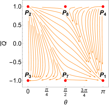
Figure 1: Orbits in the invariant set $(\theta,\bar{Q})$, with dynamics given by (156).

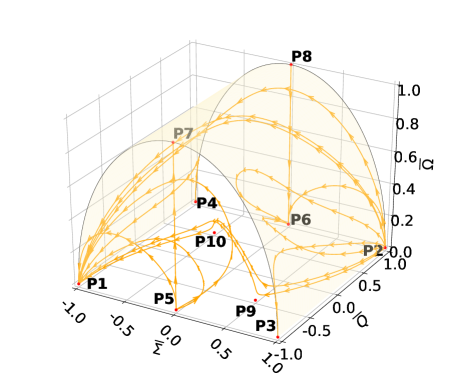
(a) Orbits in the phase space $(\bar{\Sigma},\bar{Q},\bar{\Omega})$.

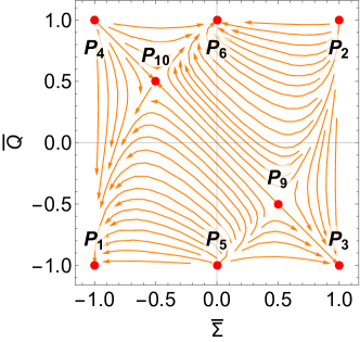
(b) Orbits in the invariant set $\bar{\Omega}=0$.

Figure 2: Phase space of the guiding system (139a), (139b), (139c) corresponding to KS for $\gamma=0$.

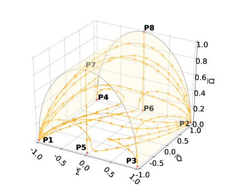
(a) Orbits in the phase space $(\bar{\Sigma},\bar{Q},\bar{\Omega})$.

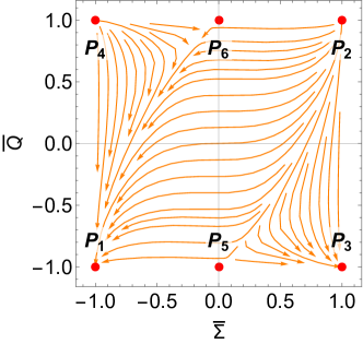
(b) Orbits in the invariant set $\bar{\Omega}=0$.

Figure 3: Phase space of the guiding system (139a), (139b), (139c) corresponding to KS for $\gamma=\frac{2}{3}$.

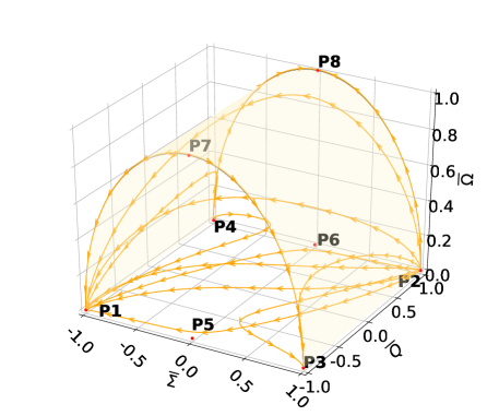
(a) Orbits in the phase space $(\bar{\Sigma},\bar{Q},\bar{\Omega})$.

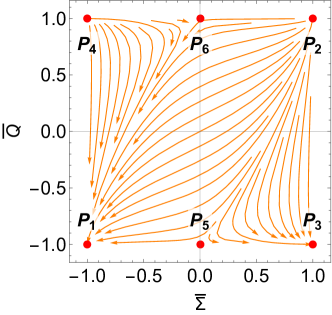
(b) Orbits in the invariant set $\bar{\Omega}=0$.

Figure 4: Phase space of the guiding system (139a), (139b), (139c) corresponding to KS for $\gamma=1$.

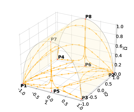
(a) Orbits in the phase space $(\bar{\Sigma},\bar{Q},\bar{\Omega})$.

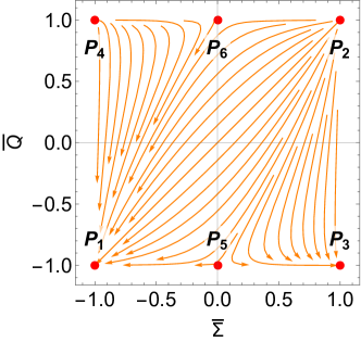
(b) Orbits in the invariant set $\bar{\Omega}=0$.

Figure 5: Phase space of the guiding system (139a), (139b), (139c) corresponding to KS for $\gamma=\frac{4}{3}$.

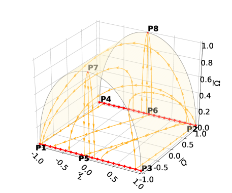
(a) Orbits in the phase space $(\bar{\Sigma},\bar{Q},\bar{\Omega})$.

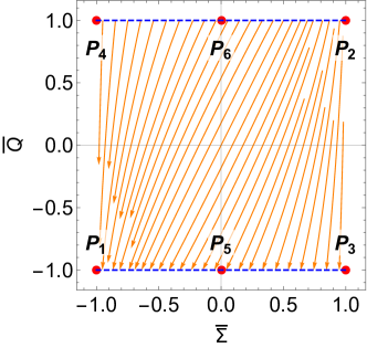
(b) Orbits in the invariant set $\bar{\Omega}=0$.

Figure 6: Phase space of the guiding system (139a), (139b), (139c) corresponding to KS for barotropic index $\gamma=2$.

In Figure 2 some orbits in the phase space of the guiding system (139a), (139b), (139c) for $\gamma=0$ corresponding to the CC are presented. In Figure 2(a) orbits in the phase space $(\bar{\Sigma},\bar{Q},\bar{\Omega})$ are displayed. In Figure 2(b) orbits in the invariant set $\bar{\Omega}=0$ are shown. Points $P_{2}$, $P_{4}$, and $P_{5}$ are early-time attractors. Points $P_{1},P_{3}$, and $P_{6}$ are late–time attractors. Points $P_{7}$, $P_{8}$, $P_{9}$, and $P_{10}$ are saddle points.

In Figure 3 some orbits of the phase space of the guiding system (139c) for $\gamma=\frac{2}{3}$ are presented. In Figure 3(a) some orbits in the phase space $(\bar{\Sigma},\bar{Q},\bar{\Omega})$ are displayed. In Figure 3(b) some orbits in the invariant set $\bar{\Omega}=0$ are shown. For the value of $\gamma=\frac{2}{3}$, $P_{5}$ coincides with $P_{9}$ and $P_{6}$ coincides with $P_{10}$. They are nonhyperbolic. Points $P_{2}$ and $P_{4}$ are early-time attractors. Points $P_{1}$ and $P_{3}$ are late–time attractors. Points $P_{5}$, $P_{6}$, $P_{7}$, and $P_{8}$ are saddle points.

In Figure 4 some orbits in the phase space of the guiding system (139a), (139b), (139c) for $\gamma=1$ which corresponds to dust are displayed. In Figure 4(a) some orbits in the phase space $(\bar{\Sigma},\bar{Q},\bar{\Omega})$ are presented. In Figure 4(b) some orbits in the invariant set $\bar{\Omega}=0$ are presented. Points $P_{2}$ and $P_{4}$ are early-time attractors. Points $P_{1}$ and $P_{3}$ are late–time attractors. Points $P_{5}$, $P_{6}$, $P_{7}$, and $P_{8}$ are saddle points.

In Figure 5 some orbits in the phase space of guiding system (139a), (139b), (139c) for $\gamma=\frac{4}{3}$ corresponding to radiation are presented. In Figure 5(a) some orbits in the phase space $(\bar{\Sigma},\bar{Q},\bar{\Omega})$ are displayed. In Figure 5(b) some orbits in the invariant set $\bar{\Omega}=0$ are shown. In both diagrams 5 and 6 points $P_{2}$ and $P_{4}$ are early-time attractors. Points $P_{1}$ and $P_{3}$ are late–time attractors. Points $P_{5},P_{6},P_{7}$, and $P_{8}$ are saddle points. Points $P_{9}$ and $P_{10}$ do not exist.

In Figure 6 some orbits in the phase space of guiding system (139a), (139b), (139c) for $\gamma=2$ which corresponds to stiff matter are presented. In Figure 6(a) some orbits in the phase space $(\bar{\Sigma},\bar{Q},\bar{\Omega})$ are displayed. In Figure 6(b) some orbits in the invariant set $\bar{\Omega}=0$ are shown. The line connecting points $P_{2},P_{4}$, and $P_{6}$ (denoted by a dashed blue line) is invariant, and it is the early-time attractor. The line connecting points $P_{1},P_{3}$, and $P_{5}$ (denoted by a dashed blue line) is invariant and it is the late–time attractor. Points $P_{7}$ and $P_{8}$ are saddle points. Points $P_{9}$ and $P_{10}$ do not exist.

5.1.1 late–time behavior in the reduce phase space

Now, we study the dynamics in the reduced phase space $\mathbf{x}=(\Omega,\Sigma,Q)$ where the effect of $D$ in the dynamics was neglected. The results from the linear stability analysis combined with Theorem 1 lead to the following local results.

Theorem 2

Late–time attractors of full system (89) and time–averaged system (139) as $D\rightarrow 0$ for Kantowski-Sachs line element are

1. The anisotropic solution $P_{1}$ with $\bar{\Omega}_{m}=0$ and line element (144) if $0\leq\gamma<2$. This point represents a non–flat LRS Kasner ($p_{1}=-\frac{1}{3},p_{2}=p_{3}=\frac{2}{3}$) contracting solution with $H<0$ (WE Sect. 6.2.2 and Sect. 9.1.1 (2)). This solution is singular at finite time $t_{0}=\frac{1}{3D_{0}}$ and is valid for $t>t_{0}$.

2. The anisotropic solution $P_{3}$ with $\bar{\Omega}_{m}=0$ and line element (145) if $0\leq\gamma<2$, representing a contracting solution with $H<0$. This point represents a Taub (flat LRS Kasner) contracting solution ($p_{1}=1,p_{2}=0,p_{3}=0$) WE (Sect 6.2.2 and p 193, eq. (9.6)).

3. The flat matter–dominated FLRW universe $P_{6}$ with metric (146) if $0<\gamma<\frac{2}{3}$. $P_{6}$ represents a quintessence fluid or a zero-acceleration (Dirac-Milne) model for $\gamma=\frac{2}{3}$. In the limit $\gamma=0$ we have
   $\ell(t)\propto\left(\frac{3\gamma D_{0}t}{2}+1\right)^{\frac{2}{3\gamma}}\rightarrow e^{D_{0}t}$, where $D_{0}=H_{0}$, i.e., the de Sitter solution.

For global results when $D\in[0,\infty)$ see section 6.

5.2 FLRW metric with positive curvature

In FLRW metric with positive curvature time–averaged system (135), (136), and (137) transforms to

$$\frac{d\bar{\Omega}}{d\eta}=\frac{3}{2}(\gamma-1)\bar{Q}\bar{\Omega}\left(1-{\bar{\Omega}}^{2}\right),$$ (157a)

$$\frac{d{\bar{Q}}}{d\eta}=-\frac{1}{2}\left(1-{\bar{Q}}^{2}\right)\left(3\gamma\left(1-{\bar{\Omega}}^{2}\right)+3{\bar{\Omega}}^{2}-2\right),$$ (157b)

$$\frac{d{\bar{\Phi}}}{d\eta}=0,$$ (157c)

$$\frac{d{D}}{d\eta}=-\frac{3}{2}\bar{Q}\left(\gamma(1-\bar{\Omega}^{2})+\bar{\Omega}^{2}\right)D.$$ (157d)

where $D$ is defined by eq. (87).

The equation for $\bar{\Omega}$ is simplified by setting $\bar{\Sigma}=0$ in eq. (140) and we define $\bar{\Omega}_{k}$ as $\bar{Q}^{2}\bar{\Omega}_{k}:=1-\bar{Q}^{2}$, where $\bar{\Omega}_{k}$ is interpreted as the time–averaged values of $\Omega_{k}:=\frac{1}{a^{2}H^{2}}$. Then, the phase space is

$$\left\{(\bar{\Omega},\bar{Q})\in\mathbb{R}^{2}:-1\leq\bar{Q}\leq 1,0\leq\bar{\Omega}\leq 1\right\}.$$ (158)

In some special cases we relax the condition $\bar{\Omega}\leq 1$ and consider $\bar{\Omega}>1$.

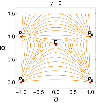
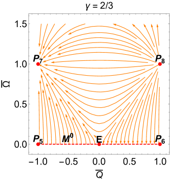
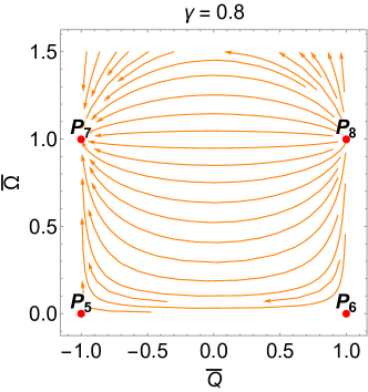
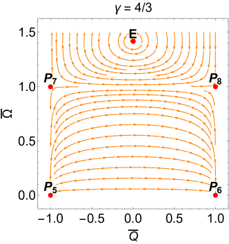
(a)

Figure 7: Phase plane for system (157a), (157b) corresponding to closed FLRW for different choices of $\gamma$.

Equilibrium points of (157a) and (157b) are

1. $P_{5}:(\bar{\Omega},\bar{Q})=(0,-1)$ with eigenvalues
   $\left\{2-3\gamma,-\frac{3}{2}(\gamma-1)\right\}$.

   1. It is a source for $0\leq\gamma<\frac{2}{3}$.

   2. It is a saddle for $\frac{2}{3}<\gamma<1$.

   3. It is nonhyperbolic for $\gamma=\frac{2}{3}$ and $\gamma=1$.

   4. It is a sink for $1<\gamma\leq 2$.

   This equilibrium point is related to the isotropic point $P_{5}$ of KS. The asymptotic metric at $P_{5}$ is given by

   $$ds^{2}=-dt^{2}+\frac{\left(1-\frac{3\gamma{D_{0}}t}{2}\right)^{\frac{4}{3\gamma}}}{{c_{1}}^{2}}dr^{2}$$

   $$+c_{1}\left(1-\frac{3\gamma D_{0}t}{2}\right)^{\frac{4}{3\gamma}}\sin^{2}r\;(d\vartheta^{2}+\sin^{2}\vartheta\,d\zeta^{2}).$$ (159)

   The corresponding solution is a flat matter–dominated FLRW contracting solution with $\bar{\Omega}_{m}=1$.

2. $P_{6}:(\bar{\Omega},\bar{Q})=(0,1)$ with eigenvalues
   $\left\{\frac{3}{2}(\gamma-1),3\gamma-2\right\}$.

   1. It is a sink for $0\leq\gamma<\frac{2}{3}$.

   2. It is a saddle for $\frac{2}{3}<\gamma<1$.

   3. It is nonhyperbolic for $\gamma=\frac{2}{3}$ and $\gamma=1$.

   4. It is a source for $1<\gamma\leq 2$.

   This equilibrium point is related to the isotropic point $P_{6}$ of KS. The asymptotic metric at the equilibrium point $P_{6}$ is

   $$ds^{2}=-dt^{2}+\frac{\left(\frac{3\gamma{D_{0}}t}{2}+1\right)^{\frac{4}{3\gamma}}}{{c_{1}}^{2}}dr^{2}$$

   $$+c_{1}\left(\frac{3\gamma D_{0}t}{2}+1\right)^{\frac{4}{3\gamma}}\sin^{2}r\;(d\vartheta^{2}+\sin^{2}\vartheta\,d\zeta^{2}).$$ (160)

   $P_{6}$ represents a quintessence fluid or a zero-acceleration (Dirac-Milne) model for $\gamma=\frac{2}{3}$. In the limit $\gamma=0$ we have $\ell(t)\propto\left(\frac{3\gamma D_{0}t}{2}+1\right)^{\frac{2}{3\gamma}}\rightarrow e^{D_{0}t}$, i.e., the de Sitter solution.

3. $P_{7}:(\bar{\Omega},\bar{Q})=(1,-1)$ with eigenvalues $\{-1,3(\gamma-1)\}$.

   1. It is a sink for $0\leq\gamma<1$.

   2. It is nonhyperbolic for $\gamma=1$.

   3. It is a saddle for $1<\gamma\leq 2$.

   This equilibrium point is related to the isotropic point $P_{7}$ of KS. The line element (71) becomes

   $$ds^{2}=-dt^{2}+c_{1}^{-2}{t^{\frac{4}{3}}}dr^{2}$$

   $$+{c_{2}^{-1}}{t^{\frac{4}{3}}}\sin^{2}r\;(d\vartheta^{2}+\sin^{2}\vartheta\,d\zeta^{2}).$$ (161)

   Hence, the equilibrium point can be associated with Einstein-de Sitter solution (WE , Sec 9.1.1 (1)) with $\gamma=1$. It is a contracting solution.

4. $P_{8}:(\bar{\Omega},\bar{Q})=(1,1)$ with eigenvalues $\{3-3\gamma,1\}$.

   1. It is a source for $0\leq\gamma<1$.

   2. It is nonhyperbolic for $\gamma=1$.

   3. It is a saddle for $1<\gamma\leq 2$.

   This equilibrium point is related to the isotropic point $P_{8}$ of KS. The line element (71) becomes

   $$ds^{2}=-dt^{2}+c_{1}^{-2}{t^{\frac{4}{3}}}dr^{2}$$

   $$+{c_{2}^{-1}}{t^{\frac{4}{3}}}\sin^{2}r\;(d\vartheta^{2}+\sin^{2}\vartheta\,d\zeta^{2}).$$ (162)

   Hence, the equilibrium point can be associated with Einstein-de Sitter solution (WE , Sec 9.1.1 (1)) with $\gamma=1$. It is an expanding solution.

5. $E:(\bar{\Omega},\bar{Q})=\left(\sqrt{\frac{3\gamma-2}{3\gamma-3}},0\right)$ with eigenvalues
   $\left\{-\frac{\sqrt{2-3\gamma}}{\sqrt{2}},\frac{\sqrt{2-3\gamma}}{\sqrt{2}}\right\}$. This point exists for $0\leq\gamma\leq\frac{2}{3}$ or $1<\gamma\leq 2$ and can be characterized as

   1. It is a saddle for $0\leq\gamma<\frac{2}{3}$.

   2. It is nonhyperbolic for $\gamma=\frac{2}{3}$ or $1<\gamma\leq 2$.

   This solution represents Einstein’s static universe. It is characterized by $k=1$, $\dot{\ell}=\ddot{\ell}=0$. It is usually viewed as a fluid model with a CC that is given a priori as a fixed universal constant Eddington:1930zz ; Harrison:1967zza ; Gibbons:1987jt ; Gibbons:1988bm ; Burd:1988ss ; Noh:2020vnk ; Barrow:2009sj ; Barrow:2003ni .

In the special case $\gamma=\frac{2}{3}$ there is one line of equilibrium points which are normally hyperbolic, $M^{0}:(\bar{\Omega},\bar{Q})=\left(0,\bar{Q}_{c}\right)$ with eigenvalues $\left\{-\frac{\bar{Q}_{c}}{2},0\right\}$, which is a sink for $\bar{Q}_{c}>0$ and a source for $\bar{Q}_{c}<0$.

The first equation of guiding system (135), (136), (137) becomes trivial up to second order in the $D$-expansion when $\gamma=1$. Using Taylor expansion up to the fourth order in $D$ the following time–averaged system is obtained

$$\frac{d\bar{\Omega}}{d\eta}=\frac{9D^{2}{\bar{Q}}\;\bar{\Omega}^{5}\left(\omega^{2}-2\mu^{2}\right)^{3}}{32b^{2}\mu^{6}\omega^{4}},$$ (163a)

$$\frac{d\bar{Q}}{d\eta}=-\frac{1}{32}\left(1-\bar{Q}^{2}\right)\left(\frac{9D^{2}\bar{\Omega}^{4}\left(\omega^{2}-2\mu^{2}\right)^{3}}{b^{2}\mu^{6}\omega^{4}}+16\right),$$ (163b)

$$\frac{d\bar{\Phi}}{d\eta}=\frac{3D\bar{\Omega}^{2}\left(\omega^{2}-2\mu^{2}\right)^{3}}{8b^{2}\mu^{6}\omega^{3}}-\frac{3D^{3}\bar{\Omega}^{4}\left(\omega^{2}-2\mu^{2}\right)^{5}}{32b^{4}\mu^{12}\omega^{5}},$$ (163c)

$$\frac{dD}{d\eta}=-\frac{3D{\bar{Q}}}{2}-\frac{9D^{3}{\bar{Q}}\;\bar{\Omega}^{4}\left(\omega^{2}-2\mu^{2}\right)^{3}}{32b^{2}\mu^{6}\omega^{4}}.$$ (163d)

Given

$$b\neq 0,\omega\neq 0,\mu\neq 0,{\omega^{2}-2\mu^{2}}\neq 0,{\bar{Q}}^{2}(\eta)\neq 1$$

$${-2{\bar{Q}}^{\prime}(\eta)+{\bar{Q}}^{2}(\eta)-1}\neq 0.$$ (164)

From eq. (163b) we have

$$\bar{\Omega}(\eta)=\frac{2\sqrt{b}\mu^{3/2}\omega\sqrt[4]{{\bar{Q}}(\eta)^{2}-2{\bar{Q}}^{\prime}(\eta)-1}}{\sqrt{3}\sqrt{D}\left(\omega^{2}-2\mu^{2}\right)^{3/4}\sqrt[4]{1-{\bar{Q}}^{2}(\eta)}}.$$ (165)

Substituting back eq. (165) in eq. (163) we have

$$D^{\prime}(\eta)=D(\eta){\bar{Q}}(\eta)\left(\frac{{\bar{Q}}^{\prime}(\eta)}{1-{\bar{Q}}^{2}(\eta)}-1\right).$$ (166)

Using the method of the integrating factor we define

$$v=e^{\int{\bar{Q}}(\eta)d\eta}D(\eta),$$ (167)

to obtain

$$v^{\prime}(\eta)= D^{\prime}(\eta)e^{\int{\bar{Q}}(\eta)\,d\eta}+D(\eta){\bar{Q}}(\eta)e^{\int{\bar{Q}}(\eta)\,d\eta}$$

$$= \frac{v(\eta){\bar{Q}}(\eta){\bar{Q}}^{\prime}(\eta)}{1-{\bar{Q}}^{2}(\eta)}\implies v(\eta)=\frac{v_{0}}{\sqrt{1-{\bar{Q}}^{2}(\eta)}}.$$ (168)

The integration constant can be absorbed in the indefinite integral. Then, we have

$$D(\eta)=\frac{e^{-\int{\bar{Q}}(\eta)\,d\eta}}{\sqrt{1-{\bar{Q}}^{2}(\eta)}}.$$ (169)

Substituting eq. (169) in eq. (165) we obtain

$$\bar{\Omega}(\eta)=\frac{2\sqrt{b}\mu^{3/2}\omega e^{\frac{1}{2}\int{\bar{Q}}(\eta)\,d\eta}}{\sqrt{3}\left(\omega^{2}-2\mu^{2}\right)^{3/4}}\sqrt[4]{{\bar{Q}}^{2}(\eta)-2{\bar{Q}}^{\prime}(\eta)-1}.$$ (170)

Then, substituting eqs. (169) and (170) in eq. (163c) we obtain the quadrature

$$\bar{\Phi}(\eta)=\frac{\left(\omega^{2}-2\mu^{2}\right)^{3/2}}{2b\mu^{3}\omega}\bigints\frac{\sqrt{{\bar{Q}}^{2}(\eta)-2{\bar{Q}}^{\prime}(\eta)-1}}{\sqrt{1-{\bar{Q}}^{2}(\eta)}}d\eta$$

$$-\frac{\left(\omega^{2}-2\mu^{2}\right)^{2}}{6b^{2}\mu^{6}\omega}\bigints\frac{D(\eta)\left({\bar{Q}}^{2}(\eta)-2{\bar{Q}}^{\prime}(\eta)-1\right)}{\left(1-{\bar{Q}}^{2}(\eta)\right)}d\eta.$$ (171)

Substituting eqs. (169), (170) in eq. (163a) we obtain under assumptions (164) the differential equation

$${\bar{Q}}^{\prime\prime}(\eta)={\bar{Q}(\eta)}\left(2({\bar{Q}(\eta)}^{2}-1)+{\bar{Q}}^{\prime}(\eta)\left(\frac{4{\bar{Q}}^{\prime}(\eta)}{{\bar{Q}(\eta)}^{2}-1}-5\right)\right).$$ (172)

Summarizing, system (163) admits the first integral (169), (170), (171), where ${\bar{Q}}$ satisfies the differential equation (172).

To analyze the asymptotic behavior of the solutions of eq. (172) we introduce the variables $x={\bar{Q}}(\eta),\;y={\bar{Q}}^{\prime}(\eta)$ to obtain

$$x^{\prime}(\eta)=y(\eta),$$ (173a)

$$y^{\prime}(\eta)=x(\eta)\left(2(x^{2}(\eta)-1)+y(\eta)\left(\frac{4y(\eta)}{x^{2}(\eta)-1}-5\right)\right).$$ (173b)

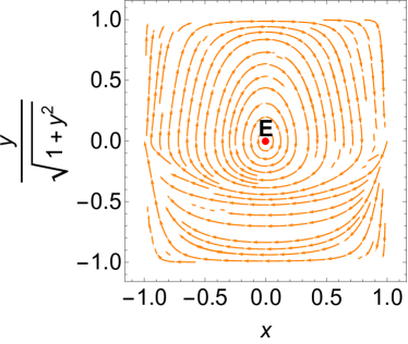
Figure 8: Compacted phase plane of system (173).

The origin is an equilibrium point with eigenvalues
$\left\{i\sqrt{2},-i\sqrt{2}\right\}$. The dynamics of system (173) in the coordinates $(x,y/\sqrt{1+y^{2}})$ is presented in Figure 8 where the origin is a stable center. According to the analysis at first order of the guiding system (135), (136), (137), Einstein’s static universe has coordinates $E:(\bar{\Omega},\bar{Q})=\left(\sqrt{\frac{3\gamma-2}{3\gamma-3}},0\right)$. When $\gamma=1$, this point satisfies $\bar{\Omega}\rightarrow\infty$. However, by taking $\gamma=1$ the equation for $\bar{\Omega}$ is decoupled and $\bar{\Omega}$ only takes arbitrary constant values. On the other hand, since $\gamma=1$, we required higher order terms in Taylor expansion for obtaining system (163). Since extra $\bar{\Omega}$- coordinate is excluded from Figure 8, Einstein’s static solution emerged. It is indeed a stable center in the $(Q,Q^{\prime})$ phase space. In Figure 8 the points $(x,y)=(-1,0)$ and $(x,y)=(1,0)$ are saddles.

Now, we study the dynamics in the reduced phase space $\mathbf{x}=(\Omega,Q)$, where the effect of $D$ in the dynamics was neglected. The results from the linear stability analysis combined with Theorem 1 for $\Sigma=0$ lead to the following local results.

Theorem 3

Late–time attractors of full system (125) and time–averaged system (157) as $D\rightarrow 0$ for closed FLRW metric with positive curvature line element are

1. The isotropic solution $P_{5}$ with metric (159) if $1<\gamma\leq 2$. The corresponding solution is a flat matter–dominated FLRW contracting solution with $\bar{\Omega}_{m}=1$.

2. The flat matter–dominated FLRW universe $P_{6}$ with metric (160) if $0<\gamma<\frac{2}{3}$. $P_{6}$ represents a quintessence fluid or a zero-acceleration (Dirac-Milne) model for $\gamma=\frac{2}{3}$. In the limit $\gamma=0$ we have
   $\ell(t)\propto\left(\frac{3\gamma D_{0}t}{2}+1\right)^{\frac{2}{3\gamma}}\rightarrow e^{D_{0}t}$, i.e., it corresponds to de Sitter solution.

3. The equilibrium point $P_{7}$ with metric (161) for $0\leq\gamma<1$. The equilibrium point can be associated with Einstein-de Sitter solution.

For global results when $D\in[0,\infty)$ see section 6.

6 Regular dynamical system on a compact phase space for Kantowski-Sachs and closed FLRW models

According to Remark 1, Theorem 1 is valid on a finite time scale where $D$, given by eq. (86), remains close to zero, but at a critical time $t^{*}$ we have $D^{\prime}(t^{*})=0$ and $D$ becomes strictly increasing when $t>t^{*}$ such that $\lim_{t\rightarrow\infty}D(t)=\infty.$ A lower bound for $t^{*}$ is estimated as $\bar{t}=\sup\{t>0:\Sigma(t)(1-Q^{2}(t)+3Q(t)\Sigma(t))>0\}$. If $\bar{t}=\infty$ this would mean that $\Sigma(t)(1-Q^{2}(t)+3Q(t)\Sigma(t))>0$ is invariant for the flow and $D\rightarrow 0$ as $t\rightarrow\infty,\eta\rightarrow\infty$, in contradiction to $\lim_{t\rightarrow\infty}D(t)=\infty$. Then, generically $\bar{t}<\infty$. A similar result follows for closed FLRW for $D$ defined by eq. (87) and taking $\Sigma=\Sigma_{0}=\bar{\Sigma}=0$.

These results are supported by the numerical evidence in B.1 and B.2.

6.1 Kantowski-Sachs metric

In this section we analyze qualitatively the time–averaged system (139) as $D\rightarrow\infty$ by introducing the variable

$$T=\frac{D}{1+D},$$ (174)

that maps $[0,\infty)$ to a finite interval $[0,1)$. Therefore, the limit $D\rightarrow+\infty$ corresponds to $T=1$ and the limit $D\rightarrow 0$ corresponds to $T=0$. Then, we have the guiding system (139a), (139b), (139c) extended with equation

$$\frac{dT}{d\eta}=\frac{1}{2}(1-T)T\left[3\bar{Q}\left((\gamma-2)\bar{\Sigma}^{2}+(\gamma-1)\bar{\Omega}^{2}-\gamma\right)+2\bar{Q}^{2}\bar{\Sigma}-2\bar{\Sigma}\right].$$ (175)

We are interested in late–time or early-time attractors, and in discussing relevant saddle equilibrium points of the extended dynamical system (139a), (139b), (139c) (175). In this regard, we have the following results.

1. $P_{1}:(\bar{\Omega},\bar{\Sigma},\bar{Q},T)=(0,-1,-1,0)$ with eigenvalues
   $\left\{-2,-\frac{3}{2},-3(2-\gamma),3\right\}$. It is saddle.

2. $P_{1}^{\infty}:(\bar{\Omega},\bar{\Sigma},\bar{Q},T)=(0,-1,-1,1)$ with eigenvalues
   $\left\{-2,-\frac{3}{2},-3(2-\gamma),-3\right\}$. It is a sink for $0\leq\gamma<2$.

3. $P_{2}:(\bar{\Omega},\bar{\Sigma},\bar{Q},T)=(0,1,1,0)$ with eigenvalues
   $\left\{2,\frac{3}{2},3(2-\gamma),-3\right\}$. It is saddle.

4. $P_{2}^{\infty}:(\bar{\Omega},\bar{\Sigma},\bar{Q},T)=(0,1,1,1)$ with eigenvalues
   $\left\{2,\frac{3}{2},3(2-\gamma),3\right\}$. It is a source for $0\leq\gamma<2$.

5. $P_{3}:(\bar{\Omega},\bar{\Sigma},\bar{Q},T)=(0,1,-1,0)$ with eigenvalues
   $\left\{-6,-\frac{3}{2},-3(2-\gamma),3\right\}$. It is saddle.

6. $P_{3}^{\infty}:(\bar{\Omega},\bar{\Sigma},\bar{Q},T)=(0,1,-1,1)$ with eigenvalues
   $\left\{-6,-\frac{3}{2},-3(2-\gamma),-3\right\}$. It is a sink for $0\leq\gamma<2$.

7. $P_{4}:(\bar{\Omega},\bar{\Sigma},\bar{Q},T)=(0,-1,1,0)$ with eigenvalues
   $\left\{6,\frac{3}{2},6-3\gamma,-3\right\}$. It is saddle.

8. $P_{4}^{\infty}:(\bar{\Omega},\bar{\Sigma},\bar{Q},T)=(0,-1,1,1)$ with eigenvalues
   $\left\{6,\frac{3}{2},6-3\gamma,3\right\}$. It is a source for $0\leq\gamma<2$.

9. $P_{5}:(\bar{\Omega},\bar{\Sigma},\bar{Q},T)=(0,0,-1,0)$ with eigenvalues
   $\left\{2-3\gamma,-\frac{3}{2}(\gamma-1),3-\frac{3\gamma}{2},\frac{3\gamma}{2}\right\}$. It is a source for $0<\gamma<\frac{2}{3}$.

10. $P_{5}^{\infty}:(\bar{\Omega},\bar{\Sigma},\bar{Q},T)=(0,0,-1,1)$ with eigenvalues
    $\left\{2-3\gamma,-\frac{3}{2}(\gamma-1),3-\frac{3\gamma}{2},-\frac{3\gamma}{2}\right\}$. It is a saddle.

11. $P_{6}:(\bar{\Omega},\bar{\Sigma},\bar{Q},T)=(0,0,1,0)$ with eigenvalues
    $\left\{\frac{3(\gamma-2)}{2},\frac{3(\gamma-1)}{2},3\gamma-2,-\frac{3\gamma}{2}\right\}$. It is a sink for $0<\gamma<\frac{2}{3}$.

12. $P_{6}^{\infty}:(\bar{\Omega},\bar{\Sigma},\bar{Q},T)=(0,0,1,1)$ with eigenvalues
    $\left\{\frac{3(\gamma-2)}{2},\frac{3(\gamma-1)}{2},3\gamma-2,\frac{3\gamma}{2}\right\}$. It is a saddle.

13. $P_{7}:(\bar{\Omega},\bar{\Sigma},\bar{Q},T)=(1,0,-1,0)$ with eigenvalues
    $\left\{-1,3(\gamma-1),\frac{3}{2},\frac{3}{2}\right\}$. It is saddle.

14. $P_{7}^{\infty}:(\bar{\Omega},\bar{\Sigma},\bar{Q},T)=(1,0,-1,1)$ with eigenvalues
    $\left\{-1,3(\gamma-1),\frac{3}{2},-\frac{3}{2}\right\}$. It is a saddle.

15. $P_{8}:(\bar{\Omega},\bar{\Sigma},\bar{Q},T)=(1,0,1,0)$ with eigenvalues
    $\left\{1,3(1-\gamma),-\frac{3}{2},-\frac{3}{2}\right\}$. It is saddle.

16. $P_{8}^{\infty}:(\bar{\Omega},\bar{\Sigma},\bar{Q},T)=(1,0,1,1)$ with eigenvalues
    $\left\{1,3(1-\gamma),-\frac{3}{2},\frac{3}{2}\right\}$. It is a saddle.

17. $P_{9}:(\bar{\Omega},\bar{\Sigma},\bar{Q},T)=\left(0,\frac{2-3\gamma}{\left|4-3\gamma\right|},-\frac{2}{\left|4-3\gamma\right|},0\right)$ with eigenvalues
    $\Bigg{\{}-\frac{3\left(\gamma+\sqrt{(2-\gamma)(\gamma(24\gamma-41)+18)}-2\right)}{2\left|4-3\gamma\right|},\frac{3\left(-\gamma+\sqrt{(2-\gamma)(\gamma(24\gamma-41)+18)}+2\right)}{2\left|4-3\gamma\right|}$,
    $\frac{3-3\gamma}{\left|4-3\gamma\right|},\frac{3\gamma}{\left|4-3\gamma\right|}\Bigg{\}}$ . Exists for $0\leq\gamma\leq\frac{2}{3}$ or $\gamma=2$ and is a saddle.

18. $P_{9}^{\infty}:(\bar{\Omega},\bar{\Sigma},\bar{Q},T)=\left(0,\frac{2-3\gamma}{\left|4-3\gamma\right|},-\frac{2}{\left|4-3\gamma\right|},1\right)$ with eigenvalues
    $\Bigg{\{}-\frac{3\left(\gamma+\sqrt{(2-\gamma)(\gamma(24\gamma-41)+18)}-2\right)}{2\left|4-3\gamma\right|},\frac{3\left(-\gamma+\sqrt{(2-\gamma)(\gamma(24\gamma-41)+18)}+2\right)}{2\left|4-3\gamma\right|}$,
    $\frac{3(1-\gamma)}{\left|4-3\gamma\right|},-\frac{3\gamma}{\left|4-3\gamma\right|}\Bigg{\}}$ . Exists for $0\leq\gamma\leq\frac{2}{3}$ or $\gamma=2$ and is a saddle.

19. $P_{10}:(\bar{\Omega},\bar{\Sigma},\bar{Q},T)=\left(0,\frac{3\gamma-2}{\left|4-3\gamma\right|},\frac{2}{\left|4-3\gamma\right|},0\right)$ with eigenvalues
    $\Bigg{\{}\frac{3\left(\gamma+\sqrt{(2-\gamma)(\gamma(24\gamma-41)+18)}-2\right)}{2\left|4-3\gamma\right|},-\frac{3\left(-\gamma+\sqrt{(2-\gamma)(\gamma(24\gamma-41)+18)}+2\right)}{2\left|4-3\gamma\right|}$,
    $-\frac{3(1-\gamma)}{\left|4-3\gamma\right|},-\frac{3\gamma}{\left|4-3\gamma\right|}\Bigg{\}}$. Exists for $0\leq\gamma\leq\frac{2}{3}$ or $\gamma=2$ and is saddle.

20. $P_{10}^{\infty}:(\bar{\Omega},\bar{\Sigma},\bar{Q},T)=\left(0,\frac{3\gamma-2}{\left|4-3\gamma\right|},\frac{2}{\left|4-3\gamma\right|},1\right)$ with eigenvalues
    $\Bigg{\{}\frac{3\left(\gamma+\sqrt{(2-\gamma)(\gamma(24\gamma-41)+18)}-2\right)}{2\left|4-3\gamma\right|},-\frac{3\left(-\gamma+\sqrt{(2-\gamma)(\gamma(24\gamma-41)+18)}+2\right)}{2\left|4-3\gamma\right|}$,
    $-\frac{3(1-\gamma)}{\left|4-3\gamma\right|},\frac{3\gamma}{\left|4-3\gamma\right|}\Bigg{\}}$. Exists for $0\leq\gamma\leq\frac{2}{3}$ or $\gamma=2$ and is saddle.

In the special case $\gamma=0$, there exist four lines of equilibrium points which are normally hyperbolic:

1. $I_{-}:(\bar{\Omega},\bar{\Sigma},\bar{Q},T)=\left(0,0,-1,T_{c}\right)$ with eigenvalues
   $\left\{3,2,\frac{3}{2},0\right\}$ is a source.

2. $I_{+}:(\bar{\Omega},\bar{\Sigma},\bar{Q},T)=\left(0,0,1,T_{c}\right)$ with eigenvalues
   $\left\{-3,-2,-\frac{3}{2},0\right\}$ is a sink.

3. $J_{-}:(\bar{\Omega},\bar{\Sigma},\bar{Q},T)=\left(0,\frac{1}{2},-\frac{1}{2},T_{c}\right)$ with eigenvalues $\left\{3,-\frac{3}{2},\frac{3}{4},0\right\}$ is a saddle.

4. $J_{+}:(\bar{\Omega},\bar{\Sigma},\bar{Q},T)=\left(0,-\frac{1}{2},\frac{1}{2},T_{c}\right)$ with eigenvalues $\left\{-3,\frac{3}{2},-\frac{3}{4},0\right\}$ is a saddle.

In the special case $\gamma=1$ there exist four lines of equilibrium points which are normally hyperbolic, say,

1. $K_{-}:(\bar{\Omega},\bar{\Sigma},\bar{Q},T)=(\bar{\Omega}_{c},0,-1,0)$ with eigenvalues $\left\{\frac{3}{2},\frac{3}{2},-1,0\right\}$ is a saddle.

2. $K_{+}:(\bar{\Omega},\bar{\Sigma},\bar{Q},T)=(\bar{\Omega}_{c},0,1,0)$ with eigenvalues
   $\left\{-\frac{3}{2},-\frac{3}{2},1,0\right\}$ is a saddle.

3. $K_{-}^{\infty}:(\bar{\Omega},\bar{\Sigma},\bar{Q},T)=(\bar{\Omega}_{c},0,-1,1)$ with eigenvalues
   $\left\{-\frac{3}{2},\frac{3}{2},-1,0\right\}$ is a saddle.

4. $K_{+}^{\infty}:(\bar{\Omega},\bar{\Sigma},\bar{Q},T)=(\bar{\Omega}_{c},0,1,1)$ with eigenvalues
   $\left\{-\frac{3}{2},\frac{3}{2},1,0\right\}$ is a saddle.

In the special case $\gamma=2$ there exist four lines of equilibrium points which are normally hyperbolic, say,

1. $L_{-}:(\bar{\Omega},\bar{\Sigma},\bar{Q},T)=(0,\bar{\Sigma}_{c},-1,0)$ with eigenvalues
   $\left\{3,-\frac{3}{2},0,-2\bar{\Sigma}_{c}-4\right\}$ is a saddle.

2. $L_{+}:(\bar{\Omega},\bar{\Sigma},\bar{Q},T)=(0,\bar{\Sigma}_{c},1,0)$ with eigenvalues
   $\left\{-3,\frac{3}{2},0,4-2\bar{\Sigma}_{c}\right\}$ is a saddle.

3. $L_{-}^{\infty}:(\bar{\Omega},\bar{\Sigma},\bar{Q},T)=(0,\bar{\Sigma}_{c},-1,1)$ with eigenvalues
   $\left\{-3,-\frac{3}{2},0,-2\bar{\Sigma}_{c}-4\right\}$ is a sink for $\bar{\Sigma}_{c}>-2$.

4. $L_{+}^{\infty}:(\bar{\Omega},\bar{\Sigma},\bar{Q},T)=(0,\bar{\Sigma}_{c},1,1)$ with eigenvalues
   $\left\{3,\frac{3}{2},0,4-2\bar{\Sigma}_{c}\right\}$ is a source for $\bar{\Sigma}_{c}<2$.

As before, the subindex $\pm$ indicates if they correspond to contracting (“$-$”) or to expanding (“$+$”) solutions. Superindex $\infty$ refers to solutions with $D\rightarrow\infty$.

For KS model the extended phase is four dimensional. To illustrate the stability of the aforementioned normally hyperbolic lines we examine numerically some invariant sets. In Figure 9 the dynamics at the invariant set $\bar{\Omega}=0$ corresponding to vacuum solutions is represented in the compact space $(\bar{\Sigma},D/(1+D),\bar{Q})$ for $\gamma=0$ and $\gamma=2$.

For $\gamma=1$ and $\bar{\Sigma}=0$, the model is reduced to the closed FLRW metric with dust. The stability of the lines $K_{\pm}$ and $K_{\pm}^{\infty}$ on this invariant set corresponding to isotropic solutions is illustrated in Figure 10(c).

Also, we refer to Figures 13, 14, 15, 16, 17, 18, 19, and 20, where projections of some orbits of the full system and the averaged system are presented. In these figures it is numerically confirmed the result of Theorem 1 for KS metric. That is to say, solutions of the full system (blue lines) follow the track of the solutions of the averaged system (orange lines) for the whole $D$-range.

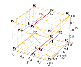
(a) Cosmological constant $\gamma=0$.

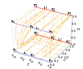
(b) Stiff matter $\gamma=2$.

Figure 9: Dynamics of the averaged system (139) at the invariant set $\bar{\Omega}=0$ for $\gamma=0$ and $2$, represented in the compact space $(\bar{\Sigma},D/(1+D),\bar{Q})$.

6.2 FLRW metric with positive curvature

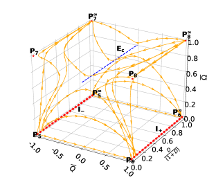
(a) Cosmological constant $\gamma=0$.

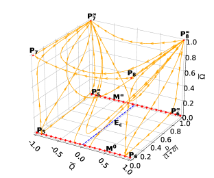
(b) Zero acceleration $\gamma=\frac{2}{3}$.

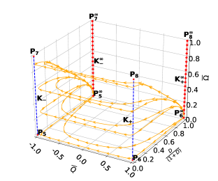
(c) Dust $\gamma=1$.

Figure 10: Dynamics of the averaged system (157) for $\gamma=0$ and $\frac{2}{3}$, and of the averaged system (163) for $\gamma=1$, represented in the compact space  $(\bar{Q},D/(1+D),\bar{\Omega})$.

Using the variable (174) the time–averaged system for $\gamma\neq 1$ (157) becomes the guiding system (157a) and (157b) extended with equation

$$\frac{dT}{d\eta}=\frac{3}{2}(1-T)T\bar{Q}\left[(\gamma-1)\bar{\Omega}^{2}-\gamma\right].$$ (176)

We are interested in late–time or early-time attractors and in discussing the relevant saddle equilibrium points of the extended system (157a), (157b) and (176). In this regard, we have the following results.

1. $P_{5}:(\bar{\Omega},\bar{Q},T)=(0,-1,0)$ with eigenvalues
   $\left\{2-3\gamma,-\frac{3}{2}(\gamma-1),\frac{3\gamma}{2}\right\}$ is a source for $0<\gamma<\frac{2}{3}$.

2. $P_{5}^{\infty}:(\bar{\Omega},\bar{Q},T)=(0,-1,1)$ with eigenvalues
   $\left\{2-3\gamma,-\frac{3}{2}(\gamma-1),-\frac{3\gamma}{2}\right\}$ is a sink for $1<\gamma\leq 2$.

3. $P_{6}:(\bar{\Omega},\bar{Q},T)=(0,1,0)$ with eigenvalues
   $\left\{\frac{3(\gamma-1)}{2},3\gamma-2,-\frac{3\gamma}{2}\right\}$ is a sink $0<\gamma<\frac{2}{3}$.

4. $P_{6}^{\infty}:(\bar{\Omega},\bar{Q},T)=(0,1,1)$ with eigenvalues
   $\left\{\frac{3(\gamma-1)}{2},3\gamma-2,\frac{3\gamma}{2}\right\}$ is a source for $1<\gamma\leq 2$.

5. $P_{7}:(\bar{\Omega},\bar{Q},T)=(1,-1,0)$ with eigenvalues
   $\left\{-1,3(\gamma-1),\frac{3}{2}\right\}$. It is saddle.

6. $P_{7}^{\infty}:(\bar{\Omega},\bar{Q},T)=(1,-1,1)$ with eigenvalues
   $\left\{-1,3(\gamma-1),-\frac{3}{2}\right\}$ is a sink for $0\leq\gamma<1$.

7. $P_{8}:(\bar{\Omega},\bar{Q},T)=(1,1,0)$ with eigenvalues
   $\left\{3-3\gamma,1,-\frac{3}{2}\right\}$ is a source for $0\leq\gamma<1$. It is saddle.

8. $P_{8}^{\infty}:(\bar{\Omega},\bar{Q},T)=(1,1,1)$ with eigenvalues
   $\left\{3-3\gamma,1,\frac{3}{2}\right\}$ is a source for $0\leq\gamma<1$.

9. $E_{c}:(\bar{\Omega},\bar{Q},T)=\left(\sqrt{\frac{{3\gamma-2}}{{3\gamma-3}}},0,T_{c}\right)$ with eigenvalues
   $\left\{0,-\sqrt{\frac{(5-3\gamma)\gamma-2}{2(\gamma-1)}},\sqrt{\frac{(5-3\gamma)\gamma-2}{2(\gamma-1)}}\right\}$. This line of equilibrium points exists for $0\leq\gamma\leq\frac{2}{3}$ or $1<\gamma\leq 2$ and can be characterized as a nonhyperbolic saddle for $0\leq\gamma<\frac{2}{3}$. For $1<\gamma\leq 2$ two eigenvalues are purely imaginary and one eigenvalue is zero. Then, it can be a center or a focus.

In the special case $\gamma=0$ there exist two lines of equilibrium points which are normally hyperbolic, say,

1. $I_{-}:(\bar{\Omega},\bar{Q},T)=\left(0,-1,T_{c}\right)$ with eigenvalues
   $\left\{2,\frac{3}{2},0\right\}$ is a source.

2. $I_{+}:(\bar{\Omega},\bar{Q},T)=\left(0,1,T_{c}\right)$ with eigenvalues
   $\left\{-2,-\frac{3}{2},0\right\}$ is a sink.

In the special case $\gamma=\frac{2}{3}$ there exists two lines of equilibrium points which are normally hyperbolic, say,

1. $M^{0}:(\bar{\Omega},\bar{Q},T)=\left(0,\bar{Q}_{c},0\right)$ with eigenvalues
   $\left\{-\bar{Q}_{c},-\frac{\bar{Q}_{c}}{2},0\right\}$ is a sink for $\bar{Q}_{c}>0$ and a source for $\bar{Q}_{c}<0$.

2. $M^{\infty}:(\bar{\Omega},\bar{Q},T)=\left(0,\bar{Q}_{c},1\right)$ with eigenvalues
   $\left\{\bar{Q}_{c},-\frac{\bar{Q}_{c}}{2},0\right\}$ is a saddle.

In the special case $\gamma=1$ there exist four lines of equilibrium points which are normally hyperbolic, say,

1. $K_{-}:(\bar{\Omega},\bar{Q},T)=(\bar{\Omega}_{c},-1,0)$ with eigenvalues
   $\left\{\frac{3}{2},-1,0\right\}$ is a saddle.

2. $K_{+}:(\bar{\Omega},\bar{Q},T)=(\bar{\Omega}_{c},1,0)$ with eigenvalues
   $\left\{-\frac{3}{2},1,0\right\}$ is a saddle.

3. $K_{-}^{\infty}:(\bar{\Omega},\bar{Q},T)=(\bar{\Omega}_{c},-1,1)$ with eigenvalues
   $\left\{-\frac{3}{2},-1,0\right\}$ is a sink.

4. $K_{+}^{\infty}:(\bar{\Omega},\bar{Q},T)=(\bar{\Omega}_{c},1,1)$ with eigenvalues
   $\left\{\frac{3}{2},1,0\right\}$ is a source.

In Figure 10 the dynamics of the averaged system (157) for $\gamma=0$, $\frac{2}{3}$ and of the averaged system (163) for $\gamma=1$ is represented in the compact space  $(\bar{Q},D/(1+D),\bar{\Omega})$. In Figures 13, 14, 15, 16, 17, 18, 19, and 20 projections of some solutions of the full system (89) and time–averaged system (139) in the $(\Sigma,D/(1+D),\Omega^{2})$ and $(Q,D,\Omega^{2})$ space are presented with their respective projections when $D=0$. In figures 21, 22, 23, and 24 projections of some solutions of the full system (125) and time–averaged system (157) for $\gamma\neq 1$ and of system (163) for $\gamma=1$ in the $(Q,D/(1+D),\Omega^{2})$ space are presented with their respective projection when $D=0$. Figures 21 and 25 show how the solutions of the full system (blue lines) follow the track of the solutions of the averaged system (orange lines) for the whole $D$-range. Figures 22, 23, 24, and 26 are evidence that the main theorem presented in Section 4 is fulfilled for the FLRW metric with positive curvature ($k=+1$) only when $D$ is bounded. Precisely, the solutions of the full system (blue lines) follow the track of the solutions of the averaged system (orange lines) for the time interval $tD=\mathcal{O}(1)$. However, when $D$ becomes infinite ($T\rightarrow 1$) and for $\gamma\geq 1$ we have the following conjecture. For closed Friedmann–Lemaître-Robertson–Walker (FLRW) and $1\leq\gamma\leq 2$ the solutions of the full system depart from the solutions of the averaged system.

6.2.1 Closed FLRW: regime $\Omega>1$

Now, we describe the regime $\Omega>1$. We define

$$U(\phi)=2f^{2}\left(1-\cos\left(\frac{\phi}{f}\right)\right)-{\phi^{2}}.$$ (177)

Substituting the form of potential (14) in constraint (85e) we obtain for closed FLRW models

$$3D^{2}:=3H^{2}+\frac{3}{\ell^{2}}= \rho_{m}+\frac{1}{2}\dot{\phi}^{2}+\frac{\omega^{2}}{2}\phi^{2}+\frac{\left(\omega^{2}-2\mu^{2}\right)}{2}U(\phi).$$ (178)

Then,

$$1=\frac{\rho_{m}}{3D^{2}}+\frac{\dot{\phi}^{2}}{6D^{2}}+\frac{\omega^{2}\phi^{2}}{6D^{2}}+\frac{\left(\omega^{2}-2\mu^{2}\right)}{6D^{2}}U(\phi).$$ (179)

Using definition (87) we obtain

$$1=\frac{\rho_{m}}{3D^{2}}+\Omega^{2}+\frac{\left(\omega^{2}-2\mu^{2}\right)}{6D^{2}}U(\phi).$$ (180)

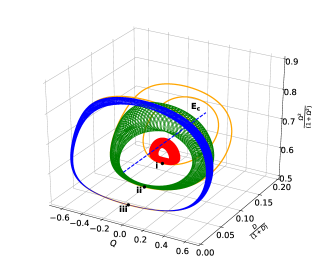
(a) Projections in the space $(Q,D/(1+D),\Omega^{2}/(1+\Omega^{2}))$.

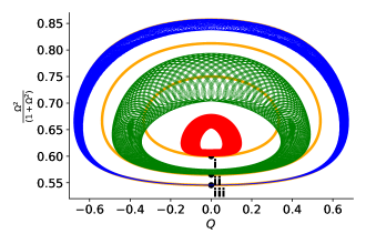
(b) Projection in the space $(Q,\Omega^{2}/(1+\Omega^{2}))$.

Figure 11: Some solutions of the full system (125) (blue) and time–averaged system (157) (orange) for the FLRW metric with positive curvature ($k=+1$) when $\gamma=\frac{4}{3}$. We have used for both systems the initial data sets presented in Table 2.

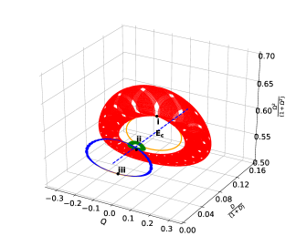
(a) Projections in the space $(Q,D/(1+D),\Omega^{2}/(1+\Omega^{2}))$.

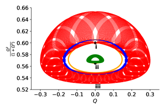
(b) Projection in the space $(Q,\Omega^{2}/(1+\Omega^{2}))$.

Figure 12: Some solutions of the full system (125) (blue) and time–averaged system (157) (orange) for the FLRW metric with positive curvature ($k=+1$) when $\gamma=2$. We have used for both systems the initial data sets presented in Table 2.

Table 2: Here we present three initial data sets for the simulation of full system (125) and time–averaged system (157) for FLRW metric with positive curvature ($k=+1$) and for $\gamma=\frac{4}{3}$ (radiation) and $\gamma=2$ (stiff fluid). All the conditions are chosen in order to fulfill the inequalities $\Omega>1$ and $0\leq Q\leq 1$.

Sol.	$D(0)$	$\Omega^{2}(0)$	$Q(0)$	$\varphi(0)$	$t(0)$
i	$0.1$	$1.5$	$0$	$0$	$0$
ii	$0.05$	$1.3$	$0$	$0$	$0$
iii	$0.01$	$1.2$	$0$	$0$	$0$

The function $U(\phi)$ defined by eq. (177) satisfies $U^{\prime}(0)=U^{\prime\prime}(0)=U^{\prime\prime\prime}(0)=0$, and $U^{(iv)}(0)=-\frac{2}{f^{2}}$, which implies that $\phi=0$ is a global degenerated maximum of order 2 for $U(\phi)$. Therefore, $U(\phi)\leq 0$. Then, from $\omega^{2}>2\mu^{2}$ and (180) it follows that $\Omega$, $\Sigma^{2}$ and $\frac{\rho_{m}}{3D^{2}}$ can be greater than 1. This implies that we can have solutions with $\Omega>1$ preserving the non-negativity of the energy densities. That is, even if $U(\phi)\leq 0$, we have $\frac{\omega^{2}}{2}\phi^{2}+\frac{\left(\omega^{2}-2\mu^{2}\right)}{2}U(\phi)\geq 0$ because the sign of term $\frac{\omega^{2}}{2}\phi^{2}$ is dominant over the last term in eq. (180).

This interesting behavior when $\Omega>1$ can be seen in Figures 7(a), 8, 11 and 12, where we show the solutions of the full system (125) and the time–averaged system (157) considering the values $\gamma=\frac{4}{3}$ and $\gamma=2$ and using as initial conditions the three data sets presented in Table 2.

This dynamical behavior related to spiral tubes has been presented before in the literature in Heinzle:2004sr and it is related to the fact that the line of equilibrium points $E_{c}$ (representing Einstein’s static universes) has purely imaginary eigenvalues. In Heinzle:2004sr a comprehensive dynamical description for closed cosmologies when the matter source admits Einstein’s static model was presented. Moreover, theorems about the global asymptotic behavior of solutions were established. Results in Heinzle:2004sr and Heinzle:2006zy disprove claims of non-predictability and chaos for models close to Einstein’s model given in deOliveira:1997ej ; Barguine:2001rb ; DeOliveira:2002ih ; Soares:2005fn .

To illustrate the existence of spiral tubes we integrate the full system (125) and the time–averaged system (157) using the fixed constants $\mu=\sqrt{2}/2$, $b=\sqrt{2}/5$, $\omega=\sqrt{2}$, $f=\frac{b\mu^{3}}{\omega^{2}-2\mu^{2}}=1/10\geq 0$. We select $\gamma=\frac{4}{3}$ and $\gamma=2$ for the barotropic index (cases where $E_{c}$ exists), and we use as initial conditions the three data sets presented in Table 2. In Figures 11 and 12 projections of the orbits showing this behavior in the $(Q,D/(1+D),\Omega^{2})$ space are presented with their respective projection when $D=0$. Figures 11(a) and 11(b) show solutions for a fluid corresponding to radiation ($\gamma=\frac{4}{3}$). Figures 12(a) and 12(b) show solutions for a fluid corresponding to stiff fluid ($\gamma=2$).

7 Conclusions

This is the last paper of the “Averaging generalized scalar field cosmologies” research program. We have used asymptotic methods and averaging theory to explore the solutions space of scalar field cosmologies with generalized harmonic potential (13) in vacuum or minimally coupled to matter. Different from references Leon:2021lct ; Leon:2021rcx , here we have studied systems where Hubble scalar is not monotonic, but the systems admit a function $D$ given by eq. (12) playing the role of a time-depending perturbation parameter, which is decreasing for a finite time scale $t<t^{*}$ where $D^{\prime}(t^{*})=0$. For $t>t^{*}$ monotony of the quantity $D$ changes and this parameter increases without bound.

We have proved Theorem 1 which states that late–time attractors of full and time–averaged systems are the same when the quantity $D$ tends to zero. More specifically, according to Theorem 1 for KS metrics and positively curved FLRW models, the quantity $D$ controls the magnitude of error between full time–dependent and time–averaged solutions as $D\rightarrow 0$. Therefore, the analysis of the system is reduced to study the corresponding time–averaged equation as $D\rightarrow 0$. However, for KS metric the initial region $0<Q<1,\Sigma^{2}+\Omega^{2}<1,\Sigma(1-Q^{2}+3Q\Sigma)>0$ (and for closed FLRW the initial region $Q>0$, respectively) is not invariant for the full system (89) and for the time–averaged equations (102), (103), (104), (105), and (106). According to Remark 1, Theorem 1 is valid on a time scale $t<t^{*}$ where $D$ remains close to zero, but $D(t)$ changes its monotony at a critical time $t^{*}$ becoming monotonic increasing without bound.

We have formulated Theorems 2 and 3 concerning the late–time behavior of our model valid when the evolution equation for $D$ is decoupled, whose proofs are based on Theorem 1 and linear stability analysis. Hence, we can establish the stability of a periodic solution as it exactly matches the stability of the stationary solution of the time–averaged equation. In particular, for KS metric the local late–time attractor of full system (89) and time–averaged system (139) (where the evolution equation for $D$ is decoupled) are the following.

1. The anisotropic solution $P_{1}$ with $\bar{\Omega}_{m}=0$ if $0\leq\gamma<2$, which represents a non–flat LRS Kasner ($p_{1}=-\frac{1}{3},p_{2}=p_{3}=\frac{2}{3}$) contracting solution with $H<0$. This solution is singular at finite time $t_{1}=\frac{1}{3D_{0}}$ and is valid for $t>t_{1}$.

2. The anisotropic solution $P_{3}$ with $\bar{\Omega}_{m}=0$ if $0\leq\gamma<2$, which represents a Taub (flat LRS Kasner) contracting solution ($p_{1}=1,p_{2}=0,p_{3}=0$) WE .

3. The flat matter–dominated FLRW universe $P_{6}$ if $0\leq\gamma<\frac{2}{3}$. $P_{6}$ represents a quintessence fluid or a zero-acceleration (Dirac-Milne) model for $\gamma=\frac{2}{3}$. In the limit $\gamma=0$ we have the de Sitter solution.

We have commented that, although for $t<t^{*}$, $D(t)$ remains close to zero, once the orbit crosses the initial region, $D$ changes its monotony, and it becomes strictly increasing without bound. Hence, Theorem 1 is valid on a time scale $tD=\mathcal{O}(1)$. To investigate the region $D\rightarrow\infty$ we have used the transformation of coordinates (174) that maps $[0,\infty)$ to a finite interval $[0,1)$. Therefore, the limit $D\rightarrow+\infty$ corresponds to $T=1$ and the limit $D\rightarrow 0$ corresponds to $T=0$. This defines a regular dynamical system over a compact phase space that allows to obtain global results. We have studied the stability of the fixed points in a compactified phase space. These numerical results support the claim that late–time attractors in the extended phase space $(\mathbf{x},T)$, where $T=\frac{D}{1+D}$ and $\mathbf{x}=(\Omega,\Sigma,Q)$ for both the original system and the time–averaged are the same for KS. When the stability of the equilibrium point of the time–averaged is analyzed in extended phase space, we find for KS metric that the extra variable $T$ introduces equilibrium points “at infinity”, $P_{1}^{\infty}$ which is a non–flat LRS Kasner solution and $P_{3}^{\infty}$ which is Taub (flat LRS Kasner). They are contracting solutions and sink for $0\leq\gamma<2$ in the extended (global) phase space. Their analogous points $P_{1}$ and $P_{3}$ (with $D=H=T=0$) become saddle along the $T$-axis in the extended phase space. The only equilibrium point that remains a sink for KS for $0\leq\gamma<\frac{2}{3}$ in the extended phase space is $P_{6}$.

Figures 13, 14, 15, 16, 17, 18, 19, and 20 are a numerical confirmation that main Theorem 1 presented in Section 4 is fulfilled for the KS metric. That is to say, the solutions of the full system (blue lines) follow the track of the solutions of the averaged system (orange lines) for the whole $D$-range.

On the other hand, local late–time attractors of full system (125) and time–averaged system (157) (where the evolution equation for $D$ is decoupled) for closed FLRW metric with positive curvature are the following.

1. The isotropic solution $P_{5}$ if $1<\gamma\leq 2$. The corresponding solution is a flat matter–dominated FLRW contracting solution with $\bar{\Omega}_{m}=1$.

2. The flat matter–dominated FLRW universe $P_{6}$ if $0\leq\gamma<\frac{2}{3}$. $P_{6}$ represents a quintessence fluid or a zero-acceleration (Dirac-Milne) model for $\gamma=\frac{2}{3}$. In the limit $\gamma=0$ we have the de Sitter solution.

3. The equilibrium point $P_{7}$ if $0\leq\gamma<1$. The equilibrium point can be associated with Einstein-de Sitter solution.

When the stability of the equilibrium point of the time–averaged extended phase space for closed FLRW metric is analyzed in the extended phase space $(\mathbf{x},T)$, where $\mathbf{x}=(\Omega,Q)$, for closed FLRW we find that the extra variable $T$ introduces equilibrium points “at infinity”, $P_{5}^{\infty}$ which is a sink for $1<\gamma\leq 2$ and $P_{7}^{\infty}$ which is a sink for $0\leq\gamma<1$. As for KS, the only equilibrium point that remains a sink for KS for $0\leq\gamma<\frac{2}{3}$ in the extended phase space is $P_{6}$.

In Figures 21, 22, 23, and 24 we have presented projections of some solutions of the full system (125) and time–averaged system (157) for $\gamma\neq 1$. Also, system (163) for $\gamma=1$ in the $(Q,D/(1+D),\Omega^{2})$ space are presented with its respective projection when $D=0$. Figures 21 and 25 show how solutions of the full system (blue lines) follow the track of solutions of the averaged system (orange lines) for the whole $D$-range. Figures 22, 23, 24, and 26 are evidence that main theorem presented in Section 4 is fulfilled for FLRW metric with positive curvature ($k=+1$) only when $D$ is bounded. Namely, the solutions of the full system (blue lines) follow the track of solutions of the averaged system (orange lines) for the time interval $tD=\mathcal{O}(1)$. However, when $D$ becomes infinite ($T\rightarrow 1$) and for $\gamma\geq 1$, the solutions of full system (blue lines) depart from solutions of averaged system (orange lines) as $D$ becomes large. Then, different from KS, for the full system and given $\gamma\geq 1$ the orbits (blue lines) do not follow the track of solutions of the averaged system, while $P_{8}^{\infty}$ and $P_{7}^{\infty}$ are early and late–time attractor, respectively, as $D\rightarrow\infty$. This is a rather different behavior from time–averaged system, where they are saddle. This can be anticipated because when $D$ becomes large, the approximation obtained under the assumption of small $D$ fails.

Additionally, for closed FLRW we have found by numerical tools the existence of spiral tubes confined in a finite region of the phase space when the line of equilibrium points $E_{c}$ (representing Einstein’s static universes) exist. This kind of dynamical structures have been presented before in reference Heinzle:2004sr and they exist for any matter source that admits Einstein’s static model. Results in the line of Heinzle:2004sr are of interest since they disprove the claims of non-predictability and chaos for models close to Einstein’s model related to the existence of infinitely many homoclinic orbits whose $\alpha$ and $\omega$- limits are the same periodic orbit producing chaotic sets in the whole state space. Thus, a set of models in a neighborhood of Einstein’s model were claimed to be unpredictable and characterized by “homoclinic chaos” deOliveira:1997ej ; Barguine:2001rb ; DeOliveira:2002ih ; Soares:2005fn . However, the asserted “homoclinic phenomena”, if they occur at all, must be confined to narrow regions of the phase space Heinzle:2004sr (see also Heinzle:2006zy ).

Now, we summarize the results of the “Averaging generalized scalar field cosmologies” research program. In reference Leon:2021lct it was proved that for LRS Bianchi III the late–time attractors are a matter–dominated flat FLRW universe if $0\leq\gamma\leq\frac{2}{3}$ (mimicking de Sitter, quintessence or zero acceleration solutions), a matter–curvature scaling solution if $\frac{2}{3}<\gamma<1$, and Bianchi III flat spacetime for $1\leq\gamma\leq 2$. For FLRW metric with $k=-1$ the late–time attractors are flat matter–dominated FLRW universe if $0\leq\gamma\leq\frac{2}{3}$ and Milne solution if $\frac{2}{3}<\gamma<2$. In all metrics, matter–dominated flat FLRW universe represents quintessence fluid if $0<\gamma<\frac{2}{3}$. In reference Leon:2021rcx for flat FLRW and LRS Bianchi I metrics it was obtained that late–time attractors of full and time–averaged systems are given by flat matter–dominated FLRW solution and Einstein-de Sitter solution. It is interesting to note that for FLRW with negative or zero curvature and for Bianchi I metric when the matter fluid corresponds to a CC, $H$ asymptotically tends to constant values depending on initial conditions. That is consistent with de Sitter expansion. In addition, for FLRW models with negative curvature for any $\gamma<\frac{2}{3}$ and $\Omega_{k}>0$, $\Omega_{k}\rightarrow 0$, or when $\gamma>\frac{2}{3}$ and $\Omega_{k}>0$ the universe becomes curvature dominated ($\Omega_{k}\rightarrow 1$). For flat FLRW and dust background from the qualitative analysis performed in paper Leon:2021rcx we have that $\lim_{\tau\rightarrow+\infty}\bar{\Omega}(\tau)=\text{const.}$, and $\lim_{\tau\rightarrow+\infty}H(\tau)=0$. Also, it was numerically proved that as $H\rightarrow 0$, the values of $\bar{\Omega}$ give an upper bound for the values $\Omega$ of the original system. Therefore, by controlling the error of the time–averaged higher order system the error of the original system can also be controlled.

Finally, in the present research we have proved that in KS metric the global late–time attractors of full and time–averaged systems are two anisotropic contracting solutions, $P_{1}^{\infty}$ which is a non–flat LRS Kasner and $P_{3}^{\infty}$ which is a Taub (flat LRS Kasner) for $0\leq\gamma<2$, and $P_{6}$ which is a matter–dominated flat FLRW universe if $0\leq\gamma\leq\frac{2}{3}$ (mimicking de Sitter, quintessence or zero acceleration solutions). For FLRW metric with $k=+1$ global late–time attractors of time–averaged system are $P_{5}^{\infty}$ which is a flat matter–dominated contracting solution that is a sink for $1<\gamma\leq 2$, $P_{6}$ which is a matter–dominated flat FLRW universe mimicking de Sitter, quintessence or zero acceleration solutions if $0\leq\gamma\leq\frac{2}{3}$, and the point $P_{7}^{\infty}$ which is an Einstein-de Sitter solution for $0\leq\gamma<1$ and large $t$. However, when $D$ becomes infinite ($T\rightarrow 1$) and for $\gamma\geq 1$ solutions of the full system (blue lines) depart from solutions of averaged system (orange lines) as $D$ is large. Then, different from KS, for the full system and given $\gamma>1$ the orbits (blue lines) do not follow the track of the averaged system and $P_{8}^{\infty}$ and $P_{7}^{\infty}$ are the early and late–time attractor, respectively, as $D\rightarrow\infty$. This is a rather different behavior from the time–averaged system, where they are saddle. Therefore, this analysis completes the characterization of the full class of homogeneous but anisotropic solutions and their isotropic limits with exception of LRS Bianchi V. Our analytical results were strongly supported by numerical results in B. We have shown that asymptotic methods and averaging theory are powerful tools to investigate scalar field cosmologies with generalized harmonic potential.

Appendix A Proof of Theorem 1

Lemma 4 (Gronwall’s Lemma (Integral form))

Let $\xi(t)$ be a nonnegative function summable over $[0,T]$, which satisfies almost everywhere the integral inequality

$$\xi(t)\leq C_{1}\int_{0}^{t}\xi(s)ds+C_{2},\;C_{1},C_{2}\geq 0.$$

Then, $\xi(t)\leq C_{2}e^{C_{1}t},$ almost everywhere for $t$ in $0\leq t\leq T$. In particular, if

$$\xi(t)\leq C_{1}\int_{0}^{t}\xi(s)ds,\;C_{1}\geq 0,$$

almost everywhere for $t$ in $0\leq t\leq T$. Then, $\xi\equiv 0$ almost everywhere for $t$ in $0\leq t\leq T$.

Lemma 5 (Mean value Theorem)

Let $U\subset\mathbb{R}^{n}$ be open, $\mathbf{f}:U\rightarrow\mathbb{R}^{m}$ continuously differentiable, and $\mathbf{x}\in U$, $\mathbf{h}\in\mathbb{R}^{m}$ vectors such that the line segment $\mathbf{x}+z\;\mathbf{h}$, $0\leq z\leq 1$ remains in $U$. Then, we have

$$\mathbf{f}(\mathbf{x}+\mathbf{h})-\mathbf{f}(\mathbf{x})=\left(\int_{0}^{1}\mathbb{D}\mathbf{f}(\mathbf{x}+z\;\mathbf{h})\,dz\right)\cdot\mathbf{h},$$ (181)

where $\mathbb{D}\mathbf{f}$ denotes the Jacobian matrix of $\mathbf{f}$ and the integral of a matrix is understood as a componentwise.

A.1 Proof of Theorem 1.

From eq. (93) $D$ is a monotonic decreasing function of $t$ whenever $0<Q<1,\Sigma^{2}+\Omega^{2}<1,\Sigma(1-Q^{2}+3Q\Sigma)>0$. The last restriction holds, in particular, by choosing $Q>0,\Sigma>0$. In the last case we define the bootstrapping sequences

$$\left\{\begin{array}[]{c}t_{0}=t_{0},\\ \\ D_{0}=D(t_{0})\end{array}\right.,$$ (185)

$$\left\{\begin{array}[]{c}{t_{n+1}}={t_{n}}+\frac{1}{D_{n}}\\ \\ D_{n+1}=D(t_{n+1})\end{array}\right..$$ (189)

This sequence, however, is finite; that is, $t_{n}<t^{*}$ with $t^{*}$ such that $\lim_{t\rightarrow t^{*}}D^{\prime}(t)=0.$ If $Q(t_{n})<0$ or $\Sigma(t_{n})<0$ for some $n$ we stop the integration because $D$ changes its monotony to become a monotonic increasing function. However, $(t,\eta,\Sigma,Q,\Phi)\mapsto(-t,-\eta,-\Sigma,-Q,-\Phi)$ leaves invariant the system. Therefore, the solution is completed by using the above symmetry.

Given expansions (107), system (117) becomes

$$\dot{\Omega_{0}}= \frac{1}{2}D{Q_{0}}{\Omega_{0}}\Bigg{(}3\gamma\left(1-{\Sigma_{0}}^{2}-{\Omega_{0}}^{2}\right)-2{Q_{0}}{\Sigma_{0}}+6{\Sigma_{0}}^{2}+3{\Omega_{0}}^{2}-3\Bigg{)}$$

$$+\frac{3}{2}D{Q_{0}}\left({\Omega_{0}}^{2}-1\right){\Omega_{0}}\cos(2({\Phi_{0}}-t\omega))$$

$$+D{\Sigma_{0}}{\Omega_{0}}-D\frac{\partial g_{1}}{\partial t}+\mathcal{O}(D^{2}),$$ (190)

$$\dot{\Sigma_{0}}= \frac{1}{2}D\Bigg{(}\left({\Sigma_{0}}^{2}-1\right)\left(-2{Q_{0}}^{2}-3(\gamma-2){Q_{0}}{\Sigma_{0}}+2\right)-3(\gamma-1){Q_{0}}{\Sigma_{0}}{\Omega_{0}}^{2}\Bigg{)}$$

$$+\frac{3}{2}D{Q_{0}}{\Sigma_{0}}{\Omega_{0}}^{2}\cos(2({\Phi_{0}}-t\omega))-D\frac{\partial g_{2}}{\partial t}+\mathcal{O}(D^{2}),$$ (191)

$$\dot{Q_{0}}= \frac{1}{2}D\left(1-{Q_{0}}^{2}\right)\Bigg{(}3\gamma\left({\Sigma_{0}}^{2}+{\Omega_{0}}^{2}-1\right)+2{\Sigma_{0}}({Q_{0}}-3{\Sigma_{0}})-3{\Omega_{0}}^{2}+2\Bigg{)}$$

$$+\frac{3}{2}D\left({Q_{0}}^{2}-1\right){\Omega_{0}}^{2}\cos(2({\Phi_{0}}-t\omega))-D\frac{\partial g_{3}}{\partial t}+\mathcal{O}(D^{2}),$$ (192)

$$\dot{\Phi_{0}}= \left(\frac{3}{2}{Q_{0}}\sin(2({\Phi_{0}}-t\omega))-\frac{\partial g_{4}}{\partial t}\right)D+\mathcal{O}\left(D^{2}\right).$$ (193)

Let $\Delta\mathbf{x}_{0}(t)=(\Omega_{0}-\bar{\Omega},{\Sigma_{0}}-\bar{\Sigma},{Q_{0}}-\bar{Q})^{T}$ and $\Delta\Phi_{0}=\Phi_{0}-\bar{\Phi}$. Taking the initial conditions $\Omega_{0}(t_{n})=\bar{\Omega}(t_{n})={\Omega_{n}},\;\Sigma_{0}(t_{n})=\bar{\Sigma}(t_{n})={\Sigma}_{n},$ $Q_{0}(t_{n})=\bar{Q}(t_{n})={Q}_{n},\;\Phi_{0}(t_{n})=\bar{\Phi}(t_{n})={\Phi}_{n},$ such that

$$0<Q_{n}<1,\Sigma_{n}^{2}+\Omega_{n}^{2}<1,\Sigma_{n}(1-Q_{n}^{2}+3Q_{n}\Sigma_{n})>0,$$

Eqs. (123) become

$$\frac{\partial g_{1}}{\partial t}=\frac{3}{2}{Q_{0}}{\Omega_{0}}\left({\Omega_{0}}^{2}-1\right)\cos(2({\Phi_{0}}-t\omega)),$$ (194a)

$$\frac{\partial g_{2}}{\partial t}=\frac{3}{2}{Q_{0}}{\Sigma_{0}}{\Omega_{0}}^{2}\cos(2({\Phi_{0}}-t\omega)),$$ (194b)

$$\frac{\partial g_{3}}{\partial t}=\frac{3}{2}\left({Q_{0}}^{2}-1\right){\Omega_{0}}^{2}\cos(2({\Phi_{0}}-t\omega)),$$ (194c)

$$\frac{\partial g_{4}}{\partial t}=\frac{3}{2}{Q_{0}}\sin(2({\Phi_{0}}-t\omega)),$$ (194d)

Explicit expressions for $g_{i}$ obtained by integration of (194) are given by

$$g_{1}(D,\Omega_{0},\Sigma_{0},Q_{0},\Phi_{0},t)=\frac{3}{4\omega}{Q_{0}}{\Omega_{0}}\left(1-{\Omega_{0}}^{2}\right)\sin(2({\Phi_{0}}-t\omega)),$$ (195)

$$g_{2}(D,\Omega_{0},\Sigma_{0},Q_{0},\Phi_{0},t)=-\frac{3}{4\omega}{Q_{0}}{\Sigma_{0}}{\Omega_{0}}^{2}\sin(2({\Phi_{0}}-t\omega)),$$ (196)

$$g_{3}(D,\Omega_{0},\Sigma_{0},Q_{0},\Phi_{0},t)=\frac{3}{4\omega}\left(1-{Q_{0}}^{2}\right){\Omega_{0}}^{2}\sin(2({\Phi_{0}}-t\omega)),$$ (197)

$$g_{4}(D,\Omega_{0},\Sigma_{0},Q_{0},\Phi_{0},t)=\frac{3Q_{0}\cos(2(\Phi_{0}-t\omega))}{4\omega},$$ (198)

where we have set four integration functions
$C_{i}(D,\Omega_{0},\Sigma_{0},Q_{0},\Phi_{0}),i=1,2,3,4$ to zero. The functions $g_{i},i=1,2,3,4$ are continuously differentiable such that their partial derivatives are bounded on $t\in[t_{n},t_{n+1}]$.

The second order expansion around $D=0$ of system (122) is written as  

$$\dot{\Delta\Omega_{0}}=\frac{1}{2}D\Bigg{(}\bar{\Omega}\left(3\bar{Q}\left((\gamma-2)\bar{\Sigma}^{2}+(\gamma-1)\left(\bar{\Omega}^{2}-1\right)\right)+2\bar{Q}^{2}\bar{\Sigma}-2\bar{\Sigma}\right)+\Omega_{0}\left(Q_{0}\left(-3\gamma\left(\Sigma_{0}^{2}+\Omega_{0}^{2}-1\right)-2Q_{0}\Sigma_{0}+6\Sigma_{0}^{2}+3\Omega_{0}^{2}-3\right)+2\Sigma_{0}\right)\Bigg{)}$$

$$+D^{2}\sin(2(\Phi_{0}-t\omega))\Bigg{(}\frac{\Omega_{0}\cos(2(\Phi_{0}-t\omega))\left(-9b^{2}\mu^{6}\omega^{2}\left(\Omega_{0}^{2}-1\right)\left(\left(5Q_{0}^{2}-1\right)\Omega_{0}^{2}+Q_{0}^{2}\right)-2\Omega_{0}^{2}\left(2\mu^{2}-\omega^{2}\right)^{3}\right)}{8b^{2}\mu^{6}\omega^{3}}+\frac{\Omega_{0}^{3}\left(2\mu^{2}-\omega^{2}\right)^{3}}{4b^{2}\mu^{6}\omega^{3}}$$

$$+\frac{3\Omega_{0}\left(-3\gamma\Sigma_{0}^{2}+3\gamma+\Omega_{0}^{2}\left(-3\gamma+Q_{0}\left(2\left(Q_{0}^{2}-1\right)\Sigma_{0}+3(\gamma-2)Q_{0}\Sigma_{0}^{2}-3\gamma Q_{0}+Q_{0}\right)+2\right)+3(\gamma-1)Q_{0}^{2}\Omega_{0}^{4}+2Q_{0}^{2}+6\Sigma_{0}^{2}-2\right)}{8\omega}\Bigg{)},$$ (199)

$$\dot{\Delta\Sigma_{0}}=\frac{1}{2}D\left(\left(\bar{Q}^{2}-1\right)\left(3(\gamma-2)\bar{\Sigma}^{2}+3(\gamma-1)\bar{\Omega}^{2}+2\bar{Q}\bar{\Sigma}-3\gamma+2\right)+\left(\Sigma_{0}^{2}-1\right)\left(-2Q_{0}^{2}-3(\gamma-2)Q_{0}\Sigma_{0}+2\right)-3(\gamma-1)Q_{0}\Sigma_{0}\Omega_{0}^{2}\right)$$

$$+D^{2}\sin(2(\Phi_{0}-t\omega))\Bigg{(}\frac{3\Omega_{0}^{2}\left(Q_{0}\left(2Q_{0}^{2}\left(\Sigma_{0}^{2}-1\right)+Q_{0}\Sigma_{0}\left(3\gamma\left(\Sigma_{0}^{2}+\Omega_{0}^{2}-1\right)-6\Sigma_{0}^{2}-3\Omega_{0}^{2}+4\right)-2\Sigma_{0}^{2}+2\right)-4\Sigma_{0}\right)}{8\omega}$$

$$\quad\quad\quad\quad\quad\quad\quad\quad\quad\quad+\frac{9\left(1-5Q_{0}^{2}\right)\Sigma_{0}\Omega_{0}^{4}\cos(2(\Phi_{0}-t\omega))}{8\omega}\Bigg{)},$$ (200)

$$\dot{\Delta Q_{0}}=\frac{1}{2}D\left(3(\gamma-1)\bar{Q}\bar{\Sigma}\bar{\Omega}^{2}-\left(\bar{\Sigma}^{2}-1\right)\left(-3(\gamma-2)\bar{Q}\bar{\Sigma}-2\bar{Q}^{2}+2\right)+\left(1-Q_{0}^{2}\right)\left(3\gamma\left(\Sigma_{0}^{2}+\Omega_{0}^{2}-1\right)+2\Sigma_{0}(Q_{0}-3\Sigma_{0})-3\Omega_{0}^{2}+2\right)\right)$$

$$+D^{2}\sin(2(\Phi_{0}-t\omega))\left(\frac{3Q_{0}\left(Q_{0}^{2}-1\right)\Omega_{0}^{2}\left(3\gamma\left(\Sigma_{0}^{2}+\Omega_{0}^{2}-1\right)+2\Sigma_{0}(Q_{0}-3\Sigma_{0})-3\Omega_{0}^{2}\right)}{8\omega}-\frac{45Q_{0}\left(Q_{0}^{2}-1\right)\Omega_{0}^{4}\cos(2(\Phi_{0}-t\omega))}{8\omega}\right),$$ (201)

$$\dot{\Delta\Phi_{0}}=D^{2}\Bigg{(}\frac{3\bar{\Omega}^{2}\left(2\mu^{2}-\omega^{2}\right)^{3}}{8b^{2}\mu^{6}\omega^{3}}+\frac{\cos(2(\Phi_{0}-t\omega))\left(3b^{2}\mu^{6}\omega^{2}\left(-3\gamma\left(\Sigma_{0}^{2}+\Omega_{0}^{2}-1\right)+2Q_{0}^{2}+6\Sigma_{0}^{2}+3\Omega_{0}^{2}-2\right)+4\Omega_{0}^{2}\left(2\mu^{2}-\omega^{2}\right)^{3}\right)}{8b^{2}\mu^{6}\omega^{3}}$$

$$+\frac{9b^{2}\mu^{6}\omega^{2}\left(2Q_{0}^{2}+\Omega_{0}^{2}\right)+\cos(4(\Phi_{0}-t\omega))\left(9b^{2}\mu^{6}\omega^{2}\left(2Q_{0}^{2}\left(\Omega_{0}^{2}+1\right)-\Omega_{0}^{2}\right)-2\Omega_{0}^{2}\left(2\mu^{2}-\omega^{2}\right)^{3}\right)-6\Omega_{0}^{2}\left(2\mu^{2}-\omega^{2}\right)^{3}}{16b^{2}\mu^{6}\omega^{3}}\Bigg{)}.$$ (202)

Denoting $\mathbf{x}_{0}=(\Omega_{0},\Sigma_{0},Q_{0})^{T}$, $\bar{\mathbf{x}}=(\bar{\Omega},\bar{\Sigma},\bar{Q})^{T}$, and $\Delta\mathbf{x}_{0}(t)=(\Omega_{0}-\bar{\Omega},{\Sigma_{0}}-\bar{\Sigma},{Q_{0}}-\bar{Q})^{T}$ with $0\leq|\Delta\mathbf{x}_{0}|:=\max\left\{|\Omega_{0}-\bar{\Omega}|,|{\Sigma_{0}}-\bar{\Sigma}|,|{Q_{0}}-\bar{Q}|\right\}<\infty$ in the closed interval $[t_{n},t]$, Eqs. (122) are reduced to a 3-dimensional system

$$\dot{\Delta\mathbf{x}_{0}}=D\left(\bar{\mathbf{f}}({\mathbf{x}}_{0})-\bar{\mathbf{f}}(\bar{\mathbf{x}})\right)+\mathcal{O}(D^{2}),$$ (203)

plus eq. (202), where the vector function $\bar{\mathbf{f}}$ in eq. (122) is explicitly given by

$$\bar{\mathbf{f}}(y_{1},y_{2},y_{3})=\left(\begin{array}[]{c}-\frac{1}{2}y_{1}\left(3(\gamma-1)\left(y_{1}^{2}-1\right)y_{3}+3(\gamma-2)y_{2}^{2}y_{3}+2y_{2}\left(y_{3}^{2}-1\right)\right)\\ \frac{1}{2}\left(\left(y_{2}^{2}-1\right)\left(-3(\gamma-2)y_{2}y_{3}-2y_{3}^{2}+2\right)-3(\gamma-1)y_{1}^{2}y_{2}y_{3}\right)\\ -\frac{1}{2}\left(y_{3}^{2}-1\right)\left(-3\gamma+3(\gamma-1)y_{1}^{2}+3(\gamma-2)y_{2}^{2}+2y_{2}y_{3}+2\right)\\ \end{array}\right).$$

The last row corresponding to $\dot{\Delta\Phi_{0}}$ was omitted. This vector function with polynomial components in variables $(y_{1},y_{2},y_{3})$ is continuously differentiable in all its components.

Using the same initial conditions for $\mathbf{x}_{0}$ and $\bar{\mathbf{x}}$, we obtain by integration

$$\Delta\mathbf{x}_{0}(t)=\int_{t_{n}}^{t}\dot{\Delta\mathbf{x}_{0}}ds=\int_{t_{n}}^{t}\left(D\left(\bar{\mathbf{f}}({\mathbf{x}}_{0})-\bar{\mathbf{f}}(\bar{\mathbf{x}})\right)+\mathcal{O}(D^{2})\right)ds.$$ (204)

The terms of order $\mathcal{O}(D^{2})$ under the integral sign in eq. (204) come from the second order terms in the series expansion centered in $D=0$ of $\dot{\Delta}\Omega_{0}$, $\dot{\Delta}\Sigma_{0}$, and $\dot{\Delta}Q_{0}$ in eqs. (199), (200), and (201). These terms are bounded in the interval $[t_{n},t_{n+1}]$ by $M_{1}D_{n}^{2}$, where

$$M_{1}=\max_{t\in[t_{n},t_{n+1}]}\Bigg{\{}\Bigg{|}\frac{\Omega_{0}\cos(2(\Phi_{0}-t\omega))\left(-9b^{2}\mu^{6}\omega^{2}\left(\Omega_{0}^{2}-1\right)\left(\left(5Q_{0}^{2}-1\right)\Omega_{0}^{2}+Q_{0}^{2}\right)-2\Omega_{0}^{2}\left(2\mu^{2}-\omega^{2}\right)^{3}\right)}{8b^{2}\mu^{6}\omega^{3}}+\frac{\Omega_{0}^{3}\left(2\mu^{2}-\omega^{2}\right)^{3}}{4b^{2}\mu^{6}\omega^{3}}$$

$$+\frac{3\Omega_{0}\left(-3\gamma\Sigma_{0}^{2}+3\gamma+\Omega_{0}^{2}\left(-3\gamma+Q_{0}\left(2\left(Q_{0}^{2}-1\right)\Sigma_{0}+3(\gamma-2)Q_{0}\Sigma_{0}^{2}-3\gamma Q_{0}+Q_{0}\right)+2\right)+3(\gamma-1)Q_{0}^{2}\Omega_{0}^{4}+2Q_{0}^{2}+6\Sigma_{0}^{2}-2\right)}{8\omega}\Bigg{|},$$

$$\Bigg{|}\frac{3\Omega_{0}^{2}\left(Q_{0}\left(2Q_{0}^{2}\left(\Sigma_{0}^{2}-1\right)+Q_{0}\Sigma_{0}\left(3\gamma\left(\Sigma_{0}^{2}+\Omega_{0}^{2}-1\right)-6\Sigma_{0}^{2}-3\Omega_{0}^{2}+4\right)-2\Sigma_{0}^{2}+2\right)-4\Sigma_{0}\right)}{8\omega}+\frac{9\left(1-5Q_{0}^{2}\right)\Sigma_{0}\Omega_{0}^{4}\cos(2(\Phi_{0}-t\omega))}{8\omega}\Bigg{|},$$

$$\Bigg{|}\frac{3Q_{0}\left(Q_{0}^{2}-1\right)\Omega_{0}^{2}\left(3\gamma\left(\Sigma_{0}^{2}+\Omega_{0}^{2}-1\right)+2\Sigma_{0}(Q_{0}-3\Sigma_{0})-3\Omega_{0}^{2}\right)}{8\omega}-\frac{45Q_{0}\left(Q_{0}^{2}-1\right)\Omega_{0}^{4}\cos(2(\Phi_{0}-t\omega))}{8\omega}\Bigg{|}\Bigg{\}},$$

is finite by continuity of $\bar{\Omega},\Omega_{0},\bar{\Sigma},\Sigma_{0},\bar{Q},Q_{0},\Phi_{0}$ in the interval $[t_{n},t_{n+1}]$. Taking the sup norm $|\Delta\mathbf{x}_{0}|=\max\left\{|\Omega_{0}-\bar{\Omega}|,|{\Sigma_{0}}-\bar{\Sigma}|,|{Q_{0}}-\bar{Q}|\right\}$ we have

$$\Big{|}\Delta\mathbf{x}_{0}(t)\Big{|}=\Big{|}\int_{t_{n}}^{t}\dot{\Delta\mathbf{x}_{0}}ds\Big{|}=\Bigg{|}\int_{t_{n}}^{t}\Bigg{(}D\left(\bar{\mathbf{f}}({\mathbf{x}}_{0})-\bar{\mathbf{f}}(\bar{\mathbf{x}})\right)+\mathcal{O}(D^{2})\Bigg{)}ds\Bigg{|}$$

$$\leq D_{n}\int_{t_{n}}^{t}\Big{|}\bar{\mathbf{f}}({\mathbf{x}}_{0})-\bar{\mathbf{f}}(\bar{\mathbf{x}})\Big{|}ds+M_{1}D_{n}^{2}(t-t_{n}),$$

for all $t\in[t_{n},t_{n+1}]$.
Using Lemma 5 we have

$$\bar{\mathbf{f}}({\mathbf{x}}_{0}(s))-\bar{\mathbf{f}}(\bar{\mathbf{x}}(s))={\mathbb{A}(s)}\cdot\left({\mathbf{x}}_{0}(s)-\bar{\mathbf{x}}(s)\right),$$ (205)

where

$$\mathbb{A}(s)=\left(\int_{0}^{1}\mathbb{D}\bar{\mathbf{f}}\left(\bar{\mathbf{x}}(s)+\tau\left({\mathbf{x}}_{0}(s)-\bar{\mathbf{x}}(s)\right)\right)\,d\tau\right),$$ (206)

$\mathbb{D}\bar{\mathbf{f}}$ denotes the Jacobian matrix of $\bar{\mathbf{f}}$ and the integral of a matrix is understood as a componentwise. We denote the matrix elements of $\mathbb{A}$ as

$$\mathbb{A}(s)=\left(\begin{array}[]{ccc}a_{11}(s)&a_{12}(s)&a_{13}(s)\\ a_{21}(s)&a_{22}(s)&a_{23}(s)\\ a_{31}(s)&a_{32}(s)&a_{33}(s)\\ \end{array}\right),$$ (207)

where $a_{ij}$ are polynomial functions of $\bar{\Omega},\Omega_{0},\bar{\Sigma},\Sigma_{0},\bar{Q},Q_{0}$, and they are explicitly given by

$$a_{11}(s)= \frac{1}{24}\bar{Q}\left(-6(\gamma-2)\Sigma_{0}\bar{\Sigma}-9(\gamma-2)\bar{\Sigma}^{2}-9(\gamma-1)\left(2\Omega_{0}\bar{\Omega}+3\bar{\Omega}^{2}+\Omega_{0}^{2}-2\right)-3(\gamma-2)\Sigma_{0}^{2}\right)$$

$$+Q_{0}\left(\frac{1}{24}\left(-6(\gamma-2)\Sigma_{0}\bar{\Sigma}-3(\gamma-2)\bar{\Sigma}^{2}-9(\gamma-1)\left(2\Omega_{0}\bar{\Omega}+\bar{\Omega}^{2}+3\Omega_{0}^{2}-2\right)-9(\gamma-2)\Sigma_{0}^{2}\right)+\frac{1}{6}\bar{Q}\left(-\bar{\Sigma}-\Sigma_{0}\right)\right)$$

$$+\frac{1}{12}\bar{Q}^{2}\left(-3\bar{\Sigma}-\Sigma_{0}\right)+\frac{1}{12}Q_{0}^{2}\left(-\bar{\Sigma}-3\Sigma_{0}\right)+\frac{1}{2}\left(\bar{\Sigma}+\Sigma_{0}\right),$$ (208a)

$$a_{12}(s)= -\frac{1}{4}(\gamma-2)\bar{Q}\left(\bar{\Sigma}\left(3\bar{\Omega}+\Omega_{0}\right)+\Sigma_{0}\left(\bar{\Omega}+\Omega_{0}\right)\right)+Q_{0}\left(\frac{1}{6}\bar{Q}\left(-\bar{\Omega}-\Omega_{0}\right)-\frac{1}{4}(\gamma-2)\left(\bar{\Sigma}\left(\bar{\Omega}+\Omega_{0}\right)+\Sigma_{0}\left(\bar{\Omega}+3\Omega_{0}\right)\right)\right)$$

$$+\frac{1}{12}\bar{Q}^{2}\left(-3\bar{\Omega}-\Omega_{0}\right)+\frac{1}{12}Q_{0}^{2}\left(-\bar{\Omega}-3\Omega_{0}\right)+\frac{1}{2}\left(\bar{\Omega}+\Omega_{0}\right),$$ (208b)

$$a_{13}(s)= \frac{1}{8}\Bigg{(}-2(\gamma-2)\Sigma_{0}\bar{\Sigma}\left(\bar{\Omega}+\Omega_{0}\right)-(\gamma-2)\bar{\Sigma}^{2}\left(3\bar{\Omega}+\Omega_{0}\right)+\bar{\Omega}\left(-3(\gamma-1)\bar{\Omega}\left(\bar{\Omega}+\Omega_{0}\right)-\gamma\left(\Sigma_{0}^{2}+3\Omega_{0}^{2}-6\right)+2\Sigma_{0}^{2}+3\Omega_{0}^{2}-6\right)$$

$$+3\Omega_{0}\left(-\gamma\left(\Sigma_{0}^{2}+\Omega_{0}^{2}-2\right)+2\Sigma_{0}^{2}+\Omega_{0}^{2}-2\right)\Bigg{)}+\frac{1}{6}\bar{Q}\left(-\bar{\Sigma}\left(3\bar{\Omega}+\Omega_{0}\right)-\Sigma_{0}\left(\bar{\Omega}+\Omega_{0}\right)\right)$$

$$+\frac{1}{6}Q_{0}\left(-\bar{\Sigma}\left(\bar{\Omega}+\Omega_{0}\right)-\Sigma_{0}\left(\bar{\Omega}+3\Omega_{0}\right)\right),$$ (208c)

$$a_{21}(s)= -\frac{1}{4}(\gamma-1)\bar{Q}\left(\bar{\Sigma}\left(3\bar{\Omega}+\Omega_{0}\right)+\Sigma_{0}\left(\bar{\Omega}+\Omega_{0}\right)\right)-\frac{1}{4}(\gamma-1)Q_{0}\left(\bar{\Sigma}\left(\bar{\Omega}+\Omega_{0}\right)+\Sigma_{0}\left(\bar{\Omega}+3\Omega_{0}\right)\right),$$ (208d)

$$a_{22}(s)= \frac{1}{8}\bar{Q}\left(-6(\gamma-2)\Sigma_{0}\bar{\Sigma}-9(\gamma-2)\bar{\Sigma}^{2}-(\gamma-1)\bar{\Omega}\left(3\bar{\Omega}+2\Omega_{0}\right)-3(\gamma-2)\left(\Sigma_{0}^{2}-2\right)-(\gamma-1)\Omega_{0}^{2}\right)$$

$$+Q_{0}\left(\frac{1}{8}\left(-6(\gamma-2)\Sigma_{0}\bar{\Sigma}-3(\gamma-2)\bar{\Sigma}^{2}-(\gamma-1)\bar{\Omega}\left(\bar{\Omega}+2\Omega_{0}\right)-3(\gamma-2)\left(3\Sigma_{0}^{2}-2\right)-3(\gamma-1)\Omega_{0}^{2}\right)+\frac{1}{3}\bar{Q}\left(-\bar{\Sigma}-\Sigma_{0}\right)\right)$$

$$+\frac{1}{6}\bar{Q}^{2}\left(-3\bar{\Sigma}-\Sigma_{0}\right)+\frac{1}{6}Q_{0}^{2}\left(-\bar{\Sigma}-3\Sigma_{0}\right)+\bar{\Sigma}+\Sigma_{0},$$ (208e)

$$a_{23}(s)= \frac{1}{8}\Bigg{(}\bar{\Sigma}\left(-3(\gamma-2)\bar{\Sigma}\left(\bar{\Sigma}+\Sigma_{0}\right)-3(\gamma-2)\left(\Sigma_{0}^{2}-2\right)-(\gamma-1)\Omega_{0}^{2}\right)$$

$$-2(\gamma-1)\Omega_{0}\bar{\Omega}\left(\bar{\Sigma}+\Sigma_{0}\right)-(\gamma-1)\bar{\Omega}^{2}\left(3\bar{\Sigma}+\Sigma_{0}\right)-3(\gamma-2)\Sigma_{0}\left(\Sigma_{0}^{2}-2\right)-3(\gamma-1)\Sigma_{0}\Omega_{0}^{2}\Bigg{)}$$

$$+\frac{1}{6}\bar{Q}\left(-2\Sigma_{0}\bar{\Sigma}-3\bar{\Sigma}^{2}-\Sigma_{0}^{2}+6\right)+\frac{1}{6}Q_{0}\left(-\bar{\Sigma}\left(\bar{\Sigma}+2\Sigma_{0}\right)-3\Sigma_{0}^{2}+6\right),$$ (208f)

$$a_{31}(s)= \frac{3}{2}(\gamma-1)\left(\bar{\Omega}+\Omega_{0}\right)-\frac{1}{4}(\gamma-1)\bar{Q}^{2}\left(3\bar{\Omega}+\Omega_{0}\right)-\frac{1}{2}(\gamma-1)Q_{0}\bar{Q}\left(\bar{\Omega}+\Omega_{0}\right)-\frac{1}{4}(\gamma-1)Q_{0}^{2}\left(\bar{\Omega}+3\Omega_{0}\right),$$ (208g)

$$a_{32}(s)= \frac{3}{2}(\gamma-2)\left(\bar{\Sigma}+\Sigma_{0}\right)-\frac{1}{4}(\gamma-2)\bar{Q}^{2}\left(3\bar{\Sigma}+\Sigma_{0}\right)+Q_{0}^{2}\left(-\frac{1}{4}(\gamma-2)\left(\bar{\Sigma}+3\Sigma_{0}\right)-\frac{\bar{Q}}{4}\right)$$

$$+Q_{0}\left(-\frac{1}{2}(\gamma-2)\bar{Q}\left(\bar{\Sigma}+\Sigma_{0}\right)-\frac{\bar{Q}^{2}}{4}+\frac{1}{2}\right)-\frac{\bar{Q}^{3}}{4}+\frac{\bar{Q}}{2}-\frac{Q_{0}^{3}}{4},$$ (208h)

$$a_{33}(s)= \frac{1}{4}\bar{Q}\left(-2(\gamma-2)\Sigma_{0}\bar{\Sigma}-3(\gamma-2)\bar{\Sigma}^{2}-(\gamma-1)\bar{\Omega}\left(3\bar{\Omega}+2\Omega_{0}\right)-\gamma\left(\Sigma_{0}^{2}+\Omega_{0}^{2}-6\right)+2\Sigma_{0}^{2}+\Omega_{0}^{2}-4\right)$$

$$+Q_{0}\left(\frac{1}{4}\left(-2(\gamma-2)\Sigma_{0}\bar{\Sigma}-(\gamma-2)\bar{\Sigma}^{2}-(\gamma-1)\bar{\Omega}\left(\bar{\Omega}+2\Omega_{0}\right)-3\gamma\left(\Sigma_{0}^{2}+\Omega_{0}^{2}-2\right)+6\Sigma_{0}^{2}+3\Omega_{0}^{2}-4\right)+\frac{1}{2}\bar{Q}\left(-\bar{\Sigma}-\Sigma_{0}\right)\right)$$

$$+\frac{1}{4}\bar{Q}^{2}\left(-3\bar{\Sigma}-\Sigma_{0}\right)+\frac{1}{4}Q_{0}^{2}\left(-\bar{\Sigma}-3\Sigma_{0}\right)+\frac{1}{2}\left(\bar{\Sigma}+\Sigma_{0}\right).$$ (208i)

Furthermore, $|\mathbb{A}\cdot\Delta\mathbf{x}_{0}|\leq 3|\mathbb{A}||\Delta\mathbf{x}_{0}|$ where the sup norm of a matrix ${|}\left(\begin{array}[]{cc}a_{ij}\end{array}\right){|}$ is defined by $\max\{|a_{ij}|,i=1,2,3,j=1,2,3\}$ with $a_{ij}$ given by eqs. (208). Define $L_{1}=3\max_{s\in[t_{n},t_{n+1}]}|\mathbb{A}(s)|$, which is constant by continuity of $\bar{\Omega},\Omega_{0},\bar{\Sigma},\Sigma_{0},\bar{Q},Q_{0}$ in $[t_{n},t_{n+1}]$. Therefore,

$$\Big{|}\Delta\mathbf{x}_{0}(t)\Big{|}\leq D_{n}\int_{t_{n}}^{t}\Big{|}\mathbb{A}(s)\cdot\Delta\mathbf{x}_{0}(s)\Big{|}ds+M_{1}D_{n}^{2}(t-t_{n})$$

$$\leq L_{1}D_{n}\int_{t_{n}}^{t}\Big{|}\Delta\mathbf{x}_{0}(s)\Big{|}ds+M_{1}D_{n}.$$

Using Gronwall’s Lemma 4 we have for $t\in[t_{n},t_{n+1}]$,

$$\Big{|}\Delta\mathbf{x}_{0}(t)\Big{|}\leq M_{1}D_{n}e^{L_{1}D_{n}(t-t_{n})}\leq M_{1}{D_{n}}e^{L_{1}},$$

due to $t-t_{n}\leq{t_{n+1}}-{t_{n}}=\frac{1}{D_{n}}$. Then,

$$\Big{|}\Delta\Omega_{0}(t)\Big{|}\leq M_{1}e^{L_{1}}{D_{n}},$$

$$\Big{|}\Delta\Sigma_{0}(t)\Big{|}\leq M_{1}e^{L_{1}}{D_{n}},$$

$$\Big{|}\Delta\Omega_{k0}(t)\Big{|}\leq M_{1}e^{L_{1}}{D_{n}}.$$

Furthermore, defining

$$M_{2}= \max_{t\in[t_{n},t_{n+1}]}\Bigg{|}\frac{3\bar{\Omega}^{2}\left(2\mu^{2}-\omega^{2}\right)^{3}}{8b^{2}\mu^{6}\omega^{3}}+\frac{\cos(2(\Phi_{0}-t\omega))\left(3b^{2}\mu^{6}\omega^{2}\left(-3\gamma\left(\Sigma_{0}^{2}+\Omega_{0}^{2}-1\right)+2Q_{0}^{2}+6\Sigma_{0}^{2}+3\Omega_{0}^{2}-2\right)+4\Omega_{0}^{2}\left(2\mu^{2}-\omega^{2}\right)^{3}\right)}{8b^{2}\mu^{6}\omega^{3}}$$

$$+\frac{9b^{2}\mu^{6}\omega^{2}\left(2Q_{0}^{2}+\Omega_{0}^{2}\right)+\cos(4(\Phi_{0}-t\omega))\left(9b^{2}\mu^{6}\omega^{2}\left(2Q_{0}^{2}\left(\Omega_{0}^{2}+1\right)-\Omega_{0}^{2}\right)-2\Omega_{0}^{2}\left(2\mu^{2}-\omega^{2}\right)^{3}\right)-6\Omega_{0}^{2}\left(2\mu^{2}-\omega^{2}\right)^{3}}{16b^{2}\mu^{6}\omega^{3}}\Bigg{|},$$

  which is finite by continuity of $\bar{\Omega},\Omega_{0},\bar{\Sigma},\Sigma_{0},\Phi_{0}$ in the closed interval $[t_{n},t_{n+1}]$. We obtain from eq. (202) that

$$|\Delta\Phi_{0}(t)|=\Big{|}\int_{t_{n}}^{t}\dot{\Delta\Phi_{0}}(s)ds\Big{|}\leq M_{2}D_{n}^{2}(t-t_{n})\leq M_{2}D_{n},$$

due to $t-t_{n}\leq{t_{n+1}}-{t_{n}}=\frac{1}{D_{n}}$. Finally, it follows that the functions $\Omega_{0},\Sigma_{0},Q_{0},\Phi_{0}$ and $\bar{\Omega},\bar{\Sigma},\bar{Q},\bar{\Phi}$ have the same asymptotics as $D_{n}\rightarrow 0$. $\square$

Appendix B Numerical simulation

In this section we present the numerical evidence that supports the main theorem presented in section 4. Precisely, we numerically solve full and time–averaged systems obtained for KS and FLRW with positive curvature metrics.
To this purpose an algorithm in the programming language Python was elaborated. This program solves the systems of differential equations using the solve_ivp code provided by the SciPy open-source Python-based ecosystem. The used integration method was Radau, which is an implicit Runge-Kutta method of the Radau IIa family of order $5$ with relative and absolute tolerances of $10^{-4}$ and $10^{-7}$, respectively. All systems of differential equations were integrated with respect to $\eta$, instead of $t$, with an integration range of $-40\leq\eta\leq 10$ for the original system and $-40\leq\eta\leq 100$ for the time–averaged system. All of them were partitioned in $10000$ data points. For numerical simulations in Figures 25 and 26 we have reduced the integration range to $-30\leq\eta\leq 10$ for the original system and $-30\leq\eta\leq 30$ for the time–averaged system, partitioned in $5000$ data points.
Furthermore, each full and time–averaged systems were solved considering only one matter component. The chosen components were CC ($\gamma=0$), non relativistic matter or dust ($\gamma=1$), radiation ($\gamma=\frac{4}{3}$), and stiff fluid ($\gamma=2$). Vacuum solutions correspond to those where $\Omega=\Omega_{m}\equiv 0$ and solutions without matter correspond to $\Omega_{m}\equiv 0$.
Finally, we have considered the fixed constants $\mu=\sqrt{2}/2$, $b=\sqrt{2}/5$ and $\omega=\sqrt{2}$, $f=\frac{b\mu^{3}}{\omega^{2}-2\mu^{2}}=1/10\geq 0$, such that the generalized harmonic potential becomes $V(\phi)=\frac{\phi^{2}}{2}+\frac{1}{100}(1-\cos(10\phi))$.

In Figures 11 and 12 projections of the orbits showing this behavior in the $(Q,D/(1+D),\Omega^{2})$ space are presented with their respective projection when $D=0$. Figures 11(a) and 11(b) show solutions for a fluid corresponding to radiation ($\gamma=\frac{4}{3}$). Figures 12(a) and 12(b) show solutions for a fluid corresponding to stiff fluid ($\gamma=2$).

This dynamical behavior related to spiral tubes has been presented before in the literature in Heinzle:2004sr and it is related to the fact that the line of equilibrium points $E_{c}$ (representing Einstein’s static universes) has purely imaginary eigenvalues. We present numerical results in the same line of Heinzle:2004sr in Figures 11 and 12.

B.1 Kantowski-Sachs

For KS metric we integrate

1. the full system given by (89).

2. The time–averaged system (139).

As initial conditions we use the seven data set presented in Table 3 for a better comparison of both systems.

Table 3: Here we present seven initial data sets for the simulation of the full system (89) and time–averaged system (139) for the KS metric. All the conditions are chosen in order to fulfill the inequalities $\Sigma^{2}(0)+\Omega^{2}(0)\leq 1$ and $0\leq Q\leq 1$.

Sol.	$D(0)$	$\Sigma(0)$	$\Omega^{2}(0)$	$Q(0)$	$\varphi(0)$	$t(0)$
i	$0.03$	$0.1$	$0.9$	$0.65$	$0$	$0$
ii	$0.03$	$0.4$	$0.1$	$0.95$	$0$	$0$
iii	$0.03$	$0.6$	$0.4$	$0$	$0$	$0$
iv	$0.006$	$0.48$	$0.02$	$0.25$	$0$	$0$
v	$0.03$	$0.48$	$0.02$	$0.25$	$0$	$0$
vi	$0.03$	$0.5$	$0.25$	$0.15$	$0$	$0$
vii	$0.03$	$0$	$0.76$	$0.2$	$0$	$0$

In Figures 13, 14, 15, 16, 17, 18, 19, and 20 projections of some solutions of the full system (89) and time–averaged system (139) in the $(\Sigma,D/(1+D),\Omega^{2})$ and $(Q,D/(1+D),\Omega^{2})$ space are presented with their respective projections when $D=0$. Figures 13 and 14 show solutions for a fluid corresponding to CC ($\gamma=0$). Figures 15 and 16 show solutions for a fluid corresponding to dust ($\gamma=1$). Figures 17 and 18 show solutions for a fluid corresponding to radiation ($\gamma=\frac{4}{3}$). Figures 19 and 20 show solutions for a fluid corresponding to stiff fluid ($\gamma=2$). Figures 13, 14, 15, 16, 17, 18, 19, and 20 are a numerical confirmation that main theorem 1 presented in Section 4 is fulfilled for the KS metric. That is, solutions of full system (blue lines) follow the track of solutions of averaged system (orange lines) for the whole $D$-range.

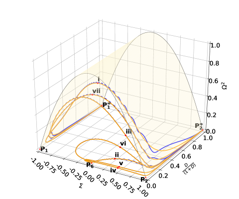
(a) Projections in the space $(\Sigma,D/(1+D),\Omega^{2})$. The surface is given by the constraint $\Omega^{2}=1-\Sigma^{2}$.

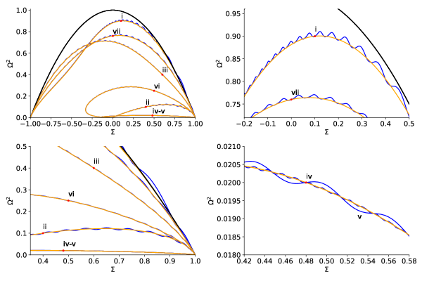
(b) Projection in the space $(\Sigma,\Omega^{2})$. The black line represent the constraint $\Omega^{2}=1-\Sigma^{2}$.

Figure 13: Some solutions of the full system (89) (blue) and time–averaged system (139) (orange) for the KS metric when $\gamma=0$ in the projection $Q=0$. We have used for both systems the initial data sets presented in Table 3.

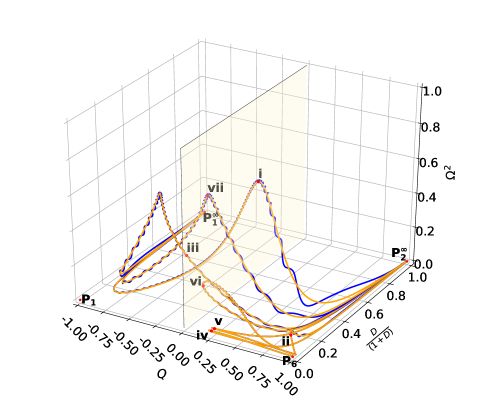
(a) Projections in the space $(Q,D/(1+D),\Omega^{2})$. The surface is given by the constraint $Q=0$.

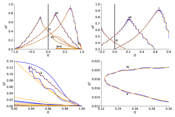
(b) Projection in the space $(Q,\Omega^{2})$. The black line represent the constraint $Q=0$.

Figure 14: Some solutions of the full system (89) (blue) and time–averaged system (139) (orange) for the KS metric when $\gamma=0$ in the projection $\Sigma=0$. We have used for both systems the initial data sets presented in Table 3.

(a) Projections in the space $(\Sigma,D/(1+D),\Omega^{2})$. The surface is given by the constraint $\Omega^{2}=1-\Sigma^{2}$.

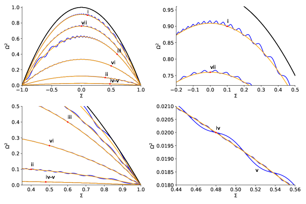
(b) Projection in the space $(\Sigma,\Omega^{2})$. The black line represent the constraint $\Omega^{2}=1-\Sigma^{2}$.

Figure 15: Some solutions of the full system (89) (blue) and time–averaged system (139) (orange) for the KS metric when $\gamma=1$ in the projection $Q=0$. We have used for both systems the initial data sets presented in Table 3.

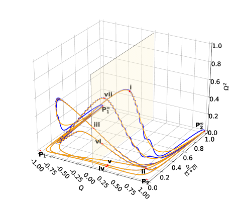
(a) Projections in the space $(Q,D/(1+D),\Omega^{2})$. The surface is given by the constraint $Q=0$.

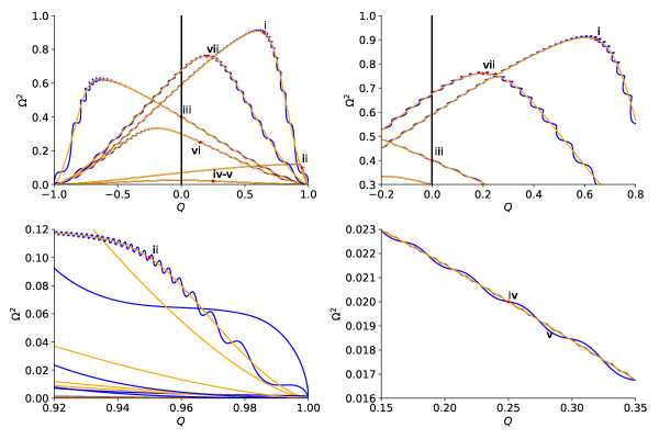
(b) Projection in the space $(Q,\Omega^{2})$. The black line represent the constraint $Q=0$.

Figure 16: Some solutions of the full system (89) (blue) and time–averaged system (139) (orange) for the KS metric when $\gamma=1$ in the projection $\Sigma=0$. We have used for both systems the initial data sets presented in Table 3.

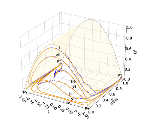
(a) Projections in the space $(\Sigma,D/(1+D),\Omega^{2})$. The surface is given by the constraint $\Omega^{2}=1-\Sigma^{2}$.

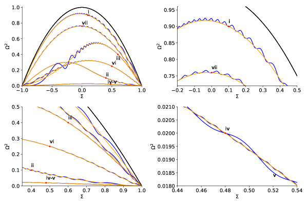
(b) Projection in the space $(\Sigma,\Omega^{2})$. The black line represent the constraint $\Omega^{2}=1-\Sigma^{2}$.

Figure 17: Some solutions of the full system (89) (blue) and time–averaged system (139) (orange) for the KS metric when $\gamma=\frac{4}{3}$ in the projection $Q=0$. We have used for both systems the initial data sets presented in Table 3.

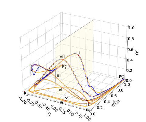
(a) Projections in the space $(Q,D/(1+D),\Omega^{2})$. The surface is given by the constraint $Q=0$.

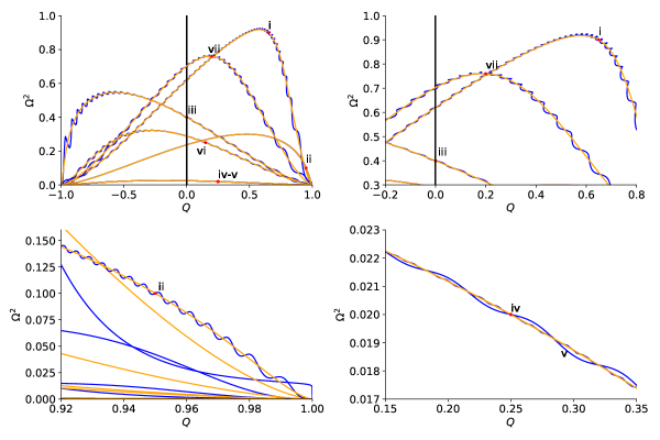
(b) Projection in the space $(Q,\Omega^{2})$. The black line represent the constraint $Q=0$.

Figure 18: Some solutions of the full system (89) (blue) and time–averaged system (139) (orange) for the KS metric when $\gamma=\frac{4}{3}$ in the projection $\Sigma=0$. We have used for both systems the initial data sets presented in Table 3.

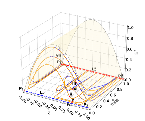
(a) Projections in the space $(\Sigma,D/(1+D),\Omega^{2})$. The surface is given by the constraint $\Omega^{2}=1-\Sigma^{2}$.

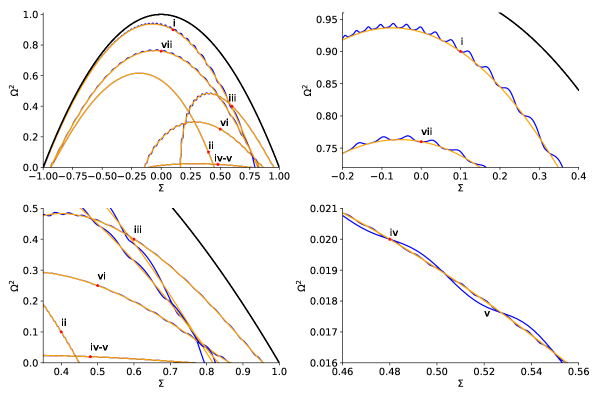
(b) Projection in the space $(\Sigma,\Omega^{2})$. The black line represent the constraint $\Omega^{2}=1-\Sigma^{2}$.

Figure 19: Some solutions of the full system (89) (blue) and time–averaged system (139) (orange) for the KS metric when $\gamma=2$ in the projection $Q=0$. We have used for both systems the initial data sets presented in Table 3.

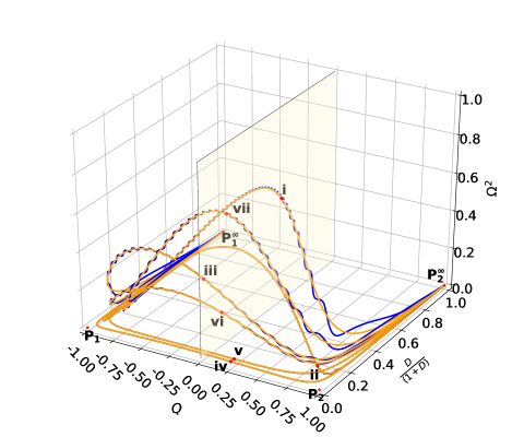
(a) Projections in the space $(Q,D/(1+D),\Omega^{2})$. The surface is given by the constraint $Q=0$.

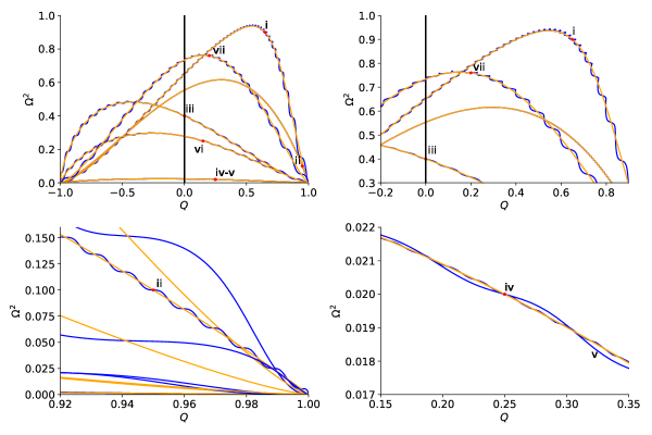
(b) Projection in the space $(Q,\Omega^{2})$. The black line represent the constraint $Q=0$.

Figure 20: Some solutions of the full system (89) (blue) and time–averaged system (139) (orange) for the KS metric when $\gamma=2$ in the projection $\Sigma=0$. We have used for both systems the initial data sets presented in Table 3.

B.2 FLRW metric with positive curvature

For the FLRW metric with positive curvature ($k=+1$) we integrate

1. the full system given by (125).

2. The time–averaged system (157).

For case $\gamma=1$, for which the differential equation for $\Omega$ in time–averaged system (157) becomes trivial, we integrate time–averaged system (163).
Independently of the value of $\gamma$, we use as initial conditions ten data set presented in Table 4, where data sets $I$, $II$, and $VII$ are the symmetrical counterpart with respect to $Q$ of data sets $i$, $ii$, and $vii$.

Table 4: Here we show ten initial data sets for the simulation of full system (125) and time–averaged system (157) for $\gamma\neq 1$ and of system (163) for $\gamma=1$, for the FLRW metric with positive curvature ($k=+1$). All the conditions are chosen in order to fulfill the inequalities $0\leq\Omega\leq 1$ and $-1\leq Q\leq 1$.

Sol.	$D(0)$	$\Omega^{2}(0)$	$Q(0)$	$\varphi(0)$	$t(0)$
i	$0.1$	$0.9$	$0.65$	$0$	$0$
I	$0.1$	$0.9$	$-0.65$	$0$	$0$
ii	$0.1$	$0.1$	$0.95$	$0$	$0$
II	$0.1$	$0.1$	$-0.95$	$0$	$0$
iii	$0.1$	$0.4$	$0$	$0$	$0$
iv	$0.02$	$0.02$	$0.25$	$0$	$0$
v	$0.1$	$0.02$	$0.25$	$0$	$0$
vi	$0.1$	$0.25$	$0.15$	$0$	$0$
vii	$0.1$	$0.76$	$0.2$	$0$	$0$
VII	$0.1$	$0.76$	$-0.2$	$0$	$0$

In Figures 21, 22, 23, and 24 we present projections of some solutions of full system (125) and time–averaged system (157) for $\gamma\neq 1$ and of system (163) for $\gamma=1$ in the $(Q,D/(1+D),\Omega^{2}/(1+\Omega^{2}))$ space with their respective projection when $D=0$. For both systems the same initial data sets from Table 4 were considered. Figures 21(a) and 21(b) show solutions for a fluid corresponding to CC ($\gamma=0$). Figures 22(a) and 22(b) show solutions for a fluid corresponding to dust ($\gamma=1$). Figures 23(a) and 23(b) show solutions for a fluid corresponding to radiation ($\gamma=\frac{4}{3}$). Figures 24(a) and 24(b) show solutions for a fluid corresponding to stiff fluid ($\gamma=2$). Figures 21 and 25 show how solutions of full system (blue lines) follow the track of solutions of averaged system (orange lines) for the whole $D$-range. Figures 22, 23, 24, and 26 are evidence that main theorem presented in Section 4 is fulfilled for FLRW metric with positive curvature ($k=+1$) only when $D$ is bounded. That is, solutions of full system (blue lines) follow the track of solutions of averaged system (orange lines) for the time interval $tD=\mathcal{O}(1)$. However, when $D$ becomes infinite ($T\rightarrow 1$) and for $\gamma\geq 1$ solutions of full system (blue lines) depart from solutions of averaged system (orange lines) as $D$ becomes large. This is clear because when $D$ becomes large, the approximation obtained under the assumption of small $D$ fails.

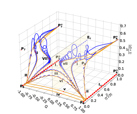
(a) Projections in the space $(Q,D/(1+D),\Omega^{2}/(1+\Omega^{2}))$. The surface is given by the constraint $Q=0$.

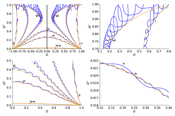
(b) Projection in the space $(Q,\Omega^{2})$. The black line represent the constraint $Q=0$.

Figure 21: Some solutions of the full system (125) (blue) and time–averaged system (157) (orange) for the FLRW metric with positive curvature ($k=+1$) when $\gamma=0$. We have used for both systems the initial data sets presented in Table 4.

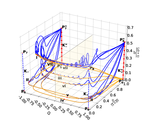
(a) Projections in the space $(Q,D/(1+D),\Omega^{2}/(1+\Omega^{2}))$. The surface is given by the constraint $Q=0$.

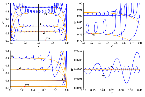
(b) Projection in the space $(Q,\Omega^{2})$. The black line represent the constraint $Q=0$.

Figure 22: Some solutions of the full system (125) (blue) and time–averaged system (163) (orange) for the FLRW metric with positive curvature ($k=+1$) when $\gamma=1$. We have used for both systems the initial data sets presented in Table 4.

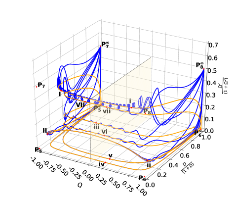
(a) Projections in the space $(Q,D/(1+D),\Omega^{2}/(1+\Omega^{2}))$. The surface is given by the constraint $Q=0$.

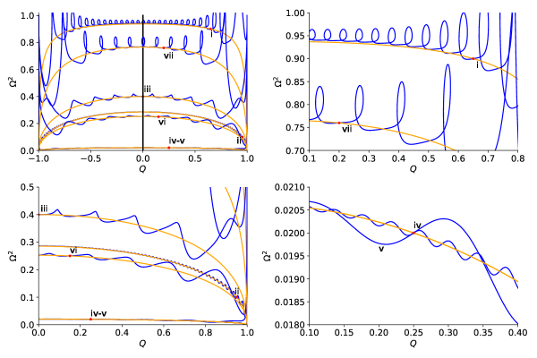
(b) Projection in the space $(Q,\Omega^{2})$. The black line represent the constraint $Q=0$.

Figure 23: Some solutions of the full system (125) (blue) and time–averaged system (157) (orange) for the FLRW metric with positive curvature ($k=+1$) when $\gamma=\frac{4}{3}$. We have used for both systems the initial data sets presented in Table 4.

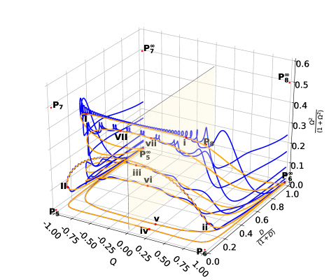
(a) Projections in the space $(Q,D/(1+D),\Omega^{2}/(1+\Omega^{2}))$. The surface is given by the constraint $Q=0$.

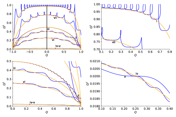
(b) Projection in the space $(Q,\Omega^{2})$. The black line represent the constraint $Q=0$.

Figure 24: Some solutions of the full system (125) (blue) and time–averaged system (157) (orange) for the FLRW metric with positive curvature ($k=+1$) when $\gamma=2$. We have used for both systems the initial data sets presented in Table 4.

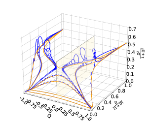
(a) $\gamma=0.1$.

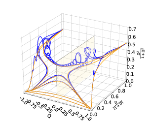
(b) $\gamma=0.3$.

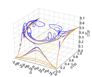
(c) $\gamma=0.4$.

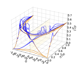
(d) $\gamma=0.5$.

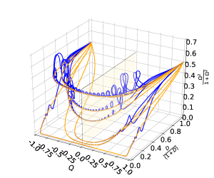
(e) $\gamma=0.7$.

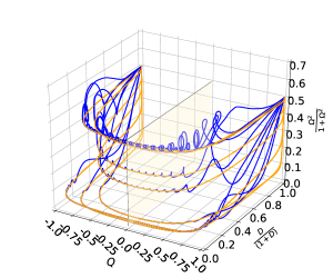
(f) $\gamma=0.9$.

Figure 25: Some solutions of the full system (125) (blue) and time–averaged system (157) (orange) for the closed FLRW metric when $\gamma=0.1$, $0.3$, $0.4$, $0.5$, $0.7$, and $0.9$, respectively; all of them represented in the space $(Q,D/(1+D),\Omega^{2}/(1+\Omega^{2}))$. We have used for both systems the initial data sets presented in Table 4.

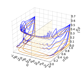
(a) $\gamma=1.1$.

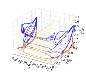
(b) $\gamma=1.3$.

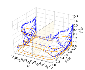
(c) $\gamma=1.4$.

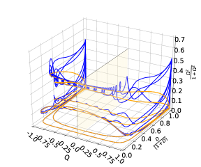
(d) $\gamma=1.5$.

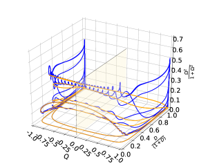
(e) $\gamma=1.7$.

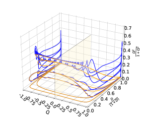
(f) $\gamma=1.9$.

Figure 26: Some solutions of the full system (125) (blue) and time–averaged system (157) (orange) for the closed FLRW metric when $\gamma=1.1$, $1.3$, $1.4$, $1.5$, $1.7$, and $1.9$, respectively; all of them represented in the space $(Q,D/(1+D),\Omega^{2}/(1+\Omega^{2}))$. We have used for both systems the initial data sets presented in Table 4.

References

- [1] S. Foster, Class. Quant. Grav. 15, 3485 (1998)
- [2] J. Miritzis, Class. Quant. Grav. 20, 2981 (2003)
- [3] R. Giambo, F. Giannoni and G. Magli, Gen. Rel. Grav. 41, 21 (2009)
- [4] G. Leon and C. R. Fadragas, Dynamical Systems: And Their Applications (Saarbrücken: LAP Lambert Academic Publishing), arXiv:1412.5701 [gr-qc]
- [5] G. Leon, P. Silveira and C. R. Fadragas, “Phase-space of flat Friedmann-Robertson-Walker models with both a scalar field coupled to matter and radiation,” in Classical and Quantum Gravity: Theory, Analysis and Applications ed V R Frignanni (New York: Nova Science Publisher) ch 10 [arXiv:1009.0689 [gr-qc]]
- [6] C. R. Fadragas and G. Leon Class. Quant. Grav. 31, no. 19, 195011 (2014)
- [7] D. González Morales, Y. Nápoles Alvarez, Quintaesencia con acoplamiento no mínimo a la materia oscura desde la perspectiva de los sistemas dinámicos, Bachelor Thesis, Universidad Central Marta Abreu de Las Villas, Santa Clara, Cuba, 2008
- [8] G. Leon, Class. Quant. Grav. 26, 035008 (2009)
- [9] R. Giambo and J. Miritzis, Class. Quant. Grav. 27, 095003 (2010)
- [10] K. Tzanni and J. Miritzis, Phys. Rev. D 89, no. 10, 103540 (2014) Addendum: [Phys. Rev. D 89, no. 12, 129902 (2014)]
- [11] R. J. van den Hoogen, A. A. Coley and D. Wands, Class. Quant. Grav. 16, 1843 (1999)
- [12] E. J. Copeland, A. R. Liddle and D. Wands, Phys. Rev. D 57, 4686 (1998)
- [13] A. Alho and C. Uggla, J. Math. Phys. 56, no. 1, 012502 (2015)
- [14] R. Giambò, J. Miritzis and A. Pezzola, Eur. Phys. J. Plus 135, no.4, 367 (2020)
- [15] A. Cid, F. Izaurieta, G. Leon, P. Medina and D. Narbona, JCAP 1804, 041 (2018)
- [16] A. H. Guth, Phys. Rev. D 23, 347 (1981)
- [17] A.H. Guth, Adv. Ser. Astrophys. Cosmol. 3, 139 (1987)
- [18] A. D. Linde, Phys. Lett. B 129 (1983), 177-181
- [19] A. D. Linde, Phys. Lett. B 175 (1986), 395-400
- [20] A. D. Linde, [arXiv:hep-th/0205259 [hep-th]]
- [21] A. H. Guth, J. Phys. A 40 (2007), 6811-6826
- [22] E. A. Coddington y Levinson, N. Theory of Ordinary Differential Equations, New York, MacGraw-Hill, (1955)
- [23] J. K. Hale, Ordinary Differential Equations, New York, Wiley (1969)
- [24] D. K. Arrowsmith y C. M. Place, An introduction to dynamical systems, Cambridge University Press, Cambridge, England, (1990)
- [25] S. Wiggins. Introduction to Applied Nonlinear dynamical systems and Chaos. Springer (2003)
- [26] L. Perko, Differential equations and dynamical systems, third edition (Springer-Verlag, New York, 2001).
- [27] V.I. Arnold, Ordinary differential equations. Cambridge: M.I.T. Press., 1973
- [28] M. W. Hirsch and S. Smale. Differential equations, dynamical systems and linear algebra. New York: Academic Press (1974)
- [29] J. Hale. Ordinary differential equations. Malabar, Florida: Robert E. Krieger Publishing Co., Inc. (1980)
- [30] Lasalle, J. P., J. Diff. Eq., 4, pp. 57-65, 1968
- [31] B. Aulbach, Continuous and Discrete Dynamics near Manifolds of Equilibria (Lecture Notes in Mathematics No. 1058, Springer, 1984)
- [32] R. Tavakol, Introduction to dynamical systems, ch 4. Part one, pp. 84–98, Cambridge University Press, Cambridge, England, (1997)
- [33] A.A. Coley, 2003, Dynamical systems and cosmology (Kluwer Academic, Dordrecht: ISBN 1-4020-1403-1). pages 7-26
- [34] A. A. Coley, Introduction to Dynamical Systems. Lecture Notes for Math 4190/5190 (1994)
- [35] A. A. Coley, gr-qc/9910074
- [36] Bassemah Alhulaimi (2017), Einstein-Aether Cosmological Scalar Field Models (Phd Thesis, Dalhousie University)
- [37] V. G. LeBlanc, D. Kerr and J. Wainwright, Class. Quant. Grav. 12, 513 (1995)
- [38] J. M. Heinzle and C. Uggla, Class. Quant. Grav. 27, 015009 (2010)
- [39] F. Dumortier and R. Roussarie (1995) “Canard cycles and center manifolds”, (Memoirs of the American Mathematical Society, 577)
- [40] N. Fenichel (1979) Geometric singular perturbation theory for ordinary differential equations. Journal of Differential Equations 31, 53-98
- [41] G. Fusco and J.K. Hale, Journal of Dynamics and Differential Equations 1, 75 (1988)
- [42] N. Berglund and B. Gentz, Noise-Induced Phenomena in Slow-Fast Dynamical Systems, Series: Probability and Applications, Springer-Verlag: London, (2006)
- [43] M. H. Holmes (2013) “Introduction to Perturbation Methods”, (Springer Science+Business Media New York, ISBN 978-1-4614-5477-9)
- [44] Jirair Kevorkian, J.D. Cole (1981) “Perturbation Methods in Applied Mathematics” (Applied Mathematical Sciences Series, Volume 34, Springer-Verlag New York eBook ISBN 978-1-4757-4213-8)
- [45] Ferdinand Verhulst, (2000) “Methods and Applications of Singular Perturbations: Boundary Layers and Multiple Timescale Dynamics” (Springer-Verlag New York, ISBN 978-0-387-22966-9)
- [46] G. Leon, E. González, S. Lepe, C. Michea and A. D. Millano, Eur. Phys. J. C 81, 414 (2021)
- [47] G. Leon, S. Cuéllar, E. González, S. Lepe, C. Michea and A. D. Millano, Eur. Phys. J. C 81, 489 (2021)
- [48] D. Fajman, G. Heißel and M. Maliborski, Class. Quant. Grav. 37, no.13, 135009 (2020)
- [49] A. Mitsopoulos, M. Tsamparlis and A. Paliathanasis, Mod. Phys. Lett. A 34 (2019) no.39, 1950326
- [50] A. Paliathanasis, L. Karpathopoulos, A. Wojnar and S. Capozziello, Eur. Phys. J. C 76 (2016) no.4, 225
- [51] G. Leon and F. O. F. Silva 2021 Class. Quantum Grav. 38 015004
- [52] G. Leon and F. O. F. Silva, [arXiv:2003.03563 [gr-qc]]
- [53] G. Leon and F. O. F. Silva, Class. Quant. Grav. 37 (2020) no.24, 245005
- [54] G. Leon and F. O. F. Silva, [arXiv:1912.09856 [gr-qc]]
- [55] J. Wainwright and G. F. R. Ellis, Eds. Dynamical Systems in Cosmology. Cambridge Univ. Press, Cambridge, 1997
- [56] H. van Elst and C. Uggla, Class. Quant. Grav. 14 (1997), 2673-2695 doi:10.1088/0264-9381/14/9/021 [arXiv:gr-qc/9603026 [gr-qc]]
- [57] H. Stephani, D. Kramer, M. A. H. MacCallum, C. A. Hoenselaers, E. Herlt, Exact solutions of Einstein’s field equations, second edition (Cambridge University Press, Cambridge, 2003)
- [58] A. A. Coley, W. C. Lim and G. Leon, [arXiv:0803.0905 [gr-qc]]
- [59] E. A. Milne, “Relativity, Gravitation and World Structure”, Oxford University Press, 1935.
- [60] S. M. Carroll, “Spacetime and Geometry,” San Francisco, USA: Addison-Wesley (2004) 513 p
- [61] V. Mukhanov, “Physical Foundations of Cosmology,” UK: Cambridge University Press (2005), 27p
- [62] C. W. Misner, K. S. Thorne and J. A. Wheeler, “Gravitation,” San Francisco 1973, 1279p
- [63] M. Sharma, M. Shahalam, Q. Wu and A. Wang, JCAP 1811, 003 (2018)
- [64] L. McAllister, E. Silverstein, A. Westphal and T. Wrase, JHEP 09 (2014), 123
- [65] A. D. Rendall, Class. Quant. Grav. 24, 667 (2007)
- [66] G. D’Amico, T. Hamill and N. Kaloper, Phys. Rev. D 94 (2016) no.10, 103526
- [67] A. B. Balakin and A. F. Shakirzyanov, Universe 6 (2020) no.11, 192
- [68] S. Chakraborty, E. González, G. Leon and B. Wang, [arXiv:2107.04651 [gr-qc]].
- [69] D. Fajman, G. Heißel and J. W. Jang, Class. Quant. Grav. 38 (2021) no.8, 085005
- [70] A. S. Kompaneets and A. S. Chernov, Zh. Eksp. Teor. Fiz. (J. Exptl. Theoret. Phys. (U.S.S.R.)) 47 (1964) 1939 [Sov. Phys. JETP 20, 1303 (1965)]
- [71] R. Kantowski and R. K. Sachs, J. Math. Phys. 7, 443 (1966)
- [72] A. B. Burd and J. D. Barrow, Nucl. Phys. B 308, 929 (1988)
- [73] J. Yearsley and J. D. Barrow, Class. Quant. Grav. 13, 2693 (1996)
- [74] M. Thorsrud, B.D. Normann and T.S. Pereira, Class. Quantum Grav. 37, 065015 (2020)
- [75] S. Byland and D. Scialom, Phys. Rev. D 57, 6065-6074 (1998)
- [76] C. R. Fadragas, G. Leon and E. N. Saridakis, Class. Quant. Grav. 31 (2014) 07501
- [77] C. B. Collins, J. Math. Phys. 18, 2116 (1977)
- [78] E. Weber, J. Math. Phys. 25, 3279 (1984)
- [79] O. Gron, J. Math. Phys. 27, 1490-1491 (1986)
- [80] D. Lorenz-Petzold, Phys. Lett. B 149, 79-81 (1984)
- [81] J. D. Barrow and M. P. Dabrowski, Phys. Rev. D 55, 630-638 (1997)
- [82] D. Clancy, J. E. Lidsey and R. K. Tavakol, Class. Quant. Grav. 15, 257-272 (1998)
- [83] A. D. Rendall and K. P. Tod, Class. Quant. Grav. 16, 1705-1726 (1999)
- [84] D. M. Solomons, P. Dunsby and G. Ellis, Class. Quant. Grav. 23, 6585-6597 (2006)
- [85] S. Calogero and J. M. Heinzle, Physica D 240, 636-669 (2011)
- [86] G. Leon and E. N. Saridakis, Class. Quant. Grav. 28, 065008 (2011)
- [87] G. Leon and A. A. Roque, JCAP 05, 032 (2014)
- [88] F. G. Alvarenga, R. Fracalossi, R. C. Freitas and S. V. B. Gonçalves, Braz. J. Phys. 48, no.4, 370-379 (2018)
- [89] M. Zubair and S. M. Ali Hassan, Astrophys. Space Sci. 361, no.4, 149 (2016)
- [90] J. Latta, G. Leon and A. Paliathanasis, JCAP 11, 051 (2016)
- [91] U. Camci, A. Yildirim and I. Basaran Oz, Astropart. Phys. 76, 29-37 (2016)
- [92] S. Jamal and G. Shabbir, Eur. Phys. J. Plus 132, no.2, 70 (2017)
- [93] R. J. Van Den Hoogen, A. A. Coley, B. Alhulaimi, S. Mohandas, E. Knighton and S. O’Neil, JCAP 11, 017 (2018)
- [94] J. D. Barrow and A. Paliathanasis, Eur. Phys. J. C 78, no.9, 767 (2018)
- [95] D. Fajman and G. Heißel, Class. Quant. Grav. 36, no.13, 135002 (2019)
- [96] G. Leon, A. Paliathanasis and N. Dimakis, Eur. Phys. J. C 80, no.12, 1149 (2020)
- [97] M. de Cesare, S. S. Seahra and E. Wilson-Ewing, JCAP 07, 018 (2020)
- [98] B. J. Carr and A. A. Coley, Phys. Rev. D 62 (2000), 044023
- [99] B. J. Carr, A. A. Coley, M. Goliath, U. S. Nilsson and C. Uggla, Class. Quant. Grav. 18 (2001), 303-324
- [100] U. S. Nilsson and C. Uggla, Annals Phys. 286 (2001), 292-319
- [101] B. J. Carr and A. A. Coley, Class. Quant. Grav. 16 (1999), R31-R71
- [102] M. Goliath, U. S. Nilsson and C. Uggla, Class. Quant. Grav. 15 (1998), 2841
- [103] A. Alho, J. Hell and C. Uggla, Class. Quant. Grav. 32 (2015) no.14, 145005
- [104] A. Alho, V. Bessa and F. C. Mena, J. Math. Phys. 61 (2020) no.3, 032502
- [105] A. S. Eddington, Mon. Not. Roy. Astron. Soc. 90 (1930), 668-678
- [106] E. R. Harrison, Rev. Mod. Phys. 39 (1967), 862-882
- [107] G. W. Gibbons, Nucl. Phys. B 292 (1987), 784-792
- [108] G. W. Gibbons, Nucl. Phys. B 310 (1988), 636-642
- [109] A. B. Burd and J. D. Barrow, Nucl. Phys. B 308 (1988), 929-945 [erratum: Nucl. Phys. B 324 (1989), 276-276]
- [110] H. Noh, J. c. Hwang and J. D. Barrow, Phys. Rev. D 101 (2020) no.12, 123527
- [111] J. D. Barrow and C. G. Tsagas, Class. Quant. Grav. 26 (2009), 195003
- [112] J. D. Barrow, G. F. R. Ellis, R. Maartens and C. G. Tsagas, Class. Quant. Grav. 20 (2003), L155-L164
- [113] J. M. Heinzle, N. Rohr and C. Uggla, Phys. Rev. D 71 (2005), 083506
- [114] J. M. Heinzle, N. Rohr and C. Uggla, Phys. Rev. D 74 (2006), 061502
- [115] H. P. de Oliveira, I. D. Soares and T. J. Stuchi, Phys. Rev. D 56 (1997), 730-740
- [116] R. Barguine, H. P. de Oliveira, I. D. Soares and E. V. Tonini, Phys. Rev. D 63 (2001), 063502
- [117] H. P. De Oliveira, A. M. Ozorio de Almeida, I. D. Soares and E. V. Tonini, Phys. Rev. D 65 (2002), 083511
- [118] I. D. Soares and T. J. Stuchi, Phys. Rev. D 72 (2005), 083516 [erratum: Phys. Rev. D 73 (2006), 069901]