Geometrized effective-one-body formalism for extreme-mass-ratio limits: Generic orbits

Abstract

Compact objects inspiraling into supermassive black holes, known as extreme-mass-ratio inspirals, are an important source for future space-borne gravitational-wave detectors. When constructing waveform templates, usually the adiabatic approximation is employed to treat the compact object as a test particle for a short duration, and the radiation reaction is reflected in the changes of the constants of motion. However, the mass of the compact object should have contributions to the background. In the present paper, employing the effective-one-body formalism, we analytically calculate the trajectories of a compact object around a massive Kerr black hole with generally three-dimensional orbits and express the fundamental orbital frequencies in explicit forms. In addition, by constructing an approximate “constant” similar to the Carter constant, we transfer the dynamical quantities such as energy, angular momentum, and the “Carter constant” to the semilatus rectum, eccentricity, and orbital inclination with mass-ratio corrections. The linear mass-ratio terms in the formalism may not be sufficient for accurate waveforms, but our analytical method for solving the equations of motion could be useful in various approaches to building waveform models.

I Introduction

One of the most promising and rewarding sources of gravitational waves for low-frequency, space-based gravitational-wave (GW) detectors—such as the future Laser Interferometer Space Antenna(LISA) lisa , Taiji hu2017taiji and Tian-Qin luo2016tianqin —are the so-called extreme-mass-ratio inspirals (EMRIs) amaro2007intermediate ; babak2017science ; berry2019unique , which are compact objects (COs) such as neutron stars or stellar-mass (or stellar origin) black holes (SOBHs) inspiraling into supermassive black holes (SMBHs) in the mass range $10^{5}$-$10^{7}\,{\rm M_{\odot}}$.

The majority of observed EMRI events are expected to be SOBH-SMBH mergers; this is partly due to mass segregation concentrating heavier BHs in the Galactic center and partly because their louder intrinsic amplitude enables them to be detected out to greater distances. The small CO is usually approximated as a test particle, and over the short orbital time scale follows a nearly geodesic trajectory in the background metric of the SMBH. The system radiates GWs at harmonics of the geodesic frequencies, so the GW frequency spectrum encodes details of the instantaneous geodesic trajectory.

Though the signals from EMRIs are usually very weak, after one year of observation the signal-to-noise ratio may be enough to be detected  amaro2007intermediate . To detect this kind of long duration signals, the requirement on the accuracy of waveform templates is that the dephasing should be less than a few radians after $10^{5}$ cycles gair2013testing ; babak2017science .

Nowadays, there are several kinds of EMRI templates. The first kind uses Teukolsky equations Teukolsky and treats COs as test particles (omitting the mass in their conservation dynamics part) and thus they just extract a snapshot waveform; however, accurate Teukolsky-based waveforms are computationally expensive to generate. Another kind uses the post-Newtonian (PN) fluxes approximation to describe the evolution of orbital parameters with gravitational radiation reaction, in particular the so-called kludge waveforms barack2004lisa ; babak2007kludge ; chua2017augmented . The third kind considers the correction due to the small mass by using the effective-one-body (EOB) formalism, but does not consider the spin of the small object, such as in circular orbits with PN waveforms yunes2010modeling ; yunes2011extreme and the Teukolsky-based waveforms han2011constructing ; han2014gravitational . The kludge models can generate the waveforms quickly for three-dimensional (3D) orbits, but they take the COs as test particles in the orbital motion even though they include the radiation reaction.

If the time scale of GW radiation is much larger than that of the orbital motion, then at a given instant the properties of motion can be calculated from a conservative equation $\ddot{x}^{\mu}+^{B}\Gamma^{\mu}_{\rho\sigma}\dot{x}^{\mu}\dot{x}^{\nu}=0+O(\nu)+O(\nu^{2})+\cdots$. Here the label “B” represents the background field of the massive body. In popular EMRI template models, like AAK barack2004lisa , NK babak2007kludge , AAK chua2017augmented , XSPEG xin2019gravitational etc, the mass-ratio corrections in the conservative dynamics are omitted, i.e., the right-hand side of the equation is exactly zero. This is just the geodesic equation of a test particle around a massive black hole. The test particle–adiabatic approximation (adiabatic model) makes the problem much simpler, but induces errors in the GW simulation. As in Eq.(74) of Ref.barack2018self , the mass ratio expansion to the phase evolution is

$$\phi(t)=\frac{1}{\nu}[\phi_{(0)}+\nu\phi_{(1)}+O(\nu^{2})].$$ (1)

An EMRI model that captures the leading-order term $\phi_{(0)}$ is called an adiabatic model. The calculation of $\phi_{(0)}$ requires only the averaged dissipative first-order self-force (in the mass-ratio expansion) that is fully equivalent to the fluxes, and some literature states that in general it may be accurate enough for detecting EMRI signals using LISA hughes2018adiabatic . The next-to-leading-order term, which includes both the dissipative and conservative pieces of the first-order self-force as well as the averaged dissipative piece of the second-order self-force. The post-1 adiabatic phase is required for the parameter estimation of EMRIs hughes2018adiabatic . In the present paper, we mainly focus on the conservation dynamics part of EMRI, and try to analytically solve the equation of motion which includes the first-order mass-ratio corrections. The mass-ratio terms we use may not be enough for final EMRI waveforms, so the aim of this paper is not to construct the waveform template, but rather to demonstrate the method for the analytical solution of orbits. Our method should be useful once there are some more precise self-force corrections.

The EOB formalism, by including the mass-ratio corrections up to a certain order in the PN expansion, can well describe the dynamical evolution of binary black holes buonanno1999eff ; buonanno2000transition , and is widely used to construct the waveform templates for LIGO taracchini2014effective ; buonanno2007approaching ; purrer2016frequency ; husa2016frequency ; khan2016frequency ; chu2016accuracy ; kumar2016accuracy ; pan2014inspiral . Most of these models only consider the circular-orbit cases. An eccentric EOB numerical relativity waveform template for spinning black holes was developed  cao2017waveform , but the orbits were not geometrized and the orbital parameters were not well defined. Recently, an analytically eccentric EOB formalism for Schwarzschild BHs was given hinderer2017foundations . In a previous work zc2020 , we present an analytically equatorial-eccentric EOB formalism for spinning cases in the extreme-mass-ratio limit. Note that the EOB formalism’s correction in the extreme-mass-ratio limit has not been guaranteed. However, as stated in Ref.albanesi2021effective , the extreme-mass-ratio limit plays a pivotal role in the EOB development, especially for what concerns waveforms and fluxes, which can be informed by and compared with numerical results  Nagar:2006xv ; Damour:2007xr ; Bernuzzi:2010ty ; Bernuzzi:2011bc ; Bernuzzi:2010xj ; Bernuzzi:2011aj ; Harms:2014an ; Nagar:2014kha ; Harms:2015ixa ; Harms:2016ctx ; Lukes:2017st ; Nagar:2019wrt . In addition, the EOB formalism with the extreme-mass-ratio limit should be improved due to a lot of works dedicated to analytically calculating gravitational self-force terms and providing comparisons with numerical results  Damour:2009sm ; Barack:2010ny ; Akcay:2012ea ; Bini:2014ica ; Bini:2015mza ; Akcay:2015pjz ; Barack:2019agd .

It is well known that the orbits of EMRIs could be highly eccentric babak2017science with orbital inclination (orbital plane procession), and the supermassive black hole in the center should be spinning in general. In the present paper, we extend the previous work by Hinderer and Babak hinderer2017foundations and ourselves  zc2020 to the inclined-eccentric orbits in the Kerr background with the extreme-mass-ratio limit. We analytically transfer the original EOB dynamical equations to geometric kinetic motion with the semilatus rectum $p$, eccentricity $e$ and orbital inclination $\iota$ as the orbital parameters, together with three phase variables associated with the spatial geometry of the radial, azimuthal, and polar motion denoted by $(\xi,\phi,\chi)$. Because of the extremely small mass ratio,we omit the spin of the effective small body, and thus the very complicated spin-spin coupling terms disappear but maintain enough accuracy.

An important feature of the dynamics of an extrememass-ratio binary system in a bounded inclined-eccentric orbit is that the orbit can be characterized by three frequencies: the radial frequency $\omega_{r}$ associated with the libration between the apoapsis and periapsis, the polar frequency $\omega_{\theta}$ associated with the libration between $\theta_{min}$ and $\pi-\theta_{min}$, and the azimuthal rotational frequency $\omega_{\phi}$. Once these three frequencies and orbital parameters are obtained, the frequency of GWs can be obtained and may be encoded in the Teukolsky equation to get accurate waveforms han2010gravitational ; han2011constructing ; han2014gravitational ; han2017excitation ; cai2016gravitational ; yang2019testing ; cheng2019highly .

The organization of this paper is as follows. The basic knowledge of EOB formalism is introduced in the following section. In Sec. III, we reparametrize the original spinning EOB dynamical description to a geometric formalism in the more efficient reparametrized terms of $(p,~{}e,~{}\iota,~{}\xi,~{}\chi,~{}\phi)$. We analytically express the fundamental frequencies in three integrals with two parameters: $\xi$ and $\chi$. In particular, we investigate the influence of the mass ratio on the detection of EMRIs. We also give the general forms for the evolution of orbital parameters with gravitational radiation reaction. Finally, the last section contains our conclusions and discussions.

Throughout this paper we use geometric units $G=c=1$, the units of time and length are the mass of system $M$, and the units of linear and angular momentum are $\mu$ and $\mu M$, respectively, where $\mu$ is the reduced mass of the effective body.

II Effective-one-body Hamiltonian

The EOB formalism was originally introduced in Refs. buonanno1999eff ; buonanno2000transition to describe the evolution of a binary system. We start by considering an EMRI system with a central Kerr black hole $m_{1}$ and inspiraling object $m_{2}$ (we assume that it is nonspinning for simplicity, $m_{2}\ll m_{1}$). For the moment, we neglect the radiation-reaction effects and focus on purely geodesic motion. The conservative orbital dynamics is derived via Hamilton’s equations using the EOB Hamiltonian

$$H_{\rm EOB}=M\sqrt{1+2\nu(\hat{H}_{\rm eff}-1)}\,,$$ (2)

where $M=m_{1}+m_{2}$, $\nu=m_{1}m_{2}/M^{2}$, $\mu=\nu M$ and the reduced effective Hamiltonian $\hat{H}_{\rm eff}=H_{\rm eff}/\mu$. The deformed Kerr metric is given by barausse2010improved

$$g^{tt} = -\frac{\Lambda_{t}}{\Delta_{t}\,\Sigma}\,,$$ (3a)

$$g^{rr} = \frac{\Delta_{r}}{\Sigma}\,,$$ (3b)

$$g^{\theta\theta} = \frac{1}{\Sigma}\,,$$ (3c)

$$g^{\phi\phi} = \frac{1}{\Lambda_{t}}\left(-\frac{\widetilde{\omega}_{\rm fd}^{2}}{\Delta_{t}\,\Sigma}+\frac{\Sigma}{\sin^{2}\theta}\right)\,,$$ (3d)

$$g^{t\phi} = -\frac{\widetilde{\omega}_{\rm fd}}{\Delta_{t}\,\Sigma}\,.$$ (3e)

The quantities $\Sigma$, $\Delta_{t}$, $\Delta_{r}$, $\Lambda_{t}$, and $\widetilde{\omega}_{\rm fd}$ in Eqs. (3a)-(3e) are given by

$$\Sigma = r^{2}+a^{2}\cos^{2}\theta\,,$$ (4a)

$$\Delta_{t} = r^{2}\,\left[A(u)+\frac{a^{2}}{M^{2}}\,u^{2}\right]\,,$$ (4b)

$$\Delta_{r} = \Delta_{t}\,D^{-1}(u)\,,$$ (4c)

$$\Lambda_{t} = \left(r^{2}+a^{2}\right)^{2}-a^{2}\Delta_{t}\sin^{2}\theta\,,$$ (4d)

$$\widetilde{\omega}_{\rm fd} = 2a\,M\,r+\omega_{1}^{\rm fd}\,\nu\,\frac{aM^{3}}{r}+\omega_{2}^{\rm fd}\,\nu\,\frac{Ma^{3}}{r}\,,$$ (4e)

where $a=|\bm{S}_{\rm{Kerr}}|/M$ is the effective Kerr parameter and $u=M/r$. The values of $\omega_{1}^{\rm fd}$ and $\omega_{2}^{\rm fd}$ given by a preliminary comparison of EOB model with numerical relativity results are about $-10$ and $20$ rezzolla2008final ; barausse2009predicting , and the metric potentials $A$ and $D$ for the EOB model are given as follows.

The log-resummed, calibrated A potential is given by the expression from APPENDIX A of Ref. steinhoff2016Apotential

$$A(u) = \Delta_{u}-\frac{a^{2}}{M^{2}}u^{2},$$ (5)

$$\Delta_{u} = \bar{\Delta}_{u}\left(\Delta_{0}\nu+\nu\log\left(\Delta_{5}u^{5}+\Delta_{4}u^{4}+\Delta_{3}u^{3}+\Delta_{2}u^{2}+\Delta_{1}u+1\right)+1\right),$$ (6)

with

$$\bar{\Delta}_{u} =\frac{a^{2}u^{2}}{M^{2}}+\frac{1}{(K\nu-1)^{2}}+\frac{2u}{K\nu-1},$$ (7a)

$$\Delta_{5} =(K\nu-1)^{2}\bigg{[}\frac{64}{5}\log(u)+\left(-\frac{1}{3}a^{2}\left(\Delta_{1}^{3}-3\Delta_{1}\Delta_{2}+3\Delta_{3}\right)\right.$$

$$-\frac{\Delta_{1}^{5}-5\Delta_{1}^{3}\Delta_{2}+5\Delta_{1}^{2}\Delta_{3}+5\Delta_{1}\Delta_{2}^{2}-5\Delta_{2}\Delta_{3}-5\Delta_{4}\Delta_{1}}{5(K\nu-1)^{2}}$$

$$\left.+\frac{\Delta_{1}^{4}-4\Delta_{1}^{2}\Delta_{2}+4\Delta_{1}\Delta_{3}+2\Delta_{2}^{2}-4\Delta_{4}}{2K\nu-2}+\frac{2275\pi^{2}}{512}+\frac{128\gamma}{5}-\frac{4237}{60}+\frac{256\log(2)}{5}\right)\bigg{]},$$ (7b)

$$\Delta_{4} =\frac{1}{96}\bigg{[}8\left(6a^{2}\left(\Delta_{1}^{2}-2\Delta_{2}\right)(K\nu-1)^{2}+3\Delta_{1}^{4}+\Delta_{1}^{3}(8-8K\nu)\right.$$

$$\left.-12\Delta_{1}^{2}\Delta_{2}+12\Delta_{1}(2\Delta_{2}K\nu-2\Delta_{2}+\Delta_{3})\right)$$

$$+48\Delta_{2}^{2}-64(K\nu-1)(3\Delta_{3}-47K\nu+47)-123\pi^{2}(K\nu-1)^{2}\bigg{]},$$ (7c)

$$\Delta_{3} =-a^{2}\Delta_{1}(K\nu-1)^{2}-\frac{\Delta_{1}^{3}}{3}+\Delta_{1}^{2}(K\nu-1)+\Delta_{1}\Delta_{2}-2(K\nu-1)(\Delta_{2}-K\nu+1),$$ (7d)

$$\Delta_{2} =\frac{1}{2}\left(\Delta_{1}(\Delta_{1}-4K\nu+4)-2a^{2}\Delta_{0}(K\nu-1)^{2}\right),$$ (7e)

$$\Delta_{1} =-2(\Delta_{0}+K)(K\nu-1),$$ (7f)

$$\Delta_{0} =K(K\nu-2),$$ (7g)

where $$K$$ is a calibration parameter tuned to numerical-relativity simulations whose most recently updated value was determined in Eq. (4.8) of Ref. bohe2017improved

$$K=267.788\nu^{3}-126.687\nu^{2}+10.2573\nu+1.7336$$ (7h)

The $D$ potential is

$$D^{-1}(u) =1+\log\left[D_{\rm Taylor}\right]$$

$$D_{\rm Taylor} =1+6\nu u^{2}+2\nu u^{3}(26-3\nu).$$ (8a)

III Geometrization of the conservative EOB dynamics

The EOB Hamiltonian in Eq. (2) is canonically transformed and subsequently mapped to an effective Hamiltonian $H_{\rm eff}$ describing a particle of effective mass $\mu$ and effective spin $S_{*}=aM(m_{2}/m_{1})$, moving in a deformed Kerr metric of mass $M$ and effective spin $S_{\rm Kerr}=aM$, and the effective Hamiltonian is given by barausse2010improved ; Barausse2011Extending ; Taracchini2012Prototype

$$H_{\rm eff}=H_{\rm NS}+H_{\rm S}-\frac{\nu}{2r^{3}}S_{*}^{2}\,,$$ (9)

where the first part is just the Hamiltonian of a nonspinning particle in the deformed-Kerr metric with the mass-ratio correction. When $\nu\rightarrow 0$, this part goes back to the test-particle limit in Kerr spacetime. The forms of $H_{s}$ and $S_{*}$ are quite trivial; readers can refer to Barausse2011Extending for details. For EMRIs, due to the small mass-ratio $\nu\sim 10^{-7}\sim 10^{-4}$, as we have shown in zc2020 , the last two terms in Eq.(9) can be neglected without loss of accuracy because they are two orders less than the mass ratio. The Hamiltonian equations for the orbital motion are

$$\frac{d\bm{r}}{d{t}}=\frac{\partial{H}_{\mathrm{EOB}}}{\partial\bm{P}}\,,\qquad\frac{d\bm{P}}{d{t}}=-\frac{\partial{H}_{\mathrm{EOB}}}{\partial\bm{r}}\,.$$ (10)

In form, the above differential equations are coupling each other, especially for radial $r$ and polar $\theta$ equations. Though the numerical integral can give accurate trajectories, analytical ones with geometrized parameters will be valuable for revealing the properties of motion. In the section, we follow the procedure of the test-particle case, decouple the motion in the $r$ and $\theta$ directions, and give a geometrized formalism to replace the dynamical equation(10).

III.1 Semi-Carter “constant” in deformed Kerr spacetime

The effective one-body dynamics was given by a Hamilton-Jacobi equation of the form damour2001coalescence

$$g^{\alpha\beta}P_{\alpha}P_{\beta}+\frac{Q_{4}M^{2}P_{r}^{4}}{r^{2}\mu^{2}}+\mu^{2}=0\,.$$ (11)

The function ${Q}_{4}=2(4-3\nu)\nu$ damour2000determination represents a nongeodesic term that appears at 3PN order. We omit this term in the following calculations because it is next-to-leading order in the mass ratio and the above equation cannot be separated if we retain this term. We use the deformed Kerr metric components (3a)-(3e) to bring Eq. (11) into the concrete form

$$-\mu^{2}\Sigma = -\frac{\left(r^{2}+a^{2}\right)^{2}-a^{2}\sin^{2}\theta(r^{2}A(u)+a^{2})}{r^{2}A(u)+a^{2}}P_{t}^{2}-2\frac{\widetilde{\omega}_{\rm fd}}{r^{2}A(u)+a^{2}}P_{t}P_{\phi}+\Delta_{r}P_{r}^{2}$$ (12)

$$+P_{\theta}^{2}+\frac{1}{\left(r^{2}+a^{2}\right)^{2}-a^{2}\sin^{2}\theta(r^{2}A(u)+a^{2})}\left(\frac{(r^{2}+a^{2}\cos^{2}\theta)^{2}}{\sin^{2}\theta}-\frac{{\widetilde{\omega}_{\rm fd}}^{2}}{r^{2}A(u)+a^{2}}\right)P_{\phi}^{2}\,,$$

where $P_{r}$, $P_{\phi}$, and $P_{\theta}$ are the canonical radial, azimuthal, and polar angular momentum. From the symmetries we immediately obtain two constants of motion corresponding to the conservation of energy, $H_{\rm eff}$, and angular momentum about the symmetry axis, $L_{z}$; thus, we have

$$P_{t} = -H_{\rm eff}\,,$$ (13a)

$$P_{\phi} = L_{z}\,,$$ (13b)

Then, Eq. (12) becomes

$$-\Sigma = -\frac{\left(r^{2}+a^{2}\right)^{2}-a^{2}\sin^{2}\theta(r^{2}A(u)+a^{2})}{r^{2}A(u)+a^{2}}\hat{H}_{\rm eff}^{2}+2\frac{\widetilde{\omega}_{\rm fd}}{r^{2}A(u)+a^{2}}\hat{H}_{\rm eff}\hat{L}_{z}+\Delta_{r}\hat{P_{r}}^{2}$$ (14)

$$+\hat{P_{\theta}}^{2}+\frac{1}{\left(r^{2}+a^{2}\right)^{2}-a^{2}\sin^{2}\theta(r^{2}A(u)+a^{2})}\left(\frac{(r^{2}+a^{2}\cos^{2}\theta)^{2}}{\sin^{2}\theta}-\frac{{\widetilde{\omega}_{\rm fd}}^{2}}{r^{2}A(u)+a^{2}}\right)\hat{L_{z}}^{2}\,,$$

where we have defined the reduced momenta $\hat{P}_{r}=P_{r}/\mu$, $\hat{P}_{\theta}=P_{\theta}/\mu$, and $\hat{L}_{z}=L_{z}/\mu$. It is convenient to rewrite this expression as

$$-\Sigma = -\frac{\left(a\hat{L_{z}}-\left(r^{2}+a^{2}\right)\hat{H}_{\rm eff}\right)^{2}}{r^{2}A(u)+a^{2}}+\frac{\left(\hat{L_{z}}-a\sin^{2}\theta\hat{H}_{\rm eff}\right)^{2}}{\sin^{2}\theta}+\Delta_{r}\hat{P_{r}}^{2}+\hat{P_{\theta}}^{2}$$ (15)

$$+2\frac{\widetilde{\omega}_{\rm fd}+ar^{2}\left(A(u)-1\right)}{r^{2}A(u)+a^{2}}\hat{H}_{\rm eff}\hat{L_{z}}-\frac{{\widetilde{\omega}_{\rm fd}}^{2}-a^{2}r^{4}\left(A(u)-1\right)^{2}}{\left(r^{2}A(u)+a^{2}\right)\left(\left(r^{2}+a^{2}\right)^{2}-a^{2}\sin^{2}\theta(r^{2}A(u)+a^{2})\right)}\hat{L_{z}}^{2}\,,$$

and solving this equation by separation of variables gives

$$\left(\frac{\hat{L_{z}}}{\sin\theta}\!-\!a\hat{H}_{\rm eff}\sin\theta\right)^{2}\!+\!\hat{P_{\theta}}^{2}\!+\!a^{2}\cos^{2}\theta\!=\!\frac{\left(a\hat{L_{z}}-\left(r^{2}+a^{2}\right)\hat{H}_{\rm eff}\right)^{2}}{r^{2}A(u)+a^{2}}-\Delta_{r}\hat{P_{r}}^{2}-r^{2}-2\frac{\widetilde{\omega}_{\rm fd}+ar^{2}\left(A(u)-1\right)}{r^{2}A(u)+a^{2}}\hat{H}_{\rm eff}\hat{L_{z}}+F(r,\theta)\hat{L_{z}}^{2}\,,$$ (16)

where

$$F(r,\theta)=\frac{{\widetilde{\omega}_{\rm fd}}^{2}-a^{2}r^{4}\left(A(u)-1\right)^{2}}{\left(r^{2}A(u)+a^{2}\right)\left(\left(r^{2}+a^{2}\right)^{2}-a^{2}\sin^{2}\theta(r^{2}A(u)+a^{2})\right)}\,.$$ (17)

In the test-particle limit $\nu\to 0$, $A(u)\to 1-2u$, the $r$-$\theta$ coupling function $F(r,\theta)\to 0$, and both sides must be equal to a new constant of the motion since their Poisson brackets with the Hamiltonian are equal to zero, and thus we can obtain the reduced Carter constant $\hat{\mathcal{K}}$ expressed in terms of ($\theta$, $\hat{P_{\theta}}$) like Eq.(49) of Ref. carter68 ,

$$\hat{\mathcal{K}}=\hat{P_{\theta}}^{2}+a^{2}\cos^{2}\theta+\left(\frac{\hat{L_{z}}}{\sin\theta}\!-\!a\sin\theta\hat{H}_{\rm eff}\right)^{2}\,,$$ (18)

There is another definition of the Carter constant, $\hat{Q}\equiv\hat{\mathcal{K}}-(\hat{L_{z}}-a\hat{H_{\rm eff}})^{2}$, which vanishes for equatorial orbits($\theta=\pi/2$).

If we consider the cases of the inspirals with nonzero mass ratio, $F(r,\theta)$ should no longer be ignored, then the $r$ and $\theta$ motion cannot be decoupled anymore. Now, let us see if there is an approximation $F(r,\theta)\approx F(r)$. It is convenient to rewrite the function $F(r,\theta)$ as

$$F(r,\theta)=\frac{{\widetilde{\omega}_{\rm fd}}^{2}-a^{2}r^{4}\left(A(u)-1\right)^{2}}{\left(r^{2}A(u)+a^{2}\right)\left(r^{2}+a^{2}\right)^{2}}\times\frac{1}{1-\frac{a^{2}\sin^{2}\theta\left(r^{2}A(u)+a^{2}\right)}{\left(r^{2}+a^{2}\right)^{2}}}\,.$$ (19)

It can be easily noticed that $\frac{a^{2}\sin^{2}\theta\left(r^{2}A(u)+a^{2}\right)}{\left(r^{2}+a^{2}\right)^{2}}$ is a 2PN correction and we abort it first, and thus the first-order Maclaurin series of $F(r,\theta)$ is obtained as

$$F(r,\theta)\simeq G(r)+\frac{a^{2}\sin^{2}\theta}{\left(r^{2}+a^{2}\right)^{4}}({\widetilde{\omega}_{\rm fd}}^{2}-a^{2}r^{4}\left(A(u)-1\right)^{2})\,,$$ (20)

where

$$G(r)=\frac{{\widetilde{\omega}_{\rm fd}}^{2}-a^{2}r^{4}\left(A(u)-1\right)^{2}}{\left(r^{2}A(u)+a^{2}\right)\left(r^{2}+a^{2}\right)^{2}}\,,$$ (21)

and through 3PN order buonanno2000transition ; damour2000determination

$$A(u)=1-2u+\nu\left(2u^{3}+(\frac{94}{3}-\frac{41\pi^{2}}{32})u^{4}\right)\,,$$ (22)

Inserting it into Eq. (20) [truncated at $\mathcal{O}(\nu)$ term] leads to

$$F(r,\theta)\simeq G(r)+\frac{4\,\nu\,a^{4}M^{4}\sin^{2}\theta}{\left(r^{2}+a^{2}\right)^{4}}\left(2+\left(\frac{94}{3}-\frac{41\pi^{2}}{32}\right)u+\omega_{1}^{\rm fd}+\omega_{2}^{\rm fd}\frac{a^{2}}{M^{2}}\right)\,,$$ (23)

where the second term as a function of both $r$ and $\theta$ is just 8PN with a mass ratio and can be safely ignored. We replace $F(r,\theta)$ by G(r) to decouple $r$ and $\theta$ so that Eq. (16) can be separated. As shown in Fig. 1, the error between $F(r,\theta)$ and $G(r)$ mainly depends on the value of $r$ and is maximal when $\theta=\pi/2$ (the equatorial plane). One can see that even very close to the horizon ($\xi\rightarrow 0$ for the orange line), the error is still one order smaller than the mass ratio. Otherwise, the term we aborted is two or more orders less than the mass ratio. We believe that replacing $F(r,\theta)$ with $G(r)$ retains enough accuracy for EMRIs.

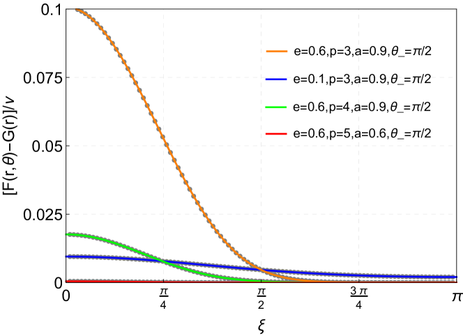
Figure 1: Error of the approximation of the coupling function $F(r,\theta)$. The solid line and points represent $\nu=10^{-4}$ and $10^{-6}$ respectively. It is a very close approximation to substitute the r function $G(r)$ for $F(r,\theta)$. Even if we chose the extreme orbital parameters near LSO(for the orange line, $p_{s}=2.96M$), the error is less than $0.1\nu$.

Now we can obtain the approximate reduced Carter constant $\hat{\mathcal{K}}$ expressed in terms of ($\theta$, $\hat{P_{\theta}}$) same as Eq. (18) and the other expression in terms of ($r$, $\hat{P_{r}}$)

$$\hat{\mathcal{K}}=\frac{\Big{[}a\hat{L_{z}}\!-\!\left(r^{2}+a^{2}\right)\hat{H}_{\rm eff}\Big{]}^{2}}{r^{2}A(u)+a^{2}}-\Delta_{r}\hat{P_{r}}^{2}-r^{2}-2\frac{\widetilde{\omega}_{\rm fd}+ar^{2}\left(A(u)-1\right)}{r^{2}A(u)+a^{2}}\hat{H}_{\rm eff}\hat{L_{z}}\!\!+G(r)\hat{L_{z}}^{2}\,,$$ (24)

By using these constants of motion, the angular momentum $\hat{P_{\theta}}$ and $\hat{P_{r}}$ can be expressed as

$$\hat{P_{\theta}}^{2}=\hat{Q}-\cos^{2}\theta\bigg{[}a^{2}\left(1-\hat{H}_{\rm eff}^{2}\right)+\cfrac{\hat{L_{z}}^{2}}{\sin^{2}\theta}\bigg{]}\,,$$ (25a)

$$\hat{P_{r}}^{2}=\cfrac{\Big{[}a\hat{L_{z}}\!-\!(r^{2}\!+\!a^{2})\hat{H_{\rm eff}}\Big{]}^{2}\!-\!\left(r^{2}A(u)\!+\!a^{2}\right)\bigg{[}r^{2}\!+\!\hat{\mathcal{K}}\!+\!2\cfrac{\widetilde{\omega}_{\rm fd}+ar^{2}\left(A(u)-1\right)}{r^{2}A(u)+a^{2}}\hat{H}_{\rm eff}\hat{L_{z}}\!-\!G(r)\hat{L_{z}}^{2}\bigg{]}}{\left(r^{2}A(u)\!+\!a^{2}\right)^{2}D^{-1}(u)}\,.$$ (25b)

In Eq. (25a), if $\hat{P}_{\theta}=0$, the polar motion is at the turning points $\theta=\theta_{\rm min}$ or $\pi-\theta_{\rm min}$. Then we get the relation between the semi-Carter “constant” and the orbital inclination,

$$\hat{Q}=\cos^{2}\theta_{\rm min}\bigg{[}a^{2}\left(1-\hat{H}_{\rm eff}^{2}\right)+\cfrac{\hat{L_{z}}^{2}}{\sin^{2}\theta_{\rm min}}\bigg{]}\,.$$ (26)

This semi-Carter constant has the same form as in the test-particle case, but with mass-ratio corrections hidden in $H_{\rm eff}$ and $L_{z}$, which will be given explicitly later.

There is another straightforward way to get $\boldmath{P}$ by numerically solving the Hamiltonian equations (10). We then compare the analytical equation Eq. (25a) and the numerical results (also including the spin terms like as $H_{s}$) and show the results in Table 1. We find that our analytical approximations are very close to the numerical results, even for a mass ratio as large as 0.01, which proves that our approximation works well for EMRIs or even intermediatemass-ratio inspirals.

Table 1: Comparison of the maximum $\hat{P_{\theta}}$ ($\hat{P_{\theta}}$ at $\theta=\pi/2$) between the analytical formalism and numerical integration.

$\nu=0.01$	analytical max$\hat{P_{\theta}}$	numerical max$\hat{P_{\theta}}$
$p=8,e=1/3,a=0.99,\theta_{\rm min}=\pi/4$	$2.2909944716$	$2.2909945165$
$p=4,e=1/3,a=0.99,\theta_{\rm min}=\pi/4$	$1.8126129568$	$1.8126323323$
$p=8,e=1/3,a=0.1,\theta_{\rm min}=\pi/4$	$2.5258065572$	$2.5258065544$
$p=8,e=1/3,a=0.99,\theta_{\rm min}=\pi/10$	$3.2445223467$	$3.2445223751$

III.2 Reparametrization of the energy and angular momentum

Solving Eqs. (11) and (13a) for ${H}_{\rm eff}$ yields the effective Hamiltonian associated with the deformed Kerr metric

$${H}_{\rm eff}=\frac{g^{t\phi}}{g^{tt}}P_{\phi}+\frac{1}{\sqrt{-g^{tt}}}\sqrt{\mu^{2}+\Bigg{[}g^{\phi\phi}-\frac{(g^{t\phi})^{2}}{g^{tt}}\Bigg{]}P_{\phi}^{2}+g^{rr}P_{r}^{2}+g^{\theta\theta}P^{2}_{\theta}}\,,$$ (27)

The energy of the system is given by

$$E=H_{\rm EOB},$$ (28)

which implies the relation

$$\hat{H}_{\rm eff}(E)=1+\frac{1}{2\nu}\left(\frac{E^{2}}{M^{2}}-1\right).$$ (29)

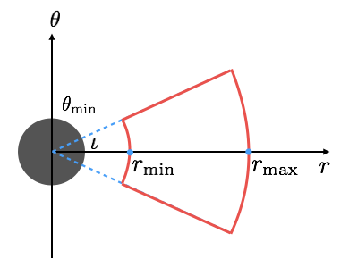
Figure 2: Diagram of 3D motion of a CO around a Kerr black hole. The area encircled by the solid red line is the section of trajectories on the $r$-$\theta$ plane. Here, $r_{\rm max/min}$ is just $r_{1/2}$ in Eq. (30).

The constants of motion and the dynamical equations in the last subsection can be written in terms of the geometrized orbital elements: the semilatus rectum $p$, eccentricity $e$, and orbital inclination $\iota$. This will make the description of the system more intuitive. For an eccentric orbit, there exist apastron and periastron points which can be expressed as

$$r_{1}=\frac{pM}{1-e},\ \ \ \ \ r_{2}=\frac{pM}{1+e},$$ (30)

where $r_{1},r_{2}$ are the turning points of the radial motion. $\theta_{\rm min}$ and $\pi-\theta_{\rm min}$ is the turning points of polar motion, and $\iota\equiv\pi/2-\theta_{\rm min}$ defines the so-called orbital inclination (see Fig. 2). These turning points are computed by solving the radial and polar equations of motion for $\dot{r}=0,\dot{\theta}=0$. By setting the radial and polar equations of motion equals to zero with $P_{r}=P_{\theta}=0$, evaluating Eq. (29) at $(r_{1},\theta_{\rm min})$ and $(r_{2},\theta_{\rm min})$ leads to

$$\hat{L}_{z}^{2}\! =\!\frac{\left(a_{1}\!-\!a_{2}\right)^{2}\left(b_{1}^{2}\!+\!b_{2}^{2}\right)\!-\!(b_{1}^{2}\!-\!b_{2}^{2})(b_{1}^{2}c_{1}\!-\!b_{2}^{2}c_{2})\!-\!2(a_{1}\!-\!a_{2})b_{1}b_{2}\sqrt{\left(a_{1}\!-\!a_{2}\right)^{2}\!-\!\left(b_{1}^{2}\!-\!b_{2}^{2}\right)\left(c_{1}\!-\!c_{2}\right)}}{\left[(a_{1}\!-\!a_{2})^{2}\!-\!\left(b_{1}^{2}c_{1}\!-\!b_{2}^{2}c_{2}\right)\right]^{2}}$$ (31a)

$$\frac{E^{2}}{M^{2}}\! =\!1+2\nu\left(a_{1}\hat{L}_{z}\!+\!\sqrt{\frac{c_{1}\hat{L}_{z}^{2}\!+\!1}{b_{1}}}-1\right)\qquad$$ (31b)

where the coefficients are

$$a_{1} =\frac{\widetilde{\omega}_{\rm fd1}}{\Lambda_{t1}}\,,$$ (32a)

$$a_{2} =\frac{\widetilde{\omega}_{\rm fd2}}{\Lambda_{t2}}\,,$$ (32b)

$$b_{1} =\sqrt{\frac{\Sigma_{1}\Delta_{t1}}{\Lambda_{t1}}}\,,$$ (32c)

$$b_{2} =\sqrt{\frac{\Sigma_{2}\Delta_{t2}}{\Lambda_{t2}}}\,,$$ (32d)

$$c_{1} =\frac{\Sigma_{1}}{\left(1-\cos^{2}\theta_{\rm min}\right)\Lambda_{t1}}\,,$$ (32e)

$$c_{2} =\frac{\Sigma_{2}}{\left(1-\cos^{2}\theta_{\rm min}\right)\Lambda_{t2}},$$ (32f)

in which the subscripts 1 and 2 mean that the function is to be evaluated at $(r_{1},\theta_{\rm min})$ and $(r_{2},\theta_{\rm min})$,

$$\Sigma_{1} =a^{2}\cos^{2}\theta_{\rm min}+r_{1}^{2}\,,$$ (33a)

$$\Sigma_{2} =a^{2}\cos^{2}\theta_{\rm min}+r_{2}^{2}\,,$$ (33b)

$$\Delta_{t1} =a^{2}+A(r_{1})r_{1}^{2}\,,$$ (33c)

$$\Delta_{t2} =a^{2}+A(r_{2})r_{2}^{2}\,,$$ (33d)

$$\Lambda_{t1} =\left(a^{2}+r_{1}^{2}\right)^{2}-a^{2}\sin^{2}\theta_{\rm min}\Delta_{t1}\,,$$ (33e)

$$\Lambda_{t2} =\left(a^{2}+r_{2}^{2}\right)^{2}-a^{2}\sin^{2}\theta_{\rm min}\Delta_{t2}\,,$$ (33f)

$$\widetilde{\omega}_{\rm fd1} =\frac{a^{3}\nu\omega_{2}}{r_{1}}+\frac{a\nu\omega_{1}}{r_{1}}+2ar_{1}\,,$$ (33g)

$$\widetilde{\omega}_{\rm fd2} =\frac{a^{3}\nu\omega_{2}}{r_{2}}+\frac{a\nu\omega_{1}}{r_{2}}+2ar_{2}.$$ (33h)

The above formalism for a Kerr black hole is much more complicated than the Schwarzschild ones in Ref. hinderer2017foundations . Obviously, for the test-particle limit $\nu\to 0$, the above results will go back to the geodesic motion of a test particle in Kerr spacetime.

III.3 Determination of the fundamental frequencies

Since in our approximation the equations of motion in the deformed-Kerr spacetime are separable in the coordinates $r$, $\theta$, and $\phi$, the action variables can be calculated from cyclic integrals over the spatial conjugate momenta in the Boyer-Lindquist coordinate representation:

$$J_{r} =\frac{1}{2\pi}\oint P_{r}\,\mathrm{d}r\,,$$ (34)

$$J_{\theta} =\frac{1}{2\pi}\oint P_{\theta}\,\mathrm{d}\theta\,,$$ (35)

$$J_{\phi} =\frac{1}{2\pi}\oint P_{\phi}\,\mathrm{d}\phi=L_{z}\,.$$ (36)

The standard procedure of determining fundamental frequencies is to find the explicit form of the Hamiltonian in the action-angle representation, $H^{(\mathrm{aa})}$, and calculate the frequencies from the partial derivatives with respect to the radial and polar action variables $J_{k}$ goldstein1980classical :

$$\mu\omega_{k}=\frac{\partial H}{\partial J_{k}}^{(\mathrm{aa})}\,.$$ (37)

Unfortunately, Eqs. (34) and (35) cannot be solved analytically, and so they do not admit an explicit inversion. However, according to the Schmidt method Schmidt2002Celestial , Eq. (37) can be solved even without knowing the functional form of the Hamiltonian $H^{(\mathrm{aa})}$ if the theorem on implicit functions is employed.

Let $P_{\beta}^{(\mathrm{aa})}=f_{\beta}^{(\mathrm{aa})}(-\mu^{2}/2,H_{\rm eff},L_{z},Q)$ be the momenta given by $P_{0}^{(\mathrm{aa})}=p_{t}=-H_{\rm eff}$ and $P_{k}^{(\mathrm{aa})}=J_{k}$. If we denote the Jacobian matrix of $f$ by $\mathsfsl{D}f$, then, by the theorem on implicit functions, $\mathsfsl{D}f\cdot\mathsfsl{D}(f^{-1})=\mathsfsl{D}f\cdot(\mathsfsl{D}f)^{-1}=\mathsfsl{I}$, provided that $f$ is non-zero and the Jacobian does not vanish 1979Analysis . As $-\mu^{2}/2$ is the invariant value of the Hamiltonian, we can substitute $-\mu^{2}/2=g^{\alpha\beta}P_{\alpha}P_{\beta}/2=H^{(\mathrm{aa})}(-H_{\rm eff},J_{k})$. In addition, two rows of the Jacobian matrix are trivial due to the identities $P_{0}^{(\mathrm{aa})}=-H_{\rm eff}$ and $J_{\phi}=L_{z}$. For simplicity, we use the symbol $H$ to denote the Hamiltonian $H^{(\mathrm{aa})}$ below. Thus, the equation $\mathsfsl{D}f\cdot\mathsfsl{D}(f^{-1})=\mathsfsl{I}$ reads

$$\left(\begin{array}[]{llll}0&-1&0&0\\ \frac{\partial J_{r}}{\partial H}&\frac{\partial J_{r}}{\partial H_{\rm eff}}&\frac{\partial J_{r}}{\partial L_{z}}&\frac{\partial J_{r}}{\partial Q}\\ \frac{\partial J_{\theta}}{\partial H}&\frac{\partial J_{\theta}}{\partial H_{\rm eff}}&\frac{\partial J_{\theta}}{\partial L_{z}}&\frac{\partial J_{\theta}}{\partial Q}\\ 0&0&1&0\end{array}\right)\cdot\left(\begin{array}[]{llll}-\frac{\partial H}{\partial H_{\rm eff}}&\frac{\partial H}{\partial J_{r}}&\frac{\partial H}{\partial J_{\theta}}&\frac{\partial H}{\partial J_{\phi}}\\ -1&0&0&0\\ 0&0&0&1\\ -\frac{\partial Q}{\partial H_{\rm eff}}&\frac{\partial Q}{\partial J_{r}}&\frac{\partial Q}{\partial J_{\theta}}&\frac{\partial Q}{\partial J_{\phi}}\\ \end{array}\right)=\mathsfsl{I}.$$ (38)

The above matrix equation is valid if and only if the orbit is nonequatorial Schmidt2002Celestial . We have discussed the condition of equatorial orbits in our previous work zc2020 . Then, it can be split into four nontrivial sets of linear equations in the eight unknowns $-\frac{\partial H}{\partial H_{\rm eff}}$, $\frac{\partial H}{\partial J_{k}}$, $-\frac{\partial Q}{\partial H_{\rm eff}}$, and $\frac{\partial Q}{\partial J_{k}}$:

$$- \mathsfsl{A}\cdot\frac{\partial}{\partial H_{\rm eff}}\left(\begin{array}[]{llll}H\\ Q\end{array}\right)=\left(\begin{array}[]{llll}2W(r_{1},r_{2})\\ 2a^{2}H_{\rm eff}U(\theta_{\rm min},\pi/2)\end{array}\right)$$ (58)

$$\mathsfsl{A}\cdot\frac{\partial}{\partial J_{r}}\left(\begin{array}[]{llll}H\\ Q\end{array}\right)=\left(\begin{array}[]{llll}2\pi\\ 0\end{array}\right),$$

$$\mathsfsl{A}\cdot\frac{\partial}{\partial J_{\theta}}\left(\begin{array}[]{llll}H\\ Q\end{array}\right)=\left(\begin{array}[]{llll}0\\ \pi\end{array}\right),$$

$$\mathsfsl{A}\cdot\frac{\partial}{\partial J_{\phi}}\left(\begin{array}[]{llll}H\\ Q\end{array}\right)=\left(\begin{array}[]{llll}2Z(r_{1},r_{2})\\ 2L_{z}V(\theta_{\rm min},\pi/2)\end{array}\right),$$

with the coefficient matrix

$$\mathsfsl{A}=\left(\begin{array}[]{llll}2\pi\frac{\partial J_{r}}{\partial H}&2\pi\frac{\partial J_{r}}{\partial Q}\\ \pi\frac{\partial J_{\theta}}{\partial H}&\pi\frac{\partial J_{\theta}}{\partial Q}\end{array}\right)=\left(\begin{array}[]{llll}2Y(r_{1},r_{2})&-X(r_{1},r_{2})\\ 2a^{2}U(\theta_{\rm min},\pi/2)&T(\theta_{\rm min},\pi/2)\end{array}\right),$$ (59)

where $r_{1}$ and $r_{2}$ are the turning points of radial motion, and $X(r_{1},r_{2})$, $Y(r_{1},r_{2})$,$Z(r_{1},r_{2})$ and $W(r_{1},r_{2})$ are radial integrals defined by

$$X(r_{1},r_{2}) = \int_{r_{1}}^{r_{2}}\frac{\mathrm{d}r}{\Delta_{r}P_{r}},$$ (60a)

$$Y(r_{1},r_{2}) = \int_{r_{1}}^{r_{2}}\frac{r^{2}\,\mathrm{d}r}{\Delta_{r}P_{r}},$$ (60b)

$$Z(r_{1},r_{2}) =- \int_{r_{1}}^{r_{2}}\frac{\partial P_{r}}{\partial L_{z}}\,\mathrm{d}r,$$ (60c)

$$W(r_{1},r_{2}) = \int_{r_{1}}^{r_{2}}\frac{\partial P_{r}}{\partial H_{\rm eff}}\,\mathrm{d}r,$$ (60d)

$T(\theta_{\rm min},\pi/2)$, $U(\theta_{\rm min},\pi/2)$, and $V(\theta_{\rm min},\pi/2)$ are polar integrals defined by

$$T(\theta_{\rm min},\pi/2) = \int_{\theta_{\rm min}}^{\pi/2}\frac{\mathrm{d}\theta}{P_{\theta}},$$ (61a)

$$U(\theta_{\rm min},\pi/2) = \int_{\theta_{\rm min}}^{\pi/2}\frac{\cos^{2}\theta}{P_{\theta}}\,\mathrm{d}\theta,$$ (61b)

$$V(\theta_{\rm min},\pi/2) = \int_{\theta_{\rm min}}^{\pi/2}\frac{\cot^{2}\theta}{P_{\theta}}\,\mathrm{d}\theta.$$ (61c)

The above radial functions $X,Y,Z,W$ and polar functions $T,U,V$ are not proper integrals because the integrated functions are divergent at the turning points $r_{1},r_{2}$ and $\theta_{\rm min},\pi-\theta_{\rm min}$. Thus, we define $\xi$ by the equation $r=pM/(1+e\cos\xi)$, where $p$ is called the semi-latus rectum and $e$ is the eccentricity of the orbit, and we define $\chi$ with $\cos^{2}\theta=\cos^{2}\theta_{\rm min}\cos^{2}\chi$. As $\xi$ varies from $0$ to $2\pi$ as $r$ goes through a complete cycle, $\chi$ varies from $0$ to $2\pi$ as $\theta$ oscillates through its full range of motion. Then transform $X,Y,X,W$ and $T,U,V$ into well-behaved integrals

$$X = \int_{0}^{\pi}\frac{ep\sin\xi}{(1+e\cos\xi)^{2}}\frac{\mathrm{d}\xi}{\Delta_{r}P_{r}},$$ (62a)

$$Y = \int_{0}^{\pi}\frac{ep\sin\xi}{(1+e\cos\xi)^{2}}\frac{r^{2}\,\mathrm{d}\xi}{\Delta_{r}P_{r}},$$ (62b)

$$Z =- \int_{0}^{\pi}\frac{ep\sin\xi}{(1+e\cos\xi)^{2}}\frac{\partial P_{r}}{\partial L_{z}}\,\mathrm{d}\xi,$$ (62c)

$$W = \int_{0}^{\pi}\frac{ep\sin\xi}{(1+e\cos\xi)^{2}}\frac{\partial P_{r}}{\partial H_{\rm eff}}\,\mathrm{d}\xi,$$ (62d)

which transforming Eq. (25a) to

$$\beta^{2}(z^{2}-z_{+}^{2})(z^{2}-z_{-}^{2})=P_{\theta}^{2}(1-z^{2})\,,$$ (63)

where $\beta^{2}=a^{2}(\mu^{2}-{H_{\rm eff}}^{2})$, $z_{\pm}^{2}$ are the two roots of the equation $P_{\theta}=0$ when substituting $\cos\theta=z$ in $P_{\theta}$ and given by

$$z_{-} = \cos\theta_{\rm min}\,,$$ (64)

$$z_{+} = \cfrac{L_{z}^{2}+Q+\beta+\sqrt{(L_{z}^{2}+Q+\beta)^{2}-4\beta Q}}{2\beta}\,,$$ (65)

by this way, Schmidt derives the following expressions Schmidt2002Celestial for the polar integrals

$$T = \frac{1}{\beta z_{+}}K(k)\,,$$ (66a)

$$U = \frac{z_{+}}{\beta}[K(k)-E(k)]\,,$$ (66b)

$$V = \frac{z_{+}}{\beta}[\Pi(z_{-}^{2},k)-K(k)]\,,$$ (66c)

where $k=z_{-}^{2}/z_{+}^{2}$, $K(k)$, $E(k)$ and $\Pi(z_{-}^{2},k)$ are, respectively, the complete elliptical integrals of the first, second and third kind,

$$K(k) = \int_{0}^{\pi/2}\!\frac{\mathrm{d}\chi}{\sqrt{1-k\sin^{2}\chi}},$$ (67a)

$$E(k) = \int_{0}^{\pi/2}\!\sqrt{1-k\sin^{2}\chi}\,\mathrm{d}\chi,$$ (67b)

$$\Pi({z_{-}^{2},k}) = \int_{0}^{\pi/2}\!\frac{\mathrm{d}\chi}{\left(1-z_{-}^{2}\sin^{2}\chi\right)\sqrt{1-k\sin^{2}\chi}},$$ (67c)

The solutions of the above systems of equations for $-\frac{\partial H}{\partial H_{\rm eff}}$ and $\frac{\partial H}{\partial J_{k}}$ are given by

$$- \frac{\partial H}{\partial H_{\rm eff}}=\frac{K(k)W+a^{2}z_{+}^{2}E\left[K(k)-E(k)\right]X}{K(k)Y+a^{2}z_{+}^{2}\left[K(k)-E(k)\right]X},$$ (71)

$$\frac{\partial H}{\partial J_{r}}=\frac{\pi K(k)}{K(k)Y+a^{2}z_{+}^{2}\left[K(k)-E(k)\right]X},$$

$$\frac{\partial H}{\partial J_{\theta}}=\frac{\pi\beta z_{+}X}{2\{K(k)Y+a^{2}z_{+}^{2}\left[K(k)-E(k)\right]X\}},$$

$$\frac{\partial H}{\partial J_{\phi}}=\frac{K(k)Z+L_{z}[\Pi(z_{-}^{2},k)-K(k)]X}{K(k)Y+a^{2}z_{+}^{2}[K(k)-E(k)]X}.$$

From Eqs. (37) and (71)-(71), the coordinate-time frequencies $\omega_{r},\omega_{\theta}$ and $\omega_{\phi}$ are obtained

$$\omega_{r} =\frac{\pi K(k)}{K(k)W+a^{2}z_{+}^{2}E\left[K(k)-E(k)\right]X},$$ (72)

$$\omega_{\theta} =\frac{\pi\beta z_{+}X}{2\{K(k)W+a^{2}z_{+}^{2}E\left[K(k)-E(k)\right]X\}},$$ (73)

$$\omega_{\phi} =\frac{K(k)Z+L_{z}[\Pi(z_{-}^{2},k)-K(k)]X}{K(k)W+a^{2}z_{+}^{2}E\left[K(k)-E(k)\right]X}.$$ (74)

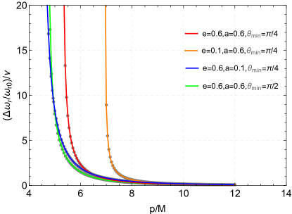
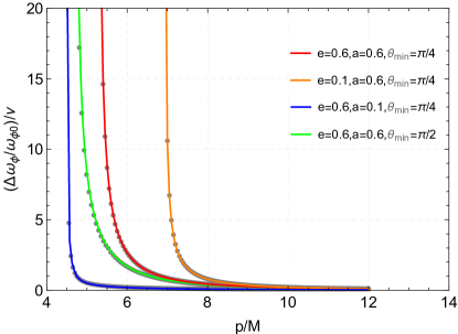
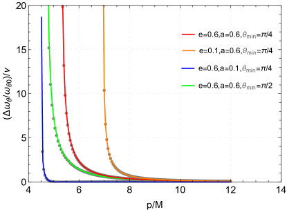
Figure 3: Frequency shifts $\frac{\Delta\omega}{\nu\omega_{0}}$ vs semilatus rectum $p$ in the cases of various $a,~{}\nu,~{}e,~{}\theta_{\rm min}$. The solid line and points represent $\nu=10^{-4}$ and $10^{-6}$ respectively.

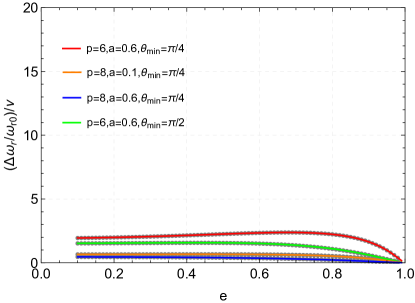
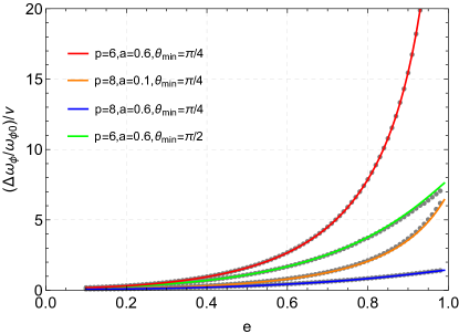
Figure 4: Frequency shifts $\frac{\Delta\omega}{\nu\omega_{0}}$ vs eccentricity $e$ in the cases of various $a,~{}\nu,~{}p,~{}\theta_{\rm min}$. The solid line and points represent $\nu=10^{-4}$ and $10^{-6}$ respectively.

Figure 5: Frequency shifts $\frac{\Delta\omega}{\nu\omega_{0}}$ vs the minimal polar angle $\theta_{\rm min}$ in the cases of various $a,~{}\nu,~{}p,~{}e$. The solid line and points represent $\nu=10^{-4}$ and $10^{-6}$ respectively.

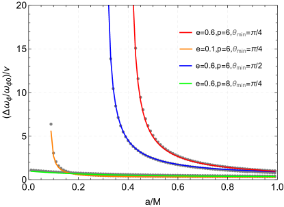
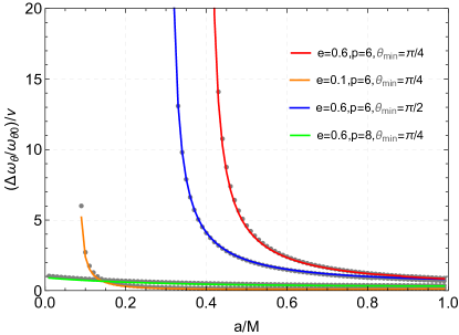
Figure 6: Frequency shifts $\frac{\Delta\omega}{\nu\omega_{0}}$ vs spin $a$ in the cases of various $~{}\nu,~{}p,~{}e,~{}\theta_{\rm min}$. The solid line and points represent $\nu=10^{-4}$ and $10^{-6}$ respectively.

The above equations have the same forms as the test particle ones given in Schmidt2002Celestial . However, the mass-ratio corrections have to be encoded in each variable. To explore the influence of the mass ratio on these frequencies, we demonstrate the relative frequency shift $(\omega(\nu)-\omega_{0})/\omega_{0}$ (where the subscript 0 means the test-particle case $\nu\rightarrow 0$) with varied orbital parameters.

In Fig. 3, we can see that the three frequency shifts due to the mass ratio corrections are one order larger than the mass-ratio, especially when $p$ approaches $p_{s}$ (the edge of last stable orbit). The effective spin terms we omitted at the beginning of this section have much smaller magnitudes. This proves again that the approximation we made is reasonable for EMRIs.

Fig. 4 demonstrates the relations of frequency shifts due to mass ratios with eccentricities. Interestingly, the azimuthal and polar frequency shifts increase when the eccentricity grows, but the radial frequency error is not sensitive to the eccentricity [about $O(\nu)$]. When $e$ becomes extreme, the shift decreases.

The variation of frequency shifts also depends on the orbital inclination. In Fig. 5, for the small semilatus rectum, the frequency errors due to mass ratio grow very fast when the orbital inclination $\iota$ increases (i.e., $\theta_{\rm min}\rightarrow 0$). However, for large $p$, the frequency shifts are not very sensitive to the orbital inclination.

Finally, Fig. 6 shows the frequency shifts vs the effective Kerr parameter $a$ (approachs to the Kerr parameter of the central black hole when $\nu\rightarrow 0$). When $a$ becomes smaller, the last stable orbit (LSO) is farther away from the black hole (i.e., $p_{s}$ becomes larger). Then for the fixed $p=6$, the orbit is closer to the LSO as $a$ decreases, so we can see that the frequency shifts increase. When $p=8$, which is just a little larger than the radius of the innermost stable circular orbit ($r_{\rm isco}=6$ for a nonspinning BH), the dependence is no longer obvious

All of the above results state that the mass-ratio correction has a substantial influence on the orbital frequencies even for the extreme-mass-ratio limit. This means that in the construction of the waveform templates for EMRIs, the mass ratio needs to be included in the orbital calculations. However, as we stated in the Introduction, the frequency shifts in Fig. 3-6 are not guaranteed quantitatively. Comparison of innermost stable circular orbit (ISCO) shifts between the EOB and gravitational self-force (GSF) in Isoyama2014 shows obvious deviation, but still hints that the frequency shift is at about the same order of mass ratio, which coincides with our results in Fig. 3-6. The ISCO shifts in Isoyama2014 were calculated based on an earlier version of the EOB potential; we recalculated the ISCO shifts based on the updated potential which is used in this work steinhoff2016Apotential , and we found that the results improve a lot (see Fig. 7). If the spin of a SMBH is not extreme (below 0.8 based on the Fig. 7), the EOB’s ISCO frequency shifts exhibit less than a 50support our results in Figs. 3-6 which qualitatively state that the influence of the mass ratio on the conservative dynamics of EMRIs cannot be ignored and give qualitative magnitudes. In other words, the test-particle approximation may not be enough for the EMRI waveform simulation, and we expect more accurate self-force corrections.

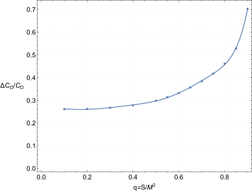
Figure 7: Relative difference of ISCO frequency shift $\Delta C_{\Omega}/C_{\Omega}:=1-C^{EOB}_{\Omega}/C_{\Omega}^{GSF}$ between the EOB and GSF methods Isoyama2014 .

III.4 Orbits of conservative dynamics

We find evolution equations for $r$, $\phi$, and $\chi$ with the forms

$$\dot{r} =\frac{\partial E}{\partial P_{r}}\!=\!-\frac{g^{rr}\hat{P_{r}}}{E/M\left(g^{tt}\hat{H}_{\rm eff}-g^{t\phi}\hat{L}_{z}\right)}\,,$$ (75a)

$$\dot{\phi} =\frac{\partial E}{\partial P_{\phi}}\!=\!\frac{g^{t\phi}-\Big{[}g^{tt}g^{\phi\phi}-(g^{t\phi})^{2}\Big{]}\frac{\hat{L}_{z}}{g^{tt}\hat{H}_{\rm eff}-g^{t\phi}\hat{L}_{z}}}{g^{tt}E/M}\,,$$ (75b)

$$\dot{\theta}\! =\frac{\partial E}{\partial P_{\theta}}\!=\!-\frac{g^{\theta\theta}\hat{P_{\theta}}}{E/M\left(g^{tt}\hat{H}_{\rm eff}-g^{t\phi}\hat{L}_{z}\right)}\,.$$ (75c)

where $\hat{P}_{r}$, $\hat{P}_{\theta}$ have been analytically obtained in Eqs. (25a)-(25b), and $\hat{H}_{\rm eff}$, $\hat{L}_{z}$ have been given in Eq. (31). The metric components are Eqs. (3a)-(3e). Due to the definitions of $\xi,~{}\chi$, all the variables by $r$ and $\theta$ can be transfer to the functions of $\xi,~{}\chi$. Finally, the above equations can now be expressed in terms of only the variables $(\xi,\chi)$ and orbital parameters $(p,e,\theta_{\rm min})$ or $(p,e,\iota)$,

$$\dot{\xi} =-\frac{(1+e\cos\xi)^{2}}{epM\sin\xi}\frac{g^{rr}\hat{P_{r}}}{E/M\left(g^{tt}\hat{H}_{\rm eff}-g^{t\phi}\hat{L}_{z}\right)}=\Xi(p,e,\iota,\xi,\chi)\,,$$ (76a)

$$\dot{\chi}\! =-\frac{g^{\theta\theta}\sqrt{\left(a^{2}\left(1-\hat{H}_{\rm eff}^{2}\right)\right)\left(z_{+}^{2}-z_{-}^{2}\cos^{2}\chi\right)}}{E/M\left(g^{tt}\hat{H}_{\rm eff}-g^{t\phi}\hat{L}_{z}\right)}=\Theta(p,e,\iota,\xi,\chi)\,,$$ (76b)

$$\dot{\phi} =\frac{g^{t\phi}-\Big{[}g^{tt}g^{\phi\phi}-(g^{t\phi})^{2}\Big{]}\frac{\hat{L}_{z}}{g^{tt}\hat{H}_{\rm eff}-g^{t\phi}\hat{L}_{z}}}{g^{tt}E/M}=\Phi(p,e,\iota,\xi,\chi)\,.$$ (76c)

The detailed expressions of $\Xi,\Theta$ and $\Phi$ can be directly obtained, but they are too long to be written here. Solving the above ordinary differential equations by numerical integration, we can get $\xi$, $\chi$, and $\phi$ associated with coordinate time $t$, i.e., the orbital motion. Projecting the Boyer-Lindquist coordinates onto a spherical coordinate grid, we can define the corresponding Cartesian coordinate system,

$$\tilde{x} = \cfrac{p\cos\phi\sqrt{1-z_{-}^{2}\cos^{2}\chi}}{1+e\cos\xi}\,,$$ (77a)

$$\tilde{y} = \cfrac{p\sin\phi\sqrt{1-z_{-}^{2}\cos^{2}\chi}}{1+e\cos\xi}\,,$$ (77b)

$$\tilde{z} = \cfrac{pz_{-}\cos\chi}{1+e\cos\xi}\,.$$ (77c)

Combining the equations of the motion (76a) - (76c) we can plot the orbits of conservative dynamics in the Cartesian coordinates (see Fig. 8).

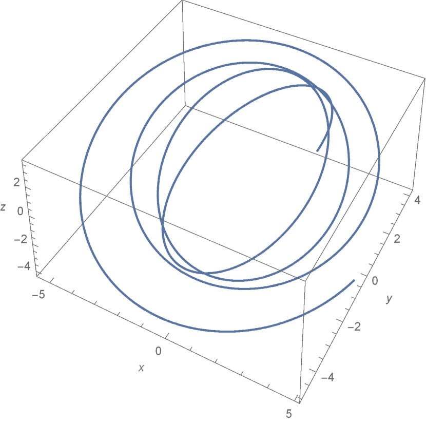
(a)  $a=0.5~{}M,\;e=0.2,\;p=5~{}M,\;p_{s}=4.99~{}M$

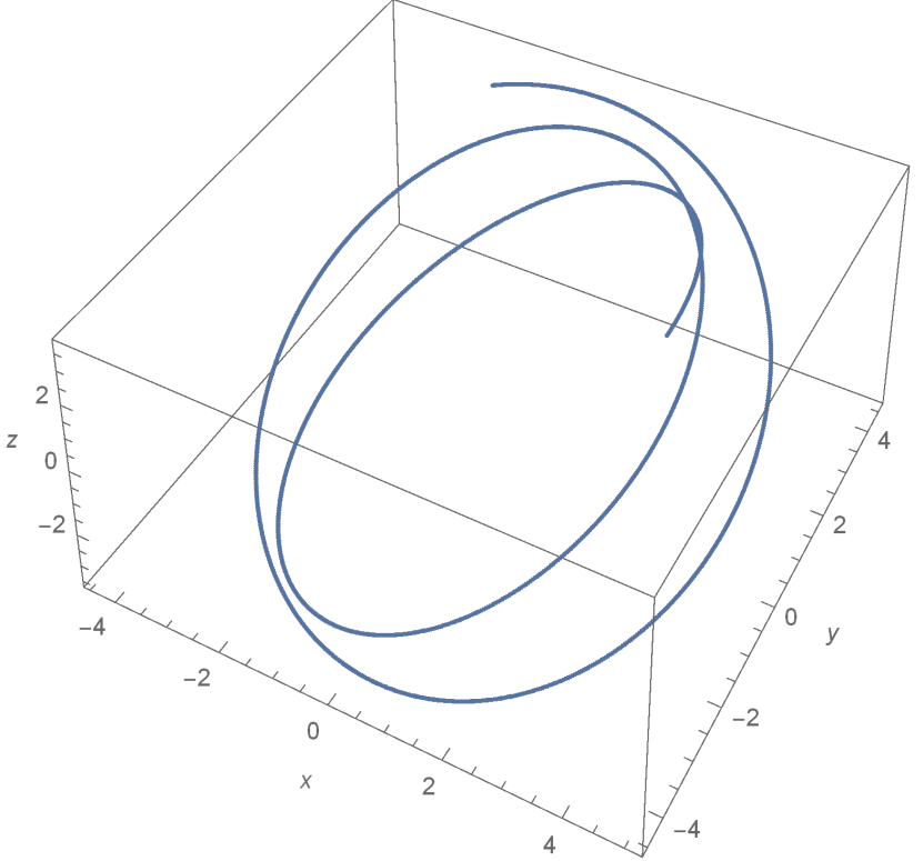
(b)  $a=0.5~{}M,\;e=0.1,\;p=5~{}M,\;p_{s}=4.84~{}M$

(c)  $a=0.6~{}M,\;e=0.6,\;p=6~{}M,\;p_{s}=5.28~{}M$

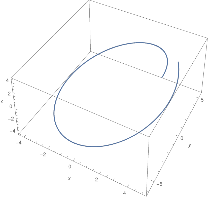
(d)  $a=0.6~{}M,\;e=0.1,\;p=6~{}M,\;p_{s}=4.51~{}M$

Figure 8: Four orbits of different initial parameters. We set $\nu=10^{-4},\theta_{\rm min}=\pi/4$ in the all four orbits and just plot half orbital period from the apastron to the periastron.

Like the zoom-whirl orbits glampedakis2002zoom in $r$-$\phi$ components, from Fig. 8 there are similar zoom-whirl phenomena in the $r$-$\theta$ directions. Different orbital parameters with a corresponding prograde separatrix have different polar angular periods. We can imagine that as the orbit gradually approaches the separatrix, the test particle will spend a more considerable amount of its orbital “life” (in both the azimuthal and polar directions) close to the periastron.

III.5 Evolution of orbital parameters under radiation reaction

The description of geodesic motion around BHs is based on the semilatus rectum $p$, the eccentricity $e$ and the orbital inclination $\iota$, together with three phase variables associated with the spatial geometry of the radial, azimuthal and polar motion denoted by $(\xi,\phi,\chi)$. $\xi$ was already defined by expressing the radial motion as

$$r=\frac{pM}{1+e\cos\xi}\,.\\$$ (78)

Taking the derivation of Eq. (78), we get the evolution equation for the phase variable $\xi$,

$$\dot{\xi}=\frac{(1+e\cos\xi)^{2}}{epM\sin\xi}\dot{r}-\frac{1+e\cos\xi}{ep\sin\xi}\dot{p}+\frac{\cot\xi}{e}\dot{e}.$$ (79)

For a conservative system, $\dot{p}=\dot{e}=0$. However, if we take the radiation reaction of GWs into account, the rate of change of the energy, the reduced angular momentum, and the Carter constant are given by

$$\frac{dE}{dt} =\frac{\partial E}{\partial p}\dot{p}+\frac{\partial E}{\partial e}\dot{e}+\frac{\partial E}{\partial\iota}\dot{\iota}\,,$$ (80a)

$$\frac{d\hat{L}_{z}}{dt} =\frac{\partial\hat{L}_{z}}{\partial p}\dot{p}+\frac{\partial\hat{L}_{z}}{\partial e}\dot{e}+\frac{\partial\hat{L}_{z}}{\partial\iota}\dot{\iota}\,,$$ (80b)

$$\frac{d\hat{Q}}{dt} =\frac{\partial\hat{Q}}{\partial p}\dot{p}+\frac{\partial\hat{Q}}{\partial e}\dot{e}+\frac{\partial\hat{Q}}{\partial\iota}\dot{\iota}\,.$$ (80c)

From Eqs. (80a)-(80c), we express the evolution of $(p,~{}e,~{}\iota)$ using the energy and angular momentum fluxes of gravitational radiation,

$$\dot{p} =c_{(\hat{L}_{z},\hat{Q})(e,\iota)}\frac{dE}{dt}+c_{(E,\hat{Q})(\iota,e)}\frac{d\hat{L}_{z}}{dt}+c_{(E,\hat{L}_{z})(e,\iota)}\frac{d\hat{Q}}{dt}\,$$ (81a)

$$\dot{e} =c_{(\hat{L}_{z},\hat{Q})(\iota,p)}\frac{dE}{dt}+c_{(E,\hat{Q})(p,\iota)}\frac{d\hat{L}_{z}}{dt}+c_{(E,\hat{L}_{z})(\iota,p)}\frac{d\hat{Q}}{dt}\,$$ (81b)

$$\dot{\iota} =c_{(\hat{L}_{z},\hat{Q})(p,e)}\frac{dE}{dt}+c_{(E,\hat{Q})(e,p)}\frac{d\hat{L}_{z}}{dt}+c_{(E,\hat{L}_{z})(p,e)}\frac{d\hat{Q}}{dt},$$ (81c)

where the coefficients are given by

$$c_{(C_{1},C_{2})(o_{1},o_{2})}=\frac{\Big{[}\frac{\partial C_{1}}{\partial o_{1}}\frac{\partial C_{2}}{\partial o_{2}}-\frac{\partial C_{1}}{\partial o_{2}}\frac{\partial C_{2}}{\partial o_{1}}\Big{]}}{\Big{[}\frac{\partial E}{\partial\iota}\frac{\hat{L}_{z}}{\partial p}-\frac{\partial E}{\partial p}\frac{\partial\hat{L}_{z}}{\partial\iota}\Big{]}\frac{\partial\hat{Q}}{\partial e}+\Big{[}\frac{\partial E}{\partial e}\frac{\hat{L}_{z}}{\partial\iota}-\frac{\partial E}{\partial\iota}\frac{\partial\hat{L}_{z}}{\partial e}\Big{]}\frac{\partial\hat{Q}_{\phi}}{\partial p}+\Big{[}\frac{\partial E}{\partial p}\frac{\hat{L}_{z}}{\partial e}-\frac{\partial E}{\partial e}\frac{\partial\hat{L}_{z}}{\partial p}\Big{]}\frac{\partial\hat{Q}_{\phi}}{\partial\iota}}\,,\\$$ (81d)

where $C=\{E,\hat{L}_{z},\hat{Q}\}$ and $o=\{p,e,\iota\}$, and the derivatives can be computed from the expressions in Eqs. (26) and (31). We do not write the complete expressions here because they can be calculated quite directly but are very long.

Once we have the GW fluxes $\dot{E},~{}\dot{L}_{z}$, and $\dot{Q}$, the orbital evolution can be obtained. We have no plan to introduce the detailed fluxes in the present paper, and thus we do not calculate the specific orbital evolution here. We will leave this task to the next paper on gravitational waveforms. In this work, we just focus on the geometrization of the EOB formalism in extreme-mass-ratio cases.

The final set of EOB equations of motion with radiation reaction are Eqs.(81a)-(81b) together with the evolution of the phases described by Eqs. (79) and (81c), and the radius of motion at any arbitrary moment is given by Eq. (75a). Now all the equations of motion are expressed in terms of only the geometric parameters $(p,e,\iota,\xi,\chi)$ and the effective Kerr parameter $a$.

IV Conclusions and Outlook

In the present paper, based on the EOB deformed metric and Hamiltonian, we gave the geometrized formalism of the equations of motion for the inclined-eccentric EMRIs with spinning black holes. The solutions were derived with the geometric parameters $p$, $e$ and $\iota$ instead of the EOB coordinates and momentum. The fundamental properties of the motion due to the mass ratio and black hole spin were discussed. We also gave expressions for three orbital frequencies $\omega_{r},~{}\omega_{\theta},~{}\omega_{\phi}$. With these formalisms in hand, it is convenient to obtain the motion of a compact object around a supermassive black hole with the orbital parameters $p,e,\iota$.

Our results show that the influence on the orbital motion due to the small compact object’s gravitational self-force on the background of a SMBH cannot be ignored. The analytical formalism in this work makes the inclusion of the mass ratio in the motion much more intuitive. Though we do not give a waveform template in the present work, We believe that our analytical method (not the formalism themselves) should be an useful way to build waveform models in the future for EMRIs to replace the test-particle approximation which is used in popular waveform models.

In the present work, a few approximations have been used. As we mentioned before, in the present model we temporarily omitted the effective spin of the small object. In the EOB theory, this spin of the effective test particle is $\sim\mu a/M$ even if the small object does not rotate. The omission of this term will only induce a relative error of the Hamiltonian at least two orders lower than the mass ratio. Furthermore, for decoupling the equations of motion, we used the approximation $F(r,\theta)\approx F(r)$. This usually induces an error at $O(10^{-2})\nu$ order, even at the edge of the LSO, the error still $\lesssim 0.1\nu$. The analysis of these approximations performed here showed that the errors could be ignored for EMRIs due to the very small mass ratio (see Table I). By encoding the mass-ratio correction in the Hamiltonian $H_{\rm NS}$, our expressions may be an improvement compared to the test-particle approximation.

However, as stated in the previous sections, the EOB’s description at the extreme-mass-ratio limit does not get guarantee. Considering the comparison of the ISCO shifts with the gravitational self-force has obvious deviation for the extreme spin cases, we can only state our detailed results qualitatively reveal the influences of mass-ratio on the conservative dynamics. Fortunately, our analytical technology presented in this paper can be used to any similar deformed Kerr metrics. Once there is an updated version of the EOB resummation approximation, then the EOB corrections at the extreme-mass-ratio limit are improved or guaranteed, our results can be easily updated too by replacing the EOB potentials, and then we can get an accurate analytical formalism with mass-ratio corrections for the EMRIs.

One of the scientific targets of EMRIs is to detect the spacetime geometry of a SMBH. For this target, an accurate and efficient waveform template is needed. However, this is still a challenge. The analytical orbital solution including the mass ratio, eccentricity, and orbital inclination given in this paper is more accurate than the test-particle model and more convenient than the original EOB equations for inclined-eccentric orbits over a long-term evolution.

Due to the analytical frequencies, a combination with the frequency-domain Teukolsky equation Teukolsky will be more convenient and can generate numerical waveforms. In the future, we will use the formalisms in this work to generate the orbital evolution and waveforms for EMRIs.

References

• [1] K. Danzman et al. Lisa-Laser Interferometer Space Antenna, Pre-Phase A Report. Max-Planck-Institute fur Quantenoptic, Report MPQ 233, 1998.
• [2] Wen-Rui Hu and Yue-Liang Wu. The taiji program in space for gravitational wave physics and the nature of gravity, 2017.
• [3] Jun Luo, Li-Sheng Chen, Hui-Zong Duan, Yun-Gui Gong, Shoucun Hu, Jianghui Ji, Qi Liu, Jianwei Mei, Vadim Milyukov, Mikhail Sazhin, et al. Tianqin: a space-borne gravitational wave detector. Classical and Quantum Gravity, 33(3):035010, 2016.
• [4] Pau Amaro-Seoane, Jonathan R Gair, Marc Freitag, M Coleman Miller, Ilya Mandel, Curt J Cutler, and Stanislav Babak. Intermediate and extreme mass-ratio inspirals—astrophysics, science applications and detection using lisa. Classical and Quantum Gravity, 24(17):R113, 2007.
• [5] Stanislav Babak, Jonathan Gair, Alberto Sesana, Enrico Barausse, Carlos F Sopuerta, Christopher PL Berry, Emanuele Berti, Pau Amaro-Seoane, Antoine Petiteau, and Antoine Klein. Science with the space-based interferometer lisa. v. extreme mass-ratio inspirals. Physical Review D, 95(10):103012, 2017.
• [6] Christopher PL Berry, Scott A Hughes, Carlos F Sopuerta, Alvin JK Chua, Anna Heffernan, Kelly Holley-Bockelmann, Deyan P Mihaylov, M Coleman Miller, and Alberto Sesana. The unique potential of extreme mass-ratio inspirals for gravitational-wave astronomy. arXiv preprint arXiv:1903.03686, 2019.
• [7] Jonathan R Gair, Michele Vallisneri, Shane L Larson, and John G Baker. Testing general relativity with low-frequency, space-based gravitational-wave detectors. Living Reviews in Relativity, 16(1):7, 2013.
• [8] Saul A Teukolsky. Perturbations of a rotating black hole. I. fundamental equations for gravitational electromagnetic and neutrino field perturbations. Astrophys. J., 185:635–647, 1973.
• [9] Leor Barack and Curt Cutler. Lisa capture sources: Approximate waveforms, signal-to-noise ratios, and parameter estimation accuracy. Physical Review D, 69(8):082005, 2004.
• [10] Stanislav Babak, Hua Fang, Jonathan R Gair, Kostas Glampedakis, and Scott A Hughes. “kludge” gravitational waveforms for a test-body orbiting a kerr black hole. Physical Review D, 75(2):024005, 2007.
• [11] Alvin JK Chua, Christopher J Moore, and Jonathan R Gair. Augmented kludge waveforms for detecting extreme-mass-ratio inspirals. Physical Review D, 96(4):044005, 2017.
• [12] Nicolas Yunes, Alessandra Buonanno, Scott A Hughes, M Coleman Miller, and Yi Pan. Modeling extreme mass ratio inspirals within the effective-one-body approach. Physical review letters, 104(9):091102, 2010.
• [13] Nicolas Yunes, Alessandra Buonanno, Scott A Hughes, Yi Pan, Enrico Barausse, M Coleman Miller, and William Throwe. Extreme mass-ratio inspirals in the effective-one-body approach: Quasicircular, equatorial orbits around a spinning black hole. Physical Review D, 83(4):044044, 2011.
• [14] Wen-Biao Han and Zhoujian Cao. Constructing effective one-body dynamics with numerical energy flux for intermediate-mass-ratio inspirals. Physical Review D, 84(4):044014, 2011.
• [15] Wen-Biao Han. Gravitational waves from extreme-mass-ratio inspirals in equatorially eccentric orbits. International Journal of Modern Physics D, 23(07):1450064, 2014.
• [16] Shuo Xin, Wen-Biao Han, and Shu-Cheng Yang. Gravitational waves from extreme-mass-ratio inspirals using general parametrized metrics. Physical Review D, 100(8):084055, 2019.
• [17] Leor Barack and Adam Pound. Self-force and radiation reaction in general relativity. Reports on Progress in Physics, 82(1):016904, 2018.
• [18] Scott A. Hughes Adiabatic and post-adiabatic approaches to extreme mass ratio inspiral. World Scientific, 185:1953–1959, 2018.
• [19] Alessandra Buonanno and Thibault Damour. Effective one-body approach to general relativistic two-body dynamics. Physical Review D, 59(8):084006, 1999.
• [20] Alessandra Buonanno and Thibault Damour. Transition from inspiral to plunge in binary black hole coalescences. Physical Review D, 62(6):064015, 2000.
• [21] Andrea Taracchini, Alessandra Buonanno, Yi Pan, Tanja Hinderer, Michael Boyle, Daniel A Hemberger, Lawrence E Kidder, Geoffrey Lovelace, Abdul H Mroué, Harald P Pfeiffer, et al. Effective-one-body model for black-hole binaries with generic mass ratios and spins. Physical Review D, 89(6):061502, 2014.
• [22] Alessandra Buonanno, Yi Pan, John G Baker, Joan Centrella, Bernard J Kelly, Sean T McWilliams, and James R van Meter. Approaching faithful templates for nonspinning binary black holes using the effective-one-body approach. Physical Review D, 76(10):104049, 2007.
• [23] Michael Pürrer. Frequency domain reduced order model of aligned-spin effective-one-body waveforms with generic mass ratios and spins. Physical Review D, 93(6):064041, 2016.
• [24] Sascha Husa, Sebastian Khan, Mark Hannam, Michael Pürrer, Frank Ohme, Xisco Jiménez Forteza, and Alejandro Bohé. Frequency-domain gravitational waves from nonprecessing black-hole binaries. i. new numerical waveforms and anatomy of the signal. Physical Review D, 93(4):044006, 2016.
• [25] Sebastian Khan, Sascha Husa, Mark Hannam, Frank Ohme, Michael Pürrer, Xisco Jiménez Forteza, and Alejandro Bohé. Frequency-domain gravitational waves from nonprecessing black-hole binaries. ii. a phenomenological model for the advanced detector era. Physical Review D, 93(4):044007, 2016.
• [26] Tony Chu, Heather Fong, Prayush Kumar, Harald P Pfeiffer, Michael Boyle, Daniel A Hemberger, Lawrence E Kidder, Mark A Scheel, and Bela Szilagyi. On the accuracy and precision of numerical waveforms: Effect of waveform extraction methodology. Classical and Quantum Gravity, 33(16):165001, 2016.
• [27] Prayush Kumar, Tony Chu, Heather Fong, Harald P Pfeiffer, Michael Boyle, Daniel A Hemberger, Lawrence E Kidder, Mark A Scheel, and Bela Szilagyi. Accuracy of binary black hole waveform models for aligned-spin binaries. Physical Review D, 93(10):104050, 2016.
• [28] Yi Pan, Alessandra Buonanno, Andrea Taracchini, Lawrence E Kidder, Abdul H Mroué, Harald P Pfeiffer, Mark A Scheel, and Béla Szilágyi. Inspiral-merger-ringdown waveforms of spinning, precessing black-hole binaries in the effective-one-body formalism. Physical Review D, 89(8):084006, 2014.
• [29] Zhoujian Cao and Wen-Biao Han. Waveform model for an eccentric binary black hole based on the effective-one-body-numerical-relativity formalism. Physical Review D, 96(4):044028, 2017.
• [30] Tanja Hinderer and Stanislav Babak. Foundations of an effective-one-body model for coalescing binaries on eccentric orbits. Physical Review D, 96(10):104048, 2017.
• [31] Wen-Biao Han Chen Zhang and Shu-Cheng Yang. Analytical effective-one-body formalism for extreme-mass-ratio inspirals: eccentric orbits. arXiv preprint arXiv:2001.06763, 2021.
• [32] Simone Albanesi, Alessandro Nagar and Sebastiano Bernuzzi. Effective one-body model for extreme-mass-ratio spinning binaries on eccentric equatorial orbits: testing radiation reaction and waveform. arXiv preprint arXiv:2104.10559, 2021.
• [33] A. Nagar, T. Damour, and A. Tartaglia. Binary black hole merger in the extreme-mass-ratio limit. Class. Quant. Grav., 24:S109, 2021.
• [34] T. Damour and A. Nagar. Faithful Effective-One-Body waveforms of small-mass-ratio coalescing black-hole binaries. Physical Review D, 76(6):064028, 2007.
• [35] S. Bernuzzi and A. Nagar. Binary black hole merger in the extreme-mass-ratio limit: A multipolar analysis. Physical Review D, 81(8):084056, 2010.
• [36] S. Bernuzzi, A. Nagar, and A. Zenginoǧlu. Binary black hole coalescence in the extreme-mass-ratio limit: Testing and improving the effective-one-body multipolar waveform. Physical Review D, 83(6):064010, 2011.
• [37] S. Bernuzzi, A. Nagar, and A. Zenginoǧlu. Binary black hole coalescence in the large-mass-ratio limit: The hyperboloidal layer method and waveforms at null infinity. Physical Review D, 84(8):084026, 2011.
• [38] S. Bernuzzi, A. Nagar, and A. Zenginoǧlu. Horizon-absorption effects in coalescing black-hole binaries: An effective-one-body study of the nonspinning case. Physical Review D, 86(10):104038, 2012.
• [39] E. Harms, S. Bernuzzi, A. Nagar, and A. Zenginoǧlu. A new gravitational wave generation algorithm for particle perturbations of the Kerr spacetime. Class.Quant.Grav., 31:245004, 2014.
• [40] A. Nagar, E. Harms, S. Bernuzzi, and A. Zenginoǧlu. The antikick strikes back: Recoil velocities for nearly extremal binary black hole mergers in the test-mass limit. Physical Review D, 90(12):124086, 2014.
• [41] E. Harms,G. Lukes-Gerakopoulos,S. Bernuzzi,and A. Nagar. Asymptotic gravitational wave fluxes from a spinning particle in circular equatorial orbits around a rotating black hole. Physical Review D, 93(4):044015 , 2019.
• [42] E. Harms,G. Lukes-Gerakopoulos,S. Bernuzzi,and A. Nagar. Spinning test body orbiting around a Schwarzschild black hole: Circular dynamics and gravitational-wave fluxes. Physical Review D, 94(10):104010, 2019.
• [43] G. Lukes-Gerakopoulos,E. Harms,S. Bernuzzi,and A. Nagar. Spinning test body orbiting around a Kerr black hole: Circular dynamics and gravitational-wave fluxes. Physical Review D, 96(6):064051, 2017.
• [44] A. Nagar, F. Messina, C. Kavanagh, G. Lukes-Gerakopoulos, N. Warburton, S. Bernuzzi, and E. Harms. Factorization and resummation: A new paradigm to improve gravitational wave amplitudes. III. The spinning test-body terms. Physical Review D, 100(10):104056, 2019.
• [45] T. Damour. Gravitational self-force in a Schwarzschild background and the effective one-body formalism. Physical Review D, 81(2):024017 , 2010.
• [46] L. Barack, T. Damour, and N. Sago. Precession effect of the gravitational self-force in a Schwarzschild spacetime and the effective one-body formalism. Physical Review D, 82(8):084036 , 2010.
• [47] S. Akcay, L. Barack, T. Damour,and N. Sago. Gravitational self-force and the effective-one-body formalism between the innermost stable circular orbit and the light ring. Physical Review D, 86(10):104041 , 2012.
• [48] D. Bini and T. Damour. Two-body gravitational spin-orbit interaction at linear order in the mass ratio. Physical Review D, 90(2):024039 , 2014.
• [49] D. Bini and T. Damour. Analytic determination of high-order post-Newtonian self-force contributions to gravitational spin precession. Physical Review D, 91(6):064064 , 2015.
• [50] S. Akcay and M. van de Meent. Numerical computation of the effective-one-body potential $q$ using self-force results. Physical Review D, 93(6):064063 , 2016.
• [51] L. Barack,M. Colleoni,T. Damour,S. Isoyama,and N. Sago. Self-force effects on the marginally bound zoom-whirl orbit in Schwarzschild spacetime. Physical Review D, 100(12):124015 , 2019.
• [52] Wen-Biao Han. Gravitational radiation from a spinning compact object around a supermassive kerr black hole in circular orbit. Physical Review D, 82(8):084013, 2010.
• [53] Wen-Biao Han, Zhoujian Cao, and Yi-Ming Hu. Excitation of high frequency voices from intermediate-mass-ratio inspirals with large eccentricity. Classical and Quantum Gravity, 34(22):225010, 2017.
• [54] Ronggen Cai, Zhoujian Cao, and Wenbiao Han. The gravitational wave models for binary compact objects. Chinese Science Bulletin, 61(14):1525–1535, 2016.
• [55] Shu-Cheng Yang, Wen-Biao Han, Shuo Xin, and Chen Zhang. Testing dispersion of gravitational waves from eccentric extreme-mass-ratio inspirals. International Journal of Modern Physics D, 28(15):1950166, 2019.
• [56] Ran CHENG and Wen-biao HAN. Highly accurate recalibrate waveforms for extreme-mass-ratio inspirals in effective-one-body frames. 2019.
• [57] Enrico Barausse and Alessandra Buonanno. Improved effective-one-body hamiltonian for spinning black-hole binaries. Physical Review D, 81(8):084024, 2010.
• [58] Luciano Rezzolla, Enrico Barausse, Ernst Nils Dorband, Denis Pollney, Christian Reisswig, Jennifer Seiler, and Sascha Husa. Final spin from the coalescence of two black holes. Physical Review D, 78(4):044002, 2008.
• [59] Enrico Barausse and Luciano Rezzolla. Predicting the direction of the final spin from the coalescence of two black holes. The Astrophysical Journal Letters, 704(1):L40, 2009.
• [60] Jan Steinhoff, Tanja Hinderer, Alessandra Buonanno, and Andrea Taracchini. Dynamical tides in general relativity: Effective action and effective-one-body hamiltonian. Physical Review D, 94(10):104028, 2016.
• [61] Alejandro Bohé, Lijing Shao, Andrea Taracchini, Alessandra Buonanno, Stanislav Babak, Ian W Harry, Ian Hinder, Serguei Ossokine, Michael Pürrer, Vivien Raymond, et al. Improved effective-one-body model of spinning, nonprecessing binary black holes for the era of gravitational-wave astrophysics with advanced detectors. Physical Review D, 95(4):044028, 2017.
• [62] Enrico Barausse and Alessandra Buonanno. Extending the effective-one-body hamiltonian of black-hole binaries to include next-to-next-to-leading spin-orbit couplings. Physical Review D Particles & Fields, 84(10):1–100, 2011.
• [63] Andrea Taracchini, Yi Pan, Alessandra Buonanno, Enrico Barausse, and Mark A. Scheel. Prototype effective-one-body model for nonprecessing spinning inspiral-merger-ringdown waveforms. Physical Review D, 86(2):24011–24011, 2012.
• [64] Thibault Damour. Coalescence of two spinning black holes: An effective one-body approach. Physical Review D, 64(12):124013, 2001.
• [65] Thibault Damour, Piotr Jaranowski, and Gerhard Schaefer. Determination of the last stable orbit for circular general relativistic binaries at the third post-newtonian approximation. Physical Review D, 62(8):084011, 2000.
• [66] Brandon Carter. Global structure of the kerr family of gravitational fields. Physical Review, 174(5):1559, 1968.
• [67] Schmidt and W. Celestial mechanics in kerr spacetime. Classical and Quantum Gravity, 19(10):2743, 2002.
• [68] Herbert Goldstein, Ch Poole, and J Safko. Classical Mechanics Section 10–7, p 472–484. Addison-Wesley, 1980.
• [69] Hille E. Analysis. volume ii. section 17.3, p 357–362. Robert E. Krieger Publishing Company, 1979.
• [70] Soichiro Isoyama, Leor Barack, Sam R. Dolan, Alexandre Le Tiec, Hiroyuki Nakano, Abhay G. Shah, Takahiro Tanaka, and Niels Warburton. Gravitational Self-Force Correction to the Innermost Stable Circular Equatorial Orbit of a Kerr Black Hole. Physical review letters, 113(16):161101, 2014.
• [71] Kostas Glampedakis and Daniel Kennefick. Zoom and whirl: Eccentric equatorial orbits around spinning black holes and their evolution under gravitational radiation reaction. Physical Review D, 66(4):044002, 2002.