Enhancing Audio Augmentation Methods with Consistency Learning

Abstract

Data augmentation is an inexpensive way to increase training data diversity and is commonly achieved via transformations of existing data. For tasks such as classification, there is a good case for learning representations of the data that are invariant to such transformations, yet this is not explicitly enforced by classification losses such as the cross-entropy loss. This paper investigates the use of training objectives that explicitly impose this consistency constraint and how it can impact downstream audio classification tasks. In the context of deep convolutional neural networks in the supervised setting, we show empirically that certain measures of consistency are not implicitly captured by the cross-entropy loss and that incorporating such measures into the loss function can improve the performance of audio classification systems. Put another way, we demonstrate how existing augmentation methods can further improve learning by enforcing consistency.

Index Terms—  Audio classification, data augmentation, consistency learning, neural networks

1 Introduction

For tasks such as audio classification, a de facto practice when training deep neural networks is to use data augmentation, as it is an inexpensive way to increase the amount of training data. The most common approach to data augmentation is to use transformations of existing training data. Examples of such transformations for audio include time-frequency masking, the addition of noise, pitch shifting, equalization, and adding reverberations [1, 2, 3]. These transformations are intended to preserve the semantics of the data, so that for an instance $x$ belonging to a class $y$, a transformation $x^{\prime}=T(x)$ should also map to $y$. From the perspective of representation learning, it is also desirable for the model’s latent representation of the data to capture the data’s properties [4]. This means that the representation should remain unchanged or only slightly changed under these transformations too. By learning representations that behave in this way, tasks such as classification can benefit in terms of improved robustness to nuisance factors and better generalization performance [4, 5, 6].

The standard cross-entropy function does not enforce this invariance constraint explicitly. That is, the trained model’s representations of instances $x$ and $x^{\prime}$ may differ significantly. To impose consistency between similar instances, there has been interest in incorporating suitable similarity measures into the training objective – either as a standalone loss or as an additional loss term. In these contexts, they are sometimes referred to as consistency losses [6, 7] or as stability losses [5]. Closely related to this are contrastive losses and triplet losses [8, 9, 10, 11], where the objective is to cluster instances that are similar while also separating instances that are dissimilar. Unlike the cross-entropy loss, consistency losses and their variants do not require ground truth labels, and have thus been adopted in unsupervised and semi-supervised settings [7, 10, 11]. In the image domain, their efficacy has also been demonstrated for supervised learning in terms of improving robustness against distortions [5, 6].

In this paper, we investigate the use of consistency losses for audio classification tasks in the supervised learning setting. We examine several audio transformations that could be used for data augmentation, and impose consistency in a suitable latent space of the model when using these transformations. We are interested in whether enforcing consistency can influence the learned representations of the neural network model in a significant way, and, if so, whether this is beneficial for downstream audio classification tasks. An affirmative outcome would give a new purpose to data augmentation methods and further enhance their utility. To our knowledge, this is the first study in this direction for audio classification.

More concretely, we propose using the Jensen-Shannon divergence as a loss term to constrain the class distribution $P(\hat{Y}\mid X)$ of the neural network to not deviate greatly under certain transformations. On the ESC-50 environmental sound dataset [12], the proposed method is shown to bring notable improvements to existing augmentation methods. By tracking the Jensen-Shannon divergence as training progresses, regardless of whether it is minimized, claims about the consistency of the model outputs are verified. We also discover that the cross-entropy loss on its own can encourage consistency to some extent if the data pipeline is modified to include $x$ and its transformations in the same training mini-batch – a variation we call batched data augmentation.

1.1 Related Work

In terms of using consistency learning, the closest analog to our work is the AugMix algorithm [6], where the authors also propose the Jensen-Shannon divergence as a consistency loss. Another related work is from Zheng et al. [5], where they use the Kullback-Leibler divergence for class distributions and the $L_{2}$ distance for feature embeddings. These works look at improving robustness for image recognition when distortions are present, while our work is on general audio recognition. In addition, they only use the transformations to minimize the consistency loss and not the cross-entropy loss. We observed that the benefits of augmentation are partially lost this way. A consistency learning framework was also proposed by Xie et al. [13] but for unsupervised learning of non-audio tasks.

A similar paradigm is contrastive learning, where, using a similarity measure, a margin is maintained between similar instances and dissimilar instances in an unsupervised fashion. In the audio domain, contrastive learning has been explored for unsupervised and semi-supervised learning [10, 11, 14]. Another related concept is virtual adversarial training (VAT) [15, 16], which also promotes consistency but for adversarial perturbations of the data.

2 Consistency Learning

We first develop the consistency learning framework that our proposed method is based on. A neural network is a function $f:\mathcal{X}\to\mathcal{Z}$ composed of nonlinear, differentiable functions, $f_{l}$, such that $f=f_{L}\circ\ldots\circ f_{1}$. Each $f_{l}$ corresponds to a layer in the neural network. Using a learning algorithm, the parameters of $f$ are optimized with respect to a suitable training objective. For a classification task with $K$ classes, $f(x)$ is a vector of $K$ class probabilities from which the class that $x$ belongs to can be inferred. The objective, in this case, is to minimize the classification error, or rather a surrogate of this error that is differentiable. In the supervised setting, this surrogate is most commonly the cross-entropy loss function, $\ell_{\mathsf{ce}}$.

Each layer of $f$ produces a latent representation of the data. For certain architectures, including the convolutional neural network architectures popular in image/audio classification, earlier layers tend to capture the low-level properties of the data after training, while the later layers tend to capture the high-level properties [4]. Therefore, when concerned with the data’s high-level properties, the output of the penultimate layer, $f_{L-1}$, or sometimes the output of the final layer, $f_{L}$, is considered to be the representation of interest. We will denote as $G(x)$ such a representation of $x\in\mathcal{X}$.

Since $G(x)$ is intended to capture high-level features of $x$, it should be insensitive to small perturbations of $x$, such that $G(x)\approx G(T(x))$ for any $T(x)$ that preserves such features. In particular, this property should hold for the transformations used in data augmentation. The motivation for learning such representations is to improve downstream classification tasks. However, the cross-entropy loss does not explicitly enforce this property of consistency. To enforce consistency, we can define a similarity measure, $D(G(x),G(x^{\prime}))$, that is to be minimized when $x^{\prime}=T(x)$ is a perturbation of $x$. To do this, we add the similarity measure as a loss term, giving:

$$\ell^{\prime}(x,x^{\prime},y) \coloneqq\ell_{\mathsf{ce}}(f(x),y)+\lambda\ell_{\mathsf{sim}}(x,x^{\prime}),$$ (1)

$$\ell_{\mathsf{sim}}(x,x^{\prime}) \coloneqq D(G(x),G(x^{\prime})),$$ (2)

where $y$ is the ground truth label and $\lambda$ determines the strength of the new consistency loss term. Note that the cross-entropy loss can also be minimized with respect to $x^{\prime}$, since $x^{\prime}$ belongs to class $y$ by design. Therefore, we modify (1) to give

$$\ell(x,x^{\prime},y) \coloneqq\ell_{\mathsf{jce}}(x,x^{\prime},y)+\lambda\ell_{\mathsf{sim}}(x,x^{\prime}),$$ (3)

$$\ell_{\mathsf{jce}}(x,x^{\prime},y) \coloneqq\frac{1}{2}[\ell_{\mathsf{ce}}(f(x),y)+\ell_{\mathsf{ce}}(f(x^{\prime}),y)].$$ (4)

The training objective is then to minimize (3) rather than the cross-entropy loss on its own. This formulation can also be generalized to handle multiple transformations $x^{1},\ldots,x^{n}$ of $x$ provided that the measure $D$ can accommodate them.

3 Proposed Method

Given the framework based on (3), the main considerations for implementing consistency learning are the choices of the transformations and the exact form of $D$. These concerns are addressed in the following subsections.

3.1 Transformations

This paper considers three types of transformations, which are:

• Pitch shifting: The pitch of the audio clip is shifted to be higher or lower without affecting the clip’s duration. The pitch is randomly shifted by $l$ semitones, where $l\in\{-2.5,-2,-1.5,-1,-0.5,0.5,1,1.5,2,2.5\}$.

• Reverberations: Reverberations are added to the audio by convolving the waveform with a randomly-generated room impulse response (RIR). The RIRs were set to have an RT60 between $200\text{\,}\mathrm{ms}$ and $1000\text{\,}\mathrm{ms}$. We generated $500$ RIRs in advance and selected one at random each time a transformation needed to be applied.

• Time-frequency masking: Regions of the spectrogram are randomly masked out in an effort to encourage the neural network to correctly infer the class despite the missing information. This is done in the same way as the SpecAugment algorithm [2], such that the number, size, and position of the regions is random. This is the only transformation that is applied to the spectrogram rather than the audio waveform directly.

Each type of transformation can produce several variations. A specific variation is selected randomly each time an instance $x$ needs to be transformed. We apply two transformations to each instance $x$, giving the triplet $(x,x^{1},x^{2})$. The consistency learning objective is then to ensure $G(x)$, $G(x^{1})$, and $G(x^{2})$ do not diverge from each other. We found that applying two transformations rather than one improved the performance of the trained model by a significant margin. It also allows for greater diversity, because $x^{1}$ and $x^{2}$ can be generated using different types of transformations.

Since the training instances must be processed in triplets to use our method, the mini-batches used for training must be of size $3N$, where $N$ is the number of original instances. As an ablation study, we also examine the case in which this batch arrangement is used without the consistency loss term, giving $\ell_{\mathsf{jce}}(x,x^{1},x^{2},y)$ as the loss instead. We refer to this as batched data augmentation (BDA).

3.2 Similarity measure

The representation $G(x)$ we adopt in this paper is the output of the final layer of the neural network, i.e. $G(x)\coloneqq f(x)$. This means $G(x)$ represents a class probability distribution, $P(\hat{Y}\mid X=x)$, which is the model’s estimate of the true class probability distribution, $P(Y\mid X=x)$. This choice of $G(x)$ has high interpretability, since it is a vector of probabilities associated with the target classes. Other latent representations typically demand some form of metric learning before they can be endowed with a similarity measure and interpreted [9]. Since $G(x)$ is a probability distribution, familiar probability distribution divergences can be used directly.

We propose to use the Jensen-Shannon (JS) divergence as the similarity measure $D$. Given that we wish to measure the similarity between three distributions – $P_{x}$, $P_{x^{1}}$, and $P_{x^{2}}$, where $P_{x}\coloneqq P(\hat{Y}\mid X=x)$ – the JS divergence is defined as

$$\begin{split}\mathrm{JSD}(P_{x},P_{x^{1}},P_{x^{2}})\coloneqq\frac{1}{3}&[\mathrm{KL}(P_{x}\;\|\;M)\\ &+\mathrm{KL}(P_{x^{1}}\;\|\;M)\\ &+\mathrm{KL}(P_{x^{2}}\;\|\;M)],\end{split}$$ (5)

where $M\coloneqq\frac{1}{3}(P_{x}+P_{x^{1}}+P_{x^{2}})$ and $\mathrm{KL}(P\;\|\;Q)$ is the Kullback-Leibler (KL) divergence from $Q$ to $P$. The primary reason for using the JS divergence is that it can handle an arbitrary number of distributions, while other divergences such as the KL divergence are defined for two distributions only.

3.3 Learning dynamics of consistency loss

Imposing consistency is arguably less meaningful when the neural network outputs incorrect predictions. In these cases, the consistency loss may negatively affect the learning process. To avoid this, we propose to linearly increase the weight $\lambda$ from zero to a fixed value for the first $m$ epochs. The rationale is that mispredictions are common at the beginning of training but less likely as training progresses. Our experiments showed a measurable improvement when using this heuristic.

4 Experiments

In this section, we present experiments to evaluate our method. Our intention is to compare the performance of standard data augmentation methods to the proposed method, which uses the same audio transformations but with a different data pipeline and a different loss function. The modified data pipeline on its own corresponds to BDA (see Section 3.1), which is also compared in our experiments. The models used for training are convolutional neural networks (CNNs) with log-scaled mel spectrogram inputs. These CNN models were evaluated on the ESC-50 environmental sound classification dataset [12].

4.1 Dataset

The ESC-50 dataset is comprised of $2000$ audio recordings for environmental audio classification. There are $50$ sound classes, with $40$ recordings per class. Each recording is five seconds in duration and is sampled at $44.1\text{\,}\mathrm{kHz}$. The recordings are sourced from the Freesound database and are relatively free of noise. The dataset creators split the dataset into five folds for the purpose of cross-validation. To evaluate the systems, we use the given cross-validation setup and report the accuracy, which is the percentage of correct predictions.

4.2 Model architecture

The neural network used in our experiments is a CNN based on the VGG architecture [17]. The main differences are the use of batch normalization [18], global averaging pooling after the convolutional layers, and only one fully-connected layer instead of three. The model contains eight convolutional layers with the following number of output feature maps: 64, 64, 128, 128, 256, 256, 512, 512. The inputs to the neural network are mel spectrograms. To generate the mel spectrograms, we used a short-time Fourier transform (STFT) with a window size of $1024$ and a hop length of $600$. $128$ mel bins were used.

The models were trained using the AdamW optimization algorithm [19] for $72$ epochs with a weight decay of $0.01$ and a learning rate of $0.0005$, which was decayed by $10\text{\,}\%$ after every two epochs. The mini-batch size was set to $120$. For our proposed method and the BDA method, this means there were $40$ original instances and $80$ transformations per mini-batch. Although some models converged sooner than $72$ epochs, the validation accuracy did not degrade with further training.

The consistency loss term of (3) has one hyperparameter, $\lambda$, which is the weight. Following the discussion in Section 3.3, we initially set the weight to zero and linearly increased it after each epoch until the $m$th epoch, at which point it remained at a fixed value. In our experiments, $m=10$ and the fixed value is $\lambda=5$. These hyperparameter values were selected using a validation set, though we found that rigorous fine-tuning was not necessary (e.g. $\lambda=7.5$ gave similar results).

4.3 Evaluated models

For our experiments, we trained $13$ types of models, with one of which being the CNN without data augmentation applied. Four of the models apply standard data augmentation, i.e. the training set is simply augmented and instances are sampled from it as normal. They are Pitch-Shift, Reverb, TF-Masking, and Combination. As the names imply, three of these apply just a single type of transformation (cf. Section 3.1). Combination applies either pitch-shifting or reverberations randomly with equal probability. Complementing the aforementioned four models are the BDA variations, which are suffixed with -BDA in the results table; and the variations using our consistency learning method, which are suffixed with -CL.

4.4 Results

Table 1: The experimental results for ESC-50. The average accuracy and standard error are stated along with the absolute improvement compared to using no data augmentation.

Model	Accuracy	Improvement
No Augmentation	$83.59\%\scriptstyle{\pm 0.15}$	-
Pitch-Shift	$84.35\%\scriptstyle{\pm 0.25}$	$+0.76\%$
Pitch-Shift-BDA	$84.60\%\scriptstyle{\pm 0.31}$	$+1.01\%$
Pitch-Shift-CL	$\mathbf{85.48\%\scriptstyle{\pm 0.22}}$	$\mathbf{+1.89\%}$
Reverb	$83.76\%\scriptstyle{\pm 0.19}$	$+0.17\%$
Reverb-BDA	$85.12\%\scriptstyle{\pm 0.07}$	$+1.53\%$
Reverb-CL	$\mathbf{85.58\%\scriptstyle{\pm 0.22}}$	$\mathbf{+1.99\%}$
TF-Masking	$83.69\%\scriptstyle{\pm 0.20}$	$+0.10\%$
TF-Masking-BDA	$84.32\%\scriptstyle{\pm 0.29}$	$+0.73\%$
TF-Masking-CL	$\mathbf{85.03\%\scriptstyle{\pm 0.12}}$	$\mathbf{+1.44\%}$
Combination	$83.99\%\scriptstyle{\pm 0.26}$	$+0.40\%$
Combination-BDA	$85.83\%\scriptstyle{\pm 0.22}$	$+2.25\%$
Combination-CL	$\mathbf{86.22\%\scriptstyle{\pm 0.12}}$	$\mathbf{+2.63\%}$

The results are presented in Table 1. The vanilla CNN achieves an accuracy of $83.59\text{\,}\%$, which matches results presented in the past for such an architecture [20]. The models implementing standard augmentation improve the performance marginally, with an average accuracy increase of $0.36\text{\,}\%$. For batched data augmentation (BDA), sizable improvements can be observed for all of the transformations (average improvement of $1.38\text{\,}\%$), including the Combination variant, where the improvement over the vanilla CNN is $2.25\text{\,}\%$. Using the consistency loss, the improvements are even greater, with an average accuracy increase of $1.99\text{\,}\%$ and a maximum increase of $2.63\text{\,}\%$ when combining transformations. Overall, these results show that consistency learning can benefit audio classification and that BDA is also superior to standard augmentation. It should be noted that using two transformations per instance instead of one made a large difference in our experiments.

To confirm whether the consistency loss term is indeed enforcing consistency more effectively than the cross-entropy loss on its own, we measured the average JS divergence after each training epoch. This can be carried out for any model provided the data is processed in triplets during the validation. Figure 1 plots the progress of the consistency loss term for the training set and the test set of the fold 1 split – specifically for the Combination models, albeit we observed similar patterns with the other models. The figures show that the cross-entropy loss on its own encourages consistency to some extent but not as effectively as having an explicit loss term. It is interesting to note that using BDA resulted in a lower JS divergence for the training set than standard data augmentation.

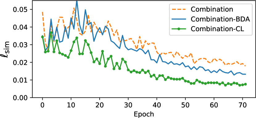
(a)

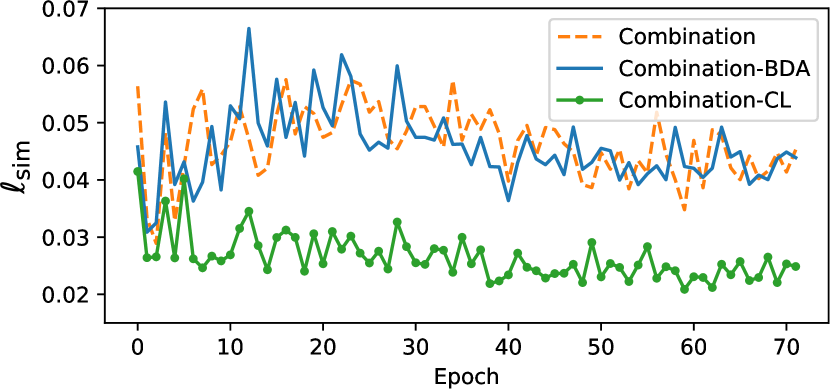
(b)

Fig. 1: The consistency loss, $\ell_{\mathsf{sim}}$, measured after each training epoch for the Combination models on (a) the training set and (b) the test set of the fold 1 split.

5 Conclusion

In this paper, we investigated consistency learning as a way to regularize the latent space of deep neural networks with respect to input transformations commonly used for data augmentation. We argued that enforcing consistency can benefit tasks such as audio classification. We proposed using the Jensen-Shannon divergence as a consistency loss term and used it to constrain the neural network output for several audio transformations. Experiments on the ESC-50 audio dataset demonstrated that our method can enhance existing data augmentation methods for audio classification and that consistency is enforced more effectively with an explicit loss term.

References

- [1] J. Salamon and J. P. Bello, “Deep convolutional neural networks and data augmentation for environmental sound classification,” IEEE Signal Processing Letters, vol. 24, no. 3, pp. 279–283, Jan. 2017.
- [2] D. S. Park, W. Chan, Y. Zhang, C. Chiu, B. Zoph, E. D. Cubuk, and Q. V. Le, “SpecAugment: A simple data augmentation method for automatic speech recognition,” in Proceedings of Interspeech, Graz, Austria, 2019, pp. 2613–2617.
- [3] U. Isik, R. Giri, N. Phansalkar, J-M. Valin, K. Helwani, and A. Krishnaswamy, “PoCoNet: Better speech enhancement with frequency-positional embeddings, semi-supervised conversational data, and biased loss,” in Proceedings of Interspeech, 2020, pp. 2487–2491.
- [4] Y. Bengio, A. Courville, and P. Vincent, “Representation learning: A review and new perspectives,” IEEE Transactions on Pattern Analysis and Machine Intelligence, vol. 35, no. 8, pp. 1798–1828, Aug. 2013.
- [5] S. Zheng, Y. Song, T. Leung, and I. Goodfellow, “Improving the robustness of deep neural networks via stability training,” in IEEE Conference on Computer Vision and Pattern Recognition (CVPR), Las Vegas, NV, USA, 2016, pp. 4480–4488.
- [6] D. Hendrycks, N. Mu, E. D. Cubuk, B. Zoph, J. Gilmer, and B. Lakshminarayanan, “AugMix: A simple data processing method to improve robustness and uncertainty,” in International Conference on Learning Representations (ICLR), 2020.
- [7] G. French, S. Laine, T. Aila, M. Mackiewicz, and G. Finlayson, “Semi-supervised semantic segmentation needs strong, varied perturbations,” in British Machine Vision Virtual Conference (BMVC), 2020.
- [8] F. Schroff, D. Kalenichenko, and J. Philbin, “FaceNet: A unified embedding for face recognition and clustering,” in IEEE Conference on Computer Vision and Pattern Recognition (CVPR), Boston, MA, USA, 2015, pp. 815–823.
- [9] T. Chen, S. Kornblith, M. Norouzi, and G. Hinton, “A simple framework for contrastive learning of visual representations,” in International Conference on Machine Learning (ICML), 2020.
- [10] A. Jansen, M. Plakal, R. Pandya, D. P. W. Ellis, S. Hershey, J. Liu, R. C. Moore, and R. A. Saurous, “Unsupervised learning of semantic audio representations,” in IEEE International Conference on Acoustics, Speech and Signal Processing (ICASSP), Calgary, AB, Canada, 2018, pp. 126–130.
- [11] N. Turpault, R. Serizel, and E. Vincent, “Semi-supervised triplet loss based learning of ambient audio embeddings,” in IEEE International Conference on Acoustics, Speech and Signal Processing (ICASSP), Brighton, UK, 2019, pp. 760–764.
- [12] K. J. Piczak, “ESC: Dataset for environmental sound classification,” in Proceedings of the 23rd ACM International Conference on Multimedia, New York, NY, USA, 2015, pp. 1015–1018.
- [13] Q. Xie, Z. Dai, E. Hovy, M. Luong, and Q. V. Le, “Unsupervised data augmentation for consistency training,” in Advances in Neural Information Processing Systems (NeurIPS), 2020.
- [14] S. Schneider, A. Baevski, R. Collobert, and M. Auli, “wav2vec: Unsupervised pre-training for speech recognition,” in Proceedings of Interspeech, Graz, Austria, 2019, pp. 3465–3469.
- [15] T. Miyato, S. Maeda, M. Koyama, and S. Ishii, “Virtual adversarial training: A regularization method for supervised and semi-supervised learning,” IEEE Transactions on Pattern Analysis and Machine Intelligence, vol. 41, no. 8, pp. 1979–1993, Jul. 2019.
- [16] F. L. Kreyssig and P. C. Woodland, “Cosine-distance virtual adversarial training for semi-supervised speaker-discriminative acoustic embeddings,” in Proceedings of Interspeech, 2020.
- [17] K. Simonyan and A. Zisserman, “Very deep convolutional networks for large-scale image recognition,” in International Conference on Learning Representations (ICLR), San Diego, CA, USA, 2015.
- [18] S. Ioffe and C. Szegedy, “Batch normalization: Accelerating deep network training by reducing internal covariate shift,” in International Conference on Machine Learning (ICML), Lille, France, 2015, vol. 37, pp. 448–456.
- [19] I. Loshchilov and F. Hutter, “Decoupled weight decay regularization,” in International Conference on Learning Representations (ICLR), New Orleans, LA, USA, 2019.
- [20] Q. Kong, Y. Cao, T. Iqbal, Y. Wang, W. Wang, and M. D. Plumbley, “PANNs: Large-scale pretrained audio neural networks for audio pattern recognition,” IEEE/ACM Transactions on Audio, Speech, and Language Processing, vol. 28, pp. 2880–2894, Oct. 2020.