CDPAM: Contrastive learning for perceptual audio similarity

Abstract

Many speech processing methods based on deep learning require an automatic and differentiable audio metric for the loss function. The Dpam approach of Manocha et al. [1] learns a full-reference metric trained directly on human judgments, and thus correlates well with human perception. However, it requires a large number of human annotations and does not generalize well outside the range of perturbations on which it was trained. This paper introduces Cdpam – a metric that builds on and advances Dpam. The primary improvement is to combine contrastive learning and multi-dimensional representations to build robust models from limited data. In addition, we collect human judgments on triplet comparisons to improve generalization to a broader range of audio perturbations. Cdpam correlates well with human responses across nine varied datasets. We also show that adding this metric to existing speech synthesis and enhancement methods yields significant improvement, as measured by objective and subjective tests.

Index Terms—  perceptual similarity, audio quality, deep metric, speech enhancement, speech synthesis

1 Introduction

Humans can easily compare and recognize differences between audio recordings, but automatic methods tend to focus on particular qualities and fail to generalize across the range of audio perception. Nevertheless, objective metrics are necessary for many automatic processing tasks that cannot incorporate a human in the loop. Traditional objective metrics like Pesq [2] and Visqol [3] are automatic and interpretable, as they rely on complex handcrafted rule-based systems. Unfortunately, they can be unstable even for small perturbations – and hence correlate poorly with human judgments.

Recent research has focused on learning speech quality from data [1, 4, 5, 6, 7, 8]. One approach trains the learner on subjective quality ratings, e.g., MOS scores on an absolute (1 to 5) scale [4, 5]. Such “no-reference” metrics support many applications but do not apply in cases that require comparison to ground truth, for example for learned speech synthesis or enhancement [9, 10].

Manocha et al. [1] propose a “full-reference” deep perceptual audio similarity metric (Dpam) trained on human judgments. As their dataset focuses on just-noticeable differences (JND), the learned model correlates well with human perception, even for small perturbations. However, the Dpam model suffers from a natural tension between the cost of data acquisition and generalization beyond that data. It requires a large set of human judgments to span the space of perturbations in which it can robustly compare audio clips. Moreover, inasmuch as its dataset is limited, the metric may generalize poorly to unseen speakers or content. Finally, because the data is focused near JNDs, it is likely to be less robust to large audio differences.

To ameliorate these limitations, this paper introduces Cdpam: a contrastive learning-based multi-dimensional deep perceptual audio similarity metric. The proposed metric builds on Dpam using three key ideas: (1) contrastive learning, (2) multi-dimensional representation learning, and (3) triplet learning. Contrastive learning is a form of self-supervised learning that augments a limited set of human annotations with synthetic (hence unlimited) data: perturbations to the data that should be perceived as different (or not). We use multi-dimensional representation learning to separately model content similarity (e.g. among speakers or utterances) and acoustic similarity (e.g. among recording environments). The combination of contrastive learning and multi-dimensional representation learning allows Cdpam to better generalize across content differences (e.g. unseen speakers) with limited human annotation [11, 12]. Finally, to further improve robustness to large perturbations (well beyond JND), we collect a dataset of judgments based on triplet comparisons, asking subjects: “Is A or B closer to reference C?”

We show that Cdpam correlates better than Dpam with MOS and triplet comparison tests across nine publicly available datasets. We observe that Cdpam is better able to capture differences due to subtle artifacts recognizable to humans but not by traditional metrics. Finally, we show that adding Cdpam to the loss function yields improvements to the existing state of the art models for speech synthesis [9] and enhancement [10]. The dataset, code, and resulting metric, as well as listening examples, are available here:
https://pixl.cs.princeton.edu/pubs/Manocha_2021_CCL/

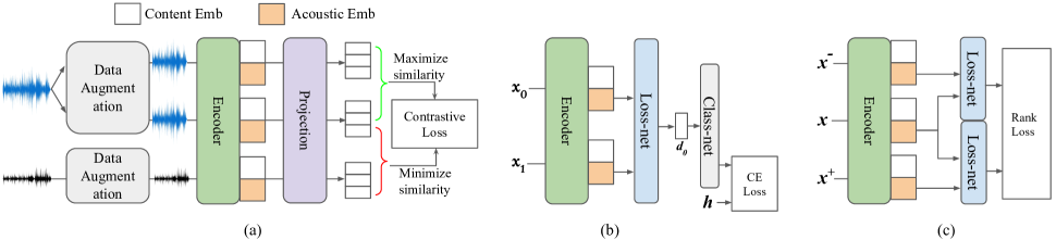
Fig. 1: Training architecture: (a) We first train an audio encoder using contrastive learning, then (b) train the loss-net on JND data [1]. (c) Finally, we fine-tune the loss-net on the newly collected dataset of triplet comparisons.

2 Related Work

2.1 Perceptual audio quality metrics

Pesq [2] and Visqol [3] were some of the earliest models to approximate the human perception of audio quality. Although useful, these had certain drawbacks: (i) sensitivity to perceptually invariant transformations [13]; (ii) narrow focus (e.g. telephony); and (iii) non-differentiable, making it impossible to be optimized for as an objective in deep learning. To overcome the last concern, researchers train differentiable models to approximate Pesq [7, 14]. The approach of Fu et al. [7] uses GANs to model Pesq, whereas the approach of Zhang et al. [14] uses gradient approximations of Pesq for training. Unfortunately, these approaches are not always optimizable, and may also fail to generalize to unseen perturbations.

Instead of using conventional metrics (e.g. Pesq) as a proxy, Manocha et al. [1] proposed Dpam that was trained directly on a new dataset of human JND judgments. Dpam correlates well with human judgment for small perturbations, but requires a large set of annotated judgments to generalize well across unseen perturbations. Recently, Serra et al. [8] proposed Sesqa trained using the same JND dataset [1], along with other datasets and objectives like Pesq. Our work is concurrent with theirs, but direct comparison is not yet available.

2.2 Representation learning

The ability to represent high-dimensional audio using compact representations has proven useful for many speech applications (e.g. speech recognition [15], audio retrieval [16]).

Multi-dimensional learning: Learning representations to identify the underlying explanatory factors make it easier to extract useful information on downstream tasks [17]. Recently in audio, Lee et al. [18] adapted Conditional Similarity Networks (CSN) for music similarity. The objective was to disentangle music into genre, mood, instrument, and tempo. Similarly, Hung et al. [19] explored disentangled representations for timbre and pitch of musical sounds useful for music editing. Chou et al. [20] explored the disentanglement of speaker characteristics from linguistic content in speech signals for voice conversion. Chen et al. [21] explored the idea of disentangling phonetic and speaker information for the task of audio representation.

Contrastive learning: Most of the work in audio has focused on audio representation learning [22, 23], speech recognition [24], and phoneme segmentation [25]. To the best of our knowledge, no prior method has used contrastive learning together with multi-dimensional representation learning to learn audio similarity.

3 The CDPAM Metric

This section describes how we train the metric in three stages, depicted in Fig 1: (a) pre-train the audio encoder using contrastive learning; (b) train the loss-net on the perceptual JND data; and (c) fine-tune the loss-net on the new perceptual triplet data.

3.1 Dataset

Self-supervised dataset: We borrow ideas from the SimCLR framework [26] for contrastive learning. SimCLR learns representations by maximizing agreement between differently augmented views of the same data example via a contrastive loss in the latent space. An audio is taken and transformations are applied to it to get a pair of augmented audio waveforms $x_{i}$ and $x_{j}$. Each waveform in that pair is passed through an encoder to get representations. These representations are further passed through a projection network to get final representations $z$. The task is to maximize the similarity between these two representations $z_{i}$ and $z_{j}$ for the same audio, in contrast to the representation $z_{k}$ on an unrelated piece of audio $x_{k}$.

In order to combine multi-dimensional representation learning with contrastive learning, we force our audio encoder to output two sets of embeddings: acoustic and content. We learn these separately using contrastive learning. To learn acoustic embedding, we consider data augmentation that takes the same acoustic perturbation parameters but different audio content, whereas to learn content embedding, we take different acoustic perturbation parameters but the same audio content. The pre-training dataset consists of roughly 100K examples.

JND dataset: We use the same dataset of crowd-sourced human perceptual judgments proposed by Manocha et al. [1]. In short, the dataset consists of around 55K pairs of human subjective judgments, each pair coming from the same utterance, with annotations of whether the two recordings are exactly the same or different? Perturbations consist of additive linear background noise, reverberation, coding/compression, equalization, and various miscellaneous noises like pops and dropouts.

Fine-tuning dataset: To make the metric robust to large (beyond JND) perturbations, we create a triplet comparison dataset. This improves the generalization performance of the metric to include a broader range of perturbations and also enhances the ordering of the learned space. We follow the same framework and perturbations as Manocha et al. [1]. This dataset consists of around 30K paired examples of crowd-sourced human judgments.

Type	Name	VoCo [27]	FFTnet [28]	BWE [29]	Dereverb	HiFi-GAN	PEASS	VC	Noizeus
Conventional	MSE	0.18	0.18	0.00	0.14	0.00	0.25	0.00	0.20
	Pesq	0.43	0.49	0.21	0.85	0.70	0.71	0.56	0.68
	VISQOL	0.50	0.02	0.13	0.75	0.69	0.66	0.49	0.61
1-10 JND metric	Dpam	0.71	0.63	0.61	0.45	0.30	0.63	0.45	0.10
1-10 Ours (default)	Cdpam	0.73	0.68	0.65	0.93	0.68	0.74	0.61	0.71

Table 1: Spearman correlation of models with various MOS tests. Models include conventional metrics, DPAM and ours. Higher is better.

3.2 Training and Architecture

Encoder Fig. 1(a): The audio encoder consists of a 16 layer CNN with $15\times 1$ kernels that is downsampled by half every fourth layer. We use global average pooling at the output to get a 1024-dimensional embedding, equally split into acoustic and content components. The projection network is a small fully-connected network that takes in a feature embedding of size 512 and outputs an embedding of 256 dimensions. The contrastive loss is taken over this projection. We use Adam [30] with a batch size of 16, learning rate of $10^{-4}$, and train for 250 epochs.

We use the NT-Xent loss (Normalized Temperature-Scaled Cross-Entropy Loss) proposed by Chen et al. [26]. The key is to map the two augmented versions of an audio (positive pair) with high similarity and all other examples in the batch (negative pairs) with low similarity. For measuring similarity, we use cosine distance. For more information, refer to SimCLR [26].

Loss-network Fig. 1(b-c): Our loss-net is a small 4 layer fully connected network that takes in the output of the audio encoder (acoustic embedding) and outputs a distance (using the aggregated sum of the L1 distance of deep features). This network also has a small classification network at the end that maps this distance to a predicted human judgment. Our loss-net is trained using binary cross-entropy between the predicted value and ground truth human judgment. We use Adam with a learning rate of $10^{-4}$, and train for 250 epochs. For fine-tuning on triplet data, we use MarginRankingLoss with a margin of $0.1$, using Adam with a learning rate of $10^{-4}$ for 100 epochs.

As part of online data augmentation to make the model invariant to small delay, we decide randomly if we want to add a 0.25s silence to the audio at the beginning or the end and then present it to the network. This helps to provide shift-invariance property to the model, to disambiguate that in fact the audio is similar when time-shifted. To also encourage amplitude invariance, we also randomly apply a small gain (-20dB to 0dB) on the training data.

Type	Name	FFTnet	BWE	HiFiGAN	Simulated
Conventional	MSE	55.0	49.0	70.2	43.0
	Pesq	67.1	38.1	88.5	86.1
	Visqol	64.2	44.4	96.1	84.2
1-6 JND metric	Dpam	61.5	87.7	93.2	71.8
1-6 Ours (default)	Cdpam	88.5	75.9	96.5	87.7

Table 2: 2AFC accuracy of various models, including conventional metrics, DPAM and ours. Higher is better.

4 Experiments

4.1 Subjective Validation

We use previously published diverse third-party studies to verify that our trained metric correlates well with their task. We show the results of our model and compare it with Dpam as well as more conventional objective metrics such as MSE, Pesq [2], and Visqol [3].

We compute the correlation between the model’s predicted distance with the publicly available MOS, using Spearman’s Rank order correlation (SC). These correlation scores are evaluated per speaker where we average scores for each speaker for each condition.

As an extension, we also check for 2AFC accuracy where we present one reference recording and two test recordings and ask subjects which one sounds more similar to the reference? Each triplet is evaluated by roughly 10 listeners. 2AFC checks for the exact ordering of similarity at per sample basis, whereas MOS checks for aggregated ordering, scale, and consistency. In addition to all evaluation datasets considered by Manocha et al. [1], we consider additional datasets:

1. Dereverberation [31]: consists of MOS tests to assess the performance of 5 deep learning-based speech enhancement methods.

2. HiFi-GAN [32]: consists of MOS and 2AFC scores to assess improvement across 10 deep learning based speech enhancement models (denoising and dereverberation).

3. PEASS [33]: consists of MOS scores to assess audio source separation performance across 4 metrics: global quality, preservation of target source, suppression of other sources, and absence of additional artifacts. Here, we only look at global quality.

4. Voice Conversion (VC) [34]: consists of tasks to judge the performance of various voice conversion systems trained using parallel (HUB) and non-parallel data (SPO). Here we only consider HUB.

5. Noizeus [35]: consists of a large scale MOS study of non-deep learning-based speech enhancement systems across 3 metrics: SIG-speech signal alone; BAK-background noise; and OVRL-overall quality. Here, we only look at OVRL.

Results are displayed in Tables 1 and 2, in which our proposed metric has the best performance overall. Next, we summarize with a few observations:

• Similar to findings by Manocha et al. [1], conventional metrics like Pesq and Visqol perform better on measuring large distances (e.g. Dereverb, HiFi-GAN) than subtle differences (e.g. BWE), suggesting that these metrics do not correlate well with human perception when measuring subtle differences.

• We observe a natural compromise between generalizing to large audio differences well beyond JND (e.g. FFTnet, VoCo, etc.) and focusing only on small differences (e.g. BWE). As we see, Cdpam is able to correlate well across a wide variety of datasets, whereas Dpam correlates best where the audio differences are near JND. Cdpam scores higher than Dpam on BWE on MOS correlation, but has a lower 2AFC score suggesting that Dpam might be better at ordering individual pairwise judgments closer to JND.

• Compared to Dpam, Cdpam performs better across a wide variety of tasks and perturbations, showing higher generalizability across perturbations and downstream tasks.

Name	ComArea$\downarrow$	Mono$\uparrow$	VoCo$\uparrow$	FFTnet$\uparrow$	BWE$\uparrow$
Dpam [1]	0.76	0.89	-	-	-
1-6 self-sup. (triplet m.learning)	0.52	0.31	0.21	0.10	0.00
contrastive w/o mul-dim. rep.	0.43	0.48	0.38	0.17	0.38
self-sup. (contrastive)	0.34	0.53	0.34	0.58	0.60
+JND	0.32	0.88	0.65	0.65	0.79
+JND+fine-tune (default)	0.32	0.89	0.73	0.68	0.65

Table 3: Ablation studies. Sec 4.2 describes common area, monotonicity, and Spearman correlations for 3 datasets. $\uparrow$ or $\downarrow$ is better.

4.2 Ablation study

We perform ablation studies to better understand the influence of different components of our metric in Table 3. We compare our trained metric at various stages: (i) after self-supervised training; (ii) after JND training; and (iii) after triplet finetuning (default). To further compare amongst self-supervised approaches, we also show results of self-supervised metric learning using triplet loss. To also show improvements due to learning multi-dimensional representations, we show results of a model trained using contrastive learning without content dimension. The metrics are compared on (i) robustness to content variations; (ii) monotonic behavior with increasing perturbation levels; and (iii) correlation with subjective ratings from a subset of existing datasets.

Robust to content variations To evaluate robustness to content variations, we create a test dataset of two groups: one consisting of pairs of recordings that have the same acoustic perturbation levels but varying audio content; the other consisting of pairs of recordings having different perturbation levels and audio content. We calculate the common area between these normalized distributions. Our final metric has the lowest common area, suggesting that it is more robust to changing audio content. Decreasing common area also corresponds with increasing MOS correlations across downstream tasks, suggesting that the task of separating these two distribution groups may be a factor when learning acoustic audio similarity.

Clustered Acoustic Space: To further quantify this learned space, we also calculate the Precision of Top $K$ retrievals which measures the quality of top $K$ items in the ranked list. Given 10 different acoustic perturbation groups - each group consisting of 100 files having the same acoustic perturbation levels but different audio content, we take randomly selected queries and calculate the number of correct class instances in the top $K$ retrievals. We report the mean of this metric over all queries ($MP^{k}$). Cdpam gets $MP^{k=10}$ = 0.92 and $MP^{k=20}$ = 0.87, suggesting that these acoustic perturbation groups all cluster together in the learned space.

Monotonicity To show our metric’s monotonicity with increasing levels of noise, we create a test dataset of recordings with different audio content and increasing noise perturbation levels (both individual and combined perturbations). We calculate SC between the distance from the metric and the perturbation levels. Both Dpam and Cdpam behave equally monotonically with increasing levels of noise.

MOS Correlations Each of the key components of Cdpam  namely contrastive-learning, multi-dimensional representation learning, and triplet learning have a significant impact on generalization across downstream tasks. Surprisingly, even our self-supervised model has a non-trivial positive correlation with increasing noise as well as MOS correlation across datasets. This suggests that a self-supervised model not trained on any classification or perceptual task is still able to learn useful perceptual knowledge. This is true across datasets ranging from subtle to large differences suggesting that contrastive learning can be a useful pre-training strategy.

4.3 Waveform generation using our learned loss

We show the utility of our trained metric as a loss function for the task of waveform generation. We use the current state-of-the-art MelGAN [9] vocoder. We train two models: i) single speaker model trained on LJ [36], and ii) cross-speaker model trained on a subset of VCTK [37]. Both the models were trained for around 2 million iterations until convergence. We take the existing model and just add Cdpam as an additional loss in the training objective.

We randomly select 500 unseen audio recordings to evaluate results. For the single-speaker model, we use LJ dataset, whereas for the cross-speaker model, we use the 20 speaker DAPS [38] dataset. We perform A/B preference tests on Amazon Mechanical Turk (AMT), consisting of Ours vs baseline pairwise comparisons. Each pair is rated by 6 different subjects and then majority voted to see which method performs better per utterance. As shown in Fig 2(a), our models outperform the baseline in both categories. All results are statistically significant with p $<$ $10^{-4}$. Our model is strongly preferred over the baseline, but the maximum improvement is observed in the cross-speaker scenario where our model performs best. Specifically, we observe that MelGAN enhanced with Cdpam detects and follows the reference pitch better than the baseline.

	Pesq	STOI	CSIG	CBAK	COVL	MOS
Noisy	1.97	91.50	3.35	2.44	2.63	2.61
DEMUCS [10]	3.01	95.00	4.39	3.44	3.73	3.73
DEMUCS+Cdpam	3.10	95.07	4.46	3.55	3.82	3.86
Finetune Cdpam	3.06	94.93	4.30	3.56	3.70	4.07

Table 4: Evaluation of denoising models using the VCTK [37] test set with four objective measures and one subjective measure.

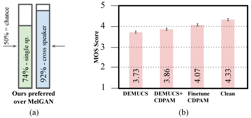
Fig. 2: Subjective tests: (a) In pairwise tests, ours is typically preferred over MelGAN for single speaker and cross-speaker synthesis. (b) MOS tests show denoising methods are improved by CDPAM.

4.4 Speech Enhancement using our learned loss

To further demonstrate the effectiveness of our metric, we use the current state-of-the-art DEMUCS architecture based speech denoiser [10] and supplement Cdpam in two ways: (i) DEMUCS+CDPAM: train from scratch using a combination of L1, multi-resolution STFT and Cdpam; and (ii) Fintune Cdpam: pre-train on L1 and multi-resolution STFT loss and finetune on Cdpam. The training dataset consists of VCTK [37] and DNS [39] datasets. For a fair comparison, we only compare real-time (causal) models.

We randomly select 500 audio clips from the VCTK test set and evaluate scores on that dataset. We evaluate the quality of enhanced speech using both objective and subjective measures. For the objective measures, we use: i) Pesq (from 0.5 to 4.5); (ii) Short-Time Objective Intelligibility (STOI) (from 0 to 100); (iii) CSIG: MOS prediction of the signal distortion attending only to the speech signal (from 1 to 5); (iv) CBAK: MOS prediction of the intrusiveness of background noise (from 1 to 5); (v) COVL: MOS prediction of the overall effect (from 1 to 5). We compare the baseline model with both our models. Results are shown in Table 4.

For subjective studies, we conducted a MOS listening study on AMT where each subject is asked to rate the sound quality of an audio snippet on a scale of 1 to 5, with 1=Bad, 5=Excellent. In total, we collect around 1200 ratings for each method. We provide studio-quality audio as reference for high-quality, and the input noisy audio as low-anchor. As shown in Fig 2(b), both our models perform better than the baseline approach. We observe that our Finetune Cdpam model scores the highest MOS score. This highlights the usefulness of using Cdpam in audio similarity tasks. Specifically, Cdpam can identify and eliminate minor human perceptible artifacts that are not captured by traditional losses. We also note that higher objective scores do not guarantee higher MOS, further motivating the need for better objective metrics.

5 Conclusion and Future work

In this paper, we present Cdpam, a contrastive learning-based deep perceptual audio metric that correlates well with human subjective ratings across tasks. The approach relies on multi-dimensional and self-supervised learning to augment limited human-labeled data. We show the utility of the learned metric as an optimization objective for speech synthesis and enhancement, but it could be applied in many other applications. We would like to extend this metric to include content similarity as well, in general going beyond acoustic similarity for applications like music similarity. Though we showed two applications of the metric, future works could also explore other applications like audio retrieval and speech recognition.

References

- [1] P. Manocha, A. Finkelstein, et al., “A differentiable perceptual audio metric learned from just noticeable differences,” in Interspeech, 2020.
- [2] A. W. Rix, J. G. Beerends, M. P. Hollier, and A. P. Hekstra, “Perceptual evaluation of speech quality (PESQ)-a new method for speech quality assessment,” in ICASSP, 2001.
- [3] A. Hines, J. Skoglund, A C. Kokaram, et al., “ViSQOL: an objective speech quality model,” EURASIP Journal on Audio, Speech, and Music Processing, 2015.
- [4] C-C. Lo, S-W. Fu, W-C. Huang, X. Wang, Junichi Yamagishi, Yu Tsao, and Hsin-Min Wang, “MOSNet: Deep learning based objective assessment for voice conversion,” Interspeech, 2019.
- [5] B. Patton, Y. Agiomyrgiannakis, M. Terry, K. Wilson, R. A. Saurous, and D. Sculley, “AutoMOS: Learning a non-intrusive assessor of naturalness-of-speech,” in NIPS Workshop, 2016.
- [6] S-W. Fu, C-F. Liao, and Y. Tsao, “Learning with learned loss function: Speech enhancement with quality-net,” SPS, vol. 27, pp. 26–30, 2019.
- [7] S-W. Fu, C-F. Liao, Y. Tsao, and S.D. Lin, “MetricGAN: Generative adversarial networks based black-box metric scores optimization for speech enhancement,” in ICML, 2019.
- [8] J. Serrà, J. Pons, et al., “SESQA: semi-supervised learning for speech quality assessment,” arXiv:2010.00368, 2020.
- [9] K. Kumar, R. Kumar, T. de Boissiere, L. Gestin, W. Z. Teoh, J. Sotelo, A. de Brebisson, Y. Bengio, and A. Courville, “Melgan: Generative adversarial networks for conditional waveform synthesis,” in NeurIPS, 2019.
- [10] A. Defossez, G. Synnaeve, and Y. Adi, “Real time speech enhancement in the waveform domain,” in Interspeech, 2020.
- [11] S V. Steenkiste, F. Locatello, J. Schmidhuber, and O. Bachem, “Are disentangled representations helpful for abstract visual reasoning?,” in NeurIPS, 2019.
- [12] I. Higgins, D. Amos, D. Pfau, S. Racaniere, L. Matthey, D. Rezende, and A. Lerchner, “Towards a definition of disentangled representations,” arXiv:1812.02230, 2018.
- [13] A. Hines, J. Skoglund, A. Kokaram, and N. Harte, “Robustness of speech quality metrics: Comparing ViSQOL, PESQ and POLQA,” in ICASSP, 2013.
- [14] H. Zhang, X. Zhang, and G. Gao, “Training supervised speech separation system to improve STOI and PESQ directly,” in ICASSP, 2018.
- [15] A. Conneau, A. Baevski, et al., “Unsupervised cross-lingual representation learning for speech recognition,” arXiv:2006.13979, 2020.
- [16] P. Manocha, R. Badlani, A. Kumar, A. Shah, B. Elizalde, and B. Raj, “Content-based representations of audio using siamese neural networks,” in ICASSP, 2018.
- [17] Y. Bengio, A. Courville, and P. Vincent, “Representation learning: A review and new perspectives,” PAML, 2013.
- [18] J. Lee, N J. Bryan, J. Salamon, Z. Jin, and J. Nam, “Disentangled multidimensional metric learning for music similarity,” in ICASSP, 2020.
- [19] Y N. Hung, Y A. Chen, and Y H. Yang, “Learning disentangled representations for timber and pitch in music audio,” in arXiv:1811.03271, 2018.
- [20] J. Chou, C. Yeh, H. Lee, and L. Lee, “Multi-target voice conversion without parallel data by adversarially learning disentangled audio representations,” in arXiv:1804.02812, 2018.
- [21] Y.C. Chen, S.F. Huang, H.Y. Lee, Y.H. Wang, and C.H. Shen, “Audio word2vec: Sequence-to-sequence autoencoding for unsupervised learning of audio segmentation and representation,” ASLP, 2019.
- [22] A. Oord, Y. Li, and O. Vinyals, “Representation learning with contrastive predictive coding,” in arXiv:1807.03748, 2018.
- [23] P. Chi, P. Chung, T. Wu, et al., “Audio Albert: A lite BERT for self-supervised learning of audio representation,” in arXiv:2005.08575, 2020.
- [24] S. Schneider, A. Baevski, R. Collobert, and M. Auli, “wav2vec: Unsupervised pre-training for speech recognition,” in Interspeech, 2019.
- [25] F. Kreuk, J. Keshet, and Y. Adi, “Self-supervised contrastive learning for unsupervised phoneme segmentation,” in Interspeech, 2020.
- [26] T. Chen, S. Kornblith, M. Norouzi, and G. Hinton, “A simple framework for contrastive learning of visual representations,” in ICML, 2020.
- [27] Z. Jin, G J. Mysore, S. Diverdi, J. Lu, and A. Finkelstein, “Voco: Text-based insertion and replacement in audio narration,” TOG, 2017.
- [28] Z. Jin, A. Finkelstein, G J. Mysore, and J. Lu, “FFTNet: A real-time speaker-dependent neural vocoder,” in ICASSP, 2018.
- [29] B. Feng, Z. Jin, J. Su, and A. Finkelstein, “Learning bandwidth expansion using perceptually-motivated loss,” in ICASSP, 2019.
- [30] D P. Kingma and J. Ba, “Adam: A method for stochastic optimization,” in ICLR, 2015.
- [31] J. Su, A. Finkelstein, and Z. Jin, “Perceptually-motivated environment-specific speech enhancement,” in ICASSP, 2019.
- [32] J. Su, Z. Jin, et al., “HiFi-GAN: High-fidelity denoising and dereverberation,” Interspeech, 2020.
- [33] V. Emiya, E. Vincent, N. Harlander, et al., “Subjective and objective quality assessment of audio source separation,” ASLR, 2011.
- [34] J. Lorenzo-Trueba, J. Yamagishi, T. Toda, D. Saito, F. Villavicencio, T. Kinnunen, and Z. Ling, “The voice conversion challenge 2018,” arXiv:1804.04262, 2018.
- [35] Y. Hu and P. C. Loizou, “Subjective comparison and evaluation of speech enhancement algorithms,” Speech communication, 2007.
- [36] K. Ito et al., “The LJ speech dataset,” 2017.
- [37] C. Valentini-Botinhao et al., “Noisy speech database for training speech enhancement algorithms and TTS models,” 2017.
- [38] G J. Mysore, “Can we automatically transform speech recorded on common consumer devices in real-world environments into professional production quality speech?—a dataset, insights, and challenges,” SPS, 2014.
- [39] C K. Reddy, E. Beyrami, H. Dubey, V. Gopal, et al., “The interspeech 2020 deep noise suppression challenge: Datasets, subjective speech quality and testing framework,” Interspeech, 2020.