Towards Bridging the gap between Empirical and Certified Robustness against Adversarial Examples

Abstract

The current state-of-the-art defense methods against adversarial examples typically focus on improving either empirical or certified robustness. Among them, adversarially trained (AT) models produce empirical state-of-the-art defense against adversarial examples without providing any robustness guarantees for large classifiers or higher-dimensional inputs. In contrast, existing randomized smoothing based models achieve state-of-the-art certified robustness while significantly degrading the empirical robustness against adversarial examples. In this paper, we propose a novel method, called Certification through Adaptation, that transforms an AT model into a randomized smoothing classifier during inference to provide certified robustness for $\ell_{2}$ norm without affecting their empirical robustness against adversarial attacks. We also propose Auto-Noise technique that efficiently approximates the appropriate noise levels to flexibly certify the test examples using randomized smoothing technique. Our proposed Certification through Adaptation with Auto-Noise technique achieves an average certified radius (ACR) scores up to $1.102$ and $1.148$ respectively for CIFAR-10 and ImageNet datasets using AT models without affecting their empirical robustness or benign accuracy. Therefore, our paper is a step towards bridging the gap between the empirical and certified robustness against adversarial examples by achieving both using the same classifier.

1 Introduction

Deep neural network (DNN) based models are found to be brittle to minor, adversarially-chosen perturbations for their inputs that remain undetectable to human eyes. A DNN classifier that correctly classifies a clean image $x$, can be easily fooled by choosing such adversarial attacks to misclassify $x+\delta$ (Szegedy et al., 2014; Goodfellow et al., 2015; Madry et al., 2018). Here, $\delta$ is a minor adversarial perturbation such that the change between $x$ and $x+\delta$ remains imperceptible.

Among the existing successful defense models, adversarial training (AT) produces the best empirical robustness against the known adversarial attacks, however, without providing any guarantee Madry et al. (2018); Tramèr & Boneh (2019); Zhang et al. (2019); Rice et al. (2020); Gowal et al. (2020). It trains a DNN classifier using strong adversaries from a specific class of perturbation (e.g., a small $\ell_{p}$-norm) to provide robustness for the same perturbation types. Several certification techniques are proposed that can be applied to adversarially trained models to certifiably verify if the prediction of a test example, $x$ remains constant within its neighborhood Wong & Kolter (2018); Wang et al. (2018); Salman et al. (2019b); Dvijotham et al. (2018); Gehr et al. (2018); Sheikholeslami et al. (2021). However, these certification techniques typically do not scale for larger networks (e.g., ResNet50) and datasets (e.g., ImageNet). Hence, we cannot guarantee for large networks or data-sets that a powerful, not yet known attack would not break these defenses. In fact, several recently proposed empirical defense models are later broken by stronger adaptive adversarial attacks, indicating the importance of investigating certified defenses with suitable robustness guarantees Carlini & Wagner (2017); Athalye et al. (2018). In contrast to these models, the randomized smoothing based models can provide scalable $\ell_{2}$-certification framework for any classification model, which is robust against large isotropic Gaussian noise (Cohen et al., 2019; Salman et al., 2019a). However, the existing randomized smoothing-based models significantly degrade the empirical robustness compared to the state-of-the-art AT models. In summary, a high empirical robustness along with certification guarantees are necessary to improve the reliability of a DNN model for sensitive real-world applications. However, to the best of our knowledge, none of the existing techniques provide both high performance for both empirical robustness with such certified guarantees using the same DNN classifier. Towards this, we aim to bridge this gap by providing robustness certification for AT models without degrading their state-of-the-art empirical robustness against adversarial examples.

CIFAR-10 models with the best hyper-parameters for $\ell_{2}$ certifications
$\ell_{2}$ Radius	0.0	0.25	0.5	0.75	1.0	1.25	1.5	1.75	2.0	2.25	2.5	2.75	3.0	ACR
Baseline	10.49	6.96	2.04	0.09	0.0	0.0	0.0	0.0	0.0	0.0	0.0	0.0	0.0	0.035
Baseline + Auto-Noise	33.57	18.56	10.25	4.44	0.83	0.07	0.01	0.0	0.0	0.0	0.0	0.0	0.0	0.124
Baseline + Adaptation + Auto-Noise	59.64	21.66	7.81	3.97	1.28	0.36	0.07	0.0	0.0	0.0	0.0	0.0	0.0	0.154
Randσ=0.5 (Cohen et al., 2019)	62.13	51.68	40.38	30.25	20.81	13.36	7.71	3.38	0.0	0.0	0.0	0.0	0.0	0.494
Randσ=0.5 + Auto-Noise	79.48	71.75	60.23	48.72	35.97	25.16	15.09	10.13	6.98	5.58	4.18	2.94	1.76	0.821
Randσ=0.5 + Adaptation + Auto-Noise	78.27	69.51	57.16	44.73	31.19	19.27	10.4	4.25	1.65	0.57	0.14	0.01	0.0	0.695
SmoothAdvσ=0.5 (Salman et al., 2019a)	57.59	52.82	47.67	42.68	37.55	32.64	27.52	22.42	0.0	0.0	0.0	0.0	0.0	0.733
SmoothAdvσ=0.5 + Auto-Noise	61.27	57.27	52.52	48.17	43.49	38.02	33.15	27.47	21.86	15.81	9.5	4.97	2.01	0.965
SmoothAdvσ=0.5 + Adaptation + Auto-Noise	61.23	56.9	51.33	46.44	41.05	35.65	30.11	24.35	18.48	12.8	7.76	4.27	2.3	0.908
Adv∞ (Rice et al., 2020)	13.82	12.22	10.48	9.12	7.69	6.32	5.1	3.79	0.0	0.0	0.0	0.0	0.0	0.154
Adv∞ + Auto-Noise	69.46	63.12	35.73	30.63	17.54	14.78	10.27	9.16	8.01	7.2	6.21	5.31	3.78	0.649
Adv∞ + Adaptation + Auto-Noise	70.75	64.54	50.63	43.38	32.5	24.43	18.05	12.2	8.31	5.37	3.36	1.96	1.23	0.76
Adv2 (Rice et al., 2020)	30.37	26.98	23.98	21.35	18.4	15.94	13.52	10.63	0.0	0.0	0.0	0.0	0.0	0.367
Adv2 + Auto-Noise	64.45	60.57	45.73	41.06	28.48	22.92	15.1	10.77	7.23	4.8	2.77	1.67	1.1	0.702
Adv2 + Adaptation + Auto-Noise	61.96	58.58	53.64	49.67	42.76	38.69	34.54	30.36	24.65	20.77	17.09	13.66	9.18	1.102
Marcerσ=0.5 (Zhai et al., 2020)	64.2	57.5	49.9	42.3	34.8	27.6	20.2	12.6	0.0	0.0	0.0	0.0	0.0	0.691
Consistencyσ=0.5 (Jeong & Shin, 2020)	52.3	48.9	45.1	41.3	37.8	33.9	29.9	25.2	0.0	0.0	0.0	0.0	0.0	0.726
Boostingσ=0.5 (Horváth et al., 2022)	65.0	59.0	49.4	44.8	38.6	32.0	26.2	19.8	0.0	0.0	0.0	0.0	0.0	0.756

Table 1: CIFAR-10: Certified accuracy at different $\ell_{2}$ radii and ACR scores using the best hyper-parameters. Existing randomized-smoothing based models are trained and certified using noise-level, $\sigma=0.5$. We also present the best reported results for Marcer and Consistency at (Jeong & Shin, 2020) and for Boosting at (Horváth et al., 2022) for our comparisons. For detailed results and hyper-parameters for both ImageNet and CIFAR-10 datasets, please refer to Table 3 and 4 respectively in Appendix.

In this paper, we propose a novel certification through adaptation framework that transforms an AT model into a randomized smoothing framework during inference to provide non-trivial $\ell_{2}$ certification without any additional training or architecture modifications. Our proposed certification technique consists of two steps: We first adapt the AT model using popular batch normalization adaptation technique using appropriate levels of Gaussian noises separately for each test example (Cariucci et al., 2017; Li et al., 2016). This process significantly boosts the performance of the AT models against the random isotropic Gaussian noises. Hence, we can now directly apply the randomized smoothing based certification technique to provide $\ell_{2}$ certification in the next step. However, choosing the Gaussian noise for each test example is a challenging task. The existing randomized smoothing based models that use Gaussian noises for training, use the same noise levels to certify each test example, significantly compromising their certification performance. Towards this, we also propose an Auto-Noise technique to efficiently approximate the appropriate Gaussian noise levels for correctly certifying each test example during inference.

In the following, we summarize the list of contributions for our paper:

1. We propose a novel certification through adaptation framework that adapts an AT model using Gaussian noises to provide non-trivial robustness certifications at large $\ell_{2}$ radii. Our proposed technique only requires a set of clean images, obtained from training/validation or test set to adapt the AT models using popular BN-adaptation technique (Cariucci et al., 2017; Li et al., 2016).

2. We also propose Auto-Noise technique to efficiently approximate the appropriate Gaussian noise levels for certifying each test example during inference. Auto-Noise is applicable even for existing randomized smoothing based models and often significantly improves the certification performance. Our Certification through Adaptation together with Auto-Noise technique produces average certified radius (ACR) scores upto $1.102$ and $1.148$ for CIFAR-10 and ImageNet for AT models, achieving the state-of-the-art performance for CIFAR-10. Notably, our proposed method is applied during inference, without affecting the empirical robustness or benign accuracy of AT models to produce these non-trivial $\ell_{2}$ certification results.

3. Our results also suggests a stronger correlation between empirical and certified robustness that empirically stronger AT models also produce better $\ell_{2}$ certification performance.

2 Related Work

2.1 Adversarial Robustness for DNN models

Empirical Defenses and Adversarial Training. Defense models against adversarial examples can be broadly categorized as: empirical and certified defenses. Empirical defenses demonstrate empirical robustness against adversarial attacks, typically without out providing any certification guarantees (Schott et al., 2019; Moosavi Dezfooli et al., 2019; Nandy et al., 2020; Mao et al., 2021). Adversarial training achieves the state-of-the-art empirical defense (Madry et al., 2018). It optimizes the following loss function for a DNN classifier, $f$, to provide robustness within an $\epsilon$-bounded threat model for an $\ell_{p}$ norm, where the perturbations, $\delta\in\Delta$ are constrained as $\Delta=\{\delta:||\delta||_{p}\leq\epsilon\}$:

$$\min_{\theta}\mathbb{E}_{(x,y)}[\max_{\delta\in\Delta}\mathcal{L}(f_{\theta}(x+\delta),y)]$$ (1)

where, $\theta$ denotes the model parameters. $\mathcal{L}$ is the classification loss.

The inner maximization in Eq. 1 is solved by producing adversarial examples using strong iterative adversaries, e.g., projected gradient descent (PGD) attack (Kurakin et al., 2016; Madry et al., 2018). Wong et al. (2020) found that even a single-step fast gradient sign method (FGSM) attack-based AT models also achieves high empirical robustness (Goodfellow et al., 2015). Zhang et al. (2020) proposed to use the least adversaries for training. Recently TRADES (Zhang et al., 2019), Adv-LLR (Qin et al., 2019) introduced additional regularizers to achieve higher empirical robustness by smoothing the loss surface. Rice et al. (2020) showed that even the standard PGD based AT model with early-stopping criteria provides one of the best empirical defenses for a given perturbation type. Recent works also explored the importance of different hyper-parameters for adversarial training (Gowal et al., 2020; Pang et al., 2021) as well as incorporating additional data in a semi-supervised fashion (Carmon et al., 2019; Uesato et al., 2019) to further improve their empirical robustness against adversarial attacks. Recently, Kireev et al. (2021) also demonstrated that adversarial training with smaller perturbation can also improve the performance against random corruptions.

Certified Defenses. Empirical defenses demonstrate robustness only against the known adversaries without providing any guarantees. In fact, most empirical defenses proposed in the literature were later broken by stronger adversaries, highlighting the importance of certified defenses to provide robustness guarantees (Athalye et al., 2018; Uesato et al., 2018; Jalal et al., 2019).

Several recent works proposed to train neural network models with provable robustness guarantees. These works include methods based on semidefinite relaxations (Raghunathan et al., 2018), linear relaxations and duality (Wong & Kolter, 2018; Wong et al., 2018), abstract interpretation (Mirman et al., 2018), and interval bound propagation (Gowal et al., 2018). Parallel to training a certified defense, several works also focus on certifying the already trained models (Tjeng et al., 2017; Gehr et al., 2018; Weng et al., 2018; Wang et al., 2018; Bunel et al., 2018). Recently Mueller et al. (2021) combined a small certification network with a large, empirically robust AT model using some selection criteria to boost overall benign accuracy along with empirical robustness for the certified framework. However, most of these techniques do not scale well for large DNN classifiers (e.g., ResNet50) or higher-dimensional datasets (e.g., ImageNet).

Randomized Smoothing is a promising certification technique that can be scaled to larger networks and higher-dimensional datasets. It was initially proposed as a heuristic defense (Cao & Gong, 2017; Liu et al., 2018) and later shown to be certifiable (Lecuyer et al., 2019; Li et al., 2019). Recently, Cohen et al. (2019) and Salman et al. (2019a) separately provided strong robustness guarantees for $\ell_{2}$-norm. A randomized smoothing based certification model requires their base-classifier to be robust against large Gaussian perturbations to produce non-trivial results. Cohen et al. (2019) proposed to train their base-classifier by incorporating random Gaussian noises. Several recent works focused on improving the base classifiers to achieve better certification performance by adversarially choosing the noise (Salman et al., 2019a), incorporating additional regularizers (Zhai et al., 2020; Jeong & Shin, 2020), by ensembling multiple base-models (Horváth et al., 2022) etc. Several works also investigated on improving certification guarantees using different smoothing measures (Li et al., 2019; Lee et al., 2019; Yang et al., 2020) or divergences (Dvijotham et al., 2020). Salman et al. (2020); Carlini et al. (2022) demonstrated that we can achieve non-trivial certified robustness even for a standard DNN classifier by incorporating an additional denoising module as a pre-processing unit. Notably, randomized smoothing is the only scalable certification framework and also provides superior performance for different perturbation types (Dvijotham et al., 2020).

However, while achieving the state-of-the-art certification performance, randomized smoothing significantly degrades the empirical robustness against adversarial attacks compared to the state-of-the-art AT models (Lecuyer et al., 2019; Salman et al., 2019a; Cohen et al., 2019). Towards this, our proposed technique transforms an AT model into a randomized smoothing classifier without requiring additional training or architectural modification. Since AT models already provide the state-of-the-art empirical defense, we achieve both empirical and certified robustness against adversarial examples using the same classifier.

Batch-normalization and Robustness. Several recent papers investigate the effects of batch-normalization layers for different aspects of robustness. Many of these works focused on improving robustness against random corruptions by adapting batch-normalization using a sufficiently large set of test images from the same covariate shift (Schneider et al., 2020; Nado et al., 2020; Benz et al., 2021a). By hypothesizing that clean and adversarial examples belongs to different domains, several recent works proposed to apply different branches of BN to separately capture their distributions (Xie et al., 2020a; Xie & Yuille, 2020; Jiang et al., 2020; Wang et al., 2020b; 2021). Benz et al. (2021b) presents empirical evidence to argue that BN shifts a model towards being more dependent on non-robust features (NRFs). Unlike these previous works, we proposed to adapt BN layers using appropriate Gaussian noise levels to provide $\ell_{2}$ certified robustness for AT models.

2.2 Test-time Adaptation & applications

Test-time adaptation techniques have been widely explored before in the field of domain adaptation (Sun et al., 2017; Roy et al., 2019; Huang et al., 2018; Li et al., 2016) and covariate-shift adaptation (Sun et al., 2020; French et al., 2017; Xie et al., 2020b; Wang et al., 2020a; Schneider et al., 2020; Nado et al., 2020; Benz et al., 2021a). However, to the best of our knowledge, such techniques are never applied for adversarial robustness and certification. Our paper mainly focuses on one of the most popular and effective mechanisms, called adaptive batch-normalization.

A batch-normalization (BN) layer computes the mean and variance of the hidden activation maps across the channels to normalize these activations to $\mathcal{N}(0,1)$ before feeding into the next hidden layer (Ioffe & Szegedy, 2015). This process reduces the dependencies among different hidden layers, improving the training efficiency for deep architectures. However, the distributional shifts in the test examples lead to different activation statistics compared to the training examples. Hence, the statistics estimated during training fail to correctly normalize the activation tensors to $\mathcal{N}(0,1)$. Consequently, it breaks the crucial assumption for the subsequent hidden layers to work. Adaptive BN technique computes the BN statistics from the feature activations, $\mu_{t}$, $s_{t}^{2}$, of the test batch. We can adapt them with the existing training statistics, $\mu_{T}$, $s_{T}^{2}$, learned using the training batches as (Cariucci et al., 2017; Li et al., 2016; Schneider et al., 2020):

$$\overline{\mu}=\rho\cdot\mu_{t}+(1-\rho)\cdot\mu_{T}\quad\overline{s}=\rho\cdot s_{t}+(1-\rho)\cdot s_{T}$$ (2)

where, $\rho\in[0,1]$ is the momentum. The choice of $\rho=0$ is equivalent to the standard inference setup with a deterministic DNN classifier in the IID settings. We should choose $\rho=1$ when receiving larger test batches as it can provide a better estimation of the test distributions.

Assumptions and Limitations. The existing BN-adaptation techniques typically require a large set of test images from the same “unknown” test distributions. However, this assumption may not hold for several real-world applications, e.g., stateless web APIs. Also, these test images should be semantically diverse, preferably over multiple classes, to effectively estimate the test distributions. Hence, it further limits the practical usability of these frameworks for real-world applications, e.g., autonomous cars.

Unlike these models for domain adaptation and corruption robustness, our proposed certification framework does not make any such assumptions. As we shall see that we can appropriately approximate the required Gaussian noise level for adaptation to certify a test image. Therefore, we can pre-select a diverse set of clean images, $\mathbf{X}_{clean}$ and inject the random Gaussian noises to appropriately adapt the models as required, addressing both of these limitations.

3 Proposed Methodology

In this section, we first present the background of the randomized smoothing technique and explain why it is not directly applicable to AT models. Next, we present our proposed certification through adaptation framework that adapts a DNN model during inference to provide certified robustness without additional training or architectural modifications.

3.1 Background on Randomized Smoothing

Consider a classification model, $f$, that maps inputs in $\mathbb{R}^{d}$ to $\mathcal{Y}$ classes. The randomized smoothing framework transforms the original base classifier, $f$ into a new, smoothed classifier $g$ Cohen et al. (2019). In particular, for an input $x\in\mathbb{R}^{d}$, the smoothed classifier $g$ returns the most probable class to be predicted by the base classifier $f$ under isotropic Gaussian noises of $x$. That is,

$$g(x)=arg\max_{y\in\mathcal{Y}}\mathbb{P}(f(x+\delta)==y)\quad\text{s.t.}~{}~{}\delta\sim\mathcal{N}(0,\sigma^{2}I).$$ (3)

where, $\sigma^{2}I$ is the covariance matrix and $\sigma$ denotes the noise level for certifying $x$. $\sigma$ controls the trade-off between robustness at different $\ell_{2}$ radii: Increasing $\sigma$ improves the robustness of $g$ at higher $\ell_{2}$ radii. However, it degrades the robustness at smaller $\ell_{2}$ radii.

Cohen et al. (2019) presented a tight robustness guarantee using Neyman-Pearson lemma for the smoothed classifier, $g$ and provided an efficient algorithm using Monte Carlo sampling for certification. We can also obtain the same guarantee by explicitly computing the Lipschitz constant of the smoothed classifier as shown in (Salman et al., 2019a; Yang et al., 2020). The certification procedure is as follows: Suppose a base classifier $f$ classifies $\mathcal{N}(x,\sigma^{2}I)$ to return the “most probable" class, $c_{A}$ with probability $p_{A}=\mathbb{P}(f(x+\delta)==c_{A})$ and the “runner-up" class $c_{B}$ with probability $p_{B}=\max_{y\neq c_{A}}\mathbb{P}(f(x+\delta)==y)$. Then, the smooth classifier, $g$ is certifiably robust around $x$ within an $\ell_{2}$ radius of $R$, as follows:

$$R=\frac{\sigma}{2}\Big{(}\Phi^{-1}(p_{A})-\Phi^{-1}(p_{B})\Big{)}$$ (4)

where, $\Phi^{-1}$ denotes the inverse of the standard Gaussian CDF.

However, computing the exact values for $p_{A}$ and $p_{B}$ is impossible in practice when $f$ is a DNN. Cohen et al. (2019) addressed this problem using Monte Carlo sampling to estimate $\underline{p_{A}}$ and $\overline{p_{B}}$ such that $\underline{p_{A}}\leq p_{A}$ and $\overline{p_{B}}\geq p_{B}$ with arbitrarily high probability. The certified radius for input $x$ is then computed by replacing $p_{A}$ and $p_{B}$ with $\underline{p_{A}}$ and $\overline{p_{B}}$ respectively in Eq. 4.

As we can see in Equation 3 that the base classifier, $f$ needs to be robust against large Gaussian noises to produce non-trivial robustness certification results. Otherwise, it leads to lower $p_{A}$ and hence a lower certification of $R$ for the test examples. Existing randomized smoothing-based models applies custom-trained using explicit Gaussian noises to learn their original base classifier (Lecuyer et al., 2019; Cohen et al., 2019; Salman et al., 2019a; Zhai et al., 2020; Jeong & Shin, 2020). However, these models produce significantly lower empirical robustness compared to the AT models (Madry et al., 2018; Zhang et al., 2019; Rice et al., 2020; Gowal et al., 2020). In contrast, AT models are not robust against large Gaussian noises in the standard inference settings (Gilmer et al., 2019). In our paper, we bridge this gap between these two research directions by certifying the AT models through adaptation, as described in the following.

1

Input: $f$: classifier,  $x_{test}$: test example,  $\sigma$: desired noise-level,  $\mathbf{X}_{clean}$: batch of clean images sampled from train/validation data or test stream,  $N$: No. of noisy samples for Monte-Carlo estimation (Eq. 4)

2

Output: Certifiably robust $\ell_{2}$ radius of $R$ for $x_{test}$.

3

/* Step 1: Adapt BN parameters using $\mathbf{X}_{clean}$ with $\rho=1$ (Eqn 2). */

4

$\tilde{\mathbf{X}}_{clean}=[x+\mathcal{N}(0,\sigma I)~{}~{}\forall~{}x~{}\in~{}\mathbf{X}_{clean}]$

  // perturb $\mathbf{X}_{clean}$ with random noise.

5

$f_{adapt}$ = Clone$(f.train())$

  // clone $f$ with train-mode.

6

$\ f_{adapt}(\tilde{\mathbf{X}}_{clean})$

  // forward pass for BN parameter adaptation.

7

$f_{adapt}.eval()$

  // fix the parameters.

8

/* Step 2: Certify $x_{test}$ using Randomized Smoothing framework. */

$g$ = getRandomizedModel($f_{adapt}$)

  // Convert $f_{adapt}$ to randomized-smoothing classifier $g$ (Eqn 3).

9

$R$ = Certify($g$, $x_{test}$; $\sigma$, $N$)

  // Execute 4 for $\ell_{2}$ certification.

10

return $R$

  // Return $\ell_{2}$ certification for $x_{test}$.

11

Algorithm 1 Certification-through-Adaptation

3.2 Proposed Certification through Adaptation

Our proposed certification through adaptation framework consists of two steps: Given a test image $x_{test}$, we first adapt the original classification model, $f$ using adaptive BN technique with an appropriate/ pre-selected level of Gaussian noise, $\sigma$ to obtain the base classifier, $f_{adapt}$ for certification using randomized smoothing. Next, we freeze the model parameters and use the fixed adapted model, $f_{adapt}$, as our base classifier to certify the test example, $x_{test}$ using randomized smoothing technique (Equation 4). The proposed certification through adaptation method is presented in Algorithm 1.

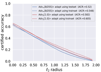
Figure 1: Certification performance on CIFAR-10 as we apply training data vs test data for adaptation in Algorithm 1. Adv${}_{\infty}[8/255]$ and Adv${}_{2}[1.0]$ respectively denote AT models, trained at $\ell_{\infty}\leq 8/255$ and $\ell_{2}\leq 1.0$ threat-boundaries.

Training versus Test images for model adaptation. Recall that adaptive BN requires a large set of diverse test images to correctly re-estimate the BN layer statistics. However, to provide certification for $\ell_{2}$-norm, we only need to adapt our model against Gaussian perturbations. Hence, unlike existing test-time adaptation-based models for covariate shift or domain adaptation problems, we can pre-select a sufficiently large and diverse set of clean images, $\mathbf{X}_{clean}$. We apply the selected level of Gaussian noise, $\sigma$ to obtain the base classifier, $f_{adapt}$ for certifying test examples, $x_{test}$. Notably, we can sample $\mathbf{X}_{clean}$ from training/validation or test sets. Since the underlying distribution of these clean images remains the same, it does not affect the certification performance. In Figure 1, we compare the performance as we randomly sample $\mathbf{X}_{clean}$ from training vs. test sets for CIFAR-10. We can see that the certification performance of AT models remains almost the same in both cases. The slight differences in their performances typically arise due to the underlying randomization of the set, $\mathbf{X}_{clean}$ and added Gaussian noise to estimate the BN parameters.

Effect on empirical robustness and benign (clean) accuracy. The main advantage of our proposed framework is that we can provide certification for AT models without affecting their state-of-the-art empirical robustness and benign accuracy. Given a test example, we first obtain the predicted class label from the original classifier, $f$ (i.e., without making any change). Next, we adapt the model to $f_{adapt}$ using appropriate $\sigma$ to certify the classification prediction using proposed Algorithm 1. Hence, we maintain the same empirical robustness and benign accuracy as reported in the existing papers (Rice et al., 2020; Madry et al., 2018).

Applicability. Our proposed “certification through adaptation" technique can be applied to any classification model, $f$ with batch-normalization layers. However, achieving high accuracy against large random Gaussian perturbations is a necessary condition: a randomized smoothing classifier, $g$ needs to consistently predict the correct class to provide higher certification guarantees at larger radii. Hence for standard non-robust DNN classifiers, we can only achieve higher $\ell_{2}$ certification guarantees at very small $\ell_{2}$ radii (see in Table 3 and Table 4). Further,we also observe that adapting the existing randomized smoothing models does not necessarily improve the overall certification performance (see Table 1 and Figure 6 in Section 4.3) In contrast, AT models with our proposed “offline" adaptation significantly improve their performance against large Gaussian perturbations, providing non-trivial certification robustness.

3.3 Proposed Auto-Noise: Appropriate Noise level for Certification

Robustness of a classification model can significantly vary at different input spaces. Hence, choosing appropriate noise-level for certifying is an important but challenging task for randomized smoothing based certification techniques. While choosing a lower noise level produces significantly lower-estimates of certified radii, over-estimation of noise may fail to provide any certification robustness for a test example. A brute-force approach to address this problem would be to evaluate the certification results on multiple noise levels and report the maximum certified $\ell_{2}$ radii. However, certification using randomized smoothing is an extremely time-consuming process: it requires to evaluate a large number of noisy samples (of cardinality $N=100,000$) to estimate $\underline{p_{A}}$ and $\overline{p_{B}}$ using Monte-Carlo sampling (Eq. 4). For example, it can take upto $110$ seconds to certify an ImageNet test example with ResNet-50 models on NVIDIA RTX 2080 Ti (Cohen et al., 2019). Notably, as we choose a smaller set of noisy samples to estimate $\underline{p_{A}}$ and $\overline{p_{B}}$, it provides significantly lower $\ell_{2}$ certified radii. Hence, existing randomized smoothing based models typically use the same Gaussian noise level as applied to train their base classifiers (Cohen et al., 2019; Salman et al., 2019a; Zhai et al., 2020; Jeong & Shin, 2020). However, we demonstrate that it significantly underestimates the certification performance of the randomized smoothing framework. Here, we present a simple but effective Auto-Noise technique to choose appropriate $\sigma$ for a given test example, $x_{test}$.

Auto-Noise technique aims to approximate the appropriate noise-level from a given set, ${\bm{\sigma}}=\{\sigma_{1},\sigma_{2},\cdots\}$. The key idea of our proposed Auto-Noise method is as follows: Although a small set of noisy examples underestimates the $\ell_{2}$ certified noise levels, it can provide a fair comparison of different noise levels for certifying $x_{test}$. We propose to use a small set of $N_{auto}$ noisy examples, $N_{auto}$ to approximately obtain the $\ell_{2}$ certification radii for different noise levels, $\sigma\in\bm{\sigma}$. We select the noise level $\sigma_{auto}$ that produces the maximum $\ell_{2}$ radius using $N_{auto}$ noisy examples, i.e.:

$$\sigma_{auto}=arg\max_{\sigma\in{\bm{\sigma}}}\quad\textsc{Certify}(g,x_{test};\sigma,N_{auto})$$ (5)

where, $g$ denotes the randomized-smoothing classifier obtained using the base classifier, $f$ (Eq. 3). For AT models, we should adapt the models, $f_{adapt}$ with noise level $\sigma$ as the base classifier.

Finally, we use $\sigma_{auto}$ for certifying $x_{test}$ with a large number of noisy samples, $N=100,000$.

Computational Overhead. In practice, the ideal choices of noise levels as ${\bm{\sigma}}$ remains reasonably small. For example, in our experiments, we select ${\bm{\sigma}}=\{0.12,0.25,0.37,0.50,0.67,0.75,0.87,1.0\}$, i.e. of cardinality=$8$ and set $N_{auto}=1,000$. Hence, we require an additional $8,000$ iterations to obtain the appropriate $\sigma$ for each test-examples, along with $100,000$ iterations to get the final certification. In other words, with very little computational overhead, we can approximate the appropriate noise levels for each test example.

Note that our Auto-Noise algorithm using a small set, $N_{auto}=1,000$ may not provide reliable estimation of the most appropriate noise-level, $\sigma$. However, as shown in Table 1, it significantly improves the certification performance for both AT models and the existing randomized smoothing based models, compared to the fixed choices of $\sigma$ (Cohen et al., 2019; Li et al., 2019). Furthermore, by using certification through adaptation along with Auto-Noise method, we can produce state-of-the-art certification performance for AT models, trained using $\ell_{2}$ bounded adversarial examples.

4 Experimental Results

Setup. We use CIFAR-10 (Krizhevsky et al., 2009) and ImageNet (Deng et al., 2009) datasets for our experiments. For CIFAR-10, we use pre-activation ResNet18 and for ImageNet, we use ResNet50 (He et al., 2016a; b). For our experiments, we train the AT models using the early stopping criteria (Rice et al., 2020). For ImageNet, we use two AT models, Adv${}_{\infty}[4/255]$ and Adv${}_{2}[3]$, learned at $\ell_{\infty}$ and $\ell_{2}$ threat models with threat boundaries of $4/255$ and $3$ respectively. For CIFAR-10, we train multiple AT models with different threat boundaries. We denote them by incorporating their corresponding threat boundaries, applied for training. For example, we denote an AT model, trained with threat boundary of $8/255$ as Adv${}_{\infty}[8/255]$.

For our comparisons, we use the standard DNN Baseline and Rand_σ=0.5 models. Baseline models are trained using clean images. Rand_σ=0.5 models are trained by augmenting random noise, sampled from $\mathcal{N}(0,\sigma^{2}I)$ with $\sigma=0.5$ Cohen et al. (2019). We also compare with the current state-of-the-art certification models, SmoothAdv for CIFAR-10 (Salman et al., 2019a). Please refer to Appendix A.2 for additional details .

(a) ImageNet						(b) CIFAR-10
Model	$\sigma=0$	$\sigma=0.25$	$\sigma=0.5$	$\sigma=0.75$		Model	$\sigma=0$	$\sigma=0.25$	$\sigma=0.5$	$\sigma=0.75$
Baseline	75.2$\pm 0.0$	11.8$\pm 0.22$	0.3$\pm 0.01$	0.1$\pm 0.0$		Baseline	95.2$\pm 0.0$	10.9$\pm 0.88$	10.6$\pm 0.76$	10.5$\pm 1.19$
+ adaptive BN	74.4$\pm 0.04$	31.0$\pm 0.27$	7.7$\pm 0.24$	2.4$\pm 0.01$		+ adaptive BN	95.0$\pm 0.57$	40.1$\pm 0.97$	22.0$\pm 0.83$	17.2$\pm 0.66$
Adv${}_{\infty}[4/255]$	62.8$\pm 0.0$	3.9$\pm 0.03$	0.4$\pm 0.01$	0.2$\pm 0.01$		Adv${}_{\infty}[8/255]$	82.1$\pm 0.0$	40.2$\pm 4.56$	16.1$\pm 7.85$	12.2$\pm 5.23$
+ adaptive BN	60.8$\pm 0.16$	53.4$\pm 0.15$	44.9$\pm 0.08$	33.7$\pm 0.28$		+ adaptive BN	81.6$\pm 0.96$	74.2$\pm 0.95$	62.4$\pm 0.64$	51.0$\pm 1.03$
Adv${}_{2}[3]$	59.8$\pm 0.0$	9.8$\pm 0.08$	0.9$\pm 0.01$	0.3$\pm 0.0$		Adv${}_{2}[1]$	81.6$\pm 0.0$	47.5$\pm 5.1$	21.5$\pm 7.79$	14.3$\pm 5.63$
+ adaptive BN	58.3$\pm 0.08$	53.7$\pm 0.14$	47.3$\pm 0.14$	39.8$\pm 0.18$		+ adaptive BN	81.8$\pm 0.7$	75.8$\pm 0.43$	64.9$\pm 0.73$	53.5$\pm 1.71$

Table 2: Top-1 accuracy of AT models significantly improve using adaptive BN under different levels of Gaussian noises (when $\sigma>0$). We randomly sample the noises and report $(mean~{}\pm~{}2\times sd)$ for five different runs.

4.1 Performance under Gaussian Noise.

We first investigate the performance of AT models as we significantly increase the Gaussian noises. As we note in Section 3.1, it is a necessary condition to provide non-trivial robustness certification at larger $\ell_{2}$ radii. In Table 2, we present a comparative performance for Baseline, Adv_∞, and Adv₂ models for both ImageNet and CIFAR-10 datasets. We can see that the classification performance of all these models sharply degrades under large Gaussian noises in standard inference settings. However, we can improve these performances by adapting them under the same level of Gaussian noises using adaptive BN techniques. In particular, we observe that AT models achieve significantly higher performance gain using adaptive BN than the non-robust, Baseline models under Gaussian noise levels. For example, at $\sigma=0.5$, Baseline, Adv${}_{2}[3]$ and Adv${}_{\infty}[4/255]$ respectively achieve top-1 accuracy of $0.3\%$, $0.4\%$, and $0.9\%$ for ImageNet without using BN adaptation (Table 2 (a)). However, adaptive BN for Adv${}_{2}[3]$ and Adv${}_{\infty}[4/255]$ significantly improves the top-1 accuracy to $47.3\%$ and $44.9\%$ respectively. In contrast, the baseline model only achieves $7.7\%$ accuracy. We also observe similar results for CIFAR-10 in Table 2 (b).

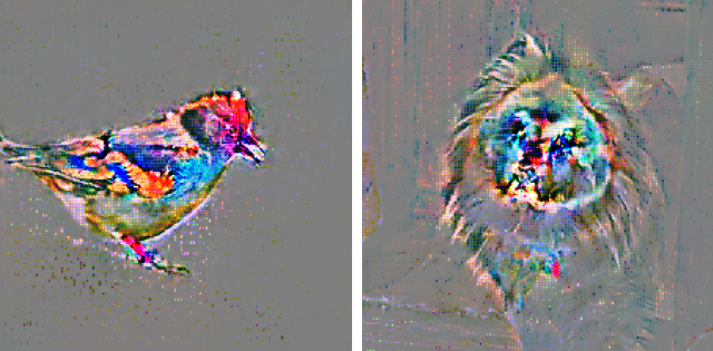
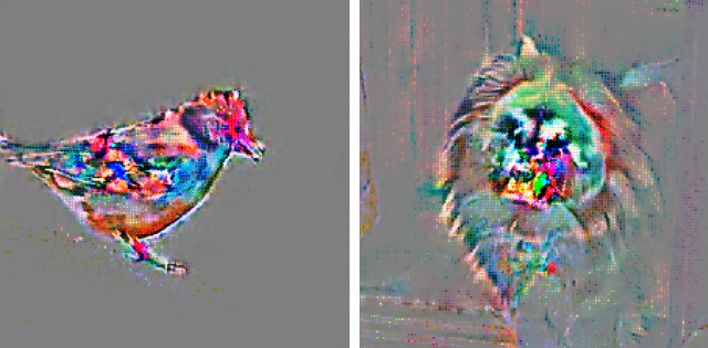
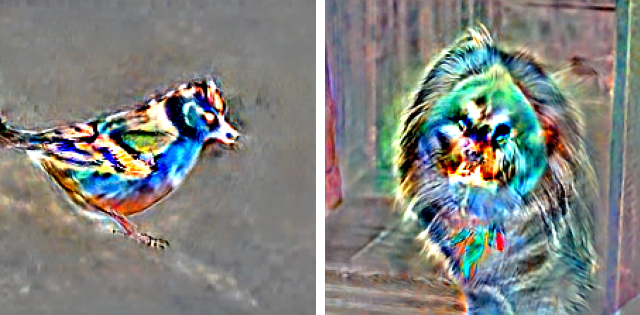
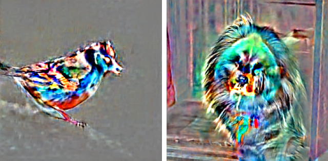
(a) $\sigma=0$ (Clean)

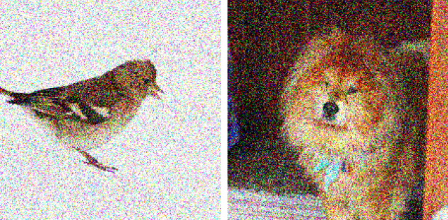
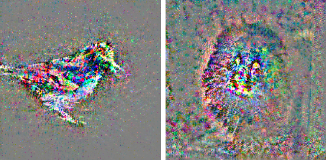
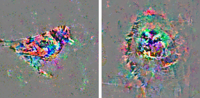
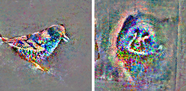
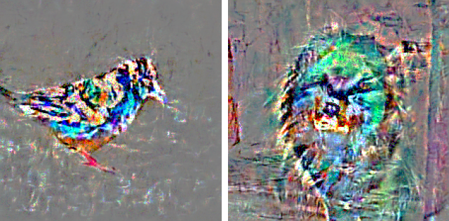
(b) $\sigma=0.25$

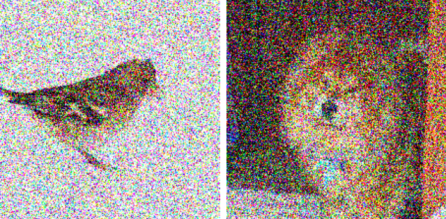
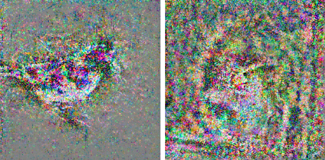
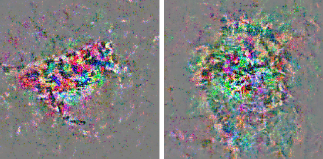
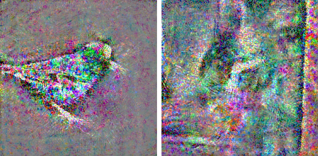
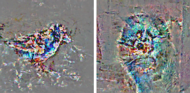
(c) $\sigma=0.5$

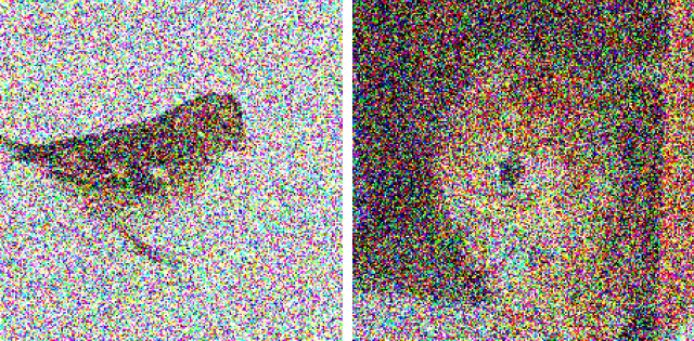
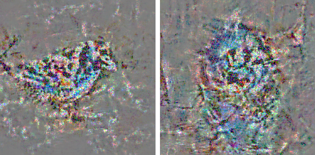
(d) $\sigma=0.75$

Figure 2: Visualizing loss-gradients produced by AT models as we apply different levels of Gaussian noises.

Adaptive BN for AT models correctly extracts robust features under Gaussian noises. In Figure 2, we further investigate the performance of AT models by visualizing the loss gradients of individual pixels of an image as we increase the noise level , $\sigma$. Loss-gradients reflect the most relevant input pixels for classification predictions. Here, we scale, translate and clip the loss-gradient values without using any sophisticated techniques (as in Tsipras et al. (2019)). At $\sigma=0$ (i.e., for clean images), the loss-gradients from AT models align properly with perceptually relevant features (as observed previously (Tsipras et al., 2019; Etmann et al., 2019)). However, as we choose higher noise using $\sigma$=$0.5$ and $\sigma$=$0.75$, the overall loss gradients become noisier. Specifically, we can see that AT models without BN adaptation produce larger gradient values (i.e., greater importance) even for background pixels. In contrast, AT models with BN adaptation using Gaussian noises allows to correctly extract perceptually relevant features from the object of interest, suppressing the gradients for background (refer to Figure 2(c) and Figure 2(d)). In other words, it allows us to extract the required semantic information for correct classifications. Also, it is interesting to note that Adv₂ produces significantly more human-aligned loss gradients compared to Adv_∞. This behavior is also reflected in their classification performance in Table 2 and certification robustness in Table 1. We can see that Adv₂ overall produces better performance compared to Adv_∞. These results indicate that we can achieve non-trivial certification results by appropriately adapting the AT models, as demonstrated in the following sections.

4.2 Certified Robustness for AT models

We now present the $\ell_{2}$ certification results using the randomized smoothing framework as the backbone, as proposed in our Algorithm 1. We certify the test images with $99.9\%$ probability. We estimate the class-label probabilities of $g$ (Equation 4) using $100,000$ noisy samples, as in (Cohen et al., 2019; Salman et al., 2019a). We use the full test-set of $10,000$ images for CIFAR-10 and a sub-sample of $500$ test images for ImageNet.

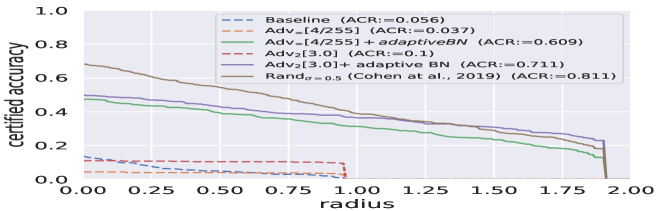
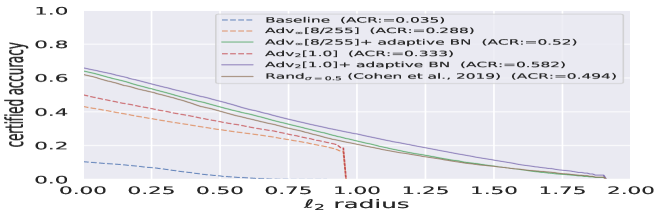
Figure 3: Certification through adaptation produces non-trivial certified robustness at various $\ell_{2}$ radii for both (Left) ImageNet and (Right) CIFAR-10 datasets.

Non-trivial certification for AT models. In Figure 3, we first demonstrate that AT models can achieve non-trivial $\ell_{2}$ certified robustness using our proposed certification through adaptation technique for both ImageNet and CIFAR-10 datasets. Here, we use Adv${}_{\infty}[4/255]$ and Adv${}_{2}[3]$ for ImageNet and Adv${}_{\infty}[8/255]$ and Adv${}_{2}[1]$ for CIFAR-10. We apply fixed noise levels of $\sigma=0.5$ to certify all test examples using proposed Algorithm 1. Here, we compare with the certification results of the Baseline, Adv_∞ and Adv₂ models at $\sigma=0.25$ in the standard settings (i.e., without adapting these models). We can see a significant boost of $\ell_{2}$ certification results for both Adv_∞ and Adv₂ models using our proposed framework. Further, Adv₂ models consistently achieve better certification performance compared to Adv_∞. We also compare with Rand_σ=0.5 models at fixed $\sigma=0.5$, as in Cohen et al. (2019). For CIFAR-10, both Adv${}_{\infty}[8/255]$ and Adv${}_{2}[1]$ outperform the Rand_σ=0.5 models (Cohen et al., 2019). Furthermore, for ImageNet, Adv${}_{2}[3]$ achieves better certified accuracy compared to Rand_σ=0.5 beyond $\ell_{2}$-radii of $1.5$. Please refer to Table 3 and 4 (Appendix) for detailed comparisons of different models, trained using different specifications.

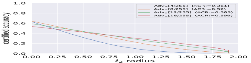
(a)

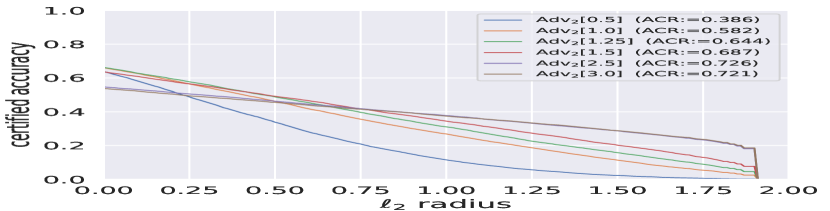
(b)

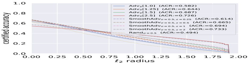
(c)

Figure 4: CIFAR-10: AT models, trained using larger threat boundaries, produces better certification results for higher $\ell_{2}$ radii. Here, we apply our proposed certification through adaptation with fixed noise-level $\sigma=0.5$. (c) Comparison of Adv₂ models with SmoothAdv (Salman et al., 2019a), trained and certified using $\sigma=0.5$.

Larger Threat Boundary for Better Certification. Learning AT models at a higher threat boundary produces better certified robustness at higher $\ell_{2}$ radii. Figure 4(a) and 4(b) demonstrate this phenomena for CIFAR-10 on both Adv_∞ and Adv₂ models respectively .

Figure 4(c) also compares the certified accuracy of Adv₂ models with the existing state-of-the-art SmoothAdv models (Salman et al., 2019a). SmoothAdv utilizes adversarial training using an adaptive attack with an $\ell_{2}$ threat boundary of $\epsilon$ and Gaussian noises, $\mathcal{N}(0,\sigma^{2}I)$ (See details in Appendix A.2). We set the noise to $\sigma=0.5$ and vary $\epsilon$ for their training to compare with different SmoothAdv models in Figure 4(c). As we can see that by adapting Adv₂ models at $\sigma=0.5$ using our proposed Algorithm 1, we can already achieve similar performance as SmoothAdv. Next, we demonstrate that our proposed Auto-Noise technique further improves the performance of both AT models and existing randomized smoothing based models.

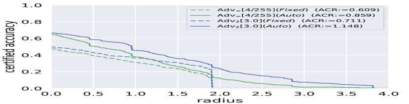
(a) ImageNet

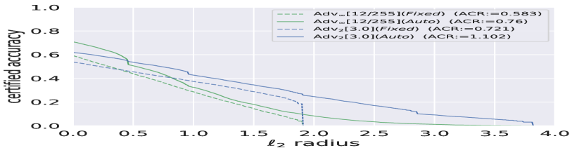
(b) CIFAR-10

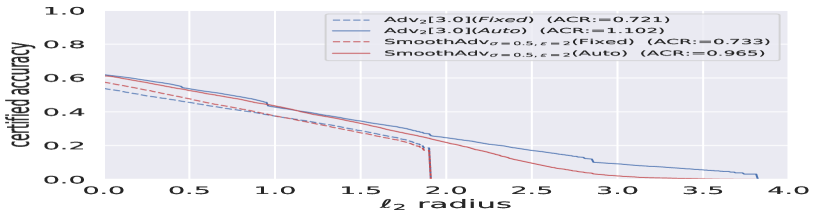
(c) SmoothAdv vs Adv₂ (CIFAR-10)

Figure 5: Auto-Noise (denoted as "auto") vs. fixed noise at $\sigma=0.5$ (denoted as "fixed") for $\ell_{2}$ certification on (a) ImageNet and (b) CIFAR-10 datasets for AT models. (c) SmoothAdv vs Adv₂ models for CIFAR-10 using Auto-Noise technique. Here, we only present the results with the best ACR scores.

4.3 Auto-Noise: Flexibility of choosing appropriate $\sigma$ for certification.

In Table 2, we can see that the classification models remain robust only for a few test examples under higher Gaussian noise. It suggests that the optimal noise levels for certifying different test examples may vary significantly, indicating the importance of our proposed Auto-Noise technique.

Auto-Noise for AT models. Figure 5(a) and 5(b) present the certification performance of AT models as we apply both certification through adaptation (Algorithm 1) and Auto-Noise technique for for ImageNet and CIFAR-10 datasets respectively. We compare their performance by certifying using a fixed noise level, $\sigma=0.5$. We can see that the Auto-Noise technique can significantly improve the performance to achieve $1.148$ and $1.102$ ACR scores for the best AT models on ImageNet and CIFAR-10 datasets. Figure 5(c) demonstrates that the Auto-Noise technique also improves the performance of the best SmoothAdv model to an ACR score of $0.965$ for CIFAR-10. However, our Certification through Adaptation together with Auto-Noise technique for Adv${}_{2}[3]$ model outperforms the best SmoothAdv model for CIFAR-10.

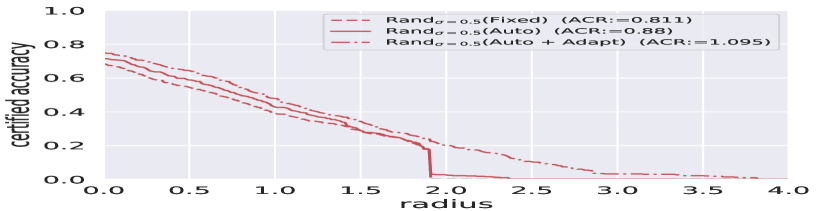
(a) Rand_σ=0.5 (ImageNet)

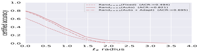
(b) Rand_σ=0.5 (CIFAR-10)

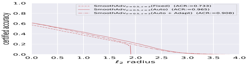
(c) SmoothAdv (CIFAR-10)

Figure 6: Effect of adaptation and Auto-Noise technique for existing randomized smoothing based models.

Certification through Adaptation along with Auto-Noise for existing models. In Figure 6, we compare the performance of existing randomized smoothing based models as we adapt their base models using Algorithm 1 followed by Auto-Noise technique. We can see in Figure 6(a) that incorporating adaptation using Algorithm 1 improves the Rand_σ=0.5 model to achieve ACR score of $1.095$ on ImageNet dataset. In contrast, the certification performance for both Rand_σ=0.5 and SmoothAdv models degrades for CIFAR-10 datasets (Figure 6(b) and Figure 6(c)). Hence, we do not include these models in Figure 5 (c) to compare with AT models.

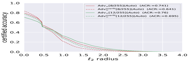
(a) Adv_∞ models

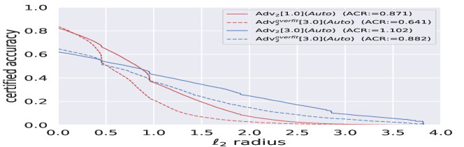
(b) Adv₂ models

Figure 7: CIFAR-10: Certification performance degrades for over-fitted AT models when trained without applying early-stopping criteria (Rice et al., 2020). The over-fitted models are denoted as Adv^overfit.

4.4 Over-fitted AT models degrades certification

Rice et al. (2020) demonstrate that AT models overfit when trained without early stopping criteria. It degrades their empirical robustness against adversarial attacks. Figure 7 compares with the certification results of such overfitted AT models, denoted as Adv^overfit. We observe that Adv^overfit models also degrade the certified robustness compared to their corresponding AT models, trained with early stopping criteria. In particular, the difference in their certification performance is more prominent at higher $\ell_{2}$ radii. Hence, these results as well as our results in Figure 5 indicate that empirical and certified robustness are closely related. In particular, improving the empirical robustness for a model also allows to provide better certified robustness.

5 Conclusion

We propose a novel certification through adaptation algorithm that transforms the AT models into a randomized smoothing classifier to provide certified robustness for $\ell_{2}$ norm. We also propose Auto-Noise to efficiently approximate the appropriate noise levels to certify different test examples. Empirically we improve the performance of both AT models and existing randomized smoothing-based models on CIFAR-10 and ImageNet datasets using the Auto-Noise technique. Further, our Certification through Adaptation together with Auto-Noise technique significantly improves the ACR scores using AT models. Notably, our framework does not affect the empirical robustness or benign accuracy of an AT model to provide these non-trivial $\ell_{2}$ certification results. Hence, our paper is a step towards bridging the gap between current research of empirical and certified robustness against adversarial examples.

Broader Impact Statement

Improving empirical robustness against adversarial examples along with certification guarantees is an important problem to enhance the reliability of a DNN model for sensitive real-world applications. However, the current state-of-the-art defense methods against adversarial examples typically focus on improving either empirical or certified robustness. In this paper, we aim to bridge this gap by significantly improving the certification performance of AT models without affecting the benign accuracy or reducing their state-of-the-art empirical robustness.

Appendix A Appendix

A.1 Detailed Certification results for different models using proposed method

ImageNet
Model	Noise-level	$\ell_{2}$ Radius
		0.0	0.25	0.5	0.75	1.0	1.25	1.5	1.75	2.0	2.25	2.5	2.75	3.0	ACR
Baseline	$\sigma=$ 0.25	13.6	7.8	4.8	3.0	0.0	0.0	0.0	0.0	0.0	0.0	0.0	0.0	0.0	0.055
Baseline	Auto-Noise	52.4	36.8	5.0	3.2	0.6	0.6	0.4	0.4	0.4	0.4	0.4	0.4	0.4	0.194
Baseline + Adaptation	Auto-Noise	57.4	25.8	4.6	1.8	0.4	0.2	0.0	0.0	0.0	0.0	0.0	0.0	0.0	0.15
Adv${}_{\infty}[4/255]$	Auto-Noise	34.6	31.2	4.0	3.8	0.6	0.6	0.4	0.4	0.2	0.2	0.0	0.0	0.0	0.169
Adv${}_{\infty}[4/255]$ + Adaptation	$\sigma=$ 0.5	47.4	43.6	39.4	35.8	31.4	27.6	23.4	18.2	0.0	0.0	0.0	0.0	0.0	0.609
Adv${}_{\infty}[4/255]$ + Adaptation	Auto-Noise	65.6	59.4	50.6	46.6	38.0	33.2	26.2	20.8	12.0	8.6	6.0	4.0	1.6	0.859
Adv${}_{2}[3.0]$	Auto-Noise	44.0	41.6	11.8	11.2	2.8	2.6	0.4	0.4	0.0	0.0	0.0	0.0	0.0	0.261
Adv${}_{2}[3.0]$ + Adaptation	$\sigma=$ 0.5	50.2	47.0	43.0	39.0	36.4	32.8	30.8	27.0	0.0	0.0	0.0	0.0	0.0	0.711
Adv${}_{2}[3.0]$ + Adaptation	Auto-Noise	66.6	63.8	58.6	55.4	45.6	41.0	35.8	32.4	23.6	18.6	15.0	12.8	7.4	1.148
Randσ=0.5	$\sigma=$ 0.50	68.2	60.8	54.4	47.8	38.8	33.8	28.6	23.4	0.0	0.0	0.0	0.0	0.0	0.811
Randσ=0.5	Auto-Noise	71.4	65.6	58.8	51.4	42.8	37.0	28.8	23.8	2.6	1.6	0.2	0.2	0.2	0.88
Randσ=0.5 + Adaptation	Auto-Noise	74.8	69.8	64.4	56.6	47.8	40.0	34.4	27.4	20.2	15.8	10.4	6.4	3.2	1.095

Table 3: ImageNet: Certified top-1 accuracy at various $\ell_{2}$ radii as we vary $\sigma$ for BN adaptation and certification along with average certified radii (ACR). We use ResNet50 for ImageNet.

ImageNet
Model	Noise-level	$\ell_{2}$ Radius
		0.0	0.25	0.5	0.75	1.0	1.25	1.5	1.75	2.0	2.25	2.5	2.75	3.0	ACR
Baseline	$\sigma=$ 0.25	10.49	6.96	2.04	0.09	0.0	0.0	0.0	0.0	0.0	0.0	0.0	0.0	0.0	0.035
Baseline	Auto-Noise	33.57	18.56	10.25	4.44	0.83	0.07	0.01	0.0	0.0	0.0	0.0	0.0	0.0	0.124
Baseline + Adaptation	Auto-Noise	59.64	21.66	7.81	3.97	1.28	0.36	0.07	0.0	0.0	0.0	0.0	0.0	0.0	0.154
Adv${}_{\infty}[4/255]$	Auto-Noise	73.71	63.04	28.75	23.91	17.96	14.19	10.12	7.08	4.99	4.14	3.24	2.49	1.84	0.57
Adv${}_{\infty}[4/255]$ + Adaptation	$\sigma=0.5$	63.23	47.34	31.83	18.78	9.98	4.44	1.62	0.28	0.0	0.0	0.0	0.0	0.0	0.361
Adv${}_{\infty}[4/255]$ + Adaptation	Auto-Noise	85.53	76.02	49.42	36.23	21.05	13.4	8.7	5.58	3.15	1.69	0.66	0.19	0.07	0.654
Adv${}_{\infty}[8/255]$	Auto-Noise	74.46	66.57	36.32	30.15	18.87	13.71	8.7	5.29	2.89	1.88	1.17	0.75	0.46	0.578
Adv${}_{\infty}[8/255]$ + Adaptation	$\sigma=0.5$	64.2	53.65	42.91	32.58	22.68	14.24	7.88	2.94	0.0	0.0	0.0	0.0	0.0	0.52
Adv${}_{\infty}[8/255]$ + Adaptation	Auto-Noise	79.69	71.78	53.76	43.61	29.68	20.87	14.04	9.08	5.53	3.33	1.71	0.81	0.35	0.741
Adv${}_{\infty}[12/255]$	Auto-Noise	69.46	63.12	35.73	30.63	17.54	14.78	10.27	9.16	8.01	7.2	6.21	5.31	3.78	0.649
Adv${}_{\infty}[12/255]$ + Adaptation	$\sigma=0.5$	59.19	51.53	43.94	36.41	28.69	21.25	14.53	8.03	0.0	0.0	0.0	0.0	0.0	0.583
Adv${}_{\infty}[12/255]$ + Adaptation	Auto-Noise	70.75	64.54	50.63	43.38	32.5	24.43	18.05	12.2	8.31	5.37	3.36	1.96	1.23	0.76
Adv${}_{\infty}[16/255]$	Auto-Noise	58.47	53.41	31.48	26.76	16.68	14.04	10.89	9.17	7.42	5.62	3.81	2.43	1.53	0.55
Adv${}_{\infty}[16/255]$ + Adaptation	$\sigma=0.5$	53.8	48.07	42.51	36.54	30.55	24.68	18.49	12.11	0.0	0.0	0.0	0.0	0.0	0.599
Adv${}_{\infty}[16/255]$ + Adaptation	Auto-Noise	61.07	56.01	45.76	40.29	31.6	24.53	18.73	14.23	10.39	7.37	5.05	3.36	2.13	0.731
Adv${}_{2}[0.5]$	Auto-Noise	71.6	61.2	22.17	17.64	12.26	10.97	10.17	9.76	9.48	9.12	8.53	7.52	6.61	0.603
Adv${}_{2}[0.5]$ + Adaptation	$\sigma=0.5$	63.77	48.81	33.82	20.95	11.5	5.64	2.29	0.62	0.0	0.0	0.0	0.0	0.0	0.386
Adv${}_{2}[0.5]$ + Adaptation	Auto-Noise	86.26	77.52	61.25	46.44	23.42	16.22	11.55	9.2	7.62	6.47	5.07	3.81	2.51	0.796
Adv${}_{2}[1.0]$	Auto-Noise	81.08	74.0	43.82	34.77	17.25	11.15	6.19	3.68	1.76	1.02	0.52	0.27	0.15	0.608
Adv${}_{2}[1.0]$ + Adaptation	$\sigma=0.5$	66.05	56.45	46.24	35.6	26.89	18.73	11.37	5.41	0.0	0.0	0.0	0.0	0.0	0.582
Adv${}_{2}[1.0]$ + Adaptation	Auto-Noise	82.34	75.38	64.53	53.8	36.04	27.55	19.53	12.61	7.29	4.33	2.39	1.21	0.67	0.871
Adv${}_{2}[1.25]$	Auto-Noise	78.32	72.56	44.86	39.13	25.98	21.02	16.31	12.17	8.18	5.18	2.25	1.25	0.66	0.741
Adv${}_{2}[1.25]$ + Adaptation	$\sigma=0.5$	66.22	57.73	48.8	39.64	31.07	22.61	15.82	8.96	0.0	0.0	0.0	0.0	0.0	0.644
Adv${}_{2}[1.25]$ + Adaptation	Auto-Noise	80.52	74.25	64.95	56.56	40.81	32.71	24.96	17.87	11.5	8.07	5.88	4.05	2.59	0.972
Adv${}_{2}[1.5]$	Auto-Noise	75.26	69.75	48.42	41.73	26.44	20.82	14.12	10.14	6.87	4.75	3.02	1.81	0.87	0.733
Adv${}_{2}[1.5]$ + Adaptation	$\sigma=0.5$	63.67	56.55	49.19	41.72	34.47	27.36	20.23	12.98	0.0	0.0	0.0	0.0	0.0	0.687
Adv${}_{2}[1.5]$ + Adaptation	Auto-Noise	76.22	70.47	62.39	55.91	42.45	35.79	29.01	21.71	14.23	10.04	6.51	4.07	2.29	0.99
Adv${}_{2}[2.5]$	Auto-Noise	61.2	57.42	42.26	38.0	26.56	21.41	14.21	10.34	7.33	4.96	3.24	2.06	1.07	0.662
Adv${}_{2}[2.5]$ + Adaptation	$\sigma=0.5$	54.73	50.53	46.26	41.84	37.74	33.2	28.69	23.34	0.0	0.0	0.0	0.0	0.0	0.726
Adv${}_{2}[2.5]$ + Adaptation	Auto-Noise	63.36	59.53	54.68	50.3	42.95	38.62	33.97	29.42	23.03	19.22	15.3	11.34	7.51	1.073
Adv${}_{2}[3.0]$	Auto-Noise	64.45	60.57	45.73	41.06	28.48	22.92	15.1	10.77	7.23	4.8	2.77	1.67	1.1	0.702
Adv${}_{2}[3.0]$ + Adaptation	$\sigma=0.5$	53.75	49.41	45.57	41.52	37.43	33.37	28.82	23.65	0.0	0.0	0.0	0.0	0.0	0.721
Adv${}_{2}[3.0]$ + Adaptation	Auto-Noise	61.96	58.58	53.64	49.67	42.76	38.69	34.54	30.36	24.65	20.77	17.09	13.66	9.18	1.102
Randσ=0.5	$\sigma=0.5$	62.13	51.68	40.38	30.25	20.81	13.36	7.71	3.38	0.0	0.0	0.0	0.0	0.0	0.494
Randσ=0.5	Auto-Noise	79.48	71.75	60.23	48.72	35.97	25.16	15.09	10.13	6.98	5.58	4.18	2.94	1.76	0.821
Randσ=0.5 + Adaptation	Auto-Noise	78.27	69.51	57.16	44.73	31.19	19.27	10.4	4.25	1.65	0.57	0.14	0.01	0.0	0.695
SmoothAdvσ=0.5,ϵ=0.25	$\sigma=0.5$	67.35	57.8	47.63	37.41	27.88	20.33	13.53	8.03	0.0	0.0	0.0	0.0	0.0	0.614
SmoothAdvσ=0.5,ϵ=0.25	Auto-Noise	72.88	65.23	55.25	44.87	34.93	24.79	16.44	9.17	4.92	1.91	0.73	0.21	0.07	0.737
SmoothAdvσ=0.5,ϵ=0.25 + Adaptation	Auto-Noise	74.45	65.68	54.28	42.59	31.76	21.61	13.19	7.16	3.41	1.43	0.52	0.16	0.05	0.697
SmoothAdvσ=0.5,ϵ=0.5	$\sigma=0.5$	67.21	58.82	49.68	40.35	31.93	24.18	17.05	10.57	0.0	0.0	0.0	0.0	0.0	0.665
SmoothAdvσ=0.5,ϵ=0.5	Auto-Noise	71.85	65.28	56.41	48.2	39.47	29.82	21.44	13.55	7.54	3.45	1.35	0.41	0.12	0.807
SmoothAdvσ=0.5,ϵ=0.5 + Adaptation	Auto-Noise	73.54	66.14	56.81	47.04	37.2	26.99	18.46	10.78	5.67	2.6	1.0	0.44	0.13	0.773
SmoothAdvσ=0.5,ϵ=1.0	$\sigma=0.5$	63.95	56.53	49.53	41.38	34.63	27.81	21.22	14.41	0.0	0.0	0.0	0.0	0.0	0.694
SmoothAdvσ=0.5,ϵ=1.0	Auto-Noise	67.91	62.28	55.36	48.41	41.14	33.57	26.27	18.42	11.87	6.1	2.64	0.95	0.32	0.854
SmoothAdvσ=0.5,ϵ=1.0 + Adaptation	Auto-Noise	69.6	63.04	55.52	47.65	38.93	30.7	22.57	15.34	9.21	4.51	2.02	0.9	0.33	0.813
SmoothAdvσ=0.5,ϵ=2.0	$\sigma=0.5$	57.59	52.82	47.67	42.68	37.55	32.64	27.52	22.42	0.0	0.0	0.0	0.0	0.0	0.733
SmoothAdvσ=0.5,ϵ=2.0	Auto-Noise	61.27	57.27	52.52	48.17	43.49	38.02	33.15	27.47	21.86	15.81	9.5	4.97	2.01	0.965
SmoothAdvσ=0.5,ϵ=2.0 + Adaptation	Auto-Noise	61.23	56.9	51.33	46.44	41.05	35.65	30.11	24.35	18.48	12.8	7.76	4.27	2.3	0.908

Table 4: CIFAR-10: Certified top-1 accuracy at various $\ell_{2}$ radii as we vary $\sigma$ for test-time BN adaptation along with average certified radii (ACR) for individual settings.

A.2 Implementation Details

We present our experimental results on CIFAR-10 (Krizhevsky et al., 2009) and ImageNet (Deng et al., 2009) datasets. The descriptions of different models and training hyper-parameters are provided in the following:

A.2.1 CIFAR-10.

We use pre-activation ResNet18 architecture (He et al., 2016b) for our experiments on CIFAR-10. We apply the SGD optimizer with a batch size of $128$. We execute a total of $200$ training epochs and apply a step-wise learning rate decay set initially at $0.1$ and divided by $10$ at $100$ and $150$ epochs, and weight decay $5\times 10^{-4}$.

AT models (Madry et al., 2018; Rice et al., 2020): Unless and otherwise specified, our AT models are learned using early stopping criteria as described in (Rice et al., 2020). We learn several AT models with different threat boundaries for our experiments. We denote them by specifying their corresponding threat model and threat boundaries. For example, Adv${}_{2}[1.5]$ denotes an AT model that is learned using PGD adversary with $\ell_{2}$ threat model and a threat boundary of $\epsilon=1.5$, along with early-stopping criteria (Rice et al., 2020). We also learn AT models without using early-stopping criteria, as in (Madry et al., 2018) for our comparison in Figure 7. These models are denoted as Adv^overfit.

We use projected gradient descent (PGD) adversarial attack (Madry et al., 2018) to train these AT models as follows: For Adv_∞, we use $10$ iterations and an $\ell_{\infty}$ step size of $\epsilon/4$. For Adv₂, we use $10$ iterations and an $\ell_{2}$ step size of $\epsilon/8.5$. This is the same experimental setup as in (Rice et al., 2020)). We choose a small set of $1,000$ images from the CIFAR-10 test set for our validation. We apply the PGD attack with the same hyper-parameters for our validation during training. We save the best model using the early-stopping criteria (Rice et al., 2020).

Randomized smoothing model by Cohen et al. (2019): We also train Rand_σ=0.5 by training with augmented random noise, sampled from an isotropic Gaussian distribution $\mathcal{N}(0,\sigma^{2}I)$ with $\sigma=0.5$. Here, we keep the same model architecture, learning rates, batch sizes, and other hyper-parameters as used to learn the AT models.

Randomized smoothing model by Salman et al. (2019a): We also compare with the state-of-the-art certification models, called ‘SmoothAdv’, by Salman et al. (2019a) for our experiments on $\ell_{2}$ certification We train the SmoothAdv models by choosing random noise vectors followed by an adaptive adversarial attack with specified $\ell_{2}$ threat boundary of $\epsilon$ at each iteration. The noise vectors are sampled from an isotropic Gaussian distribution $\mathcal{N}(0,\sigma^{2}I)$.

We note that the training hyper-parameter $\epsilon$ has the most significant impact on the certification curve for a SmoothAdv model (please refer to Table 7-15 of (Salman et al., 2019a) for more details). For our experiments, we train $4$ different SmoothAdv models with $\epsilon=\{0.25,0.5,1,2\}$ and $\sigma=0.5$ using adaptive PGD attack with $10$ steps. We denote them as SmoothAdv_{σ=0.5,ϵ=0.25}, SmoothAdv_{σ=0.5,ϵ=0.5}, SmoothAdv_σ=0.5,ϵ=1 and SmoothAdv_σ=0.5,ϵ=2 respectively. We use the same training set-up and other hyper-parameters as specified in their Github: https://github.com/Hadisalman/smoothing-adversarial.

A.2.2 ImageNet.

We use ResNet50 architecture (He et al., 2016a) for ImageNet. We obtain the Baseline and Rand_σ=0.5 models from (Cohen et al., 2019). These models are trained using Gaussian augmented noises, sampled from isotropic Gaussian distribution $\mathcal{N}(0,\sigma^{2}I)$ with $\sigma=0.0$ (i.e., no noise) and $\sigma=0.5$ respectively.

The AT models i.e., Adv${}_{\infty}[4/255]$ and Adv${}_{2}[3.0]$ are learned for $\ell_{\infty}$ and $\ell_{2}$ threat models with threat boundary of $4/255$ and $3$, respectively. We use the publicly available models provided by Rice et al. (2020) . These models are fine-tuned using PGD-based adversarial training with early stopping criteria, originally provided by Engstrom et al. (2019) .

We resize the input images to $256\times 265$ pixels and crop $224\times 224$ pixels from the center. For our experiments on certification, we use a set of $500$ test images by choosing at most $1$ sample for each class.

A.3 Choice of Adaptive BN hyper-parameters

BN adaptation technique is controlled by two hyper-parameters, i.e., the test batch-size and momentum ($\rho$) (see Equation 2) to update the statistics of the batch-normalization layers. Assuming that the test images are obtained independently from the same test distribution, we can efficiently compute the BN statistics from these images. The hyper-parameter $\rho\in[0,1]$ controls the tread-off between pre-computed training statistics and test statistics. We can obtain a better estimation of the test distribution from a large test batch. Hence, we can choose a higher value of $\rho$.

Here, we compare the top-1 test accuracy of AT models under Gaussian augmented noise with $\sigma=0.5$ for different choices of $\rho$ and the batch size. We skip the standard baseline models from our analysis and refer to the previous works (Schneider et al., 2020; Nado et al., 2020) that analyzed the effects of these hyper-parameters for the standard baseline DNN classifiers.

(a) ImageNet				(b) CIFAR-10
$\rho$	Adv∞	Adv2		$\rho$	Adv∞	Adv2
0.0 (No adaptation)	0.4$\pm 0.01$	0.9$\pm 0.01$		0.0 (No adaptation)	16.1$\pm 7.85$	21.5$\pm 7.79$
0.1	2.1$\pm 0.04$	7.7$\pm 0.09$		0.1	45.1$\pm 0.49$	46.9$\pm 0.48$
0.3	20.6$\pm 0.16$	36.6$\pm 0.09$		0.3	59.2$\pm 0.42$	60.8$\pm 0.33$
0.5	41.1$\pm 0.09$	45.5$\pm 0.13$		0.5	62.4$\pm 0.27$	64.4$\pm 0.6$
0.7	43.5$\pm 0.14$	46.7$\pm 0.13$		0.7	62.8$\pm 0.52$	64.9$\pm 0.31$
0.9	44.2$\pm 0.12$	46.8$\pm 0.13$		0.9	62.8$\pm 0.71$	64.9$\pm 0.31$
1.0 (Full adaptation)	44.8$\pm 0.13$	47.2$\pm 0.14$		1.0 (Full adaptation)	62.4$\pm 0.64$	64.9$\pm 0.73$

Table 5: Top-1 accuracy using fixed test batch-size $=512$ for AT models under Gaussian augmented noise with $\sigma=0.5$ for different choices of momentum, $\rho$ during inference. We randomly shuffle the test images to report ($mean+2\times sd$) of $5$ different runs.

Momentum ($\rho$).

We first investigate the effect of momentum ($\rho$) as we choose a large batch size of $512$. In Table 5, we present the performance of AT models for different values of $\rho$. Recall that, $\rho=1$ denotes full adaptation (Equation 2). Here, we completely ignore the training statistics and recompute the BN statistics using the test batches. In contrast, $\rho=0$ represents no adaptation, i.e., the same as the standard ‘deterministic’ inference setup. In this case, we use the previously computed BN statistics obtained during training.

We observe that for ImageNet (Table 5 [Left]) the performance started converging at $\rho=0.7$. For CIFAR-10 (Table 5 [Right]), the convergence started even earlier at $\rho=0.5$.

(a) ImageNet				(b) CIFAR-10
Batch Size	Adv∞	Adv2		Batch Size	Adv∞	Adv2
w/o BN adapt	0.4$\pm 0.01$	0.9$\pm 0.01$		w/o BN adapt	16.1$\pm 7.85$	21.5$\pm 7.79$
8	11.5$\pm 0.22$	9.1$\pm 0.15$		8	57.2$\pm 1.23$	59.5$\pm 0.38$
16	28.1$\pm 0.22$	26.7$\pm 0.14$		16	60.2$\pm 0.79$	62.3$\pm 0.87$
32	37.1$\pm 0.24$	37.6$\pm 0.2$		32	61.5$\pm 0.46$	63.6$\pm 0.55$
64	41.4$\pm 0.26$	42.9$\pm 0.12$		64	62.3$\pm 0.5$	64.0$\pm 0.38$
128	43.3$\pm 0.15$	45.4$\pm 0.13$		128	62.7$\pm 0.68$	64.4$\pm 0.53$
256	44.4$\pm 0.21$	46.7$\pm 0.07$		256	62.7$\pm 0.68$	64.9$\pm 0.48$
512	44.8$\pm 0.13$	47.2$\pm 0.14$		512	62.4$\pm 0.64$	64.9$\pm 0.73$

Table 6: Top-1 accuracy using fixed $\rho=1$ for AT models under Gaussian augmented noise with $\sigma=0.5$ for different size of test batches during inference. We randomly shuffle the test images to report ($mean+2\times s.d.$) of $5$ different runs.

Batch Size.

Next, we investigate the minimum size of the test batches to choose $\rho=1$ (i.e., full-adaptation). In Table 6, we fix $\rho=1$ and vary the test batch sizes as we evaluate these AT models. We observe that the performance of these models started improving even when we are using the test batches of size $8$. The performance further improves as we choose larger sizes of test batches. We can see that their performance started converging as we choose the test batches of size $64$ for ImageNet. On the other hand, the convergence started much earlier for CIFAR-10.

A.4 Performance against different corruptions

We mainly focus on $\ell_{2}$ certification using Gaussian noise in this paper. However, we note that randomized smoothing techniques have been also applied to provide certifications for other perturbation types as well (e.g., random uniform noise for $\ell_{1}$ norm (Yang et al., 2020)). Consequently, we can apply our proposed Algorithm 1 to adapt an AT model for any given perturbation types without any additional training for different applications.

Further, Hendrycks & Dietterich (2019) recently introduced ImageNet-C and CIFAR10-C datasets by algorithmically generated random corruptions from noise, blur, weather, and digital categories with $5$ different severity levels for each corruption. Several recent works demonstrated that adaptive BN techniques can significantly improve the performance of any classifier (including AT models) against different random corruptions. Further, – also demonstrated the effectiveness of AT models even without applying any adaptation. Hence, our proposed certification framework for AT models is a step forward towards further improving the reliability of sensitive real-world applications.

References

- Athalye et al. (2018) Anish Athalye, Nicholas Carlini, and David Wagner. Obfuscated gradients give a false sense of security: Circumventing defenses to adversarial examples. In ICML, 2018.
- Benz et al. (2021a) Philipp Benz, Chaoning Zhang, Adil Karjauv, and In So Kweon. Revisiting batch normalization for improving corruption robustness. In WACV, 2021a.
- Benz et al. (2021b) Philipp Benz, Chaoning Zhang, and In So Kweon. Batch normalization increases adversarial vulnerability and decreases adversarial transferability: A non-robust feature perspective. In ICCV, 2021b.
- Bunel et al. (2018) Rudy Bunel, Ilker Turkaslan, Philip HS Torr, Pushmeet Kohli, and M Pawan Kumar. A unified view of piecewise linear neural network verification. NeurIPS, 2018.
- Cao & Gong (2017) Xiaoyu Cao and Neil Zhenqiang Gong. Mitigating evasion attacks to deep neural networks via region-based classification. In ACSAC, 2017.
- Cariucci et al. (2017) Fabio Maria Cariucci, Lorenzo Porzi, Barbara Caputo, Elisa Ricci, and Samuel Rota Bulo. Autodial: Automatic domain alignment layers. In ICCV, 2017.
- Carlini & Wagner (2017) N. Carlini and D. Wagner. Towards evaluating the robustness of neural networks. In IEEE S&P, 2017.
- Carlini et al. (2022) Nicholas Carlini, Florian Tramer, J Zico Kolter, et al. (certified!!) adversarial robustness for free! arXiv preprint arXiv:2206.10550, 2022.
- Carmon et al. (2019) Yair Carmon, Aditi Raghunathan, Ludwig Schmidt, Percy Liang, and John C Duchi. Unlabeled data improves adversarial robustness. arXiv, 2019.
- Cohen et al. (2019) Jeremy M Cohen, Elan Rosenfeld, and J Zico Kolter. Certified adversarial robustness via randomized smoothing. ICML, 2019.
- Deng et al. (2009) Jia Deng, Wei Dong, Richard Socher, Li-Jia Li, Kai Li, and Li Fei-Fei. Imagenet: A large-scale hierarchical image database. In CVPR, 2009.
- Dvijotham et al. (2018) Krishnamurthy Dvijotham, Robert Stanforth, Sven Gowal, Timothy A Mann, and Pushmeet Kohli. A dual approach to scalable verification of deep networks. In UAI, 2018.
- Dvijotham et al. (2020) Krishnamurthy (Dj) Dvijotham, Jamie Hayes, Borja Balle, Zico Kolter, Chongli Qin, Andras Gyorgy, Kai Xiao, Sven Gowal, and Pushmeet Kohli. A framework for robustness certification of smoothed classifiers using f-divergences. In ICLR, 2020.
- Engstrom et al. (2019) Logan Engstrom, Andrew Ilyas, Hadi Salman, Shibani Santurkar, and Dimitris Tsipras. Robustness (python library), 2019. URL https://github.com/MadryLab/robustness.
- Etmann et al. (2019) Christian Etmann, Sebastian Lunz, Peter Maass, and Carola-Bibiane Schönlieb. On the connection between adversarial robustness and saliency map interpretability. In ICML, 2019.
- French et al. (2017) Geoffrey French, Michal Mackiewicz, and Mark Fisher. Self-ensembling for visual domain adaptation. arXiv, 2017.
- Gehr et al. (2018) Timon Gehr, Matthew Mirman, Dana Drachsler-Cohen, Petar Tsankov, Swarat Chaudhuri, and Martin Vechev. Ai2: Safety and robustness certification of neural networks with abstract interpretation. In IEEE SP, 2018.
- Gilmer et al. (2019) Justin Gilmer, Nicolas Ford, Nicholas Carlini, and Ekin Cubuk. Adversarial examples are a natural consequence of test error in noise. In ICML, 2019.
- Goodfellow et al. (2015) Ian Goodfellow, Jonathon Shlens, and Christian Szegedy. Explaining and harnessing adversarial examples. In ICLR, 2015.
- Gowal et al. (2018) Sven Gowal, Krishnamurthy Dvijotham, Robert Stanforth, Rudy Bunel, Chongli Qin, Jonathan Uesato, Relja Arandjelovic, Timothy Mann, and Pushmeet Kohli. On the effectiveness of interval bound propagation for training verifiably robust models. arXiv, 2018.
- Gowal et al. (2020) Sven Gowal, Chongli Qin, Jonathan Uesato, Timothy Mann, and Pushmeet Kohli. Unering the limits of adversarial training against norm-bounded adversarial examples. arXiv, 2020.
- He et al. (2016a) Kaiming He, Xiangyu Zhang, Shaoqing Ren, and Jian Sun. Deep residual learning for image recognition. In IEEE CVPR, 2016a.
- He et al. (2016b) Kaiming He, Xiangyu Zhang, Shaoqing Ren, and Jian Sun. Identity mappings in deep residual networks. In ECCV, 2016b.
- Hendrycks & Dietterich (2019) Dan Hendrycks and Thomas Dietterich. Benchmarking neural network robustness to common corruptions and perturbations. In ICLR, 2019.
- Horváth et al. (2022) Miklós Z Horváth, Mark Niklas Müller, Marc Fischer, and Martin Vechev. Boosting randomized smoothing with variance reduced classifiers. ICLR, 2022.
- Huang et al. (2018) Lei Huang, Dawei Yang, Bo Lang, and Jia Deng. Decorrelated batch normalization. In CVPR, 2018.
- Ioffe & Szegedy (2015) Sergey Ioffe and Christian Szegedy. Batch normalization: Accelerating deep network training by reducing internal covariate shift. In ICML, 2015.
- Jalal et al. (2019) Ajil Jalal, Andrew Ilyas, Constantinos Daskalakis, and Alexandros G Dimakis. The robust manifold defense: Adversarial training using generative models. arXiv, 2019.
- Jeong & Shin (2020) Jongheon Jeong and Jinwoo Shin. Consistency regularization for certified robustness of smoothed classifiers. NeurIPS, 2020.
- Jiang et al. (2020) Ziyu Jiang, Tianlong Chen, Ting Chen, and Zhangyang Wang. Robust pre-training by adversarial contrastive learning. NeurIPS, 33:16199–16210, 2020.
- Kireev et al. (2021) Klim Kireev, Maksym Andriushchenko, and Nicolas Flammarion. On the effectiveness of adversarial training against common corruptions. arXiv, 2021.
- Krizhevsky et al. (2009) Alex Krizhevsky, Geoffrey Hinton, et al. Learning multiple layers of features from tiny images. 2009.
- Kurakin et al. (2016) Alexey Kurakin, Ian Goodfellow, and Samy Bengio. Adversarial machine learning at scale. arXiv preprint arXiv:1611.01236, 2016.
- Lecuyer et al. (2019) Mathias Lecuyer, Vaggelis Atlidakis, Roxana Geambasu, Daniel Hsu, and Suman Jana. Certified robustness to adversarial examples with differential privacy. In IEEE SP, 2019.
- Lee et al. (2019) Guang-He Lee, Yang Yuan, Shiyu Chang, and Tommi S Jaakkola. Tight certificates of adversarial robustness for randomly smoothed classifiers. arXiv preprint arXiv:1906.04948, 2019.
- Li et al. (2019) Bai Li, Changyou Chen, Wenlin Wang, and Lawrence Carin. Certified adversarial robustness with additive noise. NeurIPS, 2019.
- Li et al. (2016) Yanghao Li, Naiyan Wang, Jianping Shi, Jiaying Liu, and Xiaodi Hou. Revisiting batch normalization for practical domain adaptation. arXiv, 2016.
- Liu et al. (2018) Xuanqing Liu, Minhao Cheng, Huan Zhang, and Cho-Jui Hsieh. Towards robust neural networks via random self-ensemble. In ECCV, 2018.
- Madry et al. (2018) Aleksander Madry, Aleksandar Makelov, Ludwig Schmidt, Dimitris Tsipras, and Adrian Vladu. Towards deep learning models resistant to adversarial attacks. In ICLR, 2018.
- Mao et al. (2021) Chengzhi Mao, Mia Chiquier, Hao Wang, Junfeng Yang, and Carl Vondrick. Adversarial attacks are reversible with natural supervision. arXiv preprint arXiv:2103.14222, 2021.
- Mirman et al. (2018) Matthew Mirman, Timon Gehr, and Martin Vechev. Differentiable abstract interpretation for provably robust neural networks. In ICML, 2018.
- Moosavi Dezfooli et al. (2019) Seyed Mohsen Moosavi Dezfooli, Alhussein Fawzi, Jonathan Uesato, and Pascal Frossard. Robustness via curvature regularization, and vice versa. In CVPR, 2019.
- Mueller et al. (2021) Mark Niklas Mueller, Mislav Balunovic, and Martin Vechev. Certify or predict: Boosting certified robustness with compositional architectures. In ICLR, 2021.
- Nado et al. (2020) Zachary Nado, Shreyas Padhy, D Sculley, Alexander D’Amour, Balaji Lakshminarayanan, and Jasper Snoek. Evaluating prediction-time batch normalization for robustness under covariate shift. arXiv, 2020.
- Nandy et al. (2020) Jay Nandy, Wynne Hsu, and Mong-Li Lee. Approximate manifold defense against multiple adversarial perturbations. In IJCNN, 2020.
- Pang et al. (2021) Tianyu Pang, Xiao Yang, Yinpeng Dong, Hang Su, and Jun Zhu. Bag of tricks for adversarial training. In ICLR, 2021. URL https://openreview.net/forum?id=Xb8xvrtB8Ce.
- Qin et al. (2019) Chongli Qin et al. Adversarial robustness through local linearization. In NeurIPS, 2019.
- Raghunathan et al. (2018) Aditi Raghunathan, Jacob Steinhardt, and Percy Liang. Certified defenses against adversarial examples. ICLR, 2018.
- Rice et al. (2020) Leslie Rice, Eric Wong, and Zico Kolter. Overfitting in adversarially robust deep learning. In ICML, 2020.
- Roy et al. (2019) Subhankar Roy, Aliaksandr Siarohin, Enver Sangineto, Samuel Rota Bulo, Nicu Sebe, and Elisa Ricci. Unsupervised domain adaptation using feature-whitening and consensus loss. In CVPR, 2019.
- Salman et al. (2019a) Hadi Salman, Jerry Li, Ilya Razenshteyn, Pengchuan Zhang, Huan Zhang, Sebastien Bubeck, and Greg Yang. Provably robust deep learning via adversarially trained smoothed classifiers. In NeurIPS, 2019a.
- Salman et al. (2019b) Hadi Salman, Greg Yang, Huan Zhang, Cho-Jui Hsieh, and Pengchuan Zhang. A convex relaxation barrier to tight robustness verification of neural networks. In NeurIPS, 2019b.
- Salman et al. (2020) Hadi Salman, Mingjie Sun, Greg Yang, Ashish Kapoor, and J Zico Kolter. Denoised smoothing: A provable defense for pretrained classifiers. NeurIPS, 2020.
- Schneider et al. (2020) Steffen Schneider, Evgenia Rusak, Luisa Eck, Oliver Bringmann, Wieland Brendel, and Matthias Bethge. Improving robustness against common corruptions by covariate shift adaptation. NeurIPS, 2020.
- Schott et al. (2019) Lukas Schott, Jonas Rauber, Matthias Bethge, and Wieland Brendel. Towards the first adversarially robust neural network model on MNIST. In ICLR, 2019.
- Sheikholeslami et al. (2021) Fatemeh Sheikholeslami, Ali Lotfi, and J Zico Kolter. Provably robust classification of adversarial examples with detection. In ICLR, 2021.
- Sun et al. (2017) Baochen Sun, Jiashi Feng, and Kate Saenko. Correlation alignment for unsupervised domain adaptation. In Domain Adaptation in Computer Vision Applications, pp. 153–171. Springer, 2017.
- Sun et al. (2020) Yu Sun, Xiaolong Wang, Zhuang Liu, John Miller, Alexei Efros, and Moritz Hardt. Test-time training with self-supervision for generalization under distribution shifts. In ICML, 2020.
- Szegedy et al. (2014) Christian Szegedy et al. Intriguing properties of neural networks. In ICLR, 2014.
- Tjeng et al. (2017) Vincent Tjeng, Kai Xiao, and Russ Tedrake. Evaluating robustness of neural networks with mixed integer programming. ICLR, 2017.
- Tramèr & Boneh (2019) Florian Tramèr and Dan Boneh. Adversarial training and robustness for multiple perturbations. In NeurIPS, 2019.
- Tsipras et al. (2019) Dimitris Tsipras, Shibani Santurkar, Logan Engstrom, Alexander Turner, and Aleksander Madry. Robustness may be at odds with accuracy. In ICLR, 2019.
- Uesato et al. (2018) Jonathan Uesato, Brendan O’Donoghue, Aaron van den Oord, and Pushmeet Kohli. Adversarial risk and the dangers of evaluating against weak attacks. ICML, 2018.
- Uesato et al. (2019) Jonathan Uesato, Jean-Baptiste Alayrac, Po-Sen Huang, Robert Stanforth, Alhussein Fawzi, and Pushmeet Kohli. Are labels required for improving adversarial robustness? arXiv, 2019.
- Wang et al. (2020a) Dequan Wang, Evan Shelhamer, Shaoteng Liu, Bruno Olshausen, and Trevor Darrell. Tent: Fully test-time adaptation by entropy minimization. arXiv, 2020a.
- Wang et al. (2020b) Haotao Wang, Tianlong Chen, Shupeng Gui, TingKuei Hu, Ji Liu, and Zhangyang Wang. Once-for-all adversarial training: In-situ tradeoff between robustness and accuracy for free. NeurIPS, 33:7449–7461, 2020b.
- Wang et al. (2021) Haotao Wang, Chaowei Xiao, Jean Kossaifi, Zhiding Yu, Anima Anandkumar, and Zhangyang Wang. Augmax: Adversarial composition of random augmentations for robust training. NeurIPS, 34:237–250, 2021.
- Wang et al. (2018) Shiqi Wang, Kexin Pei, Justin Whitehouse, Junfeng Yang, and Suman Jana. Efficient formal safety analysis of neural networks. In NeurIPS, 2018.
- Weng et al. (2018) Lily Weng, Huan Zhang, Hongge Chen, Zhao Song, Cho-Jui Hsieh, Luca Daniel, Duane Boning, and Inderjit Dhillon. Towards fast computation of certified robustness for relu networks. In ICML, 2018.
- Wong & Kolter (2018) Eric Wong and Zico Kolter. Provable defenses against adversarial examples via the convex outer adversarial polytope. In ICML, 2018.
- Wong et al. (2018) Eric Wong, Frank R Schmidt, Jan Hendrik Metzen, and J Zico Kolter. Scaling provable adversarial defenses. NeurIPS, 2018.
- Wong et al. (2020) Eric Wong, Leslie Rice, and J Zico Kolter. Fast is better than free: Revisiting adversarial training. ICLR, 2020.
- Xie & Yuille (2020) Cihang Xie and Alan Yuille. Intriguing properties of adversarial training at scale. ICLR, 2020.
- Xie et al. (2020a) Cihang Xie, Mingxing Tan, Boqing Gong, Jiang Wang, Alan L Yuille, and Quoc V Le. Adversarial examples improve image recognition. In IEEE CVPR, 2020a.
- Xie et al. (2020b) Qizhe Xie, Minh-Thang Luong, Eduard Hovy, and Quoc V Le. Self-training with noisy student improves imagenet classification. In CVPR, 2020b.
- Yang et al. (2020) Greg Yang, Tony Duan, Edward Hu, Hadi Salman, Ilya Razenshteyn, and Jerry Li. Randomized smoothing of all shapes and sizes. arXiv, 2020.
- Zhai et al. (2020) Runtian Zhai, Chen Dan, Di He, Huan Zhang, Boqing Gong, Pradeep Ravikumar, Cho-Jui Hsieh, and Liwei Wang. Macer: Attack-free and scalable robust training via maximizing certified radius. In ICLR, 2020.
- Zhang et al. (2019) Hongyang Zhang et al. Theoretically principled trade-off between robustness and accuracy. In ICML, 2019.
- Zhang et al. (2020) Jingfeng Zhang, Xilie Xu, Bo Han, Gang Niu, Lizhen Cui, Masashi Sugiyama, and Mohan Kankanhalli. Attacks which do not kill training make adversarial learning stronger. In ICML. PMLR, 2020.