Coupled Torsional and Transverse Vibration Analysis of Panels Partially Supported by Elastic Beam

Abstract

This study presents torsional and transverse vibration analysis of a solar panel including a rectangular thin plate locally supported by an elastic beam. The plate is totally free in all boundaries, except for the local part attached to the beam. The response of the system, which is subjected to a combination of torsional and transverse vibration, identifies with a couple of PDEs developed by the Euler-Bernoulli assumption and classical plate theory. To calculate the system’s natural frequencies, the domain of the solution is discretized by zeroes of the Chebyshev polynomials to apply the Modified Generalized Differential Quadrature method (MGDQ). Furthermore, governing equations along with continuity and boundary conditions are discretized. After obtaining solutions to the eigenvalue problem, several studies are investigated to validate the accuracy of the proposed method. As can be concluded from the tables, MGDQ improves the accuracy of results obtained by GDQ. Results for various case studies reveal that MGDQ is properly devised for the vibration analysis of systems with local boundary and continuity conditions.

Keywords Vibration; Locally Supported Panels  $\cdot$ MGDQ  $\cdot$ Local Boundary Conditions  $\cdot$ Natural Frequencies

1 Introduction

Vibration analysis of plates and panels is an interesting practical subject in both the engineering area and industrial applications. Considerable researches have been performed on the buckling and vibration of plates, however, limited investigations focused more on complicated case studies within the literature. Local suspended plates are among examples of practical subjects in different industries which that need more investigation.

For instance, a suspended free plate on elastic beams can be seen in aerospace and nautical industries. In the area of micro-electromechanical systems (MEMSs), conventional sensors and actuators are among interesting application, where a proof mass attached to one or two suspended beams (e.g. cantilever accelerometers), were studied in [1, 2, 3, 4]. These works only considered free transverse vibration analysis of the system while the torsional part is completely ignored, which plays important role in satellite’s solar panels. Solar panels on spacecraft are important samples in which a thin plate is connected to the body of the spacecraft by a thin elastic beam, as shown in Fig. 1.

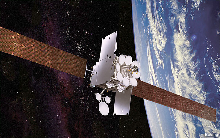
Figure 1: Inmarsat-5 F2 satellite

Notably, that solar panels may experience heavy vibrations due to the environmental effects [5]. Hence, different mode shapes of the vibrating system should be taken into account.

Various techniques are accomplished to find the solution for vibration analysis of shells and plates under specific forms of loading and boundary conditions, series-type method [6] and integral equations method [7, 8], to name a few. Leissa also presented an inclusive and accurate analytical approach for the solution of the free vibration in rectangular plates [9, 10, 7]. Moreover, finite element (FE) and finite strip method (FSM) [11, 12, 13], Rayleigh-Ritz method [14], Galerkin method [15], domain decomposition method [16, 17], energy balance method (EBM) [18], differential quadrature (DQ) [19], and generalized differential quadrature (GDQ) methods [20, 21] are among different techniques proposed within literature.

The DQ and GDQ methods have been developed by Bellman and Casti [22] and Shu and Richards [23]. The efficiency in computing the weighting coefficients is the principal advantage of GDQ due to its simplicity in the choice of grid points. For the vibration analysis of plates and shells, various studies concerning the validity of DQ/GDQ methods exist in the scientific literature. Most of these studies have investigated typical cases including a combination of standard boundary conditions and uniformly distributed loads. For rectangular plates with different shapes of holes, an independent coordinate coupling method is employed for vibration analysis [24]. Additionally, local effects such as the vibration of rectangular plates with concentrated mass–springs [25], distinct elastic edge restraints [26], and thermal nonlinear vibration of the orthotropic DLGS [27] are investigated within the literature.

This study investigates combined torsional and transverse vibration analysis of a solar panel including a completely free rectangular plate locally supported by an elastic beam. By applying the GDQ method, the domain of the solution together with governing PDEs for the beam and plate are discretized. Based on governing equations along with boundary and continuity conditions, the final eigenvalue problem is developed. The solution to the final equations leads to eigenvalues and eigenvectors which are respectively natural frequencies and mode shapes of the system. To assess the reliability of the proposed method, results for various simplified case studies, in Section 5, are evaluated with available analytical and numerical solutions within the literature. For the complicated cases, results are also validated by commercial FE code, due to lack of information in the literature. Finally, frequency predictions and mode shapes of the general case show an acceptable correlation with finite element results. It is expecting that the results of this paper can be utilized as a benchmark in future studies dealing with the combined transverse and torsional vibration analysis of suspended plates and panels.

2 Modeling

The system comprises a rectangular isotropic thin elastic plate with dimensions of $a\times b$ and thickness of $h$. The plate is locally attached to a clamped beam with length $l$ and the cross-section of $t\times d$, as shown in Fig. 2. Considering the possibility of resonance in the vibration of the plates, one should pay attention to the material properties and geometry of the system. The plate and the beam are elastic with $E_{1}$, $E_{2}$ as modulus of elasticity, and ${\nu}_{1}$, ${\nu}_{2}$ as Poisson’s ratio, respectively.

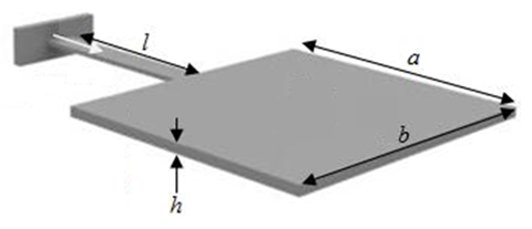
Figure 2: Schematic model

Also, $G_{1}$ and $I_{1}$ are shear modulus and polar moment of inertia of the beam, respectively. Due to external excitation, the system may start to vibrate in the form of transverse and/or torsional vibration. Assuming $W(x,y,t)$ as the deflection of the plate, and $U(x^{\prime},t)$ and $\theta(x^{\prime},t)$ as deflection and rotation of the beam, the governing equations of the system can be obtained as [7]:

$$E_{1}I_{1}\frac{\partial^{4}U(x^{\prime},t)}{\partial{x^{\prime}}^{4}}+{\rho}_{1}A_{1}\frac{\partial^{2}U(x^{\prime},t)}{\partial t^{2}}=0$$ (1a)

$$G_{1}J_{1}\frac{\partial^{2}\theta(x^{\prime},t)}{\partial{x^{\prime}}^{2}}=\rho_{1}I_{1}\frac{\partial^{2}\theta(x^{\prime},t)}{\partial t^{2}}$$ (1b)

$$D\frac{\partial^{4}W(x,y,t)}{\partial x^{4}}+2D\frac{\partial^{4}W(x,y,t)}{\partial x^{2}\partial y^{2}}+D\frac{\partial^{4}W(x,y,t)}{\partial y^{4}}+{\rho}_{2}h\frac{\partial^{2}W(x,y,t)}{\partial t^{2}}=0$$ (1c)

in which $x^{\prime}=x+l$ and $A_{2}=t\times d$ is the cross-sectional area of the beam. $\rho_{1}$ and $\rho_{2}$ are respectively mass densities of the beam and the plate. Also, $D$ is the flexural rigidity of the plate, which can be determined as

$$D=\frac{E_{1}h^{3}}{12(1-{\upsilon}^{2}_{2})}$$ (2)

Assuming $u(x^{\prime},t)=U(x^{\prime})e^{i\omega^{z}_{b}t}$, $\theta(x^{\prime},t)=\Theta(x^{\prime})e^{i\omega^{\phi}_{b}t}$, and $w(x\mathrm{,y,}t)=W(x,y)e^{i\omega_{p}t}$, one may rewrite Eq. 1 as follows

$$\frac{\partial^{4}U}{\partial{X^{\prime}}^{4}}={{\overline{\omega}}^{z}_{b}}^{2}U$$ (3a)

$$\frac{\partial^{2}\Theta}{\partial X^{2}}+{{\overline{\omega}}^{\phi}_{b}}^{2}\Theta=0$$ (3b)

$$\frac{\partial^{4}W}{\partial X^{4}}+2\beta^{2}\frac{\partial^{4}W}{\partial X^{2}\partial Y^{2}}+\beta^{4}\frac{\partial^{4}W}{\partial Y^{4}}={{\overline{\omega}}_{p}}^{2}W$$ (3c)

where $\omega^{z}_{b}$ and ${\omega}^{\phi}_{b}$ are natural frequencies for transverse and torsional vibration of the beam, respectively, and $\omega_{b}$ is natural frequency for vibration of plate.

Also, other parameters are defined as

$${\overline{\omega}}_{b}^{z^{2}}=\frac{\rho_{1}AL^{4}}{E_{1}I}\omega_{b}^{z^{2}}$$

$${\overline{\omega}}_{b}^{\phi^{2}}=\frac{\rho IL^{2}}{GJ}\omega_{b}^{\phi^{2}}$$

$${{\overline{\omega}}_{p}}^{2}=\frac{\rho_{2}ha^{4}}{D}\omega^{2}_{p}$$

$$X^{\prime}=\frac{x^{\prime}}{L\beta}=\frac{a}{b}$$

$$X=\frac{x}{a},\quad Y=\frac{y}{b}$$

Note that the length of the plate is defined as $a$, while $b$ is the plate width. Generally, for a thin plate, shear forces and moments are

$$\begin{cases}V_{x}=-D\left(\frac{\partial^{3}W}{\partial x^{3}}+(2-v_{2})\frac{\partial^{3}W}{\partial x\partial y^{2}}\right)\\ V_{y}=-D\left(\frac{\partial^{3}W}{\partial y^{3}}+(2-v_{2})\frac{\partial^{3}W}{\partial x^{2}\partial y}\right)\end{cases}$$ (4a)

$$\left[\begin{array}[]{c}M_{x}\\ M_{y}\\ M_{z}\end{array}\right]=-D\left[\begin{array}[]{ccc}1&v_{2}&0\\ v_{2}&1&0\\ 0&0&1-v_{2}\end{array}\right]\left[\begin{array}[]{c}\frac{\partial^{2}W}{\partial x^{2}}\\ \frac{\partial^{2}W}{\partial y^{2}}\\ \frac{\partial^{2}W}{\partial x\partial y}\end{array}\right]$$ (4k)

Implementation of boundary conditions, which refers to the free edges of the plate and clamped side of the beam, as well as continuity of displacements, shear forces, and bending moments at the attached points should be considered. Therefore, boundary equations for the beam section can be written as

$$u(0,t)=0$$ (5a)

$$\frac{\partial u(0,t)}{\partial x^{\prime}}=0$$ (5b)

$$\theta(0,t)=0$$ (5c)

Also, boundary conditions at free edges of the plate are

$$\frac{\partial^{2}w(a,y,t)}{\partial x^{2}}+\nu_{2}\beta^{2}\frac{\partial^{2}w(a,y,t)}{\partial y^{2}}=0$$ (6a)

$$\frac{\partial^{2}w(0,y,t)}{\partial x^{2}}+\nu_{2}\beta^{2}\frac{\partial^{2}w(0,y,t)}{\partial y^{2}}=0\quad{\rm for}\ |y|\geq\frac{d}{2}$$ (6b)

$$\beta^{2}\frac{\partial^{2}w(x,0,t)}{\partial y^{2}}+\nu_{2}\frac{\partial^{2}w(x,0,t)}{\partial x^{2}}=0$$ (6c)

$$\beta^{2}\frac{\partial^{2}w(x,b,t)}{\partial y^{2}}+\nu_{2}\frac{\partial^{2}w(x,b,t)}{\partial x^{2}}=0$$ (6d)

and

$$\frac{\partial^{3}w(a,y,t)}{\partial x^{2}}+(2-\nu_{2})\beta^{2}\frac{\partial^{2}w(a,y,t)}{\partial x\partial y^{2}}=0$$ (7a)

$$\frac{\partial^{2}w(0,y,t)}{\partial x^{2}}+(2-\nu_{2})\beta^{2}\frac{\partial^{2}w(0,y,t)}{\partial x\partial y^{2}}=0\quad{\rm for}\ |y|\geq\frac{d}{2}$$ (7b)

$$\beta^{2}\frac{\partial^{3}w(x,0,t)}{\partial y^{2}}+(2-\nu_{2})\frac{\partial^{3}w(x,0,t)}{\partial x^{2}\partial y}=0$$ (7c)

$$\beta^{2}\frac{\partial^{3}w(x,b,t)}{\partial y^{3}}+(2-\nu_{2})\frac{\partial^{3}w(x,b,t)}{\partial x^{2}\partial y}=0$$ (7d)

Continuity conditions at the attached points can be written as

$$u(l,t)=w(0,y,t)$$ (8a)

$$\frac{\partial u(l,t)}{\partial x^{\prime}}=\frac{\partial w(0,y,t)}{\partial x}$$ (8b)

$$E_{1}I_{1}\frac{\partial^{2}u(l,t)}{\partial{x^{\prime}}^{2}}=D\left(\frac{\partial^{2}w(0,y,t)}{\partial x^{2}}+\nu_{2}\frac{\partial^{2}w(0,y,t)}{\partial y^{2}}\right)$$ (8c)

$$E_{1}I_{1}\frac{\partial^{3}u(l,t)}{\partial{x^{\prime}}^{2}}=D\left(\frac{\partial^{2}w(0,y,t)}{\partial x^{2}}+(2-\nu_{2})\frac{\partial^{2}w(0,y,t)}{\partial x\partial y^{2}}\right)$$ (8d)

in which the domain of $y$ in Eqs. 8 is $|y|\geq\frac{d}{2}$.

3 GDQ Implementation

To commence the procedure of GDQ method, the domain of the solution should be first discretized into several grid points. Zeros of the Chebyshev polynomials is one of the best choices to discretize the domain, see [28]. As a result, the plate is discretized into $N\times M$ grid points in $x$ and $y$ directions, respectively, while the beam may be divided into three or five rows of $S$ grid points through $x$ direction, as shown in Fig. 3. Afterward, governing partial differential equations are expanded over these grid points. By assuming three or five rows of grid points in the width of the beam, continuity conditions can be satisfied.

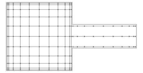
Figure 3: Discretization of the system into grid points

According to the GDQ method, a general form of the approximation for the calculation of higher-order derivatives is

$$u^{m}_{x}(x_{i},t)=\sum^{b}_{j=1}\tau^{(m)}_{ij}u(x_{j},t)\qquad{\rm for}\quad i=1,\cdots,S$$ (9)

where $u^{m}_{x}(x_{i},t)$ is the $m^{\rm th}$ derivative of beam deflection at point $(x_{i},b)$ is the number of grid points and $\tau^{(m)}_{ij}$ is the weighting coefficients for the $m^{\rm th}$ derivative calculation. The grid points on the beam and plate based on zeros of the Chebyshev polynomials can be determined as:

$$x^{\prime}_{k} =\frac{L}{2}\left[1-{{\rm cos}\left(\frac{k-1}{S-1}\pi\right)}\right]$$ (10a)

$$x_{i} =\frac{a}{2}\left[1-{{\rm cos}\left(\frac{i-1}{N-1}\pi\right)\ }\right]$$ (10b)

$$y_{j} =\frac{b}{2}\left[1-{{\rm cos}\left(\frac{j-1}{M-1}\pi\right)\ }\right]$$ (10c)

In discretization, Eq. (11) gives the weighting coefficients for higher order derivatives

$$\zeta^{(m)}_{rk}=m\left(\eta^{(m-1)}_{rr}\eta^{(1)}_{rk}-\frac{\eta^{(m-1)}_{rk}}{{x^{\prime}}_{r}-{x^{\prime}}_{k}}\right)\quad\qquad{\rm for}\quad r\neq k\quad r,k=1,\cdots,S$$ (11a)

$$c^{(m)}_{pi}=m\left(c^{(m-1)}_{pp}c^{(1)}_{pi}-\frac{c^{(m-1)}_{pi}}{x_{p}-x_{i}}\right)\quad\qquad{\rm for}\quad r\neq k\quad r,k=1,\cdots,S$$ (11b)

$${\overline{c}}^{(m)}_{lj}=m\left({\overline{c}}^{(m-1)}_{ll}{\overline{c}}^{(1)}_{lj}-\frac{{\overline{c}}^{(m-1)}_{lj}}{y_{l}-y_{j}}\right)\quad\qquad{\rm for}\quad r\neq k\quad r,k=1,\cdots,S$$ (11c)

The $\zeta^{(m)}_{rk}$, $c^{(m)}_{pi}$, and ${\overline{c}}^{(m)}_{lj}$ can be respectively derived based on the $(m-1)^{\rm th}$ order coefficients $\zeta^{(m-1)}_{rk}$, $c^{(m-1)}_{pi}$, and ${\overline{c}}^{(m-1)}_{lj}$. The $\zeta^{(m)}_{rk}$, $c^{(m)}_{pi}$, and ${\overline{c}}^{(m)}_{lj}$ can be obtained from:

$$\zeta^{(m)}_{rr} =\sum^{S}_{\begin{array}[]{c}k=1\\ k\neq r\end{array}}\zeta^{(m)}_{rk}\qquad{\rm for\ }\ r=1,\cdots,S$$ (12c)

$$c^{(m)}_{pp} =\sum^{N}_{\begin{array}[]{c}l=1\\ l\neq p\end{array}}c^{(m)}_{pl}\qquad{\rm for\ }\ p=1,\cdots,N$$ (12f)

$${\overline{c}}^{(m)}_{ll} =\sum^{M}_{\begin{array}[]{c}j=1\\ j\neq l\end{array}}{\overline{c}}^{(m)}_{ij}\qquad{\rm for\ }\ l=1,\cdots,M$$ (12i)

Based on the recursive formulas 11 and 12, ${\eta}^{(1)}_{rk}$, $c^{(1)}_{pi}$ and ${\overline{c}}^{(1)}_{lj}$ can be calculated as follow:

$$\eta^{(1)}_{rk}=\frac{\mathrm{P}({x^{\prime}}_{r})}{({x^{\prime}}_{r}-{x^{\prime}}_{k})\mathrm{P}({x^{\prime}}_{k})}\qquad{\rm for\ }\ r\neq k$$ (13a)

$$c^{(1)}_{pi}=\frac{Q(x_{p})}{(x_{p}-x_{i})Q(x_{i})}\qquad{\rm for\ }\ p\neq i$$ (13b)

$${\overline{c}}^{(1)}_{lj}=\frac{H(y_{l})}{(y_{l}-y_{j})H(y_{j})}\qquad{\rm for\ }\ l\neq j$$ (13c)

where

$$P(x^{\prime}_{r})=\prod^{S}_{\begin{array}[]{c}k=1\\ k\neq r\end{array}}{\left({x^{\prime}}_{r}-{x^{\prime}}_{k}\right)},\qquad Q(x_{p})=\prod^{N}_{\begin{array}[]{c}i=1\\ i\neq p\end{array}}{\left(x_{p}-x_{i}\right)},\qquad H(x_{l})=\prod^{M}_{\begin{array}[]{c}j=1\\ j\neq l\end{array}}{\left(x_{l}-x_{j}\right)}$$ (20)

Also, one may obtained $\eta^{(1)}_{kk}$, $c^{(1)}_{ii}$ and ${\overline{c}}^{(1)}_{jj}$ using:

$${\eta}^{(1)}_{kk} =-\sum^{S}_{\begin{array}[]{c}k=1\\ k\neq r\end{array}}{{\eta}^{(1)}_{rk}}\qquad{\rm for\ }\ r=1,2,\cdots,N$$ (21c)

$$c^{(1)}_{ii} =-\sum^{N}_{\begin{array}[]{c}i=1\\ i\neq p\end{array}}{c^{(1)}_{pi}}\qquad{\rm for\ }\ p=1,2,\cdots,N$$ (21f)

$${\overline{c}}^{(1)}_{jj} =-\sum^{M}_{\begin{array}[]{c}j=1\\ j\neq l\end{array}}{{\overline{c}}^{(1)}_{lj}}\qquad{\rm for\ }\ l=1,2,\cdots,N$$ (21i)

According to the definition of the derivative terms and applying the GDQ approximation, Eq. (3) can be rewritten as

$$\sum^{S}_{k=1}{\zeta^{(4)}_{rk}U_{k}}={\overline{\omega}}^{2}U_{r}$$ (22a)

$$\sum^{S}_{k=1}{\zeta^{(2)}_{rk}\Theta_{k}}=-{{\overline{\omega}}^{\phi}_{b}}^{2}\Theta_{r}\quad{\rm for}r=3,\cdots,S-2$$ (22b)

$$\sum^{N}_{k=1}{c^{(4)}_{ik}W_{kj}}+2\beta^{2}\sum^{M}_{m=1}{{\overline{c}}^{(2)}_{jm}}\sum^{N}_{k=1}{c^{(2)}_{ik}W_{km}}+\beta^{4}\sum^{M}_{m=1}{{\overline{c}}^{(4)}_{jm}W_{im}}={{\overline{\omega}}_{p}}^{2}W_{ij}$$ (22c)

for $i=3,\cdots,N-2$ and $j=3,\cdots,M-2$. It is worth mentioning that the aforementioned equations should be considered for all grid points except boundary and adjacent nodes, see [29]. Boundary conditions for the beam section at the fixed end, which have been written in Eq. (5), can be respectively discretized as $U_{1}=0$, $\sum^{S}_{k=1}\zeta^{(1)}_{1k}U_{k}=0$, and $\Theta_{1}=0$.

In addition to that, the discretized forms of the boundary conditions of zero normal moment at free edges in Eqs. (6) and (7) are

$$\sum^{N}_{k=1}{c^{(2)}_{Nk}W_{kj}}+\nu_{2}\beta^{2}\sum^{M}_{m=1}{{\overline{c}}^{(2)}_{jm}W_{Nm}}=0$$ (23a)

$$\sum^{N}_{k=1}{c^{(2)}_{1k}W_{kj}}+\nu_{2}\beta^{2}\sum^{M}_{m=1}{{\overline{c}}^{(2)}_{jm}W_{1m}}=0\qquad{\rm for\ }j=3,4,\cdots,M-3,M-2,{\rm and}$$

$$\beta^{2}\sum^{M}_{m=1}{{\overline{c}}^{(2)}_{1m}W_{im}}+\nu_{2}\sum^{N}_{k=1}{c^{(2)}_{ik}W_{k1}}=0$$ (23b)

$$\beta^{2}\sum^{M}_{m=1}{{\overline{c}}^{(2)}_{Mm}W_{im}}+\nu_{2}\sum^{N}_{k=1}{c^{(2)}_{ik}W_{kM}}=0\qquad{\rm for\ }i=1,2,\cdots,N$$

Also, we have

$$\sum^{N}_{k=1}{c^{(3)}_{Nk}W_{kj}}+(2-\nu_{2}){\beta}^{2}\sum^{N}_{k=1}{c^{(1)}_{Nk}}\sum^{M}_{m=1}{{\overline{c}}^{(2)}_{jl}W_{km}}=0$$ (24a)

$$\sum^{N}_{k=1}{c^{(3)}_{1k}W_{kj}}+(2-\nu_{2})\beta^{2}\sum^{N}_{k=1}{c^{(1)}_{1k}}\sum^{M}_{m=1}{{\overline{c}}^{(2)}_{jl}W_{km}}=0\qquad{\rm for\ }j=3,4,\cdots,M-3,M-2,{\rm and}$$

$$\beta^{2}\sum^{M}_{m=1}{{\overline{c}}^{(3)}_{1m}W_{im}}+(2-\nu_{2})\sum^{N}_{k=1}{c^{(2)}_{1m}}\sum^{M}_{m=1}{{\overline{c}}^{(1)}_{ik}W_{km}}=0$$ (24b)

$$\beta^{2}\sum^{M}_{m=1}{{\overline{c}}^{(3)}_{Mm}W_{im}}+(2-\nu_{2})\sum^{N}_{k=1}c^{(2)}_{Mm}\sum^{M}_{m=1}{{\overline{c}}^{(1)}_{ik}W_{km}}=0\qquad{\rm for\ }i=1,2,\cdots,N$$

Moreover, the continuity condition for the local part (Eq. (8)) can be written as follows

$$U_{S}=W_{1j}$$ (25a)

$$\sum^{S}_{r=1}{\zeta^{(1)}_{Sr}U_{i}}=\sum^{N}_{k=1}{c^{(1)}_{1k}W_{kj}}$$ (25b)

$$E_{1}I_{1}\sum^{S}_{r=1}{\zeta^{(2)}_{Sr}U_{r}}=-D\left(\sum^{N}_{k=1}{c^{(2)}_{1k}W_{\mathrm{kj}}}+\nu_{2}\sum^{M}_{m=1}{{\overline{c}}^{(2)}_{jm}W_{1m}}\right)$$ (25c)

$$E_{1}I_{1}\sum^{S}_{r=1}{\zeta^{(3)}_{Sr}U_{r}}=-D\left(\sum^{N}_{k=1}{c^{(2)}_{1k}W_{kj}}+(2-\nu_{2})\sum^{N}_{k=1}{c^{(1)}_{1k}}\sum^{M}_{m=1}{{\overline{c}}^{(2)}_{jm}W_{km}}\right)$$ (25d)

in which the domain of $k$ in Eqs. 25 is $(\frac{b-d}{2})(\frac{N-1}{b})+1\leq j\leq(\frac{b+d}{2})(\frac{N-1}{b})+1$.

4 Solution procedure

Considering governing Eqs. (22), boundary conditions (23) and (24) and continuity conditions (25), one can write these systems of equations in form of two sets of algebraic equations as following:

$$\left[A_{IB}\right]\left\{W_{B}\right\}+\left[A_{II}\right]\left\{W_{I}\right\}={\Omega}^{2}\left\{W_{I}\right\}$$ (26a)

$$\left[A_{BB}\right]\left\{W_{B}\right\}+\left[A_{BI}\right]\left\{W_{I}\right\}=0$$ (26b)

where $\{W_{B}\}$ and $\{W_{I}\}$ are nodes deflection inside the domain and on boundaries, respectively. Furthermore, dimensions of $[A_{II}]_{P\times P}$, $[A_{BB}]_{Q\times Q}$, $[A_{IB}]_{P\times Q}$ and $[A_{BI}]_{Q\times P}$ are defined such that $P=(S-4)+(M-4)\times(N-4)$ and $Q=(4M+4N-12)$.

Substitution of Eq. (26a) in (26b) gives the final system of eigenvalue equation as:

$$\left\{\left[A_{II}\right]-\left[A_{IB}\right]{[A_{BB}]}^{-1}\left[A_{BI}\right]\right\}\{W_{I}\}={\omega}^{2}\{W_{I}\}$$ (27)

The standard form of eigenvalue equation can be obtained by restating Eq. (27) as

$$\left[\left\{\left[A_{II}\right]-\left[A_{IB}\right]{[A_{BB}]}^{-1}\left[A_{BI}\right]\right\}-I\right]\{W_{I}\}={\omega}^{2}\left\{W_{I}t\right\}$$ (28)

where $\{I\}$ is the identity matrix. After implementing the values in stiffness matrix in Eq. (21), by solving this standard eigenvalue equation, natural frequencies of the system together with related mode shapes could be determined.

5 Results and discussions

Free torsional and transverse vibration analysis of a system comprises a free plate locally supported by an elastic beam is presented. At first, three types of equations, i.e. governing equations, equations of boundary conditions and equations of continuity conditions are developed. To solve these equations, GDQ method is applied to the domain of the solution. Accordingly, both domains of the solution and governing equations, together with boundary/continuity equations are discretized. Thereafter, all equations are rewritten in the form of two sets of equations giving the final system of eigenvalue equation. The system is eventually simplified into several widely-known cases of vibration analysis, e.g. completely free (FFFF) plate, cantilever (CFFF) plate, clamped-free beam and beam with concentrated mass, to determine the accuracy of the proposed solution, the system is simplified into several. Also, the general model has been investigated in the final case in which the accuracy of the results is evaluated. Table 1 shows the properties of the plate and beam.

Table 1: Material and geometry properties

Properties	Values
$a$	$1\ m$
$b$	$1\ m$
$L$	$1\ m$
$d$	$0.1\ m$
$t$	$0.5\ cm$
$\nu_{1},\nu_{2}$	$3\ cm$
$\rho_{1},\rho_{2}$	$2330\ kg/m^{3}$
$E_{1},E_{2}$	$200\ GPa$

Case study 1 As the first case study, material properties and geometry parameters for the plate are assumed to be the same as those of the beam which simplifies the model to a simple cantilever beam. Hence, identical width, thickness and material properties should be considered, i.e. $t=h,d=2b,E_{1}=E_{2},\rho_{1}=\rho_{2}$. Moreover, the Poisson ratio of the plate section should be neglected to eliminate the deformation of the plate in the $y$ direction. Taking into account the aforementioned properties, the model is simplified to a homogeneous clamped–free beam with length$\ L^{*}=L+a$. Due to the attachment of the plate to the end of the beam, vibration of the plate may cause torsional vibration over the beam. Therefore, 2D discretization is applied through the domain of the beam. It is worth mentioning that analytical solutions can be found for natural frequencies of both transverse and torsional vibrations of clamped-free beams using modal analysis as [6]:

$${\rm cos}\beta L^{*}\times\mathrm{cosh}\beta L^{*}+1=0$$ (29a)

$$\mathrm{cos}\frac{\omega^{\theta}_{j}L^{*}}{c}=0$$ (29b)

in which

$$\beta^{4}=\frac{\rho A({\omega^{z}_{i})}^{2}}{EI},\qquad c=\sqrt{\frac{G}{\rho}},\qquad\omega_{j}^{\theta}=\frac{\alpha_{j}c}{l}$$

Note that $\omega^{z}_{i}$ and $\omega^{\theta}_{j}$ are respectively the $i^{\rm th}$ natural frequency of transverse vibration and $j^{\rm th}$ natural frequency of torsional vibration of the beam.

Tables 2 and 3 respectively demonstrate the first eight natural frequencies of the system for both transverse and torsional vibration, computed by both GDQ and frequency Eqs. (29).

Table 2: First eight natural frequencies of transverse vibration of clamped-free beam

Method/Grid Size	$\Omega_{1}$	$\Omega_{2}$	$\Omega_{3}$	$\Omega_{4}$	$\Omega_{5}$	$\Omega_{6}$	$\Omega_{7}$	$\Omega_{8}$
Exact Method (Eq. 22.a)	1.875	4.694	7.855	10.996	14.137	17.279	20.420	23.562
$5\times 9$	1.845	4.569	7.736	10.825	13.984	17.259	20.390	23.493
$5\times 11$	1.863	4.679	7.839	10.971	14.120	17.264	20.402	23.540
$5\times 15$	1.875	4.695	7.843	10.982	14.129	17.268	20.407	23.549
Error (%)	0.0320	0.0128	0.1515	0.1255	0.0559	0.0602	0.0686	0.0531

Another simple case can be considered by assuming a plate with large density and small sizes which reduces the model to a simple cantilever beam with concentrated end mass. To achieve this, the plate is assumed to be made of Lead with density equals to $\rho_{1}=11.34\ gr/cm^{3}$ and geometry properties as $a=b=h=0.1m$. Again, the frequency equation for transverse and torsional vibration of this simple case can be found analytically as [6]:

$$1+\frac{1}{{\rm cos}(\beta l)\ {\rm cosh}(\beta l)}-R_{z}\ \beta l\left({{\rm tan}(\beta l)-{\rm tanh}(\beta l)}\right)=0$$ (31a)

$$\beta^{4}=\frac{\rho A({\omega^{z}_{i})}^{2}}{EI}$$ (31b)

$$\alpha_{j}\ {\rm tan}(\alpha_{j})=R_{\theta}$$ (31c)

$$\omega^{\theta}_{j}=\frac{\alpha_{j}c}{l}$$ (31d)

Table 3: First eight natural frequencies of torsional vibration of clamped-free beam

Method/Grid Size	$\Omega_{1}$	$\Omega_{2}$	$\Omega_{3}$	$\Omega_{4}$	$\Omega_{5}$	$\Omega_{6}$	$\Omega_{7}$	$\Omega_{8}$
Exact Method (Eq. 22.b)	1.571	4.712	7.854	10.996	14.137	17.279	20.420	23.562
$5\times 9$	1.571	4.715	7.875	11.096	14.178	17.2910	20.462	23.583
$5\times 11$	1.571	4.714	7.864	10.796	14.158	17.289	20.442	23.573
$5\times 15$	1.571	4.710	7.852	10.988	14.128	17.281	20.418	23.573
Error (%)	0.013	0.045	0.024	0.071	0.067	0.014	0.011	0.045

where $R_{z}=\frac{M}{\rho Al}$ is the ratio of the attached mass $M$ to the mass of the beam $\rho Al$. Also, $R_{\theta}$ is equal to $\frac{\rho jl}{I_{d}}$ in which $I_{d}$ is the moment of inertia of the plate and $\rho,j$ and $l$ are properties of the beam. Based on the proposed geometry and material properties, one may obtain $R_{z}=9.734$ and $R_{\theta}=0.051$. Similarly, Tables 4 and 5 contain first eight natural frequencies of the beam with concentrated mass, obtained by GDQ and Eqs. 31. Results show reasonably accurate predictions for both cases.

Table 4: First eight natural frequencies of clamped-free beam with concentrated mass $R_{z}=9.734$; transverse vibration

Method / Grid Size	Transverse Frequencies: $R_{z}=9.734$
	$\Omega_{1}$	$\Omega_{2}$	$\Omega_{3}$	$\Omega_{4}$	$\Omega_{5}$	$\Omega_{6}$	$\Omega_{7}$	$\Omega_{8}$
Exact Method (Eq. 23.a)	0.741	1.571	3.939	4.712	7.076	7.854	10.215	10.996
$5\times 9$	0.763	1.597	3.948	4.733	7.284	7.963	10.321	10.962
$5\times 11$	0.726	1.586	3.929	4.724	7.176	7.859	10.319	10.977
$5\times 15$	0.740	1.571	3.938	4.709	7.069	7.853	10.208	10.989
Error (%)	0.0675	0.0255	0.0102	0.0785	0.0862	0.0115	0.0705	0.0591

Table 5: First eight natural frequencies of clamped-free beam with concentrated mass $R_{\theta}=0.051$; torsional vibration

Method / Grid Size	Torsional Frequencies; $R_{\theta}=0.051$
	$\Omega_{1}$	$\Omega_{2}$	$\Omega_{3}$	$\Omega_{4}$	$\Omega_{5}$	$\Omega_{6}$	$\Omega_{7}$	$\Omega_{8}$
Exact Method (Eq. 23.b)	1.571	3.158	4.712	6.291	7.854	9.430	10.996	12.571
$5\times 9$	1.573	3.160	4.715	6.294	7.869	9.459	11.054	12.549
$5\times 11$	1.572	3.159	4.714	6.293	7.867	9.449	11.005	12.560
$5\times 15$	1.570	3.157	4.710	6.290	7.849	9.421	10.985	12.562
Error (%)	0.0382	0.0443	0.0552	0.0286	0.0701	0.1007	0.0946	0.0684

Case study 2 As another simple case for evaluation of the model and solution procedure, one may ignore the effects of the beam by assuming zero geometry and material parameters which reduces the system to a completely free plate. As a result, the beam exerts no force and moment on the plate. Table 6 includes the results of first five natural frequencies obtained by GDQ method. Also, table 6 shows the results of direct GDQ method obtained by Shu and Du [29], analytical results presented by Leissa [9, 10] and also results obtained using commercial FE code ANSYS. Predictions show good correlations with other methods. It is worth mentioning that by reselecting grid points by modified formulation provided in [29], the accuracy of the results is significantly improved.

Table 6: First five natural frequencies of FFFF plate

Method / Grid Size	$\Omega_{1}$	$\Omega_{2}$	$\Omega_{3}$	$\Omega_{4}$	$\Omega_{5}$	$\Omega_{6}$
Leissa [9]	13.489	19.789	24.432	35.024	35.024	61.526
Leissa & Narita [10]	13.468	19.596	24.271	34.801	34.801	61.111
Shu and Du (15*15) [29]	10.303	19.596	22.146	30.026	30.803	-
Shu and Du(12*12) [29]	13.454	19.597	24.271	34.815	34.817	-
FEM	13.461	19.665	24.289	34.912	34.825
GDQ
$9\times 9$	10.934	19.365	21.935	29.432	29.536	-
$11\times 11$	10.639	19.685	22.854	31.342	30.762	-
$15\times 15$	10.303	19.596	22.146	30.026	30.803	-
Error (%)	23.619	0.975	9.356	14.270	12.051
Modified GDQ
$9\times 9$	14.065	19.968	24.696	34.938	34.645	-
$11\times 11$	13.164	19.492	24.434	34.884	34.783	-
$15\times 15$	13.475	19.598	24.268	34.832	34.828	-
Error (%)	0.103	0.965	0.671	0.548	0.559

Case study 3 As the final test case to evaluate the performance of the presented method, the beam is considered to be rigid with identical widths for both the beam and plate. This will reduce the system to a cantilever plate. To this end, the Young and shear modulus of elasticity of the beam should tend to infinity. Table 7 includes the GDQ predictions for the first five natural frequencies of the plate. Also, the result of direct GDQ and the analytical method by Leissa [9, 10] are presented in Table 7. To prove the validity of the presented method, results of FE code (ANSYS) are also included in the table. To develop the accuracy of the method, the same procedure as the previous case study may be applied. The new results are presented in Table 7 as well.

Table 7: First five natural frequencies of CFFF plate

Method / Grid Size	$\Omega_{1}$	$\Omega_{2}$	$\Omega_{3}$	$\Omega_{4}$	$\Omega_{5}$	$\Omega_{6}$
Leissa [4]	3.492	8.525	21.429	27.331	31.111	54.443
Shu and Du (15*15) [29]	3.898	9.459	20.206	26.150	26.500	-
Shu and Du (12*12) [29]	3.485	8.604	21.586	27.230	31.358	-
FEM	3.481	8.502	21.456	27.401	30.021
GDQ
$9\times 9$	3.486	8.616	19.894	25.965	27.925	-
$11\times 11$	3.768	8.914	20.065	26.425	29.682	-
$15\times 15$	3.898	9.459	20.206	26.150	26.500	-
Error (%)	11.626	10.956	5.707	4.321	14.821
Modified GDQ
$9\times 9$	3.467	8.725	21.104	26.935	31.825	-
$11\times 11$	3.482	8.625	21.238	27.189	31.539	-
$15\times 15$	3.495	8.564	21.462	27.312	31.261	-
Error (%)	0.085	0.457	0.154	0.069	0.482

Case study 4: The final case is the complicated system consists of a regionally suspended plate connected to the elastic beam. The standard form of eigenvalue equations for the combined transverse/torsional vibration of the system is solved and consequently eigenvalues and eigenvectors are derived. To validate the calculation procedure, finite element code ANSYS was also used to analyze the system. Figures 4 to 8 depicts five different mode shapes of the system together with associated frequencies, which are predicted by the presented GDQ technique. As shown in these figures, the system can vibrate based on various mode shapes of the beam and the plate and also their combination. For instance, Figs. 4 and 5 depict mode shapes of the system once the first modes of transverse and torsional vibrations of the beam are excited, respectively. Besides, Figs. 6 to 8 show mode shapes of the system as the modes of beam and plate are simultaneously excited. Included in these figures are also results of FE analysis for both frequencies and mode shapes of the system, which indicates reasonable accuracy for the proposed approach. The range of errors in predictions is about $4.4\%$ to $7.8\%$, in which minimum and maximum errors belong to predicted frequencies of $2.675$ Hz and $147.494$ Hz, respectively.

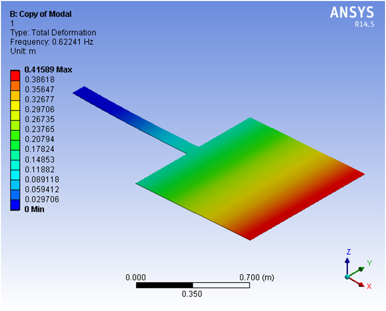
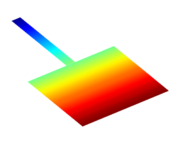
Figure 4: First mode shape of transverse vibration of the beam

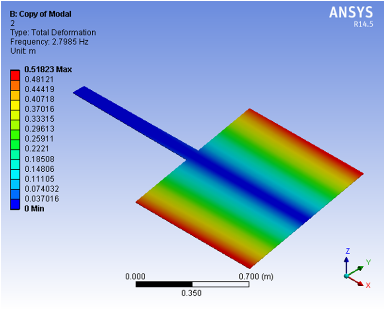
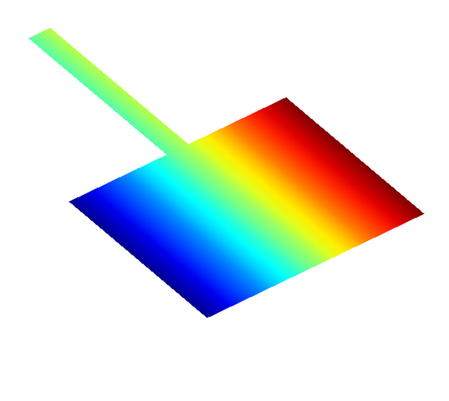
Figure 5: First mode shape of torsional vibration of the beam

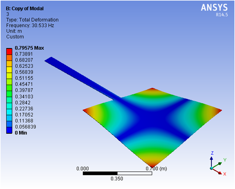
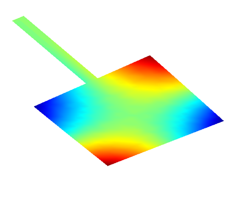
Figure 6: First mode shape of torsional vibration of the beam together with first mode shape of the plate

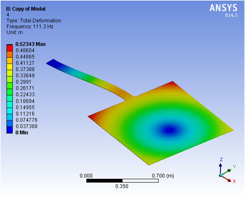
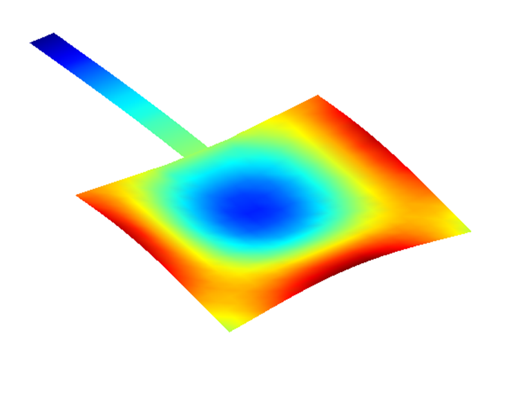
Figure 7: First mode shape of transverse vibration of the beam together with second mode shape of the plate

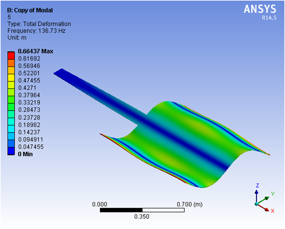
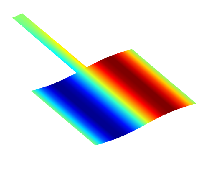
Figure 8: First mode shape of torsional vibration of the beam together with forth mode shape of the plate

6 Conclusion

This study is dedicated to investigate combined torsional and transverse free vibration analysis of thin plates locally supported by an elastic beam. In particular, the performance of the GDQ method to offer solutions for practical problems with local effects is examined. Using Euler-Bernoulli assumption and classical plate theory, two coupled governing PDEs together with continuity/boundary conditions are developed based on the GDQ method. All equations are then restated as two sets of algebraic equations. The solution to the final equations leads to eigenvalues and eigenvectors that respectively indicate the system’s natural frequencies and mode shapes. To assess the reliability of the proposed method, results for different well-known cases are compared by available analytical and numerical methods. This includes examples of several well-known cases of classical vibration such as cantilever beam, beam with concentrated mass, FFFF and CFFF plate. Results revealed that predictions in these case studies are in close correlation with analytical/numerical results while the accuracy can also be remarkably increased by reselecting the grid points.

Finally, predictions for the complicated system are validated by commercial FE code ANSYS, due to lack of information within the literature. Comparisons for different frequencies and mode shapes with FE results are encouraging particularly for systems with local boundary and continuity conditions. Considering the performance of the presented modeling and solution technique, it is expected to be used as a benchmark for vibration analysis of suspended plates/shells and panels in future theoretical and experimental studies.

References

- [1] M Amereh, MM Aghdam, and M Golkaram. Design and modeling of a novel translational and angular micro-electromechanical accelerometer. Aerospace Science and Technology, 50:15–24, 2016.
- [2] FC Tabak, ECM Disseldorp, GH Wortel, AJ Katan, MBS Hesselberth, TH Oosterkamp, JWM Frenken, and WM van Spengen. Mems-based fast scanning probe microscopes. Ultramicroscopy, 110(6):599–604, 2010.
- [3] Jyh-Cheng Yu and Chin-Bing Lan. System modeling of microaccelerometer using piezoelectric thin films. Sensors and Actuators A: Physical, 88(2):178–186, 2001.
- [4] Nicolae Lobontiu and Ephrahim Garcia. Mechanics of microelectromechanical systems. Springer Science & Business Media, 2004.
- [5] Fumitoshi Matsuno, Michinori Hatayama, Hideaki Senda, Tomoaki Ishibe, and Yoshiyuki Sakawa. Modeling and control of a flexible solar array paddle as a clamped-free-free-free rectangular plate. Automatica, 32(1):49–58, 1996.
- [6] Singiresu S Rao. Vibration of continuous systems. John Wiley & Sons, 2007.
- [7] G Venkateswara Rao, IS Raju, and TVGK Murthy. Vibration of rectangular plates with mixed boundary conditions. Journal of Sound and Vibration, 30(2):257–260, 1973.
- [8] Y Narita. Application of a series-type method to vibration of orthotropic rectangular plates with mixed boundary conditions. Journal of Sound and Vibration, 77(3):345–355, 1981.
- [9] Arthur W Leissa. The free vibration of rectangular plates. Journal of Sound and vibration, 31(3):257–293, 1973.
- [10] Arthur W Leissa and Y Narita. Vibrations of completely free shallow shells of rectangular planform. Journal of Sound and Vibration, 96(2):207–218, 1984.
- [11] P Žitňan. Vibration analysis of membranes and plates by a discrete least squares technique. Journal of Sound and Vibration, 195(4):595–605, 1996.
- [12] CY Chia. Non-linear vibration of anisotropic rectangular plates with non-uniform edge constraints. Journal of Sound and Vibration, 101(4):539–550, 1985.
- [13] HHE Leipholz. On some dewejopments in direct methods of the caicylus of wariations. Appl Mech Rev, 40(10):1379, 1987.
- [14] Brian M Donning and Wing Kam Liu. Meshless methods for shear-deformable beams and plates. Computer Methods in Applied Mechanics and Engineering, 152(1-2):47–71, 1998.
- [15] Ted Belytschko, Yun Yun Lu, and Lei Gu. Element-free galerkin methods. International journal for numerical methods in engineering, 37(2):229–256, 1994.
- [16] Sung K Jang, Charles W Bert, and Alfred G Striz. Application of differential quadrature to static analysis of structural components. International Journal for Numerical Methods in Engineering, 28(3):561–577, 1989.
- [17] YK Cheung and Wanji Chen. Hybrid quadrilateral element based on mindlin/reissner plate theory. Computers & structures, 32(2):327–339, 1989.
- [18] MG Sfahani, Amin Barari, M Omidvar, SS Ganji, and G Domairry. Dynamic response of inextensible beams by improved energy balance method. Proceedings of the Institution of Mechanical Engineers, Part K: Journal of Multi-body Dynamics, 225(1):66–73, 2011.
- [19] Charles W Bert, Wang Xinwei, and Alfred G Striz. Differential quadrature for static and free vibration analyses of anisotropic plates. International Journal of Solids and Structures, 30(13):1737–1744, 1993.
- [20] C Shu and CM Wang. Treatment of mixed and nonuniform boundary conditions in gdq vibration analysis of rectangular plates. Engineering Structures, 21(2):125–134, 1999.
- [21] TY Ng, LI Hua, KY Lam, and CT Loy. Parametric instability of conical shells by the generalized differential quadrature method. International Journal for Numerical Methods in Engineering, 44(6):819–837, 1999.
- [22] Richard Bellman and John Casti. Differential quadrature and long-term integration. Journal of Mathematical Analysis and Applications, 34(2):235–238, 1971.
- [23] C Shu and BE Richards. High resolution of natural convection in a square cavity by generalized differential quadrature. In Proceedings of the 3rd International Conference on Advances in Numeric Methods in Engineering: Theory and Application, Swansea, UK, pages 978–985, 1990.
- [24] Moon K Kwak and Sangbo Han. Free vibration analysis of rectangular plate with a hole by means of independent coordinate coupling method. Journal of Sound and Vibration, 306(1):12–30, 2007.
- [25] MS Ingber, AL Pate, and JM Salazar. Vibration of a clamped plate with concentrated mass and spring attachments. Journal of Sound and Vibration, 153(1):143–166, 1992.
- [26] AS Ashour. Vibration of variable thickness plates with edges elastically restrained against translation and rotation. Thin-walled structures, 42(1):1–24, 2004.
- [27] Ali Ghorbanpour Arani, Reza Kolahchi, Ali Akbar Mosallaie Barzoki, Mohammad Reza Mozdianfard, and S Mosatafa Noudeh Farahani. Elastic foundation effect on nonlinear thermo-vibration of embedded double-layered orthotropic graphene sheets using differential quadrature method. Proceedings of the Institution of Mechanical Engineers, Part C: Journal of Mechanical Engineering Science, 227(4):862–879, 2013.
- [28] C Shu, W Chen, H Xue, and H Du. Numerical study of grid distribution effect on accuracy of dq analysis of beams and plates by error estimation of derivative approximation. International Journal for Numerical Methods in Engineering, 51(2):159–179, 2001.
- [29] C Shu and H Du. A generalized approach for implementing general boundary conditions in the gdq free vibration analysis of plates. International Journal of Solids and Structures, 34(7):837–846, 1997.