Robust Bandit Learning with Imperfect Context
Abstract
A standard assumption in contextual multi-arm bandit is that the true context is perfectly known before arm selection. Nonetheless, in many practical applications (e.g., cloud resource management), prior to arm selection, the context information can only be acquired by prediction subject to errors or adversarial modification. In this paper, we study a contextual bandit setting in which only imperfect context is available for arm selection while the true context is revealed at the end of each round. We propose two robust arm selection algorithms: (Maximize Minimum UCB) which maximizes the worst-case reward, and (Minimize Worst-case Degradation) which minimizes the worst-case regret. Importantly, we analyze the robustness of and by deriving both regret and reward bounds compared to an oracle that knows the true context. Our results show that as time goes on, and both perform as asymptotically well as their optimal counterparts that know the reward function. Finally, we apply and to online edge datacenter selection, and run synthetic simulations to validate our theoretical analysis.
1 Introduction
Contextual bandits (Lu, Pál, and Pál 2010; Chu et al. 2011) concern online learning scenarios such as recommendation systems (Li et al. 2010), mobile health (Lei, Tewari, and Murphy 2014), cloud resource provisioning (Chen and Xu 2019), wireless communications (Saxena et al. 2019), economics(Pourbabaee 2020), in which arms (a.k.a., actions) are selected based on the underlying context to balance the tradeoff between exploitation of the already learnt knowledge and exploration of uncertain arms (Auer et al. 2002; Auer, Cesa-Bianchi, and Fischer 2002; Bubeck and Cesa-Bianchi 2012; Dani et al. 2008).
The majority of the existing studies on contextual bandits (Chu et al. 2011; Valko et al. 2013; Saxena et al. 2019) assume that a perfectly accurate context is known before each arm selection. Consequently, as long as the agent learns increasingly more knowledge about reward, it can select arms with lower and lower average regrets. In many cases, however, the perfect (or true) context is not available to the agent prior to arm selection. Instead, the true context is revealed after taking an action at the end of each round (Kirschner and Krause 2019), but can be predicted using predictors, such as time series prediction(Brockwell et al. 2016; Gers, Schmidhuber, and Cummins 2000), to facilitate the agent’s arm selection. For example, in wireless communications, the channel condition is subject to various attenuation effects (e.g., path loss and small-scale multi-path fading), and is critical context information for the transmitter configuration such as modulation and rate adaption (i.e., arm selection) (Goldsmith 2005; Saxena et al. 2019). But, the channel condition context is predicted and hence can only be coarsely known until the completion of transmission. For another example, the exact workload arrival rate is crucial context information for cloud resource management, but cannot be known until the workload actually arrives. Naturally, context prediction is subject to prediction errors. Moreover, it can also open a new attack surface — an outside attacker may adversarially modify the predicted context. For example, a recent study (Chen, Tan, and Zhang 2019) shows that the energy load predictor in smart grid can be adversarially attacked to produce load estimates with higher-than-usual errors. More motivating examples are provided in (Yang and Ren 2021). In general, imperfectly predicted and even adversarially presented context is very common in practice.
As motivated by practical problems, we consider a bandit setting where the agent receives imperfectly predicted context and selects an arm at the beginning of each round and the context is revealed after arm selection. We focus on robust arm optimization given imperfect context, which is as crucial as robust reward function estimation or exploration in contextual bandits (Dudík, Langford, and Li 2011; Neu and Olkhovskaya 2020; Zhu et al. 2018). Concretely, with imperfect context, our goal is to select arms online in a robust manner to optimize the worst-case performance in a neighborhood domain with the received imperfect context as center and a defense budget as radius. In this way, the robust arm selection can defend against the imperfect context error ( from either context prediction error or adversarial modification) constrained by the budget.
Importantly and interestingly, given imperfect context, maximizing the worst-case reward (referred to as type-I robustness objective) and minimizing the worst-case regret (referred to as type-II robustness objective) can lead to different arms, while they are the same under the setting of perfect context (Saxena et al. 2019; Li et al. 2010; Slivkins 2019). Given imperfect context, the strategy for type-I robustness is more conservative than that for type-II robustness in terms of reward. The choice of the robustness objective depends on applications. For example, some safety-aware applications (Sun, Dey, and Kapoor 2017; Garcıa and Fernández 2015) intend to avoid extremely low reward, and thus type-I objective is suitable for them. Other applications (Li et al. 2010; Chen et al. 2018; Guan et al. 2020) focus on preventing large sub-optimality of selected arms, and type-II objective is more appropriate. As a distinction from other works on robust optimization of bandits (Bogunovic et al. 2018; Kirschner et al. 2020; Nguyen et al. 2020), we highlight the difference of the two types of robustness objectives.
We derive two algorithms — (Maximize Minimum UCB), which maximizes the worst-case reward for type-I objective, and (Minimize Worst-case Degradation), which minimizes the worst-case regret for type-II objective. The challenge of algorithm designs is that the agent has no access to exact knowledge of reward function but the estimated counterpart based on history collected data. Thus, in our design, maximizes the lower bound of reward, while minimizes the upper bound of regret.
We analyze the robustness of and by deriving both regret and reward bounds, compared to a strong oracle that knows the true context for arm selection as well as the exact reward function. Importantly, our results show that, while a linear regret term exists for both and due to imperfect context, the added linear regret term is actually the same as the amount of regret incurred by respectively optimizing type-I and type-II objectives with perfect knowledge of the reward function. This implies that as time goes on, and will asymptotically approach the corresponding optimized objectives from the reward and regret views, respectively.
Finally, we apply and to the problem of online edge datacenter selection and run synthetic simulations to validate our theoretical analysis.
2 Related Work
Contextual bandits. Linear contextual bandit learning is considered in LinUCB by (Li et al. 2010). . The study (Abbasi-Yadkori, Pál, and Szepesvári 2011) improves the regret analysis of linear contextual bandit learning, while the studies (Agrawal and Goyal 2012, 2013) solve this problem by Thompson sampling and give a regret bound. There are also studies to extend the algorithms to general reward functions like non-linear functions, for which kernel method is exploited in GP-UCB (Srinivas et al. 2010), Kernel-UCB (Valko et al. 2013), IGP-UCB and GP-TS (Chowdhury and Gopalan 2017; Deshmukh, Dogan, and Scott 2017). Nonetheless, a standard assumption in these studies is that perfect context is available for arm selection, whereas imperfect context is common in many practical applications (Kirschner et al. 2020).
Adversarial bandits and Robustness. The prior studies on adversarial bandits (Auer and Chiang 2016; Jun et al. 2018; Altschuler, Brunel, and Malek 2019; Liu and Shroff 2019) have primarily focused on that the adversary maliciously presents rewards to the agent or directly injects errors in rewards. Moreover, many studies (Audibert and Bubeck 2009; Gerchinovitz and Lattimore 2016) consider the best constant policy throughout the entire learning process as the oracle, while in our setting the best arm depends on the true context at each round. The adversarial setting has also been extended to contextual bandits (Neu and Olkhovskaya 2020; Syrgkanis, Krishnamurthy, and Schapire 2016; Han et al. 2020).
Recently, robust bandit algorithms have been proposed for various adversarial settings. Some focus on robust reward estimation and exploration (Altschuler, Brunel, and Malek 2019; Guan et al. 2020; Dudík, Langford, and Li 2011), and others train a robust or distributionally robust policy (Wu et al. 2016; Syrgkanis, Krishnamurthy, and Schapire 2016; Si et al. 2020b, a). Our study differs from the existing adversarial bandits by seeking two different robust algorithms given imperfect (and possibly adversarial) context.
Optimization and bandits with imperfect context. (Rakhlin and Sridharan 2013) considers online optimization with predictable sequences and (Jadbabaie et al. 2015) focuses on adaptive online optimization competing with dynamic benchmarks. Besides, (Chen et al. 2014; Jiang et al. 2013) study the robust optimization of mini-max regret. These studies assume perfectly known cost functions without learning. A recent study (Bogunovic et al. 2018) considers Bayesian optimization and aims at identifying a worst-case good input region with input perturbation (which can also model a perturbed but fixed environment/context parameter). The study (Wang, Wu, and Wang 2016) considers the linear bandit where certain context features are hidden, and uses iterative methods to estimate hidden contexts and model parameters. Another recent study (Kirschner and Krause 2019) assumes the knowledge of context distribution for arm selection, and considers a weak oracle that also only knows context distribution. The relevant papers (Kirschner et al. 2020) and (Nguyen et al. 2020) consider robust Bayesian optimizations where context distribution information is imperfectly provided, and propose to maximize the worst-case expected reward for distributional robustness. Although the objective of in our paper is similar to the robust optimization objectives in the two papers, we additionally derive a lower bound for the true reward in our analysis, which provides another perspective on the robustness of arm selection. More importantly, considering that the objectives in the two relevant papers are equivalent to minimizing a pseudo robust regret, we propose and derive an upper bound for the incurred true regret.
3 Problem Formulation
Assume that at the beginning of round , the agent receives imperfect context which is exogenously provided and not necessarily the true context . Given the imperfect context and an arm set , the agent selects an arm for round . Then, the reward along with the true context is revealed to the agent at the end of round . Assume that , and we use to denote the -dimensional concatenated vector .
The reward received by the agent in round is jointly decided by the true context and selected arm , and can be expressed as follows
| (1) |
where is the reward function, is the context domain, and is the noise term. We assume that the reward function belongs to a reproducing kernel Hilbert space (RKHS) generated by a kernel function . In this RKHS, there exists a mapping function which maps context and arm to their corresponding feature in . By reproducing property, we have and where is the representation of function in . Further, as commonly considered in the bandit literature (Slivkins 2019; Li et al. 2010), the noise follows -sub-Gaussian distribution for a constant , i.e. conditioned on the filtration , ,
Without knowledge of reward function , bandit algorithms are designed to decide an arm sequence to minimize the cumulative regret
| (2) |
where is the oracle-optimal arm at round given the true context . When the received contexts are perfect, i.e. , minimizing the cumulative regret is equivalent to maximizing the cumulative reward
3.1 Context Imperfectness
The context error can come from a variety of sources, including imperfect context prediction algorithms and adversarial corruption (Kirschner et al. 2020; Chen, Tan, and Zhang 2019) on context. We simply use context error to encapsulate all the error sources without further differentiation. We assume that context error , where is a certain norm (Bogunovic et al. 2018), is less than . Also, is referred to as the defense budget and can be considered as the level of robustness/safeguard that the agent intends to provide against context errors: with a larger , the agent wants to make its arm selection robust against larger context errors (at the possible expense of its reward). A time-varying error budget can be captured by using . Denote the neighborhood domain of context as . Then, we have the true context , where is available to the agent.
3.2 Reward Estimation
Reward estimation is critical for arm selection. Kernel ridge regression, which is widely used in contextual bandits (Slivkins 2019) serves as the reward estimation method in our algorithm designs. By kernel ridge regression, the estimated reward given arm and context is expressed as
| (3) |
where is an identity matrix, contains the history of , contains , and contains , for .
The confidence width of kernel ridge regression is given in the following concentration lemma followed by a definition of reward UCB.
Lemma 1 (Concentration of Kernel Ridge Regression).
Assume that the reward function satisfies , the noise satisfies a sub-Gaussian distribution with parameter , and kernel ridge regression is used to estimate the reward function. With a probability of at least , for all and , the estimation error satisfies where , and is the rank of . Let , the squared confidence width is given by .
Definition 1.
Given arm and context , the reward UCB (Upper Confidence Bound) is defined as
The next lemma shows that the term has a vanishing impact on regret over time.
Lemma 2.
The sum of confidence widths given for satisfies , where and is the rank of .
Then, we give the definition of UCB-optimal arm which is important in our algorithm designs.
Definition 2.
Given context , the UCB-optimal arm is defined as
Note that if the received contexts are perfect, i.e. , the standard contextual UCB strategy selects arm at round as . Under the cases with imperfect context, a naive policy (which we call ) is simply oblivious of context errors, i.e. the agent selects the UCB-optimal arm regarding imperfect context , denoted as , by simply viewing the imperfect context as true context. Nonetheless, if we want to guarantee the arm selection performance even in the worst case, robust arm selection that accounts for context errors is needed.
4 Robustness Objectives
In the existing bandit literature such as (Auer and Chiang 2016; Han et al. 2020; Li et al. 2010), maximizing the cumulative reward is equivalent to minimizing the cumulative regret, under the assumption of perfect context for arm selection. In this section, we will show that maximizing the worst-case reward is equivalent to minimizing a pseudo regret and is different from minimizing the worst-case true regret.
4.1 Type-I Robustness
With imperfect context, one approach to robust arm selection is to maximize the worst-case reward. With perfect knowledge of reward function, the oracle arm that maximizes the worst-case reward at round is
| (4) |
For analysis in the following sections, given , the corresponding context for the worst-case reward is denoted as
| (5) |
and the resulting optimal worst-case reward is denoted as
| (6) |
Next, Type-I robustness objective is defined based on the difference , where is the actual cumulative reward.
Definition 3.
If, with an arm selection strategy , the difference between the optimal cumulative worst-case reward and the cumulative true reward is sub-linear with respect to , then the strategy achieves Type-I robustness.
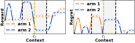
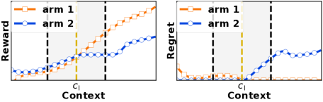
If an arm selection strategy achieves Type-I robustness, the lower bound for the true reward approaches the optimal worst-case reward in the defense region as increases. Therefore, a strategy achieving type-I robustness objective can prevent very low reward. For example, in Fig. 1(a), arm 1 is the one that maximizes the worst-case reward, which is not necessarily optimal but always avoids extremely low reward under any context in the defense region.
Note that maximizing the worst-case reward is equivalent to minimizing the robust regret defined in (Kirschner et al. 2020), which is written using our formulation as
| (7) |
However, this robust regret is a pseudo regret because the rewards of oracle arm and selected arm are compared under different contexts (i.e., their respective worst-case contexts), and it is not an upper or lower bound of the true regret . To obtain a robust regret performance, we need to define another robustness objective based on the true regret.
4.2 Type-II Robustness
To provide robustness for the regret with imperfect context, we can minimize the cumulative worst-case regret, which is expressed as
| (8) |
Clearly, the true regret , and minimizing the worst-case regret is equivalent to minimizing an upper bound for the true regret. Define the instantaneous regret function with respect to context and arm as . Since given the reward function the optimization is decoupled among different rounds, the robust oracle arm to minimize the worst-case regret at round is
| (9) |
For analysis in the following sections, given , the corresponding context for the worst-case regret is denoted as
| (10) |
and the resulting optimal worst-case regret is
| (11) |
Now, we can give the definition of Type-II robustness as follows.
Definition 4.
If, with an arm selection strategy , the difference between the cumulative true regret and the optimal cumulative worst-case regret is sub-linear with respect to , then the strategy achieves Type-II robustness.
If an arm selection strategy achieves Type-II robustness, as time increases, the upper bound for the true regret also approaches the optimal worst-case regret . Hence, a strategy achieving type-II robustness objective can prevent a high regret. As shown in Fig. 1(b), arm 1 is selected by minimizing the worst-case regret, which is a robust arm selection because the regret of arm 1 under any context in the defense region is not too high.
4.3 Comparison of Two Robustness Objectives
The two types of robustness correspond to the algorithms maximizing the worst-case reward and minimizing the worst-case regret, respectively. In many cases, they result in different arm selections. Take the two scenarios in Fig. 1 as examples. In the scenario of Fig. 1(a), given the defense region, arm 1 is selected by maximizing the worst-case reward and arm 2 is selected by minimizing the worst-case regret. It can be observed that the worst-case regrets of the two arms are very close, but the worst-case reward of arm 2 is much lower than that of arm 1. Thus, the strategy of maximizing the worst-case reward is more suitable for this scenario. Differently, in the scenario of Fig. 1(b), arm 2 is selected by maximizing the worst-case reward and arm 1 is selected by minimizing the worst-case regret. Since the worst-case rewards of the two arms are very close and the worst-case regret of arm 2 is much larger than arm 1, it is more suitable to minimize the worst-case regret.
5 Robust Bandit Arm Selection
In this section, we propose two robust arm selection algorithms: (1) (Maximize Minimum Upper Confidence Bound), which aims to maximize the minimum reward (Type-I robustness objective); and (2) (Minimize Worst-case Degradation), which aims to minimize the maximum regret (Type-II robustness objective). We derive the regret and reward bounds for both algorithms and the proofs are available in (Yang and Ren 2021).
5.1 : Maximize Minimum UCB
Algorithm
Analysis
The next theorem gives a lower bound of the cumulative true reward of in terms of the optimal worst-case reward and a sub-linear term.
Theorem 3.
Remark 1.
Theorem 3 shows that by , the difference between the optimal cumulative worst-case reward and the cumulative true reward is sub-linear and thus effectively achieves Type-I robustness according to Definition 3. This means that the reward by has a bounded sub-linear gap compared to the optimal worst-case reward obtained with perfect knowledge of the reward function.
We are also interested in the cumulative true regret of which is given in the following corollary.
Corollary 3.1.
Remark 2.
Corollary 3.1 shows that the worst-case regret by can be quite larger than the optimal worst-case regret given in Eqn. (11) (Type-II robustness objective). Actually, despite being robust in terms of rewards, arms selected by can still have very large regret as shown in Fig. 1(b). Thus, to achieve type-II robustness, it is necessary to develop an arm selection algorithm that minimizes the worst-case regret.
5.2 : Minimize Worst-case Degradation
Algorithm
is designed to asymptotically minimize the worst-case regret. Without the oracle knowledge of reward function, performs arm selection based on the upper bound of regret. Denote referred to as UCB degradation at context . By Lemma 1, the instantaneous true regret can be bounded as
| (15) |
where is called the worst case degradation, and has a vanishing impact by Lemma 2. Thus, to minimize worst-case regret, minimizes its upper bound excluding the vanishing term , i.e.
| (16) |
The context that attains the worst case in Eqn. (16) is written as .
Analysis
Given arm selected by , the next lemma gives an upper bound of worst-case degradation.
Lemma 4.
Then, in order to show that approaches , we need to prove that vanishes as increases. But, this is difficult because the considered sequence is different from the actual sequence of context and selected arms under . To circumvent this issue, we first introduce the concept of covering (Wu 2016). Denote as the context-arm space. If a finite set is an covering of the space , then for each , there exists at least one satisfying . Denote as the cell with respect to . Since the dimension of the entries in is , the size of the is . Besides, we assume the mapping function is Lipschitz continuous, i.e. , . Next, we prove the following proposition to bound the sum of confidence widths under some conditions.
Proposition 5.
Let be the sequence of true contexts and selected arms by bandit algorithms and be the considered sequence of contexts and actions. Suppose that both and belong to . Besides, with an covering , , there exists such that two conditions are satisfied: First, , such that . Second, if at round , for some , then such that . If the mapping function is Lipschitz continuous with constant , the sum of squared confidence widths is bounded as
where is the dimension of , is the effective dimension defined in the proof, and .
Remark 3.
The conditions in Proposition 5 guarantee that the time interval between the events that true context-arm feature lies in the same cell is not larger than , which is proportional to the size of the -covering . That means, similar contexts and selected arms occur in the true sequence repeatedly if is large enough. If contexts are sampled from a bounded space with some distribution, then similar contexts will occur repeatedly. Also, note that the arm in our considered sequence is the UCB-optimal arm, which becomes close to the optimal arm for if the confidence width is sufficiently small. Hence, there exists some context error budget sequence such that, starting from a certain round , the two conditions are satisfied. The two conditions in Proposition 5 are mainly for theoretical analysis of .
Theorem 6.
If is used to select arms with imperfect context and as time goes on, and the conditions in Proposition 5 are satisfied, then for any true context at round , with a probability of , we have the following bound on the cumulative true regret:
where is the optimal worst-case regret for round in Eqn. (11), is the dimension of , is the effective dimension defined in the proof of Proposition 5, is the rank of and is given in Lemma 1.
Remark 4.
Next, in parallel with , we derive the bound of true reward for .
Corollary 6.1.
If is used to select arms with imperfect context and as time goes on, and the true sequence of context and arm obeys the conditions in Proposition 5, then for any true contexts at round , with a probability of , we have the following lower bound of the cumulative reward
where is the optimal worst-case regret for round in Eqn. (11), is the dimension of , is the effective dimension defined in the proof of Proposition 5, is the rank of , and is given in Lemma 1.
Remark 5.
Corollary 6.1 shows that as becomes sufficiently large, the difference between the optimal worst-case reward and the true reward of the selected arm is no larger than the optimal worst-case regret . With perfect context, we have , and hence and both asymptotically maximize the reward, implying that these two types of robustness are the same under perfect context.
5.3 Summary of Main Results
| Algorithms | Regret | Reward |
|---|---|---|
6 Simulation
Edge computing is a promising technique to meet the demand of latency-sensitive applications (Shi et al. 2016). Given multiple heterogeneous edge datacenters located in different locations, which one should be selected? Specifically, each edge datacenter is viewed as an arm, and the users’ workload is context that can only be predicted prior to arm selection. Our goal is to learn datacenter selection to optimize the latency in a robust manner given imperfect workload information. We assume that the service rate of the edge datacenter , , is , the computation latency satisfies an M/M/1 queueing model and the average communication delay between this datacenter and users is . Hence, the average total latency cost can be expressed as which is commonly-considered in the literature (Lin et al. 2011; Xu, Chen, and Ren 2017; Lin et al. 2012). The detailed settings are given in (Yang and Ren 2021).
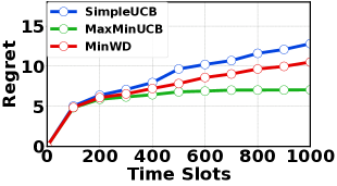
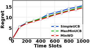
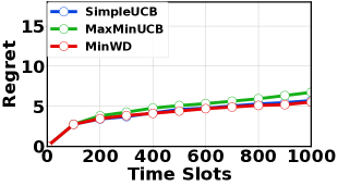
In Fig. 2, we compare different algorithms in terms of three cumulative regret objectives: robust regret in Eqn. (7), worst-case regret in Eqn. (8) and true regret in Eqn. (2). We consider the following algorithms: with imperfect context, with imperfect context and with imperfect context. Given a sequence of true contexts, imperfect context sequence is generated by sampling i.i.d. uniform distribution over at each round. In the simulations, Gaussian kernel with parameter is used for reward (loss) estimation. in Eqn. (3) is set as . The exploration rate is set as .
As is shown in Fig. 2(a), has the best performance of robust regret among the three algorithms. This is because targets at type-I robustness objective which is equivalent to minimizing the robust regret. However, is not the best algorithm in terms of true regret as is shown in Fig. 2(c) since robust regret is not an upper or lower bound of true regret. Another robust algorithm is also better than in terms of robust regret, and it has the best performance among the three algorithms in terms of the worst-case regret, as shown in Fig. 2(b). This is because the regret of approaches the optimal worst-case regret (Theorem 6). also has a good performance of true regret, which coincides with the fact that the worst-case regret is the upper bound of the true regret. By comparing the three algorithms in terms of the three regret objectives, we can clearly see that and achieve performance robustness in terms of the robust regret and worst-case regret, respectively.
7 Conclusion
In this paper, considering a bandit setting with imperfect context, we propose: which maximizes the worst-case reward; and which minimizes the worst-case regret. Our analysis of and based on regret and reward bounds shows that as time goes on, and both perform as asymptotically well as their counterparts that have perfect knowledge of the reward function. Finally, we consider online edge datacenter selection and run synthetic simulations for evaluation.
Acknowledgments
This work was supported in part by the NSF under grants CNS-1551661 and ECCS-1610471.
References
- Abbasi-Yadkori, Pál, and Szepesvári (2011) Abbasi-Yadkori, Y.; Pál, D.; and Szepesvári, C. 2011. Improved Algorithms for Linear Stochastic Bandits. NeurIPS .
- Agrawal and Goyal (2012) Agrawal, S.; and Goyal, N. 2012. Analysis of Thompson Sampling for the Multi-armed Bandit Problem. COLT .
- Agrawal and Goyal (2013) Agrawal, S.; and Goyal, N. 2013. Thompson Sampling for Contextual Bandits with Linear Payoffs. ICML .
- Altschuler, Brunel, and Malek (2019) Altschuler, J.; Brunel, V.-E.; and Malek, A. 2019. Best Arm Identification for Contaminated Bandits. Journal of Machine Learning Research 20(91): 1–39.
- Amazon (2021) Amazon. 2021. Amazon AWS Auto Scaling Documentation. https://docs.aws.amazon.com/autoscaling/.
- Audibert and Bubeck (2009) Audibert, J.; and Bubeck, S. 2009. Minimax policies for adversarial and stochastic bandits. COLT .
- Auer, Cesa-Bianchi, and Fischer (2002) Auer, P.; Cesa-Bianchi, N.; and Fischer, P. 2002. Finite-time Analysis of the Multiarmed Bandit Problem. Machine Learning 47: 235–256.
- Auer et al. (2002) Auer, P.; Cesa-Bianchi, N.; Freund, Y.; and Schapire, R. E. 2002. The Nonstochastic Multiarmed Bandit Problem. SIAM Journal on Computing 32: 48–77.
- Auer and Chiang (2016) Auer, P.; and Chiang, C.-K. 2016. An Algorithm with Nearly Optimal Pseudo-regret for Both Stochastic and Adversarial Bandits. In COLT.
- Bogunovic et al. (2018) Bogunovic, I.; Scarlett, J.; Jegelka, S.; and Cevher, V. 2018. Adversarially Robust Optimization with Gaussian Processes. In NIPS.
- Brockwell et al. (2016) Brockwell, P. J.; Brockwell, P. J.; Davis, R. A.; and Davis, R. A. 2016. Introduction to time series and forecasting. Springer.
- Bubeck and Cesa-Bianchi (2012) Bubeck, S.; and Cesa-Bianchi, N. 2012. Regret analysis of stochastic and nonstochastic multi-armed bandit problems. Foundations and Trends® in Machine Learning 5: 1–122.
- Chen et al. (2014) Chen, B.; Wang, J.; Wang, L.; He, Y.; and Wang, Z. 2014. Robust optimization for transmission expansion planning: Minimax cost vs. minimax regret. IEEE Transactions on Power Systems 29(6): 3069–3077.
- Chen and Xu (2019) Chen, L.; and Xu, J. 2019. Budget-constrained edge service provisioning with demand estimation via bandit learning. IEEE Journal on Selected Areas in Communications 37(10): 2364–2376.
- Chen et al. (2018) Chen, L.; Xu, J.; Ren, S.; and Zhou, P. 2018. Spatio–temporal edge service placement: A bandit learning approach. IEEE Transactions on Wireless Communications 17(12): 8388–8401.
- Chen, Tan, and Zhang (2019) Chen, Y.; Tan, Y.; and Zhang, B. 2019. Exploiting Vulnerabilities of Load Forecasting Through Adversarial Attacks. In e-Energy.
- Chowdhury and Gopalan (2017) Chowdhury, S. R.; and Gopalan, A. 2017. On kernelized multi-armed bandits. ICML .
- Chu et al. (2011) Chu, W.; Li, L.; Reyzin, L.; and Schapire, R. 2011. Contextual bandits with linear payoff functions. NeurIPS .
- Dani et al. (2008) Dani, V.; Hayes, T.; Thomas, P.; and Kakade, S. 2008. Stochastic linear optimization under bandit feedback. COLT .
- Deshmukh, Dogan, and Scott (2017) Deshmukh, A. A.; Dogan, U.; and Scott, C. 2017. Multi-Task Learning for Contextual Bandits. NeurIPS .
- Dudík, Langford, and Li (2011) Dudík, M.; Langford, J.; and Li, L. 2011. Doubly robust policy evaluation and learning. arXiv preprint arXiv:1103.4601 .
- Garcıa and Fernández (2015) Garcıa, J.; and Fernández, F. 2015. A comprehensive survey on safe reinforcement learning. Journal of Machine Learning Research 16(1): 1437–1480.
- Gerchinovitz and Lattimore (2016) Gerchinovitz, S.; and Lattimore, T. 2016. Refined lower bounds for adversarial bandits. NeurIPS .
- Gers, Schmidhuber, and Cummins (2000) Gers, F. A.; Schmidhuber, J.; and Cummins, F. 2000. Learning to Forget: Continual Prediction with LSTM. Neural Computation 12(10): 2451–2471.
- Goldsmith (2005) Goldsmith, A. 2005. Wireless Communications. Cambridge University Press.
- Guan et al. (2020) Guan, Z.; Ji, K.; Bucci Jr, D. J.; Hu, T. Y.; Palombo, J.; Liston, M.; and Liang, Y. 2020. Robust Stochastic Bandit Algorithms under Probabilistic Unbounded Adversarial Attack. In AAAI.
- Han et al. (2020) Han, Y.; Zhou, Z.; Zhou, Z.; Blanchet, J.; Glynn, P. W.; and Ye, Y. 2020. Sequential Batch Learning in Finite-Action Linear Contextual Bandits. arXiv preprint arXiv:2004.06321 .
- Jadbabaie et al. (2015) Jadbabaie, A.; Rakhlin, A.; Shahrampour, S.; and Sridharan, K. 2015. Online optimization: Competing with dynamic comparators. In AISTATS.
- Jiang et al. (2013) Jiang, R.; Wang, J.; Zhang, M.; and Guan, Y. 2013. Two-stage minimax regret robust unit commitment. IEEE Transactions on Power Systems 28(3): 2271–2282.
- Jun et al. (2018) Jun, K.-S.; Li, L.; Ma, Y.; and Zhu, X. 2018. Adversarial Attacks on Stochastic Bandits. In NIPS.
- Kirschner et al. (2020) Kirschner, J.; Bogunovic, I.; Jegelka, S.; and Krause, A. 2020. Distributionally Robust Bayesian Optimization. In AISTATS.
- Kirschner and Krause (2019) Kirschner, J.; and Krause, A. 2019. Stochastic Bandits with Context Distributions. In NeurIPS.
- Lei, Tewari, and Murphy (2014) Lei, H.; Tewari, A.; and Murphy, S. 2014. An actor-critic contextual bandit algorithm for personalized interventions using mobile devices. NeurIPS .
- Li et al. (2010) Li, L.; Chu, W.; Langford, J.; and Schapire, R. E. 2010. A Contextual-bandit Approach to Personalized News Article Recommendation. In WWW.
- Lin et al. (2012) Lin, M.; Liu, Z.; Wierman, A.; and Andrew, L. L. H. 2012. Online algorithms for geographical load balancing. In IGCC.
- Lin et al. (2011) Lin, M.; Wierman, A.; Andrew, L. L. H.; and Thereska, E. 2011. Dynamic right-sizing for power-proportional data centers. In INFOCOM.
- Liu and Shroff (2019) Liu, F.; and Shroff, N. 2019. Data Poisoning Attacks on Stochastic Bandits. In ICML.
- Lu, Pál, and Pál (2010) Lu, T.; Pál, D.; and Pál, M. 2010. Contextual multi-armed bandits. AISTATS .
- Neu and Olkhovskaya (2020) Neu, G.; and Olkhovskaya, J. 2020. Efficient and robust algorithms for adversarial linear contextual bandits. In COLT.
- Nguyen et al. (2020) Nguyen, T.; Gupta, S.; Ha, H.; Rana, S.; and Venkatesh, S. 2020. Distributionally robust bayesian quadrature optimization. In AISTATS.
- Pourbabaee (2020) Pourbabaee, F. 2020. Robust experimentation in the continuous time bandit problem. Economic Theory 1–31.
- Rakhlin and Sridharan (2013) Rakhlin, A.; and Sridharan, K. 2013. Online Learning with Predictable Sequences. In COLT.
- Saxena et al. (2019) Saxena, V.; Jaldén, J.; Gonzalez, J. E.; Bengtsson, M.; Tullberg, H.; and Stoica, I. 2019. Contextual Multi-Armed Bandits for Link Adaptation in Cellular Networks. In Workshop on Network Meets AI & ML (NetAI).
- Shi et al. (2016) Shi, W.; Cao, J.; Zhang, Q.; Li, Y.; and Xu, L. 2016. Edge Computing: Vision and Challenges. IEEE Internet of Things Journal 3(5): 637–646.
- Si et al. (2020a) Si, N.; Zhang, F.; Zhou, Z.; and Blanchet, J. 2020a. Distributional Robust Batch Contextual Bandits. arXiv preprint arXiv:2006.05630 .
- Si et al. (2020b) Si, N.; Zhang, F.; Zhou, Z.; and BlanchetWu, J. 2020b. Distributionally Robust Policy Evaluation and Learning in Offline Contextual Bandits. In ICML.
- Slivkins (2019) Slivkins, A. 2019. Introduction to Multi-Armed Bandits. Foundations and Trends in Machine Learning 12(1-2): 1–286.
- Srinivas et al. (2010) Srinivas, N.; Krause, A.; Kakade, S.; and Seeger, M. 2010. Gaussian process optimization in the bandit setting: no regret and experimental design. ICML .
- Sun, Dey, and Kapoor (2017) Sun, W.; Dey, D.; and Kapoor, A. 2017. Safety-aware algorithms for adversarial contextual bandit. In ICML.
- Syrgkanis, Krishnamurthy, and Schapire (2016) Syrgkanis, V.; Krishnamurthy, A.; and Schapire, R. 2016. Efficient algorithms for adversarial contextual learning. ICML .
- Valko et al. (2013) Valko, M.; Korda, N.; Munos, R.; Flaounas, I.; and Cristianini, N. 2013. Finite-time analysis of kernelised contextual bandits. UAI .
- Wang, Wu, and Wang (2016) Wang, H.; Wu, Q.; and Wang, H. 2016. Learning Hidden Features for Contextual Bandits. CIKM .
- Wu (2016) Wu, Y. 2016. Packing, covering, and consequences on minimax risk. http://www.stat.yale.edu/~yw562/teaching/598/lec14.pdf.
- Wu et al. (2016) Wu, Y.; Shariff, R.; Lattimore, T.; and Szepesvári, C. 2016. Conservative bandits. In ICML.
- Xu, Chen, and Ren (2017) Xu, J.; Chen, L.; and Ren, S. 2017. Online Learning for Offloading and Autoscaling in Energy Harvesting Mobile Edge Computing. IEEE Transactions on Cognitive Communications and Networking 3(3): 361–373.
- Yang and Ren (2021) Yang, J.; and Ren, S. 2021. Robust Bandit Learning with Imperfect Context. arXiv preprint arXiv:2102.05018 .
- Zhu et al. (2018) Zhu, F.; Guo, J.; Li, R.; and Huang, J. 2018. Robust actor-critic contextual bandit for mobile health (mhealth) interventions. In Proceedings of the 2018 ACM International Conference on Bioinformatics, Computational Biology, and Health Informatics, 492–501.
Appendix A Applications and Simulation Settings
A key novelty of our work is the consideration of imperfect context for arm selection, which characterizes many practical applications such as resource management problems where the true context is difficult to obtain for arm selection until revealed later. We list some examples of these applications in this section and provide the simulation settings.
A.1 Motivating Applications
Cloud Resource Management. Cloud computing platforms are crucial infrastructures offering utility-style computation resources to users on demand. To optimize the performance metrics such as latency and cost for these applications, efficient online cloud resource management such as dynamic virtual machine scheduling is necessary. Contextual bandit learning can be employed in this scenario where the exact workload information (measured in, e.g., how many requests will arrive per unit time) is crucial context information, but cannot be known until the workload actually arrives. Instead, the agent can only predict the upcoming workload by exploiting the recent workload history plus other applicable system features. A real-word example is Amazon’s predictive scaling that leverages time series prediction to estimate upcoming workload for virtual machine scheduling (Amazon 2021). In this motivating example, the context prediction error comes primarily from the workload predictor.
Energy Scheduling in Smart Grid. Energy load is a crucial context information for energy scheduling in smart grid. However, a recent study (Chen, Tan, and Zhang 2019) shows that the energy load predictor in smart grid can be adversarially attacked to produce load estimates (i.e., context for energy scheduling) with higher-than-normal errors. Thus, our model also captures a novel adversarial setting where erroneously predicted context is presented to the agent for arm selection. This example shows that the use of machine learning-based predictor for acquiring context to facilitate the agent’s arm selection can also open a new attack surface — an outside attacker may adversarially modify the predicted context — which requires a robust algorithm with a provable worst-case performance guarantee.
Online Edge Datacenter Selection. With the rapidly increasing number of devices at the Internet edge, computational demand by latency-sensitive applications (e.g., assisted driving and virtual reality) has been escalating. Edge computing is a promising solution to meet the demand, which deploys computation resources at densely-distributed edge datacenters close to end users and thus reduces the overall latency (Shi et al. 2016). Since users’ workloads can be processed in multiple edge datacenters, dynamic selection of edge datacenters plays a key role for minimizing the overall latency — given multiple heterogeneous edge datacenters located in different locations, which one should be selected? Here, servers in each edge datacenter can be either virtual machines rented from third-party service providers or physical servers owned by the edge computing provider itself. We refer to this problem as online edge datacenter selection. Our considered bandit setting applies to the problem of online edge datacenter selection. Specifically, each edge datacenter is viewed as an arm, and the users’ workload is context that can only be predicted prior to arm selection. Our goal is to dynamically select edge datacenters to optimize the latency in a robust manner given imperfect information about users’ workloads.
A.2 Simulation Settings in Section 6
In our simulation, we apply our algorithms to online edge datacenter selection in the context of edge computing. We consider users’ workloads can be processed in one of four available edge datacenters, each having different computation capabilities and communication latencies. Here, we consider a simple latency model to capture first-order effects. Concretely, we assume that the service rate of the edge datacenter , , is , the computation latency satisfies an M/M/1 queueing model and the average communication delay between this datacenter and users is . The values of and are shown in Table 2. In the simulations, perfect context sequence is generated by sampling i.i.d. uniform distribution between 10 and 30 for each round, while the defense budget is set as 2. The average total latency cost can be expressed as
| (18) |
whose inverse can be equivalently viewed as the reward in our model.
| Datacenter | I | II | III | IV |
|---|---|---|---|---|
| 35 | 38 | 45 | 51 | |
| 0.04 | 0.05 | 0.074 | 0.088 |
While we use the simple latency model in Eqn. (18) for generating the ground-true cost, the function form and parameters (e.g., ) may not be known to the agent and needs to be learnt based on latency feedback and revealed context. Note that some practical factors (e.g., workload parallelism) are beyond the scope of our analysis and incorporating them into our simulation does not add substantially to our main contribution.
Appendix B Algorithm and Proofs Related to SimpleUCB
B.1 Algorithm of
We describe in Algorithm 2.
B.2 Proof of Lemma 1
Lemma 1 Assume that the reward function satisfies , the noise satisfies a sub-Gaussian distribution with parameter , and kernel ridge regression is used to estimate the reward function. With a probability of at least , for all and , the estimation error satisfies where , and is the rank of . Let , the squared confidence width is given by .
Proof.
Let be the mapping function with respect to . Define with the th row as and thus . Denote as the collected rewards and the noise vector , so . Then we have
| (19) |
where is an identity matrix with dimensions and the last inequality comes from triangle inequality.
Let and define . By Woodbury formula, we can write by kernel functions:
| (20) |
For the first term of Eqn. (19), using Woodbury formula, we have
| (21) |
where the inequality comes from Cauchy-Schwartz inequality and .
For the second term, we have the following inequalities.
| (22) |
where the first inequality comes from Cauchy-Schwartz inequality.
Since satisfies -sub-Gaussain distribution conditioned on , by Theorem 1 in (Abbasi-Yadkori, Pál, and Szepesvári 2011), with probability , for and , we have
| (23) |
where where is the dimension of the inequality comes from Lemma 10 in (Abbasi-Yadkori, Pál, and Szepesvári 2011).
Combining the bounds of the first and second term in Eqn. (19) and let , we obtain the concentration bound in Lemma 3.1: . ∎
B.3 Proof of Lemma 2
Lemma 2 The confidence widths given for satisfies , where and is the rank of , and so .
Proof.
By Lemma 11 in (Abbasi-Yadkori, Pál, and Szepesvári 2011), if , we have
| (24) |
where . By Hölder’s inequality, we have
| (25) |
∎
Appendix C Proofs Related to
C.1 Proof of Theorem 3
Theorem 3 If is used to select arms with imperfect context, then for any true contexts at round , with a probability of , we have the following lower bound on the worst-case cumulative reward
| (26) |
where is the optimal worst-case reward in Eqn. (6), is the rank of and is given in Lemma 1.
Proof.
By Lemma 1 and UCB defined in Definition 1, with probability , , the instantaneous regret can be bounded as
| (27) |
where the last inequality comes from the arm selection policy of implying that .
With the definition of the optimal worst-case reward and exploiting the arm selection policy of , we can further bound the instantaneous reward as below.
| (28) |
where is the optimal arm for maximizing the worst-case reward defined in Definition 1, , the second inequality comes from the arm selection strategy of such that , the third inequality holds because the definition of in Eqn. (6). which guarantees , and the last inequality comes from Lemma 1 which guarantees . Therefore, combined with Lemma 2, we can get the bound the cumulative reward of . ∎
C.2 Proof of Corollary 3.1
Corollary 3.1 If is used to select arms with imperfect context, then for any true contexts at round , with a probability of , we have the following bound on the cumulative true regret defined in Eqn. (2):
| (29) |
where , is the optimal worst-case reward in Eqn. (6), is the rank of and is given in Lemma 1 .
Appendix D Proofs Related to
D.1 Proof of Lemma 4
Lemma 4 If is used to select arms with imperfect context, then for each , with a probability at least , we have
| (31) |
where is the optimal worst-case regret defined in Eqn. (11), is the context that maximizes the degradation given the arm defined for the optimal worst-case regret in Eqn. (10).
Proof.
Recall that in Eqn. (9), the optimal arm for minimizing the worst-case regret is . By the arm selection policy of , is th arm that minimizes , so the worst-case degradation can be bounded as follows.
| (32) |
where , the second inequality holds because where is the optimal worst-case regret defined in Eqn. (11) and the third inequality is from Lemma 1 which guarantees that and . ∎
D.2 Proof of Proposition 5
We first bound the confidence width sum of considered context-arm sequence in the Lemma 7 assuming a linear reward function, i.e. , and context-arm space is finite with size . Then in Lemma 8, we prove the bound for linear reward case and continuous context-arm space. Finally we generalize the bound to the kernel cases. For conciseness, denote as the true context and selected arm at round and as the considered context and arm at round .
Lemma 7 (Sum of Confidence Width with Finite Context-arm Space).
Let be the sequence of true contexts and selected arms by bandit algorithms and be the considered sequence of contexts and arms. Suppose that both and belong to a finite set with size . Besides, , , two conditions are satisfied. First, such that . Second, if at round , , then , such that . The sum of confidence width is bounded as
| (33) |
where and .
Proof.
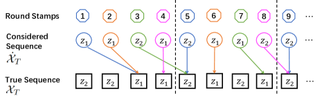
Let . Divide the round stamp sequence uniformly into groups, each with elements. The th group of round stamps, , is , and is a subset of with the first entries. A simple example of group construction is shown in Fig. 3.
Let , for . For the sequence , by Lemma 2, we have where and .
Let’s consider the sequence in . The two conditions in Lemma 8, imply that for and its index , , if , there exists such that the true context-arm (For example, in Fig. 3, is in , and there exists such that ). Therefore we have , and we conclude that . Thus, considering and are both positive definite matrices, we have and . Therefore, for group (), we have
| (34) |
From the above analysis, since , we can get
| (35) |
where the second inequality comes from Lemma 11 in (Abbasi-Yadkori, Pál, and Szepesvári 2011). thus completing the proof. ∎
If the context-arm space is continuous, the finite set assumption of in Lemma 7 is not satisfied anymore. To overcome this issue, we construct an - covering for the context-arm space such that for each , there exists at least one satisfying . Since the dimension of is , the size of the - covering is . Now we can bound the sum of confidence width with linear reward function and continuous context-arm space in Lemma 8.
Lemma 8 (Sum of Confidence Width with Continuous Context-arm Space).
Let be the sequence of true contexts and selected arms by bandit algorithms and be the considered sequence of contexts and actions. Suppose that both and belong to . Besides, with an covering , , there exists such that two conditions are satisfied for . First, , such that . Second, if at round , for some , then such that . The sum of squared confidence width is bounded as
| (36) |
where and .
Proof.
Based on the - covering , we divide the round stamp sequence uniformly into groups, each with elements. The th group is , and is a subset of with the first entries.
Now we consider the th group. The two conditions in this lemma imply that for a certain and its index , , if for some , there exists such that the true context-arm . Denote mapping to its corresponding , and we have . Also, denote , and we have . Let , for . By the above analysis, we have , and so considering and are both positive definite matrices.
By Lemma 2, for the sequence , we have . Denote . Since and belong to the same cell in covering , we have by triangle inequality. Therefore for group , we have
| (37) |
where the first inequality comes from Cauchy-Schwartz inequality and the second inequality holds because and , and the last inequality holds by Lemma 2.
Now we can bound the sum of the confidence widths for the whole sequence as
| (38) |
where the last inequality holds because by Lemma 11 in (Abbasi-Yadkori, Pál, and Szepesvári 2011) and . Let , i.e. , then we have
| (39) |
thus completing the proof. ∎
Now we can prove proposition 5 by generalizing Lemma 8 into kernel case assuming the mapping function is Lipschitz continuous with constant , i.e. , .
Proof of Proposition 5
Proposition 5 Let be the sequence of true contexts and selected arms by bandit algorithms and be the considered sequence of contexts and actions. Suppose that both and belong to . Besides, with an covering , , there exists such that two conditions are satisfied. First, , such that . Second, if at round , for some , then such that . If the mapping function is Lipschitz continuous with constant , the sum of squared confidence widths is bounded as
| (40) |
where is the dimension of , is the effective dimension defined in the proof, and .
Proof.
With the same method in Lemma 8, we construct groups, each with elements. Define , same as Lemma 8 and let , for . By Lemma 8, we have , and so . Therefore for group , we have
| (41) |
where the first inequality comes from Cauchy-Schwartz inequality and the second inequality holds because , and Lipschitz continuity of such that , and the last inequality holds by Lemma 2.
For kernel case, with containing for , we have , where is the rank of . Define the effective dimension as . Then we can bound the sum of the confidence widths for the whole sequence as
| (42) |
Let , i.e. , then we have
| (43) |
thus completing the proof. ∎
D.3 Proof of Theorem 6
Theorem 6. If is used to select arms with imperfect context and as time goes on, and the conditions in Proposition 5 are satisfied, then for any true context at round , with a probability of , we have the following bound on the cumulative true regret:
where is the optimal worst-case regret for round in Eqn. (11), is the dimension of , is the effective dimension defined in the proof of Proposition 5, is the rank of and is given in Lemma 1.
Proof.
Since with a probability , , , we can bound the cumulative regret of as
| (44) |
where the second inequality comes from Lemma 4.
D.4 Proof of Corollary 6.1
Corollary 6.1 If is used to select arms with imperfect context and as time goes on, and the true sequence of context and arm obeys the conditions in Proposition 5, then for any true contexts at round , with a probability of , we have the following lower bound of the cumulative reward
where is the optimal worst-case regret for round in Eqn. (11), is the dimension of , is the effective dimension defined in the proof of Proposition 5, is the rank of , and is given in Lemma 1.
Proof.
By Lemma 1, with a probability , , we can bound the reward as below
| (46) |
Recall that the upper bound of the worst-case degradation is defined as , so the reward can be further bounded as
| (47) |
where the last inequality is because by max-min inequality.
Note that is the arm selection policy of whose solutions are and . This observation is important since it bridges and . Also, recall that in Eqn. (4), is the optimal arm for worst-case reward and is the optimal worst-case reward. Then following Eqn. (47), we have
| (48) |
where , the second inequality holds by the arm selection strategy of such that , the third inequality comes from the definition of in Eqn. (6) which guarantees and the forth inequality comes from Lemma 1 such that .
Finally, since is the upper bound of instantaneous regret of , by directly using Theorem 6 we can prove the lower bound reward of . ∎