Infrared facets of the three-gluon vertex

Abstract

We present novel lattice results for the form factors of the quenched three-gluon vertex of QCD, in two special kinematic configurations that depend on a single momentum scale. We consider three form factors, two associated with a classical tensor structure and one without tree-level counterpart, exhibiting markedly different infrared behaviors. Specifically, while the former display the typical suppression driven by a negative logarithmic singularity at the origin, the latter saturates at a small negative constant. These exceptional features are analyzed within the Schwinger-Dyson framework, with the aid of special relations obtained from the Slavnov-Taylor identities of the theory. The emerging picture of the underlying dynamics is thoroughly corroborated by the lattice results, both qualitatively as well as quantitatively.

1 Introduction

The three-gluon vertex is a central component of QCD [1, 2, 3], being intimately linked to a variety of fundamental nonperturbative phenomena, and the scrutiny of its properties has received considerable attention in recent years [4, 5, 6, 7, 8, 9, 10, 11, 12, 13, 14, 15, 16, 17, 18, 19, 20, 21, 22, 23]. A particularly noteworthy feature of this vertex in the Landau gauge is the infrared behavior of the form factors associated with the classical (tree-level) tensorial structures. Specifically, as the space-like momenta decrease from the ultraviolet to the infrared regime, the size of these form factors is gradually reduced, displaying the so-called “infrared suppression” [5, 6, 7, 8, 9, 10, 11, 12, 13, 14, 15, 16, 17, 18, 19, 20, 21, 22]. This suppression culminates with the manifestation of a logarithmic divergence at the origin, which drives the form factors to negative infinity  [9, 16, 19, 20, 21, 22]

As has been explained in detail in the recent literature, this special behavior of the vertex originates from the interplay between dynamical effects occurring in the two-point sector of QCD [20, 21, 22]. In particular, while the gluon acquires dynamically an effective mass [24, 25, 26, 27, 28], responsible for the infrared saturation of the Landau-gauge gluon propagator [29, 30, 31, 32, 33, 34, 35, 36, 37, 38, 39, 40, 41, 42, 43, 44, 45, 46, 47], the ghost remains massless even nonperturbatively [48, 49, 36, 37, 50]. As a result, loop diagrams containing ghost propagators furnish infrared divergent logarithms, while gluonic loops, being “protected” by the mass, are infrared finite.

The formalism obtained from the fusion of the Pinch Technique [24, 51, 52, 53] with the Background Field Method (PT-BFM) [54], known as “PT-BFM” scheme [53, 35, 55], is particularly suitable for exposing this interplay, by combining the Schwinger-Dyson equations (SDEs) with the Slavnov-Taylor identity (STI) satisfied by the three-gluon vertex [1, 2, 3, 56].

In the present work we employ this scheme to scrutinize further this dynamical picture, through the analysis of new results from quenched lattice simulations for three vertex form factors, defined in two special kinematic configurations that involve a single momentum scale.

In particular, in the case of the two “classical” form factors simulated, a considerable increase in the statistics permits us to obtain a cleaner signal of the infrared divergences that they display, and accurately determine their strength. This new information, in turn, enables us to probe more stringently, at the quantitative level, the underlying mechanisms associated with their emergence.

In addition, we present for the first time lattice results for a form factor that has no classical analogue. The dynamics of this purely quantum contribution may be described by means of the corresponding SDE, and, in contradistinction to the classical form factors, does not display any infrared divergences. The data obtained corroborate this prediction, being completely compatible with a finite rather than a divergent contribution at low momenta.

2 General considerations and theoretical setup

Our point of departure is the three-point correlation function composed by SU(3) gauge fields, $\widetilde{A}^{a}_{\alpha}(q)$, in Fourier space,

$${\cal G}_{\alpha\mu\nu}^{abc}(q,r,p)\ =\ \langle\widetilde{A}^{a}_{\alpha}(q)\widetilde{A}^{b}_{\mu}(r)\widetilde{A}^{c}_{\nu}(p)\rangle\ =\ f^{abc}{\cal G}_{\alpha\mu\nu}(q,r,p)\,,$$ (1)

with $q+r+p=0$.  ${\cal G}_{\alpha\mu\nu}^{abc}(q,r,p)$ may be cast in the form

$${\cal G}_{\alpha\mu\nu}(q,r,p)=g\overline{\Gamma}_{\alpha\mu\nu}(q,r,p)\Delta(q^{2})\Delta(r^{2})\Delta(p^{2})\ ,$$ (2)

where we have introduced the transversally projected vertex [21, 22],

$$\overline{\Gamma}_{\alpha\mu\nu}(q,r,p)\ =\ {\rm{I}}\!\Gamma^{\alpha^{\prime}\mu^{\prime}\nu^{\prime}}(q,r,p)P_{\alpha^{\prime}\alpha}(q)P_{\mu^{\prime}\mu}(r)P_{\nu^{\prime}\nu}(p)\ ,$$ (3)

with ${\rm{I}}\!\Gamma$ denoting the usual one-particle irreducible (1PI) three-gluon vertex. In addition, $g$ is the gauge coupling, and $\Delta(q^{2})$ the scalar component of the gluon propagator,

$$\Delta^{ab}_{\mu\nu}(p)=\langle\widetilde{A}^{a}_{\mu}(p)\widetilde{A}^{b}_{\mu}(-p)\rangle=\Delta(p^{2})\delta^{ab}P_{\mu\nu}(p)\,,$$ (4)

with $P_{\mu\nu}(p)=g_{\mu\nu}-p_{\mu}p_{\nu}/p^{2}$, the standard transverse projector. Evidently, $q^{\alpha}{\cal G}_{\alpha\mu\nu}=r^{\mu}{\cal G}_{\alpha\mu\nu}=p^{\nu}{\cal G}_{\alpha\mu\nu}=0$.

The typical quantity studied in Landau-gauge lattice simulations is the projection [16, 17, 19]

$$L(q,p,r;\lambda)=\frac{{\cal G}_{\alpha\mu\nu}(q,r,p)\lambda^{\alpha\mu\nu}(q,r,p)}{\rule[0.0pt]{0.0pt}{12.80365pt}\lambda_{\alpha\mu\nu}(q,r,p)\lambda^{\alpha\mu\nu}(q,r,p)}\rule[0.0pt]{0.0pt}{14.22636pt}\;,$$ (5)

where $\lambda^{\alpha\mu\nu}$ is a transverse tensor whose form should be appropriately chosen, depending on the kinematic configuration employed and the form factor that one wants to extract. In what follows we will focus our attention on the (i) totally symmetric and (ii) asymmetric configurations of the three-gluon vertex.

In case (i), the momenta configuration is defined by $q^{2}=p^{2}=r^{2}:=s^{2}$, such that $q\cdot r=q\cdot r=r\cdot p=-s^{2}/2$ and $\theta=\widehat{qr}=\widehat{qp}=\widehat{rp}=2\pi/3$. The tensor structure of $\overline{\Gamma}$ is then reduced down to [57, 58]

$$\overline{\Gamma}^{\alpha\mu\nu}(q,r,p)=\overline{\Gamma}^{\rm sym}_{1}(s^{2})\,\lambda_{1}^{\alpha\mu\nu}(q,r,p)+\overline{\Gamma}^{\rm sym}_{2}(s^{2})\,\lambda_{2}^{\alpha\mu\nu}(q,r,p)\,,$$ (6)

with the two tensors

$$\lambda_{1}^{\alpha\mu\nu}(q,r,p) =\overline{\Gamma}_{0}^{\alpha\mu\nu}(q,r,p)\,,$$ (7a)

$$\lambda_{2}^{\alpha\mu\nu}(q,r,p) =\frac{(q-r)^{\nu}(r-p)^{\alpha}(p-q)^{\mu}}{s^{2}}\ ;$$ (7b)

$\overline{\Gamma}_{0}^{\alpha\mu\nu}(q,r,p)$ is the tree-level version of the vertex in Eq. (3).

We next project out of $L$ two particular combinations, denoted by $T_{i}^{\rm sym}$, each containing one of the $\overline{\Gamma}_{i}^{\rm sym}$, namely

$$T^{\rm sym}_{i}(s^{2}):=g\overline{\Gamma}^{\rm sym}_{i}(s^{2})\Delta^{3}(s^{2})=\left.L\left(\mkern 2.0mu\overline{\mkern-3.5mu\lambda\mkern-1.2mu}\mkern 1.2mu_{i}\right)\rule[0.0pt]{0.0pt}{8.5359pt}\right|_{q^{2}=r^{2}=p^{2}:=s^{2}}\;,$$ (8)

where

$$\mkern 2.0mu\overline{\mkern-3.5mu\lambda\mkern-1.2mu}\mkern 1.2mu_{i}^{\alpha\mu\nu}(q,r,p)\ =\ \sum_{j=1}^{2}\beta_{ij}\,\lambda_{j}^{\alpha\mu\nu}(q,r,p)\;,$$ (9)

with $\beta_{11}=1$,  $\beta_{12}=1/2$,   $\beta_{21}=6/11$, and $\beta_{22}=1$, such that

$$\mkern 2.0mu\overline{\mkern-3.5mu\lambda\mkern-1.2mu}\mkern 1.2mu_{i\,\alpha\mu\nu}(q,r,p)\,\lambda_{j}^{\alpha\mu\nu}(q,r,p)\ =\ \delta_{ij}\,\mkern 2.0mu\overline{\mkern-3.5mu\lambda\mkern-1.2mu}\mkern 1.2mu_{i\,\alpha\mu\nu}(q,r,p)\,\mkern 2.0mu\overline{\mkern-3.5mu\lambda\mkern-1.2mu}\mkern 1.2mu_{i}^{\alpha\mu\nu}(q,r,p)\ .$$ (10)

In case (ii), the asymmetric configuration corresponds to the kinematic limit $p\to 0$, $r=-q$ and $\theta=\widehat{qr}=\pi$. In these kinematics we have [59]

$$\overline{\Gamma}^{\alpha\mu\nu}(q,-q,0)=\overline{\Gamma}_{3}^{\rm asym}(q^{2})\lambda_{3}^{\alpha\mu\nu}(q,-q,0)\;,$$ (11)

in terms of the single tensor,

$$\lambda_{3}^{\alpha\mu\nu}(q,-q,0)=2q^{\nu}P^{\alpha\mu}(q)\,,$$ (12)

which emerges after the implementation of the asymmetric limit on the tensorial basis of the three-gluon vertex.

A careful analysis reveals that the projection of $\overline{\Gamma}^{\rm asym}_{3}$ from $L$ proceeds through contraction by $\lambda_{3}^{\alpha\mu\nu}(q,-q,0)$ itself, namely

$$T^{\rm asym}_{3}(q^{2})=g\overline{\Gamma}^{\rm asym}_{3}(q^{2})\Delta^{2}(q^{2})\Delta(0)=\left.L\left(\lambda_{3}\right)\rule[0.0pt]{0.0pt}{8.5359pt}\right|_{r^{2}=q^{2};p^{2}\to 0}\;.$$ (13)

Note that the limit $p\to 0$ is path-independent, i.e., does not depend on the angle formed between $p$ and $q$.

We next implement multiplicative renormalization by introducing the standard renormalization constants, $Z_{i}$, relating bare and renormalized quantities as

$$\Delta_{R}(q^{2}) =Z_{A}^{-1}\Delta(q^{2}), {\cal G}_{R}(q,r,p) =Z_{A}^{-3/2}{\cal G}(q,r,p),$$

$$g_{R} =Z_{A}^{3/2}Z_{3}^{-1}g, \overline{\Gamma}_{R}(q,r,p) =Z_{3}\overline{\Gamma}(q,r,p)\,.$$ (14)

Within the momentum subtraction (MOM) scheme [60] that we use, the renormalized correlation functions must acquire their tree-level expressions at the subtraction point $\mu^{2}$, e.g., $\Delta^{-1}_{{\rm R}}(\mu^{2})=\mu^{2}$.

Turning to the kinematic configurations (i) and (ii), we impose, correspondingly, the MOM conditions

$$\overline{\Gamma}_{1\,{\rm R}}^{\rm sym}(\mu^{2})\ =\ 1\,,\qquad\overline{\Gamma}_{3\,{\rm R}}^{\rm asym}(\mu^{2})\ =\ 1\,,$$ (15)

which define the symmetric and asymmetric MOM schemes, respectively [57, 61, 58, 59].

Focusing on case (i), we want to express $\overline{\Gamma}_{{\rm R}\,i}^{\rm sym}(s^{2})$ exclusively in terms of the bare lattice quantities $\Delta$ and $T^{\rm sym}_{i}$. This may be readily accomplished, since multiplicative renormalization entails that, for any correlation function $G(q^{2})$, the ratio $G(q^{2}_{1})/G(q^{2}_{2})=G_{R}(q^{2}_{1})/G_{R}(q^{2}_{2})$ is a renormalization-group invariant combination.

In particular, forming the ratio $T^{\rm sym}_{i}(s^{2})/T_{1}^{\rm sym}(\mu^{2})$ using Eq. (8), and employing the condition of Eq. (15), we find

$$\overline{\Gamma}_{i\,{\rm R}}^{\rm sym}(s^{2})=\frac{T^{\rm sym}_{i}(s^{2})}{T^{\rm sym}_{1}(\mu^{2})}\,\left(\frac{\Delta(\mu^{2})}{\Delta(s^{2})}\right)^{3}\quad\mbox{with}\quad i=1,2\,.$$ (16)

Applying exactly analogous reasoning to the case (ii), we obtain

$$\overline{\Gamma}_{3\,{\rm R}}^{\rm asym}(q^{2})=\frac{T^{\rm asym}_{3}(q^{2})}{T^{\rm asym}_{3}(\mu^{2})}\,\left(\frac{\Delta(\mu^{2})}{\Delta(q^{2})}\right)^{2}\,.$$ (17)

From this point on, we drop the subscript “${\rm R}$” from the renormalized $\overline{\Gamma}_{i}$.

3 Connecting the two- and three-point sectors of QCD

In this section we present the salient features of PT-BFM approach, pertinent to the the gluon propagator and three gluon vertex. The upshot of these considerations is the derivation of theoretical expressions for the form factors $\overline{\Gamma}_{i}$, which will be contrasted with the new lattice results in the next section.

Within the PT-BFM framework it is natural to cast the infrared finite $\Delta(q^{2})$ as the sum of two distinct pieces [62] ,

$$\Delta^{-1}(q^{2})=q^{2}J(q^{2})+m^{2}(q^{2})\,,$$ (18)

where $J(q^{2})$ denotes the so-called “kinetic term”, while $m^{2}(q^{2})$ represents a momentum-dependent mass scale. Clearly, $m^{2}(0)=\Delta^{-1}(0)$ is the saturation point of the gluon propagator.

The emergence of $m^{2}(q^{2})$ hinges crucially on the structure of ${\rm{I}}\!\Gamma_{\alpha\mu\nu}$, entering in the SDE for $\Delta(q^{2})$. In particular, ${\rm{I}}\!\Gamma_{\alpha\mu\nu}$ must be decomposed as

$${\rm{I}}\!\Gamma_{\alpha\mu\nu}(q,r,p)=\Gamma_{\alpha\mu\nu}(q,r,p)+V_{\alpha\mu\nu}(q,r,p)\,,$$ (19)

where $V_{\alpha\mu\nu}$ is comprised by longitudinally coupled massless poles, i.e. $P^{\alpha}_{\alpha^{\prime}}(q)P^{\mu}_{\mu^{\prime}}(r)P^{\nu}_{\nu^{\prime}}(p)V_{\alpha\mu\nu}(q,r,p)=0$, and $\Gamma_{\alpha\mu\nu}$ denotes the pole-free part of the vertex. By virtue of the above property, $V_{\alpha\mu\nu}$ drops out from the $\overline{\Gamma}_{\alpha\mu\nu}$ in Eq. (3), and, consequently, the lattice projection of Eq. (5) depends only on $\Gamma_{\alpha\mu\nu}$.

$\Gamma^{\alpha\mu\nu}(q,r,p)$ is usually decomposed into a longitudinal and a transverse contribution [2, 3, 20, 22]

$$\Gamma^{\alpha\mu\nu}(q,r,p)\ =\ \Gamma_{L}^{\alpha\mu\nu}(q,r,p)+\Gamma_{T}^{\alpha\mu\nu}(q,r,p)\;,$$ (20)

with $q_{\alpha}\Gamma_{T}^{\alpha\mu\nu}(q,r,p)=r_{\mu}\Gamma_{T}^{\alpha\mu\nu}(q,r,p)=p_{\nu}\Gamma_{T}^{\alpha\mu\nu}(q,r,p)=0$.

Their tensorial decomposition in the basis of [2, 3, 20], reads

$$\Gamma_{L}^{\alpha\mu\nu}(q,r,p) =\sum_{i=1}^{10}X_{i}(q^{2},r^{2},p^{2})\,\ell_{i}^{\alpha\mu\nu}(q,r,p)\;,$$ (21a)

$$\Gamma_{T}^{\alpha\mu\nu}(q,r,p) =\ \sum_{i=1}^{4}Y_{i}(q^{2},r^{2},p^{2})\,t_{i}^{\alpha\mu\nu}(q,r,p)\;,$$ (21b)

where the explicit form of the basis tensors $\ell_{i}$ and $t_{i}$ is given in Eqs. (3.4) and (3.5) of [20].

Note that the tree-level expression for $\Gamma^{\alpha\mu\nu}$ is recovered from Eq. (21a) by setting $X_{1}=X_{4}=X_{7}=1$, and $X_{i}$ = 0 for all remaining terms.

Using the above decomposition, one may express the $\overline{\Gamma}_{i}$ in terms of the $X_{i}$ and $Y_{i}$. Specifically, in Euclidean space, we obtain

$$\overline{\Gamma}_{1}^{\rm sym}(s^{2}) = X_{1}(s^{2})-\frac{s^{2}}{2}X_{3}(s^{2})+\frac{s^{4}}{4}Y_{1}(s^{2})-\frac{s^{2}}{2}Y_{4}(s^{2})\,,$$

$$\overline{\Gamma}_{2}^{\rm sym}(s^{2}) = \frac{3s^{2}}{4}X_{3}(s^{2})-\frac{3s^{4}}{8}Y_{1}(s^{2})-\frac{s^{2}}{4}Y_{4}(s^{2})\,,$$ (22)

where $X_{i}(s^{2})\equiv X_{i}(s^{2},s^{2},s^{2})$ and $Y_{i}(s^{2})\equiv Y_{i}(s^{2},s^{2},s^{2})$. Moreover, one has

$$\overline{\Gamma}^{\rm asym}_{3}(q^{2})=X_{1}(q^{2},q^{2},0)-q^{2}X_{3}(q^{2},q^{2},0)\;.$$ (23)

Past this point, we will determine the $X_{i}$ by resorting to a construction relying on the STIs satisfied by ${\rm{I}}\!\Gamma_{\alpha\mu\nu}$, i.e. ,

$$p^{\nu}{\rm{I}}\!\Gamma_{\alpha\mu\nu}(q,r,p)=F(p^{2})[{\cal T}_{\mu\alpha}(r,p,q)-{\cal T}_{\alpha\mu}(q,p,r)]\,,$$ (24)

with

$${\cal T}_{\mu\alpha}(r,p,q):=\Delta^{-1}(r^{2})P_{\mu}^{\sigma}(r)H_{\sigma\alpha}(r,p,q)\,.$$ (25)

$F(p^{2})$ denotes the ghost dressing function, while $H_{\nu\mu}(q,p,r)$ is the ghost-gluon scattering kernel [2, 3, 63], whose tensorial decomposition is given by [$A_{i}\equiv A_{i}(q,p,r)$]

$$H_{\nu\mu}(q,p,r)=g_{\nu\mu}A_{1}+q_{\mu}q_{\nu}A_{2}+r_{\mu}r_{\nu}A_{3}+q_{\mu}r_{\nu}A_{4}+r_{\mu}q_{\nu}A_{5}\,.$$ (26)

The decompositions given in Eqs. (18) and (19) prompt the separation of the above STI into two “partial” STIs, obtained by implementing the matching $\Gamma\leftrightarrow J$ and $V\leftrightarrow m^{2}$ [64, 62]. Based on this hypothesis, one may extend the BC construction of [2] to the case of infrared finite gluon propagator, expressing the $X_{i}$ in terms of the $J$, the $F$, and the $A_{i}$. In particular, we obtain

$$X_{1}(s^{2}) =Z_{1}^{\rm sym}F(s^{2})J(s^{2})R_{1}^{\rm sym}(s^{2})\,,$$

$$X_{3}(s^{2}) =Z_{1}^{\rm sym}F(s^{2})\left[J^{\prime}(s^{2})R_{2}^{\rm sym}(s^{2})+J(s^{2})R_{3}^{\rm sym}(s^{2})\right]\,,$$ (27)

and

$$X_{1}(q^{2},q^{2},0) =Z_{1}^{\rm asym}F(q^{2})J(q^{2})R_{1}^{\rm asym}(q^{2})\,,$$ (28)

$$X_{3}(q^{2},q^{2},0) =Z_{1}^{\rm asym}F(0)\left[J^{\prime}(q^{2})R_{2}^{\rm asym}(q^{2})+J(q^{2})R_{3}^{\rm asym}(q^{2})\right]\,,$$

where the $R_{j}^{\rm sym}$ and $R_{j}^{\rm asym}$ are linear combinations of the $A_{i}$ and their derivatives, whereas $Z_{1}^{\rm sym}$ and $Z_{1}^{\rm asym}$ are, respectively, the finite renormalization constants [65] of the ghost-gluon kernel in the symmetric and asymmetric MOM schemes, defined in Eq. (15).

Note that this procedure leaves the transverse vertex form factors $Y_{i}$ undetermined; nonetheless, as we will see in the next section, their qualitative features may be deduced from the corresponding SDE governing the vertex $\Gamma$.

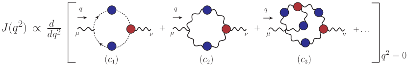
Figure 1: SDE diagrams contributing to the derivative of the gluon propagator at the origin. Blue (red) circles indicate fully dressed propagators (vertices).

The ingredients comprising Eqs. (27) and (28) are obtained as follows. $R_{j}^{\rm sym}$ and $R_{j}^{\rm asym}$ may be computed using the SDE results for the form factors $A_{i}$ presented in [21]. The values of $Z_{1}^{\rm sym}$ and $Z_{1}^{\rm asym}$ have been estimated by means of a one-loop calculation in [65], while $F(q^{2})$ is accurately known both from lattice simulations and functional studies. Finally, the gluon kinetic term $J(q^{2})$ requires a more elaborate treatment, which is outlined below.

To determine $J(q^{2})$, we first compute $m^{2}(q^{2})$ from its own dynamical equation (see, e.g., [22]); the result is shown in the inset of Fig. 2. Then, we subtract the $m^{2}(q^{2})$ from the lattice data for the gluon propagator [30], by employing Eq. (18), i.e., $J(q^{2})=[\Delta_{{\rm latt}}^{-1}(q^{2})-m^{2}(q^{2})]/q^{2}$. While this procedure is completely stable for a wide range of momenta, it becomes less reliable as $q^{2}\to 0$, due the fact that $J(q^{2})$ diverges logarithmically at the origin, e.g.,

$$J(q^{2})\;\mbox{\raisebox{-5.16663pt}[0.0pt][6.88889pt]{$\stackrel{{\scriptstyle\simeq}}{{\scriptscriptstyle q^{2}\to 0}}$}}\;a\ln(q^{2}/\mu^{2})+b\,,$$ (29)

as a direct consequence of the the nonperturbative masslessness of the ghost [9].

It turns out that the behavior of $J(q^{2})$ near the origin may be computed from the SDE of the gluon propagator, by recognizing that, in the limit $q^{2}\to 0$, differentiation with respect to $q^{2}$ singles out the divergent contribution of $J(q^{2})$, e.g.,

$$d\Delta^{-1}(q^{2})/dq^{2}\mbox{\raisebox{-5.16663pt}[0.0pt][6.88889pt]{$\stackrel{{\scriptstyle=}}{{\scriptscriptstyle q^{2}\to 0}}$}}J(q^{2})+\ldots\,,$$ (30)

where the ellipses denote infrared finite terms.

The direct differentiation of the diagrams contributing to the SDE of $\Delta(q^{2})$ [see Fig. 1] leads to major technical simplifications, yielding finally the value of $a\approx 0.046$. It should be noted that all diagrams $c_{i}$ contribute to the value of $a$. Specifically, diagram $(c_{1})$ furnishes the primary diverge, owing to the masslessness of the ghost propagators, while $(c_{2})$ and $(c_{3})$ contribute secondary divergences, due to fully-dressed three-gluon vertices attached to the their external leg (Lorentz index $\nu$).

Thus, the combined treatment furnishes $J(q^{2})$ for the entire range of $q^{2}$, as shown in Fig. 2.

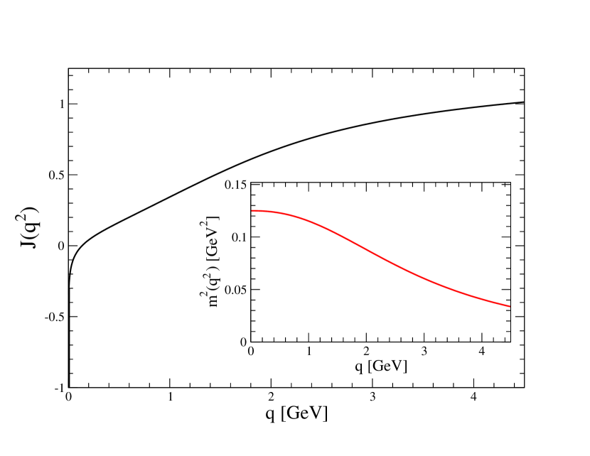
Figure 2: Gluon kinetic term, $J(q^{2})$, and gluon mass, $m^{2}(q^{2})$ (inset). When combined according to Eq. (18), they reproduce accurately the lattice data of [30] for $\Delta(q^{2})$.

Finally, putting together all ingredients described above, we obtain from Eqs. (27) and (28) the SDE-derived result for the $X_{i}$ in the two kinematic configurations of interest. In particular, in the asymmetric limit we obtain the $X_{1}(q^{2},q^{2},0)$ and $q^{2}X_{3}(q^{2},q^{2},0)$ shown in Fig. 3.

As will become apparent in the next section, $X_{1}$ diverges logarithmically, inheriting directly from Eqs. (27) and (28) the corresponding logarithmic divergence of the $J(q^{2})$, given by Eq. (29). Instead, while $X_{3}$ is dominated by the divergent $J^{\prime}(q^{2})$, the combinations $s^{2}X_{3}(s^{2})$ and $q^{2}X_{3}(q^{2},q^{2},0)$ appearing in Eqs. (22) and (23) saturate to finite constants in the infrared.

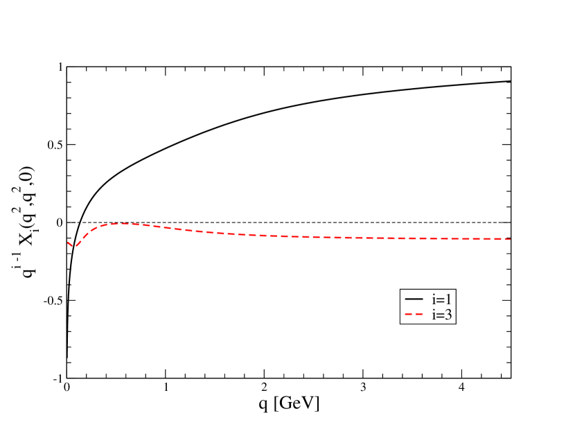
Figure 3: The form factor $X_{1}(q^{2},q^{2},0)$ (black continuous) which composes the tree-level tensor structure of the full three-gluon vertex and the dimensionless combination $q^{2}X_{3}(q^{2},q^{2},0)$ (red dashed).

4 Presentation and analysis of the results

The lattice evaluation of the form factors $\overline{\Gamma}_{1,2}^{\rm sym}$ and $\overline{\Gamma}_{3}^{\rm asym}$ proceeds through the direct simulation of the projections $T_{i}$ and of the gluon propagator $\Delta$ [Eqs. (8), (13) and (4)], and subsequent use of Eqs. (16) and (17), respectively. This is accomplished by exploiting lattice gauge field configurations obtained from simulations with the Wilson action on a 48⁴ lattice at $\beta$=5.8 (970 configurations) and 5.6 (980 configurations), and on a $52^{4}$ lattice at $\beta$=5.6 (980 configurations); for further details see [66]. In addition, we have reanalyzed 1050 gauge-field configurations produced with the tree-level Symanzik action in a $64^{4}$ lattice [16, 19], making thereby apparent that different discretizations of the QCD action provide practically the same results for the three-gluon form factors. In the case of $\overline{\Gamma}_{1}^{\rm sym}$, for the sake of both comparison and implementation of the renormalization condition at $\mu$=4.3 GeV, we have also used earlier results [19], which cover a wider range of momenta. All these configurations have been obtained from large-volume, quenched lattice simulations, neglecting thus the effect of dynamical quarks. The implications of this approximation has been recently assessed in [21], where only minor quantitative but no qualitative effects have been detected.

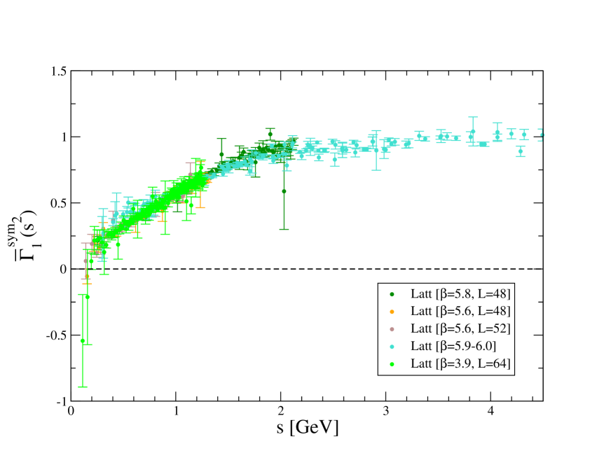
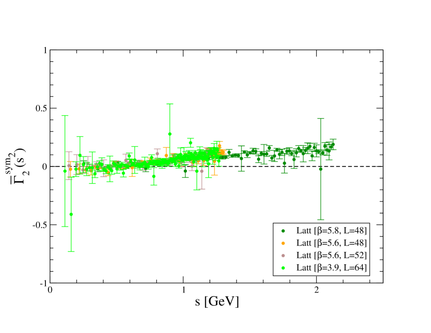
Figure 4: Results for $\overline{\Gamma}_{1}^{\rm sym}(s^{2})$ (upper panel) and $\overline{\Gamma}_{2}^{\rm sym}(s^{2})$ (lower) obtained from three simulations with the Wilson action in a $48^{4}$ lattice at $\beta$=5.8 (dark green) and $\beta$=5.6 (orange), and a $52^{4}$ lattice at $\beta$=5.6 (brown); and from a fourth simulation with the tree-level Symanzik action in a $64^{4}$ lattice at $\beta$=3.9 (light green). Data for $\overline{\Gamma}_{1}^{\rm sym}$ covering a range of larger momenta (turquoise), obtained from several $\beta$’s and volumes and previously published in [67, 68], have been also used to fix the subtraction point at $\mu$=4.3 GeV.

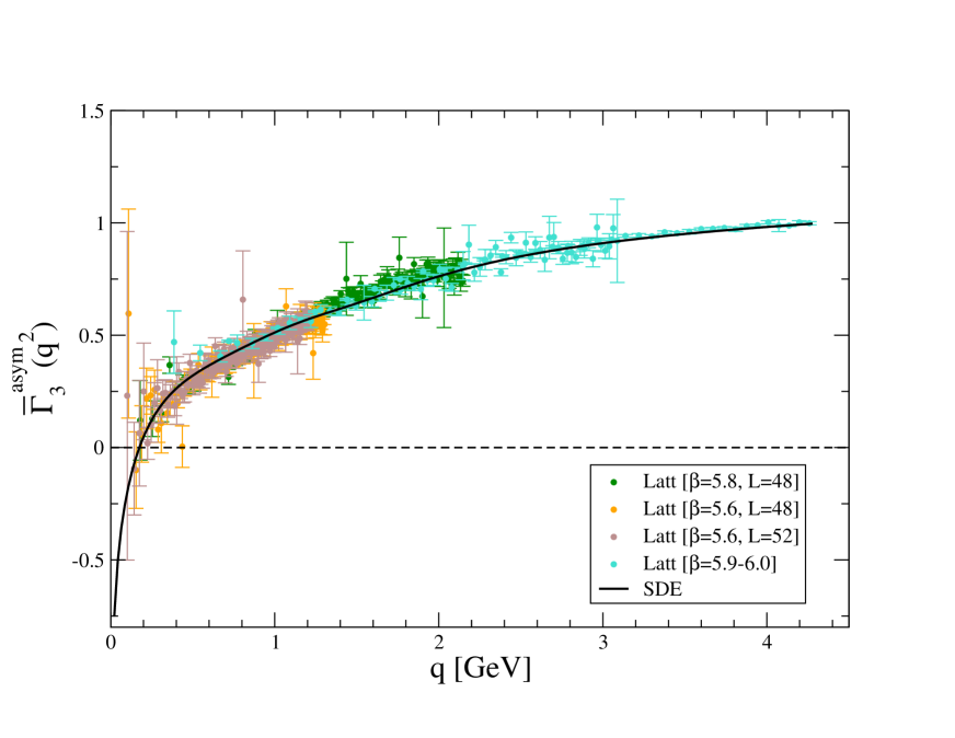
Figure 5: Results for $\overline{\Gamma}_{3}^{\rm asym}(q^{2})$ obtained from the same lattice simulations with the Wilson action quoted in the caption of Fig.  4 (same color code). The black solid line corresponds to the SDE-based computation which, in the asymmetric limit, determines entirely the transversally projected three-gluon vertex.

The new lattice results are shown in Figs. 4 and 5. It should be stressed that the results for $\overline{\Gamma}_{1}^{\rm sym}$ and $\overline{\Gamma}_{3}^{\rm asym}$ are considerably improved with respect to previous analyses [16, 19], capitalizing on a better statistical sample and the careful treatment of discretization artifacts, especially for propagators [66]. In addition, to the best of our knowledge, results for the form factor $\overline{\Gamma}_{2}^{\rm sym}$ are presented for the first time in this letter.

As a very apparent and distinctive feature, $\overline{\Gamma}_{1}^{\rm sym}$ and $\overline{\Gamma}_{3}^{\rm asym}$ clearly display the infrared suppression previously reported [16, 19, 21], accompanied by the characteristic logarithmic divergence near the origin. Instead, $\overline{\Gamma}_{2}^{\rm sym}$ appears to saturate at a small negative constant at low momenta. As we explain below, these behaviors are well understood within the context of the SDE analysis of the previous section.

Quite interestingly, the transverse form factors $Y_{i}$ of the full vertex do not contribute to the projection $\overline{\Gamma}_{3}^{\rm asym}(q^{2})$ in the asymmetric limit, which is thus completely determined through Eq. (23) by $X_{1}(q^{2},q^{2},0)$ and $X_{3}(q^{2},q^{2},0)$. Substituting in it the results of Fig. 3, we obtain the SDE based prediction for $\overline{\Gamma}_{3}^{\rm asym}(q^{2})$, given by the black continuous curve in Fig. 5; evidently, the coincidence with the lattice data is rather notable. This fine agreement may be ultimately attributed to the accurate determination of $J(q^{2})$ over the full range of momenta, following the considerations outlined in section 3.

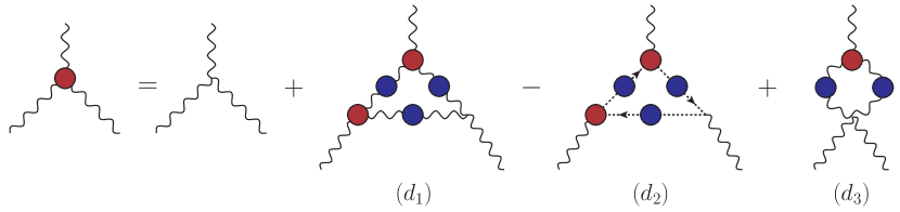
Figure 6: The SDE of the three-gluon vertex at the one-loop dressed level. Blue (red) circles indicate fully dressed propagators (vertices).

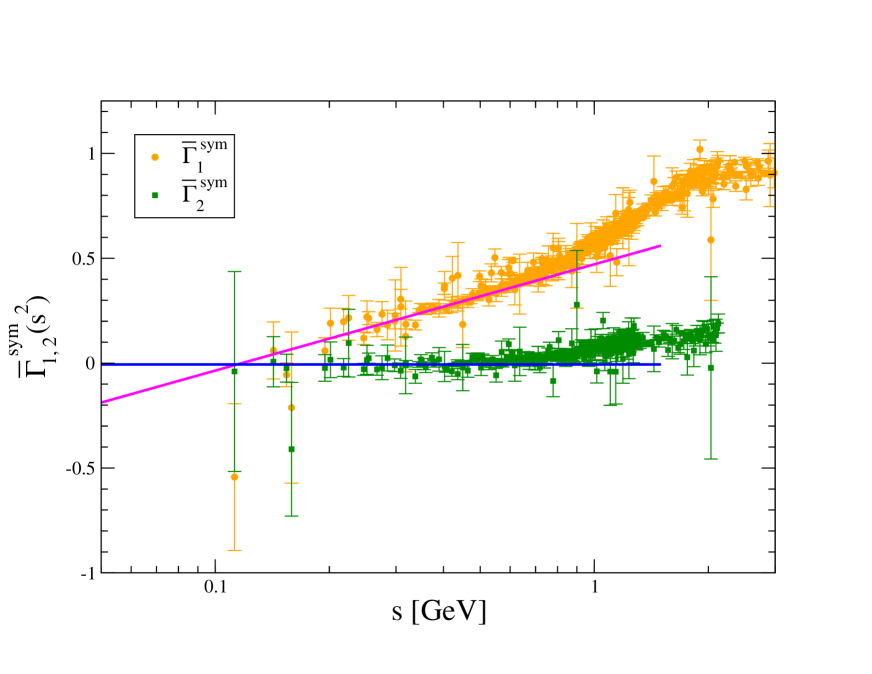
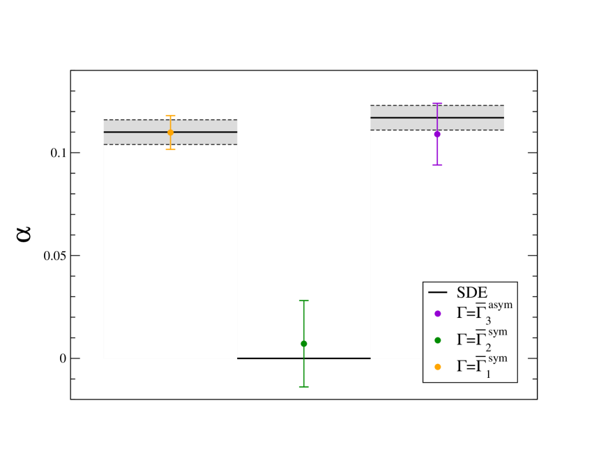
Figure 7: [upper panel]  $\overline{\Gamma}_{1}^{\rm sym}(s^{2})$ (orange) and $\overline{\Gamma}_{2}^{\rm sym}(q^{2})$ (green) plotted in terms of the momentum in logarithmic scale. The solid magenta and blue lines show the asymptotic infrared behavior for the two form factors according, respectively, to Eqs. (32) and (33), the former supplemented by an intercept fitted as explained in the text. [lower panel] The logarithmic derivatives of $\overline{\Gamma}_{1,2}^{\rm sym}(s^{2})$ and $\overline{\Gamma}_{3}^{\rm asym}(q^{2})$ computed from the fit of $f(x)=\alpha\ln{x}+\beta$ [$x=q^{2},s^{2}$] to lattice data (solid circles), with errors representing the statistical deviation from these fits, compared to their SDE estimates in Eqs. (32) and (33) (solid lines). The grey bands for $\overline{\Gamma}_{1}^{\rm sym}(s^{2})$ and $\overline{\Gamma}_{3}^{\rm asym}(q^{2})$ display the uncertainty obtained from the SDE value of $a$, by propagating in it a systematic error of 5 %.

We next focus on the features of the $\overline{\Gamma}_{i}$ in the deep infrared, contrasting the common behavior of $\overline{\Gamma}_{1}^{\rm sym}$ and $\overline{\Gamma}_{3}^{\rm asym}$ to that of $\overline{\Gamma}_{2}^{\rm sym}$. The upshot of this comparison is that, while the former quantities display the infrared divergence known from previous studies, the latter saturates at a finite constant.

To that end, we turn to the SDE for the three-gluon vertex, shown in Fig. 6, and study the transverse form factors $Y_{i}$, which are not accessible through the STI-based construction of the previous section. In particular, a detailed analysis in the symmetric limit reveals that, as $s^{2}\to 0$, $Y_{1}(s^{2})\sim c/s^{4}$ and $Y_{4}(s^{2})\sim d/s^{2}$, for constants $c\approx-0.07$ and $d\approx-0.20$, and, consequently, the combinations $s^{4}Y_{1}$ and $s^{2}Y_{4}$ appearing in Eq. (22) approach constant values at the origin.

The approximation of the $Y_{i}(s^{2})$ through the SDE of Fig. 6 proceeds as follows. First, the projectors that extract the scalar form factors $Y_{i}$ from the tensor structure of the full vertex were determined algebraically. Then, it was verified that the diagram $(d_{3})$ and its permutations do not contribute to the $Y_{i}$ as long as the four-gluon vertex entering there is kept at tree level. The ghost-gluon and three-gluon vertices appearing in diagrams $(d_{1})$ and $(d_{2})$ are then approximated by retaining only form factors that possess a nonvanishing tree-level value.

Specifically, for the three-gluon vertex, we keep only the form factors $X_{1}$, $X_{4}$ and $X_{7}$ [see Eq. (21)], whereas the ghost-gluon vertex is approximated to $\Gamma_{\mu}(q,p,r)=q_{\mu}B_{1}(q,p,r)$, where $q$, $r$ and $p$, denote the momenta of the anti-ghost, ghost and gluon, respectively. Furthermore, to simplify the numerical treatment, these form factors are all considered as functions of the single momentum scale, $s^{2}$, and evaluated in their corresponding totally symmetric limits. Finally, for the ghost and gluon propagators we use fits to lattice data, and for the form factors $X_{i}(s^{2})$ and $B_{1}(s^{2})$ we use the results of Refs [20, 63].

Thus, one reaches the conclusion that the only term that furnishes logarithmically divergent contributions to the $\overline{\Gamma}_{i}$ through Eqs. (22) and (23) is $X_{1}$, while all others provide numerical constants, i.e.,

$$X_{1}(s^{2})\;\mbox{\raisebox{-5.16663pt}[0.0pt][6.88889pt]{$\stackrel{{\scriptstyle\simeq}}{{\scriptscriptstyle s^{2}\to 0}}$}}\;Z_{1}^{\rm sym}F(s^{2})J(s^{2})\;\mbox{\raisebox{-5.16663pt}[0.0pt][6.88889pt]{$\stackrel{{\scriptstyle\simeq}}{{\scriptscriptstyle s^{2}\to 0}}$}}\;Z_{1}^{\rm sym}F(0)\left[a\ln(s^{2}/\mu^{2})+b\right]\,,$$

$$s^{2}X_{3}(s^{2})\;\mbox{\raisebox{-5.16663pt}[0.0pt][6.88889pt]{$\stackrel{{\scriptstyle\simeq}}{{\scriptscriptstyle s^{2}\to 0}}$}}\ \;-Z_{1}^{\rm sym}F(s^{2})s^{2}J^{\prime}(s^{2})\;\mbox{\raisebox{-5.16663pt}[0.0pt][6.88889pt]{$\stackrel{{\scriptstyle\simeq}}{{\scriptscriptstyle s^{2}\to 0}}$}}\;-Z_{1}^{\rm sym}F(0)\,a\,,$$

$$s^{4}Y_{1}(s^{2})\;\mbox{\raisebox{-5.16663pt}[0.0pt][6.88889pt]{$\stackrel{{\scriptstyle\simeq}}{{\scriptscriptstyle s^{2}\to 0}}$}}\ \;c\,,\qquad s^{2}Y_{4}(s^{2})\;\mbox{\raisebox{-5.16663pt}[0.0pt][6.88889pt]{$\stackrel{{\scriptstyle\simeq}}{{\scriptscriptstyle s^{2}\to 0}}$}}\ \;d\,,$$ (31)

Then, from Eqs. (22), (23) and (4) follows that the leading infrared contributions of $\overline{\Gamma}_{1}^{\rm sym}(s^{2})$ and $\overline{\Gamma}_{3}^{\rm asym}(q^{2})$ are given by

$$\overline{\Gamma}_{1}^{\rm sym}(s^{2})\;\mbox{\raisebox{-5.16663pt}[0.0pt][6.88889pt]{$\stackrel{{\scriptstyle\simeq}}{{\scriptscriptstyle s^{2}\to 0}}$}}\;Z_{1}^{\rm sym}F(0)\,a\ln(s^{2}/\mu^{2})\approx 0.110(6)\,\ln(s^{2}/\mu^{2})\,,$$ (32)

$$\overline{\Gamma}_{3}^{\rm asym}(q^{2})\;\mbox{\raisebox{-5.16663pt}[0.0pt][6.88889pt]{$\stackrel{{\scriptstyle\simeq}}{{\scriptscriptstyle q^{2}\to 0}}$}}\;Z_{1}^{\rm asym}F(0)\,a\ln(q^{2}/\mu^{2})\approx 0.117(6)\,\ln(q^{2}/\mu^{2})\,.$$

Evidently, both form factors diverge logarithmically to $-\infty$ at the origin, as captured by the corresponding Figs. 4 and 5, respectively.

Instead, in the same limit, $\overline{\Gamma}_{2}^{\rm sym}(s^{2})$ saturates to a negative constant near zero,

$$\overline{\Gamma}_{2}^{\rm sym}(s^{2})\;\mbox{\raisebox{-5.16663pt}[0.0pt][6.88889pt]{$\stackrel{{\scriptstyle\simeq}}{{\scriptscriptstyle s^{2}\to 0}}$}}\;-\frac{3}{4}\left[Z_{1}^{\rm sym}F(0)\,a+\frac{c}{2}+\frac{d}{3}\right]\,\approx\;-0.006(5)\,.$$ (33)

In obtaining the numerical values quoted above, the finite renormalization constants $Z_{1}^{\rm sym}$ and $Z_{1}^{\rm asym}$ were evaluated perturbatively at $\mu$=4.3 GeV, where they amount to 0.85 and 0.90, respectively. Moreover, the standard value $F(0)$=2.8  [63] has been employed (for the same $\mu$). In addition, as mentioned above, $a\approx 0.046$, while the vertex SDE yields $c\approx-0.07$ and $d\approx-0.20$. The errors have been estimated and displayed in Eqs. (32) and (33), for illustrative purposes, through the propagation in them of an uncertainty of 5 % in the determination of $a$, $c$ and $d$. Note that the numerical difference in the logarithmic slopes of $\overline{\Gamma}_{1}^{\rm sym}$ and $\overline{\Gamma}_{3}^{\rm sym}$ in Eq. (32) is entirely due to the difference between $Z_{1}^{\rm sym}$ and $Z_{1}^{\rm asym}$.

The asymptotic behaviors of $\overline{\Gamma}_{1}^{\rm sym}(s^{2})$ and $\overline{\Gamma}_{2}^{\rm sym}(s^{2})$, given in Eqs. (32) and (33), are next compared to the lattice data; the results of this comparison are shown in the upper panel of Fig. 7. Specifically, we introduce the function $f(x)=\alpha\ln x+\beta$, which represents a straight line on a logarithmic plot ($x=s^{2},q^{2}$). Then, in the case of $\overline{\Gamma}_{1}^{\rm sym}(s^{2})$, the slope $\alpha$ is fixed at the value predicted by Eq. (32), namely $\alpha=0.11$, while the value of its intercept $\beta$ (not predicted by our calculation) is adjusted such that one gets the best fit to lattice data below $s$=0.5 GeV; the result of this procedure is the magenta line. For the case of $\overline{\Gamma}_{2}^{\rm sym}(s^{2})$, one simply fixes $\alpha$ and $\beta$ at their theoretical values $\alpha=0$ and $\beta=-0.006$ (no fitting), thus obtaining the blue line.

A second comparison involves the logarithmic slopes of $\overline{\Gamma}_{1,2}^{\rm sym}(s^{2})$ and $\overline{\Gamma}_{3}^{\rm asym}(q^{2})$. In particularly, we now fit the lattice data below 0.5 GeV with $f(x)$, treating both $\alpha$ and $\beta$ as free parameters, determined by a least-squares fit, including statistical errors. The resulting values for $\alpha$, together with the associated errors, are then compared with the theoretical predictions, as shown in the lower panel of Fig. 7. In all cases, the agreement is excellent, indicating a consistent picture from both SDE and lattice computations.

5 Conclusions

In this work we have explored crucial nonperturbative aspects of the quenched three-gluon vertex through the combination of new lattice data obtained from large-volume simulations and a detailed SDE-based analysis within the PT-BFM framework.

To begin with, we have acquired a clearer view of the infrared logarithmic divergences associated with the form factors $\overline{\Gamma}_{1}^{\rm sym}$ and $\overline{\Gamma}_{3}^{\rm asym}$ by reducing considerably the statistical errors of the lattice simulation. Thus, the presence of these characteristic divergences, already identified in earlier studies (see e.g., [16]), is further supported by the present data. In addition, lattice results for the form factor $\overline{\Gamma}_{2}^{\rm sym}$ are reported here for the first time, strongly supporting its finiteness at the origin.

The new lattice results offer an invaluable opportunity to further scrutinize key dynamical mechanisms from new angles and perspectives. In particular, the nonperturbative features of the Landau-gauge two-point sector of QCD, especially the infrared finiteness of the gluon propagator and the ghost dressing function, are instrumental for obtaining infrared divergent $\overline{\Gamma}_{1}^{\rm sym}$ and $\overline{\Gamma}_{3}^{\rm asym}$, and, and the same time, a finite $\overline{\Gamma}_{2}^{\rm sym}$. The observed agreement between lattice and SDE results clearly corroborates the physical picture put forth, and bolsters up the confidence in the predictivity of continuous functional methods in general.

References

- Marciano and Pagels [1978] W. J. Marciano, H. Pagels, Phys. Rept. 36 (1978) 137.
- Ball and Chiu [1980] J. S. Ball, T.-W. Chiu, Phys. Rev. D22 (1980) 2550.
- Davydychev et al. [1996] A. I. Davydychev, P. Osland, O. V. Tarasov, Phys. Rev. D54 (1996) 4087–4113.
- Alkofer et al. [2005] R. Alkofer, C. S. Fischer, F. J. Llanes-Estrada, Phys. Lett. B611 (2005) 279–288.
- Cucchieri et al. [2006] A. Cucchieri, A. Maas, T. Mendes, Phys. Rev. D74 (2006) 014503.
- Cucchieri et al. [2008] A. Cucchieri, A. Maas, T. Mendes, Phys. Rev. D77 (2008) 094510.
- Huber et al. [2012] M. Q. Huber, A. Maas, L. von Smekal, JHEP 11 (2012) 035.
- Pelaez et al. [2013] M. Pelaez, M. Tissier, N. Wschebor, Phys. Rev. D88 (2013) 125003.
- Aguilar et al. [2014] A. C. Aguilar, D. Binosi, D. Ibañez, J. Papavassiliou, Phys. Rev. D89 (2014) 085008.
- Blum et al. [2014] A. Blum, M. Q. Huber, M. Mitter, L. von Smekal, Phys. Rev. D89 (2014) 061703.
- Eichmann et al. [2014] G. Eichmann, R. Williams, R. Alkofer, M. Vujinovic, Phys. Rev. D89 (2014) 105014.
- Mitter et al. [2015] M. Mitter, J. M. Pawlowski, N. Strodthoff, Phys. Rev. D91 (2015) 054035.
- Williams et al. [2016] R. Williams, C. S. Fischer, W. Heupel, Phys. Rev. D93 (2016) 034026.
- Blum et al. [2015] A. L. Blum, R. Alkofer, M. Q. Huber, A. Windisch, Acta Phys. Polon. Supp. 8 (2015) 321.
- Cyrol et al. [2016] A. K. Cyrol, L. Fister, M. Mitter, J. M. Pawlowski, N. Strodthoff, Phys. Rev. D94 (2016) 054005.
- Athenodorou et al. [2016] A. Athenodorou, D. Binosi, P. Boucaud, F. De Soto, J. Papavassiliou, J. Rodriguez-Quintero, S. Zafeiropoulos, Phys. Lett. B761 (2016) 444–449.
- Duarte et al. [2016] A. G. Duarte, O. Oliveira, P. J. Silva, Phys. Rev. D94 (2016) 074502.
- Corell et al. [2018] L. Corell, A. K. Cyrol, M. Mitter, J. M. Pawlowski, N. Strodthoff, SciPost Phys. 5 (2018) 066.
- Boucaud et al. [2017] P. Boucaud, F. De Soto, J. Rodríguez-Quintero, S. Zafeiropoulos, Phys. Rev. D95 (2017) 114503.
- Aguilar et al. [2019] A. C. Aguilar, M. N. Ferreira, C. T. Figueiredo, J. Papavassiliou, Phys. Rev. D99 (2019) 094010.
- Aguilar et al. [2020] A. C. Aguilar, F. De Soto, M. N. Ferreira, J. Papavassiliou, J. Rodríguez-Quintero, S. Zafeiropoulos, Eur. Phys. J. C 80 (2020) 154.
- Aguilar et al. [2019] A. C. Aguilar, M. N. Ferreira, C. T. Figueiredo, J. Papavassiliou, Phys. Rev. D 100 (2019) 094039.
- Vujinovic and Mendes [2019] M. Vujinovic, T. Mendes, Phys. Rev. D99 (2019) 034501.
- Cornwall [1982] J. M. Cornwall, Phys. Rev. D26 (1982) 1453.
- Bernard [1983] C. W. Bernard, Nucl. Phys. B219 (1983) 341.
- Donoghue [1984] J. F. Donoghue, Phys. Rev. D29 (1984) 2559.
- Wilson et al. [1994] K. G. Wilson, T. S. Walhout, A. Harindranath, W.-M. Zhang, R. J. Perry, S. D. Glazek, Phys. Rev. D49 (1994) 6720–6766.
- Philipsen [2002] O. Philipsen, Nucl. Phys. B628 (2002) 167–192.
- Cucchieri and Mendes [2007] A. Cucchieri, T. Mendes, PoS LAT2007 (2007) 297.
- Bogolubsky et al. [2007] I. L. Bogolubsky, E. M. Ilgenfritz, M. Muller-Preussker, A. Sternbeck, PoS LATTICE2007 (2007) 290.
- Bogolubsky et al. [2009] I. Bogolubsky, E. Ilgenfritz, M. Muller-Preussker, A. Sternbeck, Phys. Lett. B676 (2009) 69–73.
- Oliveira and Silva [2009] O. Oliveira, P. Silva, PoS LAT2009 (2009) 226.
- Ayala et al. [2012] A. Ayala, A. Bashir, D. Binosi, M. Cristoforetti, J. Rodriguez-Quintero, Phys. Rev. D86 (2012) 074512.
- Aguilar and Natale [2004] A. C. Aguilar, A. A. Natale, JHEP 08 (2004) 057.
- Aguilar and Papavassiliou [2006] A. C. Aguilar, J. Papavassiliou, JHEP 12 (2006) 012.
- Aguilar et al. [2008] A. C. Aguilar, D. Binosi, J. Papavassiliou, Phys. Rev. D78 (2008) 025010.
- Boucaud et al. [2008] P. Boucaud, J. Leroy, L. Y. A., J. Micheli, O. Pène, J. Rodríguez-Quintero, JHEP 06 (2008) 099.
- Fischer et al. [2009] C. S. Fischer, A. Maas, J. M. Pawlowski, Annals Phys. 324 (2009) 2408–2437.
- Dudal et al. [2008] D. Dudal, J. A. Gracey, S. P. Sorella, N. Vandersickel, H. Verschelde, Phys. Rev. D78 (2008) 065047.
- Rodriguez-Quintero [2011] J. Rodriguez-Quintero, JHEP 1101 (2011) 105.
- Tissier and Wschebor [2010] M. Tissier, N. Wschebor, Phys. Rev. D82 (2010) 101701.
- Pennington and Wilson [2011] M. Pennington, D. Wilson, Phys. Rev. D84 (2011) 119901.
- Cloet and Roberts [2014] I. C. Cloet, C. D. Roberts, Prog. Part. Nucl. Phys. 77 (2014) 1–69.
- Fister and Pawlowski [2013] L. Fister, J. M. Pawlowski, Phys. Rev. D88 (2013) 045010.
- Cyrol et al. [2015] A. K. Cyrol, M. Q. Huber, L. von Smekal, Eur. Phys. J. C75 (2015) 102.
- Binosi et al. [2015] D. Binosi, L. Chang, J. Papavassiliou, C. D. Roberts, Phys. Lett. B742 (2015) 183–188.
- Cyrol et al. [2018] A. K. Cyrol, J. M. Pawlowski, A. Rothkopf, N. Wink, SciPost Phys. 5 (2018) 065.
- Alkofer and von Smekal [2001] R. Alkofer, L. von Smekal, Phys. Rept. 353 (2001) 281.
- Fischer [2006] C. S. Fischer, J. Phys. G32 (2006) R253–R291.
- Boucaud et al. [2008] P. Boucaud, J.-P. Leroy, A. L. Yaouanc, J. Micheli, O. Pene, et al., JHEP 0806 (2008) 012.
- Cornwall and Papavassiliou [1989] J. M. Cornwall, J. Papavassiliou, Phys. Rev. D40 (1989) 3474.
- Pilaftsis [1997] A. Pilaftsis, Nucl. Phys. B487 (1997) 467–491.
- Binosi and Papavassiliou [2009] D. Binosi, J. Papavassiliou, Phys. Rept. 479 (2009) 1–152.
- Abbott [1981] L. F. Abbott, Nucl. Phys. B185 (1981) 189.
- Binosi and Papavassiliou [2008] D. Binosi, J. Papavassiliou, Phys. Rev. D77 (2008) 061702.
- Gracey et al. [2019] J. A. Gracey, H. Kißler, D. Kreimer, Phys. Rev. D 100 (2019) 085001.
- Alles et al. [1997] B. Alles, D. Henty, H. Panagopoulos, C. Parrinello, C. Pittori, D. G. Richards, Nucl. Phys. B 502 (1997) 325–342.
- Boucaud et al. [1998a] P. Boucaud, J. P. Leroy, J. Micheli, O. Pene, C. Roiesnel, JHEP 10 (1998a) 017.
- Boucaud et al. [1998b] P. Boucaud, J. P. Leroy, J. Micheli, O. Pene, C. Roiesnel, JHEP 12 (1998b) 004.
- Hasenfratz and Hasenfratz [1980] A. Hasenfratz, P. Hasenfratz, Phys. Lett. B 63 (1980) 165.
- Davydychev et al. [1998] A. I. Davydychev, P. Osland, O. V. Tarasov, Phys. Rev. D58 (1998) 036007.
- Binosi et al. [2012] D. Binosi, D. Ibañez, J. Papavassiliou, Phys. Rev. D86 (2012) 085033.
- Aguilar et al. [2019] A. C. Aguilar, M. N. Ferreira, C. T. Figueiredo, J. Papavassiliou, Phys. Rev. D99 (2019) 034026.
- Aguilar et al. [2012] A. C. Aguilar, D. Ibanez, V. Mathieu, J. Papavassiliou, Phys. Rev. D85 (2012) 014018.
- Aguilar et al. [2020] A. C. Aguilar, M. N. Ferreira, J. Papavassiliou, Eur. Phys. J. C 80 (2020) 887.
- Boucaud et al. [2018] P. Boucaud, F. De Soto, K. Raya, J. Rodríguez-Quintero, S. Zafeiropoulos, Phys. Rev. D98 (2018) 114515.
- Boucaud et al. [2003] P. Boucaud, F. De Soto, A. Le Yaouanc, J. P. Leroy, J. Micheli, H. Moutarde, O. Pene, J. Rodriguez-Quintero, JHEP 04 (2003) 005.
- Boucaud et al. [2004] P. Boucaud, F. De Soto, A. Le Yaouanc, J. P. Leroy, J. Micheli, O. Pene, J. Rodriguez-Quintero, Phys. Rev. D 70 (2004) 114503.