Hi constraints from the cross-correlation of eBOSS galaxies and Green Bank Telescope intensity maps

Abstract

We present the joint analysis of Neutral Hydrogen (Hi) Intensity Mapping observations with three galaxy samples: the Luminous Red Galaxy (LRG) and Emission Line Galaxy (ELG) samples from the eBOSS survey, and the WiggleZ Dark Energy Survey sample. The Hi intensity maps are Green Bank Telescope observations of the redshifted $21\rm cm$ emission on $100\,{\rm deg}^{2}$ covering the redshift range $0.6<z<1.0$. We process the data by separating and removing the foregrounds present in the radio frequencies with FastICA. We verify the quality of the foreground separation with mock realisations, and construct a transfer function to correct for the effects of foreground removal on the Hi signal. We cross-correlate the cleaned Hi data with the galaxy samples and study the overall amplitude as well as the scale-dependence of the power spectrum. We also qualitatively compare our findings with the predictions by a semi-analytic galaxy evolution simulation. The cross-correlations constrain the quantity $\Omega_{\textrm{H{i}}}b_{\textrm{H{i}}}r_{\textrm{H{i}},{\rm opt}}$ at an effective scale $k_{\rm eff}$, where $\Omega_{\textrm{H{i}}}$ is the Hi density fraction, $b_{\textrm{H{i}}}$ is the Hi bias, and $r_{\textrm{H{i}},{\rm opt}}$ the galaxy-hydrogen correlation coefficient, which is dependent on the Hi content of the optical galaxy sample. At $k_{\rm eff}=0.31\,h/{\rm Mpc}$ we find $\Omega_{\textrm{H{i}}}b_{\textrm{H{i}}}r_{\textrm{H{i}},{\rm Wig}}=[0.58\pm 0.09\,{\rm(stat)\pm 0.05\,{\rm(sys)}}]\times 10^{-3}$ for GBT-WiggleZ, $\Omega_{\textrm{H{i}}}b_{\textrm{H{i}}}r_{\textrm{H{i}},{\rm ELG}}=[0.40\pm 0.09\,{\rm(stat)\pm 0.04\,{\rm(sys)}}]\times 10^{-3}$ for GBT-ELG, and $\Omega_{\textrm{H{i}}}b_{\textrm{H{i}}}r_{\textrm{H{i}},{\rm LRG}}=[0.35\pm 0.08\,{\rm(stat)\pm 0.03\,{\rm(sys)}}]\times 10^{-3}$ for GBT-LRG, at $z\simeq 0.8$. We also report results at $k_{\rm eff}=0.24\,h/{\rm Mpc}$ and $k_{\rm eff}=0.48\,h/{\rm Mpc}$. With little information on Hi parameters beyond our local Universe, these are amongst the most precise constraints on neutral hydrogen density fluctuations in an underexplored redshift range.

1 Introduction

The redshifted 21cm emission from Neutral Hydrogen (Hi) gas provides an alternative view into the structure, dynamics, and evolution of galaxies. Hi gas is the fundamental fuel for molecular gas and star formation and plays an essential role in galaxy formation and evolution and models thereof. Blind Hi surveys of the local Universe provide constraints on the Hi abundance via the Hi mass function (Jones et al., 2020; Zwaan et al., 2003) and the global Hi abundance $\Omega_{\textrm{H{i}}}=(4.3\pm 0.3)10^{-4}H_{0}/70$ (Martin et al., 2010). Spectral stacking techniques have also been used (see e.g. Hu et al. 2019 and references therein).

Targeted deep surveys investigate the Hi scaling relations with galaxy properties such as stellar mass, star formation activity, or star formation efficiency with multi-wavelength data. It has been inferred that cold gas properties are tightly related to their star-forming properties and less to their morphology, with scatter on the relations being driven by inflows mechanisms and dynamics (Cook et al., 2019; Chen et al., 2019). Hi gas mass has been found to strongly anti-correlate with stellar mass, particularly when traced by NUV-r colour (Catinella et al., 2018). Multiple studies on the Hi deficiency in high density regions such as the VIRGO cluster confirm the high impact of environment on atomic gas abundance (see Cortese et al. 2011; Dénes et al. 2014; Reynolds et al. 2020). Bok et al. (2020) studied environmental effects using an infra-red selected sample of Hi detections finding a reduced scatter in scaling relations for isolated galaxies. Some investigations have been made into the relation between Hi and its host halo mass to constrain a Hi halo occupation distribution, see for example Guo et al. (2020) or Paul et al. (2017). The most important limitations of all blind and targeted Hi surveys are their sensitivity limitations on relatively Hi-rich galaxy samples, as well as volume-limited sample sizes. Additionally, there is little information on Hi abundances and scaling relations beyond our local Universe (Crighton et al., 2015; Padmanabhan et al., 2016; Hu et al., 2019).

The technique of Hi intensity mapping has been proposed to perform fast observations of very large cosmic volumes in a wide redshift range. Intensity mapping does not rely on detecting individual galaxies, but instead measures the integrated redshifted spectral line emission without sensitivity cuts in large voxels on the sky, whith the voxel volume determined by the radio telescope beam and frequency channelisation, see e.g. (Battye et al., 2004; Chang et al., 2008; Wyithe & Loeb, 2009; Mao et al., 2008; Peterson et al., 2009; Chang et al., 2010; Seo et al., 2010; Ansari et al., 2012). Using the Hi signal as a biased tracer for the underlying matter distribution, it is possible to probe the large-scale structure of the Universe, and constrain both, global Hi properties and cosmological parameters. Particularly, the amplitude of the Hi intensity mapping clustering signal scales with the global Hi energy density $\Omega_{\rm HI}$ and can constrain it for various redshifts.

The next few years will see data from a number of Hi intensity mapping experiments, for example the proposed MeerKLASS survey at the Square Kilometre Array (SKA) precursor MeerKAT (Santos et al., 2017; Wang et al., 2021), an Hi survey at the 500m dish telescope FAST (Hu et al., 2020), and multiple surveys with the SKA using the single-dish mode of operation (Battye et al., 2013; Bull et al., 2015; Santos et al., 2017; SKA Cosmology SWG et al., 2020). Other international experiments include the CHIME project (Bandura et al., 2014), HIRAX (Newburgh et al., 2016), and Tianlai (Li et al., 2020b; Wu et al., 2021).

The observed intensity maps suffer from foreground contamination from Galactic and extra-galactic sources. Our own Galaxy emits high synchroton and free-free emission up to three orders of magnitude brighter than the redshifted 21cm line (Matteo et al., 2002), which need to be subtracted from the data (see e.g. Wolz et al. 2014; Alonso et al. 2015; Shaw et al. 2015; Olivari et al. 2015; Cunnington et al. 2019; Carucci et al. 2020). To-date, the intensity mapping signal has not been detected in auto-correlation due to calibration errors, radio frequency interference, residual foregrounds and noise systematics (Switzer et al., 2013, 2015; Harper et al., 2018; Li et al., 2020a). The impact of the contaminations can be reduced by cross-correlating the Hi signal with optical surveys. The first successful detection with Green Bank Telescope (GBT) data has been achieved at $0.6<z<1.0$ using the cross-correlations with the DEEP2 survey (Chang et al., 2010), followed by the cross-correlations with the WiggleZ Dark Energy survey (Masui et al., 2013). The GBT-WiggleZ correlations at $z=0.8$ have constrained the combination of the Hi abundance $\Omega_{\textrm{H{i}}}$ and linear Hi bias $b_{\textrm{H{i}}}$, finding $\Omega_{\textrm{H{i}}}b_{\textrm{H{i}}}r_{\textrm{H{i}},{\rm Wig}}=[4.3\pm 1.1]\times 10^{-4}$, where $r_{\textrm{H{i}},{\rm Wig}}$ is the galaxy-Hi cross-correlation coefficient. The significance of detection was $7.4\sigma$ for the combined 1hr and 15hr fields observations (Masui et al., 2013).

More recently, the Parkes radio telescope reported a cross-correlation detection at $z\simeq 0.1$ using galaxies from the 2dF survey (Anderson et al., 2018). In this study, upon dividing the galaxies into red and blue colours, a drop in amplitude on small scales was detected for the red sample. This result is in agreement with aforementioned studies on Hi in dense environments as well as with theoretical predictions on the Hi -galaxy cross-correlation of a correlation coefficient dependent on the Hi content of the optical galaxy sample (Wolz et al., 2016a). Additionally, it is also predicted that the amplitude of the shot noise on the cross-power spectra scales with the averaged Hi mass of the galaxy sample (Wolz et al., 2017).

In this work, we present the analysis of the extended and deepened 1-hr field observations from the previous study in Masui et al. (2013). We apply the foreground subtraction technique FastICA as outlined in Wolz et al. (2016b) and, for the first time, construct the FastICA transfer function using mock lognormal simulations. We cross-correlate the Hi intensity mapping data with three distinct galaxy samples, the Emission Line Galaxy (ELG) and Luminous Red Galaxy (LRG) samples from the eBOSS survey (Raichoor et al., 2020; Ross et al., 2020; Alam et al., 2021) as well as the previously considered WiggleZ survey (Blake et al., 2011). This leads to a robust confirmation of detection with multiple galaxy samples, as well as a first attempt to quantify the cross-correlation coefficient between Hi and the galaxy sample properties. We also qualitatively compare our measurements with predictions from the semi-analytic galaxy evolution model DARK SAGE (Stevens et al., 2016) to investigate the Hi contents of the samples. Finally, we use the cross-correlation measurements to constrain the quantity $\Omega_{\textrm{H{i}}}b_{\textrm{H{i}}}r_{\textrm{H{i}},{\rm opt}}$, and also provide estimates for $\Omega_{\textrm{H{i}}}$ using external estimates for $b_{\textrm{H{i}}}$ and $r_{\textrm{H{i}},{\rm opt}}$.

The paper is organised as follows: In Section 2, we describe the GBT intensity maps, and the WiggleZ and eBOSS galaxy samples. We also give a brief description of our simulations. In Section 3, we outline the application of the FastICA technique to the GBT maps, as well as the construction of the foreground transfer function. In Section 4 we present and discuss our cross-correlation results. In Section 5 we derive the Hi constraints. We conclude in Section 6. The appendix contains details on our mock galaxy selection in Appendix A as well as figures of our covariance analysis in Appendix B.

2 Description of data products

2.1 Green Bank Telescope intensity maps

The Hi intensity mapping data from the Green Bank Telescope (GBT) used in this study is located in the 1hr field of the WiggleZ Dark Energy survey at right ascension $5.43\degree<{\rm RA}<18.9\degree$ and declination $-2.55\degree<{\rm DEC}<4.8\degree$. This field was observed with the receiver band at $700<\nu<900\,\rm{MHz}$, which results in a 21cm redshift range of $0.6<z<1.0$. The data is divided into $N_{\nu}=256$ frequency channels with width $\delta\nu=0.78\,\rm MHz$, after rebinning from the original 2048 correlator channels. The observational spatial resolution of the maps, quantified by the full width half maximum (FWHM) of the GBT telescope beam, evolves from $\rm{FWHM}\approx 0.31\deg$ at $\nu=700\,\rm{MHz}$ to $\rm{FWHM}\approx 0.25\deg$ at $\nu=900\,\rm{MHz}$. The maps are pixelised with spatial resolution angle of $\delta\theta\approx\delta\phi=0.067\deg$, which results in $N_{\rm RA}=217$ pixels in right ascension and $N_{\rm DEC}=119$ pixels in declination. The pixel size was chosen such that approximately 4 pixels cover the beam at mid-frequency $\nu\approx 800\,\rm MHz$, and the instrumental noise can be approximated as uncorrelated between pixels. The maps are an extended version of the previously published observations described in Masui et al. (2013) with added scans to increase the area to $100\deg^{2}$ and survey depth to $100\,\rm hrs$ total integration time collected from 2010-2015. The details on Radio Frequency Interference (RFI) flagging, calibration, and map making procedures can be found in Masui et al. (2013); Switzer et al. (2013); Masui (2013).

As described in previous studies, the GBT intensity maps suffer a number of instrumental systematic effects. To reduce the impact of the systematic effects, the following measures have been taken:

• RFI and resonance: The data is contaminated by RFI and two telescope resonance frequencies. Figure 1 shows the mean absolute temperature of each channel as a function of redshift. The red line shows the initial data with strong RFI contamination at the lowest redshift as well as towards the highest redshift end. The RFI flagging causes an overall signal loss of $\approx 11\%$, more details on the RFI flagging process can be found in (Switzer et al., 2013). The two telescope resonances can be seen at $\nu=798\,\rm MHz$ and $\nu=817\,\rm MHz$ which corresponds to the dips in amplitude seen at $z=0.78$ and $z=0.74$. To minimise these effects, we dismiss the lowest 30 channels in redshift and the intervals around the resonances before the foreground removal.

• Sub-seasons: The time-ordered data is divided into 4 seasons $\rm\{A,B,C,D\}$. Thermal noise is uncorrelated between these seasons, which have been chosen to have similar integration depth and coverage (Switzer et al., 2013). More specifically, the Gaussian sampling noise and time-dependent RFI in each season are independent, however, observational systematics in seasons can correlate. The individual season data is shown as faded purple and yellow lines in Figure 1.

• Masking: The noise properties are highly anisotropic towards the spatial edges of the map due to the scanning strategy and resulting anisotropic survey depth. We therefore mask out 15 pixels per side, which significantly reduces residual anisotropic noise in the foreground subtracted maps. About an order of magnitude decrease of the mean temperature of the maps is found comparing the original and masked foreground subtracted data marked by the purple and yellow lines in Figure 1. The solid purple and yellow lines show the signal averaged over the four seasons, and the faded lines around them show the individual seasons.

• Beam: The beam of the instrument can be approximated by a symmetric Gaussian function with a frequency-dependent FWHM with maximum ${\rm FWHM}_{\rm max}\approx 0.31\deg$. In order to aid the data analysis as well as to minimise systematics caused by polarisation leakage of the receiver (Switzer et al., 2013), we convolve the data to a common Gaussian beam with ${\rm FWHM}=1.4\,{\rm FWHM_{max}}$, which results in an angular resolution of ${\rm FWHM}=0.44\deg$. This strategy is adopted as polarization leakage is considered the most significant contaminant in the data. However, we acknowledge that this would not be an optimal strategy to mitigate effects of beam chromaticity, as shown in Spinelli et al. (2021).

Figure 1 shows that even after applying these measures and removing foregrounds modelled by 36 Independent Components, the mean temperature of the Hi maps is about an order of magnitude higher than the theoretically predicted Hi brightness temperature. We model this following Chang et al. (2010) and Masui et al. (2013) as:

$$T_{\rm HI}(z)=0.29\frac{\Omega_{\rm HI}}{10^{-3}}\left(\frac{\Omega_{m}+\Omega_{\Lambda}(1+z)^{-3}}{0.37}\right)^{-0.5}\left(\frac{1+z}{1.8}\right)^{0.5}{\rm mK}\,$$ (1)

which is shown as the green dotted line. We are unable to directly detect the Hi signal with our current pipeline in this systematics dominated data.

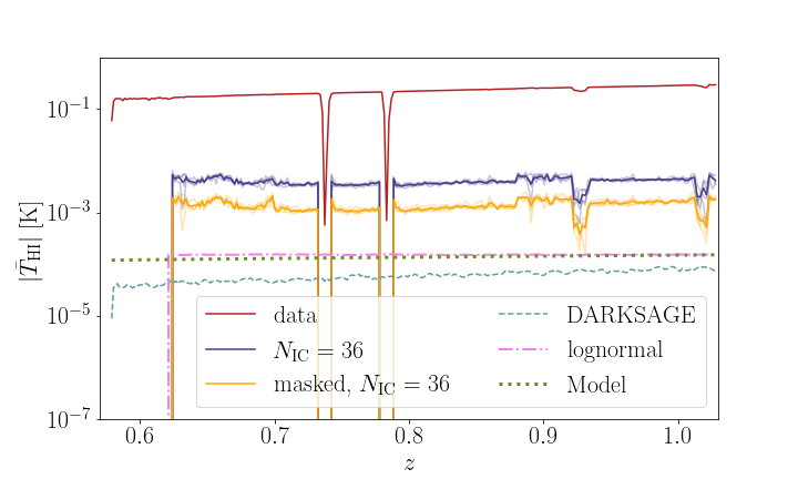
Figure 1: Mean of the absolute temperature of the GBT intensity maps as a function of redshift, binned into 256 frequency channels. The solid lines represent the mean over the 4 GBT seasons with original data (red), the FastICA foreground subtracted data with $N_{\rm IC}=36$ (purple), and the masked, FastICA foreground subtracted data with $N_{\rm IC}=36$ (yellow). The faded purple and yellow lines indicate the individual seasons. The green dotted line represents the analytical brightness temperature prediction from Equation 1, the pink dashed line the averaged temperature of the lognormal simulations used for the foreground removal transfer function (see Section 3 for details), and the teal dashed line the numerical prediction from the DARK SAGE simulation described in Section 2.

2.2 Galaxy samples

In this study, we consider three galaxy samples overlapping with the Hi intensity maps in the 1hr field. We use the WiggleZ Dark Energy Survey galaxy sample based on Blake et al. (2011) as previously presented in Masui et al. (2013). And, for the first time, we use the SDSS Emission Line Galaxy (ELG) and Luminous Red Galaxy (LRG) sample of the eBOSS survey (DR16) for the Hi-galaxy cross-correlation analysis.

In Figure 2, we show the spatial footprint of each survey in the 1hr field, where dark patches indicate unobserved regions and the red lines mark the edge masking as part of the systematics mitigation of the GBT data. The LRG and WiggleZ samples both have a reduced spatial overlap with the GBT data as it has unobserved regions, however, since we introduce the red mask, this effect is somewhat diminished. The ELG sample has the most complete overlap with the GBT data.

WiggleZ - The WiggleZ galaxies are part of the WiggleZ Dark Energy Survey (Drinkwater et al., 2010), a large-scale spectroscopic survey of emission-line galaxies selected from UV and optical imaging. These are active, highly star-forming objects, and it has been suggested that they contain a large amount of Hi gas to fuel their star-formation. The selection function (Blake et al., 2010) has angular dependence determined primarily by the UV selection, and redshift coverage favouring the $z=0.6$ end of the radio band. The galaxies are binned into volumes with the same pixelization as the radio maps and divided by the selection function, and we consider the cross-power with respect to optical over-density.

eBOSS ELG - The extended Baryon Oscillation Spectroscopic Survey (eBOSS; Dawson et al. 2016), is part of the SDSS-IV experiment (Blanton et al., 2017), and has spectroscopically observed $173,736$ ELGs in the redshift range $0.6<z<1.1$ (Raichoor et al., 2020). Targets were colour-selected from the DECaLS photometric survey, with an algorithm designed to select OII emitting galaxies with high star-formation rates. Spectra were then obtained using the BOSS spectrographs (Smee et al., 2013) mounted on the 2.5-meter Sloan telescope (Gunn et al., 2006). Details of the sample, including standard Baryon Acoustic Oscillation (BAO) and Redshift Space Distortion (RSD) measurements can be found in Raichoor et al. (2020); Tamone et al. (2020); de Mattia et al. (2021).

eBOSS LRG - Luminous Red Galaxies were observed by eBOSS from a target sample selected (Prakash et al., 2015) from SDSS DR13 photometric data (Albareti et al., 2017), combined with infrared observations from the WISE satellite (Lang et al., 2016). This sample was selected to be composed of large, old, strongly-biased galaxies, typically found in high mass haloes. In total, the sample contains $174,816$ LRGs with measured redshifts between $0.6<z<1.0$. In our analysis we do not combine the eBOSS LRGs with the $z>0.6$ BOSS CMASS galaxies as in the standard BAO and RSD measurements (Bautista et al., 2020; Gil-Marin et al., 2020). Possible systematics related to the eBOSS LRG sample have been quantified via realistic N-body-based mocks in (Rossi et al., 2021). The cosmological interpretation of the BAO and RSD results from all eBOSS samples was presented in Alam et al. (2021).

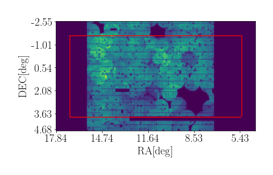
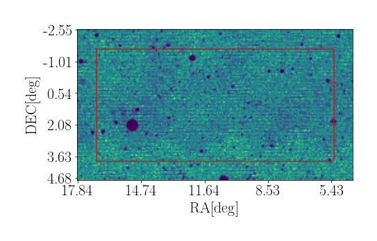
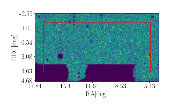
Figure 2: Spatial footprint of the galaxy samples. From top to bottom: WiggleZ, ELG, and LRG samples. The survey window is binned on the same spatial pixelisation as the GBT data with pixel size of $\delta\theta=\delta\phi=0.067\deg$.

Figure 3 shows the galaxy density distribution with redshift, $N(z)$, where we binned the data according to the frequency bins of the GBT intensity mapping data. This implies that the bin size is constant in frequency rather than redshift, and the co-moving volume of the bins evolves with redshift. The line-of-sight resolution is very high with an average redshift bin size of $\delta z\approx 0.0016$. The galaxy density normalisation has taken into account the evolving co-moving volume of the bins.

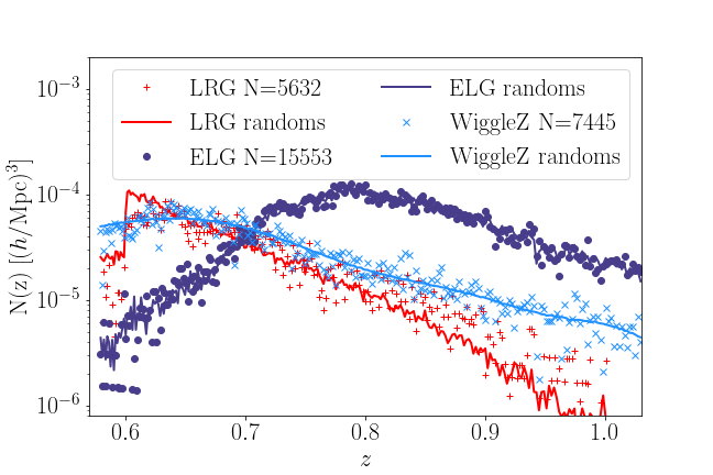
Figure 3: Galaxy density distribution with redshift. The solid lines represent the mean of the random catalogues used to determine the selection function, and the markers show the data points of the samples.

We can see that both the WiggleZ galaxy and eBOSS LRG samples peak towards the low-redshift end of the data, around $z\sim 0.6$, and that the density of the LRGs drops significantly faster with redshift compared to the other samples. The eBOSS ELG distribution is at higher redshift and peaks around $z\sim 0.8$ with a significant signal density at the highest redshift $z\sim 1.0$. As the low redshift end of the intensity maps is significantly contaminated by RFI, we lose the peak of the LRG and WiggleZ sample in the cross-correlation. The total number of galaxies for the samples is significantly reduced from $N_{\rm Wig,all}=7445$, $N_{\rm LRG,all}=5632$, and $N_{\rm ELG,all}=15553$ to $N_{\rm Wig}=4815$, $N_{\rm LRG}=3281$, and $N_{\rm ELG}=8534$, respectively.

2.3 Simulations

In order to examine the underlying astrophysics of Hi-galaxy cross-correlations, we use the online service “Theoretical Astrophysical Observatory” (TAO) to create a mock galaxy catalogue. We create the galaxy distribution using the semi-analytic galaxy formation model DARK SAGE (Stevens et al., 2016) run on the merger trees of the Millennium simulation (Springel et al., 2006) with box of comoving side length of $500\,{\rm Mpc}/h$. DARK SAGE is a modified version of SAGE (Croton et al., 2006), which includes a pressure-based description of the atomic and molecular gas components of the cold gas based on an advanced computation of disk structure and cooling processes. DARK SAGE is calibrated to reproduce the Stellar, Hi and ${\rm H}_{2}$ Mass Functions as well as the fraction of Hi to stellar mass as a function of stellar mass as observed at $z=0$. For more details, we refer the reader to Stevens et al. (2016). In our study, we create a lightcone with the same survey geometry covering the redshift range $0.6<z<1.0$, and the same spatial and redshift binning as the GBT data.

We post-process the galaxy catalogue from TAO to create Hi intensity maps as well as the three optical galaxy samples. We apply the same resolution-motivated mass cut as in Stevens et al. (2016) and only use galaxies with $M_{*}>10^{8.5}M_{\rm sun}$ for our analysis. This might be a slightly conservative choice compared to, for example, Spinelli et al. (2020), but the specific purpose of this simulation is to examine the Hi content of the galaxy samples rather than the universal properties of the Hi maps. Furthermore, Spinelli et al. (2020) showed that for low redshift observations, resolution effects of Millennium-based simulations are negligible for $k<1h/{\rm Mpc}$.

For the Hi intensity maps, we sum the Hi mass $M_{i,{\rm HI}}$ of all galaxies falling into the same pixel $i$ with spatial dimension $\delta\phi=\delta\theta=0.067\deg$ and the same frequency bins as the data, where we also include redshift space distortions via line-of-sight peculiar velocities of the galaxies. We transform the maps in brightness temperature using

$$T_{\rm HI}(x_{i})=\frac{3A_{12}\hbar c^{3}}{32\pi m_{\rm H}k_{\rm B}\nu_{\rm HI}^{2}}\frac{(1+z_{i})^{2}}{H(z_{i})}\frac{M_{i,\rm HI}}{V_{\rm pix}}\,,$$ (2)

with $\hbar$ the Planck constant, $k_{\rm B}$ the Boltzmann constant, $m_{\rm H}$ the Hydrogen atom mass, $\nu_{\rm HI}$ the rest frequency of the Hi emission line, $c$ the speed of light, $A_{12}$ the transition rate of the spin flip, and $V_{\rm pix}$ the co-moving volume of the pixel at mid-redshift. We also remove the mean temperature $\bar{T}_{\textrm{H{i}}}$ of each map to create temperature fluctuation maps, also referred to as over-temperature maps. We then convolve the resulting maps with a Gaussian beam with ${\rm FWHM}=0.44\deg$.

Based on our galaxy lightcone catalogue, we additionally create optical, near-infrared and UV band emissions for each galaxy with the Spectral Energy Distribution (SED) module of TAO, using the Chabrier Initial Mass Function (Conroy & van Dokkum, 2012). The SED is based on the star-formation history primarily dependent on stellar mass, age, and metallicity of each galaxy. Galaxy photometry is applied after the construction of the SED. In our case, we use the SDSS filter $\{g,r,i,z\}$, and the Galex near ultra-violet filter NUV and FUV, as well as the near-infrared filter IRAC1 as an approximation for the WISE filter W1.

We apply the same observational colour cuts to the simulated lightcone to create mock galaxy samples resembling the eBOSS LRG, eBOSS ELG and WiggleZ selections, following the approach in Wolz et al. (2016a). Details on the target selection are given in Appendix A.

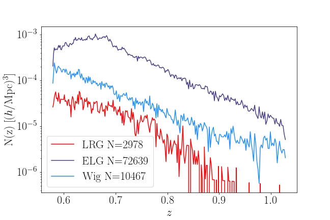
Figure 4: The galaxy density of the mock galaxy samples from the DARK SAGE simulation as a function of redshift.

In Figure 4, we show the redshift distribution of the resulting mock galaxy samples from the semi-analytic simulation. We note that the overall galaxy numbers are off by several factors as there are many observational subtleties that can not be replicated by our approach. In addition, the eBOSS ELG-like sample peaks at slightly lower redshift around $z\sim 0.7$ compared to the actual data. However, we can see that the overall trends of the galaxy redshift distribution are present in our mock samples, and we believe that they qualitatively sample the respective galaxy types and allow us to investigate the relation between galaxy types and their Hi abundance. In this work, we use the simulation to qualitatively study the predicted Hi abundance in the galaxy samples and examine their impact on the cross-correlation power spectrum. Particularly, we investigate the non-linear shape the correlations and the amplitude of the predicted cross-shot noise. We only perform qualitative rather than quantitative comparisons between the power spectra of the semi-analytic simulation and the data.

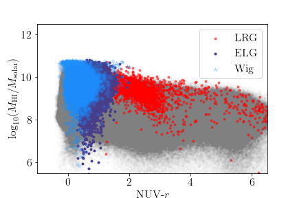
Figure 5: The Hi mass $M_{\rm HI}$ of our mock galaxy lightcone as a function of galaxy colour, $({\rm NUV}-r)$. The full light cone of $N=8.7\cdot 10^{6}$ galaxies with $M_{*}>10^{8.5}M_{\rm sun}$ spanning $0.6<z<1.0$ is represented in grey, and the galaxy samples in coloured dots.

In Figure 5, we present the galaxy colour to Hi mass diagram, where we use the combination of Galex-NUV and SDSS-$r$ filter to project the galaxies onto the red-blue colour scale. The NUV-$r$ colour division has been shown to be a good proxy for the star formation activity of the objects, see e.g. Cortese et al. (2011). We can see that all three samples occupy different spaces in the colour diagram with WiggleZ galaxies testing the bluest, most highly star-forming objects that are also rich in Hi gas. The ELG sample contains slightly less blue systems with lower star formation and also spanning a wider range of Hi masses. The LRG selection incorporates objects more red in colour, however, since objects are supposed to be large and luminous enough for detection at such high redshift, these are still relatively Hi rich.

3 Foreground Subtraction

3.1 FastICA

Fast Independent Component Analysis (FastICA) (Hyvärinen, 1999) is one of the most popular methods for 21cm foreground cleaning and has been tested on simulated data (Chapman et al., 2012; Wolz et al., 2014; Cunnington et al., 2019) as well as real data from the GBT (Wolz et al., 2016b) and LOFAR (Hothi et al., 2020). As with most foreground removal methods, FastICA exploits the fact that the foregrounds dominated by synchrotron and free-free emission smoothly scale in the line-of-sight direction (frequency) (Oh & Mack, 2003; Seo et al., 2010; Liu & Tegmark, 2011), whereas the Hi signal from the Large Scale Structure follows a near-Gaussian approximation with frequency. We apply FastICA to the GBT intensity mapping data cube in order to remove the foregrounds and non-Gaussian systematics and noise. We provide a brief summary of the method here, and refer the interested reader to Wolz et al. (2014); Wolz et al. (2016b) for more details.

FastICA is a blind component separation method designed to divide a mixture of signals into its individual source components, commonly referred to as the “Cocktail Party problem”. It operates on the assumption that the observed signal is composed of statistically independent sources which are mixed in a linear manner. More specifically, the technique solves the linear problem

$$\boldsymbol{x}=\mathbf{A}\boldsymbol{s}+\epsilon=\sum_{i=1}^{N_{\rm{IC}}}\boldsymbol{a_{i}}s_{i}+\epsilon,$$ (3)

where $\boldsymbol{x}$ is the mixed signal, $\boldsymbol{s}$ represents the $N_{\rm IC}$ independent components (ICs), and $\mathbf{A}$ the mixing matrix. $\epsilon$ is the residual of the analysis. The amplitude of each IC $s_{i}$ is given by the mixing modes $\boldsymbol{a_{i}}$. FastICA separates the signal into components by using the Central Limit theorem, such that the non-Gaussianity of the probability density function of each IC is maximized. This implies that FastICA by definition only incorporates data into $\mathbf{A}\boldsymbol{s}$ that will maximise the non-Gaussianity. The residual $\epsilon$ is obtained by subtracting the $N_{\rm IC}$ components from the original data and this should contain mostly Gaussian-like signal.

In our application of FastICA, the input data is of dimension $N_{\rm pix}\times N_{\nu}$ and the algorithm constructs the mixing matrix $\mathbf{A}$ with dimension $N_{\rm IC}\times N_{\nu}$ and the ICs $\boldsymbol{s}$ with dimension $N_{\rm pix}\times N_{\rm IC}$.

FastICA incorporates any features with frequency correlation, such as point sources, diffuse foregrounds and non-Gaussian noise and systematics into the ICs. It also identifies frequency-localised RFI contributions with weak correlations, as they usually exhibit strong non-Gaussian spatial features. The residual of the component separation should, in theory, only contain the Hi signal and the Gaussian telescope noise.

The number of ICs ($N_{\rm IC}$) used in the component separation is a free parameter and can not be determined by FastICA. In the following sub-sections, we carefully examine the sensitivity of the foreground-subtracted data to different choices of $N_{\rm IC}$, ensuring that our results do not depend on this choice.

3.2 Transfer Function

Foreground subtraction with FastICA and its applications to simulations has been thoroughly investigated by many studies (Wolz et al., 2014; Alonso et al., 2015; Asorey et al., 2020; Cunnington et al., 2021), but the vast majority of simulations published to date have been highly idealised and do not included any instrumental effects other than Gaussian noise. In this idealised setting, FastICA has been found to very effectively remove foregrounds for low numbers of ICs starting from $N_{\rm IC}=4$. We note that these numbers also depend on the sophistication of the foreground models, for example, see Cunnington et al. (2021) for $N_{\rm IC}>4$ in the case where polarisation leakage is included in the simulations.

FastICA applied to systematics dominated data can effectively remove non-Gaussian and anisotropic systematics (Wolz et al., 2016b), as well as the astrophysical foregrounds. This means that for increasing $N_{\rm IC}$, the algorithm incorporates more subtle signals as well as more local features into the components. This can significantly reduce the presence of noise and systematics in the data, however, it could also lead to Hi signal loss.

In the following, we investigate the signal loss for different numbers of $N_{\rm IC}$ in the presence of systematics and use the methodology presented in Switzer et al. (2015) to construct the transfer function to correct for Hi signal loss. In absence of a telescope simulator for the (unknown) systematics, we obtain the transfer function by injecting mock Hi signal from simulations into the observed maps before foreground removal. We then process the combined maps with FastICA, and determine the Hi signal loss by cross-correlating the cleaned maps with the injected Hi simulation. In order to reduce noise, we use the average of 100 Hi realisations and we also subtract the cleaned GBT data from the combined data before cross-correlating with the injected signal.

We describe the process in detail below:

• We create $N_{m}=100$ mock simulations $m_{i}$ of lognormal halo distributions using the python package powerbox (Murray, 2018) with a halo mass limit of $M_{h,{\rm min}}=10^{12.3}M_{\odot}/h$.

• We populate each dark matter halo with a Hi mass following a simple Hi halo mass relation as in Wolz et al. (2019).

• We grid the Hi mass of each halo to the same spatial and frequency resolution as the GBT data at median redshift $z\approx 0.8$.

• We convert the Hi grid into brightness temperature $T_{\rm HI}$ using Equation 1, re-scale the overall averaged temperature to the same order of magnitude as the theory prediction with $\Omega_{\rm HI}=0.5\times 10^{-3}$, and convolve the data with a constant, symmetric Gaussian beam with ${\rm FWHM}=0.44\deg$.

• We add each mock Hi brightness temperature realisation $m_{i}$ to each GBT season $j\in\{A,B,C,D\}$ of the GBT data to create combined cubes $(d_{j}+m_{i})$.

• We run FastICA with $q$ number of independent components on each sub-dataset as ${\rm ICA}_{q}(d_{j}+m_{i})$, where $q\in\{4,8,20,36\}$.

• We subtract the original, cleaned GBT data cube to obtain the cleaned mock simulations $\tilde{m}_{qi}^{j}={\rm ICA}_{q}(d_{j}+m_{i})-{\rm ICA}_{q}(d_{j})$ for each realisation $i$, each GBT season $j$ and each choice of foreground removal $N_{\rm IC}=q$.

A comparison of the amplitudes and shapes of the auto-power spectrum of the foreground cleaned injected mock $\tilde{m}_{qi}^{j}$ and auto-power spectrum of the original mock $m_{i}$ measures the Hi signal loss of the power spectrum through the foreground removal. However, in this study, we are interested in quantifying the Hi signal loss through foreground subtraction on the cross-correlation power spectrum with galaxy surveys. In order to approximate this effect, we examine the cross-power spectrum of the foreground removed mock $\tilde{m}_{qi}^{j}$ with the original mock $m_{i}$, where the original mock acts as approximate of the galaxy field with cross-correlation coefficient equal to unity. We define the signal loss function $\Delta$ per season $j$ for different $q=N_{\rm IC}$ averaged over all realisations as

$$\Delta^{j}_{q}(k)=\frac{\sum_{i}^{{N_{m}}}P(\tilde{m}_{q,i}^{j},m_{i})(k)}{\sum_{i}^{N_{m}}P(m_{i})(k)}\,.$$ (4)

In an ideal situation without any signal loss, $\Delta^{j}_{q}(k)$ is equal to unity across all scales. Note that here, $\Delta$ is defined as the Hi signal loss function on the Hi-galaxy cross-correlation.

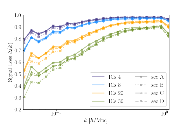
Figure 6: The signal loss function $\Delta(k)$ for the foreground subtraction with FastICA for different numbers of ICs $N_{\rm IC}$. Note that $\Delta=0.8$ means $20\%$ signal loss. We show the the individual seasons $\rm\{A,B,C,D\}$ to highlight the sensitivity of the transfer function to the individual season-dependent systematics.

In our analysis, the signal loss is corrected via the transfer function of the cross-correlation defined as $\Theta^{j}_{q}=(\Delta^{j}_{q})^{-1}$. We show the signal loss function in Figure 6. For all tested $N_{\rm IC}$, there is some significant degree of signal loss ranging between $10\%-50\%$ on the largest scales $k<0.1\,h{\rm Mpc^{-1}}$. This can be explained considering the survey geometry, as these scales are mostly tested by line-of-sight modes which are highly affected by diffuse foreground subtraction. Even for increasing numbers of ICs in the subtraction, the transfer function converges towards unity on smaller scales. However, for very high number $N_{\rm IC}=36$, there is signal loss on all scales of the power spectrum. Note that the divergent behaviour from $k>1h{\rm Mpc}^{-1}$ is due to the effect of the beam on these scales, and they are not considered in our final analysis. We can see that in general, the amplitude of the transfer function of season B is somewhat higher than the others, which suggests that this season might suffer more from systematic effects.

4 Power spectrum Results

We use the inverse-noise weighted power spectrum estimator as described in Wolz et al. (2016b). For the cross-correlation of two tracers $a$ and $b$, that is:

$$\hat{P}^{ab}(\vec{k}_{l})=\frac{V\mathrm{Re}\{\tilde{\delta}^{a}(\vec{k}_{l})\cdot\tilde{\delta}^{b}(\vec{k}_{l})^{*}\}}{\sum_{j=1}^{N_{\rm pix}}w^{a}(\vec{x}_{j})\cdot w^{b}(\vec{x}_{j})}\,,$$ (5)

with $\tilde{\delta}$ the Fourier transform of the weighted density field $w(\vec{x}_{j})\delta(\vec{x}_{j})$ of the tracer, $N_{\rm pix}$ the total number of pixels, $w(\vec{x}_{j})$ the weighting function, and $V$ the survey volume. For Hi intensity maps, $w(\vec{x}_{j})$ is given by the inverse noise map of each season. For galaxy surveys, the total weighting factor is $w(\vec{x}_{j})=W(\vec{x}_{j})w_{\rm opt}(\vec{x}_{j})$, where $w_{\rm opt}(\vec{x}_{j})$ is given by optimal weighting function $w_{\rm opt}(\vec{x}_{i})=1/(1+W(\vec{x}_{i})\times\bar{N}P_{0})$, with $P_{0}=10^{3}h^{-3}\rm{Mpc}^{3}$, and the selection function $W(\vec{x}_{j})$. We derive the selection function for each sample from binning the random catalogues. The redshift evolution of these is shown as dashed lines in Figure 3, and the spatial footprint in Figure 2. We note, that we do not use any additional weighting functions for the galaxy power spectrum.

Equation 5 holds for Hi-auto, galaxy-auto, as well as Hi-galaxy correlations. For galaxy power spectra, we additionally remove the shot noise weighted by the selection function as described in Blake et al. (2011). The 1-d power spectra $\hat{P}(k)$ are determined by averaging all modes with $k=|\vec{k}|$ within the $k$ bin width.

In the following, we use $\hat{P}$ to indicate the estimated power spectrum, and $P$ for the theory prediction. All power spectra are estimated using the redshift range $0.62<z<0.95$ with $N_{\nu}=190$, and spatial resolution $N_{\rm RA}=187$ and $N_{\rm DEC}=89$. We use the flat sky approximation at mid-redshift $z=0.78$, resulting in a volume of $V=4.2\cdot 10^{7}({\rm Mpc}/h)^{3}$. Note, that we do not correct for gridding effects with our power spectrum estimator since the power spectrum is dominated by the beam from $k\sim 1\,h{\rm Mpc}^{-1}$.

4.1 Hi Power Spectrum

In this section, we present the Hi power spectrum to visualise the impact of the foreground subtraction and the transfer function. In Figure 7, we show the Hi power spectrum in auto-correlation $\hat{P}_{\rm HI}^{i}$ for each season $i$, as well as the cross-correlation between the seasons $\hat{P}_{\rm HI}^{ij}$ for all investigated numbers of ICs $N_{\rm IC}\in\{4,8,20,36\}$. We present the Hi power spectrum with foreground subtraction correction, where we use $\Theta^{2}_{i}$ as an approximation to correct the auto-power spectrum $i$, and $\Theta_{i}\Theta_{j}$ to correct for the cross-season correlation $ij$.

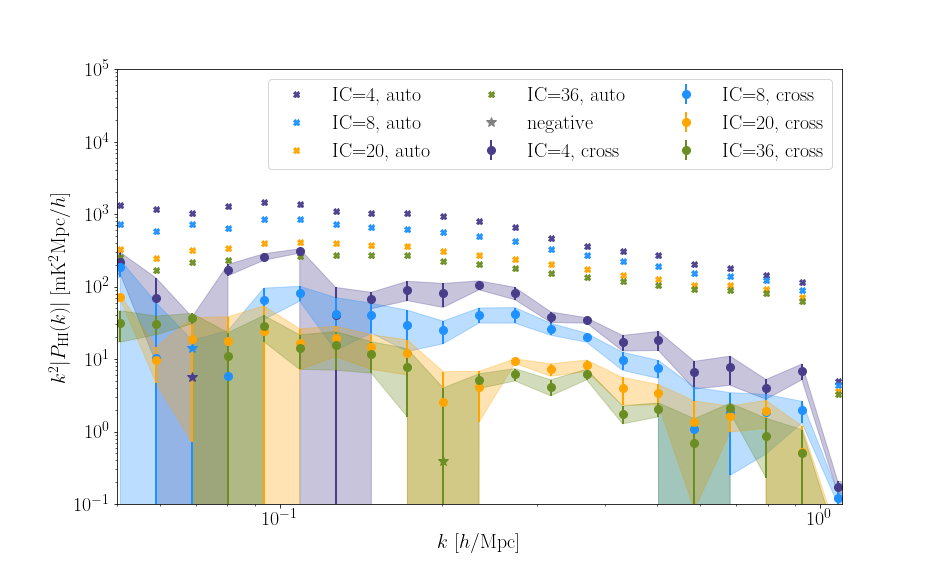
Figure 7: The absolute value of the Hi power spectrum of the GBT intensity maps for different number of ICs in the foreground subtraction. All power spectra are transfer function corrected. We show the auto-correlation between the seasons marked with crosses, and the season cross-correlation with circles. There are a few negative data points (indicated by stars), which demonstrate the high noise on the measurements. Note that these measurements are about an order of magnitude higher than theory predictions and should be treated as upper limits which is in agreement with (Switzer et al., 2015).

As expected, the auto-power spectrum is dominated by instrument noise whose amplitude is higher than the Hi signal. Unlike other subtraction techniques like PCA, FastICA cannot remove and mitigate effects of Gaussian telescope noise. Hence, $P_{\rm HI}^{i}$ can be used as an estimate for the noise present in the data and we use the averaged auto-power spectrum $\hat{P}_{\rm HI,q}^{\rm auto}(k)=\sum_{i}^{4}\hat{P}_{\rm HI,q}^{i}(k)/4$ to estimate the error bars on the Hi power spectrum as:

$$\sigma_{\rm HI,q}(k)=\hat{P}_{\rm HI,q}^{\rm auto}(k)/\sqrt{2N_{\rm modes}}\,,$$ (6)

with $N_{\rm modes}$ the number of $k$ modes sampled in the survey volume, and $q$ the number of ICs, $N_{\rm IC}$. As we use the auto-correlation between seasons as proxy for the noise on the Hi power spectrum, an extra scaling of $\sqrt{2}$ is applied to the error between seasons.

Another way to estimate the noise directly from the data, is using the scatter between cross-season power spectra as noise estimate, and we find that the standard deviation of cross-season is the same order of magnitude as the auto-power spectrum, however, given the limited number of independent seasons, the auto-power spectrum is much less sensitive to sampling variance. For a comparison of these two approaches on the GBT data, please refer to Fig 8 of (Wolz et al., 2016b).

The cross-season power spectra contain a few negative data points, which are indicated by stars in Figure 7. This is the result of the high noise properties in the map which can dominate certain scales.

For the cross-season power spectra, we can see that the amplitude of the spectra is starting to converge for increasing number of $N_{\rm IC}$ on all scales. We are therefore confident that these two choices of ICs in the foreground subtraction are removing sufficient foregrounds. We use $N_{\rm IC}=20$ as a conservative choice with minimal Hi signal loss, and possibly higher residual systematics and noise. Whereas $N_{\rm IC}=36$ is a more assertive choice in the subtraction resulting in lower noise properties with higher levels of Hi signal loss.

4.2 Galaxy Power spectrum

In Figure 8, we show the galaxy power spectra $\hat{P}_{\rm g}(k)$ of our samples in auto- as well as cross-correlation. Note that our power spectrum estimator is not optimised for galaxy surveys and we do not use the galaxy power spectra for a quantitative analysis. Only the auto-galaxy power spectra are shot noise removed, as we do not assume a sample overlap between galaxy surveys.

The error bars on the auto-correlation are estimated as

$$\sigma_{\rm g}(k)=\frac{1}{\sqrt{N_{\rm modes}}}\left(\hat{P}_{\rm g}(k)+\frac{1}{n_{\rm g}}\right)\,,$$ (7)

where $N_{\rm modes}$ is again the number of independent $k$ modes in the survey volume, and $n_{\rm g}$ is the galaxy density of the samples, computed as $n_{\rm g}=N_{\rm g}/V$, with $N_{\rm g}$ the number of galaxies and $V$ the survey volume. The cross-galaxy error bars are estimated as

$$\sigma_{\rm g}^{ij}(k)=\frac{1}{\sqrt{2N_{\rm modes}}}\sqrt{\hat{P}_{\rm g}^{ij}(k)^{2}+\left(\hat{P}_{\rm g}^{i}(k)+\frac{1}{n_{\rm g}^{i}}\right)\left(\hat{P}_{\rm g}^{j}(k)+\frac{1}{n_{\rm g}^{j}}\right)}\,.$$ (8)

In the upper panel of Figure 8, we can see that the ELG and WiggleZ samples are similarly biased across scales, with tentatively an opposite trend in the scale-dependent behaviour. This result is in agreement with theory, as the WiggleZ and ELG samples trace similar populations of galaxies. The bias of the LRG sample is significantly higher, which is again as expected as this sample traces more quiescent, early-type objects in denser environments.

The lower panel of Figure 8 shows the cross-correlation between the galaxy samples, similarly to Anderson et al. (2018). The idea being that the bluer, star-forming samples (ELG and WiggleZ) trace the dark matter in a similar manner to Hi, therefore the shape of the blue-red correlation power spectrum could also be used as a qualitative estimate of the Hi-LRG cross power spectrum. In our data, most notably, the WiggleZ-LRG power spectrum exhibits a drop in amplitude for smaller scales which is not seen for the other two spectra.

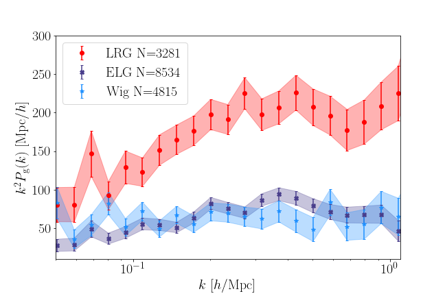
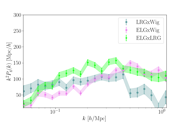
Figure 8: The galaxy power spectrum of the eBOSS LRG, eBOSS ELG and WiggleZ samples. Top: The auto-power spectra of the individual samples, with higher amplitude in the LRG sample and similar amplitudes of the ELG and WiggleZ samples, reflecting the different biases of the samples. Bottom: The cross-correlation between galaxy samples. We observe a drop in small scale amplitude for the LRG-WiggleZ correlation.

4.3 Hi-Galaxy Power Spectrum

In Figure 9, we present the Hi-galaxy cross-power spectra in absolute power for the three galaxy samples and different numbers of ICs in the foreground subtraction. The error bars on these power spectra are determined by the errors on the galaxy sample, see Equation 7, and the Hi data, see Equation 6, combined as

$$\sigma_{\rm g,HI}^{q}(k)=\frac{1}{\sqrt{2N_{\rm modes}}}\sqrt{\hat{P}_{\rm g,HI}^{q}(k)^{2}+\hat{P}_{\rm HI}^{q}(k)\left(\hat{P}_{\rm g}(k)+\frac{1}{n_{\rm g}}\right)}\,,$$ (9)

with $q$ the number of ICs $\{4,8,20,36\}$. We note that the Hi data errors dominate the total cross-power error budget. We discuss errors and covariances in more detail in subsection 4.5 and Appendix B.

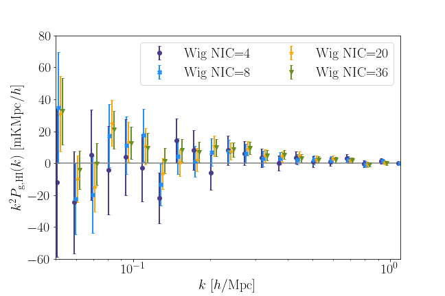
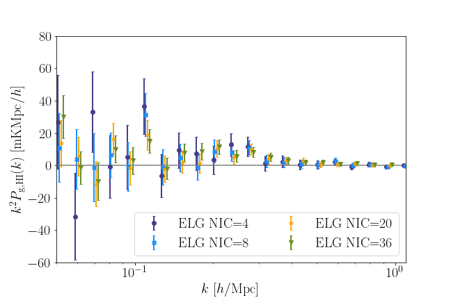
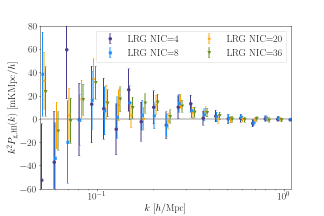
Figure 9: The GBT Hi intensity mapping cross-correlation with the galaxy samples for different numbers of ICs in the foreground subtraction. Note that all power spectra were estimated at the same $k$, and the staggered $k$ values in the plots are for illustration purposes only. From top to bottom: Hi-WiggleZ, Hi-ELG, and Hi-LRG cross-correlation power spectrum.

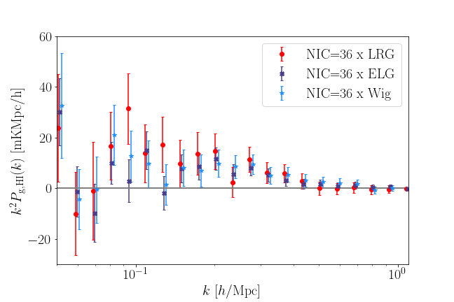
Figure 10: The GBT Hi intensity mapping cross-correlation with the galaxy samples in comparison. Note that all power spectra were estimated at the same $k$, and the staggered $k$ values in the plots are for illustration purposes only.

We can see in all three panels of Figure 9, that the amplitude of the cross-power signal is not very sensitive to the foreground removal parameters within the error bars. We do not observe a drop in amplitude with increasing numbers of ICs, and we are confident that we correctly account for Hi signal loss with our transfer function, particularly, within the large errors of the GBT data. Generally, as the amplitude of the noise of the GBT data is decreased with increasing $N_{\rm IC}$, the detection of the signal becomes more statistically significant and the error bars decrease with increasing components removed. In Figure 10, we show the cross-correlation of the three galaxy samples for fixed $N_{\rm IC}=36$ in comparison.

The GBT-WiggleZ cross-correlation in the upper panel of Figure 10, is detected for both $N_{\rm IC}=20,36$ on scales $0.1<k<0.8\,h{\rm Mpc}^{-1}$. Qualitatively, the middle panel showing the amplitude of the GBT-ELG correlation looks very similar, but the detection seems more noise dominated on the larger scales, around $k\approx 0.1h{\rm Mpc}^{-1}$. The GBT-LRG correlation shown in the lowest panel demonstrates a detection of the signal for $N_{\rm IC}=36$. At the smallest scales around $k\sim 1\,h{\rm Mpc}^{-1}$, the amplitude of the correlation signal drops off and the power spectrum is highly noise dominated. Anderson et al. (2018) reported a drop in amplitude in the cross-correlation of the Parkes Hi intensity maps with the red sub-sample 2dF galaxies. However, the signal-to-noise ratio of the GBT-LRG measurements is not large enough to confirm this trend.

The cross-correlation of WiggleZ-LRG galaxies as shown in Figure 8 supports that this would be an expected result for our data. The negligible power of the correlation of the Hi intensity maps with the LRG galaxy sample on small scales, implies that the LRG galaxies that contribute to these scales are Hi deficient. The power spectrum signal on these scales originates from galaxy pairs most likely part of the same halo in a dense cluster environment. The Hi deficiency of these types of quiescent galaxies has been predicted in theory and observed for the local Universe(Reynolds et al., 2020). Our work is an indicator for this trend for cosmological times.

We will make more quantitative estimates for the significance of the detections when we present our derived Hi constraints in Section 5.

4.4 Comparison to Simulations

We use our simulations for qualitative interpretation of our results. We use the same redshift range with $\bar{z}\approx 0.78$ to estimate the power spectra of our mock data, however, we do not mask the edges of the data which results in a bigger volume of $V=4.8\cdot 10^{7}({\rm Mpc}/h)^{3}$. We do not include any noise and instrumental effects in this simulation suite as we focus on understanding the implication from galaxy evolution on the cross-correlation signal.

In Figure 11 from top to bottom, we show the power spectra for the galaxy samples, the cross-galaxy and the Hi-galaxy correlations. The shapes and amplitudes of the galaxy power spectrum are comparable to the data power spectrum. We presume that the fluctuations of the mock LRG sample are due to the low galaxy density. The cross-galaxy power spectra are comparable to the data measurements, with a drop in amplitude at smaller scales $k>0.8\,h{\rm Mpc}^{-1}$.

In the bottom panel of Figure 11 we show the resulting mock Hi-galaxy cross-correlation. We note that the overall amplitude is lower than the data due to a lower $\Omega_{\rm HI}$ than data measurements suggest. The simulations predict the amplitude of all power spectra at the same level of magnitude. We show the beam-convolved mock as well as a unconvolved power spectrum, to demonstrate the effect of the Hi shot noise, as predicted in Wolz et al. (2017). The amplitude of the cross-shot noise is proportional to the ensemble averaged Hi mass of the respective galaxy sample. Our simulation predicts the highest shot noise amplitude for the Hi-WiggleZ correlation, and very similar levels for both eBOSS samples. However, on the scales unaffected by the GBT telescope beam, the shot noise does not have a measurable effect, in particular when considering the signal-to-noise ratio of our data. Notably, we do not find a drop in amplitude of the Hi-LRG correlation. This could suggest, that the drop could be caused by an unknown observational effect, which we were unable to identify with our tests given the large uncertainties of the data, or, alternatively, that our selection of mock LRG galaxies or the model itself misses some features and our mock sample can not fully represent the data. We hope to investigate this interesting feature in future work with less noise-dominated Hi intensity maps.

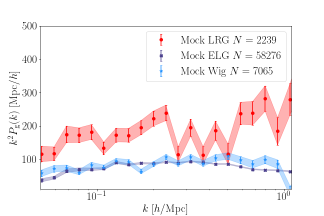
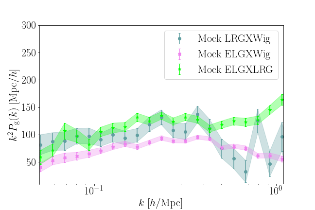
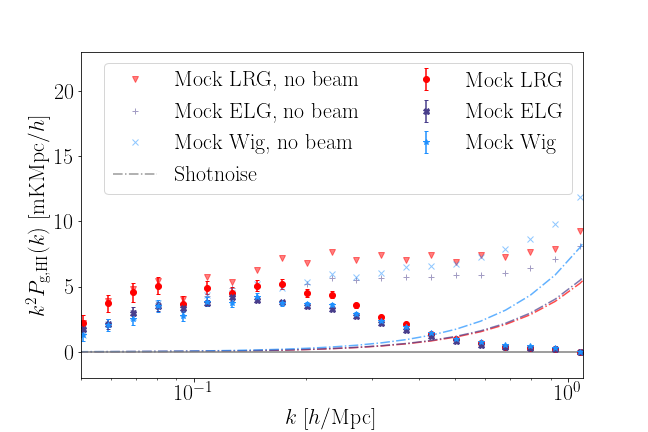
Figure 11: The power spectra of our simulation suite. Top: The auto-galaxy power spectra of the three galaxy samples. The mock-ELG and WiggleZ power spectra are of similar amplitude, whereas the mock-LRG exhibits a higher bias, consistent with the data. Middle: The cross-galaxy power spectra of the mock samples. Similarly to the data, we see a possible drop in amplitude on smaller scales for the LRG-WiggleZ correlation. Bottom: The Hi-galaxy cross-correlation, beam-convolved and with no beam to demonstrate the effect of the cross-shot noise. The dashed-dotted lines indicate the shot noise amplitude.

4.5 Analysis tests

We perform several tests of our analysis pipeline listed in this section. For these tests, we examine the covariance matrix of the mock data computed as

$$\mathbf{C}_{q}=C_{q}(k_{i},k_{j})=\sum_{m}^{N_{m}}\frac{(P_{m}^{q}(k_{i})-\bar{P}^{q}(k_{i}))(P_{m}^{q}(k_{j})-\bar{P}^{q}(k_{j})}{N_{m}}$$ (10)

where the number of independent components $q=\{4,8,20,36\}$, $\bar{P}$ the averaged power spectrum over all realisations, and $N_{m}$ the number of realisations. We can derive an estimate for error bars from the diagonal as $\sigma_{i}^{q}=\sqrt{\mathbf{C}^{q}_{ii}}$. Figures of the resulting covariance matrices and tests can be found in Appendix B.

• Mode correlation from fastICA: We derive the covariance of the data to determine the statistical independence between $k$ bins. We use the power spectra $P(\tilde{m}_{q,i}^{j},m_{i})(k)$ of the foreground-subtracted lognormal simulations $\tilde{m}_{q,i}^{j}$ with the original simulation $m_{i}$, and compute the covariance matrix. We find no significant off-diagonal correlations between the modes $0.05<k<0.8\,h{\rm Mpc}^{-1}$ considered in our analysis. We also compute the errors from the diagonal of the inverted covariance matrix to determine the additional error introduced from the foreground removal. We find that this contribution is more than 2 orders of magnitude lower than the analytical errors based on noise and cosmic variance as determined by Equation 6. We therefore can safely neglect this contribution in the present analysis.

• Randoms null test: We correlate the GBT sub-season data with the $N_{m}=100$ random WiggleZ catalogues used to derive the selection function. As expected, we find a signal consistent with zero within the error bars. We also derive the covariance matrix from the mocks and find that the error bars $\sigma_{\rm cov}$ are in agreement with the empirically derived $\sigma_{\rm g,HI}$ in Equation 9.

• Shuffled null test: We correlate the GBT sub-season data with the three galaxy samples which are each re-shuffled in redshift to remove the correlation. As expected, we find all signals consistent with zero within the error bars.

5 Hi constraints

Here, we are present our derived Hi constraints from the cross-correlation power spectra analysis (summarised in Table 1). Before doing so, we briefly review the findings of Masui et al. (2013), who measured the GBT maps cross-correlation with the WiggleZ 15hr and 1hr fields. Fitting in the range of scales $0.05\,h{\rm Mpc}^{-1}<k<0.8\,h{\rm Mpc}^{-1}$, they found $10^{3}\Omega_{\textrm{H{i}}}b_{\textrm{H{i}}}r=0.40\pm 0.05$ for the combined, $10^{3}\Omega_{\textrm{H{i}}}b_{\textrm{H{i}}}r=0.46\pm 0.08$ for the 15hr field and $10^{3}\Omega_{\textrm{H{i}}}b_{\textrm{H{i}}}r=0.34\pm 0.07$ for the 1hr field (which is the one we are considering in this paper). For a more restrictive range of scales, their combined measurement was $10^{3}\Omega_{\textrm{H{i}}}b_{\textrm{H{i}}}r=0.44\pm 0.07$. Note that Masui et al. (2013) used Singular Value Decomposition (SVD) for their foreground removal, but we use FastICA here following Wolz et al. (2016b). Our transfer function construction methods are identical. We note that the errors quoted are statistical, and Masui et al. (2013) also estimated a $\pm 0.04$ systematic error representing their $9\%$ absolute calibration uncertainty. We will adopt the same systematic error in our analysis.

In this paper we will explore different ranges of scales, by performing fits for three cases: Case I, with $0.05\,h{\rm Mpc}^{-1}<k<0.8\,h{\rm Mpc}^{-1}$. Case II, with $0.05\,h{\rm Mpc}^{-1}<k<0.45\,h{\rm Mpc}^{-1}$, and Case III, with $0.05\,h{\rm Mpc}^{-1}<k<0.35\,h{\rm Mpc}^{-1}$. Considering different ranges of scales is motivated by the fact that, while small scales (high $k$) contain most of the statistical power of the measurement, the beam and model of non-linearities become less robust as $k$ increases.

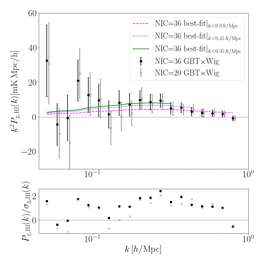
Figure 12: Top: The measured GBT-WiggleZ cross-correlation power spectrum. We show two cases with $20$ and $36$ Independent Components used in FastICA for the Hi maps foreground cleaning, corrected with the corresponding transfer functions. We also show the best-fit models from Table 1 (Cases I, II, and III) for $N_{\rm IC}=36$. Bottom: A null diagnostic test plotting the ratio of data and error.

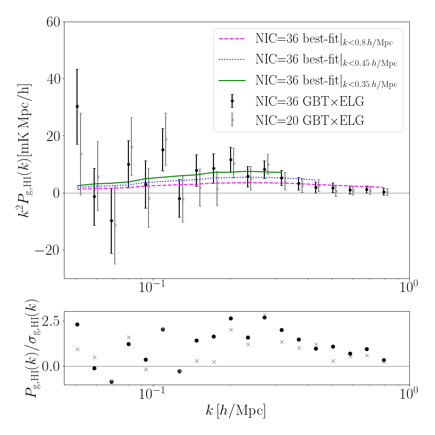
Figure 13: Top: The measured GBT-ELG cross-correlation power spectrum for $N_{\rm IC}=20,36$. We also show the best-fit models from Table 1 (Cases I, II, and III) for $N_{\rm IC}=36$. Bottom: A null diagnostic test plotting the ratio of data and error.

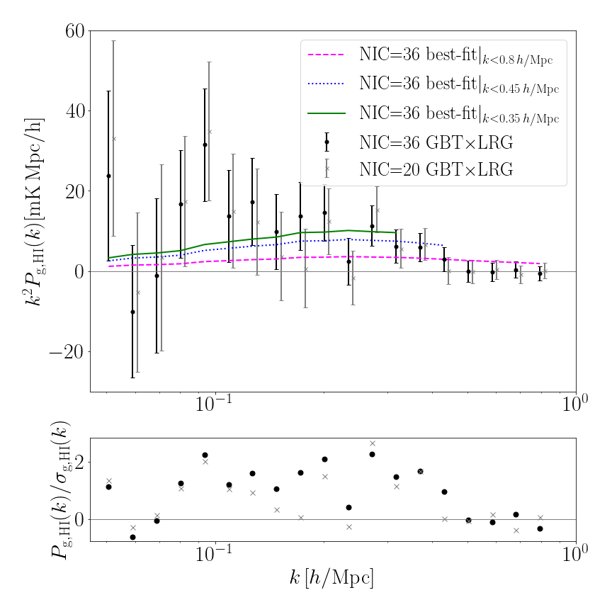
Figure 14: Top: The measured GBT-LRG cross-correlation power spectrum for $N_{\rm IC}=20,36$. We also show the best-fit models from Table 1 (Cases I, II, and III) for $N_{\rm IC}=36$. Bottom: A null diagnostic test plotting the ratio of data and error.

In Figure 12 we show the measured GBT-WiggleZ power spectrum, concentrating on the results with $N_{\rm IC}=20,36$. In the bottom panel, we perform a simple null diagnostic test by plotting the ratio of data and error. This shows that most of the measurements in the range of scales with high signal-to-noise ratio are more than $1\sigma$ positively away from $0$. For our fiducial IC=36 results for Case I, corresponding to the same range of scales considered in Masui et al. (2013), the detection significance is estimated to be $4.4\sigma$ (we note that in Masui et al. (2013) this was found to be $7.4\sigma$ but for the combined 1hr and 15hr fields observations). We show similar plots for the GBT-ELG and GBT-LRG cross-correlations in Figure 13 and Figure 14, respectively. We note that our null tests suggest that the GBT-LRG detection is the most tentative of the three. Indeed, estimating the detection significance for GBT-ELG and GBT-LRG, we find $4.5\sigma$ and $2.9\sigma$, respectively, for Case I. In Table 1 we show the detection significance for $N_{\rm IC}=36$ for all Cases. We see that the detection significance for the GBT-LRG cross-correlation considerably improves when considering the restricted ranges of scales, Cases II and III.

To relate the measured power spectra with a theory model and derive the Hi constraints, we use Equation 1 to express the mean 21cm emission brightness temperature $T_{\textrm{H{i}}}$ as a function of $\Omega_{\textrm{H{i}}}$. We observe the brightness contrast, $\delta T=T_{\textrm{H{i}}}\delta_{\textrm{H{i}}}$. We also assume that the neutral hydrogen and the optical galaxies are biased tracers of dark matter, but we also include a galaxy-Hi stochastic correlation coefficient $r_{\textrm{H{i}},{\rm opt}}$. To compare the theoretical prediction with the measurements, we follow a procedure similar to the one described in Masui et al. (2013):

• We assume a fixed Planck cosmology (Ade et al., 2016).

• We assume a known galaxy bias $b_{\rm opt}$ at the mean redshift $z\simeq 0.8$, with ${\rm opt}$ corresponding to WiggleZ (Blake et al., 2011), eBOSS ELGs, and eBOSS LRGs (Alam et al., 2021) depending on the galaxy sample we cross-correlate the Hi maps with. That is, $b_{\rm Wig}=1.22$, $b_{\rm ELG}=1.4$, $b_{\rm LRG}=2.3$.

• We include non-linear effects to the matter power spectrum $P_{\rm m}(k)$ using CAMB (Lewis et al., 2000) with HALOFIT (Smith et al., 2003; Takahashi et al., 2012) and also include (linear) redshift space distortions as $(1+f\mu^{2})^{2}$ (Kaiser, 1987), where $f$ the growth rate of structure and $\mu$ the cosine of the angle to the line-of-sight. When spherically averaged to compute the matter power spectrum monopole, $P_{\delta\delta}(k)$, this RSD factor gives an amplitude boost of $1.7$ for our fiducial cosmology.

• We then construct an empirical cross-power spectrum model $P_{\textrm{H{i}},{\rm g}}$ given by (Masui et al., 2013):

  $$P_{\textrm{H{i}},{\rm g}}(k)=T_{\textrm{H{i}}}b_{\textrm{H{i}}}b_{\rm g}r_{\textrm{H{i}},{\rm opt}}P_{\delta\delta}(k)\,.$$ (11)

  The model is run through the same pipeline as the data to include weighting, beam, and window function effects, as described in Wolz et al. (2016b). We will comment further on our modelling choices at the end of this section.

• We fit the unknown prefactor $\Omega_{\textrm{H{i}}}b_{\textrm{H{i}}}r_{\textrm{H{i}},{\rm opt}}$ to the data. We perform fits for all three ranges of scales (Cases I, II, and III in Table 1). We find a good reduced chi-squared $\chi_{\rm red}^{2}\sim 1$ for our choice of model in all cases and samples. We also note that excluding the measurements at $k<0.08\,h{\rm Mpc}^{-1}$ (where there are too few modes in the volume) does not make a discernible difference to our results.

• We report our $\Omega_{\textrm{H{i}}}b_{\textrm{H{i}}}r_{\textrm{H{i}},{\rm opt}}$ at three different effective scales $k_{\rm eff}$, which are estimated by weighting each $k$-point in the cross-power by its $(\mathrm{S_{\rm best-fit}/N})^{2}$, for Cases I, II, and III. As we already mentioned, we do this because most of our measurements lie at the nonlinear regime. Assigning an effective scale also allows for a better interpretation of the implications for the values of $r_{\textrm{H{i}},{\rm opt}}$.

Table 1: Best-fit and $1\sigma$ statistical errors on $10^{3}\Omega_{\textrm{H{i}}}b_{\textrm{H{i}}}r_{\textrm{H{i}},{\rm opt}}$ at a mean redshift $z\simeq 0.8$ for $N_{\rm IC}=20,36$, together with the effective scale $k_{\rm eff}$, detection significance, and reduced chi-squared $\chi^{2}_{\rm red}=\chi^{2}/{\rm dof}$

for $N_{\rm IC}=36$ (Cases I, II, and III; see main text for details).
GBT$\times$WiggleZ GBT$\times$ELGs GBT$\times$LRGs $k_{\rm eff}[h/{\rm Mpc}]$ Case I [$k<0.8\,h/{\rm Mpc}$] NIC=20: $0.35\pm 0.09$ $0.20\pm 0.06$ $0.12\pm 0.06$ - NIC=36: $0.38\pm 0.08$ ($4.4\sigma$, $\chi^{2}_{\rm red}\simeq 16/18$) $0.26\pm 0.06$ ($4.5\sigma$, $22.6/18$) $0.16\pm 0.06$ ($2.9\sigma$, $22.9/18$) 0.48 Case II [$k<0.45\,h/{\rm Mpc}$] NIC=20: $0.53\pm 0.12$ $0.36\pm 0.09$ $0.28\pm 0.09$ - NIC=36: $0.58\pm 0.09$ ($4.8\sigma$, $\chi^{2}_{\rm red}\simeq 8.3/14$) $0.40\pm 0.09$ ($4.9\sigma$, $16/14$) $0.35\pm 0.08$ ($4.4\sigma$, $12.3/14$) 0.31 Case III [$k<0.35\,h/{\rm Mpc}$] NIC=20: $0.58\pm 0.17$ $0.48\pm 0.12$ $0.38\pm 0.12$ - NIC=36: $0.70\pm 0.12$ ($4.4\sigma$, $\chi^{2}_{\rm red}\simeq 6.7/12$) $0.55\pm 0.11$ ($5\sigma$, $11.6/12$) $0.45\pm 0.10$ ($4.2\sigma$, $10/12$) 0.24

Our derived constraints are shown in Table 1, for $N_{\rm IC}=20$ and $N_{\rm IC}=36$ (for the smaller $N_{\rm IC}$ cases the errors are too large due to residual foreground variance). In the GBT-WiggleZ Case I, we find excellent agreement with the Masui et al. (2013) results for the 1hr field, $10^{3}\Omega_{\textrm{H{i}}}b_{\textrm{H{i}}}r_{\textrm{H{i}},{\rm Wig}}=0.34\pm 0.07$. Using this case as our benchmark, the lower result in the GBT-ELGs case implies a smaller correlation coefficient between these galaxies and Hi, and even smaller in the GBT-LRGs case. The results imply that red galaxies are much more weakly correlated with Hi on the scales we are considering, suggesting that Hi is more associated with blue star-forming galaxies and tends to avoid red galaxies. The same trend is followed in the restricted ranges of scales Cases II and III, albeit with different derived best-fit amplitudes. This is in qualitative agreement with what was found in Anderson et al. (2018) when separating the 2dF survey sample into red and blue galaxies, albeit at a much lower redshift $z=0.08$. The effective scales of the three Cases are different: Case I has $k_{\rm eff}=0.48\,\,h/{\rm Mpc}$, Case II has $k_{\rm eff}=0.31\,\,h/{\rm Mpc}$, and Case III has $k_{\rm eff}=0.24\,\,h/{\rm Mpc}$. The different derived best-fit amplitudes are within expectation as $r_{\textrm{H{i}},{\rm opt}}$ and $b_{\textrm{H{i}}}$ are predicted to be scale-dependent. Therefore, we also expect that if another survey targets larger (linear) scales, e.g. $k<0.1\,h/{\rm Mpc}$, it will derive different $\Omega_{\textrm{H{i}}}b_{\textrm{H{i}}}r_{\textrm{H{i}},{\rm opt}}$. To illustrate the variation between cases, we also present the $N_{\rm IC}=36$ results in Figure 15.

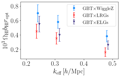
Figure 15: Best-fit and $1\sigma$ statistical errors on $10^{3}\Omega_{\textrm{H{i}}}b_{\textrm{H{i}}}r_{\textrm{H{i}},{\rm opt}}$ at a mean redshift $z\simeq 0.8$ for $N_{\rm IC}=36$, together with the effective scale $k_{\rm eff}$ (staggered for illustration purposes).

We can proceed with the interpretation of our results making some further assumptions. First of all, since the correlation coefficient $r<1$, our results put a lower limit on $\Omega_{\textrm{H{i}}}b_{\textrm{H{i}}}$. It would also be interesting to attempt to determine $\Omega_{\textrm{H{i}}}$ from our measurements taking some external estimates for $b_{\textrm{H{i}}}$ and $r_{\textrm{H{i}},{\rm opt}}$. The linear bias of Hi is expected to be $\sim 0.65$ to $\sim 1$ at these redshifts (Marin et al., 2010), and we will assume $r_{\rm\textrm{H{i}},Wig}=0.9$ (Khandai et al., 2011). Using our simulations (taking their ratios at $k_{\rm eff}$ for Case III, which is the case where non-linearities are expected to be milder), we can estimate $r_{\rm\textrm{H{i}},ELG}\sim 0.7$ and $r_{\rm\textrm{H{i}},LRG}\sim 0.6$. Combining these values with the results in Table 1 and our assumption of perfect knowledge of the galaxy samples biases, we get the $\Omega_{\textrm{H{i}}}$ estimates shown in Figure 16. These are shown together with other available constraints from the literature (Braun, 2012; Zwaan et al., 2005; Rao et al., 2006; Lah et al., 2007; Martin et al., 2010; Rhee et al., 2013; Hoppmann et al., 2015; Rao et al., 2017; Jones et al., 2018; Bera et al., 2019; Hu et al., 2019; Chowdhury et al., 2020). For recent compilations of $\Omega_{\textrm{H{i}}}$ measurements in the redshift range $0<z<5$, see Crighton et al. (2015); Neeleman et al. (2016); Hu et al. (2019) .

As a final note, we caution the reader that these estimates are crude given the number of assumptions we have made. In principle, the degeneracy between $\Omega_{\textrm{H{i}}}$ and $b_{\textrm{H{i}}}$ can be broken with the use of redshift space distortions (Wyithe, 2008; Masui et al., 2013), but we need higher quality Hi intensity mapping data with a much better signal-to-noise ratio to achieve this (Masui et al., 2010; Pourtsidou et al., 2017). We also stress that while our empirical model (Equation 11) has provided an acceptable statistical fit to our data sets, it is not appropriate for high-precision future data. Following what is done in optical galaxy surveys (see e.g. Blake et al. (2011); Beutler et al. (2014)), with better data we would need to use more sophisticated models and perform a comprehensive Hi power spectrum multipole expansion analysis (Cunnington et al., 2020). For example, for the cross-correlation case a more appropriate model to use would be:

$$P_{\textrm{H{i}},g}(k,\mu)=T_{\textrm{H{i}}}b_{g}b_{\textrm{H{i}}}\frac{[r_{\textrm{H{i}},{\rm opt}}+(\beta_{\textrm{H{i}}}+\beta_{g})\mu^{2}+\beta_{\textrm{H{i}}}\beta_{g}\mu^{4}]}{1+(k\mu\sigma_{v}/H_{0})^{2}}P_{\rm m}(k)\,,$$ (12)

with $\beta_{i}=f/b_{i}$ and $\sigma_{v}$ the velocity dispersion parameter. Further, to appropriately model the power spectrum at scales above $k\sim 0.15\,h{\rm Mpc}^{-1}$ at $z\sim 1$ we would also need to account for scale-dependent bias and $r_{\textrm{H{i}},{\rm opt}}$, and construct perturbation theory based models (Villaescusa-Navarro et al., 2018; Castorina & White, 2019) including observational effects (Blake, 2019; Soares et al., 2021). To summarise, with our currently available measurements we are very constrained in the number of parameters we can simultaneously fit, and we cannot break any degeneracies unless we use several assumptions and external estimates, hence our empirical choice of model. Furthermore, for precision cosmology studies with future data we will need to take into account the cosmology dependence of the transfer function (Soares et al., 2021).

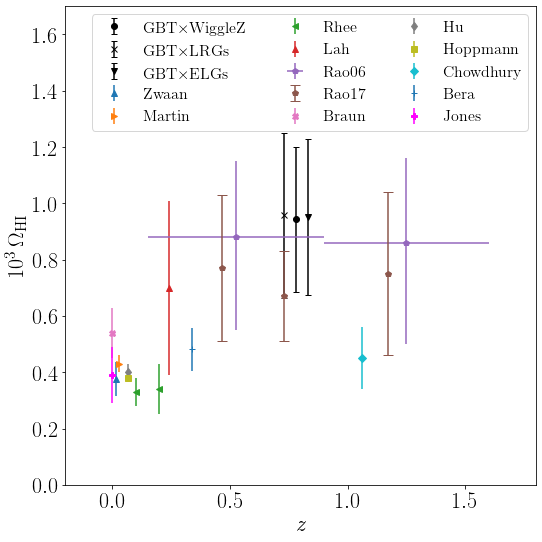
Figure 16: Estimates for $\Omega_{\textrm{H{i}}}$ from this work compared to other measurements in the literature. All our estimates are at the central redshift $z=0.78$ but they have been staggered for illustration purposes. We used the results from Table 1 Case III ($k_{\rm eff}=0.24\,h/{\rm Mpc}$) for deriving these estimates. Masui et al. (2013) estimated $10^{3}\Omega_{\textrm{H{i}}}$ between $0.45$ and $0.75$

. Our assumptions and methodology are detailed in the main text.

6 Conclusions

In this work, we performed the first ever comparison of the Hi intensity mapping detections in cross-correlation with multiple galaxy surveys. We use an extended version of the previously published GBT Hi intensity mapping data located in the 1hr field in combination with the WiggleZ Dark Energy Galaxy survey, and the SDSS eBOSS ELG and LRG samples.

For the GBT data, we subtract the foregrounds and mitigate some systematics via FastICA for $N_{\rm IC}\in\{4,8,20,36\}$. In addition, for the first time for FastICA, we construct a transfer function for the Hi signal loss via mock simulations. We find that there can be a high signal loss up to $50\%$ for $k<0.2\,h{\rm Mpc}^{-1}$, as foreground removal affects the line-of-sight modes on these scales for all $N_{\rm IC}$. The transfer function converges towards unity for smaller scales, however, for $N_{\rm IC}=36$, we find there is a minimum of $20\%$ signal loss on all scales. The amplitude of the transfer function varies between seasons, indicating that the systematics strongly affect the Hi signal loss.

For the Hi intensity mapping auto-power spectrum, we find that the amplitude of the cross-season power spectrum converges for increasing number of ICs. The amplitude is in agreement with previous work in Masui et al. (2013); Switzer et al. (2013); Wolz et al. (2016b), and should be interpreted as an upper limit for detection.

We investigate the shapes of the galaxy cross-power spectrum, particularly, the correlation between the WiggleZ and the LRG data. We observe a drop in amplitude on the small scales $k\approx 0.8$ for the LRG-Wigglez correlation, which can be assumed as a proxy for the Hi-LRG correlation, as WiggleZ galaxies are assumed to be Hi -rich and hence a similar tracer to Hi intensity maps. We find that the amplitudes of the Hi-galaxy cross-correlations do not strongly depend on the $N_{\rm IC}$ of our foreground subtraction. We find a significant drop in amplitude in the Hi-LRG correlation at large scales, in agreement with previous findings in Anderson et al. (2018).

We construct a mock data set including Hi information and optical galaxy magnitudes based on the outputs of the semi-analytic model DARKSAGE and qualitatively compare the results to our data. Our mock catalogues predict the WiggleZ sample to contain the Hi-richest galaxies. Due to the selection of bright objects, the LRG sample also has relatively Hi-rich objects, and the averaged mass is in a similar range as the ELG sample. The simulations confirm a drop in amplitude in the LRG-WiggleZ correlation, but not in the Hi-LRG correlation. This could be due to failure of our simulation (not matching selection of our galaxies), or the decrease in amplitude caused by observational effects. The present signal-to-noise ratio is not high enough to investigate this further.

Finally, we use the cross-correlation measurements to constrain the quantity $\Omega_{\textrm{H{i}}}b_{\textrm{H{i}}}r_{\textrm{H{i}},{\rm opt}}$, where $\Omega_{\textrm{H{i}}}$ is the Hi density fraction, $b_{\textrm{H{i}}}$ is the Hi bias, and $r_{\textrm{H{i}},{\rm opt}}$ the galaxy-hydrogen correlation coefficient. We consider three different ranges of scales, which correspond to three different effective scales $k_{\rm eff}$ for our derived constraints. At $k_{\rm eff}=0.31\,h/{\rm Mpc}$ we find $\Omega_{\textrm{H{i}}}b_{\textrm{H{i}}}r_{\textrm{H{i}},{\rm Wig}}=[0.58\pm 0.09\,{\rm(stat)\pm 0.05\,{\rm(sys)}}]\times 10^{-3}$ for GBT-WiggleZ, $\Omega_{\textrm{H{i}}}b_{\textrm{H{i}}}r_{\textrm{H{i}},{\rm ELG}}=[0.40\pm 0.09\,{\rm(stat)\pm 0.04\,{\rm(sys)}}]\times 10^{-3}$ for GBT-ELG, and $\Omega_{\textrm{H{i}}}b_{\textrm{H{i}}}r_{\textrm{H{i}},{\rm LRG}}=[0.35\pm 0.08\,{\rm(stat)\pm 0.03\,{\rm(sys)}}]\times 10^{-3}$ for GBT-LRG, at $z\simeq 0.8$. We also report results at $k_{\rm eff}=0.24\,h/{\rm Mpc}$ and $k_{\rm eff}=0.48\,h/{\rm Mpc}$. The best-fit amplitudes and $1\sigma$ statistical errors for all these cases are shown in Table 1. Our results are amongst the most precise constraints on neutral hydrogen density fluctuations in a relatively unexplored redshift range, using three different galaxy samples.

Our findings as well as our developed simulations and data analysis pipelines will be useful for the analysis of forthcoming Hi intensity mapping data, and for the preparation of future surveys.

Data Availability

The raw GBT intensity mapping data (the observed time stream data) is publicly available according to the NRAO data policy, which can be found at https://science.nrao.edu/observing/proposal-types/datapolicies. The data products, such as maps and foreground removed maps, will be shared on reasonable request to the corresponding author. We foresee a public release of the GBT data products once the analysis of the maps is finalised and the results are published in scientific journals. The SDSS-IV DR16 data is available at https://www.sdss.org/dr16/.

The DR16 LSS catalogues are publicly available: https://data.sdss.org/sas/dr16/eboss/lss/catalogs/DR16/.

Appendix A Sample selection for optical mock galaxies

For our sample selection in the simulation, we use the selection which includes the magnitude limits of the observations as well as the target selection.

For WiggleZ, we use the selection cuts outlines in Drinkwater et al. (2010), as we have previously done in Wolz et al. (2016b). The selection is based on the GALEX UV filters NUV and FUV, as well as the SDSS $r$ filter, as follows.

$$\begin{split}{\rm NUV}&<22.8\\ 20&<r<22\\ -0.5&<({\rm NUV}-r)<2.\end{split}$$ (13)

For eBOSS ELG, we follow

$$\begin{split}21.825<&g<22.825\\ (-0.068(r-z)+0.457)<&(g-r)<(0.112(r-z)+0.773)\\ (0.218(g-r)+0.571)<&(r-z)<(-0.555(g-r)+1.901).\end{split}$$ (14)

For eBOSS LRG, we follow , where we use the infra red filter IRAC1 as a close approximation for the WISE filter.

$$\begin{split}(19.9<&i<21.8)\\ (&z<19.95)\\ (&{\rm IRAC1}<20.299)\\ &(r-i)>0.98)\\ &(r-{\rm IRAC1})>2(r-i)).\end{split}$$ (15)

Appendix B Covariance and Error estimates

Here we show the covariances and error estimates as described in subsection 4.5.

In Figure 17 we show the covariance based on the cross-power spectra of the 100 lognormal realisations (after injected into the GBT data and cleaned with fastICA) with the original lognormal realisations, see subsection 3.2 and subsection 4.5 for details. We can see that the application of fastICA does not introduce any significant correlations between $k$-modes or off-diagonal elements.

In Figure 18, we show the covariance based on the GBT data with the 100 WiggleZ random catalogues as described in subsection 3.2. We can see that for lower number of ICs, there are non-negligible off-diagonal elements for small $k$-modes, and particularly for $N_{\rm IC}=4$, the amplitude of the off-diagonal elements is increased. Note that the covariance in this work includes both cosmic variance as well as variance from the noise as we average over 100 realisations as well as over the 4 independent GBT data sections.

In Figure 19, we show the comparison of the errorbars resulting from Equation 9 and the diagonal of the covariance matrix based on the GBT data with the WiggleZ randoms as shown in Figure 18. We can see that for small $k$-modes, the error estimate based on the errors from the estimated auto-powerspectra in Equation 9 is higher than the covariance-based estimate, and both estimates converge towards smaller scales.

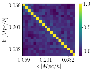
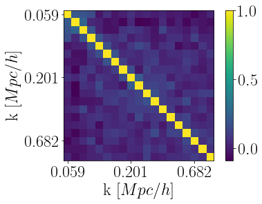
Figure 17: The covariance matrix computed from the power spectrum of the foreground removed lognormal realisations with the original lognormals, as described in subsection 3.2 with clockwise increasing numbers of ICs $N_{\rm IC}$. Upper left panel: $N_{\rm IC}=4$; Upper right panel: $N_{\rm IC}=8$; Lower left panel: $N_{\rm IC}=20$; Lower right panel: $N_{\rm IC}=36$. For illustrative purposes the diagonals of the covariance matrices have been normalised to unity; i.e. the correlation matrix is pictured.

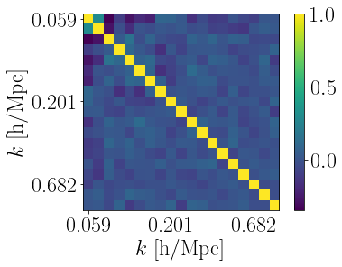
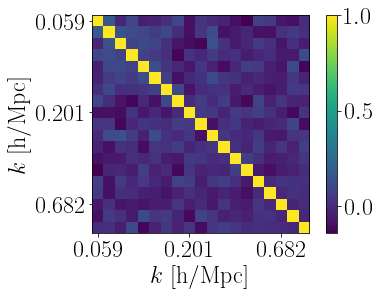
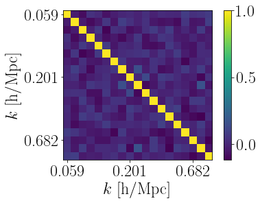
Figure 18: The covariance matrix computed from the cross-correlation of the foreground removed GBT data with WiggleZ random catalogues, as described in subsection 4.5 with clockwise increasing numbers of ICs $N_{\rm IC}$. Upper left panel: $N_{\rm IC}=4$; Upper right panel: $N_{\rm IC}=8$; Lower left panel: $N_{\rm IC}=20$; Lower right panel: $N_{\rm IC}=36$. For illustrative purposes the diagonals of the covariance matrices have been normalised to unity; i.e. the correlation matrix is pictured.

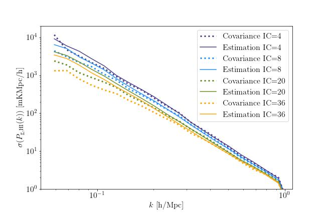
Figure 19: The comparison of the error bars coming from the estimate in Equation 9 versus the estimate from the covariance matrix of the GBT with the WiggleZ random catalogues.

References

- Ade et al. (2016) Ade P. A. R., et al., 2016, Astron. Astrophys., 594, A13
- Alam et al. (2021) Alam S., et al., 2021, Phys. Rev. D, 103, 083533
- Albareti et al. (2017) Albareti F. D., et al., 2017, Astrophys. J. Suppl., 233, 25
- Alonso et al. (2015) Alonso D., Bull P., Ferreira P. G., Santos M. G., 2015, Mon. Not. Roy. Astron. Soc., 447, 400
- Anderson et al. (2018) Anderson C. J., et al., 2018, Mon. Not. Roy. Astron. Soc., 476, 3382
- Ansari et al. (2012) Ansari R., et al., 2012, Astronomy & Astrophysics, 540, A129
- Asorey et al. (2020) Asorey J., et al., 2020, MNRAS, 495, 1788
- Bandura et al. (2014) Bandura K., et al., 2014, Proc. SPIE Int. Soc. Opt. Eng., 9145, 22
- Battye et al. (2004) Battye R. A., Davies R. D., Weller J., 2004, Mon. Not. Roy. Astron. Soc., 355, 1339
- Battye et al. (2013) Battye R. A., Browne I. W. A., Dickinson C., Heron G., Maffei B., Pourtsidou A., 2013, Mon. Not. Roy. Astron. Soc., 434, 1239
- Bautista et al. (2020) Bautista J. E., et al., 2020, Mon. Not. Roy. Astron. Soc., 500, 736
- Bera et al. (2019) Bera A., Kanekar N., Chengalur J. N., Bagla J. S., 2019, Astrophys. J. Lett., 882, L7
- Beutler et al. (2014) Beutler F., et al., 2014, Mon. Not. Roy. Astron. Soc., 443, 1065
- Blake (2019) Blake C., 2019, Mon. Not. Roy. Astron. Soc., 489, 153
- Blake et al. (2010) Blake C., et al., 2010, MNRAS, 406, 803
- Blake et al. (2011) Blake C., et al., 2011, MNRAS, 415, 2876
- Blanton et al. (2017) Blanton M. R., et al., 2017, AJ, 154, 28
- Bok et al. (2020) Bok J., Skelton R. E., Cluver M. E., Jarrett T. H., Jones M. G., Verdes-Montenegro L., 2020, arXiv.org, p. arXiv:2009.14585
- Braun (2012) Braun R., 2012, The Astrophysical Journal, 749, 87
- Bull et al. (2015) Bull P., Ferreira P. G., Patel P., Santos M. G., 2015, Astrophys. J., 803, 21
- Carucci et al. (2020) Carucci I. P., Irfan M. O., Bobin J., 2020, arXiv.org
- Castorina & White (2019) Castorina E., White M., 2019, JCAP, 06, 025
- Catinella et al. (2018) Catinella B., et al., 2018, Monthly Notices of the Royal Astronomical Society, 476, 875
- Chang et al. (2008) Chang T.-C., Pen U.-L., Peterson J. B., McDonald P., 2008, Physical Review Letters, 100
- Chang et al. (2010) Chang T.-C., Pen U.-L., Bandura K., Peterson J. B., 2010, Nature, 466, 463
- Chapman et al. (2012) Chapman E., et al., 2012, Mon. Not. Roy. Astron. Soc., 423, 2518
- Chen et al. (2019) Chen X., Wang J., Kong X., Catinella B., Shao L., Mo H., 2019, arXiv.org
- Chowdhury et al. (2020) Chowdhury A., Kanekar N., Chengalur J., Sethi S., Dwarakanath K. S., 2020, Nature, 586, 369
- Conroy & van Dokkum (2012) Conroy C., van Dokkum P. G., 2012, The Astrophysical Journal, 760, 71
- Cook et al. (2019) Cook R. H. W., Cortese L., Catinella B., Robotham A., 2019, Monthly Notices of the Royal Astronomical Society, 490, 4060
- Cortese et al. (2011) Cortese L., Catinella B., Boissier S., Boselli A., Heinis S., 2011, arXiv.org, pp 1797–1806
- Crighton et al. (2015) Crighton N. H., et al., 2015, Mon. Not. Roy. Astron. Soc., 452, 217
- Croton et al. (2006) Croton D. J., et al., 2006, Monthly Notices of the Royal Astronomical Society, 365, 11
- Cunnington et al. (2019) Cunnington S., Wolz L., Pourtsidou A., Bacon D., 2019, Mon. Not. Roy. Astron. Soc., 488, 5452
- Cunnington et al. (2020) Cunnington S., Pourtsidou A., Soares P. S., Blake C., Bacon D., 2020, Mon. Not. Roy. Astron. Soc., 496, 415
- Cunnington et al. (2021) Cunnington S., Irfan M. O., Carucci I. P., Pourtsidou A., Bobin J., 2021, Mon. Not. Roy. Astron. Soc., 504, 208
- Dawson et al. (2016) Dawson K. S., et al., 2016, Astron. J., 151, 44
- Dénes et al. (2014) Dénes H., Kilborn V. A., Koribalski B. S., 2014, Monthly Notices of the Royal Astronomical Society, 444, 667
- Drinkwater et al. (2010) Drinkwater M. J., et al., 2010, Monthly Notices of the Royal Astronomical Society, 401, 1429
- Gil-Marin et al. (2020) Gil-Marin H., et al., 2020, Mon. Not. Roy. Astron. Soc., 498, 2492
- Gunn et al. (2006) Gunn J. E., et al., 2006, AJ, 131, 2332
- Guo et al. (2020) Guo H., Jones M. G., Haynes M. P., Fu J., 2020, arXiv.org, p. 92
- Harper et al. (2018) Harper S. E., Dickinson C., Battye R. A., Roychowdhury S., Browne I. W. A., Ma Y. Z., Olivari L. C., Chen T., 2018, Monthly Notices of the Royal Astronomical Society, 478, 2416
- Hoppmann et al. (2015) Hoppmann L., Staveley-Smith L., Freudling W., Zwaan M. A., Minchin R. F., Calabretta M. R., 2015, A blind HI Mass Function from the Arecibo Ultra-Deep Survey (AUDS) (arXiv:1506.05931)
- Hothi et al. (2020) Hothi I., et al., 2020, Mon. Not. Roy. Astron. Soc., 500, 2264
- Hu et al. (2019) Hu W., et al., 2019, Mon. Not. Roy. Astron. Soc., 489, 1619
- Hu et al. (2020) Hu W., Wang X., Wu F., Wang Y., Zhang P., Chen X., 2020, Mon. Not. Roy. Astron. Soc., 493, 5854
- Hunter (2007) Hunter J. D., 2007, Computing In Science & Engineering, 9, 90
- Hyvärinen (1999) Hyvärinen A., 1999, IEEE transactions on neural networks, 10 3, 626
- Jones et al. (2001) Jones E., Oliphant T., Peterson P., et al., 2001, SciPy: Open source scientific tools for Python, http://www.scipy.org/
- Jones et al. (2018) Jones M. G., Haynes M. P., Giovanelli R., Moorman C., 2018, Monthly Notices of the Royal Astronomical Society, 477, 2–17
- Jones et al. (2020) Jones M. G., Hess K. M., Adams E. A. K., Verdes-Montenegro L., 2020, arXiv.org, pp 2090–2108
- Kaiser (1987) Kaiser N., 1987, Mon. Not. Roy. Astron. Soc., 227, 1
- Khandai et al. (2011) Khandai N., Sethi S. K., Di Matteo T., Croft R. A., Springel V., Jana A., Gardner J. P., 2011, Mon. Not. Roy. Astron. Soc., 415, 2580
- Lah et al. (2007) Lah P., et al., 2007, Mon. Not. Roy. Astron. Soc., 376, 1357
- Lang et al. (2016) Lang D., Hogg D. W., Schlegel D. J., 2016, AJ, 151, 36
- Lewis et al. (2000) Lewis A., Challinor A., Lasenby A., 2000, Astrophys. J., 538, 473
- Li et al. (2020a) Li Y., Santos M. G., Grainge K., Harper S., Wang J., 2020a, arXiv.org, p. arXiv:2007.01767
- Li et al. (2020b) Li J., et al., 2020b, Sci. China Phys. Mech. Astron., 63, 129862
- Liu & Tegmark (2011) Liu A., Tegmark M., 2011, Phys. Rev. D, 83, 103006
- Mao et al. (2008) Mao Y., Tegmark M., McQuinn M., Zaldarriaga M., Zahn O., 2008, Physical Review D, 78
- Marin et al. (2010) Marin F., Gnedin N. Y., Seo H.-J., Vallinotto A., 2010, Astrophys. J., 718, 972
- Martin et al. (2010) Martin A. M., Papastergis E., Giovanelli R., Haynes M. P., Springob C. M., Stierwalt S., 2010, Astrophys. J., 723, 1359
- Masui (2013) Masui K. W., 2013, PhD thesis, University of Toronto (Canada)
- Masui et al. (2010) Masui K. W., McDonald P., Pen U.-L., 2010, Phys. Rev. D, 81, 103527
- Masui et al. (2013) Masui K., et al., 2013, Astrophys. J., 763, L20
- Matteo et al. (2002) Matteo T. D., Perna R., Abel T., Rees M. J., 2002, The Astrophysical Journal, 564, 576
- McKinney (2010) McKinney W., 2010, in van der Walt S., Millman J., eds, Proceedings of the 9th Python in Science Conference. pp 51–56
- Murray (2018) Murray S. G., 2018, Journal of Open Source Software, 3, 850
- Neeleman et al. (2016) Neeleman M., Prochaska J. X., Ribaudo J., Lehner N., Howk J. C., Rafelski M., Kanekar N., 2016, Astrophys. J., 818, 113
- Newburgh et al. (2016) Newburgh L., et al., 2016, Proc. SPIE Int. Soc. Opt. Eng., 9906, 99065X
- Oh & Mack (2003) Oh S. P., Mack K. J., 2003, MNRAS, 346, 871
- Olivari et al. (2015) Olivari L. C., Remazeilles M., Dickinson C., 2015, arXiv.org
- Padmanabhan et al. (2016) Padmanabhan H., Choudhury T. R., Refregier A., 2016, Mon. Not. Roy. Astron. Soc., 458, 781
- Paul et al. (2017) Paul N., Choudhury T. R., Paranjape A., 2017, arXiv.org, pp 1627–1637
- Peterson et al. (2009) Peterson J. B., et al., 2009, 21 cm Intensity Mapping (arXiv:0902.3091)
- Pourtsidou et al. (2017) Pourtsidou A., Bacon D., Crittenden R., 2017, Mon. Not. Roy. Astron. Soc., 470, 4251
- Prakash et al. (2015) Prakash A., Licquia T. C., Newman J. A., Rao S. M., 2015, Astrophys. J., 803, 105
- Raichoor et al. (2020) Raichoor A., et al., 2020, Astron. Astrophys. Suppl. Ser., 4, 180
- Rao et al. (2006) Rao S. M., Turnshek D. A., Nestor D., 2006, Astrophys. J., 636, 610
- Rao et al. (2017) Rao S. M., Turnshek D. A., Sardane G. M., Monier E. M., 2017, Monthly Notices of the Royal Astronomical Society, 471, 3428–3442
- Reynolds et al. (2020) Reynolds T. N., Westmeier T., Staveley-Smith L., 2020, arXiv.org
- Rhee et al. (2013) Rhee J., Zwaan M. A., Briggs F. H., Chengalur J. N., Lah P., Oosterloo T., van der Hulst T., 2013, Mon. Not. Roy. Astron. Soc., 435, 2693
- Ross et al. (2020) Ross A. J., et al., 2020, Mon. Not. Roy. Astron. Soc., 498, 2354
- Rossi et al. (2021) Rossi G., et al., 2021, MNRAS, 505, 377
- SKA Cosmology SWG et al. (2020) SKA Cosmology SWG et al., 2020, Publ. Astron. Soc. Austral., 37, e007
- Santos et al. (2017) Santos M. G., et al., 2017, in MeerKAT Science: On the Pathway to the SKA. (arXiv:1709.06099)
- Seo et al. (2010) Seo H.-J., Dodelson S., Marriner J., Mcginnis D., Stebbins A., Stoughton C., Vallinotto A., 2010, The Astrophysical Journal, 721, 164
- Shaw et al. (2015) Shaw J. R., Sigurdson K., Sitwell M., Stebbins A., Pen U.-L., 2015, Phys. Rev. D, 91, 083514
- Smee et al. (2013) Smee S. A., et al., 2013, AJ, 146, 32
- Smith et al. (2003) Smith R., et al., 2003, Mon. Not. Roy. Astron. Soc., 341, 1311
- Soares et al. (2021) Soares P. S., Cunnington S., Pourtsidou A., Blake C., 2021, Mon. Not. Roy. Astron. Soc., 502, 2549
- Spinelli et al. (2020) Spinelli M., Zoldan A., De Lucia G., Xie L., Viel M., 2020, Monthly Notices of the Royal Astronomical Society, 493, 5434
- Spinelli et al. (2021) Spinelli M., Carucci I. P., Cunnington S., Harper S. E., Irfan M. O., Fonseca J., Pourtsidou A., Wolz L., 2021, SKAO HI Intensity Mapping: Blind Foreground Subtraction Challenge (arXiv:2107.10814)
- Springel et al. (2006) Springel V., Frenk C. S., White S. D. M., 2006, Nature, 440, 1137
- Stevens et al. (2016) Stevens A. R. H., Croton D. J., Mutch S. J., 2016, Monthly Notices of the Royal Astronomical Society, 461, 859
- Switzer et al. (2013) Switzer E. R., et al., 2013, Mon. Not. Roy. Astron. Soc.: Letters, 434, L46
- Switzer et al. (2015) Switzer E. R., Chang T.-C., Masui K. W., Pen U.-L., Voytek T. C., 2015, The Astrophysical Journal, 815, 51
- Takahashi et al. (2012) Takahashi R., Sato M., Nishimichi T., Taruya A., Oguri M., 2012, Astrophys. J., 761, 152
- Tamone et al. (2020) Tamone A., et al., 2020, Mon. Not. Roy. Astron. Soc., 499, 5527
- Villaescusa-Navarro et al. (2018) Villaescusa-Navarro F., et al., 2018, Astrophys. J., 866, 135
- Wang et al. (2021) Wang J., et al., 2021, Mon. Not. Roy. Astron. Soc., 505, 3698
- Wolz et al. (2014) Wolz L., Abdalla F., Blake C., Shaw J., Chapman E., Rawlings S., 2014, Mon. Not. Roy. Astron. Soc., 441, 3271
- Wolz et al. (2016a) Wolz L., Tonini C., Blake C., Wyithe J. S. B., 2016a, Monthly Notices of the Royal Astronomical Society, 458, 3399
- Wolz et al. (2016b) Wolz L., et al., 2016b, Mon. Not. Roy. Astron. Soc., 464, 4938
- Wolz et al. (2017) Wolz L., Blake C., Wyithe J. S. B., 2017, Monthly Notices of the Royal Astronomical Society, 470, 3220
- Wolz et al. (2019) Wolz L., Murray S. G., Blake C., Wyithe J. S., 2019, MNRAS, 484, 1007
- Wu et al. (2021) Wu F., et al., 2021, Mon. Not. Roy. Astron. Soc., 506, 3455
- Wyithe (2008) Wyithe S., 2008, Mon. Not. Roy. Astron. Soc., 388, 1889
- Wyithe & Loeb (2009) Wyithe J. S. B., Loeb A., 2009, Mon. Not. Roy. Astron. Soc., 397, 1926
- Zwaan et al. (2003) Zwaan M. A., et al., 2003, The Astronomical Journal, 125, 2842
- Zwaan et al. (2005) Zwaan M. A., Meyer M., Staveley-Smith L., Webster R., 2005, Mon. Not. Roy. Astron. Soc., 359, L30
- de Mattia et al. (2021) de Mattia A., et al., 2021, Mon. Not. Roy. Astron. Soc., 501, 5616
- van der Walt et al. (2011) van der Walt S., Colbert S. C., Varoquaux G., 2011, Computing in Science & Engineering, 13, 22