Constrained Secrecy Capacity of Finite-Input Intersymbol Interference Wiretap Channels

Abstract

We consider reliable and secure communication over intersymbol interference wiretap channels (ISI-WTCs). In particular, we first derive an achievable secure rate for ISI-WTCs without imposing any constraints on the input distribution. Afterwards, we focus on the setup where the input distribution of the ISI-WTC is constrained to be a time-invariant finite-order Markov chain. Optimizing the parameters of this Markov chain toward maximizing the achievable secure rates is a computationally intractable problem in general, and so, toward finding a local maximum, we propose an iterative algorithm that at every iteration replaces the secure rate function with a suitable surrogate function whose maximum can be found efficiently. Although the secure rates achieved in the unconstrained setup are potentially larger than the secure rates achieved in the constrained setup, the latter setup has the advantage of leading to efficient algorithms for estimating and optimizing the achievable secure rates, and also has the benefit of being the basis of efficient coding schemes.

I Introduction

I-A Motivation

The increasing number of connected users and the broadcasting nature of the wireless medium lead to a flurry of security challenges for wireless communication applications. For example, typical cryptographic protocols require significant communication resources for distributing and maintaining secret keys. This issue noticeably decreases the data transmission efficiency as the number of users gradually increases [2]. In addition, traditional cryptosystems rely on the assumption that eavesdroppers have limited computational power, making them vulnerable against more and more powerful (quantum) computers [3]. Alternatively, information-theoretic secrecy [4] utilizes the inherent randomness of communication channels to achieve security at the physical layer [5] without requiring secret key agreement and without imposing any constraints on the eavesdroppers’ computational power.

The emergence of different wireless applications gives rise to diverse channel models for various channel conditions. Intersymbol interference (ISI) channels are used as a model for high-data-rate transmission over wireless channels when the delay spread of the channel exceeds the symbol duration [6, Ch. 9]. In order to be specific, consider a multipath fading channel

$$Y(t_{\mathrm{c}})\triangleq\sum_{\ell=0}^{m_{\mathrm{c}}}g_{\mathrm{c},\ell}(t_{\mathrm{c}})X(t_{\mathrm{c}}-\tau_{\ell})+N(t_{\mathrm{c}}),$$

with continuous-time variable $t_{\mathrm{c}}\in\mathbb{R}$, where $X(t_{\mathrm{c}})$, $Y(t_{\mathrm{c}})$, and $N(t_{\mathrm{c}})$ denote the input, the output, and the additive noise signal, and where $g_{\mathrm{c},\ell}(t_{\mathrm{c}})$ and $\tau_{\ell}$ are, respectively, the gain and the delay of the $\ell$-th path, $0\leq\ell\leq m_{\mathrm{c}}$. When the symbol duration is smaller than $\tau_{\ell}-\tau_{0}$, the sampled output of a filter matched to the shaping pulse at the receiver leads to the ISI phenomenon. Such an ISI model usually appears in single-carrier communication systems, which require a higher power efficiency and a better peak-to-average power ratio (compared with multicarrier communication systems) and which appear in applications of the narrowband internet of things (NB-IoT) [8] as outlined in specifications of 5G and beyond-5G networks [9, 10]. Note that ISI is also caused by multipath propagation in long-range underwater acoustic communications [11], as well as in high data-rate ultra-wideband communication systems [12].

Providing security at the physical layer of the above-mentioned communication technologies without imposing extra delay, power consumption, and processing burden, has received significant attention recently [13, 14, 15]. In this paper, we mostly use scenarios from the NB-IoT technology for our examples and simulations. It is worthwhile to note that the NB-IoT mostly inherits the long-term evolution (LTE) infrastructure [9], so the essential channels operate in the licensed sub-GHz spectrum range [16]. In this spectrum range, in contrast to the broadcasting applications in the THz carrier frequency range [17], one cannot choose a sufficiently narrow angular divergence for the transmitter beam toward preventing the eavesdropper from intercepting non-line-of-sight transmission signals. This issue presents a vulnerable environment at the physical layer of applications using the NB-IoT.

These considerations motivate us to study theoretical aspects of the physical layer security over ISI wiretap channels (ISI-WTCs). As depicted in Fig. 1, the ISI-WTC comprises two ISI channels, where the primary channel connects a transmitter (called Alice) to a legitimate receiver (called Bob and abbreviated by “$\mathrm{B}$”), while the secondary channel connects the transmitter to an eavesdropper (called Eve and abbreviated by “$\mathrm{E}$”). In order to focus on the key aspects of this setup, the channel gains are assumed to be constant and perfectly known to the receiver over each transmission block.

Figure 1: Block diagram of the ISI-WTC.

I-B Background, Related Works, and Contributions

ISI channels with finite memory length and finite input alphabets are a particular case of finite-state machine channels (FSMCs) [19]. Toward maximizing the achievable information rates over FSMCs, the classical Blahut-Arimoto algorithm (BAA) [20, 21] was generalized in [22] to optimize finite-state machine sources (FSMSs) at the input of FSMCs. Comparing lower bounds on the capacity of FSMCs (i.e., the maximized information rates) [23, 22] with the corresponding upper bounds [24, 25] typically shows a small gap between them, which can be further narrowed by increasing the memory order of the FSMS at the input [26].

Recently, Han and Sasaki [27, 28] derived the secrecy capacity of memoryless wiretap channels with channel state information at the encoder. Dai et al. [29] applied these results to physically degraded Gaussian wiretap channels with noiseless private feedback from Bob’s observations to the encoder. It was shown in [29] that the considered feedback enhances the secrecy capacity under the weak secrecy criterion. The delayed version of this feedback is employed in [30] to enlarge the rate-equivocation region of finite-state Markov wiretap channels. Besides employing the feedback channel, the efficiency of secure communication over ISI channels can be enhanced by injecting cooperative artificial noise toward degrading Eve’s channel while minimizing the impact on Bob’s channel, as done in [31] and [32].

Due to power efficiency requirements, artificial-noise-aided communication has not received too much attention in recent technologies. Also, establishing a private noiseless channel to feed back the complete output of Bob’s channel to Alice’s encoder imposes a tremendous delay and processing overload on the higher layers of large cooperative networks. Hence, we focus on the standard version of ISI-WTCs (with neither feedback nor additional artificial noise), as it requires few assumptions and consequently is more practically relevant.

In terms of the main focus of this paper, estimating the secrecy capacity of a finite-state wiretap channel was already considered in [33]. However, the channel setup and the approach to estimate the secrecy capacity in [33] have the following limitations. Firstly, the assumptions for the channel setup in [33] resemble the general assumptions for memoryless wiretap channels as in [34], where Eve’s channel is assumed to be noisier than Bob’s channel. However, as we will show, these assumptions are inadequate for ISI channels (and more generally, for FSMCs) due to the non-flat frequency responses of these channels. Secondly, the gradient of the function that is used for approximating the secure rate function is usually not the same as the gradient of the secure rate function at a given operating point. This issue leads to an inaccurate search direction and eventually makes the algorithm unstable.

In the following, we highlight the main contributions and results presented in this paper.

• In the first step, we derive the achievable secure rates without imposing any constraints on the input distribution. We then focus on the setup where the input distribution is a time-invariant finite-order Markov chain, henceforth called an input Markov source. Note that employing Markov sources at the input of the ISI channels has the benefit of leading to efficient algorithms for estimation [36] and maximization [22] of information rates, approaching the capacity in point-to-point setups [26], and being a basis for efficient encoding and decoding schemes [37, 35]. Accordingly, we propose an efficient algorithm for optimizing the parameters of an input Markov source toward maximizing the obtained achievable secure rates over ISI-WTCs.

• Maximizing the above-mentioned secure rate is challenging because it is not a closed-form function of the input distribution and its evaluation is only possible through Monte-Carlo simulations. The key idea behind the proposed algorithm is to iteratively approximate the zeroth-order and the first-order behavior of the secure rate function by suitable surrogate functions that are well-defined and can relatively easily be maximized.

• We provide examples where the capacity of Eve’s channel is higher than the capacity of Bob’s channel, yet a nonzero secure rate is possible. These examples show that it is feasible to optimize an input Markov source such that spectral discrepancies between the frequency responses of Bob’s and Eve’s channels can be exploited—without any further power consumption for transmitting interfering artificial noise toward jamming Eve’s channel.

I-C Paper Organization

The remainder of this paper is organized as follows. Section II introduces the system model and some preliminary concepts related to FSMCs, ISI-WTCs, and achievable secure rates. Section III describes the proposed algorithm for optimizing the parameters of a Markov source at the input of an ISI-WTC and analyzes it in detail. Section IV contains some numerical results and discussions. Finally, Section V draws the conclusions.

I-D Notation

The sets of integers and complex numbers are denoted by $\mathbb{Z}$ and $\mathbb{C}$, respectively. The ring of polynomials with coefficients in $\mathbb{C}$ and indeterminate $D$ is denoted by $\mathbb{C}[D]$, where “$D$” stands for “delay”. Other than that, sets are denoted by calligraphic letters, e.g., $\mathcal{S}$. The Cartesian product of two sets $\mathcal{X}$ and $\mathcal{Y}$ is written as $\mathcal{X}\times\mathcal{Y}$, and the $n$-fold Cartesian product of $\mathcal{X}$ with itself is written as $\mathcal{X}^{n}$. If $\mathcal{X}$ is a finite set, then its cardinality is denoted by $|\mathcal{X}|$.

Random variables are denoted by upper-case italic letters, e.g., $X$, their realizations by the corresponding lower-case letters, e.g., $x$, and the set of possible values by the corresponding calligraphic letter, e.g., $\mathcal{X}$. Random vectors are denoted by upper-case boldface letters, e.g., $\mathbf{X}$, and their realizations by the corresponding lower-case letters, e.g., $\mathbf{x}$. For integers $n_{1}$ and $n_{2}$ satisfying $n_{1}<n_{2}$, the notation $\mathbf{X}_{n_{1}}^{n_{2}}\triangleq(X_{n_{1}},X_{n_{1}+1},\ldots,X_{n_{2}})$ is used for a time-indexed vector of random variables and $\mathbf{x}_{n_{1}}^{n_{2}}\triangleq(x_{n_{1}},x_{n_{1}+1},\ldots,x_{n_{2}})$ for its realization. Boldface letters are also used for matrices, e.g., $\mathbf{A}$, with the $(i,j)$-entry of $\mathbf{A}$ being called $A_{ij}$.

For any real number $x$, the expression $(x)^{+}$ stands for $\max\{x,0\}$; similarly, $f^{+}(\cdot)$ stands for $\big{(}f(\cdot)\big{)}^{+}$. Moreover, the expression $\log(\,\cdot\,)$ denotes the natural logarithm function.

The entropy of a random variable $X$, the mutual information between two random variables $X$ and $Y$, and the mutual information between two random variables $X$ and $Y$ conditioned on the random variable $Z$ are denoted by $H(X)$, $I(X;Y)$, and $I(X;Y|Z)$, respectively. Finally, the variational distance between the probability mass functions (PMFs) of two random variables $X$ and $Y$ over the same finite alphabet $\mathcal{X}$ is defined as

$$d_{\mathcal{X}}(p_{X},p_{Y})\triangleq\sum\limits_{x\in\mathcal{X}}\ \bigl{|}p_{X}(x)-p_{Y}(x)\bigr{|}.$$

II Preliminaries

II-A Channel Model

An ISI channel with transfer polynomial $g(D)\triangleq\sum_{t=0}^{m}g_{t}D^{t}\in\mathbb{C}[D]$, where $g_{m}\neq 0$ and where $m$ is called the memory length, has an input process $\{X_{t}\}_{t\in\mathbb{Z}}$, a noiseless output process $\{U_{t}\}_{t\in\mathbb{Z}}$, a noise process $\{N_{t}\}_{t\in\mathbb{Z}}$, and a noisy output process $\{Y_{t}\}_{t\in\mathbb{Z}}$ with

$$U_{t} \triangleq\sum_{\ell=0}^{m}g_{\ell}X_{t-\ell}, \quad t\in\mathbb{Z},$$

$$Y_{t} \triangleq U_{t}+N_{t}, \quad t\in\mathbb{Z},$$

where $X_{t},U_{t},{N_{t},\,}Y_{t}\in\mathbb{C}$ for all $t\in\mathbb{Z}$, and where the noise process is independent of the channel input process. In the following, we will assume that the noise process is white Gaussian noise, i.e., $\{N_{t}\}_{t\in\mathbb{Z}}$ are i.i.d. Gaussian random variables with mean zero and variance $\sigma^{2}$. Clearly, an ISI channel is parameterized by the couple $\bigl{(}g(D),\sigma^{2}\bigr{)}$.

An ISI channel described by $\bigl{(}g(D)\triangleq\sum_{t=0}^{m}g_{t}D^{t},\ \sigma^{2}\bigr{)}$, where $m<\infty$, and having an input process $\{X_{t}\}_{t\in\mathbb{Z}}$ taking values in a finite set $\mathcal{X}\subsetneq\mathbb{C}$ is a special case of the channels in the class of finite-state machine channels (FSMCs), which were called finite-state channels in [19]. Indeed, let $s_{t}\triangleq\mathbf{x}_{t-\nu+1}^{t}$ (with $\mathcal{S}\triangleq\mathcal{X}^{\nu}$ and $\nu\geq m$) denote the state of an FSMC modeling an ISI channel at $t\in\mathbb{Z}$. Then

$$p_{S_{t},Y_{t}|S_{t-1},X_{t}}(s_{t},y_{t}|s_{t-1},x_{t})$$

$$\quad\quad=p_{S_{t}|S_{t-1},X_{t}}(s_{t}|s_{t-1},x_{t})\cdot p_{Y_{t}|S_{t-1},X_{t}}(y_{t}|s_{t-1},x_{t}),$$

where

$$p_{S_{t}|S_{t-1},X_{t}}(s_{t}|s_{t-1},x_{t}) \triangleq\begin{cases}\begin{array}[]{l}1\mbox{}\end{array}&\begin{array}[]{l}\text{(if $s_{t}=\mathbf{x}_{t-\nu+1}^{t},s_{t-1}=\mathbf{x}_{t-\nu}^{t-1})$}\end{array}\\ \\ \begin{array}[]{l}0\end{array}&\begin{array}[]{l}\text{(otherwise)}\end{array}\end{cases},$$

$$p_{Y_{t}|S_{t-1},X_{t}}(y_{t}|s_{t-1},x_{t}) \triangleq\frac{1}{{2\pi\sigma^{2}}}\cdot\exp\left(-\frac{|y_{t}-u_{t}|^{2}}{2\sigma^{2}}\right),$$

with $s_{t-1}=\mathbf{x}_{t-\nu}^{t-1}(\in\mathcal{X}^{\nu})$ and $u_{t}=\sum_{\ell=0}^{m}g_{\ell}x_{t-\ell}$.

All possible state sequences of an ISI channel (and more generally, of an FSMC) can be represented by a trellis diagram. Because of the assumed time invariance, it is sufficient to show a single trellis section. For example, Fig. 2($a$) shows a trellis section of an ISI channel characterized by the couple $\bigl{(}g(D)\triangleq 1-D,\ \sigma^{2}\bigr{)}$ with $\nu=1$ and input alphabet $\mathcal{X}\triangleq\{+1,-1\}$. In this diagram, branches start at state $s_{t-1}\,\triangleq\,x_{t-1}$, end at state $s_{t}\,\triangleq\,\,x_{t}$, and have noiseless channel output symbol $u_{t}=x_{t}-x_{t-1}$ shown next to them.

Figure 2: ($a$) Trellis section of an FSMC, modeling an ISI channel with $g(D)=1-D$, when used with $\nu=1$ and $\mathcal{X}=\{+1,-1\}$. The noiseless channel output symbol $u_{t}$ is shown next to the branches. ($b$) Trellis section of an FSMC, modeling an ISI-WTC with $g^{\mathrm{B}}(D)=1-D$ and $g^{\mathrm{E}}(D)=1+D-D^{2}-D^{3}$, when used with $\nu=3$ and $\mathcal{X}=\{+1,-1\}$. Noiseless channel output symbols $(u_{t},v_{t})$, one noiseless channel output symbol for Bob’s channel and one noiseless channel output symbol for Eve’s channel, are shown next to the branches.

Let $\mathcal{B}$ $(\subseteq\mathcal{S}\times\mathcal{S})$ denote the set of all valid consecutive state pairs $(s_{t-1},s_{t})$ for which $p_{S_{t}|S_{t-1}}(s_{t}|s_{t-1})$ is allowed to be non-zero for any $t\in\mathbb{Z}$. Moreover, let

$$\overrightarrow{\mathcal{S}}_{\!i}\triangleq\bigl{\{}j\bigm{|}(i,j)\in\mathcal{B}\bigr{\}},\quad\overleftarrow{\mathcal{S}}_{\!j}\triangleq\bigl{\{}i\bigm{|}(i,j)\in\mathcal{B}\bigr{\}},$$

be the set of states $S_{t}\in\mathcal{S}$ reachable from $S_{t-1}=i$ and the set of states $S_{t-1}\in\mathcal{S}$ that can reach $S_{t}=j$, respectively. For every $(i,j)\in\mathcal{B}$, let $p_{ij}\triangleq p_{S_{t}|S_{t-1}}(j|i)$ be the time-invariant state transition probability assigned by an ergodic and non-periodic Markov source of memory order $\nu$. Then there is a unique stationary state PMF $\{\mu_{i}\}_{i\in\mathcal{S}}$ such that $p_{S_{t}}(i)=\mu_{i}$ for all $t\in\mathbb{Z}$, $i\in\mathcal{S}$. Finally, let $Q_{ij}\triangleq\mu_{i}\cdot p_{ij}$, for all $(i,j)\in\mathcal{B}$.

In the above statements, we started with $\{p_{ij}\}_{(i,j)\in\mathcal{B}}$ and derived $\{\mu_{i}\}_{i\in\mathcal{S}}$ and $\{Q_{ij}\}_{(i,j)\in\mathcal{B}}$ from $\{p_{ij}\}_{(i,j)\in\mathcal{B}}$. However, for analytical purposes, it turns out to be beneficial to start with $\{Q_{ij}\}_{(i,j)\in\mathcal{B}}$ and derive $\{p_{ij}\}_{(i,j)\in\mathcal{B}}$ and $\{\mu_{i}\}_{i\in\mathcal{S}}$ from $\{Q_{ij}\}_{(i,j)\in\mathcal{B}}$. Note that the set of all valid $\{Q_{ij}\}_{(i,j)\in\mathcal{B}}$ for a fixed set $\mathcal{B}$ is given by the polytope $\mathcal{Q}(\mathcal{B})$, where

$$\mathcal{Q}(\mathcal{B}) \triangleq\left\{\{Q_{ij}\}_{(i,j)\in\mathcal{B}}\ \middle|\begin{array}[]{r@{\ }c@{\ }l}Q_{ij}&\geq&0,\ \forall(i,j)\in\mathcal{B},\\ \sum\limits_{(i,j)\in\mathcal{B}}Q_{ij}&=&1,\\ \sum\limits_{j\in\overrightarrow{\mathcal{S}}_{\!i}}Q_{ij}&=&\sum\limits_{k\in\overleftarrow{\mathcal{S}}_{\!i}}Q_{ki},\ \forall i\in\mathcal{S}\!\end{array}\!\!\right\}\!.$$

(See [22] for similar observations.) In the following, we will use the short-hand notation $\mathbf{Q}$ for $\{Q_{ij}\}_{(i,j)\in\mathcal{B}}$. Moreover, similar to [22, Assumption 34], we will only be interested in sets $\mathcal{B}$ where the Markov sources corresponding to relative interior points of $\mathcal{Q}(\mathcal{B})$ are ergodic and non-periodic.

Remark 1 (Parameterized family of $\mathbf{Q}$).

Frequently, we will consider the setup where $\mathbf{Q}$ is a function of some parameter $\theta$. More precisely, for every $(i,j)\in\mathcal{B}$, we let $Q_{ij}(\theta)$ be a smooth function of the parameter $\theta$, where $\theta$ varies over a suitable range. For every $\theta$, we require that $\mathbf{Q}(\theta)\triangleq\bigl{\{}Q_{ij}(\theta)\bigr{\}}_{(i,j)\in\mathcal{B}}\in\mathcal{Q}(\mathcal{B})$. Moreover, for every $(i,j)\in\mathcal{B}$, we denote the derivative of $Q_{ij}(\theta)$ w.r.t. $\theta$ and evaluated at $\tilde{\theta}$ by $Q^{\theta}_{ij}(\tilde{\theta})$. We denote the corresponding steady-state and state transition probabilities parameterized by $\theta$ by $\mu_{i}(\theta)$ and $p_{ij}(\theta)$, respectively. Similarly, we denote their derivatives w.r.t. $\theta$ and evaluated at $\tilde{\theta}$ by $\mu_{i}^{\theta}(\tilde{\theta})$ and $p_{ij}^{\theta}(\tilde{\theta})$, respectively. Because $\mathbf{Q}(\theta)\in\mathcal{Q}(\mathcal{B})$, we have $\sum_{(i,j)\in\mathcal{B}}Q^{\theta}_{ij}(\tilde{\theta})=0,$ and $\sum_{i\in{\mathcal{S}}}\mu_{i}^{\theta}(\tilde{\theta})=0$. $\square$

Definition 1 (Intersymbol Interference Wiretap Channel (ISI-WTC)).

In this paper, we consider an ISI-WTC, where Alice transmits data symbols over Bob’s channel and over Eve’s channel, which are both assumed to be ISI channels with finite input alphabet $\mathcal{X}\subsetneq\mathbb{C}$. (See Fig. 1.) Specifically, Bob’s channel is an ISI channel described by the couple $\bigl{(}g^{\mathrm{B}}(D),\sigma_{\mathrm{B}}^{2}\bigr{)}$, with transfer polynomial $g^{\mathrm{B}}(D)=\sum_{t=0}^{m_{\mathrm{B}}}g^{\mathrm{B}}_{t}D^{t}$, noiseless output process $\{U_{t}\}_{t\in\mathbb{Z}}$, noise process $\{N^{\mathrm{B}}_{t}\}_{t\in\mathbb{Z}}$, and noisy output process $\{Y_{t}\}_{t\in\mathbb{Z}}$. Similarly, Eve’s channel is an ISI channel described by the couple $\bigl{(}g^{\mathrm{E}}(D),\sigma_{\mathrm{E}}^{2}\bigr{)}$, with transfer polynomial $g^{\mathrm{E}}(D)=\sum_{t=0}^{m_{\mathrm{E}}}g^{\mathrm{E}}_{t}D^{t}$, noiseless output process $\{V_{t}\}_{t\in\mathbb{Z}}$, noise process $\{N^{\mathrm{E}}_{t}\}_{t\in\mathbb{Z}}$, and noisy output process $\{Z_{t}\}_{t\in\mathbb{Z}}$. We assume that the noise process of Bob’s channel and the noise process of Eve’s channel are independent. Clearly, the ISI-WTC is parameterized by the quadruple $\bigl{(}g^{\mathrm{B}}(D),g^{\mathrm{E}}(D),\sigma_{\mathrm{B}}^{2},\sigma_{\mathrm{E}}^{2}\bigr{)}$. $\square$

By choosing $\nu\geq\max(m_{\mathrm{B}},m_{\mathrm{E}})$, FSMCs and their associated trellises can be used for visualizing ISI-WTCs as well. Since such trellis representations are well known, we omit the details and conclude this section with the following example. (See [1] and [33] for more details.)

Consider an ISI-WTC with $\mathcal{X}=\{+1,-1\}$, where Bob’s channel is described by $g^{\mathrm{B}}(D)=1-D$ (see Fig. 2($a$)), and where Eve’s channel is described by $g^{\mathrm{E}}(D)=1+D-D^{2}-D^{3}$. Let $\nu=3$. Then all possible state sequences of an FSMC modeling this ISI-WTC can be represented by a trellis diagram. Because of the assumed time invariance, it is sufficient to show a single trellis section, as shown in Fig. 2($b$) for the present example.

II-B Secure Rate

Definition 2.

An $\bigl{(}{e^{nR_{\mathrm{s}}}},n\bigr{)}$ code for the wiretap channel consists of a message set $\mathcal{M}$ with $|\mathcal{M}|\triangleq\big{\lceil}e^{nR_{\mathrm{s}}}\big{\rceil}$, a stochastic encoder $f:\mathcal{M}\to\mathcal{X}^{n}$, and a decoder $\phi:\mathbb{C}^{n}\to\mathcal{M}$. $\square$

Let $M$ be a random variable corresponding to a uniformly chosen secret message from the alphabet $\mathcal{M}$. The reliability of Bob’s decoder is measured by the probability of a block error $\Pr\big{(}M\neq\phi(\mathbf{Y}^{n})\big{)}$ and the secrecy performance of the code is measured by the statistical independence between $M$ and $\mathbf{Z}_{1}^{n}$ in terms of the variational distance $d_{\mathcal{M}\times\mathcal{Z}^{n}}(p_{M,\mathbf{Z}_{1}^{n}},p_{M}p_{\mathbf{Z}_{1}^{n}})$. (See Appendix A for more details.)

Definition 3.

A secure rate $R_{\mathrm{s}}$ is said to be achievable if there exists a sequence of codes $\bigl{(}{e^{nR_{\mathrm{s}}}},n\bigr{)}$ as in Definition 2, with $n\to\infty$, satisfying the reliability criterion

$$\Pr\big{(}M\neq\phi(\mathbf{Y}^{n})\big{)}\rightarrow 0,$$ (1)

and the secrecy criterion

$$d_{\mathcal{M}\times\mathcal{Z}^{n}}(p_{M,\mathbf{Z}_{1}^{n}},p_{M}p_{\mathbf{Z}_{1}^{n}})\rightarrow 0.$$ (2)

The secrecy capacity is the supremum of all achievable secure rates. $\square$

Definition 4.

Consider an ISI-WTC with an input Markov source described by $\mathbf{Q}\in\mathcal{Q}(\mathcal{B})$. For all $(i,j)\in\mathcal{B}$, define $T^{\mathrm{B}}_{ij}(\mathbf{Q})$ and $T^{\mathrm{E}}_{ij}(\mathbf{Q})$ as shown in (3) and (4) at the bottom of this page. $\square$

$$\!\!T^{\mathrm{B}}_{ij}(\mathbf{Q}) \triangleq\lim_{n\to\infty}\int p_{\mathbf{Y}_{1}^{n}}(\mathbf{y}_{1}^{n})\cdot\check{T}^{\mathrm{B}}_{ij}(\mathbf{Q},\mathbf{y}_{1}^{n})\ \mathrm{d}{\mathbf{y}_{1}^{n}},\ \ \check{T}^{\mathrm{B}}_{ij}(\mathbf{Q},\mathbf{y}_{1}^{n}) \triangleq\frac{1}{n}\sum_{t=1}^{n}\log\left(\frac{p_{S_{t-1},S_{t}|\mathbf{Y}_{1}^{n}}(i,j|\mathbf{y}_{1}^{n})^{{p_{S_{t-1},S_{t}|\mathbf{Y}_{1}^{n}}(i,j|\mathbf{y}_{1}^{n})}/{\mu_{i}p_{ij}}}}{p_{S_{t-1}|\mathbf{Y}_{1}^{n}}(i|\mathbf{y}_{1}^{n})^{{p_{S_{t-1}|\mathbf{Y}_{1}^{n}}(i|\mathbf{y}_{1}^{n})}/{\mu_{i}}}}\right)\!,\!$$ (3)

$$\!\!T^{\mathrm{E}}_{ij}(\mathbf{Q}) \triangleq\lim_{n\to\infty}\int p_{\mathbf{Z}_{1}^{n}}(\mathbf{z}_{1}^{n})\cdot\check{T}^{\mathrm{E}}_{ij}(\mathbf{Q},\mathbf{z}_{1}^{n})\ \mathrm{d}{\mathbf{z}_{1}^{n}},\ \ \check{T}^{\mathrm{E}}_{ij}(\mathbf{Q},\mathbf{z}_{1}^{n}) \triangleq\frac{1}{n}\sum_{t=1}^{n}\log\left(\frac{p_{S_{t-1},S_{t}|\mathbf{Z}_{1}^{n}}(i,j|\mathbf{z}_{1}^{n})^{{p_{S_{t-1},S_{t}|\mathbf{Z}_{1}^{n}}(i,j|\mathbf{z}_{1}^{n})}/{\mu_{i}p_{ij}}}}{p_{S_{t-1}|\mathbf{Z}_{1}^{n}}(i|\mathbf{z}_{1}^{n})^{{p_{S_{t-1}|\mathbf{Z}_{1}^{n}}(i|\mathbf{z}_{1}^{n})}/{\mu_{i}}}}\right)\!,\!$$ (4)

$$\bar{\psi}_{\tilde{\mathbf{Q}}}(\mathbf{Q}) \triangleq\kappa^{\prime}\cdot\Bigg{(}\sum_{(i,j)\in\mathcal{B}}\tilde{Q}_{ij}\cdot\bigl{(}1+\kappa\cdot(\delta Q)_{ij}\bigr{)}\ \cdot \log\bigl{(}1+ \kappa\cdot(\delta Q)_{ij}\big{)}-\sum_{i\in\mathcal{S}}\tilde{\mu}_{i}\cdot\bigl{(}1+\kappa\cdot(\delta\mu)_{i}\bigr{)}\cdot\log\bigl{(}1+\kappa\cdot(\delta\mu)_{i}\bigl{)}\Bigg{)}.$$ (5)

Proposition 1.

Consider an ISI-WTC with an input Markov source described by $\mathbf{Q}\in\mathcal{Q}(\mathcal{B})$. Let

$$R_{\mathrm{s}}(\mathbf{Q})\triangleq\bigg{(}\sum_{(i,j)\in\mathcal{B}}Q_{ij}\cdot\bigl{(}T^{\mathrm{B}}_{ij}(\mathbf{Q})-T^{\mathrm{E}}_{ij}(\mathbf{Q})\bigr{)}\bigg{)}^{\!\!+}.$$ (6)

Then all secure rates $R_{\mathrm{s}}$ satisfying

$$R_{s}<R_{\mathrm{s}}(\mathbf{Q})$$

are achievable over this ISI-WTC under the reliability criterion (1) and the secrecy criterion (2).

Proof.

See Appendix B. ∎

The expressions in (3) and (4) make it appear very unlikely that there is a closed-form expression for $R_{\mathrm{s}}(\mathbf{Q})$ in terms of $\mathbf{Q}$. Accordingly, the best one can do is to estimate $R_{\mathrm{s}}(\mathbf{Q})$ for a specific $\mathbf{Q}\in\mathcal{Q}(\mathcal{B})$ through Monte-Carlo methods (e.g., variants of the algorithms in [36]).

We are now in a position to introduce the notion of constrained secrecy capacity, which is a key quantity to be studied in the subsequent parts of this paper.

Definition 5.

Consider an ISI-WTC with an input Markov source described by $\mathbf{Q}$, varying over $\mathcal{Q}(\mathcal{B})$. The constrained secrecy capacity (or, more precisely, the $\mathcal{Q}(\mathcal{B})$-constrained secrecy capacity) is defined as

$$C_{\mathcal{Q}(\mathcal{B})}\triangleq\max_{\mathbf{Q}\in\mathcal{Q}(\mathcal{B})}R_{\mathrm{s}}(\mathbf{Q}).$$

$\square$

Roughly speaking, $C_{\mathcal{Q}(\mathcal{B})}$ is the tightest lower bound on the secrecy capacity of an ISI-WTC that can be obtained by optimizing an input Markov source described by $\mathbf{Q}\in\mathcal{Q}(\mathcal{B})$.

The next section (Section III) discusses an efficient algorithm for finding a local maximum of $R_{\mathrm{s}}(\mathbf{Q})$ over $\mathcal{Q}(\mathcal{B})$. In a first reading of this paper, readers might want to skip this (rather technical) section and go straight to Section IV that discusses some simulation results.

III Secure Rate Optimization

A first challenge when optimizing the function $R_{\mathrm{s}}(\mathbf{Q})$ over $\mathcal{Q}(\mathcal{B})$ is the fact that we do not have a closed-form expression for $R_{\mathrm{s}}(\mathbf{Q})$, i.e., the best we can do is to approximate $R_{\mathrm{s}}(\mathbf{Q})$ by estimating it with the help of Monte-Carlo methods. However, instead of applying a standard zeroth-order optimization method that is based on estimates of $R_{\mathrm{s}}(\mathbf{Q})$, in this section we pursue a more efficient approach that is based on estimates of the gradient of $R_{\mathrm{s}}(\mathbf{Q})$.

A second challenge when optimizing the function $R_{\mathrm{s}}(\mathbf{Q})$ over $\mathcal{Q}(\mathcal{B})$ is the fact that $R_{\mathrm{s}}(\mathbf{Q})$ is (typically, according to our numerical investigations in Section IV) a fluctuating, non-concave function. Therefore, we will aim at finding a local maximum of $R_{\mathrm{s}}(\mathbf{Q})$ instead of the global maximum. (Of course, by running the optimization algorithm with different initializations, one can potentially get different local maxima. Finally, the maximum among all local maxima is then selected. See also the discussion in Section IV.)

Our iterative optimization method operates as follows:

• Assume that at the current iteration the algorithm has found a Markov source described by $\tilde{\mathbf{Q}}\triangleq\bigl{\{}\tilde{Q}_{ij}\bigr{\}}_{(i,j)\in\mathcal{B}}$.

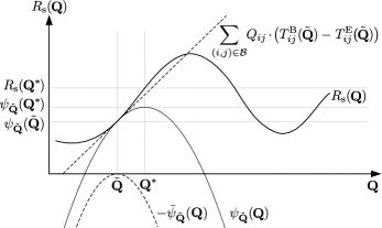
• Around $\mathbf{Q}=\tilde{\mathbf{Q}}$, the algorithm approximates the secure rate function $R_{\mathrm{s}}(\mathbf{Q})$ by the surrogate function $\psi_{\tilde{\mathbf{Q}}}(\mathbf{Q})$ over $\mathcal{Q}(\mathcal{B})$ satisfying the following properties:

  • The value of $\psi_{\tilde{\mathbf{Q}}}(\mathbf{Q})$ matches the value of $R_{\mathrm{s}}(\mathbf{Q})$ at $\mathbf{Q}=\tilde{\mathbf{Q}}$.

  • The gradient of $\psi_{\tilde{\mathbf{Q}}}(\mathbf{Q})$ w.r.t. $\mathbf{Q}$ matches the gradient of $R_{\mathrm{s}}(\mathbf{Q})$ w.r.t. $\mathbf{Q}$ at $\mathbf{Q}=\tilde{\mathbf{Q}}$.

  • The function $\psi_{\tilde{\mathbf{Q}}}(\mathbf{Q})$ is concave in terms of $\mathbf{Q}$ and can be efficiently maximized.

• Replace $\tilde{\mathbf{Q}}$ with the $\mathbf{Q}$ maximizing $\psi_{\tilde{\mathbf{Q}}}(\mathbf{Q})$.

As sketched in Fig. 3, a well-defined concave surrogate function with the mentioned properties enables us to search throughout the polytope $\mathcal{Q}(\mathcal{B})$ and find a local maximum of $R_{\mathrm{s}}(\mathbf{Q})$ over $\mathcal{Q}(\mathcal{B})$, iteratively. Similar techniques have also been proposed in [22, 38].

Figure 3: Sketch of the functions appearing in the optimization algorithm discussed in Section III. Note that while the domain is one-dimensional in this sketch, it is $|\mathcal{B}|$-dimensional in the actual optimization problem.

III-A The Surrogate Function

In this section, we first introduce the surrogate function. Then, we show that the employed surrogate function fulfills the promised properties.

In the following, in the same way that we derived $\{p_{ij}\}_{(i,j)\in\mathcal{B}}$ and $\{\mu_{i}\}_{i\in\mathcal{S}}$ from $\mathbf{Q}=\{Q_{ij}\}_{(i,j)\in\mathcal{B}}$ , we will derive $\{\tilde{p}_{ij}\}_{(i,j)\in\mathcal{B}}$ and $\{\tilde{\mu}_{i}\}_{i\in\mathcal{S}}$ from $\tilde{\mathbf{Q}}=\{\tilde{Q}_{ij}\}_{(i,j)\in\mathcal{B}}$. For every $(i,j)\in\mathcal{B}$, let

$$(\delta Q)_{ij}\triangleq\frac{Q_{ij}-\tilde{Q}_{ij}}{\tilde{Q}_{ij}},\ (\delta\mu)_{i}\triangleq\frac{\mu_{i}-\tilde{\mu}_{i}}{\tilde{\mu}_{i}}.$$

Moreover, let $\bar{\psi}_{\tilde{\mathbf{Q}}}(\mathbf{Q})$ be as defined in (5), shown at the bottom of the previous page, where the real parameters $0<\kappa\leq 1$ and $\kappa^{\prime}>0$ are used to control the shape of $\bar{\psi}_{\tilde{\mathbf{Q}}}(\mathbf{Q})$. For a given operating point $\tilde{\mathbf{Q}}\in\mathcal{Q}(\mathcal{B})$, the surrogate function is specified by (see also Fig. 3)

$$\psi_{\tilde{\mathbf{Q}}}(\mathbf{Q}) \triangleq\underbrace{\sum_{(i,j)\in\mathcal{B}}Q_{ij}\cdot\bigl{(}T^{\mathrm{B}}_{ij}(\tilde{\mathbf{Q}})-T^{\mathrm{E}}_{ij}(\tilde{\mathbf{Q}})\bigr{)}}_{\text{\char 172}}\underbrace{-\ {\bar{\psi}_{\tilde{\mathbf{Q}}}(\mathbf{Q})}_{\parbox{2.84544pt}{\mbox{} \\ }}\!.}_{\text{\char 173}}$$ (7)

Note that, for a fixed $\tilde{\mathbf{Q}}$, the expression ① is linear in $\mathbf{Q}$, while the expression ② is concave in $\mathbf{Q}$ and has a zero gradient for $\mathbf{Q}=\tilde{\mathbf{Q}}$. The role of the expression ① is to be a first-order approximation of $R_{\mathrm{s}}(\mathbf{Q})$ at $\mathbf{Q}=\tilde{\mathbf{Q}}$, while the role of ② is to regularize $\psi_{\tilde{\mathbf{Q}}}(\mathbf{Q})$. While many other expressions than ② could have been chosen as a regularization term, the expression in ② yields the following desirable features for $\psi_{\tilde{\mathbf{Q}}}(\mathbf{Q})$: first, the function $\psi_{\tilde{\mathbf{Q}}}(\mathbf{Q})$ can be efficiently maximized over $\mathbf{Q}$, second, maximizing $\psi_{\tilde{\mathbf{Q}}}(\mathbf{Q})$ implicitly also improves the entropy rate of the input Markov source described by $\mathbf{Q}$.

In the following, we examine the promised properties of the employed surrogate function (7). For brevity, we use the short-hand notations $R_{\mathrm{s}}(\theta)$, $\psi_{\tilde{\mathbf{Q}}}(\theta)$, and $\tilde{\mathbf{Q}}$ for $R_{\mathrm{s}}\bigl{(}\mathbf{Q}(\theta)\bigr{)}$, $\psi_{\tilde{\mathbf{Q}}}\bigl{(}\mathbf{Q}(\theta)\bigr{)}$, and $\mathbf{Q}(\tilde{\theta})\in\mathcal{Q}(\mathcal{B})$, respectively.

Lemma 1 (Property 1 of the surrogate function $\psi$).

The value of $\psi_{\tilde{\mathbf{Q}}}(\mathbf{Q})$ matches the value of $R_{\mathrm{s}}(\mathbf{Q})$ at $\mathbf{Q}=\tilde{\mathbf{Q}}$, i.e., $\psi_{\tilde{\mathbf{Q}}}(\tilde{\mathbf{Q}})=R_{\mathrm{s}}(\tilde{\mathbf{Q}}),$ and, in terms of the parameterization defined above, $\psi_{\tilde{\mathbf{Q}}}(\tilde{\theta})=R_{\mathrm{s}}(\tilde{\theta}).$

Proof.

We start by noting that $\mathbf{Q}=\tilde{\mathbf{Q}}$ implies $(\delta Q)_{ij}=0$ and $(\delta\mu)_{i}=0$ for all $(i,j)\in\mathcal{B}$, which in turn implies that $\bar{\psi}_{\tilde{\mathbf{Q}}}(\tilde{\mathbf{Q}})=0$. The result $\psi_{\tilde{\mathbf{Q}}}(\tilde{\mathbf{Q}})=R_{\mathrm{s}}(\tilde{\mathbf{Q}})$ follows then from (7) along with (6) in Proposition 1. ∎

Lemma 2 (Property 2 of the surrogate function $\psi$).

The gradient of $\psi_{\tilde{\mathbf{Q}}}(\mathbf{Q})$ w.r.t. $\mathbf{Q}$ matches the gradient of $R_{\mathrm{s}}(\mathbf{Q})$ w.r.t. $\mathbf{Q}$ at $\mathbf{Q}=\tilde{\mathbf{Q}}$, i.e.,

$$\left.\frac{\operatorname{d}}{\operatorname{d}\hskip-0.99594pt\theta}\psi_{\tilde{\mathbf{Q}}}(\theta)\right|_{\theta=\tilde{\theta}}=\left.\frac{\operatorname{d}}{\operatorname{d}\hskip-0.99594pt\theta}R_{\mathrm{s}}(\theta)\right|_{\theta=\tilde{\theta}}$$

for any parameterization as defined above.

Proof.

We start by showing that $\left.\frac{\operatorname{d}}{\operatorname{d}\hskip-0.99594pt\theta}\bar{\psi}_{\tilde{\mathbf{Q}}}(\theta)\right|_{\theta=\tilde{\theta}}=0.$ Indeed,

$$\left.\frac{\operatorname{d}}{\operatorname{d}\hskip-0.99594pt\theta}\bar{\psi}_{\tilde{\mathbf{Q}}}(\theta)\right|_{\theta=\tilde{\theta}} =\Biggl{.}\kappa\kappa^{\prime}\cdot\Biggl{(}\sum_{(i,j)\in\mathcal{B}}Q^{\theta}_{ij}(\theta)\cdot\log\bigl{(}1+\kappa\cdot(\delta Q(\theta))_{ij}\bigr{)}$$

$$-\sum_{i\in\mathcal{S}}\mu_{i}^{\theta}(\theta)\cdot\log\bigl{(}1+\kappa\cdot(\delta\mu(\theta))_{i}\bigr{)}\Biggr{)}\Biggr{|}_{\theta=\tilde{\theta}}=0.$$ (8)

We then have

$$\left.\frac{\operatorname{d}}{\operatorname{d}\hskip-0.99594pt\theta}\psi_{\tilde{\mathbf{Q}}}(\theta)\right|_{\theta=\tilde{\theta}}=\left.\frac{\operatorname{d}}{\operatorname{d}\hskip-0.99594pt\theta}\bigl{(}\psi_{\tilde{\mathbf{Q}}}(\theta)+\bar{\psi}_{\tilde{\mathbf{Q}}}(\theta)\bigr{)}\right|_{\theta=\tilde{\theta}}$$

$$\qquad=\left.\frac{\operatorname{d}}{\operatorname{d}\hskip-0.99594pt\theta}\left(\sum_{(i,j)\in\mathcal{B}}Q_{ij}(\theta)\cdot\bigl{(}T^{\mathrm{B}}_{ij}(\tilde{\theta})-T^{\mathrm{E}}_{ij}(\tilde{\theta})\bigr{)}\right)\right|_{\theta=\tilde{\theta}}$$

$$\qquad=\left.\frac{\operatorname{d}}{\operatorname{d}\hskip-0.99594pt\theta}\left(\sum_{(i,j)\in\mathcal{B}}Q_{ij}(\theta)\cdot\bigl{(}T^{\mathrm{B}}_{ij}(\theta)-T^{\mathrm{E}}_{ij}(\theta)\bigr{)}\right)\right|_{\theta=\tilde{\theta}}$$

$$\qquad=\left.\frac{\operatorname{d}}{\operatorname{d}\hskip-0.99594pt\theta}R_{\mathrm{s}}(\theta)\right|_{\theta=\tilde{\theta}},$$ (9)

where the first equality follows from (8), the second equality follows from (7), the third equality follows from [22, Lemma 64], and the fourth equality follows from (6). ∎

Despite the close similarity between the third and the fourth expressions in (9), this is a non-trivial result because of the non-triviality of [22, Lemma 64].

Lemma 3 (Convexity of the function $\bar{\psi}_{\tilde{\mathbf{Q}}}$).

The function $\bar{\psi}_{\tilde{\mathbf{Q}}}(\mathbf{Q})$ is convex over $\mathbf{Q}\in\mathcal{Q}(\mathcal{B})$.

Proof.

See Appendix C. ∎

Lemma 4 (Property 3 of the surrogate function $\psi$).

The surrogate function $\psi_{\tilde{\mathbf{Q}}}(\mathbf{Q})$ is concave over $\mathbf{Q}\in\mathcal{Q}(\mathcal{B})$.

Proof.

This follows immediately from Lemma 3 and from $\sum_{(i,j)\in\mathcal{B}}Q_{ij}\cdot\big{(}T^{\mathrm{B}}_{ij}(\tilde{\mathbf{Q}})-T^{\mathrm{E}}_{ij}(\tilde{\mathbf{Q}})\big{)}$ being a linear function in terms of $\mathbf{Q}$. ∎

III-B Maximizing the Surrogate Function

Let $\tilde{\mathbf{Q}}\in\mathcal{Q}(\mathcal{B})$ denote the parameter of a Markov source attained at the current iteration of the proposed algorithm. In the next iteration, $\tilde{\mathbf{Q}}$ is replaced by $\mathbf{Q}^{*}=\bigl{\{}Q^{*}_{ij}\bigr{\}}_{(i,j)\in\mathcal{B}}$, where

$$\mathbf{Q}^{*} \triangleq\underset{\mathbf{Q}\in\mathcal{Q}(\mathcal{B})}{\operatorname{arg\ max}}\ \psi_{\tilde{\mathbf{Q}}}(\mathbf{Q}).$$ (10)

Proposition 2 (The optimum distribution $\mathbf{Q}^{*}$).

The optimum Markov source distribution $\mathbf{Q}^{*}$ in (10) is calculated as follows. Let $\mathbf{A}\triangleq\bigl{(}A_{ij}\bigr{)}_{i,j\in\mathcal{S}}$ be the matrix with entries

$$A_{ij} \triangleq\begin{cases}{\displaystyle\tilde{p}_{ij}\cdot\exp\left(\frac{\tilde{T}^{\mathrm{B}}_{ij}-\tilde{T}^{\mathrm{E}}_{ij}}{\kappa\kappa^{\prime}}\right)}&\text{$\big{(}(i,j)\in\mathcal{B}\big{)}$}\\ 0&\text{(otherwise)}\end{cases},$$ (11)

where $\tilde{T}^{\mathrm{B}}_{ij}\triangleq T^{\mathrm{B}}_{ij}(\tilde{\mathbf{Q}})$ and $\tilde{T}^{\mathrm{E}}_{ij}\triangleq T^{\mathrm{E}}_{ij}(\tilde{\mathbf{Q}})$ are defined according to Definition 4. Note that $\mathbf{A}$ is a non-negative matrix, i.e., a matrix with non-negative entries. Let $\rho$ be the Perron–Frobenius eigenvalue of the matrix $\mathbf{A}$, with the corresponding right eigenvector $\bm{\gamma}=(\gamma_{j})_{j\in\mathcal{S}}$. Define

$$\hat{p}_{ij}^{*} \triangleq\frac{A_{ij}}{\rho}\cdot\frac{\gamma_{j}}{\gamma_{i}},\quad(i,j)\in\mathcal{B}.$$ (12)

Calculate $\{\hat{Q}^{*}_{ij}\}_{(i,j)\in\mathcal{B}}$ from $\{\hat{p}_{ij}^{*}\}_{(i,j)\in\mathcal{B}}$ (in the same way that we derived $\{Q_{ij}\}_{(i,j)\in\mathcal{B}}$ from $\{p_{ij}\}_{(i,j)\in\mathcal{B}}$). If

$$\kappa \geq\frac{\tilde{Q}_{ij}-\hat{Q}^{*}_{ij}}{\tilde{Q}_{ij}},\quad(i,j)\in\mathcal{B},$$ (13)

then the parameter $\mathbf{Q}^{*}$ is given by solving the following system of linear equations in terms of $\bigl{\{}Q^{*}_{ij}\bigr{\}}_{(i,j)\in\mathcal{B}}$

$$\left\{\begin{array}[]{r@{\ }c@{\ }l}Q^{*}_{ij}-\hat{p}_{ij}^{*}\sum\limits_{j^{\prime}\in\overrightarrow{\mathcal{S}}_{\!i}}Q_{ij^{\prime}}^{*}-\frac{1-\kappa}{\kappa}\cdot\bigl{(}\tilde{\mu}_{i}\hat{p}_{ij}^{*}-\tilde{Q}_{ij}\bigr{)}&=&0,\>(i,j)\in\mathcal{B},\\ \sum_{r\in\overleftarrow{\mathcal{S}}_{\!i}}Q_{ri}^{*}-\sum_{j\in\overrightarrow{\mathcal{S}}_{\!i}}Q^{*}_{ij}&=&0,\>i\in\mathcal{S},\\[10.0pt] \sum_{(i,j)\in\mathcal{B}}Q^{*}_{ij}&=&1.\end{array}\right.$$

Proof.

See Appendix D. ∎

Note that Proposition 2 applies Perron–Frobenius theory for irreducible non-negative matrices. One can verify that $\mathbf{A}$ is irreducible except for uninteresting boundary cases. Note also that increasing the real parameters $\kappa$ and $\kappa^{\prime}$ makes the surrogate function to be narrower and steeper, which reduces the aggressiveness of the searching step size.

1 $r\leftarrow 0$;

2 while convergence occurs do

3       $\tilde{\mathbf{Q}}\leftarrow\mathbf{Q}^{\langle r\rangle}$;

4       Generate a sequence $\mathbf{\check{x}}_{1}^{n}$ based on $\tilde{\mathbf{Q}}$;

5       Simulate Bob’s (Eve’s) channel with input $\mathbf{\check{x}}_{1}^{n}$ to  

6      [-5pt]obtain $\mathbf{\check{y}}_{1}^{n}$ ($\mathbf{\check{z}}_{1}^{n}$) at the output;

7       for $(i,j)\in\mathcal{B}$ do

8             Calculate $\check{T}^{\mathrm{B}}_{ij}(\tilde{\mathbf{Q}},\mathbf{\check{y}}_{1}^{n})$ and $\check{T}^{\mathrm{E}}_{ij}(\tilde{\mathbf{Q}},\mathbf{\check{z}}_{1}^{n})$ according  

9            [-5pt]to (3) and (4);

10             $\displaystyle\check{A}_{ij}\leftarrow\tilde{p}_{ij}\cdot\exp\left(\frac{{\check{T}^{\mathrm{B}}_{ij}(\tilde{\mathbf{Q}},\mathbf{\check{y}}_{1}^{n})-\check{T}^{\mathrm{E}}_{ij}(\tilde{\mathbf{Q}},\mathbf{\check{z}}_{1}^{n})}}{\kappa\kappa^{\prime}}\right)$;

11            

12       end for

13      $\check{R}_{\mathrm{s}}^{\langle r\rangle}\leftarrow\sum_{(i,j)\in\mathcal{B}}\tilde{Q}_{ij}\cdot\bigl{(}\check{T}^{\mathrm{B}}_{ij}(\tilde{\mathbf{Q}},\mathbf{\check{y}}_{1}^{n})-\check{T}^{\mathrm{E}}_{ij}(\tilde{\mathbf{Q}},\mathbf{\check{z}}_{1}^{n})\bigr{)}^{\!\!+}$;

14       Find the Perron–Frobenius eigenvalue $\check{\rho}$ and the  

15      [-5pt]corresponding right eigenvector $\bm{\check{\gamma}}$ of $\bigl{(}\check{A}_{ij}\bigr{)}_{i,j\in\mathcal{S}}$;

16       for $(i,j)\in\mathcal{B}$ do

17             $\displaystyle\check{\hat{p}}_{ij}^{*}\leftarrow\frac{\check{A}_{ij}}{\check{\rho}}\cdot\frac{\check{\gamma}_{j}}{\check{\gamma}_{i}}$;

18            

19       end for

20      Calculate $\{\check{\hat{Q}}^{*}_{ij}\}_{(i,j)\in\mathcal{B}}$ from $\{\check{\hat{p}}_{ij}^{*}\}_{(i,j)\in\mathcal{B}}$ (as we  

21      [-5pt]derived $\{Q_{ij}\}_{(i,j)\in\mathcal{B}}$ from $\{p_{ij}\}_{(i,j)\in\mathcal{B}}$);

22      [2pt] if $\kappa\geq({\tilde{Q}_{ij}-\check{\hat{Q}}^{*}_{ij}})/{\tilde{Q}_{ij}},$ for all $(i,j)\in\mathcal{B}$ then

23             Calculate $\mathbf{\check{Q}}^{*}$ by solving the following system of  

24            [-5pt]linear equations in terms of $\bigl{\{}\check{Q}^{*}_{ij}\bigr{\}}_{(i,j)\in\mathcal{B}}$

$$\left\{\begin{array}[]{r@{\ }c@{\ }l}\check{Q}^{*}_{ij}-\check{\hat{p}}_{ij}^{*}\sum\limits_{j^{\prime}\in\overrightarrow{\mathcal{S}}_{\!i}}\check{Q}_{ij^{\prime}}^{*}-\frac{1-\kappa}{\kappa}\cdot\bigl{(}\tilde{\mu}_{i}\check{\hat{p}}_{ij}^{*}-\tilde{Q}_{ij}\bigr{)}&=&0,\\[-7.11317pt] (i,j)&\in&\mathcal{B},\\ \sum_{r\in\overleftarrow{\mathcal{S}}_{\!i}}\check{Q}_{ri}^{*}-\sum_{j\in\overrightarrow{\mathcal{S}}_{\!i}}\check{Q}^{*}_{ij}&=&0,\\ i&\in&\mathcal{S},\\ \sum_{(i,j)\in\mathcal{B}}\check{Q}^{*}_{ij}&=&1;\end{array}\right.$$ (14)

25       else if $\kappa<\frac{({\tilde{Q}_{ij}-\check{\hat{Q}}^{*}_{ij}})}{\tilde{Q}_{ij}},$ for any $(i,j)\in\mathcal{B}$ then

26             Suitably change $\kappa$ and go to Step 6;

27            

28       end if

29      $r\leftarrow r+1$;

30       $\mathbf{Q}^{\langle r\rangle}\leftarrow\mathbf{\check{Q}}^{*}$;

31      

32 end while

Algorithm 1 Secure Rate Optimization

The proposed optimization procedure is summarized in Algorithm 1. Note that this optimization procedure can be considered as a variation of the well-known EM algorithm [39] comprised of two steps: Expectation (E-step) and Maximization (M-step). Namely, identifying a concave surrogate function around a local operating point resembles the E-step and maximization of the surrogate function to achieve a higher secure rate corresponds to the M-step. Given this, Algorithm 1 has a similar convergence behavior as the EM algorithm [40].

A similar manipulation as performed in [22, Eqs. (52), (53)] shows that, indeed, $\psi_{\tilde{\mathbf{Q}}}(\mathbf{\check{Q}}^{*})\geq\psi_{\tilde{\mathbf{Q}}}(\mathbf{Q})$ for all $\mathbf{Q}\in\mathcal{Q}(\mathcal{B})$. Consequently, at each iteration $r$, we have $\psi_{\mathbf{Q}^{\langle r\rangle}}(\mathbf{Q}^{\langle r+1\rangle})\geq\psi_{\mathbf{Q}^{\langle r\rangle}}(\mathbf{Q}^{\langle r\rangle})$, where the equality $\psi_{\mathbf{Q}^{\langle r\rangle}}(\mathbf{Q}^{\langle r+1\rangle})=\psi_{\mathbf{Q}^{\langle r\rangle}}(\mathbf{Q}^{\langle r\rangle})$ occurs at the stationary point of Algorithm 1. The stationary points of the algorithm correspond to the critical points (i.e., local maxima, local minima, and saddle points) of $R_{\mathrm{s}}(\mathbf{Q})$ over the polytope $\mathcal{Q}(\mathcal{B})$. Since the local minima and the saddle points are not stable stationary points of Algorithm 1, the algorithm converges to a local maximum of $R_{\mathrm{s}}(\mathbf{Q})$ achievable from a starting point $\mathbf{Q}^{\langle 0\rangle}\in\mathcal{Q}(\mathcal{B})$.

The complexity of one iteration of Algorithm 1 is $\mathcal{O}\bigl{(}n\cdot 2^{\nu+1}+(2^{\nu})^{3}\bigr{)}$, where $n\cdot 2^{\nu+1}$ stems from estimating $\check{T}^{\mathrm{B}}_{ij}(\mathbf{Q},\mathbf{\check{y}}_{1}^{n})$, $\check{T}^{\mathrm{E}}_{ij}(\mathbf{Q},\mathbf{\check{z}}_{1}^{n})$, and the Perron-Frobenius eigenvalue $\check{\rho}$ through Monte-Carlo simulations [37], where $n$ is the number of trellis sections used for the Monte-Carlo simulation, and where $(2^{\nu})^{3}$ stems from solving the system of linear equations in (14). (Potentially, the sparsity of the system of linear equations in (14) can be used to reduce the latter complexity estimate.)

IV Practical Implications and Simulation Results

In this section, we approximate an NB-IoT uplink channel in a challenging environment by an ISI channel. Then, we describe practically relevant wiretapping scenarios and study the maximum achievable secure rates by applying Algorithm 1 to the resulting ISI-WTCs.

IV-A NB-IoT Uplink Channel

Figure 4: Power-delay profile of the multipath channel.

Table I:
ISI Channel Model Corresponding to the Power-Delay Profile of Fig. 4, with $W_{\mathrm{PRB}}^{-1}=5.56\leavevmode\nobreak\ \mu\mathrm{s}$, $f_{\mathrm{carr}}=900$ MHz

$\displaystyle\ell$	Period ($\displaystyle\mu$s)	$\displaystyle|{g}_{\ell}|^{2}$	$\displaystyle e^{-i2\pi f_{\mathrm{carr}}\tau_{\ell}}$
0	$0-\>\>2.78$	$0.624$	1
1	$2.78-\>\>8.33$	$0.370$	1
2	$8.33-13.89$	$0.006$	1

Let ${X}(t_{\mathrm{c}}),{Y}(t_{\mathrm{c}}),$ and ${N}(t_{\mathrm{c}})$ be continuous-time random signals corresponding to, respectively, the channel’s input, the channel’s output, and additive noise. The general model for the multipath channel, consisting of a direct path and $m_{\mathrm{c}}\in\mathbb{Z}$ tapped-delay paths, is described by

$$Y(t_{\mathrm{c}})\triangleq\sum_{\ell=0}^{m_{\mathrm{c}}}|g_{\mathrm{c},\ell}|e^{i\theta_{\ell}}\cdot X(t_{\mathrm{c}}-\tau_{\ell})+N(t_{\mathrm{c}}),$$

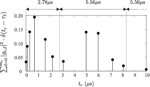
where $i$ denotes the imaginary unit and where the real parameters $|g_{\mathrm{c},\ell}|$, $\theta_{\ell}$, and $\tau_{\ell}$ are the gain, the phase rotation, and the delay introduced by the $\ell$-th path, respectively. Fig. 4 illustrates a typical power-delay profile of a multipath channel that was measured in an urban area with moderate to high tree density [41, Fig. 2.51].

The uplink channel of the NB-IoT occupies a single physical resource block (PRB) from the LTE configuration, and so the bandwidth of the transmitted signal is restricted to $W_{\mathrm{PRB}}=180$ kHz [9, Sec. 5.2.3]. As can be seen from Fig. 4, the delay spread of the wireless channel exceeds the duration of a single channel use ($W_{\mathrm{PRB}}^{-1}=5.56\mu\mathrm{s}$). This issue along with the multipath propagation gives rise to ISI. As shown in Table I, the ISI tap coefficients are captured by sampling at times $\frac{W_{\mathrm{PRB}}^{-1}}{2}+\ell\cdot W_{\mathrm{PRB}}^{-1}$ for $\ell\in\{0,1,2\}$. By ignoring the third tap, due to its relative amplitude being 10dB below the first tap, the sampled output of a filter matched to the shaping pulse at the receiver gives rise to an ISI channel described by $\big{(}g(D)\triangleq 0.792+0.610D,\sigma^{2}\big{)}$.

Before introducing the wiretapping scenario, we consider a point-to-point (P2P) setup where the only channel input constraint is an average-energy constraint. This simplification allows us to use the well-known “water-pouring” formulas for analyzing the capacities of Bob’s and Eve’s P2P channels in the examined ISI-WTC. Let us consider the average-energy constraint per input symbol $E_{\mathrm{s}}$ (in Joules), the symbol duration $T$ (in seconds), a perfect lowpass filter of bandwidth $W\triangleq\frac{1}{2T}$ with the sampling at Nyquist frequency $1/T$ at the receiver, and the power spectral density $N(f)$ (in Watts per Hertz) of the additive Gaussian noise before the lowpass filter. The unconstrained (besides some average-energy constraint) capacity of an ISI channel, described by $\big{(}g(D)=\sum_{t=0}^{m}g_{t}D^{t},N(f)\big{)}$, is given by the “water-pouring” formula (see, e.g.,[42])

$$C(g,W)=\frac{1}{2}\cdot\int\limits_{-\infty}^{\infty}\log^{+}\left(\frac{\alpha}{N(f)/|G(f)|^{2}}\right)\,\mathrm{d}f,$$

where

$$G(f) =\begin{cases}{\displaystyle\frac{\sum_{\ell=0}^{m}g_{\ell}e^{-i2\ell\pi fT}}{\sqrt{\sum_{\ell=0}^{m}|g_{\ell}|^{2}}}}&\text{(if $|f|\leq W$)}\\ 0&\text{(otherwise)}\end{cases},$$

and where $\alpha>0$ is chosen such that

$$E_{\mathrm{s}}=\int\limits_{-\infty}^{\infty}{\left(\alpha-\frac{N(f)}{|G(f)|^{2}}\right)^{\!\!+}}\mathrm{d}f.$$

IV-B Wiretapping Scenarios and Achievable Secure Rates

Figure 5: Results for Example 1, where $g^{\mathrm{B}}(D)=0.792+0.610D$, $g^{\mathrm{E}}(D)=0.446+0.633D+0.633D^{2}$, $\mathrm{SNR}^{\mathrm{E}}_{\textrm{dB}}=-6.0\leavevmode\nobreak\ \text{dB}$. ($a$) Unconstrained capacities of Bob’s and Eve’s P2P channels in $\mathrm{nats}/\mathrm{sec}$ with normalized average-energy constraint $E_{\mathrm{s}}=1\leavevmode\nobreak\ \mathrm{J}$. ($b$) Gain-to-noise power spectrum ratios of Bob’s and Eve’s P2P channels in dB/Hz. ($c$) The power spectrum of a sequence generated by the optimized input Markov source.

Figure 6: Results for Example 2, where $g^{\mathrm{B}}(D)=0.446+0.633D+0.633D^{2}$, $g^{\mathrm{E}}(D)=0.792+0.610D$, $\mathrm{SNR}^{\mathrm{E}}_{\textrm{dB}}=-6.0\leavevmode\nobreak\ \text{dB}$. ($a$) Unconstrained capacities of Bob’s and Eve’s P2P channels in $\mathrm{nats}/\mathrm{sec}$ with normalized average-energy constraint $E_{\mathrm{s}}=1\leavevmode\nobreak\ \mathrm{J}$. ($b$) Gain-to-noise power spectrum ratios of Bob’s and Eve’s P2P channels in dB/Hz. ($c$) The power spectrum of a sequence generated by the optimized input Markov source.

We examine Algorithm 1 for optimizing the parameters of an input Markov source with the alphabet $\mathcal{X}=\{+\sqrt{E_{\mathrm{s}}},-\sqrt{E_{\mathrm{s}}}\}$ and the memory order $\nu=2$ at the input of two different ISI-WTCs. We consider a setup where Bob’s channel and Eve’s channel have normalized transfer polynomials $g^{\mathrm{B}}(D)$ and $g^{\mathrm{E}}(D)$, and additive white Gaussian noises of variances $\sigma_{\mathrm{B}}^{2}$ and $\sigma_{\mathrm{E}}^{2}$, respectively. Accordingly, the signal-to-noise ratios (SNRs) of Bob’s channel and Eve’s channel are defined as, respectively, $\mathrm{SNR}^{\mathrm{B}}\triangleq E_{\mathrm{s}}/\sigma_{\mathrm{B}}^{2}$ and $\mathrm{SNR}^{\mathrm{E}}\triangleq E_{\mathrm{s}}/\sigma_{\mathrm{E}}^{2}$.

Example 1.

In the first scenario, Bob’s channel is assumed to be the ISI channel derived from Table I, i.e.,

$$g^{\mathrm{B}}(D)=0.792+0.610D.$$

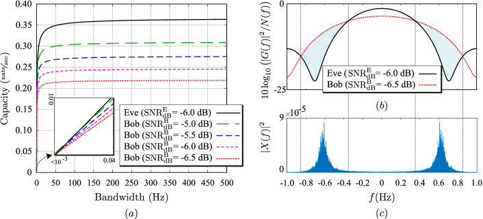
Also, Eve’s channel is assumed to be another ISI channel with the same delay profile as in Table I, but with different tap coefficients. Since it is challenging for Eve to intercept the transmitted signals from the line-of-sight transmission [17], the relative amplitude of Eve’s direct path is assumed to be (at least) $2.5$ dB below Bob’s direct path. However, the other tap coefficients are then assumed to be such that Eve’s channel has the highest unconstrained capacity among all ISI channels satisfying the delay profile of Table I, i.e.,

$$(g^{\mathrm{E}}_{t})_{t=0}^{2}=\arg\max_{\tilde{g}^{\mathrm{E}}:\ |\tilde{g}^{\mathrm{E}}_{0}|\leq|g^{\mathrm{B}}_{0}|-2.5\mathrm{dB}}C(\tilde{g}^{\mathrm{E}},W).$$

Solving this problem for $g^{\mathrm{B}}_{0}=0.792$ leads to

$$g^{\mathrm{E}}(D)=0.446+0.633D+0.633D^{2}.$$

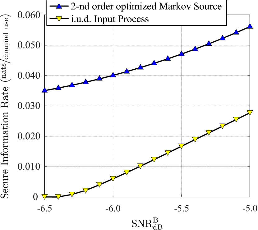
The resulting unconstrained capacities of Bob’s and Eve’s P2P channels are depicted in Fig. 5($a$). It can be seen from Fig. 5($a$) that Eve’s channel has a higher unconstrained capacity than Bob’s channel for sufficiently large enough bandwidth. In this sense, Bob’s channel is “worse” than Eve’s channel. However, luckily for Bob, there are frequencies where Bob’s channel has a better gain-to-noise power spectrum ratio than Eve’s channel, as can be seen from Fig. 5($b$). These spectral discrepancies can be exploited by a suitably tuned input source toward obtaining positive secure rates. Fig. 5($c$) shows the power spectrum of a sequence with the length of $10^{6}$ generated by the optimized Markov source, where the optimization was done with the help of Algorithm 1. It can be seen from Fig. 5($c$) that the optimized Markov source concentrates the available power of the generated input sequence in frequency ranges where Bob’s channel has a higher gain-to-noise power spectrum ratio than Eve’s channel.

Fig. 8 shows the obtained secure rates: on the one hand for an unoptimized Markov source, producing independent and uniformly distributed (i.u.d.) symbols, and, on the other hand, for an optimized Markov source. In this plot, the best obtained secure rate is plotted after running Algorithm 1 for $100$ different initializations. $\square$

In Example 2, we consider the same scenario as in Example 1, but where Bob’s channel is swapped with Eve’s channel. For comparison, note that in a memoryless wiretap channel setup, if the first scenario is such that positive secure rates are possible, then in the second scenario, i.e., after swapping Bob’s channel with Eve’s channel, the secure rate is zero [46].

Figure 7: Example 1: Secure rates achieved by various input processes in nats/channel use.

Figure 8: Example 2: Secure rates achieved by various input processes in nats/channel use.

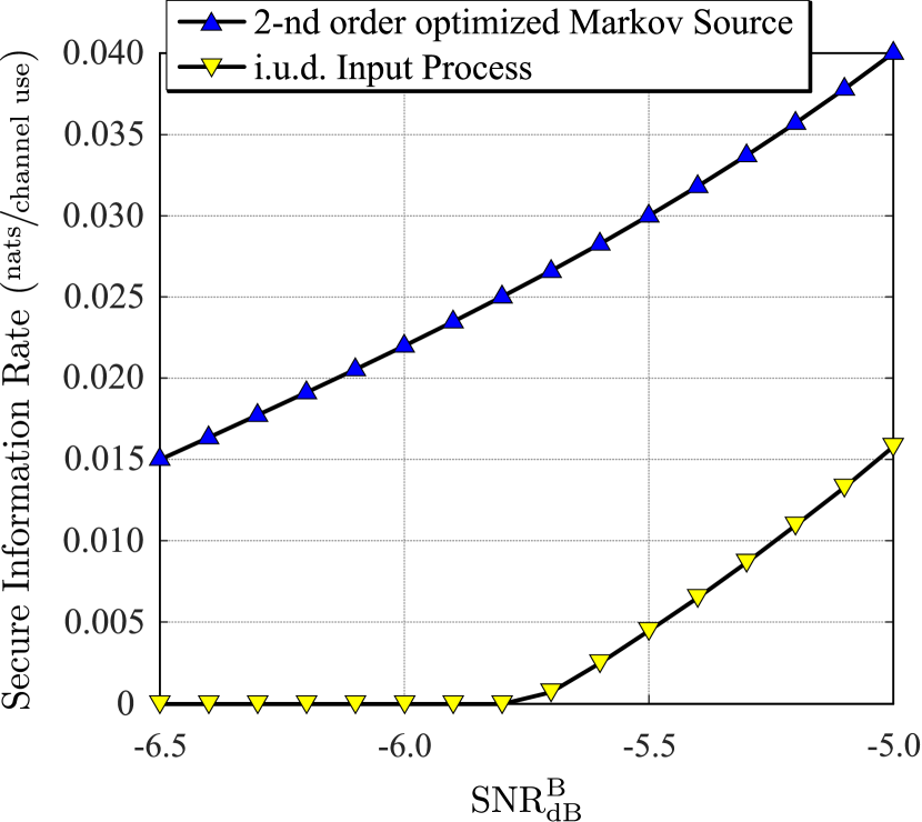
Example 2.

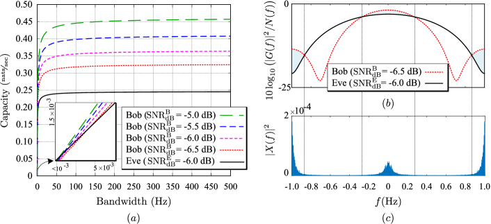
In the second scenario, the roles of the receiver terminals in Example 1 are swapped, i.e.,

$$g^{\mathrm{B}}(D) =0.446+0.633D+0.633D^{2},$$

$$g^{\mathrm{E}}(D) =0.792+0.610D.$$

In this case, Bob’s channel has a higher unconstrained capacity than Eve’s channel for large enough bandwidth (see Fig. 6). In this sense, it is not unexpected that positive secure rates are possible. Nevertheless, it is worthwhile to point out that here positive secure rates are possible even though Bob’s channel has larger memory than Eve’s channel, and for some selections of $\mathrm{SNR}^{\mathrm{B}}_{\textrm{dB}}$, higher noise power than Eve’s channel (see Fig. 8). $\square$

IV-C Discussion

In a memoryless wiretap channel setup, Eve’s channel necessarily has to be noisier than Bob’s channel to achieve a positive secrecy capacity [46]. This results in the capacity of Eve’s channel being less than the capacity of Bob’s channel. Interestingly enough, the optimized Markov sources achieved positive secure rates over the ISI-WTCs, (i) even when the unconstrained capacity of Bob’s channel is smaller than the unconstrained capacity of Eve’s channel (as pointed out in Example 1), (ii) even when Bob’s channel tolerates both a higher noise power and a larger memory compared with Eve’s channel (as pointed out in Example 2). These results confirm the feasibility of optimizing input Markov sources for shaping the available power of the generated sequences toward benefiting from the spectral discrepancies of Bob’s and Eve’s P2P channels—without consuming any extra power for cooperative jamming or injecting artificial noise (as it was done in [31], [32]).

V Conclusion

In this paper, we have derived a lower bound on the achievable secure rates over ISI-WTCs. Then, we have optimized a Markov source at the input of an ISI-WTC toward (locally) maximizing the obtained secure rates. Because directly maximizing the secure rate function is challenging, we have iteratively approximated the secure rate function by concave surrogate functions whose maximum can be found efficiently. Our numerical results show that by implicitly using the discrepancies between the frequency responses of Bob’s channel and Eve’s channel, it is possible to achieve positive secure rates also for setups where the unconstrained capacity of Eve’s channel is larger than the unconstrained capacity of Bob’s channel.

Appendix A Secrecy Criterion

This appendix gives a concise discussion about the employed secrecy criterion. Let $M$ be a random variable corresponding to a uniformly chosen secret message from an alphabet $\mathcal{M}$. (Note that $\mathcal{M}$ implicitly depends on the block length $n$.) Moreover, recall that the sequence observed by Eve is denoted by $\mathbf{Z}_{1}^{n}$ (see Fig. 1). The statistical dependence between $M$ and $\mathbf{Z}_{1}^{n}$ is often measured in terms of the mutual information between $M$ and $\mathbf{Z}_{1}^{n}$ to ensure the information-theoretic perfect secrecy. For instance, the so-called strong secrecy criterion [47] requires $I(M;\mathbf{Z}_{1}^{n})\to 0$ and the so-called weak secrecy criterion [48] requires $\frac{1}{n}I(M;\mathbf{Z}_{1}^{n})\to 0$ as $n\to\infty$. (See also the recent survey [4].)

On one hand, the weak secrecy criterion is easier to achieve, but it might lead to coding schemes that are vulnerable for practical purposes [49, Ch. 3.3]. On the other hand, the strong secrecy criterion is much more desirable, but very difficult to achieve with practical coding schemes [50]. Therefore, in the following, we will use a secrecy criterion that is stronger than the weak secrecy criterion, but more easily achieved than the strong secrecy criterion [50, Proposition 1]. Namely, we use the secrecy criterion (2), based on the variational distance $d_{\mathcal{M}\times\mathcal{Z}^{n}}(p_{M,\mathbf{Z}_{1}^{n}},p_{M}p_{\mathbf{Z}_{1}^{n}})$, which was called $\mathbb{S}_{2}(p_{M,\mathbf{Z}_{1}^{n}},p_{M}p_{\mathbf{Z}_{1}^{n}})$ in [50]. This secrecy measure can be bounded as

$$d_{\mathcal{M}\times\mathcal{Z}^{n}}(p_{M,\mathbf{Z}_{1}^{n}},p_{M}p_{\mathbf{Z}_{1}^{n}})$$

$$=\int_{\mathbf{z}_{1}^{n}\in\mathcal{Z}^{n}}\sum_{m\in\mathcal{M}}p_{M}(m)\cdot\Big{|}p_{\mathbf{Z}_{1}^{n}|M}(\mathbf{z}_{1}^{n}|m)-p_{\mathbf{Z}_{1}^{n}}(\mathbf{z}_{1}^{n})\Big{|}\mathrm{d}\mathbf{z}_{1}^{n}$$

$$=\int_{\mathbf{z}_{1}^{n}\in\mathcal{Z}^{n}}\sum_{m\in\mathcal{M}}p_{M}(m)\cdot\Big{|}p_{\mathbf{Z}_{1}^{n}|M}(\mathbf{z}_{1}^{n}|m)$$

$$\qquad\quad-\sum_{\tilde{m}\in\mathcal{M}}p_{\mathbf{Z}_{1}^{n},M}(\mathbf{z}_{1}^{n},\tilde{m})\Big{|}\ \mathrm{d}\mathbf{z}_{1}^{n}$$

$$\leq\sum_{(m,\tilde{m})\in\mathcal{M}^{2}}p_{M}(m)\cdot p_{M}(\tilde{m})\cdot\int_{\mathbf{z}_{1}^{n}\in\mathcal{Z}^{n}}\Big{|}p_{\mathbf{Z}_{1}^{n}|M}(\mathbf{z}_{1}^{n}|m)$$

$$\qquad\quad-p_{\mathbf{Z}_{1}^{n}|M}(\mathbf{z}_{1}^{n}|\tilde{m})\Big{|}\ \mathrm{d}\mathbf{z}_{1}^{n}$$

$$=\sum_{(m,\tilde{m})\in\mathcal{M}^{2}}p_{M}(m)\cdot p_{M}(\tilde{m})\cdot d_{\mathcal{Z}^{n}}(p_{\mathbf{Z}_{1}^{n}|M=m},p_{\mathbf{Z}_{1}^{n}|M=\tilde{m}}),$$ (15)

where the inequality follows from the triangle inequality. It follows from (15) that satisfying (2) makes $m,\tilde{m}\in\mathcal{M}$ statistically (almost) indistinguishable at Eve’s decoder.

For further context, note that the secrecy criterion in (2) is weaker than the so-called distinguishing secrecy criterion in cryptography [51], which requires

$$\max\limits_{(m,\tilde{m})\in\mathcal{M}^{2}}\!\big{(}d_{\mathcal{Z}^{n}}(p_{\mathbf{Z}_{1}^{n}|M=m},p_{\mathbf{Z}_{1}^{n}|M=\tilde{m}})\big{)}\to 0,$$

as $n\to\infty$, and which is equivalent to the so-called semantic secrecy criterion. As a consequence, satisfying (2) gives rise to a loosened notion of the semantic security. This looseness arises from the extra assumption that $p_{M}$ is fixed and known, contrary to the cryptographically relevant secrecy criteria.

Appendix B Proof of Proposition 1

We start by defining the notations that will be used in this appendix. The mutual information density between the respective realizations of random variables $X$ and $Y$ is defined to be

$$i(x;y)\triangleq\log\left(\frac{p_{X,Y}(x,y)}{p_{X}(x)\cdot p_{Y}(y)}\right).$$

Moreover, the conditional mutual information density between the respective realizations of random variables $X$ and $Y$ given $Z=z$ is defined to be

$$i(x;y|z)\triangleq\log\left(\frac{p_{X,Y|Z}(x,y|z)}{p_{X|Z}(x|z)\cdot p_{Y|Z}(y|z)}\right).$$

Consequently, we have

$$I(X;Y) =\sum_{x,y}p_{X,Y}(x,y)\cdot i(x;y),$$

$$I(X;Y|Z) =\sum_{x,y,z}p_{X,Y,Z}(x,y,z)\cdot i(x;y|z).$$

Following [53], the spectral sup/inf-mutual information rates are defined to be

$$\operatorname{p-}\!\limsup_{n\to\infty} \frac{1}{n}{i}(\mathbf{X}_{1}^{n};\mathbf{Y}_{1}^{n})$$

$$\triangleq\inf\left\{\alpha:\lim_{n\to\infty}\operatorname{Pr}\left(\frac{1}{n}{i}(\mathbf{X}_{1}^{n};\mathbf{Y}_{1}^{n})>\alpha\right)=0\right\},$$

$$\operatorname{p-}\!\liminf_{n\to\infty} \frac{1}{n}{i}(\mathbf{X}_{1}^{n};\mathbf{Y}_{1}^{n})$$

$$\triangleq\sup\left\{\beta:\lim_{n\to\infty}\operatorname{Pr}\left(\frac{1}{n}{i}(\mathbf{X}_{1}^{n};\mathbf{Y}_{1}^{n})<\beta\right)=0\right\}.$$

According to [54, Lemma 2], for an arbitrary wiretap channel $\bigl{(}\mathcal{X}$, $\{p_{\mathbf{Y}_{1}^{n},\mathbf{Z}_{1}^{n}|\mathbf{X}_{1}^{n}}(\mathbf{y}_{1}^{n},\mathbf{z}_{1}^{n}|\mathbf{x}_{1}^{n})\}_{n=1}^{\infty}$, $\mathcal{Y}$, $\mathcal{Z}\bigr{)}$ consisting of an arbitrary input alphabet $\mathcal{X}$, two arbitrary output alphabets $\mathcal{Y}$ and $\mathcal{Z}$ corresponding to Bob’s and Eve’s observations, respectively, and a sequence of transition probabilities $\{p_{\mathbf{Y}_{1}^{n},\mathbf{Z}_{1}^{n}|\mathbf{X}_{1}^{n}}(\mathbf{y}_{1}^{n},\mathbf{z}_{1}^{n}|\mathbf{x}_{1}^{n})\}_{n=1}^{\infty}$, all secure rates $R_{\mathrm{s}}$ satisfying

$$R_{\mathrm{s}} \!\!<\!\!\!\max_{\{\mathbf{X}_{1}^{n}\}_{n=1}^{\infty}}\!\!\!\left(\!\operatorname{p-}\!\liminf_{n\to\infty}\!\frac{1}{n}{i}(\mathbf{X}_{1}^{n};\mathbf{Y}_{1}^{n})-\operatorname{p-}\!\limsup_{n\to\infty}\!\frac{1}{n}{i}(\mathbf{X}_{1}^{n};\mathbf{Z}_{1}^{n})\!\right)^{\!\!\!+}$$

are achievable under the reliability criterion (1) and the secrecy criterion (2). We leverage [54, Lemma 2] for deducing a lower bound on the achievable secure rates over ISI-WTCs.

Consider an ISI-WTC as in Definition 1. For all positive integers $\ell$ and $\nu\geq\max(m_{\mathrm{B}},m_{\mathrm{E}})$, let $\bigl{\{}\mathbf{X}_{k(\ell+2\nu)-\nu+1}^{k(\ell+2\nu)+(\ell+\nu)}\bigr{\}}_{k=-\infty}^{+\infty}$ be a block i.i.d. process where each block has length $\ell+2\nu$. So, it suffices to specify the distribution of a single block $\mathbf{X}_{k(\ell+2\nu)-\nu+1}^{k(\ell+2\nu)+(\ell+\nu)}$. In order to ensure that there is no interference across blocks, we set

$$X_{k(\ell+2\nu)+(\ell+1)} \triangleq 0,\quad\ldots,\quad X_{k(\ell+2\nu)+(\ell+\nu)}\triangleq 0,$$

while allowing $\mathbf{X}_{k(\ell+2\nu)-\nu+1}^{k(\ell+2\nu)+\ell}$ to be arbitrarily distributed. Obviously,

$$\bigl{\{}\mathbf{X}_{k(\ell+2\nu)-\nu+1}^{k(\ell+2\nu)+(\ell+\nu)},\mathbf{Y}_{k(\ell+2\nu)-\nu+1}^{k(\ell+2\nu)+(\ell+\nu)}\bigr{\}}_{k=-\infty}^{+\infty}$$

is a joint block i.i.d. process. Similarly,

$$\bigl{\{}\mathbf{X}_{k(\ell+2\nu)-\nu+1}^{k(\ell+2\nu)+(\ell+\nu)},\mathbf{Z}_{k(\ell+2\nu)-\nu+1}^{k(\ell+2\nu)+(\ell+\nu)}\bigr{\}}_{k=-\infty}^{+\infty}$$

is also a joint block i.i.d. process. Let

$$\{X_{t},Y_{t}\}_{t=1}^{n}=\bigl{\{}\mathbf{X}_{k(\ell+2\nu)-\nu+1}^{k(\ell+2\nu)+(\ell+\nu)},\mathbf{Y}_{k(\ell+2\nu)-\nu+1}^{k(\ell+2\nu)+(\ell+\nu)}\bigr{\}}_{k=1}^{n^{\prime}\!},$$

where $n^{\prime}$ denotes the number of i.i.d. blocks in $\{X_{t}\}_{t=1}^{n}$. Then,

$$\lim_{n\to\infty}\frac{1}{n}i(\mathbf{X}_{1}^{n};\mathbf{Y}_{1}^{n})$$

$$=n^{\prime}\cdot\lim_{n\to\infty}\frac{1}{n}\left(\!\frac{1}{n^{\prime}}\sum_{k=1}^{n^{\prime}\!}i\big{(}\mathbf{X}_{k(\ell+2\nu)-\nu+1}^{k(\ell+2\nu)+(\ell+\nu)};\mathbf{Y}_{k(\ell+2\nu)-\nu+1}^{k(\ell+2\nu)+(\ell+\nu)}\big{)}\!\!\right)$$

$$=\frac{1}{\ell+2\nu}I(\mathbf{X}_{-\nu+1}^{\ell+\nu};\mathbf{Y}_{-\nu+1}^{\ell+\nu}),\qquad\text{w.p.\ $1$,}$$ (16)

where the second equality follows from the strong law of large numbers and $n=n^{\prime}\cdot(\ell+2\nu)$. With an analogous manipulation, we have

$$\lim_{n\to\infty}\frac{1}{n}i(\mathbf{X}_{1}^{n};\mathbf{Z}_{1}^{n})=\frac{1}{\ell+2\nu}I(\mathbf{X}_{-\nu+1}^{\ell+\nu};\mathbf{Z}_{-\nu+1}^{\ell+\nu}),\qquad\text{w.p.\leavevmode\nobreak\ $1$}.$$ (17)

Note

$$I(\mathbf{X}_{-\nu+1}^{\ell+\nu};\mathbf{Y}_{-\nu+1}^{\ell+\nu}) \geq I(\mathbf{X}_{-\nu+1}^{\ell};\mathbf{Y}_{1}^{\ell})$$

$$=I(\mathbf{X}_{-\nu+1}^{0};\mathbf{Y}_{1}^{\ell})+I(\mathbf{X}_{1}^{\ell};\mathbf{Y}_{1}^{\ell}|\mathbf{X}_{-\nu+1}^{0})$$

$$\geq I(\mathbf{X}_{1}^{\ell};\mathbf{Y}_{1}^{\ell}|\mathbf{X}_{-\nu+1}^{0}).$$

Moreover,

$$I(\mathbf{X}_{-\nu+1}^{\ell+\nu};\mathbf{Z}_{-\nu+1}^{\ell+\nu})$$

$$=I(\mathbf{X}_{-\nu+1}^{\ell};\mathbf{Z}_{-\nu+1}^{\ell+\nu})$$

$$=I(\mathbf{X}_{-\nu+1}^{\ell};\mathbf{Z}_{1}^{\ell})+I(\mathbf{X}_{-\nu+1}^{\ell};\mathbf{Z}_{-\nu+1}^{0}|\mathbf{Z}_{1}^{\ell})$$

$$\quad\ +I(\mathbf{X}_{-\nu+1}^{\ell};\mathbf{Z}_{\ell+1}^{\ell+\nu}|\mathbf{Z}_{-\nu+1}^{\ell})$$

$$=I(\mathbf{X}_{1}^{\ell};\mathbf{Z}_{1}^{\ell}|\mathbf{X}_{-\nu+1}^{0})+I(\mathbf{X}_{-\nu+1}^{0};\mathbf{Z}_{1}^{\ell})$$

$$\quad\ +I(\mathbf{X}_{-\nu+1}^{\ell};\mathbf{Z}_{-\nu+1}^{0}|\mathbf{Z}_{1}^{\ell})+I(\mathbf{X}_{-\nu+1}^{\ell};\mathbf{Z}_{\ell+1}^{\ell+\nu}|\mathbf{Z}_{-\nu+1}^{\ell})$$

$$=I(\mathbf{X}_{1}^{\ell};\mathbf{Z}_{1}^{\ell}|\mathbf{X}_{-\nu+1}^{0})+I(\mathbf{X}_{-\nu+1}^{0};\mathbf{Z}_{1}^{\ell})$$

$$\quad\ +I(\mathbf{X}_{-\nu+1}^{0};\mathbf{Z}_{-\nu+1}^{0}|\mathbf{Z}_{1}^{\ell})+I(\mathbf{X}_{\ell-\nu+1}^{\ell};\mathbf{Z}_{\ell+1}^{\ell+\nu}|\mathbf{Z}_{-\nu+1}^{\ell})$$

$$\leq I(\mathbf{X}_{1}^{\ell};\mathbf{Z}_{1}^{\ell}|\mathbf{X}_{-\nu+1}^{0})+3\nu\log|\mathcal{X}|.$$

Combining [54, Lemma 2] with (16), (17), and the above lower and upper bounds implies that all secure rates $R_{\mathrm{s}}$ satisfying

$$R_{\mathrm{s}} <\frac{1}{\ell+2\nu}\Big{(}I(\mathbf{X}_{1}^{\ell};\mathbf{Y}_{1}^{\ell}|\mathbf{X}_{-\nu+1}^{0})-I(\mathbf{X}_{1}^{\ell};\mathbf{Z}_{1}^{\ell}|\mathbf{X}_{-\nu+1}^{0})$$

$$\hskip 56.9055pt-3\nu\cdot\log|\mathcal{X}|\Big{)}^{+}$$ (18)

are achievable under the reliability criterion (1) and the secrecy criterion (2).

Let $\nu$ be the memory order of an FSMC associated with the considered ISI-WTC and let $\mathbf{Q}\in\mathcal{Q}(\mathcal{B})$ be the parameter of the input Markov source. Define

$$R_{\mathrm{s}}(\mathbf{Q})\triangleq\lim_{n\to\infty}\frac{1}{n}\Big{(}I(\mathbf{S}_{1}^{n};\mathbf{Y}_{1}^{n}|S_{0})-I(\mathbf{S}_{1}^{n};\mathbf{Z}_{1}^{n}|S_{0})\Big{)}^{+}.$$

It is easy to verify

$$I(\mathbf{X}_{1}^{n};\mathbf{Y}_{1}^{n}|\mathbf{X}_{-\nu+1}^{0}) =I(\mathbf{S}_{1}^{n};\mathbf{Y}_{1}^{n}|S_{0}),$$

$$I(\mathbf{X}_{1}^{n};\mathbf{Z}_{1}^{n}|\mathbf{X}_{-\nu+1}^{0}) =I(\mathbf{S}_{1}^{n};\mathbf{Z}_{1}^{n}|S_{0}).$$

By letting $n\to\infty$ and invoking (18), all secure rates $R_{\mathrm{s}}$ satisfying $R_{\mathrm{s}}<R_{\mathrm{s}}(\mathbf{Q})$ are achievable. Finally, reformulating the expression of $R_{\mathrm{s}}(\mathbf{Q})$ as follows proves the promised result.

$$R_{\mathrm{s}}(\mathbf{Q}) =\lim_{n\to\infty}\frac{1}{n}\sum_{t=1}^{n}\bigl{(}I(S_{t};\mathbf{Y}_{1}^{n}|\mathbf{S}_{0}^{t-1})-I(S_{t};\mathbf{Z}_{1}^{n}|\mathbf{S}_{0}^{t-1})\bigr{)}$$

$$=\lim_{n\to\infty}\frac{1}{n}\sum_{t=1}^{n}\bigl{(}I(S_{t};\mathbf{Y}_{1}^{n}|S_{t-1})-I(S_{t};\mathbf{Z}_{1}^{n}|S_{t-1})\bigr{)}$$

$$=\lim_{n\to\infty}\frac{1}{n}\sum_{t=1}^{n}\bigl{(}H(S_{t}|\mathbf{Z}_{1}^{n},S_{t-1})-H(S_{t}|\mathbf{Y}_{1}^{n},S_{t-1})\bigr{)}$$

$$=\sum_{(i,j)\in\mathcal{B}}Q_{ij}\cdot\bigl{(}T^{\mathrm{B}}_{ij}(\mathbf{Q})-T^{\mathrm{E}}_{ij}(\mathbf{Q})\bigr{)},$$

where the $(\cdot)^{+}$ operator has been omitted for clarity of the presentation and where the last equality is based on expressing $H(S_{t}|\mathbf{Y}_{1}^{n},S_{t-1})$ as (19) at the top of this page,

$$H(S_{t}|\mathbf{Y}_{1}^{n},S_{t-1}) =-\sum_{(i,j)\in\mathcal{B}}{\int_{\mathbf{y}_{1}^{n}\in\mathcal{Y}^{n}}}p_{S_{t},S_{t-1},\mathbf{Y}_{1}^{n}}(j,i,\mathbf{y}_{1}^{n})\cdot\log\bigl{(}p_{S_{t}|S_{t-1},\mathbf{Y}_{1}^{n}}(j|i,\mathbf{y}_{1}^{n})\bigr{)}{\mathrm{d}\mathbf{y}_{1}^{n}}$$

$$=-\sum_{(i,j)\in\mathcal{B}}{\int_{\mathbf{y}_{1}^{n}\in\mathcal{Y}^{n}}}p_{S_{t},S_{t-1},\mathbf{Y}_{1}^{n}}(j,i,\mathbf{y}_{1}^{n})\cdot\left(\log\left(\frac{p_{S_{t},S_{t-1},\mathbf{Y}_{1}^{n}}(j,i,\mathbf{y}_{1}^{n})}{p_{\mathbf{Y}_{1}^{n}}(\mathbf{y}_{1}^{n})}\right)-\log\left(\frac{p_{S_{t-1},\mathbf{Y}_{1}^{n}}(i,\mathbf{y}_{1}^{n})}{p_{\mathbf{Y}_{1}^{n}}(\mathbf{y}_{1}^{n})}\right)\right){\mathrm{d}\mathbf{y}_{1}^{n}}$$

$$=-\sum_{(i,j)\in\mathcal{B}}\mu_{i}p_{ij}\cdot{\int_{\mathbf{y}_{1}^{n}\in\mathcal{Y}^{n}}}\Bigl{(}p_{\mathbf{Y}_{1}^{n}|S_{t-1},S_{t}}(\mathbf{y}_{1}^{n}|i,j)\cdot\log\bigl{(}p_{S_{t-1},S_{t}|\mathbf{Y}_{1}^{n}}(i,j|\mathbf{y}_{1}^{n})\bigr{)}$$

$$\hskip 170.71652pt-p_{\mathbf{Y}_{1}^{n}|S_{t-1}}(\mathbf{y}_{1}^{n}|i)\cdot\log\bigl{(}p_{S_{t-1}|\mathbf{Y}_{1}^{n}}(i|\mathbf{y}_{1}^{n})\bigr{)}\Bigr{)}{\mathrm{d}\mathbf{y}_{1}^{n}}$$

$$=-\sum_{(i,j)\in\mathcal{B}}\mu_{i}p_{ij}\cdot{\int_{\mathbf{y}_{1}^{n}\in\mathcal{Y}^{n}}}\Biggl{(}\frac{p_{S_{t-1},S_{t}|\mathbf{Y}_{1}^{n}}(i,j|\mathbf{y}_{1}^{n})}{\mu_{i}p_{ij}}\cdot p_{\mathbf{Y}_{1}^{n}}(\mathbf{y}_{1}^{n})\cdot\log\bigl{(}p_{S_{t-1},S_{t}|\mathbf{Y}_{1}^{n}}(i,j|\mathbf{y}_{1}^{n})\bigr{)}$$

$$\hskip 170.71652pt-\frac{p_{S_{t-1}|\mathbf{Y}_{1}^{n}}(i|\mathbf{y}_{1}^{n})}{\mu_{i}}\cdot p_{\mathbf{Y}_{1}^{n}}(\mathbf{y}_{1}^{n})\cdot\log\bigl{(}p_{S_{t-1}|\mathbf{Y}_{1}^{n}}(i|\mathbf{y}_{1}^{n})\bigr{)}\Biggr{)}{\mathrm{d}\mathbf{y}_{1}^{n}}$$

$$=-\sum_{(i,j)\in\mathcal{B}}\mu_{i}p_{ij}\cdot\left({\int_{\mathbf{y}_{1}^{n}\in\mathcal{Y}^{n}}}p_{\mathbf{Y}_{1}^{n}}(\mathbf{y}_{1}^{n})\cdot\log\left(\frac{p_{S_{t-1},S_{t}|\mathbf{Y}_{1}^{n}}(i,j|\mathbf{y}_{1}^{n})^{{p_{S_{t-1},S_{t}|\mathbf{Y}_{1}^{n}}(i,j|\mathbf{y}_{1}^{n})}/\mu_{i}p_{ij}}}{p_{S_{t-1}|\mathbf{Y}_{1}^{n}}(i|\mathbf{y}_{1}^{n})^{{p_{S_{t-1}|\mathbf{Y}_{1}^{n}}(i|\mathbf{y}_{1}^{n})}/\mu_{i}}}\right)\right){\mathrm{d}\mathbf{y}_{1}^{n}}.$$ (19)

with an analogous expression for $H(S_{t}|\mathbf{Z}_{1}^{n},S_{t-1})$, along with using (3) and (4).

Appendix C Proof of Lemma 3

Besides the assumptions on the parameterizations $\mathbf{Q}(\theta)$ made in Remark 1, we will also assume that for all $(i,j)\in\mathcal{B}$, the functions $Q_{ij}(\theta)$ and $\mu_{i}(\theta)$ are affine functions in terms of $\theta$, which implies $Q_{ij}^{\theta\theta}(\theta)=0$ and $\mu_{i}^{\theta\theta}(\theta)=0$, where the superscript $\theta\theta$ denotes the second-order derivative w.r.t. $\theta$.

Denoting the second-order derivative of $\bar{\psi}_{\tilde{\mathbf{Q}}}(\theta)$ by $\bar{\psi}_{\tilde{\mathbf{Q}}}^{\theta\theta}(\theta)$, we observe that the claim in the lemma statement is equivalent to $\bar{\psi}_{\tilde{\mathbf{Q}}}^{\theta\theta}(\theta)\geq 0$ for all possible parameterizations of $\mathbf{Q}(\theta)$ that satisfy the above-mentioned conditions.

Let $\hat{Q}_{ij}\triangleq(1-\kappa)\cdot\tilde{Q}_{ij}+\kappa\cdot Q_{ij}$ and $\hat{\mu}_{i}\triangleq(1-\kappa)\cdot\tilde{\mu}_{i}+\kappa\cdot Q_{ij}$ for all $(i,j)\in\mathcal{B}$. Some straightforward calculations show that

$$\bar{\psi}_{\tilde{\mathbf{Q}}}^{\theta\theta}(\theta) =\kappa^{2}\kappa^{\prime}\cdot\left(\sum_{(i,j)\in\mathcal{B}}\frac{(Q^{\theta}_{ij})^{2}}{\hat{Q}_{ij}}-\sum_{i\in\mathcal{S}}\frac{(\mu_{i}^{\theta})^{2}}{\hat{\mu}_{i}}\right)$$

$$=\kappa^{2}\kappa^{\prime}\cdot\sum_{i\in\mathcal{S}}\left(\left(\sum_{j\in\overrightarrow{\mathcal{S}}_{\!i}}\frac{(Q^{\theta}_{ij})^{2}}{\hat{Q}_{ij}}\right)-\frac{(\mu_{i}^{\theta})^{2}}{\hat{\mu}_{i}}\right).$$

Noting that for any $i\in\mathcal{S}$ it holds that

$$\sum_{j\in\overrightarrow{\mathcal{S}}_{\!i}}\frac{(Q^{\theta}_{ij})^{2}}{\hat{Q}_{ij}} =\hat{\mu}_{i}\cdot\sum_{j\in\overrightarrow{\mathcal{S}}_{\!i}}\frac{\hat{Q}_{ij}}{\hat{\mu}_{i}}\cdot\left(\frac{Q^{\theta}_{ij}}{\hat{Q}_{ij}}\right)^{2}$$

$$\geq\hat{\mu}_{i}\cdot\left(\sum_{j\in\overrightarrow{\mathcal{S}}_{\!i}}\frac{\hat{Q}_{ij}}{\hat{\mu}_{i}}\cdot\frac{Q^{\theta}_{ij}}{\hat{Q}_{ij}}\right)^{2}$$

$$=\frac{1}{\hat{\mu}_{i}}\cdot\left(\sum_{j\in\overrightarrow{\mathcal{S}}_{\!i}}Q^{\theta}_{ij}\right)^{2}=\frac{(\mu_{i}^{\theta})^{2}}{\hat{\mu}_{i}},$$

where the inequality follows from Jensen’s inequality, we can conclude that, indeed, $\bar{\psi}_{\tilde{\mathbf{Q}}}^{\theta\theta}(\theta)\geq 0$.

Appendix D Proof of Proposition 2

Maximizing $\psi_{\tilde{\mathbf{Q}}}(\mathbf{Q})$ over $\mathbf{Q}\in\mathcal{Q}(\mathcal{B})$ means to optimize a differentiable, concave function over a polytope. We therefore set up the Lagrangian

$$L \triangleq\sum_{(i,j)\in\mathcal{B}}Q_{ij}\cdot\bigl{(}\tilde{T}^{\mathrm{B}}_{ij}-\tilde{T}^{\mathrm{E}}_{ij}\bigr{)}-\bar{\psi}_{\tilde{\mathbf{Q}}}(\mathbf{Q})$$

$$+\lambda\cdot\left(\sum_{(i,j)\in\mathcal{B}}\!\!\!Q_{ij}-1\right)+\sum_{(i,j)\in\mathcal{B}}\!\!\!\lambda_{j}Q_{ij}-\sum_{(i,j)\in\mathcal{B}}\!\!\!\lambda_{i}Q_{ij}.$$

Note that at this stage we omit Lagrangian multipliers w.r.t. the constraints $Q_{ij}\geq 0$, $(i,j)\in\mathcal{B}$. We will make sure at a later stage that these constraints are satisfied thanks to the choice of $\kappa$ in (13).

Recall that we assume that the surrogate function takes on its maximal value at $\mathbf{Q}=\mathbf{Q}^{*}$. Therefore, setting the gradient of $L$ equal to the zero vector at $\mathbf{Q}=\mathbf{Q}^{*}$, we obtain

$$0 =\left.\frac{\partial L}{\partial Q_{ij}}\right|_{\mathbf{Q}=\mathbf{Q}^{*}} =\tilde{T}^{\mathrm{B}}_{ij}-\tilde{T}^{\mathrm{E}}_{ij}-\left.\frac{\partial\bar{\psi}_{\tilde{\mathbf{Q}}}(\mathbf{Q})}{\partial Q_{ij}}\right|_{\mathbf{Q}=\mathbf{Q}^{*}}+\lambda^{*}+\lambda_{j}^{*}-\lambda_{i}^{*},$$

$$\hskip 156.49014pt(i,j)\in\mathcal{B},$$ (20)

$$0 =\left.\frac{\partial L}{\partial\lambda}\right|_{\mathbf{Q}=\mathbf{Q}^{*}} =\sum_{(i,j)\in\mathcal{B}}Q^{*}_{ij}-1,$$

$$0 =\left.\frac{\partial L}{\partial\lambda_{i}}\right|_{\mathbf{Q}=\mathbf{Q}^{*}} =\sum_{r\in\overleftarrow{\mathcal{S}}_{\!i}}Q_{ri}^{*}-\sum_{j\in\overrightarrow{\mathcal{S}}_{\!i}}Q^{*}_{ij},\hskip 71.13188pti\in\mathcal{S},$$

where

$$\left.\frac{\partial\bar{\psi}_{\tilde{\mathbf{Q}}}(\mathbf{Q})}{\partial Q_{ij}}\right|_{\mathbf{Q}=\mathbf{Q}^{*}}$$

$$\,=\left.\kappa^{\prime}\cdot\Bigl{(}\kappa{\cdot}\log\bigl{(}1+\kappa{\cdot}(\delta Q)_{ij}\bigr{)}-\kappa{\cdot}\log\bigl{(}1+\kappa{\cdot}(\delta\mu)_{i}\bigr{)}\Bigr{)}\right|_{\mathbf{Q}=\mathbf{Q}^{*}}$$

$$\,=\kappa\cdot\kappa^{\prime}\cdot\log\left(\frac{(1-\kappa)\cdot\tilde{Q}_{ij}+\kappa\cdot Q^{*}_{ij}}{(1-\kappa)\cdot\tilde{\mu}_{i}+\kappa\cdot\mu^{*}_{i}}\cdot\frac{\tilde{\mu}_{i}}{\tilde{Q}_{ij}}\right)$$

$$\,=\kappa\cdot\kappa^{\prime}\cdot\log\left(\frac{\hat{Q}^{*}_{ij}}{\hat{\mu}_{i}^{*}}\cdot\frac{\tilde{\mu}_{i}}{\tilde{Q}_{ij}}\right)$$

$$\,=\kappa\cdot\kappa^{\prime}\cdot\log(\hat{p}^{*}_{ij})-\kappa\cdot\kappa^{\prime}\cdot\log(\tilde{p}_{ij}).$$ (21)

Here the third and the fourth equality use $\{\hat{Q}^{*}_{ij}\}_{(i,j)\in\mathcal{B}}$, which is defined by

$$\hat{Q}^{*}_{ij} \triangleq(1-\kappa)\cdot\tilde{Q}_{ij}+\kappa\cdot Q^{*}_{ij},\quad(i,j)\in\mathcal{B},$$ (22)

along with $\{\hat{\mu}^{*}_{i}\}_{i\in\mathcal{S}}$ and $\{\hat{p}_{ij}^{*}\}_{(i,j)\in\mathcal{B}}$, which are derived from $\{\hat{Q}^{*}_{ij}\}_{(i,j)\in\mathcal{B}}$ in the usual manner. Note that $\hat{\mu}^{*}_{i}\triangleq\sum_{j^{\prime}\in\overrightarrow{\mathcal{S}}_{\!i}}\hat{Q}^{*}_{ij^{\prime}}=(1-\kappa)\cdot\tilde{\mu}_{i}+\kappa\cdot\mu_{i}^{*}$, for all $i\in\mathcal{S}$, and

$$\hat{p}^{*}_{ij} =\frac{\hat{Q}^{*}_{ij}}{\hat{\mu}^{*}_{i}}=\frac{(1-\kappa)\cdot\tilde{Q}_{ij}+\kappa\cdot Q^{*}_{ij}}{(1-\kappa)\cdot\tilde{\mu}_{i}+\kappa\cdot\mu_{i}^{*}}$$

$$=\frac{(1-\kappa)\cdot\tilde{Q}_{ij}+\kappa\cdot Q^{*}_{ij}}{(1-\kappa)\cdot\tilde{\mu}_{i}+\kappa\cdot\sum_{j^{\prime}\in\overrightarrow{\mathcal{S}}_{\!i}}Q_{ij^{\prime}}^{*}},\quad(i,j)\in\mathcal{B}.$$ (23)

Note also that solving (22) for $Q^{*}_{ij}$ results in

$$Q^{*}_{ij}=\frac{1}{\kappa}\cdot(\hat{Q}^{*}_{ij}-\tilde{Q}_{ij}+\kappa\cdot\tilde{Q}_{ij}),\quad(i,j)\in\mathcal{B},$$

which shows that $Q^{*}_{ij}\geq 0$, $(i,j)\in\mathcal{B}$, for $\kappa$ satisfying (13). (Recall that when setting up the Lagrangian, we omitted the Lagrange multipliers for the constraints $Q_{ij}\geq 0$, $(i,j)\in\mathcal{B}$; therefore we have to verify that the solution satisfies these constraints, which it does indeed.)

Combining (20) and (21), and solving for $\hat{p}^{*}_{ij}$ results in

$$\hat{p}^{*}_{ij}=\tilde{p}_{ij}\cdot\exp\left(\frac{\tilde{T}^{\mathrm{B}}_{ij}-\tilde{T}^{\mathrm{E}}_{ij}+\lambda^{*}+\lambda_{j}^{*}-\lambda_{i}^{*}}{\kappa\kappa^{\prime}}\right),\quad(i,j)\in\mathcal{B}.$$

Using (11) and defining $\rho\triangleq\exp\bigl{(}-\frac{\lambda^{*}}{\kappa\kappa^{\prime}}\bigr{)}$ and $\bm{\gamma}=\bigl{(}\gamma_{i}\triangleq\exp\bigl{(}\frac{\lambda_{i}^{*}}{\kappa\kappa^{\prime}}\bigr{)}\bigr{)}_{i\in\mathcal{S}}$, we rewrite this equation as

$$\hat{p}^{*}_{ij}=\frac{A_{ij}}{\rho}\cdot\frac{\gamma_{j}}{\gamma_{i}},\quad(i,j)\in\mathcal{B}.$$

Because $\sum_{j\in\overrightarrow{\mathcal{S}}_{\!i}}\hat{p}^{*}_{ij}=1$ for all $i\in\mathcal{S}$, summing both sides of this equation over $j\in\overrightarrow{\mathcal{S}}_{\!i}$ results in

$$1=\sum_{j\in\overrightarrow{\mathcal{S}}_{\!i}}\frac{A_{ij}}{\rho}\cdot\frac{\gamma_{j}}{\gamma_{i}},\quad i\in\mathcal{S},$$

or, equivalently,

$$\rho\cdot\gamma_{i}=\sum_{j\in\overrightarrow{\mathcal{S}}_{\!i}}A_{ij}\cdot\gamma_{j},\quad i\in\mathcal{S}.$$

This system of linear equations can be written as

$$\mathbf{A}\cdot\bm{\gamma}=\rho\cdot\bm{\gamma}.$$

Clearly, this equation can only be satisfied if $\bm{\gamma}$ is an eigenvector of $\mathbf{A}$ with corresponding eigenvalue $\rho$. A slightly lengthy calculation (which is somewhat similar to the calculation in [22, Eq. (51)]) shows that

$$\psi_{\tilde{\mathbf{Q}}}(\mathbf{Q}^{*})=\log(\rho).$$ (24)

Clearly, in order to maximize the right-hand side of (24) over all eigenvalues of $\mathbf{A}$, the eigenvalue $\rho$ has to be the Perron–Frobenius eigenvalue and $\bm{\gamma}$ the corresponding eigenvector.

The proof is concluded by noting that (23) can be rewritten as the system of linear equations

$$Q^{*}_{ij}-\hat{p}_{ij}^{*}\cdot\sum_{j^{\prime}\in\overrightarrow{\mathcal{S}}_{\!i}}Q_{ij^{\prime}}^{*}=\frac{1-\kappa}{\kappa}\cdot\bigl{(}\tilde{\mu}_{i}\hat{p}^{*}_{ij}-\tilde{Q}_{ij}\bigr{)},\quad(i,j)\in\mathcal{B},$$

which can be used to determine $\{Q^{*}_{ij}\}_{(i,j)\in\mathcal{B}}$, because all other quantities appearing in these equations are either known or have already been calculated.

Aria Nouri (Graduate Student Member, IEEE) received his M.Sc. degree in electrical engineering, communications, from Shahid-Beheshti University, Tehran, Iran, in 2021. He has been with the cognitive telecommunication research group at Shahid-Beheshti University as a research assistant since 2017. His research interests lie in the areas of coding and information theory, focusing on secure communication, semantic communication, quantum error correction,  and  fault-tolerant  quantum  computing.

Reza Asvadi (Senior Member, IEEE) received the B.Sc. degree (with highest honors) in electrical engineering from K. N. Toosi University of Technology, Tehran, Iran, in 2001, the M.Sc. degree in electrical engineering from Sharif University of Technology, Tehran, Iran, in 2003, and the Ph.D. degree from K. N. Toosi University of Technology, in 2011. From 2004 to 2006, he was a Lecturer with Army Airforce University, Tehran, to fulfill his national service. He was a Post-Doctoral Researcher with the University of Oulu, Oulu, Finland, from 2012 to 2014. During the postdoc, he participated in many Academy of Finland and European Union (FP7) projects investigating iterative algorithms and information-theoretical bounds over new emerging wireless networks. He is currently an Assistant Professor with Shahid Beheshti University, Tehran, since 2016. His research interests include coding and information theory and signal processing for wireless communications. Dr. Asvadi was a recipient of several post-doctoral research grants, including the University of Alberta (2011–2012) and Carleton University (2014–2016) Postdoctoral Fellowships.

Jun Chen (Senior Member, IEEE) received the B.E. degree in communication engineering from Shanghai Jiao Tong University, Shanghai, China, in 2001, and the M.S. and Ph.D. degrees in electrical and computer engineering from Cornell University, Ithaca, NY, USA, in 2004 and 2006, respectively. From September 2005 to July 2006, he was a Post-Doctoral Research Associate with the Coordinated Science Laboratory, University of Illinois at Urbana–Champaign, Urbana, IL, USA, and a Post-Doctoral Fellow with the IBM Thomas J. Watson Research Center, Yorktown Heights, NY, USA, from July 2006 to August 2007. Since September 2007, he has been with the Department of Electrical and Computer Engineering, McMaster University, Hamilton, ON, Canada, where he is currently a Professor. His research interests include information theory, machine learning, wireless communications, and signal processing. Dr. Chen was a recipient of the Josef Raviv Memorial Postdoctoral Fellowship in 2006, the Early Researcher Award from the Province of Ontario in 2010, the IBM Faculty Award in 2010, the ICC Best Paper Award in 2020, and the JSPS Invitational Fellowship in 2021. He held the title of the Barber-Gennum Chair of information technology from 2008 to 2013 and the title of the Joseph Ip Distinguished Engineering Fellow from 2016 to 2018. He served as an Editor for IEEE Transactions on Green Communications and Networking from 2020 to 2021. He is currently an Associate Editor of IEEE Transactions on Information Theory.

Pascal O. Vontobel (Fellow, IEEE) received the Diploma degree in electrical engineering in 1997, the Post-Diploma degree in information techniques in 2002, and the Ph.D. degree in electrical engineering in 2003, all from ETH Zurich, Switzerland. From 1997 to 2002 he was a research and teaching assistant at the Signal and Information Processing Laboratory at ETH Zurich, from 2006 to 2013 he was a research scientist with the Information Theory Research Group at Hewlett–Packard Laboratories in Palo Alto, CA, USA, and since 2014 he has been an Associate Professor at the Department of Information Engineering at the Chinese University of Hong Kong. Besides this, he was a postdoctoral research associate at the University of Illinois at Urbana–Champaign (2002–2004), a visiting assistant professor at the University of Wisconsin–Madison (2004–2005), a postdoctoral research associate at the Massachusetts Institute of Technology (2006), and a visiting scholar at Stanford University (2014). His research interests lie in coding and information theory, quantum information processing, data science, communications, and signal processing. Dr. Vontobel was an Associate Editor for the IEEE Transactions on Information Theory (2009–2012), an Awards Committee Member of the IEEE Information Theory Society (2013–2014), a Distinguished Lecturer of the IEEE Information Theory Society (2014–2015), and an Associate Editor for the IEEE Transactions on Communications (2014–2017). Moreover, he was a TPC co-chair of the 2016 IEEE International Symposium on Information Theory, the 2018 IEICE International Symposium on Information Theory and its Applications, and the 2018 IEEE Information Theory Workshop, along with being the director of the 2021 Croucher Summer Course in Information Theory, co-organized several topical workshops, and was on the technical program committees of many international conferences. Furthermore, he was multiple times a plenary speaker at international information and coding theory conferences, he received an exemplary reviewer award from the IEEE Communications Society, and was awarded the ETH medal for his Ph.D. dissertation. He is an IEEE Fellow.

References

- [1] A. Nouri, R. Asvadi, J. Chen, and P. O. Vontobel, “Finite-input intersymbol interference wiretap channels,” in Proc. IEEE Inf. Theory Workshop, Kanazawa, Japan, Oct. 17–21 2021, pp. 1–6.
- [2] Y. Liu, H. H. Chen, and L. Wang, “Physical layer security for next generation wireless networks: Theories, technologies, and challenges,” IEEE Commun. Surv. Tutor., vol. 19, no. 1, pp. 347–376, 1st Quart., 2017.
- [3] C. Gidney and M. Ekerå, “How to factor 2048 bit RSA integers in 8 hours using 20 million noisy qubits,” Quantum, vol. 5, p. 433, Apr. 2021.
- [4] M. Bloch, O. Günlü, A. Yener, F. Oggier, H. V. Poor, L. Sankar, and R. F. Schaefer, “An overview of information-theoretic security and privacy: metrics, limits and applications,” IEEE J. Sel. Areas Inf. Theory, vol. 2, no. 1, pp. 5–22, Mar. 2021.
- [5] J. M. Hamamreh, H. M. Furqan, and H. Arslan, “Classifications and applications of physical layer security techniques for confidentiality: A comprehensive survey,” IEEE Commun. Surv. Tutor., vol. 21, no. 2, pp. 1773–1828, 2nd Quart., 2019.
- [6] J. G. Proakis and M. Salehi, Digital Communications, 5th ed. McGraw Hill, 2008.
- [7] L. Zhang, A. Ijaz, P. Xiao, and R. Tafazolli, “Channel equalization and interference analysis for uplink narrowband internet of things (NB-IoT),” IEEE Commun. Lett., vol. 21, no. 10, pp. 2206–2209, May 2017.
- [8] J. Choi, “Single-carrier index modulation for IoT uplink,” IEEE J. Sel. Top. Signal Process., vol. 13, no. 6, pp. 1237–1248, Oct. 2019.
- [9] European Telecommunications Standards Institute, “Evolved universal terrestrial radio access (E-UTRAN): Physical channels and modulation,” ETSI TS 136 211 V16.5.0, May 2021.
- [10] C. Kuhlins, B. Rathonyi, A. Zaidi, and M. Hogan, “Cellular networks for massive IoT,” Ericsson White Paper Uen 284 23-3278, Jan. 2020.
- [11] Y. Cao, W. Shi, L. Sun, and X. Fu, “Channel state information-based ranging for underwater acoustic sensor networks,” IEEE Trans. Wirel. Commun., vol. 20, no. 2, pp. 1293–1307, Feb. 2021.
- [12] M. Sahin and H. Arslan, “Inter-symbol interference in high data rate UWB communications using energy detector receivers,” in Proc. IEEE Int. Conf. on Ultra-Wideband, Zurich, Switzerland, Sept. 2005, pp. 176–179.
- [13] B. Dai, Z. Ma, Y. Luo, X. Liu, Z. Zhuang, and M. Xiao, “Enhancing physical layer security in internet of things via feedback: A general framework,” IEEE Internet Things J., vol. 7, no. 1, pp. 99–115, Jan. 2020.
- [14] J. Zhang, S. Rajendran, Z. Sun, R. Woods, and L. Hanzo, “Physical layer security for the internet of things: Authentication and key generation,” IEEE Wirel. Commun., vol. 26, no. 5, pp. 92–98, Oct. 2019.
- [15] S. Jiang, “On securing underwater acoustic networks: A survey,” IEEE Commun. Surv. Tutor., vol. 21, no. 1, pp. 729–752, 1st Quart., 2019.
- [16] European Telecommunications Standards Institute, “LTE; evolved universal terrestrial radio access (E-UTRA): User equipment (UE) radio transmission and reception,” ETSI TS 136 101 V16.9.0 Release 16, May 2021.
- [17] J. Ma, R. Shrestha, J. Adelberg, C. Y. Yeh, Z. Hossain, E. Knightly, J. M. Jornet, and D. M. Mittleman, “Security and eavesdropping in terahertz wireless links,” Nature, vol. 563, pp. 89–93, Oct. 2018.
- [18] T. M. Duman and M. Stojanovic, “Information rates of energy harvesting communications with intersymbol interference,” IEEE Commun. Lett., vol. 23, no. 12, pp. 2164–2167, Dec. 2019.
- [19] R. G. Gallager, Information Theory and Reliable Communication. New York, NY, USA: John Wiley & Sons, 1968.
- [20] R. Blahut, “Computation of channel capacity and rate-distortion functions,” IEEE Trans. Inf. Theory, vol. 18, no. 4, pp. 460–473, July 1972.
- [21] S. Arimoto, “An algorithm for computing the capacity of arbitrary discrete memoryless channels,” IEEE Trans. Inf. Theory, vol. 18, no. 1, pp. 14–20, Jan. 1972.
- [22] P. O. Vontobel, A. Kavčić, D. M. Arnold, and H. A. Loeliger, “A generalization of the Blahut-Arimoto algorithm to finite-state channels,” IEEE Trans. Inf. Theory, vol. 54, no. 5, pp. 1887–1918, May 2008.
- [23] A. Kavčić, “On the capacity of Markov sources over noisy channels,” in Proc. IEEE Glob. Commun. Conf., vol. 5, San Antonio, TX, USA, Nov. 2001, pp. 2997–3001.
- [24] S. Yang, A. Kavčić, and S. Tatikonda, “Feedback capacity of finite-state machine channels,” IEEE Trans. Inf. Theory, vol. 51, no. 3, pp. 799–810, Mar. 2005.
- [25] P. O. Vontobel and D. M. Arnold, “An upper bound on the capacity of channels with memory and constraint input,” in Proc. IEEE Inf. Theory Workshop, Cairns, Queensland, Australia, Sept. 2001, pp. 147–149.
- [26] J. Chen and P. H. Siegel, “Markov processes asymptotically achieve the capacity of finite-state intersymbol interference channels,” IEEE Trans. Inf. Theory, vol. 54, no. 3, pp. 1295–1303, Mar. 2008.
- [27] T. S. Han and M. Sasaki, “Wiretap channels with causal state information: Strong secrecy,” IEEE Trans. Inf. Theory, vol. 65, no. 10, pp. 6750–6765, Oct. 2019.
- [28] ——, “Wiretap channels with causal and non-causal state information: Revisited,” IEEE Trans. Inf. Theory, vol. 67, no. 9, pp. 6122 – 6139, Sept. 2021.
- [29] B. Dai, C. Li, Y. Liang, Z. Ma, and S. Shamai (Shitz), “Impact of action-dependent state and channel feedback on Gaussian wiretap channels,” IEEE Trans. Inf. Theory, vol. 66, no. 6, pp. 3435–3455, June 2020.
- [30] B. Dai, Z. Ma, and Y. Luo, “Finite state Markov wiretap channel with delayed feedback,” IEEE Trans. Inf. Forensics Secur., vol. 12, no. 3, pp. 746–760, Mar. 2017.
- [31] S. Hanoglu, S. R. Aghdam, and T. M. Duman, “Artificial-noise-aided secure transmission over finite-input intersymbol interference channels,” in Proc. 25th Int. Conf. Telecommun., Saint-Malo, France, June 2018, pp. 346–350.
- [32] J. de Dieu Mutangana and R. Tandon, “Blind MIMO cooperative jamming: secrecy via ISI heterogeneity without CSIT,” IEEE Trans. Inf. Forensics Secur., vol. 15, pp. 447–461, June 2020.
- [33] Y. Sankarasubramaniam, A. Thangaraj, and K. Viswanathan, “Finite-state wiretap channels: Secrecy under memory constraints,” in Proc. IEEE Inf. Theory Workshop, Taormina, Italy, Oct. 2009, pp. 115–119.
- [34] I. Csiszár and J. Körner, “Broadcast channels with confidential messages,” IEEE Trans. Inf. Theory, vol. 24, no. 3, pp. 339–348, May 1978.
- [35] A. Nouri and R. Asvadi, “Matched information rate codes for binary-input intersymbol interference wiretap channels,” in Proc. IEEE Int. Symp. Inf. Theory, Espoo, Finland, June 2022, pp. 1163–1168.
- [36] D. M. Arnold, H. A. Loeliger, P. O. Vontobel, A. Kavčić, and W. Zeng, “Simulation-based computation of information rates for channels with memory,” IEEE Trans. Inf. Theory, vol. 52, no. 8, pp. 3498–3508, Aug. 2006.
- [37] A. Kavčić, X. Ma, and N. Varnica, “Matched information rate codes for partial response channels,” IEEE Trans. Inf. Theory, vol. 51, no. 3, pp. 973–989, Mar. 2005.
- [38] P. Sadeghi, P. O. Vontobel, and R. Shams, “Optimization of information rate upper and lower bounds for channels with memory,” IEEE Trans. Inf. Theory, vol. 55, no. 2, pp. 663–688, Feb. 2009.
- [39] A. P. Dempster, N. M. Laird, and D. B. Rubin, “Maximum likelihood from incomplete data via the EM algorithm,” J. R. Stat. Soc. Ser. B (Methodological), pp. 1–38, 1977.
- [40] C. F. J. Wu, “On the convergence properties of the EM algorithm,” Ann. Stat., vol. 11, no. 1, pp. 95–103, Mar. 1983.
- [41] G. L. Stüber, Principles of Mobile Communication, 4th ed. Cham, Switzerland: Springer International Publishing, 2017.
- [42] W. Xiang and S. Pietrobon, “On the capacity and normalization of ISI channels,” IEEE Trans. Inf. Theory, vol. 49, no. 9, pp. 2263–2268, Sept. 2003.
- [43] A. Chakrapani, “NB-IoT uplink receiver design and performance study,” IEEE Internet Things J., vol. 7, no. 3, pp. 2469–2482, Mar. 2020.
- [44] K. L. Judd, Numerical Methods in Economics. London, UK: The MIT Press, 1998.
- [45] A. Nouri, “ISI Wiretap Channels [SIMULATION_FILES],” Oct. 2021. [Online]. Available: https://doi.org/10.5281/zenodo.5595240
- [46] S. K. Leung-Yan-Cheong and M. E. Hellman, “The Gaussian wire-tap channel,” IEEE Trans. Inf. Theory, vol. 24, no. 4, pp. 451–456, Jul. 1978.
- [47] U. Maurer, “Communications and cryptography: Two sides of one tapestry,” R. E. Blahut, D. J. Costello, U. Maurer, and T. Mittelholzer, Eds. Springer, Boston, MA, USA: The Springer International Series in Engineering and Computer Science, 1994, vol. 276, pp. 271–285.
- [48] A. D. Wyner, “The wire-tap channel,” Bell Syst. Tech. J., vol. 54, no. 8, pp. 1355–1387, Oct. 1975.
- [49] M. Bloch and J. Barros, Physical-Layer Security: From Information Theory to Security Engineering, 1st ed. New York, NY, USA: Cambridge University Press, 2011.
- [50] M. Bloch and J. N. Laneman, “Strong secrecy from channel resolvability,” IEEE Trans. Inf. Theory, vol. 59, no. 12, pp. 8077–8098, Dec. 2013.
- [51] M. Bellare, S. Tessaro, and A. Vardy, “Semantic security for the wiretap channel,” in Proc. CRYPTO 2012, vol. 7417, Berlin, Heidelberg, 2012, pp. 294–311.
- [52] T. S. Han, “Folklore in source coding: information-spectrum approach,” IEEE Trans. Inf. Theory, vol. 51, no. 2, pp. 747–753, Feb. 2005.
- [53] ——, Information-Spectrum Methods in Information Theory. Berlin, Heidelberg, New York: Springer, 2003.
- [54] M. Bloch and J. N. Laneman, “On the secrecy capacity of arbitrary wiretap channels,” in Proc. 46th Annual Allerton Conf. Commun. Control and Computing, Monticello, IL, USA, Sept. 2008, pp. 818–825.
![[Uncaptioned image]](/html/2102.04941/assets/ed3x4_nouri.jpg) |