Learning State Representations from
Random Deep Action-conditional Predictions

Abstract

Our main contribution in this work is an empirical finding that random General Value Functions (GVFs), i.e., deep action-conditional predictions—random both in what feature of observations they predict as well as in the sequence of actions the predictions are conditioned upon—form good auxiliary tasks for reinforcement learning (RL) problems. In particular, we show that random deep action-conditional predictions when used as auxiliary tasks yield state representations that produce control performance competitive with state-of-the-art hand-crafted auxiliary tasks like value prediction, pixel control, and CURL in both Atari and DeepMind Lab tasks. In another set of experiments we stop the gradients from the RL part of the network to the state representation learning part of the network and show, perhaps surprisingly, that the auxiliary tasks alone are sufficient to learn state representations good enough to outperform an end-to-end trained actor-critic baseline. We opensourced our code at https://github.com/Hwhitetooth/random_gvfs.

1 Introduction

Providing auxiliary tasks to Deep Reinforcement Learning (Deep RL) agents has become an important class of methods for driving the learning of state representations that accelerate learning on a main task. Existing auxiliary tasks have the property that their semantics are fixed and carefully designed by the agent designer. Some notable examples include pixel control, reward prediction, termination prediction, and multi-horizon value prediction (these are reviewed in more detail below). Unlike the prior approaches that require careful design of auxiliary task semantics, we explore here a different approach in which a set of random action-conditional prediction tasks are generated through a rich space of general value functions (GVFs) defined by a language of predictions of random features of observations conditioned on a random sequence of actions.

Our main, and perhaps surprising, contribution in this work is an empirical finding that auxiliary tasks of learning random GVFs—again, random in both predicted features and actions the predictions are conditioned upon— yield state representations that produce control performance that is competitive with state-of-the-art auxiliary tasks with hand-crafted semantics. We demonstrate this competitiveness in Atari games and DeepMind Lab tasks, comparing to multi-horizon value prediction [9], pixel control [14], and CURL [17] as our baseline auxiliary tasks. Note that while we present a reasonable approach to generating the semantics of the random GVFs we employ in our experiments, the specifics of our approach is not by itself a contribution (and thus not evaluated against other approaches to producing semantics for random GVFs), and alternative reasonable approaches for generating random GVFs could do as well.

Additionally, through empirical analyses on illustrative domains we show the benefits of exploiting the richness of GVFs—their temporal depth and action-conditionality. We also provide direct evidence that using random GVFs learns useful representations for the main task through stop-gradient experiments in which the state representations are trained solely via the random-GVF auxiliary tasks without using the usual RL learning with rewards to influence representation learning. We show that, again, surprisingly, these stop-gradient agents outperform the end-to-end-trained actor-critic baseline.

2 Background and Related Work

Horde and PSRs. Auxiliary tasks were formalized and introduced to RL in [29] through the Horde architecture. Horde is an off-policy learning framework for learning knowledge represented as GVFs from an agent’s experience. Our work is related to Horde in the use a rich subspace of GVF predictions but differs in that our interest is in the effect of learning these auxiliary predictions on the main task via shared state representations rather than to show the knowledge captured in these GVFs. Our work is also related to predictive state representations (PSRs) [19, 26]. PSRs use predictions as state representations whereas our work learns latent state representations from predictions. Recently, in the use of deep neural networks in RL as powerful function approximators, various auxiliary tasks have been proposed to improve the latent state representations of Deep RL agents. We review these auxiliary tasks below. Our work belongs to this family of work in that the auxiliary prediction tasks are used to improve the state representations of Deep RL agents.

Auxiliary tasks using predefined GVF targets. UNREAL [14] uses reward prediction and pixel control and achieved a significant performance improvement in DeepMind Lab but only marginal improvement in Atari. Termination prediction [15] is shown to be an useful auxiliary task in episodic RL settings. SimCore DRAW [10] learns a generative model of future observations conditioned on action sequences and uses it as an auxiliary task to shape the agent’s belief states in partially observable environments. Fedus et al. [9] found that simply predicting the returns with multiple different discount factors (MHVP) serves as effective auxiliary tasks. MHVP relies on the availability of rewards and thus is different from our work and other unsupervised auxiliary tasks.

Information-theoretic auxiliary tasks. Information-theoretic approaches to auxiliary tasks learn representations that are informative about the future trajectory of these representations as the agent interacts with the environment. CPC [32], CPC$|$action [11], ST-DIM [1], DRIML [21], and ATC [27] apply different forms of temporal contrastive losses to learn predictions in a latent space. CURL [17] ignores the long-term future and applies a contrastive loss on the stack of consecutive frames to learn good visual representations. PBL [12] focuses on partially observable environments and introduces a separate target encoder to set the prediction targets. The target encoder is trained to distill the learned state representations. SPR [25] replaces the target encoder in PBL with a moving average of the state representation function. In addition to being predictive, PI-SAC [18] also enforces the state representations to be compressed. SPR and PI-SAC focuses on data efficiency and only conducted experiments under low data budgets. In these information-theoretic approaches, the targets are not GVFs and despite some empirical success, none could learn long-term predictions effectively. This is in contrast to GVF-like predictions which can be effectively learned via TD as in our work as well as the work presented above.

Theory. A few recent works [3, 7, 20] have studied the optimal representation in RL from a geometric perspective and provided theoretical insights into why predicting GVF-like targets is helpful in learning state representations. Our work is consistent with this theoretical motivation.

GVF discovery. Veeriah et al. [33] used metagradients to discover simple GVFs (discounted sums of features of observations) In this work, we show that random choices of features and random but rich GVFs are competitive with the state-of-the art of hand-crafted GVFs as auxiliary tasks.

GVF RNNs. Rather than using GVFs as auxiliary tasks, General Value Function Networks (GVFNs) [24] are a new family of recurrent neural networks (RNNs) where each dimension of the hidden state is a GVF prediction. GVFNs are trained by TD instead of truncated backprop through time. Our work relates to GVFNs in that both works use GVFs to shape state representations. However, unlike GVFNs, our work uses GVFs as auxiliary tasks and does not enforce any semantics to the state representations. Moreover, our empirical study mainly focuses on the control setting where the agent needs to maximize its long-term cumulative rewards, whereas [24] mainly focuses on time series modelling tasks and online prediction tasks and demonstrated the superior performance of GVFNs over conventional RNNs when the truncated input sequences are short during training.

3 Method

In this section we first describe the specific GVFs we studied in this work. Then we describe an algorithm for the construction of random GVFs. We finish this section with a description of the agent architecture used in our empirical work.

(a)

(b)

Figure 1: (a) An example of a question network. The squares represent feature nodes and circles represent prediction nodes. (b) The agent architecture. The dashed cross denotes an optional stop-gradient operation.

3.1 GVFs with Interdependent TD Relationships

In this work, we study auxiliary prediction tasks where the semantics of the predictions are defined by a set of GVFs with interdependent TD relationships (this family of GVFs are often referred as temporal-difference networks in the literature [30, 31]). The TD relationships among the GVFs can be described by a graph with directional edges, which we call the question network as it defines the semantics of the predictions.

Figure 1(a) shows an example of a question network. The two squares represent two feature nodes and the six circles represent six prediction nodes. Node $1$ (labeled in the circles) predicts the expected value of feature $f^{1}$ at the next step. Implicitly, this prediction is conditioned on following the current policy. Node $2$ predicts the expected value of node $1$ at the next step. Note that we can “unroll” the target of node $2$ to ground it on the features. In this example, node $2$ predicts the expected value of feature $f^{1}$ after two steps when following the current policy. Node $5$ has a self-loop and predicts the expectation of the discounted sum of feature $f^{2}$ with a discount factor $\gamma$. We call node $5$ a discounted sum prediction node. Node $3$ is labeled by action $a$. It predicts the expected value of node $1$ at the next step given action $a$ is taken at the current step. We say node $3$ is conditioned on action $a$. Similarly, node $4$ predicts the same target but is conditioned on action $b$. Node $6$ has two outgoing edges. It predicts the sum (in general a weighted sum, but in this paper we do not explore the role of these weights and instead fix them to be $1$) of feature $f^{1}$ and the value of node $5$, both at the next step. In this case, it is hard to describe the semantic of node $6$’s prediction in terms of the features, but we can see that the prediction is still grounded on feature $f^{1}$ and $f^{2}$.

Generalising from the example above, a question network with $n_{p}$ prediction nodes and $n_{f}$ feature nodes defines $n_{p}$ predictions of $n_{f}$ features. We use $N_{p}$ to denote the set of all prediction nodes and $N_{f}$ to denote the set of all feature nodes. Let $W$ be the adjacency matrix of the question network. $W_{ij}$ denotes the weight on the edge from node $i$ to node $j$. We define $W_{ij}\triangleq 0$ if there is no edge from node $i$ to node $j$. Now consider an agent interacting with the environment. At each step $t$, it receives an observation $O_{t}$ and takes an action $A_{t}$ according to its policy $\pi$. Then at the next step it receives an observation $O_{t+1}$. The feature $f^{k}(O_{t},A_{t},O_{t+1})$ is a scalar function of the transition. The agent makes a prediction $\hat{y}^{i}(O_{0},A_{0},\dots,O_{t})$ for each prediction node $i$ based on its history; this is computed by a neural network in our work. For brevity, we use $f^{k}_{t+1}$ and $\hat{y}^{i}_{t}$ to denote $f^{k}(O_{t},A_{t},O_{t+1})$ and $\hat{y}^{i}(O_{0},A_{0},\dots,O_{t})$ respectively. The target for prediction $i$ at step $t$ is denoted by $y^{i}_{t}$. If prediction node $i$ is not conditioned on any action, its target is

$$y^{i}_{t}=\mathbb{E}_{\pi}\big{[}\sum_{j\in N_{p}}W_{ij}y^{j}_{t+1}+\sum_{k\in N_{f}}W_{ik}f^{k}_{t+1}\big{]}$$

otherwise, if it is conditioned on action $a^{i}$, its target is

$$y^{i}_{t}=\mathbb{E}_{\pi}\big{[}\sum_{j\in N_{p}}W_{ij}y^{j}_{t+1}+\sum_{k\in N_{f}}W_{ik}f^{k}_{t+1}|A_{t}=a^{i}\big{]}.$$

By the construction of the targets, the agent can learn the prediction $\hat{y}^{i}_{t}$ via TD. If $i$ is not conditioned on any action, then $\hat{y}^{i}_{t}$ is updated by

$$\hat{y}^{i}_{t}\leftarrow\sum_{j\in N_{p}}W_{ij}\hat{y}^{j}_{t+1}+\sum_{k\in N_{f}}W_{ik}f^{k}_{t+1}$$

otherwise, if $i$ is conditioned on action $a^{i}$, then $\hat{y}^{i}_{t}$ is updated by

$$\hat{y}^{i}_{t}\leftarrow\begin{cases}\sum\limits_{j\in N_{p}}W_{ij}\hat{y}^{j}_{t+1}+\sum\limits_{k\in N_{f}}W_{ik}f^{k}_{t+1}\hfill\text{ if $A_{t}=a^{i}$}\\ \hat{y}^{i}_{t}\hfill\text{ otherwise}\end{cases}$$

In an episodic setting, if the episode terminates at step $T$, we define $y^{i}_{T}\triangleq 0$ and $\hat{y}^{i}_{T}\triangleq 0$ for all prediction nodes $i$.

These GVFs represent a broad class of predictions. Many existing auxiliary prediction tasks can be expressed by a question network. Reward prediction [14] can be represented by a question network with a single feature node representing the reward and a single prediction node predicting the reward. Multi-horizon value prediction [9] can be represented by a similar question network but with multiple self-loop prediction nodes with different discounts. Termination prediction [15] can be represented by a question network with a feature node of constant $1$ and a self-loop node with discount $1$.

3.2 A Random Question Network Generator

In this work, instead of hand-crafting a new question network instance as in previous work on the use of predictions for auxiliary tasks, we verify a conjecture that a large number of random deep, action-conditional predictions is enough to drive the learning of good state representations without needing to carefully hand-design the semantics of those predictions. To test this conjecture, we designed a generator of random question networks from which we can take samples and evaluate their performance as auxiliary tasks. Specifically, we designed a heuristic algorithm that generates question networks with random features and random structures.

Random Features. We use random features, each computed by a scalar function $g^{k}$ with random parameters. For any transition $(O_{t},A_{t},O_{t+1})$, the feature is computed as $f^{k}_{t+1}=|g^{k}(O_{t+1})-g^{k}(O_{t})|$. Instead of directly using the output of $g^{k}$ as the feature, we use the amount of change in $g^{k}$. A similar transformation was used in pixel control [14].

Random Structure. We designed the random question network generator based on the following intuition. Each prediction corresponds to first executing an open-loop action sequence then following the agent’s policy. Along the trajectory, it accumulates a feature-value (this would be the reward for the standard value function) at each step. Depending on the edges in the question network, the accumulated features can be different for different steps. As we will illustrate in Section 4, these predictions can provide rich training signals for learning good representations. Specifically, the generator takes $5$ arguments as input: number of features $n_{f}$, the discrete action set $\mathcal{A}$, a discount factor $\gamma$, depth $D$, and repeat $R$. Its output is a question network that contains $n_{f}$ feature nodes as defined above, and $D+1$ layers, each layer contains $R\times|\mathcal{A}|$ prediction nodes except the first layer which contains $n_{f}$ prediction nodes. We construct the question network layer by layer incrementally from layer $0$ to layer $D$. First, layer $0$ has $n_{f}$ feature nodes and $n_{f}$ prediction nodes; each prediction node has an edge to a distinct feature node with weight $1$ on the edge and has a self-loop with weight $\gamma$. Each prediction node in layer $0$ predicts the discounted sum of its corresponding feature and are not conditioned on actions. Then for each layer $l$ $(1\leq l\leq D)$, we create $R\times|\mathcal{A}|$ prediction nodes. Each prediction node is conditioned on one action and there are exactly $R$ nodes that are conditioned on the same action. Each prediction node has two edges, one to a random node in layer $l-1$ and one to a random feature node in layer $0$. Note that prediction nodes in layer $1$ do not necessarily connect to a self-loop prediction node in layer $0$ - they may only connect to a feature node. A constraint for preventing duplicated predictions is included so that any two prediction nodes in layer $l$ that are conditioned on the same action cannot connect to the same prediction node in layer $l-1$. In our preliminary experiments, we tried adding self-loops to deeper layers and allowing denser connections between nodes. Sometimes those additional loops and dense edges caused instability during training. We leave the study of more sophisticated question network structures to future work. The Appendix includes pseudocode for the random generator algorithm.

3.3 Agent Architecture

We used a standard auxiliary-task-augmented agent architecture, as shown in Figure 1(b). We base our agent on the actor-critic architecture and it consists of $3$ modules. The state representation module, parameterized by $\theta^{\text{repr}}$, maps the history of observations and actions $(O_{0},A_{0},\dots,O_{t})$ to a state vector $S_{t}$. The RL module, parameterized by $\theta^{\text{RL}}$, maps the state vector $S_{t}$ to a policy distribution over the available actions $\pi(\cdot|S_{t})$ and an approximated value function $\hat{v}(S_{t})$. The answer network module, parameterized by $\theta^{\text{ans}}$, maps the state vector $S_{t}$ to a set of predictions $\hat{y}(S_{t})$ equal in size to the number of prediction nodes in the question network. Like in previous work, the augmented agent has more parameters than the base A2C agent due to the answer network module. However, the policy space and the value function space remain the same and these auxiliary parameters are only used for providing richer training signals for the state representation module.

We trained the network in two separate ways. In the auxiliary task setting, the RL loss $\mathcal{L}^{\text{RL}}$ is backpropagated to update the parameters of the state representation ($\theta^{\text{repr}}$) and the RL ($\theta^{\text{RL}}$) modules, while the answer network loss $\mathcal{L}^{\text{ans}}$ is backpropagated to update the parameters of the answer network ($\theta^{\text{ans}}$) and state representation ($\theta^{\text{repr}}$) modules. Note that the answer network loss only affects the RL module indirectly through the shared state representation module. In the stop-gradient setting, we stopped the gradients from the RL loss from flowing from $\mathcal{L}^{\text{RL}}$ to $\theta^{\text{repr}}$. This allows us to do a harsher and more direct evaluation of how well the auxiliary tasks can train the state representation without any help from the main task. For $\mathcal{L}^{\text{RL}}$, we used the standard actor-critic objective with an entropy regularizer. For $\mathcal{L}^{\text{ans}}$, we used the mean-squared loss for all the targets and predictions.

4 Illustrating the Benefits of Deep Action-conditional Questions

The main aim of the experiments in this section is to illustrate how deep action-conditional predictions can yield good state representations. We first use a simple grid world to visualize the impact of depth and action conditionality on the learned state representations. Then we demonstrate the practical benefit of exploiting both of these two factors by an ablation study on six Atari games. In addition, to test the robustness of the control performance to the hyperparameters of the random GVFs, we conducted a random search experiment on the Atari game Breakout.

(a)

(b)

(c)

Figure 2: The question networks we studied in our illustrative experiment. (a) A discounted sum prediction. (b) A depth-$2$ tree question network with $2$ actions. The bottom right prediction node predicts the sum of the values of the feature in the next two steps if action $b$ were taken for both the current and the next step. Other prediction nodes have similar semantics. (c) A random question network sampled from rGVFs. There are $2$ features and $2$ actions, with depth and repeat set to $2$.

(a)

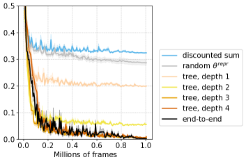
(b)

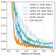
(c)

Figure 3: (a) The illustrative grid world environment. The blue circle denotes the agent and the yellow star denotes the rewarding state. (b) MSE between the learned value function and the true value function in the tree question networks experiment. (c) MSE between the learned value function and the true value function in the random question networks experiment.

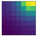
(a)

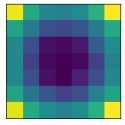
(b)

(c)

(d)

(e)

(f)

Figure 4: Visualization of the learned value functions in the empty room environment. Bright indicates high value and dark indicates low value. (a) The true values. (b) The discounted sum predictions of the touch feature. (c) - (f) The prediction are defined by a full-tree-structured question network regarding the touch feature. The depth of the tree increases from $1$ to $4$ from (c) to (f).

4.1 Benefits of Depth and Action-conditionality: Illustrative Grid World

Although our primary interest (and the focus of subsequent experiments) is learning good policies, in this domain we study policy evaluation because this simpler objective is sufficient to illustrate our points and we can compute and visualize the true value function for comparison. Figure 3(a) shows the environment, a $7$ by $7$ grid surrounded by walls. The observation is a top-down view including the walls. There are $4$ available actions that move the agent horizontally or vertically to an adjacent cell. The agent gets a reward of $1$ upon arriving at the goal cell located in the top row, and $0$ otherwise. This is a continuing environment so achieving the goal does not terminate the interaction. The objective is to learn the state-value function of a random policy which selects each action with equal probability. We used a discount factor of $0.98$.

Specifying a question network requires specifying both the structure and the features. Later we explore random features, but here we use a single hand-crafted touch feature so that every prediction has a clear semantics. touch is $1$ if the agent’s move is blocked by the wall and is $0$ otherwise.

Using the touch feature we constructed two types of question networks. The first type is the discounted sum prediction of touch (we used a discount factor $0.8$) (Figure 2(a)). The second type is a full action-conditional tree of depth $D$. There is only one feature node in the tree which corresponds to the touch feature. Each internal node has $4$ child nodes conditioned on distinct actions. Each prediction node also has a skip edge directly to the feature node (except for the child nodes of the feature node). Figure 2(b) shows an example of a depth-$2$ tree (the caption describes the semantics of some of the predictions). We also compared to a randomly initialized state representation module as a baseline where the state representation was fixed and only the value function weights were learned during training.

Neural Network Architecture. The empty room environment is fully observable and so the state representation module is a feed-forward neural network that maps the current observation $O_{t}$ to a state vector $S_{t}$. It is parameterized by a $3$-layer multi-layer perceptron (MLP) with $64$ units in the first two layers and $32$ units in the third layer. The RL module has one hidden layer with $32$ units and one output head representing the state value. (There is no policy head as the policy was given). The answer network module also has one hidden layer with $32$ units and one output layer. We applied a stop-gradient between the state representation module and the RL module (Figure 1(b)). More implementation details are provided in the Appendix.

Results. We measured the performance by the mean-squared error (MSE) between the learned value function and the true value function across all states. The true value function was obtained by solving a system of linear equations [28]. Figure 3(b) shows the MSE during training. Both the random baseline and the discounted sum prediction target performed poorly. But even a tree question network of depth 1 (i.e., four prediction targets corresponding to the four action conditional predictions of touch after one step) performed much better than these two baselines. Performance increased monotonically with increasing depth until depth $3$ when the MSE matched end-to-end training after $1$ million frames.

Figure 4 shows the different value functions learned by agents with the different prediction tasks. Figure 4(a) visualizes the true values. Figure 4(b) shows the learned value function when the state representations are learned from discounted sum predictions of touch. Its symmetric pattern reflects the symmetry of the grid world and the random policy, but is inconsistent with the asymmetric true values. Figure 4(c) shows the learned value function when the state representations are learned from depth-$1$-tree predictions. It clearly distinguishes $4$ corner states, $4$ groups of states on the boundary, and states in the center area, as this grouping reflects the different prediction targets for these states.

For the answer network module to make accurate predictions of the targets of the question network, the state representation module must map states with the same prediction target to similar representations and states with different targets to different representations. As the question network tree becomes deeper, the agent learns finer state distinctions, until an MSE of $0$ is achieved at depth $3$ (Figure 4(e)).

4.2 Benefits of Random Question Nets: Illustrative Grid World

The previous experiment demonstrated benefits of temporally deeper action-conditonal prediction tasks. But achieving this by creating deeper and deeper full-branching action-conditional trees is not tractable as the number of prediction targets grows exponentially. The previous experiment also used a single feature formulated using domain knowledge; such feature selection is also not scalable. The random generator described in Section 3 provides a method to mitigate both concerns by growing random question networks with random features.

Specifically, we used discount $0.8$, depth $4$, and repeat equal to the number of features for generating random GVFs. Figure 3(c) shows the MSE of different random GVF variants. The performance of random GVFs with touch—that is, random but not necessarily full branching trees of depth $4$—performed as well as touch with a full tree of depth $4$. Random GVFs with a single random feature performed suboptimally; a random feature is likely less discriminative than touch. However, as the number of random features increases, the performance improves, and with $64$ random features, random GVFs match the final performance of touch with a full depth $4$ tree.

The results on the grid world provide preliminary evidence that random deep action-conditional GVFs with many random features can yield good state representations. We next test this conjecture on a set of Atari games, exploring again the benefits of depth and action conditionality.

4.3 Ablation Study of Benefits of Depth and Action Conditionality: Atari

Here we use six Atari games [4] (these six are often used for hyperparameter selection for the Atari benchmark [22]) to compare four different kinds of random GVF question networks: (a) random GVFs in which all predictions are discounted sums of distinct random features (illustrated in Figure 2(a) and denoted rGVFs-discounted-sum in Figure 5); (b) random GVFs in which all predictions are shallow action-conditional predictions, a set of depth-$1$ trees, each for a distinct random feature (denoted rGVFs-shallow in Figure 5); (c) random GVFs without action-conditioning (denoted rGVFs-no-actions in Figure 5); and (d) random GVFs that exploit both action conditionality and depth (illustrated in Figure 2(c) and denoted simply by rGVFs in Figure 5).

Random Features for Atari. The random function $g$ for computing the random features are designed as follows. The $84\times 84$ observation $O_{t}$ is divided into $16$ disjoint $21\times 21$ patches, and a shared random linear function applies to each patch to obtain $16$ random features $g^{1}_{t},g^{2}_{t},\dots,g^{16}_{t}$. Finally, we process these features as described in §3.2.

Neural Network Architecture. We used A2C [22] with a standard neural network architecture for Atari [23] as our base agent. Specifically, the state representation module consists of $3$ convolutional layers. The RL module has one hidden dense layer and two output heads for the policy and the value function respectively. The answer network has one hidden dense layer with $512$ units followed by the output layer. We stopped the gradient from the RL module to the state representation module.

Hyperparameters. The discount factor, depth, and repeat were set to $0.95$, $8$, and $16$ respectively. Thus there are $16+8*16*|\mathcal{A}|$ total predictions. Random GVFs without action-conditioning has the same question network except that no prediction was conditioned on actions. To match the total number of predictions, we used $16+8*16*|\mathcal{A}|$ random features for discounted sum and $8*16$ features for shallow action-conditional predictions. Additional random features were generated by applying more random linear functions to the image patches. The discount factor for discounted sum predictions is also $0.95$. More implementation details are provided in the Appendix.

Results. Figure 5 shows the learning curves in the $6$ Atari games. rGVFs-shallow performed the worst in all the games, providing further evidence for the value of making deep predictions. rGVFs consistently outperformed rGVFs-no-actions, providing evidence that action-conditioning is beneficial. And finally, rGVFs performed better than rGVFs-discounted-sum in $3$ out of $6$ games (large difference in BeamRider and small differences in Breakout and Qbert), was comparable in $2$ the other $3$ games, and performed worse in one—despite using many fewer features than rGVFs-discounted-sum. This suggests that structured deep action-conditional predictions can be more effective than simply making discounted sum predictions about many features.

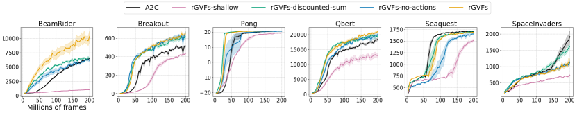
Figure 5: Learning curves of different question networks in six Atari games. x-axis denotes the number of frames and y-axis denotes the episode returns. Each curve is averaged over $5$ independent runs with different random seeds. Shaded area shows the standard error.

4.4 Robustness and Stability

We tested the robustness of rGVFs with respect to its hyperparameters, namely discount, depth, repeat, and number of features. We explored different values for each hyperparameter independently while holding the other hyperparameters fixed to the values we used in the previous experiment. For each hyperparameter, we took $20$ samples uniformly from a wide interval and evaluated rGVFs on Breakout using the sampled value. The results are presented in Figure 6. The lines of best fit (the red lines) in the left two panels indicate a positive correlation between the performance and the depth of the predictions, which is consistent with the previous experiments. Each hyperparameter has a range of values that achieves high performance, indicating that rGVFs are stable and robust to different hyperparameter choices. Additional results in BeamRider and SpaceInvaders are in the Appendix.

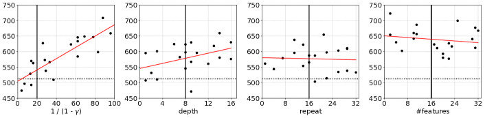
Figure 6: Scatter plots of scores in Breakout obtained by rGVFs with different hyperparameters. x-axis denotes the value of the hyperparameter. y-axis denotes the final game score after training for $200$ million frames. The red line in each panel is the line of best fit. The dotted horizontal lines denote the performance of the end-to-end A2C baseline. The solid vertical lines denotes the values we used in our final experiments.

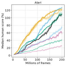
(a)

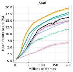
(b)

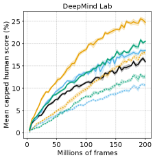
(c)

Figure 7: (a) Median human-normalized score across $49$ Atari games. (b) Mean record-normalized score across $49$ Atari games. (c) Mean capped human-normalized score across $12$ DeepMind Lab environments. In all panels, the x-axis denotes the number of frames. Each dark curve is averaged over $5$ independent runs with different random seeds. The shaded area shows the standard error.

5 Comparison to Baseline Auxiliary Tasks on Atari and DeepMind Lab

In this section, we present the empirical results of comparing the performance of rGVFs against the A2C baseline [22] and three other auxiliary tasks, i.e., multi-horizon value prediction (MHVP) [9], pixel control (PC) [14], and CURL [17]. We conducted the evaluation in $49$ Atari games [4] and $12$ DeepMind Lab environments [2]. It is unclear how to apply CURL to partially observable environments which require long-term memory because CURL is specifically designed to use the stack of recent frames as the inputs. Thus we did not compare to CURL in the DeepMind Lab environments. Our implementation of rGVFs for this experiment is available at https://github.com/Hwhitetooth/random_gvfs.

Atari Implementation. We used the same architecture for rGVFs as in the prior section. For MHVP, we used $10$ value predictions following [9]. Each prediction has a unique discount factor, chosen to be uniform in terms of their effective horizons from $1$ to $100$ ($\{0,1-\frac{1}{10},1-\frac{1}{20},\dots,1-\frac{1}{90}\}$). The architecture for MHVP is the same as rGVFs. For PC, we followed the architecture design and hyperparameters in  [14]. For CURL, we implemented it in our experiment setup by using the code accompanying the paper as a reference . When not stopping gradient from the RL loss, we mixed the RL updates and the answer network updates by scaling the learning rate for the answer network with a coefficient $c$. We searched $c$ in $\{0.1,0.2,0.5,1,2\}$ on the $6$ games in the previous section. $c=1$ worked the best for all methods. More details are in the Appendix.

DeepMind Lab Implementation. We used the same RL module and answer network module as Atari but used a different state representation module to address the partial observability. Specifically, the convolutional layers in the state representation module were followed by a dense layer with $512$ units and a GRU core [5, 6] with $512$ units.

Results. Figure 7(a) and Figure 7(b) shows the results for both the stop-gradient and end-to-end architectures on Atari, comparing to two standard human-normalized score measures (median human-normalized score [23] and mean record-normalized score [13]). When training representations end-to-end through a combined main task and auxiliary task loss, the performance of rGVFs matches or substantially exceeds the three baselines. Although the original paper shows that CURL improves agent performance in the data-efficient regime (i.e., $100K$ interactions in Atari), our results indicate that it hurts the performance in the long run. We conjecture that CURL is held back by failing to capture long-term future in representation learning. Surprisingly, the stop-gradient rGVFs agents outperform the end-to-end A2C baseline, unlike stop-gradient versions of the baseline auxiliary task agents. Figure 7(c) shows the results for both stop-gradient and end-to-end architectures on $12$ DeepMind Lab environments (using mean capped human-normalized scores). Again, rGVFs substantially outperforms both auxiliary task baselines, and the stop-gradient version matches the final performance of the end-to-end A2C. Taken together the results from these $61$ tasks provide substantial evidence that rGVFs drive the learning of good state representations, outperforming auxiliary tasks with fixed hand-crafted semantics.

6 Conclusion and Future Work

In this work we provided evidence that learning how to make random deep action-conditional predictions can drive the learning of good state representations. We explored a rich space of GVFs that can be learned efficiently with TD methods. Our empirical study on the Atari and DeepMind Lab benchmarks shows that learning state representations solely via auxiliary prediction tasks defined by random GVFs outperforms the end-to-end trained A2C baseline. Random GVFs also outperformed pixel control, multi-horizon value prediction, and CURL when being used as part of a combined loss function with the main RL task.

In this work, the question network was sampled before learning and was held fixed during learning. An interesting goal for future research is to find methods that can adapt the question network and discover useful questions during learning. The question networks we studied are limited to discrete actions. It is unclear how to condition a prediction on a continuous action. Thus another future direction to explore is to extend action-conditional predictions to continuous action spaces.

Appendix A Potential Negative Societal Impact

While all AI advances can have potential negative impact on society through their misuse, this work advances our understanding of fundamental questions of interest to RL and at least at this point is far away from potential misuse.

Appendix B Implementation Details

B.1 Experiments on the Empty Room Environment

Neural Network Architecture. The empty room environment is fully observable and so the state representation module is a feed-forward neural network that maps the current observation $O_{t}$ to a state vector $S_{t}$. It is parameterized by a $3$-layer multi-layer perceptron (MLP) with $64$ units in the first two layers and $32$ units in the third layer. The RL module has one hidden layer with $32$ units and one output head representing the state value. (There is no policy head as the policy was given). The answer network module also has one hidden layer with $32$ units and one output layer. ReLU activation is applied after every hidden layer. We applied a stop-gradient between the state representation module and the RL module.

Hyperparameters. Both the value function and the answer network were updated via TD. We used $8$ parallel actors to generate data and updated the parameters every $8$ steps. We used the Adam optimizer [16]. We searched the learning rate in $\{0.01,0.001,0.0001,0.00001\}$ and selected $0.001$ for all agents except the end-to-end agent which used $0.0001$. The value function updates and the answer network updates used two separate optimizers with identical hyperparameters.

B.2 Atari Experiments

Neural Network Architecture. We used A2C [22] with a standard neural network architecture for Atari [23] as our base agent. Specifically, the state representation module consists of $3$ convolutional layers. The first layer has $32$ $8\times 8$ convolutional kernels with a stride of $4$, the second layer has $64$ $4\times 4$ kernels with stride $2$, and the third layer has $64$ $3\times 3$ kernels with stride $1$. The RL module has one dense layer with $512$ units and two output heads for the policy and the value function respectively. The answer network has one hidden dense layer with $512$ units followed by the output layer. ReLU activation is applied after every hidden layer. We stopped the gradient from the RL module to the state representation module.

Hyperparameters. Following convention [23], we used a stack of the latest $4$ frames as the input to the agent, i.e., the input to the state representation module at step $t$ is $(O_{t-3},O_{t-2},O_{t-1},O_{t})$. We used $16$ parallel actors to generate data and updated the agent’s parameters every $20$ steps. The entropy regularization was $0.01$ and the discount factor for the A2C loss was $0.99$. We used the RMSProp optimizer with learning rate $0.0007$, decay $0.99$, and $\epsilon=0.00001$. The RL updates and the answer network updates used two separate optimizers with identical hyperparameters. We used two separate optimizers because the gradients from the RL loss and the gradients from the auxiliary loss may have different statistics. The gradient from the A2C loss was clipped by global norm to $0.5$. The values for the above hyperparameters are taken from a well-tuned open-source implementation of A2C for Atari [8]. These values are used for all methods. When not stopping gradient from the RL loss, we mixed the RL updates and the answer network updates by scaling the learning rate for the answer network with a coefficient $c$. We searched $c$ in $\{0.1,0.2,0.5,1,2\}$ on the $6$ games in the main text. $c=1$ worked the best for both rGVFs and baseline methods. The mixing coefficient was applied to the learning rate for the auxiliary loss because we used separate optimizers.

Baseline Methods. For MHVP, we used $10$ value predictions following [9]. Each prediction has a unique discount factor, chosen to be uniform in terms of their effective horizons from $1$ to $100$ ($\{0,1-\frac{1}{10},1-\frac{1}{20},\dots,1-\frac{1}{90}\}$). The architecture for MHVP is the same as rGVFs. We tried scaling MHVP up to $1024$ predictions in the six Atari games but did not observe any significant performance improvement. Thus we decided to follow the original work. For PC, We followed the architecture design and hyperparameters used in the original work [14]. Specifically, we center-cropped the observation image to $80\times 80$ and used $4\times 4$ patches which resulted in $400$ features. The discount factor was set to $0.9$. The output of the state representation module is first mapped to a $2592$-dimensional vector by a dense layer and then reshaped to a $32\times 9\times 9$ tensor. A deconvolutional layer then maps this $3$D tensor to $|\mathcal{A}|\times 20\times 20$ representing the action-values for each patch. Following [14], we used the dueling architecture [34]. For CURL, we followed the code accompanying the original paper . We used random crop as the sole data augmentation. The $(84,84,4)$ stacked observation was first randomly cropped in to $(80,80,4)$ and then zero-padded to the original size. The output layer of the answer network has $128$ units. The bilinear similarity was computed by a $128\times 128$ matrix whose weights were learned together with the agent parameters. The exponential-moving-average target network used a step size of $0.001$.

B.3 DeepMind Lab Experiments

Neural Network Architecture. For DeepMind Lab, we used the same RL module and answer network module as Atari but used a different state representation module to address the partial observability. Specifically, the convolutional layers in the state representation module were followed by a dense layer with $512$ units and a GRU core [5, 6] with $512$ units.

Hyperparameters. We used $32$ parallel actors to generate data and updated the agent’s parameters every $20$ steps. The discount factor was $0.99$. We searched the entropy regularization in $\{0.001,0.003,0.01,0.03,0.1\}$ for the A2C baseline on explore_goal_locations_small, explore_object_locations_small, and lasertag_three_opponents_small and selected $0.003$. We used the RMSProp optimizer with decay $0.99$ and $\epsilon=10^{-8}$ without tuning. We searched the learning rate in $\{0.00003,0.0001,0.0003,0.001\}$ for the A2C baseline and selected $0.0003$. The gradient from the A2C loss was clipped by global norm to $0.5$. The values for the above hyperparameters are used for all methods. The RL updates and the answer network updates used two separate optimizers with identical hyperparameters. We used two separate optimizers because the gradients from the RL loss and the gradients from the auxiliary loss may have different statistics. For end-to-end (not stop-gradient) agents, we searched the mixing coefficient $c$ in $\{0.1,0.2,0.5,1,2\}$ on explore_goal_locations_small, explore_object_locations_small, and lasertag_three_opponents_small. $c=1$ worked the best for both rGVFs and baseline methods. The mixing coefficient was applied to the learning rate for the auxiliary loss because we used separate optimizers.

B.4 Hardware

Each agent was trained on a single NVIDIA GeForce RTX $2080$ Ti in all of our experiments.

B.5 Computational Cost

Like all auxiliary task methods, the additional computation of the GVF predictions introduces an overhead to the overall training pipeline. In our experiment, we found that the overhead was tiny. rGVFs was only $6\%$ slower than the A2C baseline because the bottleneck was the agent-environment interaction rather than the parameter updates.

Appendix C Pseudocode for The Random Question Network Generator

Algorithm 1 A Random Question Network Generator

  Input: number of features $n_{p}$, discount factor $\gamma$, action set $\mathcal{A}$, depth $D$ and repeat $R$

  Output: a network $G$

  $G\leftarrow$ an empty graph

  $roots\leftarrow$ an empty set

  $leaves\leftarrow$ an empty set

  for $i=1$ to $n_{p}$ do

     create a new feature node $f$ in $G$

     $roots\leftarrow roots\cup\{f\}$

     $leaves\leftarrow leaves\cup\{f\}$

     create a new prediction node $v$ in $G$

     $leaves\leftarrow leaves\cup\{v\}$

     add edge $<v,f,1>$ to $G$

     add edge $<v,v,\gamma>$ to $G$

  end for

  for $d=1$ to $D$ do

     $expanded\leftarrow$ an empty set

     for $a\in A$ do

        $parent\leftarrow$ randomly select $R$ nodes from $leaves$ without replacement

        for $p\in parent$ do

           create a new prediction node $v$ in $G$

           mark $v$ as conditioned on action $a$

           $expanded\leftarrow expanded\cup\{v\}$

           add edge $<v,p,1>$ to $G$

           $f\leftarrow$ randomly select a node from $roots$

           add edge $<v,f,1>$ to $G$

        end for

     end for

     $leaves\leftarrow expanded$

  end for

Appendix D Additional Empirical Results

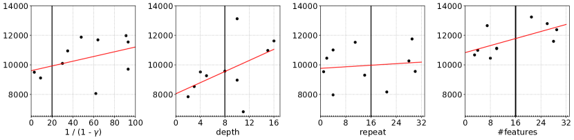
(a)

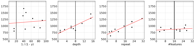
(b)

Figure 8: Scatter plots of scores in (a) BeamRider and (b) SpaceInvaders obtained by rGVFs with different hyperparameters. x-axis denotes the value of the hyperparameter. y-axis denotes the final game score after training for $200$ million frames. The red line in each panel is the line of best fit. The dotted horizontal lines denote the performance of the end-to-end A2C baseline. The solid vertical lines denotes the values we used in our final experiments.

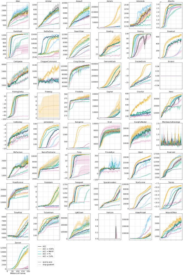
Figure 9: Learning curves in $49$ Atari games. The x-axis denotes the number of frames. Each dark curve is averaged over $5$ independent runs with different random seeds. The shaded area shows the standard error.

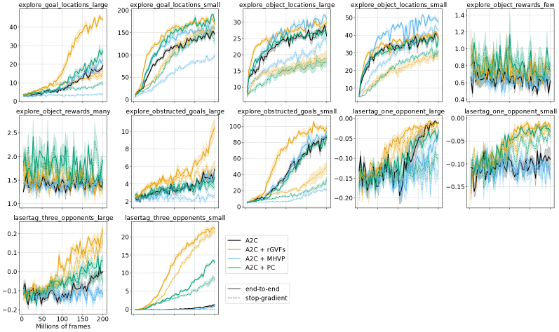
Figure 10: Learning curves in $12$ DeepMind Lab environments. The x-axis denotes the number of frames. Each dark curve is averaged over $5$ independent runs with different random seeds. The shaded area shows the standard error.

References

- [1] Ankesh Anand, Evan Racah, Sherjil Ozair, Yoshua Bengio, Marc-Alexandre Côté, and R. Devon Hjelm. Unsupervised state representation learning in atari. In Hanna M. Wallach, Hugo Larochelle, Alina Beygelzimer, Florence d’Alché-Buc, Emily B. Fox, and Roman Garnett, editors, Advances in Neural Information Processing Systems 32: Annual Conference on Neural Information Processing Systems 2019, NeurIPS 2019, December 8-14, 2019, Vancouver, BC, Canada, pages 8766–8779, 2019.
- [2] Charles Beattie, Joel Z. Leibo, Denis Teplyashin, Tom Ward, Marcus Wainwright, Heinrich Küttler, Andrew Lefrancq, Simon Green, Víctor Valdés, Amir Sadik, Julian Schrittwieser, Keith Anderson, Sarah York, Max Cant, Adam Cain, Adrian Bolton, Stephen Gaffney, Helen King, Demis Hassabis, Shane Legg, and Stig Petersen. Deepmind lab. CoRR, abs/1612.03801, 2016.
- [3] Marc G. Bellemare, Will Dabney, Robert Dadashi, Adrien Ali Taïga, Pablo Samuel Castro, Nicolas Le Roux, Dale Schuurmans, Tor Lattimore, and Clare Lyle. A geometric perspective on optimal representations for reinforcement learning. In Hanna M. Wallach, Hugo Larochelle, Alina Beygelzimer, Florence d’Alché-Buc, Emily B. Fox, and Roman Garnett, editors, Advances in Neural Information Processing Systems 32: Annual Conference on Neural Information Processing Systems 2019, NeurIPS 2019, December 8-14, 2019, Vancouver, BC, Canada, pages 4360–4371, 2019.
- [4] Marc G. Bellemare, Yavar Naddaf, Joel Veness, and Michael Bowling. The arcade learning environment: An evaluation platform for general agents. J. Artif. Intell. Res., 47:253–279, 2013.
- [5] Kyunghyun Cho, Bart van Merrienboer, Dzmitry Bahdanau, and Yoshua Bengio. On the properties of neural machine translation: Encoder-decoder approaches. In Dekai Wu, Marine Carpuat, Xavier Carreras, and Eva Maria Vecchi, editors, Proceedings of SSST@EMNLP 2014, Eighth Workshop on Syntax, Semantics and Structure in Statistical Translation, Doha, Qatar, 25 October 2014, pages 103–111. Association for Computational Linguistics, 2014.
- [6] Junyoung Chung, Çaglar Gülçehre, KyungHyun Cho, and Yoshua Bengio. Empirical evaluation of gated recurrent neural networks on sequence modeling. CoRR, abs/1412.3555, 2014.
- [7] Will Dabney, André Barreto, Mark Rowland, Robert Dadashi, John Quan, Marc G. Bellemare, and David Silver. The value-improvement path: Towards better representations for reinforcement learning. CoRR, abs/2006.02243, 2020.
- [8] Prafulla Dhariwal, Christopher Hesse, Oleg Klimov, Alex Nichol, Matthias Plappert, Alec Radford, John Schulman, Szymon Sidor, Yuhuai Wu, and Peter Zhokhov. Openai baselines. https://github.com/openai/baselines, 2017.
- [9] William Fedus, Carles Gelada, Yoshua Bengio, Marc G. Bellemare, and Hugo Larochelle. Hyperbolic discounting and learning over multiple horizons. CoRR, abs/1902.06865, 2019.
- [10] Karol Gregor, Danilo Jimenez Rezende, Frederic Besse, Yan Wu, Hamza Merzic, and Aäron van den Oord. Shaping belief states with generative environment models for RL. In Hanna M. Wallach, Hugo Larochelle, Alina Beygelzimer, Florence d’Alché-Buc, Emily B. Fox, and Roman Garnett, editors, Advances in Neural Information Processing Systems 32: Annual Conference on Neural Information Processing Systems 2019, NeurIPS 2019, December 8-14, 2019, Vancouver, BC, Canada, pages 13475–13487, 2019.
- [11] Zhaohan Daniel Guo, Mohammad Gheshlaghi Azar, Bilal Piot, Bernardo A. Pires, Toby Pohlen, and Rémi Munos. Neural predictive belief representations. CoRR, abs/1811.06407, 2018.
- [12] Zhaohan Daniel Guo, Bernardo Ávila Pires, Bilal Piot, Jean-Bastien Grill, Florent Altché, Rémi Munos, and Mohammad Gheshlaghi Azar. Bootstrap latent-predictive representations for multitask reinforcement learning. In Proceedings of the 37th International Conference on Machine Learning, ICML 2020, 13-18 July 2020, Virtual Event, volume 119 of Proceedings of Machine Learning Research, pages 3875–3886. PMLR, 2020.
- [13] Danijar Hafner, Timothy P. Lillicrap, Mohammad Norouzi, and Jimmy Ba. Mastering atari with discrete world models. CoRR, abs/2010.02193, 2020.
- [14] Max Jaderberg, Volodymyr Mnih, Wojciech Marian Czarnecki, Tom Schaul, Joel Z. Leibo, David Silver, and Koray Kavukcuoglu. Reinforcement learning with unsupervised auxiliary tasks. In 5th International Conference on Learning Representations, ICLR 2017, Toulon, France, April 24-26, 2017, Conference Track Proceedings. OpenReview.net, 2017.
- [15] Bilal Kartal, Pablo Hernandez-Leal, and Matthew E. Taylor. Terminal prediction as an auxiliary task for deep reinforcement learning. In Gillian Smith and Levi Lelis, editors, Proceedings of the Fifteenth AAAI Conference on Artificial Intelligence and Interactive Digital Entertainment, AIIDE 2019, October 8-12, 2019, Atlanta, Georgia, USA, pages 38–44. AAAI Press, 2019.
- [16] Diederik P. Kingma and Jimmy Ba. Adam: A method for stochastic optimization. In Yoshua Bengio and Yann LeCun, editors, 3rd International Conference on Learning Representations, ICLR 2015, San Diego, CA, USA, May 7-9, 2015, Conference Track Proceedings, 2015.
- [17] Michael Laskin, Aravind Srinivas, and Pieter Abbeel. CURL: contrastive unsupervised representations for reinforcement learning. In Proceedings of the 37th International Conference on Machine Learning, ICML 2020, 13-18 July 2020, Virtual Event, volume 119 of Proceedings of Machine Learning Research, pages 5639–5650. PMLR, 2020.
- [18] Kuang-Huei Lee, Ian Fischer, Anthony Liu, Yijie Guo, Honglak Lee, John Canny, and Sergio Guadarrama. Predictive information accelerates learning in RL. In Hugo Larochelle, Marc’Aurelio Ranzato, Raia Hadsell, Maria-Florina Balcan, and Hsuan-Tien Lin, editors, Advances in Neural Information Processing Systems 33: Annual Conference on Neural Information Processing Systems 2020, NeurIPS 2020, December 6-12, 2020, virtual, 2020.
- [19] Michael L. Littman, Richard S. Sutton, and Satinder Singh. Predictive representations of state. In Thomas G. Dietterich, Suzanna Becker, and Zoubin Ghahramani, editors, Advances in Neural Information Processing Systems 14 [Neural Information Processing Systems: Natural and Synthetic, NIPS 2001, December 3-8, 2001, Vancouver, British Columbia, Canada], pages 1555–1561. MIT Press, 2001.
- [20] Clare Lyle, Mark Rowland, Georg Ostrovski, and Will Dabney. On the effect of auxiliary tasks on representation dynamics. In Arindam Banerjee and Kenji Fukumizu, editors, The 24th International Conference on Artificial Intelligence and Statistics, AISTATS 2021, April 13-15, 2021, Virtual Event, volume 130 of Proceedings of Machine Learning Research, pages 1–9. PMLR, 2021.
- [21] Bogdan Mazoure, Remi Tachet des Combes, Thang Doan, Philip Bachman, and R. Devon Hjelm. Deep reinforcement and infomax learning. In Hugo Larochelle, Marc’Aurelio Ranzato, Raia Hadsell, Maria-Florina Balcan, and Hsuan-Tien Lin, editors, Advances in Neural Information Processing Systems 33: Annual Conference on Neural Information Processing Systems 2020, NeurIPS 2020, December 6-12, 2020, virtual, 2020.
- [22] Volodymyr Mnih, Adrià Puigdomènech Badia, Mehdi Mirza, Alex Graves, Timothy P. Lillicrap, Tim Harley, David Silver, and Koray Kavukcuoglu. Asynchronous methods for deep reinforcement learning. In Maria-Florina Balcan and Kilian Q. Weinberger, editors, Proceedings of the 33nd International Conference on Machine Learning, ICML 2016, New York City, NY, USA, June 19-24, 2016, volume 48 of JMLR Workshop and Conference Proceedings, pages 1928–1937. JMLR.org, 2016.
- [23] Volodymyr Mnih, Koray Kavukcuoglu, David Silver, Andrei A. Rusu, Joel Veness, Marc G. Bellemare, Alex Graves, Martin A. Riedmiller, Andreas Fidjeland, Georg Ostrovski, Stig Petersen, Charles Beattie, Amir Sadik, Ioannis Antonoglou, Helen King, Dharshan Kumaran, Daan Wierstra, Shane Legg, and Demis Hassabis. Human-level control through deep reinforcement learning. Nat., 518(7540):529–533, 2015.
- [24] Matthew Schlegel, Andrew Jacobsen, Zaheer Abbas, Andrew Patterson, Adam White, and Martha White. General value function networks. J. Artif. Intell. Res., 70:497–543, 2021.
- [25] Max Schwarzer, Ankesh Anand, Rishab Goel, R Devon Hjelm, Aaron Courville, and Philip Bachman. Data-efficient reinforcement learning with self-predictive representations. arXiv preprint arXiv:2007.05929, 2020.
- [26] Satinder Singh, Michael R. James, and Matthew R. Rudary. Predictive state representations: A new theory for modeling dynamical systems. In David Maxwell Chickering and Joseph Y. Halpern, editors, UAI ’04, Proceedings of the 20th Conference in Uncertainty in Artificial Intelligence, Banff, Canada, July 7-11, 2004, pages 512–518. AUAI Press, 2004.
- [27] Adam Stooke, Kimin Lee, Pieter Abbeel, and Michael Laskin. Decoupling representation learning from reinforcement learning. In Marina Meila and Tong Zhang, editors, Proceedings of the 38th International Conference on Machine Learning, ICML 2021, 18-24 July 2021, Virtual Event, volume 139 of Proceedings of Machine Learning Research, pages 9870–9879. PMLR, 2021.
- [28] Richard S Sutton and Andrew G Barto. Reinforcement learning: An introduction. MIT press, 2018.
- [29] Richard S. Sutton, Joseph Modayil, Michael Delp, Thomas Degris, Patrick M. Pilarski, Adam White, and Doina Precup. Horde: a scalable real-time architecture for learning knowledge from unsupervised sensorimotor interaction. In Liz Sonenberg, Peter Stone, Kagan Tumer, and Pinar Yolum, editors, 10th International Conference on Autonomous Agents and Multiagent Systems (AAMAS 2011), Taipei, Taiwan, May 2-6, 2011, Volume 1-3, pages 761–768. IFAAMAS, 2011.
- [30] Richard S. Sutton, Eddie J. Rafols, and Anna Koop. Temporal abstraction in temporal-difference networks. In Advances in Neural Information Processing Systems 18 [Neural Information Processing Systems, NIPS 2005, December 5-8, 2005, Vancouver, British Columbia, Canada], pages 1313–1320, 2005.
- [31] Richard S. Sutton and Brian Tanner. Temporal-difference networks. In Advances in Neural Information Processing Systems 17 [Neural Information Processing Systems, NIPS 2004, December 13-18, 2004, Vancouver, British Columbia, Canada], pages 1377–1384, 2004.
- [32] Aäron van den Oord, Yazhe Li, and Oriol Vinyals. Representation learning with contrastive predictive coding. CoRR, abs/1807.03748, 2018.
- [33] Vivek Veeriah, Matteo Hessel, Zhongwen Xu, Janarthanan Rajendran, Richard L. Lewis, Junhyuk Oh, Hado van Hasselt, David Silver, and Satinder Singh. Discovery of useful questions as auxiliary tasks. In Hanna M. Wallach, Hugo Larochelle, Alina Beygelzimer, Florence d’Alché-Buc, Emily B. Fox, and Roman Garnett, editors, Advances in Neural Information Processing Systems 32: Annual Conference on Neural Information Processing Systems 2019, NeurIPS 2019, December 8-14, 2019, Vancouver, BC, Canada, pages 9306–9317, 2019.
- [34] Ziyu Wang, Tom Schaul, Matteo Hessel, Hado van Hasselt, Marc Lanctot, and Nando de Freitas. Dueling network architectures for deep reinforcement learning. In Maria-Florina Balcan and Kilian Q. Weinberger, editors, Proceedings of the 33nd International Conference on Machine Learning, ICML 2016, New York City, NY, USA, June 19-24, 2016, volume 48 of JMLR Workshop and Conference Proceedings, pages 1995–2003. JMLR.org, 2016.