Binet’s factorial series and extensions to Laplace transforms

Abstract

We investigate a generalization of Binet’s factorial series in the parameter $\alpha$

$$\mu\left(z\right)=\sum_{m=1}^{\infty}\frac{b_{m}\left(\alpha\right)}{\prod_{k=0}^{m-1}(z+\alpha+k)}$$

due to Gilbert, for the Binet function

$$\mu\left(z\right)=\log\Gamma\left(z\right)-\left(z-\frac{1}{2}\right)\log z+z-\frac{1}{2}\log\left(2\pi\right)$$

After a review of the Binet function $\mu\left(z\right)$ and Gilbert’s investigations of $\mu\left(z\right)$, several properties of the Binet polynomials $b_{m}\left(\alpha\right)$ are presented. We compare Gilbert’s generalized factorial series with Stirling’s asymptotic expansion and demonstrate by a numerical example that, with a same number of terms evaluated, the Gilbert generalized factorial series with an optimized value of $\alpha$ can beat the best possible accuracy of Stirling’s expansion. Finally, we extend Binet’s method to factorial series of Laplace transforms.

1 Introduction

In his truly comprehensive “memoir” [2, Section 3, p. 223] in 1839, Jacques Binet defines his function $\mu\left(z\right)$ in relation to the Gamma function $\Gamma\left(z\right)$ as

$$\mu\left(z\right)=\log\Gamma\left(z\right)-\left(z-\frac{1}{2}\right)\log z+z-\frac{1}{2}\log\left(2\pi\right)$$ (1)

Binet has derived two integral representations of his function [32, p. 248-251], [22, p. 211-217], for $\operatorname{Re}\left(z\right)>0$,

$$\mu\left(z\right)=2\int_{0}^{\infty}\frac{\arctan\left(\frac{t}{z}\right)}{e^{2\pi t}-1}dt$$ (2)

and

$$\mu\left(z\right)=\frac{1}{2}\int_{0}^{\infty}\frac{e^{-zt}}{t}\left(\frac{1+e^{-t}}{1-e^{-t}}-\frac{2}{t}\right)dt$$ (3)

There exist more representations of $\mu\left(z\right)$, but here we merely concentrate on elegant, converging factorial series for $\operatorname{Re}\left(z\right)>0$ due to Binet in [2, p. 234],

$$\mu\left(z\right)=\sum_{m=1}^{\infty}\frac{\beta_{m}}{\left(z+1\right)\left(z+2\right)\cdots\left(z+m\right)}$$ (6)

where the coefficients are

$$\beta_{m}=\frac{1}{m}\int_{0}^{1}\left(u-\frac{1}{2}\right)u\left(u+1\right)\cdots\left(u+m-1\right)du$$ (7)

Explicitly, $\beta_{1}=\beta_{2}=\frac{1}{12}$, $\beta_{3}=\frac{59}{360}$, $\beta_{4}=\frac{29}{60}$, $\beta_{5}=\frac{533}{280}$, $\beta_{6}=\frac{1577}{168}$, $\beta_{7}=\frac{280361}{5040}$, $\beta_{8}=\frac{69311}{180}$, and $\beta_{m}$ is positive and rapidly increasing in $m$. Nearly at the end of his memoir and somewhat hidden, Binet [2, p. 342] has given a second factorial series (38), that is rederived slightly differently in Theorem 1 in Section 3.2 and generalized to Laplace transforms in Section 8.2.

Recently, Nemes [17, Theorem 2.1] has generalized Binet’s expansion (6), for $0\leq a\leq 1$ and $\operatorname{Re}\left(z\right)>0$,

$$\log\Gamma\left(z+a\right)=\left(z+a-\frac{1}{2}\right)\log z-z+\frac{1}{2}\log\left(2\pi\right)+\sum_{m=1}^{\infty}\frac{c_{m}\left(a\right)}{\left(z+1\right)\left(z+2\right)\cdots\left(z+m\right)}$$ (8)

where

$$c_{m}\left(a\right)=\frac{1}{m}\int_{0}^{1}\left(u+a-\frac{1}{2}\right)u\left(u+1\right)\cdots\left(u+m-1\right)du-\frac{1}{m}\int_{0}^{a}\prod_{j=0}^{m-1}\left(u-a+1+j\right)du$$ (9)

Clearly, if $a=0$, we retrieve Binet’s first factorial expansion (6) and coefficients $\beta_{m}$ in (7). Nemes’ expansion (8), expressed in terms of Binet’s function $\mu\left(z\right)$ with the definition (1),

$$\mu\left(z\right)=\left(z-\frac{1}{2}\right)\log\frac{z-a}{z}+a+\sum_{m=1}^{\infty}\frac{c_{m}\left(a\right)}{\prod_{k=1}^{m}(z-a+k)}$$

bears resemblance to

$$\mu\left(z\right)=\sum_{m=1}^{\infty}\frac{b_{m}\left(\alpha\right)}{\prod_{k=0}^{m-1}(z+\alpha+k)}$$ (10)

in our main Theorem 3, where the coefficients $b_{m}\left(\alpha\right)$ are called Binet polynomials, to honour Jacques Binet. Much earlier, Hermite [14] has deduced the corresponding generalized Stirling asymptotic expansion

$$\log\Gamma\left(z+a\right)\simeq\left(z+a-\frac{1}{2}\right)\log z-z+\frac{1}{2}\log\left(2\pi\right)+\sum_{k=1}^{K}\frac{\left(-1\right)^{k-1}B_{k+1}\left(a\right)}{k\left(k+1\right)z^{k}}$$ (11)

in terms of the Bernoulli polynomials $B_{n}\left(a\right)$ that reduces for $a=0$ to Stirling’s original asymptotic series (28). Starting from a complex integral (24) for Binet’s function $\mu\left(z\right)$, Stirling’s asymptotic series (28) is derived in Section 2.4, where also the meaning of the upper bound $K$ is explained. Section 2.5 presents the convergent companion (31) of Stirling’s divergent series (if $K\rightarrow\infty$ in (28)).

The main motivation that led to this article is twofold. Originally, I was confused about Binet’s achievements: he derived two different factorial expansions (6) and (38) for the same function $\mu\left(z\right)$. While I thought initially that one of them must be wrong, I discovered later with (10) that infinitely many different factorial series exist. However, Gilbert [8] has anticipated me about 150 years earlier. The second motivation was my unbelief that Stirling’s asymptotic but divergent expansion seems unbeatable in performance for some optimal, finite $K$.

Rediscoveries seem to appear frequently in mathematics. In earlier versions, I wrote that “our main result is the demonstration that there exist infinitely many different factorial expansions in a complex parameter $\alpha$ for Binet’s function $\mu\left(z\right)$”. After Gergő Nemes informed me in January 2023 about Gilbert’s investigations in [8], I have reoriented the article by integrating the beautiful discoveries of predessors with my own findings in Theorem 3 (Section 5) and for Laplace transforms in Theorem 4 (Section 8.3). My approach is different from Gilbert’s and an integrated presentation provides a broader view on Binet’s function $\mu\left(z\right)$. For $\alpha=1$ in (10), we recover Binet’s first factorial series (6) with $b_{m}\left(1\right)=\beta_{m}$ in (7), while $\alpha=0$ in (10) corresponds to Binet’s second factorial series (38) with $b_{m}\left(0\right)=c_{m}$ in (39). Interestingly, the $\alpha=1$ factorial series has all positive coefficients and any truncation thus lower bounds Binet’s function $\mu\left(z\right)$, while the $\alpha=0$ factorial series is shown in Theorem 2 to possess coefficients $c_{m}<0$ for $m>2$. Thus, a truncation of (38) upper bounds $\mu\left(z\right)$. For $\alpha$ around $\frac{1}{10}$, which is close to the largest zero of the Binet polynomial $b_{m}\left(\alpha\right)$, numerical computations exhibit the fastest convergence. With the same number $K$ of terms evaluated, the variant $\alpha=0$ is more accurate than the variant $\alpha=1$. Perhaps, the slower convergence of Binet’s expansion (6) has led to its omission in handbooks of functions, like Abramowitz & Stegun [1] nor in its successor by Olver et al. [19].

We will first discuss the main properties of Binet’s function $\mu\left(z\right)$ in Section 2.1 and the deductions from the complex integral (24) in Section 2.3, before we review parts of Binet’s great treatise. In section 3.1, we sketch Binet’s route towards his first factorial series (6), that is covered in the literature (see e.g. [32, p. 253], [20, p. 30]). Binet’s second factorial series, that I have not found in later works, is derived in more detail in subsection 3.2, also because I believe that, being the case $\alpha=0$ in (10), it is slightly more important than his first series (6) corresponding to $\alpha=1$. Moreover, Binet’s method towards his second factorial series, which is a recipe in five steps, enables a far reaching generalization to Laplace transforms as explained in Section 8. Section 4 reviews Gilbert’s remarkable investigations in [8]. I have slightly generalized in Section 4.2 his derivation of a generalized factorial series in (53) for Binet’s function $\mu\left(z\right)$. Section 5 presents my derivation of Gilbert’s generalized factorial series for $p=1$ in (53) and properties of its coefficients that I have called the Binet polynomial $b_{m}\left(\alpha\right)$. Factorial expansions for the derivatives $\frac{d^{n}\mu\left(z\right)}{dz^{n}}$ are derived in Section 6 and applied to the digamma and polygamma function. In particular for the digamma function $\psi\left(z\right)=\frac{\Gamma^{\prime}\left(z\right)}{\Gamma\left(z\right)}$, we thus add a convergent series (75) to its asymptotic counterpart (76). Section 7 discusses and compares, with a same number of terms, the accuracy of Stirling’s asymptotic expansion and the best possible that can be attained by the generalized Binet factorial expansion. The commonly accepted belief about the superiority of Stirling’s asymptotic expansion is demonstrated and plotted in Fig. 1. However, at the zeros of the Binet polynomial $b_{m}\left(\alpha\right)$, the accuracy of the generalized Binet factorial expansion (10) improves considerably as drawn in Fig. 2. By a numerical example, we show that Stirling’s series accuracy is not always better than a factorial series (with a same number of terms)! In other words, the generalized Binet expansion (10) can be optimized with respect to the “free” parameter $\alpha$ to achieve, at least, a comparable accuracy with a same computational effort. Perhaps, this observation deserves to list the generalized Binet factorial expansion (10) in handbooks of functions.

Computations are deferred to the appendices in order to enhance the readability and focus on the essential parts.

2 Binet’s function $\mu\left(z\right)$

2.1 Properties deduced from the definition (1)

The definition (1) of Binet’s function $\mu\left(z\right)$ directly shows, for a positive integer $z=n$, that

$$\mu\left(n\right)=n+\log\left(n-1\right)!-\left(n-\frac{1}{2}\right)\log\left(n\right)-\frac{1}{2}\log\left(2\pi\right)$$

The sequence $\mu\left(1\right)\simeq 0.0811$, $\mu\left(2\right)\simeq 0.0413$, $\mu\left(3\right)\simeq 0.0277$, $\mu\left(4\right)\simeq 0.0208$, $\mu\left(5\right)\simeq 0.0166$,…, $\mu\left(10\right)\simeq 0.0083$ demonstrates the slow decay roughly as $\mu\left(n\right)\approx\frac{1}{12n}$. The precise decay is given in (80) below.

Maximum at real, positive values of $z$. Binet’s integral (3) can be rewritten as a Laplace transform

$$\mu\left(z\right)=\int_{0}^{\infty}\frac{e^{-zt}}{t}\left(\frac{1}{e^{t}-1}-\frac{1}{t}+\frac{1}{2}\right)dt$$ (12)

where $0\leq\frac{1}{e^{t}-1}-\frac{1}{t}+\frac{1}{2}\leq\frac{1}{2}$ for real, non-negative $t$. Since the integrand is positive for real $z=x>0$, we observe that $\mu\left(x\right)>0$ for real, positive $x$. In addition, for a complex number $z=x+iy$, the above integral shows that $\mu\left(z\right)$ is analytic for $\operatorname{Re}\left(z\right)>0$ and that

$$\left|\mu\left(z\right)\right|\leq\int_{0}^{\infty}\frac{e^{-xt}}{t}\left(\frac{1}{e^{t}-1}-\frac{1}{t}+\frac{1}{2}\right)dt=\mu\left(x\right)$$

In other words, the maximum absolute value of Binet’s function $\mu\left(z\right)$ for $\operatorname{Re}\left(z\right)>0$ is attained at the positive real axis. Moreover, $\mu\left(x\right)$ strictly decreases with $x=\operatorname{Re}\left(z\right)$. Another rather straightforward bound is

$$\left|\mu\left(z\right)\right|\leq\max_{0\leq t}\frac{1}{t}\left(\frac{1}{e^{t}-1}-\frac{1}{t}+\frac{1}{2}\right)\int_{0}^{\infty}e^{-xt}dt=\frac{1}{x}\max_{0\leq t}\frac{1}{t}\left(\frac{1}{e^{t}-1}-\frac{1}{t}+\frac{1}{2}\right)$$

Since the maximum occurs at $t=0$, the generating function of the Bernoulli numbers $B_{n}$

$$\frac{1\,}{e^{t}-1}=\frac{1}{t}-\frac{1}{2}+\sum_{n=1}^{\infty}B_{2n}\,\frac{t^{2n-1}}{(2n)!}\hskip 28.45274pt\text{for }\left|t\right|\leq 2\pi$$ (13)

illustrates that $\max_{0\leq t}\frac{1}{t}\left(\frac{1}{e^{t}-1}-\frac{1}{t}+\frac{1}{2}\right)=\frac{B_{2}}{2}=\frac{1}{12}$. Hence, for $x=\operatorname{Re}\left(z\right)>0$, we find [32, p. 249]

$$\left|\mu\left(z\right)\right|\leq\mu\left(x\right)\leq\frac{1}{12x}$$ (14)

Difference $\mu\left(z+1\right)-\mu\left(z\right)$. Binet’s definition (1)

$$\mu\left(z\right)=\log\Gamma\left(z\right)-\left(z-\frac{1}{2}\right)\log z+z-\frac{1}{2}\log\left(2\pi\right)$$

illustrates that the complex conjugate $\mu^{\ast}\left(z\right)=\mu\left(z^{\ast}\right)$, by the reflection principle [26, p. 155]. The functional equation of the Gamma function $\Gamma\left(z+1\right)=z\Gamma\left(z\right)$ leads to

$$\mu\left(z+1\right)=\log\Gamma\left(z\right)+\log z-\left(z+\frac{1}{2}\right)\log\left(z+1\right)+z+1-\frac{1}{2}\log\left(2\pi\right)$$

The forward difference $\Delta\mu(z)=\mu\left(z+1\right)-\mu\left(z\right)$ equals

$$\mu\left(z+1\right)-\mu\left(z\right)=\left(z+\frac{1}{2}\right)\log\frac{z}{z+1}+1$$ (15)

which is valid for any complex $z$, except at the negative real axis that is a branch cut for $\mu\left(z\right)$. In particular, around $z=0$, the forward difference (15) shows, with $\mu\left(1\right)=1-\frac{1}{2}\log\left(2\pi\right)$, that

$$\mu\left(z\right)\sim-\frac{1}{2}\log z-\frac{1}{2}\log\left(2\pi\right)$$ (16)

illustrating that Binet’s function $\mu\left(z\right)$ possesses a logarithmic singularity at $z=0$.

Erdelyi et al. [6, p. 24] deduce from Gauss’s multiplication formula that

$$\int_{z}^{z+1}\log\Gamma\left(t\right)dt=z\log z-z+\frac{1}{2}\log\left(2\pi\right)$$

which we rewrite with the definition (1) as

$$\int_{z}^{z+1}\mu\left(t\right)dt=\frac{1}{2}\left(z\left(z+1\right)\log\left(\frac{z}{z+1}\right)+z+\frac{1}{2}\right)$$ (17)

Differentiation of (17) with respect to $z$ again leads to the forward difference (15). For $z=0$ in (17), we find $\int_{0}^{1}\mu\left(t\right)dt=\frac{1}{4}$.

Gudderman’s series. If we replace $z$ by $z+k$ in the forward difference (15) and change the sign, then (15) becomes $\mu\left(z+k\right)-\mu\left(z+k+1\right)=\left(z+k+\frac{1}{2}\right)\log\left(1+\frac{1}{z+k}\right)-1$. Summing over integer $k$ results in a telescoping series $\sum_{k=0}^{K}\left\{\mu\left(z+k\right)-\mu\left(z+k+1\right)\right\}=\mu\left(z\right)-\mu\left(z+K+1\right)$ leading to

$$\mu\left(z\right)-\mu\left(z+K+1\right)=\sum_{k=0}^{K}\left\{\left(z+k+\frac{1}{2}\right)\log\left(1+\frac{1}{z+k}\right)-1\right\}$$

When $K$ tends to infinity, the bound (14) shows that $\lim_{K\rightarrow\infty}\mu\left(z+K+1\right)=0$ and we obtain Gudermann’s series [11]

$$\mu\left(z\right)=\sum_{k=0}^{\infty}\left\{\left(z+k+\frac{1}{2}\right)\log\left(1+\frac{1}{z+k}\right)-1\right\}$$ (18)

Reflection formula of Binet’s function $\mu\left(z\right)$. We replace $z\rightarrow 1-z$ in Binet’s definition (1)

$$\mu\left(1-z\right)=\log\Gamma\left(1-z\right)-\left(\frac{1}{2}-z\right)\log\left(1-z\right)-z+1-\frac{1}{2}\log\left(2\pi\right)$$

which added to $\mu\left(z\right)$ in (1), yields

$$\mu\left(z\right)+\mu\left(1-z\right)=\log\left(\Gamma\left(z\right)\Gamma\left(1-z\right)\right)-\left(z-\frac{1}{2}\right)\log\frac{z}{1-z}+1-\log\left(2\pi\right)$$

After invoking the reflection formula of the Gamma function $\Gamma\left(z\right)\Gamma\left(1-z\right)=\frac{\pi}{\sin\pi z}$, we find the corresponding “reflection” formula for Binet’s function

$$\mu\left(1-z\right)=1-\mu\left(z\right)-\log\left(2\sin\pi z\right)-\left(z-\frac{1}{2}\right)\log\frac{z}{1-z}$$ (19)

which is valid for any complex number $z=x+iy$, with the exception of the negative real axis and odd integers $x=2n+1$ with $n\in\mathbb{Z}$ at any $y$. Since $\mu\left(z\right)$ is analytic for $\operatorname{Re}\left(z\right)>0$, the Binet reflection formula (19) illustrates that Binet’s function $\mu\left(z\right)$ has only logarithmic singularities at negative integers $z=-k$ (with $k\in\mathbb{N}$) including $z=0$, as shown in (16).

Duplication and multiplication formula for $\mu\left(z\right)$. Combining the duplication formula $\Gamma\left(2z\right)=\frac{2^{2z-1}}{\sqrt{\pi}}\Gamma\left(z\right)\Gamma\left(z+\frac{1}{2}\right)$ in [1, 6.1.18] for the Gamma function $\Gamma\left(z\right)$ and the definition (1) of Binet’s function $\mu\left(z\right)$ leads to

$$\mu\left(2z\right)=\mu\left(z+\frac{1}{2}\right)+\mu\left(z\right)+z\log\left(1+\frac{1}{2z}\right)-\frac{1}{2}$$ (20)

which is generalized by Gauss’s multiplication formula $\Gamma\left(nz\right)=\left(2\pi\right)^{\frac{1}{2}\left(1-n\right)}n^{nz-\frac{1}{2}}{\displaystyle\prod\limits_{k=0}^{n-1}}\Gamma\left(z+\frac{k}{n}\right)$ in [1, 6.1.20] as

$$\mu\left(nz\right)=\mu\left(z\right)+\sum_{k=1}^{n-1}\mu\left(z+\frac{k}{n}\right)+\sum_{k=1}^{n-1}\left(z+\frac{k}{n}-\frac{1}{2}\right)\log\left(z+\frac{k}{n}\right)-\left(n-1\right)\left(\frac{1}{2}+z\log z\right)$$ (21)

After choosing $z=\frac{1}{n}$ in (21), we find for $n\geq 2$

$$\mu\left(\frac{1}{n}\right)=-\sum_{k=1}^{n-2}\mu\left(\frac{k+1}{n}\right)-\sum_{k=1}^{n-2}\left(\frac{k+1}{n}-\frac{1}{2}\right)\log\left(\frac{k+1}{n}\right)+\left(n-1\right)\left(\frac{1}{2}-\frac{1}{n}\log n\right)$$

For example, for $n=2$, we obtain $\mu\left(\frac{1}{2}\right)=\frac{1}{2}\left(1-\log 2\right)\simeq 0.1534$ but, for $n=3$, $\mu\left(\frac{1}{3}\right)=1-\mu\left(\frac{2}{3}\right)-\frac{1}{6}\log\left(2\right)-\frac{1}{2}\log\left(3\right)$, which is also immediate from Binet’s reflection formula (19). The duplication formula (20) yields a closed expression for $z=n+\frac{1}{2}$ with integer $n\geq 1$,

$$\mu\left(n+\frac{1}{2}\right)=\sum_{k=n}^{2n-1}\log k-n\left(\log\left(4n+2\right)-1\right)+\frac{1}{2}\left(\log\left(2\right)+1\right)$$

2.2 Gilbert’s infinite product for $\Gamma\left(z\right)$

Gilbert [8, art. 3] further investigates Gudermann’s series (18). After remarking that

$$\sum_{k=0}^{K}\left(z+k+\frac{1}{2}\right)\log\left(1+\frac{1}{z+k}\right) =\sum_{k=0}^{K}\left(z+k+\frac{1}{2}\right)\left(\log\left(z+k+1\right)-\log\left(z+k\right)\right)$$

$$=\sum_{k=1}^{K+1}\left(z+k-\frac{1}{2}\right)\log\left(z+k\right)-\sum_{k=0}^{K}\left(z+k+\frac{1}{2}\right)\log\left(z+k\right)$$

and reworking the (telescoping) sums,

$$\sum_{k=0}^{K}\left(z+k+\frac{1}{2}\right)\log\left(1+\frac{1}{z+k}\right)=\left(z+K+\frac{1}{2}\right)\log\left(z+K+1\right)-\left(z+\frac{1}{2}\right)\log\left(z\right)-\sum_{k=1}^{K}\log\left(z+k\right)$$

Gilbert [8, art. 3] finds

$$\mu\left(z\right)-\mu\left(z+K+1\right) =\sum_{k=0}^{K}\left\{\left(z+k+\frac{1}{2}\right)\log\left(1+\frac{1}{z+k}\right)-1\right\}$$

$$=-\left(z+\frac{1}{2}\right)\log\left(z\right)+\left(z+K+\frac{1}{2}\right)\log\left(z+K+1\right)-\left(K+1\right)-\sum_{k=1}^{K}\log\left(z+k\right)$$

and proceeding to the limit $K\rightarrow\infty$ yields

$$\mu\left(z\right)=-\left(z+\frac{1}{2}\right)\log z+\lim_{K\rightarrow\infty}\left\{\left(z+K+\frac{1}{2}\right)\log\left(z+K+1\right)-\left(K+1\right)-\sum_{k=1}^{K}\log\left(z+k\right)\right\}$$

Since

$$\left(z+K+\frac{1}{2}\right)\log\left(z+K+1\right) =\left(z+K+\frac{1}{2}\right)\log\left(K\left(1+\frac{z+1}{K}\right)\right)$$

$$=\left(z+K+\frac{1}{2}\right)\log K+\left(z+\frac{1}{2}\right)\log\left(1+\frac{z+1}{K}\right)+K\log\left(1+\frac{z+1}{K}\right)$$

it holds that

$$\mu\left(z\right)=-\left(z+\frac{1}{2}\right)\log z+z+\lim_{K\rightarrow\infty}\left\{\left(z+K+\frac{1}{2}\right)\log K-K-\sum_{k=1}^{K}\log\left(z+k\right)\right\}$$

The definition $\log\Gamma\left(z\right)=\mu\left(z\right)+\left(z-\frac{1}{2}\right)\log z-z+\frac{1}{2}\log\left(2\pi\right)$ in (1) then shows that

$$\log\Gamma\left(z\right)=\log\left(\sqrt{2\pi}\right)+\lim_{K\rightarrow\infty}\left\{\left(z+K+\frac{1}{2}\right)\log K-K-\log\prod_{k=0}^{K}\left(z+k\right)\right\}$$

After exponentiation, Gilbert [8, art. 3] arrives at

$$\Gamma\left(z\right)=\sqrt{2\pi}\lim_{n\rightarrow\infty}\frac{n^{z+n+\frac{1}{2}}e^{-n}}{\prod_{k=0}^{n}\left(z+k\right)}$$ (22)

which is another product form than the Gauss product

$$\Gamma\left(z\right)=\frac{1}{z}\prod_{n=1}^{\infty}\left(1+\frac{1}{n}\right)^{z}\left(1+\frac{z}{n}\right)^{-1}$$ (23)

and the Weierstrass product in (30) below. Gilbert [8, art. 4] adds that Stirling’s formula for large $n$

$$n!=\sqrt{2\pi}n^{n+\frac{1}{2}}e^{-n}\left(1+O\left(\frac{1}{n}\right)\right)$$

transforms his product (22) with $n^{z}=\prod_{k=1}^{n-1}\left(\frac{k+1}{k}\right)^{z}$ to the Gauss product (23).

From the exponentiation $\Gamma\left(z\right)=\sqrt{2\pi}z^{z-\frac{1}{2}}e^{-z+\mu\left(z\right)}$ of definition (1) and using the bound (14), Gilbert [9] derives, for $z<n$, the bounds

$$\frac{\sqrt{2\pi}}{\Gamma\left(z\right)}n^{z+n-\frac{1}{2}}e^{-n}e^{\left(z-1\right)\frac{z}{2n}-\left(z-\frac{1}{2}\right)\frac{z^{2}}{2n^{2}}}<z\left(z+1\right)\ldots\left(z+n-1\right)<\frac{\sqrt{2\pi}}{\Gamma\left(z\right)}n^{z+n-\frac{1}{2}}e^{-n}e^{\left(z-\frac{1}{2}\right)\frac{z}{n}+\frac{1}{12n\left(n+1\right)}}$$

2.3 Complex integral for Binet’s function $\mu\left(z\right)$

In Appendix A, we deduce the complex integral (in two ways)

$$\mu\left(z\right)=-\frac{1}{2\pi i}\int_{c-i\infty}^{c+i\infty}\frac{\pi}{\sin\pi s}\frac{\zeta\left(s\right)}{s}z^{s}ds\hskip 28.45274pt\text{with }-1<c<0$$ (24)

valid for any complex number $z=\left|z\right|e^{i\arg z}$ with $\left|\arg z\right|<\pi$. We substitute the functional equation of the Riemann Zeta-function $\zeta(s)=2(2\pi)^{s-1}\sin\frac{\pi s}{2}\Gamma(1-s)\zeta(1-s)$ in the integral (24), invoke the reflection formula $\Gamma\left(s\right)\Gamma\left(1-s\right)=\frac{\pi}{\sin\pi s}$ and obtain the variant of (24)

$$\mu\left(z\right)=-\frac{1}{4i}\int_{c-i\infty}^{c+i\infty}\frac{(2\pi z)^{s}}{\cos\frac{\pi s}{2}}\frac{\zeta\left(1-s\right)}{\sin\pi s\Gamma\left(1+s\right)}ds\hskip 28.45274pt\text{with }-1<c<0$$ (25)

The variant (25) allows the introduction of the Dirichlet series $\zeta\left(s\right)=\sum_{k=1}^{\infty}\frac{1}{k^{s}}$ for $\operatorname{Re}\left(s\right)>1$ and leads, after evaluating the resulting contour integrals, to Malmsten-Kummer’s series (see e.g. [3], [6, p. 23]) for real $0<x<1$

$$\log\Gamma\left(x\right)=\left(\gamma+\log\left(2\pi\right)\right)\left(\frac{1}{2}-x\right)-\frac{1}{2}\log\frac{\sin\pi x}{\pi}+\sum_{k=2}^{\infty}\frac{\log(k)\sin\left(2\pi xk\right)}{\pi k}$$ (26)

We evaluate the integral (24) along the line $s=c+it$, where $-1<c<0$,

$$\mu\left(z\right)=-\frac{1}{2}\int_{-\infty}^{\infty}\frac{z^{c+it}}{\sin\pi\left(c+it\right)}\frac{\zeta\left(c+it\right)}{c+it}dt$$

If we choose $c=-\frac{1}{2}$, then the integral simplifies to

$$\mu\left(z\right)=z^{-\frac{1}{2}}\int_{-\infty}^{\infty}\frac{e^{it\log z}}{\cosh\pi t}\frac{\zeta\left(-\frac{1}{2}+it\right)}{-1+2it}dt$$ (27)

Since $\zeta\left(x+iT\right)=O\left(T^{\frac{1}{2}-x}\right)$ for $x\leq 0$ and large $T$ (see e.g. [27, Chapter V]), it holds that $\frac{\zeta\left(-\frac{1}{2}+it\right)}{-1+2it}=O\left(1\right)$ for large $t$. Hence, the integral (27) can be bounded as

$$\left|\mu\left(z\right)\right|\leq\left|z^{-\frac{1}{2}}\right|\int_{-\infty}^{\infty}\frac{\left|e^{it\log z}\right|}{\cosh\pi t}\left|\frac{\zeta\left(-\frac{1}{2}+it\right)}{-1+2it}\right|dt\leq C\left|z^{-\frac{1}{2}}\right|\int_{-\infty}^{\infty}\frac{e^{-t\arg\left(z\right)}}{\cosh\pi t}dt$$

where $C$ is positive real number, demonstrating existence for all complex $z=\left|z\right|e^{i\arg z}$ provided $\left|\arg z\right|<\pi$. In other words, the integral (24) defines Binet’s function $\mu\left(z\right)$ everywhere in the complex plane, except at the negative real axis, where $\mu\left(z\right)$ possesses a branch cut. The well-known Fourier integral

$$\int_{-\infty}^{\infty}\frac{e^{izu}}{\cosh\alpha u}\,du=\frac{\pi}{\alpha}\frac{1}{\cosh\frac{\pi z}{2\alpha}}\hskip 28.45274pt\text{valid for }\left|\operatorname{Im}z\right|<\alpha$$

shows that $\int_{-\infty}^{\infty}\frac{e^{it\log z}}{\cosh\pi t}dt=\frac{1}{\cosh\frac{\log z}{2}}=\frac{2z^{\frac{1}{2}}}{z+1}$ and, roughly, that the the integral (27) can be estimated as $\mu\left(z\right)=O\left(\frac{1}{z}\right)$, which complements the bound (14) to complex $z$, except at the negative real axis.

Branch cut along the negative real axis. The complex integral (24) indicates with $z=re^{i\theta}$ that

$$\mu\left(re^{i\theta}\right)-\mu\left(re^{-i\theta}\right)=-\int_{c-i\infty}^{c+i\infty}\frac{\sin\theta s}{\sin\pi s}\frac{\zeta\left(s\right)}{s}r^{s}ds$$

is purely imaginary, because $\mu\left(re^{i\theta}\right)-\mu\left(re^{-i\theta}\right)=\mu\left(re^{i\theta}\right)-\mu^{\ast}\left(re^{i\theta}\right)=2i\operatorname{Im}\mu\left(re^{i\theta}\right)$, and that

$$\lim_{\theta\rightarrow\pi}\left(\mu\left(re^{i\theta}\right)-\mu\left(re^{-i\theta}\right)\right)=-\int_{c-i\infty}^{c+i\infty}\frac{\zeta\left(s\right)}{s}r^{s}ds$$

By moving the line of integration from $c<0$ to $c^{\prime}>1$, two poles at $s=0$ and $s=1$ are enclosed and Cauchy’s residue theorem leads to

$$\mu\left(re^{i\pi}\right)-\mu\left(re^{-i\pi}\right) =2\pi i\left(\lim_{s\rightarrow 0}\zeta\left(s\right)r^{s}+\lim_{s\rightarrow 1}\frac{\zeta\left(s\right)\left(s-1\right)}{s}r^{s}\right)-\int_{c^{\prime}-i\infty}^{c^{\prime}+i\infty}\frac{\zeta\left(s\right)}{s}r^{s}ds$$

$$\hskip 14.22636pt+\lim_{T\rightarrow\infty}\int_{c}^{c^{\prime}}\frac{\zeta\left(x+iT\right)}{x+iT}r^{x+iT}dx-\lim_{T\rightarrow\infty}\int_{c}^{c^{\prime}}\frac{\zeta\left(x-iT\right)}{x-iT}r^{x-iT}dx$$

Due to $\zeta\left(x+iT\right)=O\left(T^{\frac{1}{2}-x}\right)$ for $x\leq 0$ and large $T$ and since $c<0$ can be chosen small enough, the limits $T\rightarrow\infty$ vanish. After using Perron’s formula [26, p. 301], $\frac{1}{2\pi i}\int_{c^{\prime}-i\infty}^{c^{\prime}+i\infty}\frac{\zeta\left(s\right)}{s}r^{s}ds=\sum_{n=1}^{r}1=\left[r\right]$, which is the integral part of $r$, we find that the difference at both sides of the branch cut is periodic in $r\geq 0$,

$$\mu\left(re^{i\pi}\right)-\mu\left(re^{-i\pi}\right)=2\pi i\left(-\frac{1}{2}+r-\left[r\right]\right)$$

and vanishes at $r=\frac{1}{2}+n$ with integer $n\in\mathbb{N}$.

From the complex integral (24), we will deduce Stirling’s asymptotic series in Section 2.4 and its convergent companion in Section 2.5.

2.4 Stirling’s asymptotic series

We cannot close the contour in (24) over the entire $\operatorname{Re}\left(s\right)<0$ -plane, because the functional equation of the Riemann Zeta-function $\zeta(s)=2(2\pi)^{s-1}\sin\frac{\pi s}{2}\Gamma(1-s)\zeta(1-s)$ indicates that $\zeta(-s)=O\left(\Gamma(s)\right)$. However, neglecting this restriction and using $\zeta(-k)=\frac{(-1)^{k}}{k+1}B_{k+1}$ and the odd Bernoulli numbers $B_{2k+1}=0$, for $k>0$, leads to Stirling’s asymptotic approximation [1, 6.1.41] in the Poincaré sense (see e.g. [20])

$$\mu\left(z\right)\simeq\sum_{k=1}^{K}\frac{\left(-1\right)^{k}\zeta\left(-k\right)}{k}z^{-k}=\sum_{k=1}^{K}\frac{B_{k+1}}{k\left(k+1\right)z^{k}}=\sum_{m=1}^{K}\frac{B_{2m}}{\left(2m-1\right)\left(2m\right)z^{2m-1}}$$ (28)

Although (28) diverges if $K\rightarrow\infty$, Fig. 1 in Section 7 below shows that Stirling’s asymptotic approximation (28) is surprisingly accurate up to some finite $K\leq K^{\ast}\left(z\right)$, where $K^{\ast}\left(z\right)$ depends upon $z$ and is roughly equal to the minimum $k$-value of $\frac{\left|B_{k+1}\right|}{k\left(k+1\right)\left|z\right|^{k}}$.

On the other hand for $\left|z\right|<1$, the contour in (24) can be closed over the $\operatorname{Re}\left(s\right)>0$ -plane, where two double poles at $s=0$ and $s=1$ are encountered whose residues are computed in Appendix A, resulting in

$$\mu\left(z\right)=\sum_{k=2}^{\infty}\frac{\left(-1\right)^{k}\zeta\left(k\right)}{k}z^{k}-z\left(\log z-1+\gamma\right)-\frac{1}{2}\log z-\frac{1}{2}\log(2\pi)$$ (29)

where the Taylor series of $\log\Gamma(z+1)$ around $z=0$,

$$\log\Gamma(z+1)=-\gamma z+\sum_{k=2}^{\infty}\frac{(-1)^{k}\,\zeta(k)}{k}\,z^{k}$$

follows directly from Weierstrass’ product

$$\frac{1}{\Gamma(z+1)}=e^{\gamma\,z}\prod_{n=1}^{\infty}\left(1+\frac{z}{n}\right)\,e^{-z/n}$$ (30)

In contrast to Stirling’s series $\sum_{k=1}^{K}\frac{\left(-1\right)^{k}\zeta\left(-k\right)}{k}z^{-k}$ for some finite $K\leq K^{\ast}\left(z\right)$ in (28), violation of the restriction $\left|z\right|<1$ in the Taylor series in (29) leads to useless results.

2.5 Convergent companion of Stirling’s asymptotic series (28)

The Taylor series of the entire function $\left(s-1\right)\zeta\left(s\right)=\sum_{m=0}^{\infty}g_{m}\left(z\right)\left(s-z\right)^{m}$ around $s_{0}=z$ converges for all finite complex $z$. After substituting the Taylor series $\left(s-1\right)\zeta\left(s\right)=\sum_{m=0}^{\infty}g_{m}\left(1\right)\left(s-1\right)^{m}$ around $s_{0}=1$ into the complex integral (24), it is shown in Appendix A.2 that

$$\mu\left(z\right)=\sum_{m=1}^{\infty}g_{m}\left(1\right)\sum_{v=1}^{m-1}(v-1)!(-1)^{m-1-v}\mathcal{S}_{m}^{(v+1)}\,\left(\frac{1}{z}\right)^{v}$$ (31)

where $\mathcal{S}_{m}^{(k)}$ is the Stirling number of second Kind. The Taylor coefficients [1, (23.2.5)] for $k\geq 0$

$$g_{m+1}(1)=\frac{(-1)^{m}}{m!}\lim_{K\rightarrow\infty}\left(\sum_{n=1}^{K}\frac{\ln^{m}n}{n}-\frac{\ln^{m+1}K}{m+1}\right)$$ (32)

are attributed to Stieltjes, with $g_{0}\left(1\right)=1$ and $g_{1}\left(1\right)=\gamma=\lim_{K\rightarrow\infty}\left(\sum_{n=1}^{K}\frac{1}{n}-\ln K\right)$. However, computationally, Stieltjes expression (32) is less suited and we present fast converging series for $g_{m}\left(1\right)$ in Appendix A.3. Since $\left(s-1\right)\zeta\left(s\right)$ is entire, the Taylor coefficients $g_{m}\left(1\right)=O\left(\frac{1}{m!}\right)$ – just as those of any entire function of order 1 like $e^{z}$ – decay rapidly in $m$ and only a few terms in (31) provide accurate results for Binet’s function $\mu\left(z\right)$.

Although the reversal of the $m$- and $v$- sum in (31) is not allowed, it is interesting to illustrate what happens if we reverse the sums

$$\mu\left(z\right)\overset{!}{=}\sum_{v=1}^{\infty}(v-1)!\left\{\sum_{m=v}^{\infty}g_{m+1}\left(1\right)(-1)^{m-v}\mathcal{S}_{m+1}^{(v+1)}\right\}\,\frac{1}{z^{v}}$$ (33)

We substitute the closed form (111) of the Stirling numbers, $\mathcal{S}_{k}^{(m)}=\frac{1}{m!}\sum_{j=0}^{m}(-1)^{m-j}{\binom{m}{j}}j^{k}$, using $\mathcal{S}_{k}^{(m)}=0$ if $k<m$,

$$\sum_{m=v}^{\infty}g_{m+1}\left(1\right)(-1)^{m-v}\mathcal{S}_{m+1}^{(v+1)} =\sum_{m=-1}^{\infty}g_{m+1}\left(1\right)(-1)^{m-v}\mathcal{S}_{m+1}^{(v+1)}$$

$$=\frac{1}{\left(v+1\right)!}\sum_{m=-1}^{\infty}g_{m+1}\left(1\right)(-1)^{m-v}\sum_{j=0}^{v+1}(-1)^{v+1-j}{\binom{v+1}{j}}j^{m+1}$$

$$=\frac{1}{\left(v+1\right)!}\sum_{j=0}^{v+1}(-1)^{j}{\binom{v+1}{j}}\sum_{m=-1}^{\infty}g_{m+1}\left(1\right)(-1)^{m+1}j^{m+1}$$

With $\left(s-1\right)\zeta\left(s\right)=\sum_{m=0}^{\infty}g_{m}\left(1\right)\left(s-1\right)^{m}$, we have

$$\sum_{m=v}^{\infty}g_{m+1}\left(1\right)(-1)^{m-v}\mathcal{S}_{m+1}^{(v+1)}=\frac{1}{\left(v+1\right)!}\sum_{j=0}^{v+1}(-1)^{j-1}{\binom{v+1}{j}}j\zeta\left(1-j\right)$$

After substitution in the “erroneous” series (33) for $\mu\left(z\right)$,

$$\mu\left(z\right)\overset{!}{=}\sum_{v=1}^{\infty}\frac{(v-1)!}{\left(v+1\right)!}\sum_{j=0}^{v+1}(-1)^{j-1}{\binom{v+1}{j}}j\zeta\left(1-j\right)\,\frac{1}{z^{v}}$$

and using $\zeta(-k)=\frac{(-1)^{k}}{k+1}B_{k+1}$ and $\sum_{j=0}^{n}\binom{n+1}{j}B_{j}=0$, we obtain

$$\mu\left(z\right)\overset{!}{=}\sum_{v=1}^{\infty}\frac{B_{v+1}}{\left(v+1\right)v}\,\frac{1}{z^{v}}$$

Hence, reversal of the $m$- and $v$- sum in (31) again leads to Stirling’s diverging asymptotic series (28). The series (31) converges for all complex $z$ with $\left|\arg z\right|<\pi$ and can be regarded as the convergent companion of Stirling’s asymptotic series (28).

3 Binet’s investigations

3.1 Binet’s first factorial series for $\mu\left(z\right)$

We review Binet’s first expansion for $\mu\left(z\right)$ in [2, Section 3, pp. 223-229]. Writing $\log\frac{z}{z+1}=\log\left(1-\frac{1}{z+1}\right)$, Binet expands the right-hand side of the forward difference formula (15)

$$\mu\left(z+1\right)-\mu\left(z\right)=1+\left(z+\frac{1}{2}\right)\log\left(1-\frac{1}{z+1}\right)$$

by introducing the Taylor series around $z_{0}=0$ of $\log\left(1-z\right)=-\sum_{n=1}^{\infty}\frac{z^{n}}{n}$, convergent for $\left|z\right|<1$, and obtains for $\left|z+1\right|>1$,

$$\mu\left(z\right)-\mu\left(z+1\right)=\frac{1}{2}\sum_{n=1}^{\infty}\frac{n}{\left(n+2\right)\left(n+1\right)}\frac{1}{\left(z+1\right)^{n+1}}$$ (34)

Binet replaces $z\rightarrow z+k$ in (34), sums over all integer $k\geq 0$,

$$\sum_{k=0}^{N-1}\mu\left(z+k\right)-\mu\left(z+k+1\right)=\frac{1}{2}\sum_{n=1}^{\infty}\frac{n}{\left(n+2\right)\left(n+1\right)}\sum_{k=0}^{N-1}\frac{1}{\left(z+k+1\right)^{n+1}}$$

and rewrites the telescoping series at the left-hand side

$$\mu\left(z\right)-\mu\left(z+N\right)=\frac{1}{2}\sum_{n=1}^{\infty}\frac{n}{\left(n+2\right)\left(n+1\right)}\sum_{k=0}^{N-1}\frac{1}{\left(z+k+1\right)^{n+1}}$$

After observing that $\lim_{N\rightarrow\infty}\mu\left(z+N\right)=0$ (which follows e.g. from the bound (14)), Binet [2, eq. (58), p. 229] arrives at his first convergent expansion

$$\mu\left(z\right)=\frac{1}{2}\sum_{n=1}^{\infty}\frac{n}{\left(n+2\right)\left(n+1\right)}\sum_{k=0}^{\infty}\frac{1}{\left(z+k+1\right)^{n+1}}$$ (35)

Analogously, substitution of the Taylor series $\log\left(1+z\right)=\sum_{n=1}^{\infty}\frac{(-1)^{n-1}z^{n}}{n}$ for $\left|z\right|<1$ in Gudermann’s series (18) yields, after reworking,

$$\mu\left(z\right)=\frac{1}{2}\sum_{n=1}^{\infty}\frac{n}{\left(n+1\right)\left(n+2\right)}\sum_{k=0}^{\infty}\frac{\left(-1\right)^{n+1}}{\left(z+k\right)^{n+1}}$$ (36)

The polygamma functions $\psi^{(n)}(z)=\frac{d^{n}}{dz^{n}}\log\Gamma\left(z\right)$, for any integer $n\geq 1$, possess the convergent series [1, 6.4.10]

$$\psi^{(n)}(z)=(-1)^{n+1}n!\sum_{k=0}^{\infty}\frac{1}{(z+k)^{n+1}}$$ (37)

In terms of the polygamma functions (37), we rewrite the two variants (35) and (36) as

$$\mu\left(z\right) =\frac{1}{2}\sum_{n=1}^{\infty}\frac{n}{\left(n+2\right)!}\psi^{(n)}(z+1)\left(-1\right)^{n+1}$$

$$\mu\left(z\right) =\frac{1}{2}\sum_{n=1}^{\infty}\frac{n}{\left(n+2\right)!}\psi^{(n)}(z)$$

Binet [2, art [20], p. 232-234] then concentrates on the evaluation of the $k$-sum in (35), thus on the higher-order derivatives $\psi^{(n)}(z)$ of the digamma function $\psi\left(z\right)$ and presents [2, p. 234] his first factorial expansion (6). Binet [2, art [21], p. 242] proceeds by constructing integrals for $\mu\left(z\right)$. Introducing Euler’s Gamma integral $\frac{\Gamma\left(s\right)}{x^{s}}=\int_{0}^{\infty}t^{s-1}e^{-xt}dt$, valid for $\operatorname{Re}\left(s\right)>0$ and $\operatorname{Re}\left(x\right)>0$, into (35) yields, for $\operatorname{Re}\left(z\right)>0$,

$$\mu\left(z\right)=\frac{1}{2}\sum_{n=1}^{\infty}\frac{n}{\left(n+2\right)\left(n+1\right)}\frac{1}{n!}\sum_{k=0}^{\infty}\int_{0}^{\infty}t^{n}e^{-\left(z+k+1\right)t}dt$$

After reversal of integral and $k$-summation,

$$\mu\left(z\right)=\frac{1}{2}\sum_{n=1}^{\infty}\frac{n}{\left(n+2\right)\left(n+1\right)}\frac{1}{n!}\int_{0}^{\infty}e^{-zt}\frac{t^{n}}{e^{t}-1}dt$$

and using $\frac{n}{\left(n+2\right)\left(n+1\right)}=\frac{2}{n+2}-\frac{1}{n+1}$ in the $n$-sum, which results in $\frac{1}{2}\sum_{n=1}^{\infty}\frac{n}{\left(n+2\right)\left(n+1\right)}\frac{t^{n}}{n!}=\frac{e^{t}t-2e^{t}+2+t}{t^{2}}$, then leads to Binet’s integral (3). Via an integral due to Poisson, $\frac{e^{t}+1}{e^{t}-1}-\frac{1}{2t}=\frac{1}{4}\int_{0}^{\infty}\frac{\sin tx\,dx}{e^{2\pi x}-1}$, Binet also derives (2). Binet writes at length and reconsiders previous derivations, but his great Memoire definitely contains the foundations about his function $\mu\left(z\right)$.

3.2 Binet’s second factorial expansion

Theorem 1

A second convergent factorial series of Binet’s function $\mu\left(z\right)$ is

$$\mu\left(z\right)=\frac{1}{z}\sum_{m=1}^{\infty}\frac{c_{m}}{\prod_{k=1}^{m-1}(z+k)}\hskip 28.45274pt\text{for }\operatorname{Re}\left(z\right)>0$$ (38)

where the rational coefficients are

$$c_{m}=\frac{\left(-1\right)^{m-1}}{2m}\sum_{k=1}^{m}\frac{kS_{m}^{(k)}}{\left(k+2\right)\left(k+1\right)}$$ (39)

and $S_{m}^{(k)}$ is the Stirling Number of the First Kind.

We essentially follow the steps in Binet’s original proof in [2, p. 339]. In Section 8.2, we formalize Binet’s proof as a recipe in five steps.

Proof (Binet): Binet [2, p. 339] substitutes $e^{-t}=1-u$ or $t=-\log\left(1-u\right)$ in the integral (3),

$$2\mu\left(z\right)=-\int_{0}^{1}\frac{\left(1-u\right)^{z-1}}{u}\left(\frac{2-u}{\log\left(1-u\right)}+\frac{2u}{\log^{2}\left(1-u\right)}\right)du$$ (40)

and proceeds to expand

$$\frac{2-u}{\log\left(1-u\right)}+\frac{2u}{\log^{2}\left(1-u\right)}=2\left\{\frac{1}{\log\left(1-u\right)}+\frac{u}{\log^{2}\left(1-u\right)}\right\}-\frac{u}{\log\left(1-u\right)}$$

in a Taylor series around $u=0$. Instead of following Binet, who has used integrals rather than Stirling numbers $S_{m}^{(k)}$, we invoke the Taylor expansion (109) for $n=2$, derived in the Appendix B and convergent for $\left|u\right|<1$,

$$\frac{1}{\log\left(1-u\right)}+\frac{u}{\log^{2}\left(1-u\right)}=-\frac{1}{2}-\sum_{m=1}^{\infty}\left(\sum_{k=1}^{m}\frac{k!S_{m}^{(k)}}{\left(k+2\right)!}\right)\frac{\left(-u\right)^{m}}{m!}$$

and the Taylor series (107)

$$\frac{-u}{\log\left(1-u\right)}=1+\sum_{m=1}^{\infty}\left(\sum_{k=1}^{m}\frac{S_{m}^{(k)}}{k+1}\right)\frac{\left(-u\right)^{m}}{m!}$$

to obtain the Taylor series, valid for $\left|u\right|<1$,

$$\frac{2-u}{\log\left(1-u\right)}+\frac{2u}{\log^{2}\left(1-u\right)}=\sum_{m=1}^{\infty}\left(\sum_{k=1}^{m}\frac{kS_{m}^{(k)}}{\left(k+2\right)\left(k+1\right)}\right)\frac{\left(-u\right)^{m}}{m!}$$ (41)

Introducing (41) in Binet’s function (40) and reversing summation and integral, justified because a Taylor series can be term-wise integrated within its radius of convergence,

$$2\mu\left(z\right)=\sum_{m=1}^{\infty}\left(\sum_{k=1}^{m}\frac{kS_{m}^{(k)}}{\left(k+2\right)\left(k+1\right)}\right)\frac{\left(-1\right)^{m-1}}{m!}\int_{0}^{1}\left(1-u\right)^{z-1}u^{m-1}du$$

using the Beta integral $\int_{0}^{1}u^{p-1}\left(1-u\right)^{q-1}du=\frac{\Gamma\left(p\right)\Gamma\left(q\right)}{\Gamma\left(p+q\right)}$, valid for $\operatorname{Re}\left(p\right)>0$ and $\operatorname{Re}\left(q\right)>0$, yields a converging series, for $\operatorname{Re}\left(z\right)>0$,

$$\mu\left(z\right)=\frac{1}{2}\sum_{m=1}^{\infty}\left(\sum_{k=1}^{m}\frac{kS_{m}^{(k)}}{\left(k+2\right)\left(k+1\right)}\right)\frac{\left(-1\right)^{m-1}}{m}\frac{\Gamma\left(z\right)}{\Gamma\left(z+m\right)}$$

With $\frac{\Gamma\left(z+m\right)}{\Gamma\left(z\right)}=\prod_{k=0}^{m-1}(z+k)$, we arrive at Binet’s second factorial series (38). $\square\vskip 6.0pt plus 2.0pt minus 2.0pt$

The first few coefficients $c_{m}$ in (39) are $c_{1}=\frac{1}{12}$, $c_{2}=0$, $c_{3}=-\frac{1}{360}$, $c_{4}=-\frac{1}{120}$, $c_{5}=-\frac{5}{168}$, $c_{6}=-\frac{11}{84}$, $c_{7}=-\frac{3499}{5040}$, which are smaller in absolute value than 1, but $c_{8}=-\frac{1039}{240}$, $c_{9}=-\frac{369689}{11880}$ exceed 1 in absolute value. It holds that $\left|c_{m}\right|>1$ for $m>8$ as shown below after Theorem 2.

The generating function of the Stirling numbers $S_{m}^{(k)}$ of the First Kind [1, Sec. 24.1.3 and 24.1.4],

$$m!\binom{x}{m}=\frac{\Gamma(x+1)}{\Gamma(x+1-m)}=\prod_{k=0}^{m-1}(x-k)=\sum_{k=0}^{m}S_{m}^{(k)}\;x^{k}$$ (42)

indicates that $\sum_{k=1}^{m}S_{m}^{(k)}=\delta_{1m}$. Thus, we can add $a\sum_{k=1}^{m}S_{m}^{(k)}$ to $\sum_{k=1}^{m}\frac{kS_{m}^{(k)}}{\left(k+2\right)\left(k+1\right)}$ in (39) and find that the coefficient equals

$$c_{m}=\frac{\left(-1\right)^{m-1}}{2m}\sum_{k=1}^{m}\frac{ak^{2}+\left(3a-1\right)k+2a}{\left(k+1\right)\left(k+2\right)}S_{m}^{(k)}\hskip 28.45274pt\text{for }m>1\text{ and any }a\in\mathbb{C}$$

For example, for $a=\frac{1}{6}$ and $m>1$, we find

$$c_{m}=\frac{\left(-1\right)^{m-1}}{12m}\sum_{k=1}^{m}\frac{(k-1)\left(k-2\right)}{\left(k+1\right)\left(k+2\right)}S_{m}^{(k)}$$

illustrating that $c_{2}=0$. The second generating function of the Stirling numbers $S_{m}^{\left(k\right)}$, convergent for $\left|u\right|<1$, is (see e.g [1, 24.1.3.A])

$$\log^{k}(1+u)=k!\sum_{m=k}^{\infty}S_{m}^{(k)}\;\frac{u^{m}}{m!}$$ (43)

Theorem 2

The rational coefficients $c_{m}$ in the second factorial series (38) of Binet’s function $\mu\left(z\right)$ can be represented by an integral

$$c_{m}=\frac{1}{m}\int_{0}^{1}\left(u-\frac{1}{2}\right)u\prod_{k=1}^{m-1}(k-u)du$$ (44)

Moreover, all coefficients $c_{m}$, except for the first two, are negative, i.e. $c_{m}<0$ for all $m>2$.

Proof: Using $\frac{j}{\left(j+2\right)\left(j+1\right)}=\frac{2}{j+2}-\frac{1}{j+1}$, the coefficient $c_{m}$ in (39) is written as

$$c_{m}=\frac{\left(-1\right)^{m}}{2m}\sum_{j=1}^{m}\frac{S_{m}^{(j)}}{j+1}-\frac{\left(-1\right)^{m}}{2m}\sum_{j=1}^{m}\frac{2S_{m}^{(j)}}{j+2}$$

Multiplying both sides of the generating function (42) of the Stirling numbers $S_{m}^{(k)}$ by $x^{q-1}$ and integrating yields

$$\int_{a}^{b}u^{q-1}\prod_{k=0}^{m-1}(u-k)du=\sum_{l=0}^{m}S_{m}^{(l)}\;\frac{b^{l+q}-a^{l+q}}{l+q}$$ (45)

After substituting the case for $q=1$ and $q=2$, we obtain

$$c_{m}=\frac{\left(-1\right)^{m}}{2m}\int_{0}^{1}\left(1-2u\right)\prod_{k=0}^{m-1}(u-k)du$$

from which (44) follows. For $m=1$ in (44), we find $c_{1}=\int_{0}^{1}\left(u-\frac{1}{2}\right)udu=\frac{1}{12}$.

In the second part, we will demonstrate that $c_{m}<0$ for $m>2$. Since $u\prod_{k=1}^{m-1}(k-u)\geq 0$ for $u\in[0,1]$, we split the integration interval in (44),

$$mc_{m}=\int_{0}^{\frac{1}{2}}\left(u-\frac{1}{2}\right)u\prod_{k=1}^{m-1}(k-u)du+\int_{\frac{1}{2}}^{1}\left(u-\frac{1}{2}\right)u\prod_{k=1}^{m-1}(k-u)du$$

After making the substitution $u=1-w$ in the last integral, we arrive at

$$mc_{m}=\int_{0}^{\frac{1}{2}}\left(\frac{1}{2}-u\right)\left(1-u\right)u\left\{\prod_{k=2}^{m-1}(k-\left(1-u\right))-\prod_{k=2}^{m-1}(k-u)\right\}du$$

For $m=2$, the right-hand side is zero, because the two products are equal to 1. Since $1-u>u$ for $0\leq u<\frac{1}{2}$, the product $\prod_{k=2}^{m-1}(k-\left(1-u\right))<\prod_{k=2}^{m-1}(k-u)$ for $u\in[0,\frac{1}{2})$ and for $m>2$. Hence, we conclude that $c_{m}<0$ for $m>2$. $\square\vskip 6.0pt plus 2.0pt minus 2.0pt$

The important fact in Theorem 2, that all coefficients $c_{m}<0$ for $m>2$, implies that any truncation at $m=K>2$ terms in (38) upper bounds Binet’s function $\mu\left(z\right)$. In appendix D, we derive an other integral (113) for the coefficients $c_{m}$.

3.3 Growth of the coefficient $c_{m}$ with $m$

Since $\prod_{k=1}^{m}(k-u)=\left(m-u\right)\prod_{k=1}^{m-1}(k-u)$ for $m\geq 1$, the integral (44) becomes

$$\left(m+1\right)c_{m+1} =\int_{0}^{1}\left(u-\frac{1}{2}\right)u\left(m-u\right)\prod_{k=1}^{m-1}(k-u)du$$

$$=m\int_{0}^{1}\left(u-\frac{1}{2}\right)u\prod_{k=1}^{m-1}(k-u)du-\int_{0}^{1}\left(u-\frac{1}{2}\right)u^{2}\prod_{k=1}^{m-1}(k-u)du$$

The last integral is smaller in absolute value than $m\left|c_{m}\right|$, because $u^{2}\leq u$ for $u\in\left[0,1\right]$. However, unlike the proof of Theorem 2, the last integral is positive. Indeed,

$$\int_{0}^{1}\left(u-\frac{1}{2}\right)u^{2}\prod_{k=1}^{m-1}(k-u)du=\int_{0}^{\frac{1}{2}}\left(\frac{1}{2}-u\right)u\left(1-u\right)\left\{\left(1-u\right)\prod_{k=2}^{m-1}(k-\left(1-u\right))-u\prod_{k=2}^{m-1}(k-u)\right\}dw$$

and $\left(1-u\right)\prod_{k=2}^{m-1}(k-\left(1-u\right))>u\prod_{k=2}^{m-1}\left(k-u\right)$ for $0\leq u<\frac{1}{2}$. Thus, we find the inequality

$$\left(m+1\right)c_{m+1}\geq m^{2}c_{m}-m\left|c_{m}\right|=m\left(m+1\right)c_{m}$$

Iterating this recursion inequality, $c_{m}\geq\left(m-1\right)c_{m-1}$, yields

$$c_{m}\geq\left(m-1\right)c_{m-1}\geq\cdots\geq\left(m-1\right)\cdots\left(m-p\right)c_{m-p}$$

With $c_{3}=-\frac{1}{360}$ and $p=m-3$, we obtain $c_{m}\geq-\frac{\left(m-1\right)!}{720}$. The recursion inequality demonstrates that $\left|c_{m}\right|$ increases strictly with $m$ for $m\geq 2$.

The logarithmic behavior (16) of $\mu\left(z\right)$ around $z=0$ shows that $\lim_{z\rightarrow 0}z\mu\left(z\right)=0$. Binet’s second factorial series (38), written as

$$z\mu\left(z\right)=\sum_{m=1}^{\infty}\frac{c_{m}}{\prod_{k=1}^{m-1}(z+k)}=\frac{1}{12}-\sum_{m=2}^{\infty}\frac{\left|c_{m+1}\right|}{\prod_{k=1}^{m}(z+k)}$$

illustrates, with $\lim_{z\rightarrow 0}z\mu\left(z\right)=0$ that

$$0=\sum_{m=1}^{\infty}\frac{c_{m}}{\left(m-1\right)!}=\frac{1}{12}-\sum_{m=3}^{\infty}\frac{\left|c_{m}\right|}{\left(m-1\right)!}$$

where $\sum_{m=1}^{K}\frac{c_{m}}{\left(m-1\right)!}$ converges very slowly with increasing $K$. For positive real $z$, it holds that $\sum_{m=3}^{\infty}\frac{\left|c_{m}\right|}{\prod_{k=1}^{m-1}(z+k)}\leq\sum_{m=3}^{\infty}\frac{\left|c_{m}\right|}{\left(m-1\right)!}=\frac{1}{12}$, which agrees with the bound (14). Since all $c_{m}<0$ for $2<m$ by Theorem 2, the convergence indicates that $\frac{c_{m}}{\left(m-1\right)!}=O\left(\frac{1}{m^{1+\varepsilon}}\right)$ for $\varepsilon>0$. Alternatively, with $\prod_{k=1}^{m-1}(k-u)=\left(m-1\right)!\prod_{k=1}^{m-1}(1-\frac{u}{k})$, the integral (44) is

$$\frac{mc_{m}}{\left(m-1\right)!}=\int_{0}^{1}\left(u-\frac{1}{2}\right)u\prod_{k=1}^{m-1}\left(1-\frac{u}{k}\right)du$$

Since all factors in the last integrand are in absolute value smaller than or equal to 1, the integral decreases in absolute value with $m$ and we conclude that $\frac{\left|c_{m}\right|}{\left(m-1\right)!}<\frac{1}{m}$, which is a prerequisite for convergence of $\sum_{m=1}^{\infty}\frac{c_{m}}{\left(m-1\right)!}$. The asymptotic behavior of $c_{m}$ for large $m$ is computed in the Appendix E.

4 Gilbert’s investigations

4.1 Gilbert’s expansion (49) of $\mu\left(z\right)$

By substitution in Binet’s integral $\mu\left(z\right)=\int_{0}^{\infty}\frac{e^{-zt}}{t}\left(\frac{1}{e^{t}-1}-\frac{1}{t}+\frac{1}{2}\right)dt$ in (12) of the partial fraction expansion

$$\frac{1\,}{e^{t}-1}=\frac{1}{t}-\frac{1}{2}+2t\sum_{k=1}^{\infty}\frac{1}{4k^{2}\pi^{2}+t^{2}}$$ (46)

Gilbert [8, art. 6] obtains

$$\mu\left(z\right)=2\sum_{k=1}^{\infty}\int_{0}^{\infty}\frac{e^{-zt}}{4k^{2}\pi^{2}+t^{2}}dt$$ (47)

which was due to Cauchy. Using the Laplace transform $\int_{0}^{\infty}e^{-zu}\sin\left(au\right)du=\frac{a}{a^{2}+z^{2}}$ for $\operatorname{Re}\left(z\right)>0$, Gilbert [8, art. 6] reformulates the integral

$$\int_{0}^{\infty}\frac{e^{-zt}}{a^{2}+t^{2}}dt =\frac{1}{a}\int_{0}^{\infty}dt\;e^{-zt}\int_{0}^{\infty}e^{-tu}\sin\left(au\right)du=\frac{1}{a}\int_{0}^{\infty}\left(\int_{0}^{\infty}dt\;e^{-\left(z+u\right)t}\right)\sin\left(au\right)du$$

$$=\frac{1}{a}\int_{0}^{\infty}\frac{\sin\left(au\right)}{z+u}du$$

and obtains

$$\mu\left(z\right)=\frac{1}{\pi}\sum_{k=1}^{\infty}\frac{1}{k}\int_{0}^{\infty}\frac{\sin\left(2\pi ku\right)}{z+u}du$$ (48)

which can be written as

$$\mu\left(z\right)=\frac{1}{\pi}\int_{0}^{\infty}\frac{du}{z+u}\sum_{k=1}^{\infty}\frac{\sin\left(2\pi ku\right)}{k}$$

Gilbert [8, art. 8] then introduces the Fourier series $\sum_{k=1}^{\infty}\frac{\sin\left(ku\right)}{k}=\frac{\pi-u}{2}$ for $u\in\left[0,2\pi\right]$ and finds, after some manipulations, that

$$\mu\left(z\right)=\sum_{k=0}^{\infty}\int_{0}^{1}\frac{\left(\frac{1}{2}-x\right)dx}{z+k+x}$$ (49)

Next, Gilbert [8, art. 9] shows that (49) can be obtained from Gudermann’s series (18), while (49) leads to Binet’s series (35) by observing that $\int_{0}^{1}\frac{\left(\frac{1}{2}-x\right)dx}{z+k+x}=\int_{0}^{1}\frac{\left(u-\frac{1}{2}\right)du}{z+k+1-u}$, expanding the denominator into a geometric series and using the integral $\int_{0}^{1}\left(z-\frac{1}{2}\right)z^{n}dz=\frac{n}{2\left(n+1\right)\left(n+2\right)}$.

Gilbert [8, art. 14-16] derives from (48) the Stirling series (28) and the Malmsten-Kummer series (26). Analogous to the theory of the Riemann Zeta-function [27], Gilbert [8, art. 17] integrates the argument $f\left(t\right)=\frac{e^{-zt}}{t}\left(\frac{1}{e^{t}-1}-\frac{1}{t}+\frac{1}{2}\right)$ in Binet’s integral (12) along a contour that starts at the origin the complex $t$-plane along the real $t$-axis, until $t=R$, travels along a circle $t=Re^{i\theta}$ to the imaginary $t$-axis, from which the contour returns to the origin by passing the poles of $\frac{1}{e^{t}-1}$ at $t=2mi\pi$ along a small semicircles in the positive $\operatorname{Re}\left(t\right)$-plane. After letting $R\rightarrow\infty$ and invoking Cauchy’s integral theorem, Gilbert obtains, after some manipulations,

$$\mu\left(z\right)=\frac{1}{2}\sum_{k=1}^{\infty}\frac{\cos\left(2\pi kz\right)}{k}+\frac{1}{2}\int_{0}^{\infty}\left(\frac{1}{x}-\cot x\right)\frac{\sin\left(2zx\right)}{x}dx$$

as well as $\sum_{k=1}^{\infty}\frac{\sin\left(2\pi kz\right)}{k}=\int_{0}^{\infty}\left(\frac{1}{x}-\cot x\right)\frac{\cos\left(2zx\right)}{x}dx$, from which he again deduces the Malmsten-Kummer series (26) in [8, art. 30].

4.2 Gilbert’s generalized factorial series for Binet’s function

Gilbert started from the factorial series (see footnote 7) due to Stirling. We slightly generalize Gilbert’s derivations in [9] by starting from our general factorial series of $\frac{1}{z+a}$ in (50).

In the identity $\frac{1}{z+a}=\frac{1}{z+b_{k}}+\frac{b_{k}-a}{\left(z+b_{k}\right)}\frac{1}{\left(z+a\right)}$ for arbitrary numbers $b_{k}$, we recursively replace $\frac{1}{z+a}$ in each iteration $k$

$$\frac{1}{z+a} =\frac{1}{z+b_{1}}+\frac{b_{1}-a}{\left(z+b_{1}\right)\left(z+a\right)}$$

$$=\frac{1}{z+b_{1}}+\frac{b_{1}-a}{\left(z+b_{1}\right)}\frac{1}{z+b_{2}}+\frac{b_{1}-a}{\left(z+b_{1}\right)}\frac{b_{2}-a}{\left(z+b_{2}\right)}\frac{1}{\left(z+a\right)}$$

and obtain, after $p$ iterations, the finite factorial series

$$\frac{1}{z+a}=\sum_{l=1}^{p}\frac{1}{z+b_{l}}\prod_{j=1}^{l-1}\frac{b_{j}-a}{b_{j}+z}+\frac{1}{z+a}\prod_{j=1}^{p}\frac{b_{j}-a}{b_{j}+z}$$ (50)

If $a$, $z$ and the set $\left\{b_{j}\right\}_{1\leq j\leq p}$ are positive real numbers, then (50) converges for $p\rightarrow\infty$, because $\prod_{j=1}^{p}\frac{b_{j}-a}{b_{j}+z}\rightarrow 0$ as $\left|\frac{b_{j}-a}{b_{j}+z}\right|<1$. The factorial series (50) for $\left(z+a\right)^{-1}$ demonstrates that for functions, possessing a series $\sum_{k=0}^{\infty}a_{k}z^{-k}$ such as Laplace transforms in Section 8, infinitely many factorial series are possible. Leaving convergence considerations aside for an arbitrary set $\left\{b_{j}\right\}_{1\leq j}$ of complex numbers when $p\rightarrow\infty$ in (50), Cauchy’s integral $f\left(z\right)=\frac{1}{2\pi i}\int_{C\left(z\right)}\frac{f\left(w\right)}{w-z}dw$ becomes with (50)

$$f\left(z\right)=\frac{1}{2\pi i}\sum_{l=1}^{\infty}\prod_{j=1}^{l-1}\left(b_{j}+z\right)\int_{C\left(z\right)}\frac{f\left(w\right)}{\prod_{j=1}^{l}b_{j}+w}dw$$

If the contour can be closed over the entire $w$-plane and all $b_{j}$ are different, then $\frac{1}{2\pi i}\int_{C\left(z\right)}\frac{f\left(w\right)}{\prod_{j=1}^{l}b_{j}+w}dw=\sum_{k=1}^{l}\frac{f\left(-b_{k}\right)}{\prod_{j=1;j\neq k}^{l}b_{j}-b_{k}}$ and we formally arrive at a generalization of Taylor’s series

$$f\left(z\right)=\sum_{l=1}^{\infty}\sum_{k=1}^{l}\frac{f\left(-b_{k}\right)}{\prod_{j=1;j\neq k}^{l}\left(b_{j}-b_{k}\right)}\prod_{j=1}^{l-1}\left(b_{j}+z\right)$$ (51)

Explicitly,

$$f\left(z\right) =f\left(-b_{1}\right)+\frac{f\left(-b_{1}\right)-f\left(-b_{2}\right)}{b_{2}-b_{1}}\left(b_{1}+z\right)$$

$$\hskip 14.22636pt+\left(\frac{f\left(-b_{1}\right)}{\left(b_{2}-b_{1}\right)\left(b_{3}-b_{1}\right)}-\frac{f\left(-b_{2}\right)}{\left(b_{2}-b_{1}\right)\left(b_{3}-b_{2}\right)}+\frac{f\left(-b_{3}\right)}{\left(b_{3}-b_{1}\right)\left(b_{3}-b_{2}\right)}\right)\left(b_{1}+z\right)\left(b_{2}+z\right)$$

$$\hskip 14.22636pt+\left(\sum_{k=1}^{4}\frac{f\left(-b_{k}\right)}{\prod_{j=1;j\neq k}^{4}\left(b_{j}-b_{k}\right)}\right)\left(b_{1}+z\right)\left(b_{2}+z\right)\left(b_{3}+z\right)+\cdots$$

We omit here the further exploration of (51) and continue with Gilbert’s method.

Substitution of (50) with $z\rightarrow z+k$ and $a=x$ in (49) yields, for positive real $z$ and $b_{j}$, a general factorial series

$$\mu\left(z\right)=\sum_{k=0}^{\infty}\sum_{l=2}^{p}\frac{\int_{0}^{1}\left(\frac{1}{2}-x\right)\prod_{j=1}^{l-1}\left(b_{j}-x\right)dx}{\prod_{j=1}^{l}\left(b_{j}+z+k\right)}+\sum_{k=0}^{\infty}\frac{1}{\prod_{j=1}^{p}\left(b_{j}+z+k\right)}\int_{0}^{1}dx\frac{\left(\frac{1}{2}-x\right)\prod_{j=1}^{p}\left(b_{j}-x\right)}{z+k+x}dx$$

because $\int_{0}^{1}\left(\frac{1}{2}-x\right)dx=0$. If $p\rightarrow\infty$, the last sum, which is bounded in [9], vanishes and we obtain, for any set $\left\{b_{j}\right\}_{1\leq j}$ of positive real numbers, the general factorial series

$$\mu\left(z\right)=\sum_{l=2}^{\infty}\int_{0}^{1}\left(\frac{1}{2}-x\right)\prod_{j=1}^{l-1}\left(b_{j}-x\right)dx\sum_{k=0}^{\infty}\frac{1}{\prod_{j=1}^{l}\left(b_{j}+z+k\right)}$$ (52)

Since $\frac{1}{\prod_{j=1}^{l}\left(b_{j}+z+k\right)}=\frac{1}{\left(b_{1}+z+k\right)\left(b_{l}+z+k\right)\prod_{j=2}^{l-1}\left(b_{j}+z+k\right)}$ and with the partial fraction $\frac{1}{\left(b_{1}+z+k\right)\left(b_{l}+z+k\right)}=\frac{1}{\left(b_{l}-b_{1}\right)}\left(\frac{1}{\left(b_{1}+z+k\right)}-\frac{1}{\left(b_{l}+z+k\right)}\right)$, we rewrite the infinite $k$-sum as

$$\sum_{k=0}^{\infty}\frac{1}{\prod_{j=1}^{l}\left(b_{j}+z+k\right)} =\sum_{k=0}^{\infty}\frac{1}{\prod_{j=2}^{l-1}\left(b_{j}+z+k\right)}\frac{1}{\left(b_{l}-b_{1}\right)}\left(\frac{1}{\left(b_{1}+z+k\right)}-\frac{1}{\left(b_{l}+z+k\right)}\right)$$

$$=\sum_{k=0}^{\infty}\frac{\frac{1}{\left(b_{l}-b_{1}\right)}}{\prod_{j=1}^{l-1}\left(b_{j}+z+k\right)}-\sum_{k=0}^{\infty}\frac{\frac{1}{\left(b_{l}-b_{1}\right)}}{\prod_{j=2}^{l}\left(b_{j}+z+k\right)}$$

$$=\sum_{k=0}^{\infty}\frac{\frac{1}{\left(b_{l}-b_{1}\right)}}{\prod_{j=1}^{l-1}\left(b_{j}+z+k\right)}-\sum_{k=0}^{\infty}\frac{\frac{1}{\left(b_{l}-b_{1}\right)}}{\prod_{j=1}^{l-1}\left(b_{j+1}+z+k\right)}$$

If $b_{j+1}=b_{j}+m$, where $m$ is an integer, then the second sum is

$$\sum_{k=0}^{\infty}\frac{\frac{1}{\left(b_{l}-b_{1}\right)}}{\prod_{j=1}^{l-1}\left(b_{j+1}+z+k\right)}=\sum_{k=0}^{\infty}\frac{\frac{1}{\left(b_{l}-b_{1}\right)}}{\prod_{j=1}^{l-1}\left(b_{j}+z+k+m\right)}=\sum_{k=m}^{\infty}\frac{\frac{1}{\left(b_{l}-b_{1}\right)}}{\prod_{j=1}^{l-1}\left(b_{j}+z+k\right)}$$

and a finite series is found

$$\sum_{k=0}^{\infty}\frac{1}{\prod_{j=1}^{l}\left(b_{j}+z+k\right)}=\frac{1}{\left(b_{l}-b_{1}\right)}\sum_{k=0}^{m-1}\frac{1}{\prod_{j=1}^{l-1}\left(b_{j}+z+k\right)}$$

Since the solution of the difference equation $b_{j+1}=b_{j}+m$ is $b_{j}=jm+b_{0}$, we conclude that only if $b_{j}$ is linear in $j$ with highest coefficient an integer, the infinite $k$-sum can be written as finite sum. Gilbert [8, art. 13] has started from (50) with the choice $b_{j}=b+\left(j-1\right)p$, in which case

$$\sum_{k=0}^{\infty}\frac{1}{\prod_{j=1}^{l}\left(b_{j}+z+k\right)}=\frac{1}{\left(l-1\right)p}\sum_{k=0}^{p-1}\frac{1}{\prod_{j=0}^{l-2}\left(b+jp+z+k\right)}$$

Substituted into the general series (52), Gilbert arrives at a general, double sum factorial series

$$\mu\left(z\right)=\frac{1}{p}\sum_{l=1}^{\infty}\sum_{k=0}^{p-1}\frac{\frac{1}{l}\int_{0}^{1}\left(\frac{1}{2}-x\right)\prod_{j=0}^{l-1}\left(b+jp-x\right)dx}{\prod_{j=0}^{l-1}\left(b+jp+z+k\right)}$$ (53)

which complements $\varphi(z)=\beta\sum_{m=0}^{\infty}\frac{m!\phi_{m}\left(\alpha,\beta\right)}{\prod_{k=0}^{m}(\beta z+\alpha+k)}$ in (90) below, for $p>1$. For $b=0$ and $p=1$, Gilbert’s factorial series (53) reduces to

$$\mu\left(z\right)=\sum_{l=1}^{\infty}\frac{\frac{1}{l}\int_{0}^{1}\left(\frac{1}{2}-x\right)\prod_{j=0}^{l-1}\left(j-x\right)dx}{\prod_{j=0}^{l-1}\left(j+z\right)}$$

which is Binet’s second factorial series (38). For $b=1$ and $p=1$, Gilbert’s factorial series (53) reduces to

$$\mu\left(z\right)=\sum_{l=1}^{\infty}\frac{\frac{1}{l}\int_{0}^{1}\left(\frac{1}{2}-x\right)\prod_{j=0}^{l-1}\left(1+j-x\right)dx}{\prod_{j=0}^{l-1}\left(1+j+z\right)}$$

which is Binet’s first factorial series (6).

5 Gilbert’s factorial series for the Binet function $\mu\left(z\right)$

We investigate Gilbert’s factorial series (53) for $p=1$ further. Several forms and properties of the coefficients in Gilbert’s factorial series are deduced.

Theorem 3

Binet’s function $\mu\left(z\right)$ possesses infinitely many factorial expansions in the complex parameter $\alpha$, for $\operatorname{Re}\left(z\right)>0$ and $\operatorname{Re}\left(\alpha\right)>-\operatorname{Re}\left(z\right)$,

$$\mu\left(z\right)=\sum_{m=1}^{\infty}\frac{b_{m}\left(\alpha\right)}{\prod_{k=0}^{m-1}(z+\alpha+k)}$$

where the Binet polynomials in $\alpha$ are

$$b_{m}(\alpha)=\frac{1}{m}\sum_{k=1}^{m}\left\{\frac{\alpha^{k+2}-\left(\alpha-1\right)^{k+2}}{k+2}+\frac{\left(\frac{1}{2}-\alpha\right)\left(\alpha^{k+1}-\left(\alpha-1\right)^{k+1}\right)}{k+1}\right\}\left(-1\right)^{k-m}S_{m}^{(k)}$$ (54)

and $S_{m}^{(k)}$ is the Stirling Number of the First Kind. Another expression in terms of the coefficients $c_{k}=b_{k}\left(0\right)$ in (39) is

$$b_{m}\left(\alpha\right)=c_{m}+\alpha\sum_{k=1}^{m-1}\binom{m-1}{k-1}\prod_{j=1}^{m-k-1}(\alpha+j)c_{k}$$ (55)

The corresponding integral representation is

$$b_{m}(\alpha)=\frac{1}{m}\int_{\alpha-1}^{\alpha}\left(x+\left(\frac{1}{2}-\alpha\right)\right)\prod_{k=0}^{m-1}(k+x)dx$$ (56)

In particular, $b_{1}(\alpha)=\frac{1}{12}$ and $b_{2}\left(\alpha\right)=\frac{\alpha}{12}$.

Proof: We write Binet’s integral in (40), valid for $\operatorname{Re}\left(z\right)>0$, as

$$\mu\left(z\right)=\int_{0}^{1}\frac{\left(1-u\right)^{z+\alpha-1}}{u}\left(1-u\right)^{-\alpha}\left(\frac{\frac{u}{2}-1}{\log\left(1-u\right)}-\frac{u}{\log^{2}\left(1-u\right)}\right)du$$

After substituting the Taylor series (110) in Appendix C

$$g_{\alpha}\left(u\right)=\left(1-u\right)^{-\alpha}\left(\frac{\frac{u}{2}-1}{\log\left(1-u\right)}-\frac{u}{\log^{2}\left(1-u\right)}\right)=\sum_{m=1}^{\infty}\frac{b_{m}\left(\alpha\right)}{\left(m-1\right)!}u^{m}$$ (57)

and following the same steps as in the proof of Theorem 1, we arrive at (10). Executing the Cauchy product of the two Taylor series of $\left(1-u\right)^{-\alpha}$ and $g_{0}\left(u\right)=\sum_{m=1}^{\infty}\frac{c_{m}}{\left(m-1\right)!}u^{m}$ and equating corresponding powers in $u$, leads to the factorial expansion (55) of the Binet polynomial $b_{m}\left(\alpha\right)$ in terms of the coefficients $c_{k}=b_{k}\left(0\right)$ in (39).

We proceed by deducing (54). Introducing the series (10) in the difference formula (15), provides a factorial expansion for the function

$$1+\left(z+\frac{1}{2}\right)\log\frac{z}{z+1}=-\sum_{m=1}^{\infty}\frac{mb_{m}(\alpha)}{\prod_{k=0}^{m}(z+\alpha+k)}$$ (58)

which we rewrite, after denoting $y=z+\alpha$, as

$$1-\left(y+\frac{1}{2}-\alpha\right)\left\{\log\left(1-\frac{\alpha-1}{y}\right)-\log\left(1-\frac{\alpha}{y}\right)\right\}=-\sum_{m=1}^{\infty}\frac{mb_{m}(\alpha)}{\prod_{k=0}^{m}(y+k)}$$

We expand now both sides of (58) into powers of $\frac{1}{y}$. The Taylor series around $z_{0}=0$ of $\log\left(1-x\right)=-\sum_{k=1}^{\infty}\frac{x^{k}}{k}$, convergent for $\left|z\right|<1$, in the left-hand side of (58), leads, for $\max\left(\left|\alpha-1\right|,\left|\alpha\right|\right)<\left|y\right|$, to

$$1-\left(y+\frac{1}{2}-\alpha\right)\log\frac{\left(1-\frac{\alpha-1}{y}\right)}{\left(1-\frac{\alpha}{y}\right)}=-\sum_{k=2}^{\infty}\left(\frac{\alpha^{k+1}-\left(\alpha-1\right)^{k+1}}{k+1}+\frac{\left(\frac{1}{2}-\alpha\right)\left(\alpha^{k}-\left(\alpha-1\right)^{k}\right)}{k}\right)\frac{1}{y^{k}}$$

Nielsen [18, band I, p. 68] derives

$$\frac{1}{\prod_{k=0}^{m}\left(z+k\right)}=\sum_{k=m}^{\infty}\left(-1\right)^{m-k}\mathcal{S}_{k}^{(m)}\frac{1}{z^{k+1}}$$ (59)

where $\mathcal{S}_{k}^{(n)}$ denotes the Stirling Number of the Second Kind [1, Sec. 24.1.3 and 24.1.4], which we use in the right-hand side of (58)

$$\sum_{m=1}^{\infty}\frac{mb_{m}(\alpha)}{\prod_{k=0}^{m}(y+k)} =\sum_{m=1}^{\infty}mb_{m}(\alpha)\sum_{k=m}^{\infty}\left(-1\right)^{m-k}\mathcal{S}_{k}^{(m)}\frac{1}{y^{k+1}}$$

$$=\sum_{k=1}^{\infty}\sum_{m=1}^{k}mb_{m}(\alpha)\left(-1\right)^{m-k}\mathcal{S}_{k}^{(m)}\frac{1}{y^{k+1}}$$

Equating corresponding powers in $\frac{1}{y}$ of both sides in (58) yields, for $k\geq 1$,

$$\sum_{m=1}^{k}mb_{m}(\alpha)\left(-1\right)^{m-k}\mathcal{S}_{k}^{(m)}=\frac{\alpha^{k+2}-\left(\alpha-1\right)^{k+2}}{k+2}+\frac{\left(\frac{1}{2}-\alpha\right)\left(\alpha^{k+1}-\left(\alpha-1\right)^{k+1}\right)}{k+1}$$ (60)

Finally, after multiplying both sides in (60) by $\left(-1\right)^{k}S_{j}^{(k)}$, summing over $k\in\left[1,j\right]$, we have

$$\sum_{k=1}^{j}\sum_{m=1}^{k}mb_{m}(\alpha)\left(-1\right)^{m}S_{j}^{(k)}\mathcal{S}_{k}^{(m)}=\sum_{k=1}^{j}\left\{\frac{\alpha^{k+2}-\left(\alpha-1\right)^{k+2}}{k+2}+\frac{\left(\frac{1}{2}-\alpha\right)\left(\alpha^{k+1}-\left(\alpha-1\right)^{k+1}\right)}{k+1}\right\}\left(-1\right)^{k}S_{j}^{(k)}$$

We reverse the $k$- and $m$-summation in the double sum at the left-hand side

$$\sum_{k=1}^{j}\sum_{m=1}^{k}mb_{m}(\alpha)\left(-1\right)^{m}S_{j}^{(k)}\mathcal{S}_{k}^{(m)}=\sum_{m=1}^{j}mb_{m}(\alpha)\left(-1\right)^{m}\left(\sum_{k=m}^{j}S_{j}^{(k)}\mathcal{S}_{k}^{(m)}\right)$$

invoke the second orthogonality relation for the Stirling numbers [1, sec. 24.1.4]

$$\sum_{k=m}^{j}S_{j}^{(k)}\mathcal{S}_{k}^{(m)}=\delta_{mj}$$ (61)

and obtain $\sum_{k=1}^{j}\sum_{m=1}^{k}mb_{m}(\alpha)\left(-1\right)^{m}S_{j}^{(k)}\mathcal{S}_{k}^{(m)}=jc_{j}\left(a\right)\left(-1\right)^{j}$, which demonstrates (54).

The corresponding integral representation of the coefficient $b_{m}(\alpha)$ is translated, via (45), as

$$mb_{m}(\alpha)=\int_{-\left(\alpha-1\right)}^{-\alpha}\left(u-\left(\frac{1}{2}-\alpha\right)\right)\prod_{k=0}^{m-1}(k-u)du$$

After substitution of $x=-u$, we arrive at (56). $\square\vskip 6.0pt plus 2.0pt minus 2.0pt$

We now discuss implications of Theorem 3. There are two particularly interesting cases of the Binet polynomial $b_{m}(\alpha)$ in (54): for $\alpha=0$,

$$b_{m}(0)=c_{m}=\frac{1}{2m}\sum_{k=1}^{m}\left\{\frac{k}{\left(k+1\right)\left(k+2\right)}\right\}\left(-1\right)^{m}S_{m}^{(k)}$$

but $\alpha=1$ leads to the original Binet coefficients (7),

$$b_{m}(1)=\beta_{m}=\frac{1}{2m}\sum_{k=1}^{m}\left\{\frac{k}{\left(k+1\right)\left(k+2\right)}\right\}\left(-1\right)^{k-m}S_{m}^{(k)}$$

Since $\left(-1\right)^{k-j}S_{j}^{(k)}$ is a non-negative integer, it follows that the original Binet coefficients $\beta_{m}=b_{m}(1)$ are all positive, in contrast to $b_{m}(0)=c_{m}$ in Theorem 2, whose sum (39) is alternating and does not obviously to lead to conclusions about the sign. As mentioned earlier, any truncation at $m=K>2$ terms in (38) upper bounds Binet’s function $\mu\left(z\right)$, whereas any truncation of $m=K$ terms in Binet’s original expansion (6) lower bounds $\mu\left(z\right)$. Hence, for any finite integer $\dot{K}>2$, it holds that

$$\sum_{m=1}^{K}\frac{b_{m}\left(1\right)}{\prod_{k=1}^{m}(z+k)}<\mu\left(z\right)<\sum_{m=1}^{K}\frac{b_{m}\left(0\right)}{\prod_{k=0}^{m-1}(z+k)}$$

which suggests that there may exist a tighter value of $\alpha$ between 0 and 1, explored in Section 7.

It follows from (54)

$$b_{m}(\alpha)=\frac{\left(-1\right)^{m}}{m}\sum_{k=1}^{m}\left\{\frac{\alpha^{k+2}-\left(\alpha-1\right)^{k+2}}{k+2}+\frac{\left(\frac{1}{2}-\alpha\right)\left(\alpha^{k+1}-\left(\alpha-1\right)^{k+1}\right)}{k+1}\right\}\left(-1\right)^{k}S_{m}^{(k)}$$

that

$$b_{m}(1-\alpha)=\frac{\left(-1\right)^{m}}{m}\sum_{k=1}^{m}\left\{\frac{\alpha^{k+2}-\left(\alpha-1\right)^{k+2}}{k+2}+\frac{\left(\frac{1}{2}-\alpha\right)\left(\alpha^{k+1}-\left(\alpha-1\right)^{k+1}\right)}{k+1}\right\}S_{m}^{(k)}$$

illustrating, with $\left(-1\right)^{m-k}S_{m}^{(k)}\geq 0$, the absence of symmetry around $\alpha=\frac{1}{2}$. A second observation of (54) for $b_{m}(\alpha)$ and the fact that Stirling numbers are integers is that, if $\alpha\in\mathbb{Q}$ is a rational number, i.e. $\alpha=\frac{l}{k}$ for integers $l$ and $k$, then the Binet polynomial $b_{m}(\alpha)$ is also rational.

5.1 Properties of the Binet polynomial $b_{m}\left(\alpha\right)$

Property 1

The Binet polynomial $b_{m}\left(\alpha\right)$ in (54) is a polynomial of degree $m-1$ in $\alpha$,

$$b_{m}(\alpha)=\sum_{j=0}^{m-1}p_{j}\left(m\right)\alpha^{j}$$ (62)

where the coefficients

$$p_{j}\left(m\right)=\frac{1}{j!}\left.\frac{d^{j}b_{m}(\alpha)}{d\alpha^{j}}\right|_{\alpha=0}=\frac{\left(-1\right)^{m-1-j}}{2m\;j!}\sum_{k=j+1}^{m}\frac{k!\left(k-j\right)}{\left(k+2-j\right)!}S_{m}^{(k)}$$ (63)

from which $p_{m-1}\left(m\right)=\frac{1}{12}$ and $p_{m-2}\left(m\right)=\frac{1}{12}\binom{m-1}{2}$. An integral form is

$$p_{j}\left(m\right)=\frac{1}{mj!}\int_{-1}^{0}\left(u+\frac{1}{2}\right)\frac{d^{j}}{du^{j}}\prod_{k=0}^{m-1}(k+u)du$$ (64)

Proof: Substitution of

$$\frac{\alpha^{k+2}}{k+2}-\frac{\left(\alpha-1\right)^{k+2}}{k+2}+\frac{\left(\frac{1}{2}-\alpha\right)\alpha^{k+1}}{k+1}-\frac{\left(\frac{1}{2}-\alpha\right)\left(\alpha-1\right)^{k+1}}{k+1}=-\frac{1}{2}\sum_{j=0}^{k}\frac{k!\left(k-j\right)}{j!\left(k+2-j\right)!}\left(-1\right)^{k-j}\alpha^{j}$$

into the Binet polynomial (54) and using $S_{m}^{(0)}=0$ for $m>0$ yields

$$b_{m}(\alpha)=-\frac{1}{2m}\sum_{k=0}^{m}\left\{\sum_{j=0}^{k}\frac{k!\left(k-j\right)}{j!\left(k+2-j\right)!}\left(-1\right)^{k-j}\alpha^{j}\right\}\left(-1\right)^{k-m}S_{m}^{(k)}$$

We reverse the $j$- and $k$-sum, verify that $p_{m}\left(m\right)=0$, and arrive at (62) and (63).

The integral form (64) is immediate from the integral (56) of $b_{m}\left(\alpha\right)$ after substitution of $u=x-\alpha$ as

$$p_{j}\left(m\right)=\frac{1}{j!}\left.\frac{d^{j}b_{m}(\alpha)}{d\alpha^{j}}\right|_{\alpha=0}=\frac{1}{mj!}\int_{-1}^{0}\left(u+\frac{1}{2}\right)\left.\frac{d^{j}}{d\alpha^{j}}\prod_{k=0}^{m-1}(k+u+\alpha)\right|_{\alpha=0}du$$

because $\frac{d^{j}}{d\alpha^{j}}\prod_{k=0}^{m-1}(k+u+\alpha)=\frac{d^{j}}{du^{j}}\prod_{k=0}^{m-1}(k+u+\alpha)$. Introducing the $j$-th derivative of the generating function (42), $\frac{1}{j!}\frac{d^{j}}{du^{j}}\prod_{k=0}^{m-1}(k+u)=\sum_{k=j}^{m}\binom{k}{j}S_{m}^{(k)}\;\left(-1\right)^{m-k}u^{k-j}$, into (64) alternatively leads to (63). $\hfill\square\vskip 6.0pt plus 2.0pt minus 2.0pt$

Clearly, if $\alpha=0$, then we find the coefficients $c_{m}=b_{m}\left(0\right)=p_{0}\left(m\right)$ in (39) of Binet’s second factorial expansion again.

Corollary 1

The $n$-th derivative of Binet’s function $\mu\left(z\right)$ is

$$\frac{d^{n}\mu\left(z\right)}{dz^{n}}=\left(-1\right)^{n}\sum_{m=n}^{\infty}\frac{\frac{d^{n}b_{m}\left(\alpha\right)}{d\alpha^{n}}}{\prod_{k=0}^{m-1}(z+\alpha+k)}$$ (65)

Proof: Taking the derivative of (10) with respect to $\alpha$ yields

$$0=\sum_{m=1}^{\infty}\frac{1}{\prod_{k=0}^{m-1}(z+\alpha+k)}\frac{db_{m}\left(\alpha\right)}{d\alpha}+\sum_{m=1}^{\infty}b_{m}\left(\alpha\right)\frac{d}{d\alpha}\frac{1}{\prod_{k=0}^{m-1}(z+\alpha+k)}$$

and since $\frac{d}{d\alpha}\frac{1}{\prod_{k=0}^{m-1}(z+\alpha+k)}=\frac{d}{dz}\frac{1}{\prod_{k=0}^{m-1}(z+\alpha+k)}$ , we conclude that

$$\frac{d\mu\left(z\right)}{dz}=-\sum_{m=1}^{\infty}\frac{\frac{db_{m}\left(\alpha\right)}{d\alpha}}{\prod_{k=0}^{m-1}(z+\alpha+k)}$$

Repeating the argument for an integer $n\geq 0$, using $\frac{d^{n}b_{m}\left(\alpha\right)}{d\alpha^{n}}=0$ for $n>m$ by Property 1, leads to (65). $\square\vskip 6.0pt plus 2.0pt minus 2.0pt$

Substituting the polynomial (62) for $b_{m}\left(\alpha\right)$ in Property 1 into (10) indicates, with $b_{0}\left(\alpha\right)=0$ and $p_{j}\left(0\right)=0$, that

$$\mu\left(z\right)=\sum_{m=0}^{\infty}\frac{\sum_{j=0}^{m}p_{j}\left(m\right)\alpha^{j}}{\prod_{k=0}^{m-1}(z+\alpha+k)}=\sum_{j=0}^{\infty}\left(\sum_{m=j}^{\infty}\frac{p_{j}\left(m\right)}{\prod_{k=0}^{m-1}(z+\alpha+k)}\right)\alpha^{j}$$

Replacing $\alpha\rightarrow z_{0}-z$ and using $p_{m}\left(m\right)=0$ yields the Taylor series of $\mu\left(z\right)$ around $z_{0}$,

$$\mu\left(z\right)=\sum_{j=0}^{\infty}\left(\left(-1\right)^{j}\sum_{m=j+1}^{\infty}\frac{p_{j}\left(m\right)}{\prod_{k=0}^{m-1}(z_{0}+k)}\right)\left(z-z_{0}\right)^{j}$$

The derivatives of Binet’s function for $\operatorname{Re}\left(z\right)>0$ follow from the Taylor coefficient $\frac{1}{j!}\left.\frac{d^{j}\mu\left(z\right)}{dz^{j}}\right|_{z=z_{0}}$ or from (65) and from (3),

$$\frac{d^{j}\mu\left(z\right)}{dz^{j}}=\left(-1\right)^{j}j!\sum_{m=j+1}^{\infty}\frac{p_{j}\left(m\right)}{\prod_{k=0}^{m-1}(z+k)}=\frac{\left(-1\right)^{j}}{2}\int_{0}^{\infty}t^{j-1}e^{-zt}\left(\frac{1+e^{-t}}{1-e^{-t}}-\frac{2}{t}\right)dt$$ (66)

Property 2

The coefficients $p_{j}\left(m\right)$ of the Binet polynomial $b_{m}(\alpha)=\sum_{j=0}^{m-1}p_{j}\left(m\right)\alpha^{j}$ can be expressed in terms of the coefficients $c_{m}=b_{m}\left(0\right)$ in (39) as

$$p_{j}\left(m\right)=\sum_{l=j}^{m-1}\binom{m-1}{l}S_{l}^{(j)}\left(-1\right)^{l-j}c_{m-l}$$ (67)

Proof: Introducing the generating function (42) in (55) yields

$$b_{m}\left(\alpha\right)=\sum_{k=1}^{m}\binom{m-1}{k-1}\prod_{j=0}^{m-k-1}(\alpha+j)c_{k}=\sum_{k=1}^{m}\binom{m-1}{k-1}c_{k}\sum_{j=0}^{m-k}S_{m-k}^{(j)}\left(-1\right)^{m-k-j}\;\alpha^{j}$$

Letting $l=m-k$, reversing the sums,

$$b_{m}\left(\alpha\right)=\sum_{j=0}^{m-1}\left(\sum_{l=j}^{m-1}\binom{m-1}{l}c_{m-l}S_{l}^{(j)}\left(-1\right)^{l-j}\right)\;\alpha^{j}$$

and comparing with the definition $b_{m}(\alpha)=\sum_{j=0}^{m-1}p_{j}\left(m\right)\alpha^{j}$ in (62) leads to (67). $\hfill\square\vskip 6.0pt plus 2.0pt minus 2.0pt$

We split the sum (67),

$$p_{j}\left(m\right)=\frac{1}{12}S_{m-1}^{(j)}\left(-1\right)^{m-1-j}-\sum_{l=j}^{m-3}\binom{m-1}{l}\left|c_{m-l}\right|S_{l}^{(j)}\left(-1\right)^{l-j}$$

which is the difference of two positive numbers that turns out to be positive for $j>0$. This observation is further substantiated in Property 3 below. If $j=0$, then $S_{l}^{(0)}=\delta_{0l}$ and the first positive term vanishes for $m>1$ and $p_{0}\left(m\right)=c_{m}<0$. If we substitute the explicit form (39) of $c_{m}$ into (67), we again arrive at (63) after using the formula

$$S_{j}^{(k+m)}=\frac{m!k!}{\left(k+m\right)!}\sum_{l=0}^{j}\binom{j}{l}S_{l}^{(m)}S_{j-l}^{(k)}$$ (68)

Property 3

Except for one negative coefficient, $p_{0}\left(m\right)=c_{m}$ for $m>2$, all other coefficients $p_{j}\left(m\right)$ of the Binet polynomial $b_{m}(\alpha)=\sum_{j=0}^{m-1}p_{j}\left(m\right)\alpha^{j}$ are positive, i.e. $p_{j}\left(m\right)>0$ for $j>0$ and $m>2$. Generally, for $j>1$, it holds that

$$p_{j}\left(m\right)=\frac{\left(-1\right)^{m-j}}{j\left(j-1\right)m}\left(\left(m-j+1\right)S_{m-1}^{(j-2)}+\left(j-1\right)\left(\frac{m}{2}-1\right)S_{m-1}^{(j-1)}\right)$$ (69)

and also

$$p_{j}\left(m\right)=\frac{\left(-1\right)^{m-j}}{j\left(j-1\right)m}\left(\left(m-j+1\right)S_{m}^{(j-1)}+m\left(m-\frac{j}{2}-\frac{1}{2}\right)S_{m-1}^{(j-1)}\right)$$ (70)

In particular, $p_{2}\left(m\right)=\frac{1}{4}\left(m-2\right)!\left(1-\frac{2}{m}\right)$ and $p_{3}\left(m\right)=\frac{1}{6}\left(m-2\right)!\left(1-\frac{2}{m}\right)\sum_{l=2}^{m-2}\frac{1}{l}$.

Proof: The derivative of the integral representation (56) of $b_{m}(\alpha)$ is

$$m\frac{db_{m}\left(\alpha\right)}{d\alpha}=\left(\frac{m}{2}-1+\alpha\right)\alpha\prod_{k=1}^{m-2}(k+\alpha)-\int_{\left(\alpha-1\right)}^{\alpha}\prod_{k=0}^{m-1}(k+x)dx$$

from which for $\alpha=0$,

$$p_{1}\left(m\right)=\left.\frac{db_{m}\left(\alpha\right)}{d\alpha}\right|_{\alpha=0}=\frac{1}{m}\int_{0}^{1}u\prod_{k=1}^{m-1}(k-u)du>0$$

An additional derivation yields

$$m\frac{d^{2}b_{m}\left(\alpha\right)}{d\alpha^{2}}=\frac{d}{d\alpha}\left(\left(\frac{m}{2}-1+\alpha\right)\prod_{k=0}^{m-2}(k+\alpha)\right)-\prod_{k=0}^{m-1}(k+\alpha)+\prod_{k=0}^{m-1}(k+\alpha-1)$$

After employing the logarithmic derivative $\frac{df\left(x\right)}{dx}=f\left(x\right)\frac{d\log f\left(x\right)}{dx}$, we find

$$m\frac{d^{2}b_{m}\left(\alpha\right)}{d\alpha^{2}}=\left(\frac{m}{2}-1\right)\prod_{k=1}^{m-2}(k+\alpha)+\alpha\sum_{j=1}^{m-2}\left(\frac{m}{2}-1-j\right)\prod_{k=1;k\neq j}^{m-2}(k+\alpha)$$

from which, for $m\geq 2$, it follows that $p_{2}\left(m\right)=\frac{1}{2}\left.\frac{d^{2}b_{m}\left(\alpha\right)}{d\alpha^{2}}\right|_{\alpha=0}=\left(m-2\right)!\left(\frac{m-2}{4m}\right)>0$. We may continue this tedious process of differentiations to discover closed expressions for other $p_{j}\left(m\right)$ with $j>2$. For example, from $m\frac{d^{3}b_{m}\left(\alpha\right)}{d\alpha^{3}}=$ $\sum_{j=0}^{m-2}\left(\frac{m}{2}-1-j\right)\sum_{l=0;l\neq j}\prod_{k=0;k\neq\{j,l\}}^{m-2}(k+\alpha)$, we find $p_{3}\left(m\right)=\frac{1}{6}\left(m-2\right)!\left(1-\frac{2}{m}\right)\sum_{l=2}^{m-2}\frac{1}{l}$, but that process essentially boils down to computing the Stirling numbers $S_{m}^{(k)}$ in closed form. The first derivative still contains an integral, while higher order derivatives are sum of products.

Instead of computing the derivatives $\left.\frac{d^{n}b_{m}\left(\alpha\right)}{d\alpha^{n}}\right|_{\alpha=0}$ for $n>1$ from the integral representation (56), they can be deduced more elegantly from the derivative $\frac{d^{n}\mu\left(z\right)}{dz^{n}}$ in (65) and from Binet’s integral (3) as

$$\frac{d^{n}\mu\left(z\right)}{dz^{n}}=\left(-1\right)^{n}\frac{1}{2}\int_{0}^{\infty}t^{n-1}e^{-zt}\left(\frac{1+e^{-t}}{1-e^{-t}}-\frac{2}{t}\right)dt$$

We mimic Binet’s method in the proof of Theorem 1 and invoke Binet’s substitution $e^{-t}=1-u$,

$$\frac{d^{n}\mu\left(z\right)}{dz^{n}}=-\frac{1}{2}\int_{0}^{1}\frac{\left(1-u\right)^{z-1}}{u}\left(\left(2-u\right)\left(\log\left(1-u\right)\right)^{n-1}+2u\left(\log\left(1-u\right)\right)^{n-2}\right)du$$

Since $n>1$, we now use the second generating function (43) of the Stirling numbers $S_{m}^{\left(k\right)}$ and obtain the Taylor series, convergent for $\left|u\right|<1$, of the integrand

$$h\left(u\right) =\left(2-u\right)\left(\log\left(1-u\right)\right)^{n-1}+2u\left(\log\left(1-u\right)\right)^{n-2}$$

$$=\sum_{m=n-1}^{\infty}\left\{2\left(n-1\right)!\;\frac{S_{m}^{(n-1)}}{m}+\left(n-1\right)!S_{m-1}^{(n-1)}\;-2\left(n-2\right)!S_{m-1}^{(n-2)}\;\right\}\frac{\left(-1\right)^{m}u^{m}}{\left(m-1\right)!}$$

Substituting this Taylor series into the integral, reversing the integration and summation, invoking the Beta integral and $\frac{\Gamma\left(z+m\right)}{\Gamma\left(z\right)}=\prod_{k=0}^{m-1}(z+k)$, leads with (65) for $n>1$ to

$$\left.\frac{d^{n}b_{m}\left(\alpha\right)}{d\alpha^{n}}\right|_{\alpha=0}=\left(-1\right)^{m-n-1}\left(n-2\right)!\left(\frac{\left(n-1\right)S_{m}^{(n-1)}}{m}-S_{m-1}^{(n-2)}+\frac{\left(n-1\right)}{2}S_{m-1}^{(n-1)}\right)$$

from which $p_{j}\left(m\right)=\frac{1}{j!}\left.\frac{d^{j}b_{m}\left(\alpha\right)}{d\alpha^{j}}\right|_{\alpha=0}$ in (69) and (70) follow, after eliminating $S_{m}^{(n-1)}$ and $S_{m-1}^{(n-2)}$ respectively by the recursion $S_{m+1}^{(n)}=S_{m}^{(n-1)}-mS_{m}^{(n)}$ (see e.g. [1, 24.1.3.II.A]). We may verify, by computation of (69) and (70), that $p_{j}\left(m\right)>0$ for $j>1$ and $m>2$. $\square\vskip 6.0pt plus 2.0pt minus 2.0pt$

The integral (56) for the Binet polynomial $b_{m}(\alpha)$ becomes after substitution $u=x+\frac{1}{2}-\alpha$ and reduction of the integration interval $\left[-\frac{1}{2},\frac{1}{2}\right]$ to $\left[0,\frac{1}{2}\right]$,

$$b_{m}\left(\alpha+\frac{1}{2}\right)=\frac{1}{m}\int_{0}^{\frac{1}{2}}u\left\{\prod_{k=0}^{m-1}\left(k+\alpha+u\right)-\prod_{k=0}^{m-1}\left(k+\alpha-u\right)\right\}du$$ (71)

If $\alpha>0$, then all coefficients are positive, i.e. $b_{m}\left(\alpha+\frac{1}{2}\right)>0$ for $m\geq 1$, because $\prod_{k=0}^{m-1}\left(k+\alpha+u\right)>\prod_{k=0}^{m-1}\left(k+\alpha-u\right)$. For larger negative $\alpha<0$, the Binet polynomial $b_{m}\left(\alpha\right)$ starts oscillating and determining the sign is more complicated. The asymptotic behavior of $b_{m}\left(\alpha+\frac{1}{2}\right)$ for large $m$ is analyzed in Appendix E.

Property 4

The Binet polynomial

$$b_{m}(\alpha)=\sum_{j=0}^{m-1}p_{j}\left(m\right)\alpha^{j}=\frac{1}{12}\prod_{j=1}^{m-1}\left(\alpha-\xi_{j}\left(m\right)\right)$$

has $m-1$ real, distinct zeros $\xi_{1}\left(m\right)>\xi_{2}\left(m\right)>\cdots>\xi_{m-1}\left(m\right)$.

Proof: We apply the generalized mean-value theorem [13, p. 321] to the integral (71) for $\alpha\geq 0$,

$$b_{m}\left(\frac{1}{2}+\alpha\right)=\frac{1}{8m}\left.\left(\prod_{k=0}^{m-1}(k+\alpha+\theta_{m})-\prod_{k=0}^{m-1}(k+\alpha-\theta_{m})\right)\right|_{0<\theta_{m}<\frac{1}{2}}$$ (72)

which is the central difference $\delta_{h}f(x)=f\left(x+\frac{h}{2}\right)-f\left(x-\frac{h}{2}\right)$ with step $h=2\theta_{m}<1$ of the polynomial $f\left(x\right)=\prod_{k=0}^{m-1}(k+x)$ of degree $m$ in $x$ with real zeros at the integers $x=-k$, for $0\leq k\leq m-1$. In a region containing the distinct zeros, the polynomial $f\left(x\right)$ oscillates below and above the real axis, as well as its shifted companion $f\left(x+h\right)$ with step $h$ smaller than the distance between the zeros. This means that $f\left(x\right)$ and $f\left(x+h\right)$ will intersect $m-1$ times at distinct points, implying that $b_{m}\left(\alpha\right)$ has $m-1$ real zeros in the interval $\left[\frac{1}{2}-m,\frac{1}{2}\right]$. $\square\vskip 6.0pt plus 2.0pt minus 2.0pt$

The sum of the zeros equals $\sum_{j=1}^{m-1}\xi_{j}\left(m\right)=$ $-\binom{m-1}{2}$ and their product $c_{m}=\frac{1}{12}\prod_{j=1}^{m-1}\left(-\xi_{j}\left(m\right)\right)$. We found that the Binet polynomial $b_{2m}\left(\alpha\right)$ has a “center zero” equal to $\xi_{m}\left(2m\right)=-\left(m-1\right)$ and that $\xi_{m-1}\left(m\right)>-m-1$. Since, for $m>2$, all coefficients $p_{j}\left(m\right)>0$ for $j>0$ and $p_{0}\left(m\right)<0$ and all zeros are real, we conclude [29, art. 218, p. 289] that the largest zero is positive, $\xi_{1}\left(m\right)>0$, while all others are negative, $\xi_{j}\left(m\right)<0$ for $j>1$.

We end this section with Property 5 that relates the Binet polynomials $b_{m}\left(\alpha\right)$ to Bernoulli polynomials $B_{n}\left(\alpha\right)$,

Property 5

The Binet polynomial $b_{m}\left(\alpha\right)$ in (54) of the generalized factorial series (10) of Binet’s function $\mu\left(z\right)$ for $\operatorname{Re}\left(z\right)>0$ can be expressed in terms of Bernoulli polynomials as

$$b_{m}\left(\alpha\right)=\left(-1\right)^{m-1}\sum_{k=0}^{m-1}\frac{S_{m-1}^{(k)}\left(-1\right)^{k}}{\left(k+1\right)\left(k+2\right)}\left(B_{k+2}(\alpha)-\alpha^{k+2}+\frac{1}{2}\left(k+2\right)\alpha^{k+1}\right)$$ (73)

Proof: After substituting Nielsen’s expansion (59) into Binet’s convergent series (38)

$$\mu\left(z\right)=\sum_{m=1}^{\infty}\frac{b_{m}\left(\alpha\right)}{\prod_{k=0}^{m-1}(z+\alpha+k)}=\sum_{m=0}^{\infty}b_{m+1}\left(\alpha\right)\sum_{k=m}^{\infty}\left(-1\right)^{m-k}\mathcal{S}_{k}^{(m)}\frac{1}{\left(z+\alpha\right)^{k+1}}$$

Using $\frac{1}{\left(z+\alpha\right)^{k+1}}=\sum_{n=k}^{\infty}\binom{n}{k}\left(-\alpha\right)^{n-k}\frac{1}{z^{n+1}}$ in [1, 24.1.1.B] leads to

$$\mu\left(z\right) =\sum_{m=0}^{\infty}b_{m+1}\left(\alpha\right)\sum_{k=0}^{\infty}\left(-1\right)^{m-k}\mathcal{S}_{k}^{(m)}\sum_{n=k}^{\infty}\binom{n}{k}\left(-\alpha\right)^{n-k}\frac{1}{z^{n+1}}$$

$$=\sum_{m=0}^{\infty}b_{m+1}\left(\alpha\right)\sum_{n=0}^{\infty}\left(\sum_{k=0}^{n}\binom{n}{k}\left(-1\right)^{m+n}\mathcal{S}_{k}^{(m)}\alpha^{n-k}\right)\frac{1}{z^{n+1}}$$

and, since $\mathcal{S}_{k}^{(m)}=0$ if $m>k$, to

$$\mu\left(z\right)=\sum_{n=0}^{\infty}\left(\sum_{k=0}^{n}\binom{n}{k}\left\{\sum_{m=0}^{k}b_{m+1}\left(\alpha\right)\left(-1\right)^{m+n}\mathcal{S}_{k}^{(m)}\alpha^{n-k}\right\}\right)\frac{1}{z^{n+1}}$$

Equating corresponding powers of $\frac{1}{z}$ in the above and in Stirling’s asymptotic series $\mu\left(z\right)=\sum_{n=1}^{\infty}\frac{B_{n+1}}{n\left(n+1\right)z^{n}}$ in (28) indicates that

$$\frac{B_{n+2}\left(-1\right)^{n}\left(\frac{1}{\alpha}\right)^{n}}{\left(n+1\right)\left(n+2\right)}=\sum_{k=0}^{n}\binom{n}{k}\left(\frac{1}{\alpha}\right)^{k}\sum_{m=0}^{k}b_{m+1}\left(\alpha\right)\left(-1\right)^{m}\mathcal{S}_{k}^{(m)}$$

Binomials inversion [21, chap. 2], $a_{n}=\sum_{k=0}^{n}{\binom{n}{k}}b_{k}\Leftrightarrow b_{n}=\left(-1\right)^{n}\sum_{k=0}^{n}(-1)^{k}{\binom{n}{k}}a_{k}$, yields

$$\left(\frac{1}{\alpha}\right)^{k}\sum_{m=0}^{k}b_{m+1}\left(\alpha\right)\left(-1\right)^{m}\mathcal{S}_{k}^{(m)}=\left(-1\right)^{k}\sum_{l=0}^{k}\binom{k}{l}\frac{B_{l+2}\left(\frac{1}{\alpha}\right)^{l}}{\left(l+1\right)\left(l+2\right)}$$

and

$$\sum_{m=0}^{k}b_{m+1}\left(\alpha\right)\left(-1\right)^{m}\mathcal{S}_{k}^{(m)} =\left(-1\right)^{k}\sum_{l=0}^{k}\binom{k}{l}\frac{B_{l+2}\alpha^{k-l}}{\left(l+1\right)\left(l+2\right)}$$

$$=\frac{\left(-1\right)^{k}}{\left(k+1\right)\left(k+2\right)}\sum_{l=2}^{k+2}\binom{k+2}{l}B_{l}\alpha^{k+2-l}$$

With the definition [1, 23.1.7] of the Bernoulli polynomials, $B_{n}(\alpha)=\sum_{l=0}^{n}\binom{n}{l}B_{l}\alpha^{n-l}$, we obtain

$$\sum_{m=0}^{k}b_{m+1}\left(\alpha\right)\left(-1\right)^{m}\mathcal{S}_{k}^{(m)}=\frac{\left(-1\right)^{k}}{\left(k+1\right)\left(k+2\right)}\left(B_{k+2}(\alpha)-\alpha^{k+2}+\frac{1}{2}\left(k+2\right)\alpha^{k+1}\right)$$ (74)

Formula (74) expresses the Bernoulli polynomial $B_{n}\left(\alpha\right)$ in terms of the Binet polynomial $b_{m}\left(\alpha\right)$.

We invert relation (74) to find the Binet polynomial $b_{m}\left(\alpha\right)$. After multiplying both sides by $S_{j}^{(k)}$, summing over $k\in\left[0,j\right]$, we have

$$\sum_{k=0}^{j}\sum_{m=0}^{k}b_{m+1}\left(\alpha\right)\left(-1\right)^{m}S_{j}^{(k)}\mathcal{S}_{k}^{(m)}=\sum_{k=0}^{j}\frac{S_{j}^{(k)}\left(-1\right)^{k}}{\left(k+1\right)\left(k+2\right)}\left(B_{k+2}(\alpha)-\alpha^{k+2}+\frac{1}{2}\left(k+2\right)\alpha^{k+1}\right)$$

Reversing the $k$- and $m$-sum and applying the second orthogonality formula (61) yields

$$\sum_{k=0}^{j}\sum_{m=0}^{k}b_{m+1}\left(\alpha\right)\left(-1\right)^{m}S_{j}^{(k)}\mathcal{S}_{k}^{(m)}=\sum_{m=0}^{j}b_{m+1}\left(\alpha\right)\left(-1\right)^{m}\left(\sum_{k=m}^{j}S_{j}^{(k)}\mathcal{S}_{k}^{(m)}\right)=b_{j+1}\left(\alpha\right)\left(-1\right)^{j}$$

from which Property 5 follows. $\square\vskip 6.0pt plus 2.0pt minus 2.0pt$

6 Digamma and polygamma functions

We present the corresponding factorial series for the digamma function $\psi\left(z\right)=\frac{\Gamma^{\prime}\left(z\right)}{\Gamma\left(z\right)}$ and for the polygamma function, defined as $\psi^{(n)}(z)=$ $\frac{d^{n+1}\ln\Gamma(z)}{dz^{n+1}}$ with $\psi^{(0)}(z)=\psi(z)$. We confine ourselves to the case $\alpha=0$.

Differentiation of (1) with respect to $z$ expresses the digamma function $\psi\left(z\right)=\frac{\Gamma^{\prime}\left(z\right)}{\Gamma\left(z\right)}$ in terms of the Binet function $\mu\left(z\right)$ as

$$\psi\left(z\right)=\log z-\frac{1}{2z}+\mu^{\prime}\left(z\right)$$

Introducing the factorial expansion (66) for $j=1$ gives

$$\psi\left(z\right)=\log z-\frac{1}{2z}-\sum_{m=2}^{\infty}\frac{p_{1}\left(m\right)}{\prod_{k=0}^{m-1}(z+k)}$$ (75)

Explicitly with a few coefficients (63) of $p_{1}\left(m\right)$,

$$\psi\left(z\right)=\log z-\frac{1}{2z}-\frac{1}{12z\left(z+1\right)}-\frac{1}{12z\left(z+1\right)\left(z+2\right)}-\frac{19}{120z\left(z+1\right)\left(z+2\right)\left(z+3\right)}-\sum_{m=5}^{\infty}\frac{p_{1}\left(m\right)}{\prod_{k=0}^{m-1}(z+k)}$$

is the convergent companion for $\operatorname{Re}\left(z\right)>0$ of the asymptotic series [1, 6.3.18]

$$\psi\left(z\right)\sim\log z-\frac{1}{2z}+\sum_{m=1}^{\infty}\frac{B_{2m}}{2mz^{2m}}=\log z-\frac{1}{2z}-\frac{1}{12z^{2}}+\frac{1}{120z^{4}}-\frac{1}{252z^{6}}+\cdots$$ (76)

Since $p_{1}\left(m\right)>0$, truncation of $\sum_{m=2}^{K}\frac{p_{1}\left(m\right)}{\prod_{k=0}^{m-1}(z+k)}$ in (75) after any  $K\geq 2$ provides an upper bound for the digamma function $\psi\left(z\right)$. For integer $z=n$ in (75) for which $\psi\left(n\right)=\sum_{k=1}^{n-1}\frac{1}{k}-\gamma$ (see [1, 6.3.2]), the harmonic series is

$$\sum_{k=1}^{n}\frac{1}{k}=\log n+\gamma+\frac{1}{2n}-\lim_{K\rightarrow\infty}\sum_{m=2}^{K}\frac{\left(n-1\right)!p_{1}\left(m\right)}{\left(n-1+m\right)!}$$ (77)

and the $m$-sum converges rapidly, also for relatively small $n$, but increasingly fast for larger $n$. For example, with $K=5$ terms evaluated in (77), the error is less that $10^{-6}$ for $n=10$ and less than $10^{-11}$ for $n=100$.

Since $b_{m}\left(\alpha\right)$ and the derivatives $\frac{db_{m}\left(\alpha\right)}{d\alpha}$ contain integrals as illustrated in the proof of Property 3, the functional regime of $\psi^{(n)}(z)$ for $n>2$ is different than for $n\leq 2$. Consequently, asymptotic series for $n>2$ disappear and convergent factorial series loose their attractiveness, because convergent power series exist. Indeed, in terms of the Binet function and starting from $\psi^{(0)}(z)=\psi\left(z\right)=\log z-\frac{1}{2z}+\mu^{\prime}\left(z\right)$, it holds for $n\geq 1$ that

$$\psi^{(n)}(z)=\left(-1\right)^{n-1}\left(n-1\right)!z^{-n}+\frac{1}{2}\left(-1\right)^{n-1}n!z^{-n-1}+\frac{d^{n+1}}{dz^{n+1}}\mu\left(z\right)$$

Introducing the factorial expansion (66), valid for $n\geq 1$, yields

$$\psi^{(n)}(z)=\left(n-1\right)!\left(-1\right)^{n-1}\left(\frac{1}{z^{n}}+\frac{1}{2}\frac{n}{z^{n+1}}+\left(n+1\right)n\sum_{m=n+2}^{\infty}\frac{p_{n+1}\left(m\right)}{\prod_{k=0}^{m-1}(z+k)}\right)$$

The factorial series for $\psi^{(n)}(z)$ converges slower for larger $n$, is more complicated and only valid for $\operatorname{Re}\left(z\right)>0$ in contrast to $\psi^{(n)}(z)=n!(-1)^{n-1}\sum_{k=0}^{\infty}\frac{1}{(z+k)^{n+1}}$ in (37) that converges for all complex $z$, except for the poles at $z=-k$ for integer $k\geq 0$.

7 Stirling’s asymptotic and Binet’s generalized factorial series

In this section, we will compare the accuracy of the generalized Binet factorial expansion (10) in terms of the error

$$e_{\alpha}\left(z,K\right)=\left|\mu\left(z\right)-\sum_{m=1}^{K}\frac{b_{m}\left(\alpha\right)}{\prod_{k=0}^{m-1}(z+\alpha+k)}\right|$$

which is a function of $z$, the “free” parameter $\alpha$ and the number $K$ of terms evaluated. We assume here that $K$ is finite. Similarly, we denote the error of Stirling’s asymptotic series (28) by

$$e_{\text{Stirling}}\left(z,K\right)=\left|\mu\left(z\right)-\sum_{m=1}^{K}\frac{B_{2m}}{\left(2m-1\right)\left(2m\right)z^{2m-1}}\right|$$

We are interested in the “best” value $\alpha^{\ast}$ of the parameter $\alpha$ for which the error $e_{\alpha}\left(z,K\right)$ is minimal. The asymptotic, diverging nature of the Stirling approximation allows us to compute the number $K^{\ast}\left(z\right)$ of terms that minimizes the error, i.e. for any real $z$, $e_{\text{Stirling}}\left(z,K\right)\geq$ $e_{\text{Stirling}}\left(z,K^{\ast}\left(z\right)\right)$. Thus, we will take the best possible performance with minimal error $e_{\text{Stirling}}\left(z,K^{\ast}\left(z\right)\right)$ as a benchmark to compare $e_{\alpha}\left(z,K^{\ast}\left(z\right)\right)$ as a function of $z$ and $\alpha$.

Stirling’s asymptotic expansion (28)

$$\mu\left(z\right)\simeq\frac{1}{12z}-\frac{1}{360z^{3}}+\frac{1}{1260z^{5}}+\sum_{m=4}^{K}\frac{B_{2m}}{\left(2m-1\right)\left(2m\right)z^{2m-1}}$$ (78)

can be compared to the generalized Binet factorial series (10) with a same number $K$ of terms,

$$\mu\left(z\right)\simeq\frac{1}{12(z+\alpha)}+\frac{\alpha}{12(z+\alpha)(z+\alpha+1)}+\sum_{m=3}^{K}\frac{b_{m}\left(\alpha\right)}{\prod_{k=0}^{m-1}(z+\alpha+k)}$$ (79)

In particular, for $\alpha=0$ and $b_{m}\left(0\right)=c_{m}$, where $c_{2}=0$,

$$\mu\left(z\right)\simeq\frac{1}{12z}-\frac{1}{360z\left(z+1\right)\left(z+2\right)}-\frac{1}{120z\left(z+1\right)\left(z+2\right)\left(z+3\right)}+\sum_{m=5}^{K}\frac{c_{m}}{\prod_{k=0}^{m-1}(z+k)}$$ (80)

we observe that the first two coefficients in Stirling’s asymptotic (78) and Binet’s convergent (80) expansion are the same. Moreover, Stirling’s asymptotic (78) has alternating terms – the Bernoulli numbers $B_{2m}=\left(-1\right)^{m-1}\left|B_{2m}\right|$ alternate –, in contrast to (79), where $b_{m}\left(\alpha\right)$ changes sign at most once with increasing $m$. While Stirling’s expansion (78) is an asymptotic and approximate series with a best possible, non-zero error $e_{\text{Stirling}}\left(z,K^{\ast}\left(z\right)\right)$, Binet’s factorial, convergent series (79) can always beat the accuracy $e_{\text{Stirling}}\left(z,K^{\ast}\left(z\right)\right)$ for any $\operatorname{Re}\left(z\right)>0$ if the number $K$ of terms is sufficiently large. Therefore, we investigate whether Binet’s series (79) with the same number $K^{\ast}\left(z\right)$ of terms can achieve a similar accuracy as Stirling’s expansion (78) with optimal number $K^{\ast}\left(z\right)$ of terms.

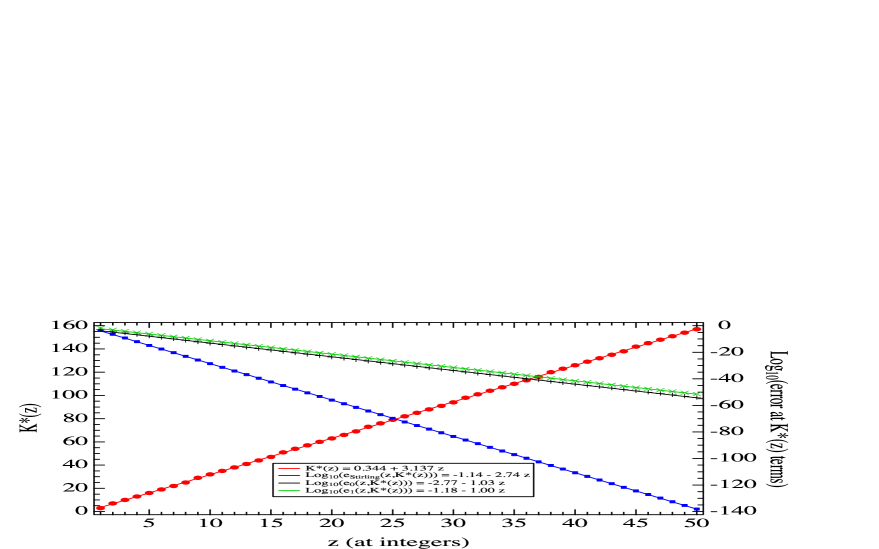
Figure 1: Optimal accuracy of Stirling’s asymptotic expansion: the optimal number of terms $K^{\ast}\left(z\right)$ (left axis) to achieve the lowest error $e_{\text{Stirling}}\left(z,K^{\ast}\left(z\right)\right)$ (right axis). The error $e_{0}\left(z,K^{\ast}\left(z\right)\right)$ and $e_{1}\left(z,K^{\ast}\left(z\right)\right)$ of Binet’s two factorial expansions for $\alpha=0$ and $\alpha=1$ are added (right axis). The legend shows linear fits of the data.

Fig. 1 shows the logarithm (in basis 10) of the error (right axis), evaluated at the optimal number of terms $K^{\ast}\left(z\right)$ versus $z$ (left axis). The comparison of Stirling’s asymptotic series with Binet’s two factorial expansions (6) for $\alpha=1$ and (38) for $\alpha=0$ clearly illustrates the amazing superiority of Stirling’s asymptotic series.

Fig. 2 illustrates that the logarithm of the error $e_{\alpha}\left(z,K^{\ast}\left(z\right)\right)$ versus $\alpha\in\left[-2,2\right]$ varies considerably. In particular around the zeros $\xi_{1}\left(m\right)$, $\xi_{2}\left(m\right)$ and $\xi_{3}\left(m\right)$ of the polynomial $b_{m}\left(\alpha\right)$ in the interval $\left[-2,2\right]$, the error of the generalized Binet factorial expansion (79) decreases sharply. The minimal errors, peaked around the zeros, only shift little in $\alpha$ for various $K^{\ast}\left(z\right)$ and $z$.

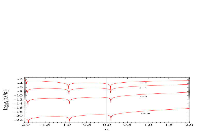
Figure 2: The logarithm of the error $e_{\alpha}\left(z,K^{\ast}\left(z\right)\right)$ versus $\alpha$ for various $z=\left\{2,4,8,16\right\}$.

Numerically for $m>10$, we found that the largest and only positive zero $\xi_{1}\left(m\right)\in\left[0.08,0.1\right]$ and that $\xi_{1}\left(m\right)$ attains its largest value 0.0963016 at $m=72$ and $\xi_{1}\left(m\right)$ slowly decreases for $m>72$. For any finite $K$, there exists a value of $\alpha$ around $\xi_{1}\left(K\right)$ that minimizes the error

$$e_{\alpha}\left(z,K\right) =\left|\mu\left(z\right)-\sum_{j=0}^{K}\left(\sum_{m=j+1}^{K}\frac{p_{j}\left(m\right)}{\prod_{k=0}^{m-1}(z+\alpha+k)}\right)\alpha^{j}\right|$$

$$=\left|\mu\left(z\right)-\frac{1}{12\left(z+\alpha\right)}\sum_{m=1}^{K}\prod_{j=1}^{m-1}\frac{\alpha-\xi_{j}\left(m\right)}{z+\alpha+j}\right|$$

Given $z$, the last form is related to a Padé approximant of order $\left[m-1/m+1\right]$ in $\alpha$.

If $K=K^{\ast}\left(z\right)$, then we can find a value $\alpha^{\ast}$ that has a comparable error $\left|e_{\alpha}\left(K\right)\right|$ than Stirling’s asymptotic approximation. For $z=10$ and $\alpha\in\left\{\frac{94909394316015843}{10^{18}},\frac{94909394316015845}{10^{18}}\right\}$, the error $\log_{10}\left|e_{\alpha}\left(10,K^{\ast}\left(10\right)\right)\right|<-30$, while Stirling’s lowest error is $\log_{10}\left|e_{\text{Stirling}}\left(10,K^{\ast}\left(10\right)\right)\right|=-28.5834$. The myth that Stirling’s approximation is always better than any factorial, convergent expansion for $\mu\left(z\right)$ with a same number of terms evaluated is not true, as illustrated by this counter example. If $\alpha^{\ast}$ is approximated by a rational number, then all coefficients of $b_{m}\left(\alpha\right)$ are rational numbers, just as the Bernoulli numbers in the Stirling approximation.

The major advantage of Binet’s series (79) over Stirling’s asymptotic (28) lies in its convergence, for all $\operatorname{Re}\left(z\right)>0$ and $\operatorname{Re}\left(\alpha\right)>-\operatorname{Re}\left(z\right)$, towards $\mu\left(z\right)$, which allows incorporation into integrals and series and may lead to other sharp bounds and approximations. Moreover, the “free” parameter $\alpha$ can be tuned to achieve a similar accuracy as the best accuracy of Stirling’s asymptotic series (78). Finally, the coefficients $\left|b_{m}\left(\alpha\right)\right|$ are monotonously increasing in $m>2$ and, for $\alpha>\xi_{1}\left(m\right)$, $b_{m}\left(\alpha\right)$ is positive, but only changes the sign once for $\xi_{2}\left(m\right)<\alpha<\xi_{1}\left(m\right)$. For finite $K$, it might be interesting to know the smallest possible error $e_{\alpha}\left(z,K\right)$ after optimization of $\alpha$.

8 Factorial series for Laplace transforms

The Laplace transform of a real function $f\left(t\right)$ is defined (see e.g. [25], [7, Chapter VII], [33]) for complex $z$ as

$$\varphi(z)=\mathcal{L}\left[f(t)\right]=\int_{0}^{\infty}e^{-zt}f(t)dt$$ (81)

with the inverse transform,

$$f(t)=\mathcal{L}^{-1}\left[\varphi(z)\right]=\frac{1}{2\pi i}\int_{c-i\infty}^{c+i\infty}\varphi(z)e^{zt}dz$$ (82)

where $c$ is the smallest real value of $\operatorname{Re}(z)$ for which the integral in (81) converges. Many functions can be defined by an integral as (81) as well as the probability generating function [30, Sec. 2.3.3] of a continuous random variable. For example, Binet’s integral (3) is a Laplace transform (81), where $\varphi(z)=\mu\left(z\right)$ and the integrand $f\left(t\right)=\frac{1}{t}\left(\frac{1}{e^{t}-1}-\frac{1}{t}+\frac{1}{2}\right)$ with $f\left(0\right)=\frac{1}{12}$.

Factorial series are hardly studied. By starting from Gudermann’s series (18), Jensen [15, art. 14] has demonstrated, without using integrals, that Binet’s factorial expansions are absolutely and uniformly convergent in some region of $z$. Temme has written a literature overview [24], of which parts were incorporated by Lauwerier in his book [16, p. 33-45], that devotes one chapter to factorial series. Parts of the content of [24] and [16, p. 33-45] are here absorbed. Apart from reviewing the literature more extensively than here, Delabaere and Rasoamanana [5] have presented similar results, but their method and exposition is rather different. In this Section 8, we generalize the idea of Binet’s proof of Theorem 1 as far as possible.

8.1 The analogon of Stirling’s asymptotic series

If we assume that the Taylor series $f\left(t\right)=\sum_{k=0}^{\infty}f_{k}t^{k}$, with Taylor coefficients $f_{k}=\frac{1}{k!}\left.\frac{d^{k}f(t)}{dt^{k}}\right|_{t=0}$, has an infinite radius of convergence, then the Laplace transform (81) can be expanded as

$$\varphi(z)=\int_{0}^{\infty}e^{-zt}f(t)dt=\sum_{k=0}^{\infty}f_{k}\int_{0}^{\infty}e^{-zt}t^{k}dt$$

into a Laurent series [26, Sec. 2.7]

$$\varphi(z)=\sum_{k=0}^{\infty}\frac{k!f_{k}}{z^{k+1}}$$ (83)

An infinite radius of convergence implies that the Taylor coefficient $f_{k}$ converges faster to zero than any exponential function, i.e. $f_{k}=o\left(e^{-ak}\right)$ for any finite $a$ and $k\rightarrow\infty$, and that $f\left(t\right)$ is an entire function. Most functions, however, are not entire functions. If the requirement of an infinite radius of convergence is ignored, then (83) may represent an asymptotic series $\varphi(z)=\sum_{k=0}^{K}\frac{k!f_{k}}{z^{k}}$, which diverges when $K\rightarrow\infty$. Indeed, repeated partial integration of the Laplace transform (81) yields

$$\varphi(z)=\sum_{k=0}^{K}\frac{k!f_{k}}{z^{k}}+\frac{1}{z^{K+1}}\int_{0}^{\infty}e^{-zt}f^{\left(K+1\right)}(t)dt$$ (84)

illustrating, for any $\operatorname{Re}\left(z\right)>c$ but $z\neq 0$ and real $t\geq 0$, that $\lim_{K\rightarrow\infty}\frac{f^{\left(K+1\right)}(t)}{z^{K+1}}$ must vanish to obtain a convergent Laurent series (83).

8.2 Binet’s method as a recipe in five steps

We formalize Binet’s proof of Theorem 1.

1. Binet’s substitution $e^{-t}=1-u$ or $t=-\log\left(1-u\right)$ in the integral (81) yields

   $$\varphi(z)=\int_{0}^{1}\left(1-u\right)^{z-1}f(-\log\left(1-u\right))du$$ (85)

   which converges for $\operatorname{Re}\left(z\right)>c$. Binet’s substitution is rather unusual, certainly in the study of Laplace integrals. In the early days, Euler represented the Gamma function in the form of (85), after letting $w=1-u$, as $\Gamma\left(z\right)=\int_{0}^{1}\log^{z-1}\left(\frac{1}{w}\right)dw$ (see e.g. [2, art. [1]]). Lauwerier [16, p. 33-35] and Temme [24] explain the success of the substitution $u=1-e^{-t}$ by comparing $u=re^{i\theta}$ confined to the unit disk $\left|u-1\right|<1$ at $u_{0}=1$ and the map $t=-\log\left(1-re^{i\theta}\right)$. In particular, the circle $\left|u-1\right|=1$ at $u_{0}=1$ with radius 1 maps into the curve

   $$t =-\log\left(1-\cos\theta-i\sin\theta\right)=-\log\left(\sqrt{2\left(1-\cos\theta\right)}e^{-i\arccos\frac{1-\cos\theta}{\sqrt{2\left(1-\cos\theta\right)}}}\right)$$

   $$=-\log\left(2\sin\frac{\theta}{2}\right)+i\arccos\left(\sin\frac{\theta}{2}\right)=-\log\left(2\sin\frac{\theta}{2}\right)+i\left(\frac{\pi-\theta}{2}\right)$$

   Hence, $\operatorname{Re}t=-\log\left(2\sin\frac{\theta}{2}\right)$ and $\operatorname{Im}t=\frac{\pi-\theta}{2}$ with $\theta\in\left[0,2\pi\right]$. Elimination of $\theta=\pi-2\operatorname{Im}t$ yields

   $$\operatorname{Re}t=-\log\left(2\cos\left(\operatorname{Im}t\right)\right)\hskip 28.45274pt\text{for }-\frac{\pi}{2}\leq\operatorname{Im}t\leq\frac{\pi}{2}$$ (86)

   The curve (86) is symmetric around the $\operatorname{Re}t$-axis due to $\cos\left(\operatorname{Im}t\right)=\cos\left(-\operatorname{Im}t\right)$ and $\cos\left(\operatorname{Im}t\right)\geq 0$ confines the curve (86) to the strip $-\frac{\pi}{2}\leq\operatorname{Im}t\leq\frac{\pi}{2}$, where the minimum occurs at $-\log 2$ for $\operatorname{Im}t=0$ and $\operatorname{Re}t$ grows boundlessly if $\operatorname{Im}t\rightarrow\pm\frac{\pi}{2}$. Thus, the map $t=-\log\left(1-u\right)$ of the unit disk $\left|u-1\right|<1$ appears as the interior $t$-region bounded by the curve (86). That $t$-region is considerably broader than the unit disk, which accounts for better results in the sense that the resulting factorial series in (88) below converges for more functions than its corresponding Laurent series (83).

2. The second step involves the Taylor expansion of $f(-\log\left(1-u\right))$ around $u_{0}=0$, where $\log\left(1-u_{0}\right)=0$. After Binet’s substitution $e^{-t}=1-u$, the Taylor series $f\left(t\right)=\sum_{k=0}^{\infty}f_{k}t^{k}$ becomes $f\left(-\log\left(1-u\right)\right)=\sum_{k=0}^{\infty}f_{k}\left(-\log\left(1-u\right)\right)^{k}$. Introducing the second generating function (43) of the Stirling numbers and reversing the $m$- and $k$-sum leads to

   $$f(-\log\left(1-u\right))=\sum_{m=0}^{\infty}\left(\sum_{k=0}^{m}\left.\frac{d^{k}f(t)}{dt^{k}}\right|_{t=0}\left(-1\right)^{m-k}S_{m}^{(k)}\,\right)\frac{u^{m}}{m!}$$ (87)

   Clearly, the Stirling numbers, which are integers, play a key role in Binet’s transformation $u=1-e^{-t}$.

3. Crucially for the third step, we assume that the Taylor series (87) converges for $\left|u\right|<1$. Hence, the radius of convergence of the Taylor series (87) should be at least equal to one. After substitution of the Taylor series (87) in the integral (85) and reversing the summation and integration operator, justified because a Taylor series can be term-wise integrated within its radius of convergence, yields

   $$\varphi(z)=\sum_{m=0}^{\infty}\left(\sum_{k=0}^{m}\left.\frac{d^{k}f(t)}{dt^{k}}\right|_{t=0}\left(-1\right)^{m-k}S_{m}^{(k)}\,\right)\frac{1}{m!}\int_{0}^{1}u^{m}\left(1-u\right)^{z-1}du$$

4. The fourth step uses the Beta integral $\int_{0}^{1}u^{p-1}\left(1-u\right)^{q-1}du=\frac{\Gamma\left(p\right)\Gamma\left(q\right)}{\Gamma\left(p+q\right)}$, valid for $\operatorname{Re}\left(p\right)>0$ and $\operatorname{Re}\left(q\right)>0$, and leads to

   $$\varphi(z)=\sum_{m=0}^{\infty}\left(\sum_{k=0}^{m}\left.\frac{d^{k}f(t)}{dt^{k}}\right|_{t=0}\left(-1\right)^{m-k}S_{m}^{(k)}\,\right)\frac{\Gamma\left(z\right)}{\Gamma\left(m+1+z\right)}$$

5. The fifth and final step replaces $\frac{\Gamma\left(z+m\right)}{\Gamma\left(z\right)}=\prod_{k=0}^{m-1}(z+k)$ and we arrive at the factorial expansion, valid for $\operatorname{Re}\left(z\right)>c$,

   $$\varphi(z)=\sum_{m=0}^{\infty}\frac{\sum_{k=0}^{m}\left.\frac{d^{k}f(t)}{dt^{k}}\right|_{t=0}\left(-1\right)^{m-k}S_{m}^{(k)}}{\prod_{k=0}^{m}(z+k)}$$ (88)

The factorial expansion (88) generalizes Binet’s second factorial expansion (38) in Theorem 1.

8.3 Infinitely many factorial series for $\varphi(z)$

We generalize the recipe with five steps in Section 8.2, as we did for the particular case $\varphi(z)=\mu\left(z\right)$ in Theorem 3, together with an additional $\beta$-scaling inspired by Temme [24, p. 11]. Our main result is:

Theorem 4

Only if the Taylor series

$$f(-\beta\log\left(1-u\right))=\sum_{m=0}^{\infty}\left(\sum_{k=0}^{m}k!f_{k}\beta^{k}\left(-1\right)^{m-k}S_{m}^{(k)}\,\right)\frac{u^{m}}{m!}$$ (89)

has a radius of convergence at least equal to 1, then the Laplace transform $\varphi(z)$ of the function $f\left(t\right)$ possesses infinitely many factorial series in the complex parameter $\alpha$ and real $\beta>0$, for $\operatorname{Re}\left(z\right)>c$ and $\frac{\operatorname{Re}\left(\alpha\right)}{\beta}>-\operatorname{Re}\left(z\right)$,

$$\varphi(z)=\beta\sum_{m=0}^{\infty}\frac{m!\phi_{m}\left(\alpha,\beta\right)}{\prod_{k=0}^{m}(\beta z+\alpha+k)}$$ (90)

where

$$\phi_{m}\left(\alpha,\beta\right)=\frac{1}{m!}\sum_{k=0}^{m}\left(\sum_{j=0}^{m-k}\left(k+j\right)!S_{m}^{(k+j)}\left(-1\right)^{m-\left(k+j\right)}f_{j}\beta^{j}\right)\frac{\alpha^{k}}{k!}$$ (91)

Further, $\phi_{m}\left(\alpha,\beta\right)$ is a polynomial of degree $m$ in $\alpha$ with highest order term $\frac{f(0)}{m!}\alpha^{m}$ and $\phi_{0}\left(\alpha,\beta\right)=f(0)$. A complex integral for $\phi_{m}\left(\alpha,\beta\right)$, where the contour $C\left(0\right)$ encloses the point $\omega_{0}=0$, is

$$\phi_{m}\left(\alpha,\beta\right)=\frac{\left(-1\right)^{m}}{2\pi i}\int_{C(0)}\frac{f(-\beta\log\left(1+\omega\right))d\omega}{\left(1+\omega\right)^{\alpha}\omega^{m+1}}$$ (92)

while another compact form is

$$\phi_{m}\left(\alpha,\beta\right)=\frac{1}{m!}\sum_{j=0}^{m}\left.\frac{d^{j}}{dt^{j}}\left(f(t)e^{\frac{\alpha}{\beta}t}\right)\right|_{t=0}S_{m}^{(j)}\left(-1\right)^{m-j}\beta^{j}$$ (93)

Clearly, the factorial series in (90) with (93) reduces to (88) for $\alpha=0$ and $\beta=1$.

Proof: We repeat the five steps in Section 8.2, but we rewrite the Laplace transform (85) of $\varphi(z)$ after a generalization of Binet’s substitution $e^{-t}=\left(1-u\right)^{\beta}$ or $t=-\beta\log\left(1-u\right)$ as

$$\varphi(z)=\beta\int_{0}^{1}\left(1-u\right)^{\beta z+\alpha-1}\left(1-u\right)^{-\alpha}f(-\beta\log\left(1-u\right))du$$

which still converges for $\operatorname{Re}\left(z\right)>c$, in spite of the introduction of the “free” parameter $\alpha$ and the real $\beta>0$.

The second step now involves the Taylor expansion of

$$g\left(u;\alpha,\beta\right)=\left(1-u\right)^{-\alpha}f(-\beta\log\left(1-u\right))=\sum_{m=0}^{\infty}\phi_{m}\left(\alpha,\beta\right)u^{m}$$ (94)

around $u_{0}=0$. The Taylor series $f(-\beta\log\left(1-u\right))$ in (89) follows from (87). The Taylor series $\left(1-u\right)^{-\alpha}=\sum_{k=0}^{\infty}\binom{-\alpha}{k}\left(-1\right)^{k}u^{k}$ is valid for any complex $\alpha$ provided $\left|u\right|<1$. Thus, the radius of convergence of (94) is limited to 1 by $\left(1-u\right)^{-\alpha}$, which is just sufficient for the reversal of summation and integration in step three, provided the radius of convergence of $g\left(u;0,\beta\right)=f(-\beta\log\left(1-u\right))$ in (87) is at least equal to 1. From Cauchy’s integral theorem [26] we directly find the integral representation (92). In addition, the Taylor coefficient $\phi_{m}\left(\alpha,\beta\right)$ in (94) follows from the Cauchy product

$$\phi_{m}\left(\alpha,\beta\right)=\sum_{j=0}^{m}\binom{-\alpha}{m-j}\frac{\left(-1\right)^{m-j}}{j!}\sum_{l=0}^{j}l!f_{l}\beta^{l}\left(-1\right)^{j-l}S_{j}^{(l)}$$ (95)

The remaining steps in Binet’s method of Section 8.2, consisting of the substitution of the Taylor series (94) of $g\left(u;\alpha,\beta\right)$ in the integral, the reversal of integral and summation and the explicit evaluation of the remaining Beta integral,

$$\varphi(z)=\beta\sum_{m=0}^{\infty}\phi_{m}\left(\alpha,\beta\right)\int_{0}^{1}\left(1-u\right)^{\beta z+\alpha-1}u^{m}du=\beta\sum_{m=0}^{\infty}\phi_{m}\left(\alpha,\beta\right)\frac{m!\Gamma\left(\beta z+\alpha\right)}{\Gamma\left(\beta z+\alpha+m+1\right)}$$

lead to the factorial expansion (90), valid for $\operatorname{Re}\left(z\right)>c$ and $\frac{\operatorname{Re}\left(\alpha\right)}{\beta}>-\operatorname{Re}\left(z\right)$.

The remainder of the proof consists of simplifying the Taylor coefficient $\phi_{m}\left(\alpha,\beta\right)$ in (95). It is convenient to reverse the summations,

$$\phi_{m}\left(\alpha,\beta\right)=\sum_{l=0}^{m}l!f_{l}\beta^{l}\sum_{j=l}^{m}\frac{\Gamma\left(1-\alpha\right)}{\Gamma\left(1-\alpha-m+j\right)}\frac{\left(-1\right)^{m-l}}{\left(m-j\right)!j!}S_{j}^{(l)}$$

We introduce the generating function (42) of the Stirling numbers $S_{m}^{(k)}$,

$$\phi_{m}\left(\alpha,\beta\right)=\frac{1}{m!}\sum_{l=0}^{m}l!f_{l}\beta^{l}\sum_{j=l}^{m}\binom{m}{j}\left(-1\right)^{m-l}S_{j}^{(l)}\sum_{k=0}^{m-j}S_{m-j}^{(k)}\left(-1\right)^{k}\;\alpha^{k}$$

Let $q=m-j$ in the double sum

$$T=\sum_{j=l}^{m}\binom{m}{j}\left(-1\right)^{m-l}S_{j}^{(l)}\sum_{k=0}^{m-j}S_{m-j}^{(k)}\;\left(-1\right)^{k}\alpha^{k}=\left(-1\right)^{m-l}\sum_{q=0}^{m-l}\binom{m}{q}S_{m-q}^{(l)}\sum_{k=0}^{q}S_{q}^{(k)}\;\left(-1\right)^{k}\alpha^{k}$$

and after reversing the sums, we obtain $T=\left(-1\right)^{m-l}\sum_{k=0}^{m-l}\left(\sum_{q=k}^{m-l}\binom{m}{q}S_{q}^{(k)}S_{m-q}^{(l)}\right)\left(-1\right)^{k}\alpha^{k}$. Using (68) and $S_{q}^{(m)}=0$ if $m>q$ gives $\sum_{q=k}^{m-l}\binom{m}{q}S_{q}^{(k)}S_{m-q}^{(l)}=\sum_{q=0}^{m}\binom{m}{q}S_{q}^{(k)}S_{m-q}^{(l)}=\frac{\left(k+l\right)!}{l!k!}S_{m}^{(k+l)}$, resulting in

$$T=\frac{\left(-1\right)^{m-l}}{l!}\sum_{k=0}^{m-l}\frac{\left(k+l\right)!}{k!}S_{m}^{(k+l)}\left(-1\right)^{k}\alpha^{k}$$

Hence, the Taylor coefficient (95) becomes

$$\phi_{m}\left(\alpha,\beta\right)=\frac{1}{m!}\sum_{l=0}^{m}f_{l}\beta^{l}\sum_{k=0}^{m-l}\frac{\left(k+l\right)!}{k!}S_{m}^{(k+l)}\left(-1\right)^{m-\left(l+k\right)}\alpha^{k}$$ (96)

which we can express as a polynomial in $\alpha$ by letting $n=m-l$

$$\phi_{m}\left(\alpha,\beta\right)=\frac{1}{m!}\sum_{n=0}^{m}f_{m-n}\beta^{m-n}\sum_{k=0}^{n}\frac{\left(k+m-n\right)!}{k!}S_{m}^{(k+m-n)}\left(-1\right)^{n+k}\alpha^{k}$$

After reversing the sums and letting $j=m-n$, we arrive at (91). Reversing the sums in (91)

$$\phi_{m}\left(\alpha,\beta\right)=\frac{1}{m!}\sum_{j=0}^{m}\left(\sum_{k=0}^{j}\binom{j}{k}\left.\frac{d^{j-k}f(t)}{dt^{j-k}}\right|_{t=0}\left(\frac{\alpha}{\beta}\right)^{k}\right)S_{m}^{(j)}\left(-1\right)^{m-j}\beta^{j}$$

substituting $\left(\frac{\alpha}{\beta}\right)^{k}=\left.\frac{d^{k}}{dt^{k}}e^{\frac{\alpha}{\beta}t}\right|_{t=0}$ into the $k$-sum in brackets

$$\sum_{k=0}^{j}\binom{j}{k}\left.\frac{d^{j-k}f(t)}{dt^{j-k}}\right|_{t=0}\left(\frac{\alpha}{\beta}\right)^{k}=\sum_{k=0}^{j}\binom{j}{k}\left.\frac{d^{j-k}f(t)}{dt^{j-k}}\right|_{t=0}\left.\frac{d^{k}}{dt^{k}}e^{\frac{\alpha}{\beta}t}\right|_{t=0}=\left.\frac{d^{j}}{dt^{j}}\left(f(t)e^{\frac{\alpha}{\beta}t}\right)\right|_{t=0}$$

where Leibniz’s rule has been used, demonstrates (93) and proves Theorem 4. $\square\vskip 6.0pt plus 2.0pt minus 2.0pt$

A verification of Theorem 4 by computing the inverse Laplace transform is given in Appendix F. Lauwerier [16, p. 35] interestingly mentions that, due to the asymptotic relation $\frac{\Gamma\left(m\right)}{\Gamma\left(z+m\right)}\sim m^{-z}$ for large $m$, the factorial series (90) for $\beta=1$, rewritten as

$$\varphi(z)=\Gamma\left(z+\alpha\right)\sum_{m=1}^{\infty}\frac{\Gamma\left(m\right)}{\Gamma\left(z+\alpha+m\right)}\phi_{m-1}\left(\alpha,1\right)$$

and the corresponding Dirichlet series $\varphi_{D}(z)=\sum_{m=1}^{\infty}\frac{m^{\alpha}\phi_{m-1}\left(\alpha,1\right)}{m^{-z}}$ have the same converge range for $\operatorname{Re}\left(z\right)>c$. Consequently, the rich theory of Dirichlet series (see e.g. [26, 27]) directly applies to convergence aspect of the factorial series (90). Reviewing Landau’s work on the factorial series, Temme [24] adds Newton’s series $\sum_{m=0}^{\infty}\left(-1\right)^{m}\binom{z-1}{m}\phi_{m-1}\left(\alpha,1\right)$ to the factorial and Dirichlet series as the third type of series with the same convergence range.

Lauwerier [16, p. 42-43] gives examples of factorial series (90) with $\alpha=0$ and $\beta=1$. Temme [24] provides even more interesting examples such as $\varphi(z)=\int_{0}^{\infty}\frac{e^{-zt}dt}{\left(1+t\right)^{\nu}}$. Here, we add:

Example 1 If $f\left(t\right)=e^{bt}$, then $\mathcal{L}\left[e^{bt}\right]=\frac{1}{z-b}$ and the corresponding factorial polynomial $\phi_{m}\left(\alpha,1\right)$ in (93) is, with $\left.\frac{d^{k}}{dt^{k}}\left(f(t)e^{\alpha t}\right)\right|_{t=0}=\left.\frac{d^{k}}{dt^{k}}\left(e^{\left(\alpha+b\right)t}\right)\right|_{t=0}=\left(\alpha+b\right)^{k}$ and the generating function (42),

$$m!\left.\phi_{m}\left(\alpha,1\right)\right|_{e^{bt}}=\sum_{k=0}^{m}\left(\alpha+b\right)^{k}\left(-1\right)^{m-k}S_{m}^{(k)}=\prod_{k=0}^{m-1}(\alpha+b+k)$$

The factorial series (90) becomes, for $\operatorname{Re}\left(z\right)>b$,

$$\frac{1}{z-b}=\sum_{m=0}^{\infty}\frac{\prod_{k=0}^{m-1}(b+\alpha+k)}{\prod_{k=0}^{m}(z+\alpha+k)}=\frac{\Gamma\left(z+\alpha\right)}{\Gamma\left(b+\alpha\right)}\sum_{m=0}^{\infty}\frac{\Gamma\left(b+\alpha+m\right)}{\Gamma\left(z+\alpha+m+1\right)}$$ (97)

which is known for $\alpha=0$ (see e.g. Nielsen [18, band I, p. 77]). Indeed, Gauss’s classical result [1, 15.1.20] for the hypergeometric series at $z=1$ is, for $c\neq-k$ ($k$ integer) and Re$\left(c-a-b\right)>0$,

$$F\left(a,b;c;1\right)=\frac{\Gamma(c)\Gamma(c-a-b)}{\Gamma(c-a)\Gamma(c-b)}=\frac{\Gamma(c)}{\Gamma(a)\Gamma(b)}\sum_{m=0}^{\infty}\frac{\Gamma(a+m)\Gamma(b+m)}{\Gamma(c+m)m!}$$ (98)

For $a=1$, $b\rightarrow b+\alpha$ and $c=z+\alpha+1$, Gauss’s formula (98) reduces to (97).

Example 2 Let $f\left(t\right)=E_{a,b}\left(t\right)=\sum_{k=0}^{\infty}\frac{t^{k}}{\Gamma\left(b+ak\right)}$, which is the Mittag-Leffler function [10]. The Laplace transform (see e.g. [31, art. 20]) is

$$\int_{0}^{\infty}e^{-zt}t^{\gamma-1}E_{a,b}\left(xt^{\beta}\right)dt=\sum_{k=0}^{\infty}\frac{\Gamma\left(\gamma+\beta k\right)}{\Gamma\left(b+ak\right)}\frac{x^{k}}{z^{\gamma+k\beta}}$$ (99)

valid for $\left|\beta\right|\leq\left|a\right|$ and $\gamma>0$. For $\gamma=\beta=x=1$, the Laplace transform (99) simplifies to a Laurent series (83) in $z$. The corresponding factorial polynomial (91) can be written as

$$m!\left.\phi_{m}\left(\alpha,\beta\right)\right|_{E_{a,b}\left(t\right)}=\sum_{j=0}^{m}\left(\sum_{k=0}^{j}\frac{j!}{\Gamma\left(b+a\left(j-k\right)\right)k!}\left(\frac{\alpha}{\beta}\right)^{k}\right)S_{m}^{(j)}\left(-1\right)^{m-j}\beta^{j}$$

where the $k$-sum reduces to $\left(1+\frac{\alpha}{\beta}\right)^{j}$ for $a=b=1$, in which case $E_{1,1}\left(t\right)=e^{t}$ simplifying to example 1. Unfortunately, for arbitrary $a$ and $b$, we could not simply $\left.\phi_{m}\left(\alpha,\beta\right)\right|_{E_{a,b}\left(t\right)}$ for the Mittag-Leffler function $E_{a,b}\left(t\right)$.

On the other hand, after replacing $z\rightarrow kz$ in factorial series (90), multiplying both sides by $x^{k}$ and adding over all $k\geq 0$, we formally obtain a Mittag-Leffler transformation

$$\sum_{k=0}^{\infty}\frac{x^{k}\varphi(zk)}{\Gamma\left(\beta zk+\alpha\right)}=\int_{0}^{\infty}f(t)E_{\beta z,\alpha}\left(xe^{-zt}\right)dt=\beta\sum_{m=0}^{\infty}\phi_{m}\left(\alpha,\beta\right)m!E_{\beta z,\alpha+m+1}\left(x\right)$$

8.4 Open question

The factorial series (90) of a non-entire function may converge, whereas the Laurent series (83) does not. An example is the Binet function $\mu\left(z\right)$, whose Laurent series (83) is Stirling’s famous asymptotic, but divergent series (28). Hence, the question arises: “Given the Taylor series $f\left(t\right)=\sum_{k=0}^{\infty}f_{k}t^{k}$ with radius of convergence $R_{f}$, when does a factorial series (90) of the Laplace transform $\varphi(z)$ converge?”

We can only give a partial insight. The recipe in 5 steps for a factorial series (90) of the Laplace transform $\varphi(z)$ requires that the Taylor series (89) of $g\left(u;0,\beta\right)=f(-\beta\log\left(1-u\right))$ around the origin $u_{0}=0$ converges within the unit circle. Its corresponding Taylor coefficient is written in terms of $f_{k}=\frac{1}{k!}\left.\frac{d^{k}f(t)}{dt^{k}}\right|_{t=0}$ as $g_{0}=f_{0}$ and

$$g_{m}\left(\beta\right)=\frac{1}{m!}\sum_{k=1}^{m}k!f_{k}\beta^{k}\left(-1\right)^{m-k}S_{m}^{(k)}\,\hskip 28.45274pt\text{for }m>0$$ (100)

from which it follows that, for $m>0$, the Taylor coefficient $g_{m}\left(\beta\right)$ is independent of $f_{0}=f\left(0\right)$ (like any characteristic coefficient (115)). The inverse transform of (100)

$$\beta^{m}f_{m}=\frac{1}{m!}\sum_{k=1}^{m}k!g_{k}\left(\beta\right)\left(-1\right)^{m-k}\mathcal{S}_{m}^{(k)}\hskip 28.45274pt\text{for }m>0$$ (101)

where $\mathcal{S}_{m}^{(k)}$ is the Stirling number of the Second Kind, is deduced as in the proof of Property 5.

In contrast to $S_{m}^{(k)}$, the Stirling numbers $\mathcal{S}_{m}^{(k)}$ are non-negative. Thus, $\left(-1\right)^{m-k}S_{m}^{(k)}>0$ in (100), whereas $\left(-1\right)^{k}\mathcal{S}_{m}^{(k)}$ in (101) is alternating with $k$. If $f_{k}$ is non-negative, then (100) indicates that also $g_{m}\left(\beta\right)$ is non-negative. Moreover, (100) written as $g_{m}\left(\beta\right)=f_{m}+\frac{1}{m!}\sum_{k=1}^{m-1}k!f_{k}\left(-1\right)^{m-k}S_{m}^{(k)}$ then shows that $g_{m}\left(\beta\right)\geq f_{m}$. Consequently, the radius $R_{g}$ of convergence of $g\left(u;0,\beta\right)=f(-\beta\log\left(1-u\right))=\sum_{m=0}^{\infty}g_{m}\left(\beta\right)u^{m}$ is not larger than the radius $R_{f}$ of convergence of $f\left(t\right)=\sum_{k=0}^{\infty}f_{k}t^{k}$. However, if $f_{k}$ is non-negative, then the non-entire function $f\left(t\right)$ has a pole at a finite, real $t=R_{f}$ and its Laplace integral $\varphi(z)$ in (81) does not exist. On the other hand, if $f_{k}=\left(-1\right)^{k}\left|f_{k}\right|$ is alternating, then $f\left(-t\right)$ has non-negative Taylor coefficients so that $f\left(t\right)$ is decreasing in $t$. The Laplace integral $\varphi(z)$ exists for decreasing functions $f\left(t\right)$. If $g_{m}\left(\beta\right)=\left(-1\right)^{m}\left|g_{m}\left(\beta\right)\right|$ is alternating, then (101) shows that $f_{m}=\left(-1\right)^{m}\left(\left|g_{m}\left(\beta\right)\right|+\frac{1}{m!}\sum_{k=1}^{m-1}k!\left|g_{k}\left(\beta\right)\right|\mathcal{S}_{m}^{(k)}\right)$ is alternating and $\left|f_{m}\right|>\left|g_{m}\left(\beta\right)\right|$, implying that the radius of convergence $R_{g}\geq R_{f}$.

In summary, if $f_{k}=\left(-1\right)^{k}\left|f_{k}\right|$ is alternating, then the factorial series (90) has higher probability of convergence than its corresponding Laurent series (83).

Acknowledgement I am very grateful to the late R. B. Paris and R. E. Kooij for pointing to a few misprints in an early version and to A. Olde Daalhuis for pointing me to Nemes’ paper [17]. After completing this paper, G. Nemes has informed me about the work of Shi et al. [23], whose Theorem 1 is essentially the same as our Theorem 3, though their coefficient for $b_{m}\left(\alpha\right)$ is only mentioned in integral form, different from (56), and our validity range of $\alpha$ is slightly broader. Moreover, our proof(s) and approach are entirely different. A. Olde Daalhuis and G. Nemes pointed me to the book of Lauwerier [16] and to [5]. N. Temme has sent me his earlier report [24] of which parts appeared in Lauwerier’s book.

Appendix A Complex integral for Binet’s function $\mu\left(z\right)$

A.1 Derivation of the complex integral in (24)

From Weierstrass’s product (30) of the Gamma function, Whittaker and Watson [32, p. 277] deduce the formula, valid for all $a$ and $z$,

$$\log\frac{\Gamma\left(a\right)}{\Gamma\left(z+a\right)}=-z\frac{\Gamma^{\prime}\left(a\right)}{\Gamma\left(a\right)}+\frac{1}{2\pi i}\int_{q-i\infty}^{q+i\infty}\frac{\pi}{\sin\pi s}\frac{\zeta\left(s,a\right)}{s}z^{s}ds\hskip 28.45274pt\text{with }1<q<2$$

where $\zeta\left(s,a\right)=\sum_{n=0}^{\infty}\frac{1}{\left(n+a\right)^{s}}$ is the Hurwitz Zeta-function, which reduces for $a=1$ to the Riemann Zeta-function $\zeta\left(s\right)$. Thus, for $a=1$ and $\frac{\Gamma^{\prime}\left(1\right)}{\Gamma\left(1\right)}=-\gamma$, where $\gamma$ is the Euler constant, we have

$$\log\Gamma\left(z+1\right)=-\gamma z-\frac{1}{2\pi i}\int_{q-i\infty}^{q+i\infty}\frac{\pi}{\sin\pi s}\frac{\zeta\left(s\right)}{s}z^{s}ds\hskip 28.45274pt\text{with }1<q<2$$

If we move the line of integration to $0<c=\operatorname{Re}\left(s\right)<1$, we encounter a double pole at $s=1$, because $\zeta\left(s\right)=\frac{1}{s-1}+\gamma+O\left(s-1\right)$ around $s=1$ and a zero of $\sin\pi s$. The residue at $s=1$ follows from Cauchy’s integral theorem $\frac{1}{k!}\;\left.\frac{d^{k}f(z)}{dz^{k}}\right|_{z=z_{0}}=\frac{1}{2\pi i}\int_{C(z_{0})}\frac{f(\omega)\;d\omega}{(\omega-z_{0})^{k+1}}$, where $f\left(z\right)$ is analytic within the contour $C\left(z_{0}\right)$ that encloses the point $z_{0}$ and we obtain

$$\frac{1}{2\pi i}\int_{q-i\infty}^{q+i\infty}\frac{\pi}{\sin\pi s}\frac{\zeta\left(s\right)}{s}z^{s}ds=\frac{1}{2\pi i}\int_{c-i\infty}^{c+i\infty}\frac{\pi}{\sin\pi s}\frac{\zeta\left(s\right)}{s}z^{s}ds+\lim_{s\rightarrow 1}\frac{d}{ds}\left(\frac{z^{s}}{s}\frac{\pi\zeta\left(s\right)\left(s-1\right)^{2}}{\sin\pi s}\right)$$

because the function between brackets is analytic at $s=1$. Executing the derivative,

$$\frac{d}{ds}\left(\frac{z^{s}}{s}\frac{\pi\zeta\left(s\right)\left(s-1\right)^{2}}{\sin\pi s}\right)=\frac{z^{s}\pi\left(s-1\right)}{s\sin\pi s}\left(\left(\log z-\frac{1}{s}\right)\zeta\left(s\right)\left(s-1\right)+\zeta^{\prime}\left(s\right)\left(s-1\right)+2\zeta\left(s\right)-\frac{\pi\zeta\left(s\right)\left(s-1\right)\cos\pi s}{\sin\pi s}\right)$$

and using the Taylor expansions of $\left(s-1\right)\zeta\left(s\right)$ around $s=1$ gives us

$$\lim_{s\rightarrow 1}\frac{d}{ds}\left(\frac{z^{s}}{s}\frac{\pi\zeta\left(s\right)\left(s-1\right)^{2}}{\sin\pi s}\right)=-z\left(\log z-1+\gamma\right)$$

and we obtain, for $0<c<1$,

$$\log\Gamma\left(z+1\right)=z\log z-z-\frac{1}{2\pi i}\int_{c-i\infty}^{c+i\infty}\frac{\pi}{\sin\pi s}\frac{\zeta\left(s\right)}{s}z^{s}ds$$

Moving the line of integration over the double pole at $s=0$ to the left yields, for $-1<c^{\prime}<0$,

$$\log\Gamma\left(z+1\right)=z\log z-z-\frac{1}{2\pi i}\int_{c^{\prime}-i\infty}^{c^{\prime}+i\infty}\frac{\pi}{\sin\pi s}\frac{\zeta\left(s\right)}{s}z^{s}ds-\lim_{s\rightarrow 0}\frac{d}{ds}\left(\frac{\pi s\zeta\left(s\right)}{\sin\pi s}z^{s}\right)$$

The derivative is

$$\frac{d}{ds}\left(\frac{s\zeta\left(s\right)}{\sin\pi s}z^{s}\right)=\frac{z^{s}\zeta\left(s\right)s}{\sin\pi s}\left\{\frac{1}{s}-\frac{\pi\cos\pi s}{\sin\pi s}+\log z+\frac{\zeta^{\prime}\left(s\right)}{\zeta\left(s\right)}\right\}$$

Since $\pi\cot\left(\pi x\right)=\frac{1}{x}-2\sum_{n=1}^{\infty}\zeta\left(2n\right)\,x^{2n-1}$, we find that $\lim_{s\rightarrow 0}\frac{1}{s}-\pi\cot\left(\pi s\right)=0$ and

$$\lim_{s\rightarrow 0}\frac{ds}{ds}\left(\frac{\pi s\zeta\left(s\right)}{\sin\pi s}z^{s}\right)=\zeta\left(0\right)\left\{\log z+\frac{\zeta^{\prime}\left(0\right)}{\zeta\left(0\right)}\right\}$$

With $\zeta\left(0\right)=-\frac{1}{2}$ and $\zeta^{\prime}\left(0\right)=-\frac{1}{2}\log(2\pi)$, we arrive at $\lim_{s\rightarrow 0}\frac{ds}{ds}\left(\frac{\pi s\zeta\left(s\right)}{\sin\pi s}z^{s}\right)=-\frac{1}{2}\left\{\log z+\log(2\pi)\right\}$ and

$$\log\Gamma\left(z+1\right)=\left(z+\frac{1}{2}\right)\log z-z+\frac{1}{2}\log(2\pi)-\frac{1}{2\pi i}\int_{c^{\prime}-i\infty}^{c^{\prime}+i\infty}\frac{\pi}{\sin\pi s}\frac{\zeta\left(s\right)}{s}z^{s}ds\hskip 28.45274pt\text{with }-1<c^{\prime}<0$$

From the definition $\log\Gamma\left(z\right)=\left(z-\frac{1}{2}\right)\log z-z+\frac{1}{2}\log\left(2\pi\right)+\mu\left(z\right)$, we find (24).

We present a second, shorter derivation of (24) by employing the inverse Mellin transform

$$\frac{1}{e^{2\pi t}-1}=\frac{1}{2\pi i}\int_{c-i\infty}^{c+i\infty}\Gamma\left(s\right)\zeta\left(s\right)\left(2\pi t\right)^{-s}ds\hfill\hskip 28.45274pt\text{for }c>1$$

Substitution into Binet’s integral (2) and reversing the integrals gives

$$\mu\left(z\right)=2\int_{0}^{\infty}\frac{\arctan\left(\frac{t}{z}\right)}{e^{2\pi t}-1}dt=\frac{1}{\pi i}\int_{c-i\infty}^{c+i\infty}\Gamma\left(s\right)\zeta\left(s\right)\left(2\pi\right)^{-s}\left(\int_{0}^{\infty}\arctan\left(\frac{t}{z}\right)t^{-s}dt\right)ds$$

Partial integration, followed by a substitution $u=\left(\frac{t}{z}\right)^{2}$ and the use of the Beta integral and the Gamma reflection formula results in

$$-\int_{0}^{\infty}\arctan\left(\frac{t}{z}\right)t^{-s}dt=\frac{z^{1-s}\pi}{2\left(1-s\right)\sin\frac{\pi s}{2}}$$

and

$$\mu\left(z\right)=-\frac{z}{2i}\int_{c-i\infty}^{c+i\infty}\zeta\left(s\right)\frac{\Gamma\left(s\right)\left(2\pi z\right)^{-s}}{\left(1-s\right)\sin\frac{\pi s}{2}}ds$$

Using the functional equation $\zeta(s)=2(2\pi)^{s-1}\sin\frac{\pi s}{2}\Gamma(1-s)\zeta(1-s)$ yields

$$\mu\left(z\right)=-\frac{1}{2\pi i}\int_{c-i\infty}^{c+i\infty}\frac{\pi}{\sin\pi s}\frac{\zeta(1-s)}{\left(1-s\right)}z^{1-s}ds\hskip 28.45274pt\text{with }1<c<2$$

and a change of variable $w=1-s$ then returns again the complex integral in (24).

A.2 Derivation of the convergent series (31)

Substituting the Taylor series $\left(s-1\right)\zeta\left(s\right)=\sum_{m=0}^{\infty}g_{m}\left(1\right)\left(s-1\right)^{m}$ into the integral (24) yields

$$\mu\left(z\right) =-\frac{1}{2\pi i}\int_{c-i\infty}^{c+i\infty}\frac{\pi}{\sin\pi s}\frac{\zeta\left(s\right)}{s}z^{s}ds\hskip 28.45274pt\text{with }-1<c<0$$

$$=-\frac{1}{2\pi i}\int_{c-i\infty}^{c+i\infty}\frac{\pi}{\sin\pi s}\frac{1}{s\left(s-1\right)}\sum_{m=0}^{\infty}g_{m}\left(1\right)\left(s-1\right)^{m}z^{s}ds$$

Integration and summation can be reversed, because the Taylor series converges for all complex $s$ and within the radius of convergence, a Taylor series represents an analytic function that can be integrated and differentiated [26, p. 97],

$$\mu\left(z\right) =-\sum_{m=0}^{\infty}g_{m}\left(1\right)\frac{1}{2\pi i}\int_{c-i\infty}^{c+i\infty}\frac{\pi}{\sin\pi s}\frac{\left(s-1\right)^{m}z^{s}}{s\left(s-1\right)}ds$$

$$=-\frac{1}{2\pi i}\int_{c-i\infty}^{c+i\infty}\frac{\pi}{\sin\pi s}\frac{z^{s}}{s\left(s-1\right)}ds-\sum_{m=1}^{\infty}g_{m}\left(1\right)\frac{1}{2\pi i}\int_{c-i\infty}^{c+i\infty}\frac{\pi}{\sin\pi s}\frac{\left(s-1\right)^{m-1}z^{s}}{s}ds$$

We evaluate the first integral. If $\left|z\right|\leq 1$, then we close the contour over the positive $\operatorname{Re}\left(s\right)$-plane (where the integral over semi-circle at infinity vanishes). Cauchy’s residu theorem tells us that

$$-\frac{1}{2\pi i}\int_{c-i\infty}^{c+i\infty}\frac{\pi}{\sin\pi s}\frac{z^{s}}{s\left(s-1\right)}ds =\pi\sum_{n=2}^{\infty}\lim_{s\rightarrow n}\frac{\left(s-n\right)}{\sin\pi s}\frac{z^{s}}{s\left(s-1\right)}+\pi\lim_{s\rightarrow 0}\frac{d}{ds}\frac{s}{\sin\pi s}\frac{z^{s}}{\left(s-1\right)}$$

$$+\pi\lim_{s\rightarrow 1}\frac{d}{ds}\frac{\left(s-1\right)}{\sin\pi s}\frac{z^{s}}{s}$$

With

$$\frac{d}{ds}\frac{s}{\sin\pi s}\frac{z^{s}}{\left(s-1\right)}=\frac{s}{\sin\pi s}\frac{z^{s}}{\left(s-1\right)}\left\{\frac{1}{s}-\pi\cot\pi s+\log z-\frac{1}{\left(s-1\right)}\right\}$$

Since $\lim_{s\rightarrow 0}\frac{1}{s}-\pi\cot\pi s=0$, we find that

$$\pi\lim_{s\rightarrow 0}\frac{d}{ds}\frac{s}{\sin\pi s}\frac{z^{s}}{\left(s-1\right)}=-\left(\log z+1\right)\lim_{s\rightarrow 0}\frac{\pi s}{\sin\pi s}=-\left(\log z+1\right)$$

and, similarly, that

$$\pi\lim_{s\rightarrow 1}\frac{d}{ds}\frac{\left(s-1\right)}{\sin\pi s}\frac{z^{s}}{s}=-z\left(\log z-1\right)$$

Hence, for $\left|z\right|\leq 1$,

$$-\frac{1}{2\pi i}\int_{c-i\infty}^{c+i\infty}\frac{\pi}{\sin\pi s}\frac{z^{s}}{s\left(s-1\right)}ds=\sum_{n=2}^{\infty}\frac{\left(-1\right)^{n}z^{n}}{n\left(n-1\right)}-\left(\log z+1\right)-z\left(\log z-1\right)$$

With $\frac{1}{n-1}-\frac{1}{n}=\frac{1}{n\left(n-1\right)}$, we have

$$\sum_{n=2}^{\infty}\frac{\left(-1\right)^{n}z^{n}}{n\left(n-1\right)} =\sum_{n=2}^{\infty}\frac{\left(-z\right)^{n}}{n-1}-\sum_{n=2}^{\infty}\frac{\left(-z\right)^{n}}{n}=\left(-z-1\right)\sum_{n=1}^{\infty}\frac{\left(-z\right)^{n}}{n}+\left(-z\right)$$

$$=\left(z+1\right)\log\left(1+z\right)-z$$

Thus, for $\left|z\right|\leq 1$, we find

$$-\frac{1}{2\pi i}\int_{c-i\infty}^{c+i\infty}\frac{\pi}{\sin\pi s}\frac{z^{s}}{s\left(s-1\right)}ds=\left(z+1\right)\log\left(1+\frac{1}{z}\right)-1$$

For $\left|z\right|\geq 1$, we close the contour over the negative $\operatorname{Re}\left(s\right)$-plane,

$$-\frac{1}{2\pi i}\int_{c-i\infty}^{c+i\infty}\frac{\pi}{\sin\pi s}\frac{z^{s}}{s\left(s-1\right)}ds =-\sum_{n=1}^{\infty}\lim_{s\rightarrow-n}\frac{\pi\left(s+n\right)}{\sin\pi s}\frac{z^{s}}{s\left(s-1\right)}=-\sum_{n=1}^{\infty}\frac{\left(-1\right)^{n}z^{-n}}{n\left(n+1\right)}$$

$$=\left(z+1\right)\log\left(1+\frac{1}{z}\right)-1$$

In summary, the first term equals

$$-\frac{1}{2\pi i}\int_{c-i\infty}^{c+i\infty}\frac{\pi}{\sin\pi s}\frac{z^{s}}{s\left(s-1\right)}ds=\left(z+1\right)\log\left(1+\frac{1}{z}\right)-1$$

and

$$\mu\left(z\right)=\left(z+1\right)\log\left(1+\frac{1}{z}\right)-1-\sum_{m=1}^{\infty}g_{m}\left(1\right)\frac{1}{2\pi i}\int_{c-i\infty}^{c+i\infty}\frac{\pi}{\sin\pi s}\frac{\left(s-1\right)^{m-1}z^{s}}{s}ds$$

The remaining integral is evaluated similarly. For $\left|z\right|>1$, we close the contour over negative $\operatorname{Re}\left(s\right)$-plane and obtain

$$\frac{1}{2\pi i}\int_{c-i\infty}^{c+i\infty}\frac{\pi}{\sin\pi s}\frac{\left(s-1\right)^{m-1}z^{s}}{s}ds=\sum_{n=1}^{\infty}\lim_{s\rightarrow-n}\frac{\pi\left(s+n\right)}{\sin\pi s}\frac{\left(s-1\right)^{m-1}z^{s}}{s}=\sum_{n=1}^{\infty}\left(-1\right)^{n}\frac{\left(-n-1\right)^{m-1}z^{-n}}{-n}$$

and

$$\frac{1}{2\pi i}\int_{c-i\infty}^{c+i\infty}\frac{\pi}{\sin\pi s}\frac{\left(s-1\right)^{m-1}z^{s}}{s}ds=\left(-1\right)^{m}\sum_{n=1}^{\infty}\frac{\left(n+1\right)^{m-1}}{n}\frac{1}{\left(-z\right)^{n}}$$

From $\log\left(1+x\right)=-\sum_{n=1}^{\infty}\frac{\left(-x\right)^{n}}{n}$, we have that

$$\left(-1\right)^{m}\sum_{n=1}^{\infty}\frac{\left(n+1\right)^{m-1}}{n}\frac{1}{\left(-z\right)^{n}}=\left(-1\right)^{m-1}\left.e^{-y}\frac{d^{m-1}}{dy^{m-1}}\left(e^{y}\log\left(1+e^{y}\right)\right)\right|_{z=e^{-y}}$$

Leibniz’ rule gives

$$\frac{d^{m}}{dy^{m}}\left(e^{y}\log\left(1+e^{y}\right)\right) =\sum_{l=0}^{m}\binom{m}{l}\frac{d^{m-l}}{dy^{m-l}}\left(e^{y}\right)\frac{d^{l}}{dy^{l}}\left(\log\left(1+e^{y}\right)\right)$$

$$=e^{y}\left(\log\left(1+e^{y}\right)\right)+e^{y}\sum_{l=1}^{m}\binom{m}{l}\frac{d^{l-1}}{dy^{l-1}}\left(1+e^{-y}\right)^{-1}$$

For $k>0$, it holds that

$$F_{-k}(y)=\frac{d^{k-1}}{dy^{k-1}}\left(\frac{1}{1+e^{-y}}\right)=\sum_{m=1}^{k}(m-1)!(-1)^{m-1}\mathcal{S}_{k}^{(m)}\,\left(\frac{1}{1+e^{-y}}\right)^{m}$$ (102)

Thus, we find

$$\frac{1}{2\pi i}\int_{c-i\infty}^{c+i\infty}\frac{\pi}{\sin\pi s}\frac{\left(s-1\right)^{m-1}z^{s}}{s}ds =\left(-1\right)^{m-1}\left.e^{-y}\frac{d^{m-1}}{dy^{m-1}}\left(e^{y}\log\left(1+e^{y}\right)\right)\right|_{z=e^{-y}}$$

$$=\left(-1\right)^{m-1}\log\left(1+\frac{1}{z}\right)+\sum_{l=1}^{m-1}\binom{m-1}{l}\sum_{v=1}^{l}(v-1)!(-1)^{m-v}\mathcal{S}_{l}^{(v)}\,\left(\frac{1}{1+z}\right)^{v}$$

Reversal of the last double sum and with $\mathcal{S}_{m+1}^{(v+1)}=\sum_{l=v}^{m}\binom{m}{l}\mathcal{S}_{l}^{(v)}$, we have

$$\frac{1}{2\pi i}\int_{c-i\infty}^{c+i\infty}\frac{\pi}{\sin\pi s}\frac{\left(s-1\right)^{m-1}z^{s}}{s}ds=\left(-1\right)^{m-1}\log\left(1+\frac{1}{z}\right)+\sum_{v=1}^{m-1}(v-1)!(-1)^{m-v}\mathcal{S}_{m}^{(v+1)}\,\left(\frac{1}{1+z}\right)^{v}$$

and

$$\mu\left(z\right) =\left(z+1\right)\log\left(1+\frac{1}{z}\right)-1-\sum_{m=1}^{\infty}g_{m}\left(1\right)\frac{1}{2\pi i}\int_{c-i\infty}^{c+i\infty}\frac{\pi}{\sin\pi s}\frac{\left(s-1\right)^{m-1}z^{s}}{s}ds$$

$$=\left(z+1\right)\log\left(1+\frac{1}{z}\right)-1+\log\left(1+\frac{1}{z}\right)\sum_{m=1}^{\infty}g_{m}\left(1\right)\left(-1\right)^{m}$$

$$\hskip 14.22636pt-\sum_{m=1}^{\infty}g_{m}\left(1\right)\sum_{v=1}^{m-1}(v-1)!(-1)^{m-v}\mathcal{S}_{m}^{(v+1)}\,\left(\frac{1}{1+z}\right)^{v}$$

Further, with $\left(-1\right)\zeta\left(0\right)=\sum_{m=0}^{\infty}g_{m}\left(1\right)\left(-1\right)^{m}=\frac{1}{2}$, we obtain

$$\mu\left(z\right)=\left(z+\frac{1}{2}\right)\log\left(1+\frac{1}{z}\right)-1-\sum_{m=1}^{\infty}g_{m}\left(1\right)\sum_{v=1}^{m-1}(v-1)!(-1)^{m-v}\mathcal{S}_{m}^{(v+1)}\,\left(\frac{1}{1+z}\right)^{v}$$

The forward difference formula (15) shows that the first terms are equal to $\mu\left(z\right)-\mu\left(z+1\right)=-\left(z+\frac{1}{2}\right)\log\frac{z}{z+1}-1$ and that

$$\mu\left(z+1\right)=\sum_{m=1}^{\infty}g_{m}\left(1\right)\sum_{v=1}^{m-1}(v-1)!(-1)^{m-1-v}\mathcal{S}_{m}^{(v+1)}\,\left(\frac{1}{1+z}\right)^{v}$$

which is (31), after replacing $z+1\rightarrow z$.

A.3 Taylor coefficients $g_{m}\left(1\right)$ of the Riemann Zeta function

The convergent Dirichlet series of the Eta function $\eta(s)=\sum_{n=1}^{\infty}\frac{(-1)^{n+1}}{n^{s}}$ for $\operatorname{Re}\left(s\right)\geq 0$ immediately leads to the Taylor expansion

$$\eta(s)=\sum_{k=0}^{\infty}\frac{\eta^{(k)}(s)}{k!}(s-x)^{k}$$ (103)

with

$$\eta^{(k)}(s)=(-1)^{k}\;\sum_{n=1}^{\infty}\frac{(-1)^{n+1}}{n^{s}}\;\log^{k}n$$ (104)

However, the Dirichlet series of $\eta^{(k)}(s)$ converges too slowly to be of any practical use. Fortunately, fast converging series are obtained for real $s\geq 0$ by the Euler transform [12],

$$\eta^{(k)}\left(s\right)=\left(-1\right)^{k+1}\sum_{m=1}^{\infty}\left[\sum_{j=1}^{m}{\binom{m-1}{j-1}}\frac{\left(-1\right)^{j}\ln^{k}j}{j^{s}}\,\right]\left(\frac{1}{2}\right)^{m}$$ (105)

Invoking the relation $\zeta(s)=$ $\frac{\eta(s)}{1-2^{1-s}}$ and using the generating function (13) of the Bernoulli numbers, we have

$$\frac{1}{1-2^{1-s}}=-\frac{1}{e^{-(s-1)\log 2}-1}=\frac{1}{(s-1)\log 2}\sum_{n=0}^{\infty}B_{n}\,\frac{\left(-\log 2\right)^{n}}{n!}(s-1)^{n}$$

After executing the Cauchy product of the Taylor series for $\frac{1}{1-2^{1-s}}$ and that of the Eta function in (103), we obtain

$$\zeta(s) =\frac{1}{(s-1)\log 2}\sum_{k=0}^{\infty}\left[\sum_{j=0}^{k}B_{j}\,\frac{\left(-\log 2\right)^{j}}{j!}\frac{\eta^{(k-j)}(1)}{(k-j)!}\right](s-1)^{k}$$

$$=\frac{1}{s-1}+\sum_{k=1}^{\infty}\left[\sum_{j=0}^{k}B_{j}\,\frac{(-1)^{j}\log^{j-1}2}{j!}\frac{\eta^{(k-j)}(1)}{(k-j)!}\right](s-1)^{k-1}$$

where we have used that $\eta(1)=\log 2$. Equating corresponding powers in $\left(s-1\right)$ in both Taylor series of $\left(s-1\right)\zeta\left(s\right)$ yields, with $g_{0}(1)=1$ and for $k>0$,

$$g_{k}(1)=\frac{1}{k!}\sum_{j=0}^{k}\binom{k}{j}B_{j}\,(-1)^{j}\eta^{(k-j)}(1)\log^{j-1}2$$ (106)

The Taylor coefficient of $(s-1)\zeta(s)=\sum_{m=0}^{\infty}$ $g_{m}(1)\left(s-1\right)^{m}$ around $s_{0}=1$ follow from (106) as

$$\begin{array}[c]{cclcccl}g_{0}(1)&=&1.0&&g_{1}(1)&=&\gamma=0.5772156649015328606\\ g_{2}(1)&=&0.07281584548367672486&&g_{3}(1)&=&-0.004845181596436159243\\ g_{4}(1)&=&-0.000342305736717224311&&g_{5}(1)&=&0.00009689041939447083573\\ g_{6}(1)&=&-6.611031810842189181\;10^{-6}&&g_{7}(1)&=&-3.31624090875277236\;10^{-7}\\ g_{8}(1)&=&1.0462094584479187422\;10^{-7}&&g_{9}(1)&=&-8.733218100273797361\;10^{-9}\\ g_{10}(1)&=&9.478277782762358956\;10^{-11}&&g_{11}(1)&=&5.658421927608707966\;10^{-11}\\ g_{12}(1)&=&-6.768689863513696656\;10^{-12}&&g_{13}(1)&=&3.492115936672031855\;10^{-13}\\ g_{14}(1)&=&4.41042474175775338\;10^{-15}&&g_{15}(1)&=&-2.3997862217709991766\;10^{-15}\\ g_{16}(1)&=&2.167731220072682855\;10^{-16}&&g_{17}(1)&=&-9.54446607636696516\;10^{-18}\\ g_{18}(1)&=&-7.387676660538636498\;10^{-20}&&g_{19}(1)&=&4.800850782488065211\;10^{-20}\\ g_{20}(1)&=&-4.139956737713305639\;10^{-21}&&g_{21}(1)&=&1.19168201593979951\;10^{-22}\end{array}$$

Appendix B Taylor series of $\frac{x}{\log^{n}\left(1+x\right)}$ for integer $n$

Integrating the double generating function

$$\left(1+x\right)^{u}=e^{u\log\left(1+x\right)}=\sum_{m=0}^{\infty}\sum_{k=0}^{m}\frac{S_{m}^{(k)}}{m!}u^{k}x^{m}$$

of the Stirling numbers $S_{m}^{(k)}$ of the First Kind [1, Sec. 24.1.3 and 24.1.4] with respect to $u$ results, for $\left|x\right|<1$, in

$$\frac{e^{b\log\left(1+x\right)}-e^{a\log\left(1+x\right)}}{\log\left(1+x\right)}=\sum_{m=0}^{\infty}\sum_{k=0}^{m}S_{m}^{(k)}\frac{b^{k+1}-a^{k+1}}{k+1}\frac{x^{m}}{m!}$$

In particular, for $b=1$ and $a=0$, we obtain the Taylor series, valid for $\left|x\right|<1$,

$$\frac{x}{\log\left(1+x\right)}=\sum_{m=0}^{\infty}\left(\sum_{k=0}^{m}\frac{S_{m}^{(k)}}{k+1}\right)\frac{x^{m}}{m!}=1+\sum_{m=1}^{\infty}\left(\sum_{k=1}^{m}\frac{S_{m}^{(k)}}{k+1}\right)\frac{x^{m}}{m!}$$ (107)

We generalize the above. The $n$-fold integral of $e^{u\lambda}$ equals

$$\int_{a}^{b}du_{1}\int_{a}^{u_{1}}du_{2}\ldots\int_{a}^{u_{n-1}}du_{n}e^{u_{n}\lambda}=\frac{1}{\left(n-1\right)!}\int_{a}^{b}\left(b-u\right)^{n-1}e^{u\lambda}du$$

Let $t=b-u$, followed by $y=\lambda t$, then

$$\int_{a}^{b}\left(b-u\right)^{n-1}e^{u\lambda}du=\frac{e^{\lambda b}}{\lambda^{n}}\int_{0}^{\lambda\left(b-a\right)}y^{n-1}e^{-y}dy$$

and the integral can be executed leading to

$$\frac{1}{\left(n-1\right)!}\int_{a}^{b}\left(b-u\right)^{n-1}e^{u\lambda}du=\frac{e^{\lambda b}}{\lambda^{n}}\left(1-e^{-\lambda\left(b-a\right)}\sum_{k=0}^{m}\frac{\left(\lambda\left(b-a\right)\right)^{k}}{k!}\right)$$

On the other hand, $e^{u\lambda}=\sum_{k=0}^{\infty}\frac{\lambda^{k}u^{k}}{k!}$ and the $n$-fold integration of $u^{k}$ is

$$\int_{a}^{b}du_{1}\int_{a}^{u_{1}}du_{2}\ldots\int_{a}^{u_{n-1}}du_{n}u_{n}^{k}=\frac{1}{\left(n-1\right)!}\int_{a}^{b}\left(b-u\right)^{n-1}u^{k}du$$ (108)

and

$$\int_{a}^{b}\left(b-u\right)^{n-1}u^{k}du=b^{n}\int_{a}^{b}\left(1-\frac{u}{b}\right)^{n-1}u^{k}du=b^{n+k}\int_{\frac{a}{b}}^{1}\left(1-w\right)^{n-1}w^{k}dw$$

which simplifies considerably if $a=0$, due to the Beta integral $\int_{0}^{1}\left(1-w\right)^{n-1}w^{k}dw=\frac{\Gamma\left(n\right)\Gamma\left(k+1\right)}{\Gamma\left(n+k+1\right)}$. Thus, choosing $a=0$ leads to

$$\frac{1}{\lambda^{n}}\left(e^{\lambda b}-\sum_{k=0}^{m}\frac{\left(\lambda b\right)^{k}}{k!}\right)=b^{n}\sum_{k=0}^{\infty}\frac{\lambda^{k}b^{k}}{\left(n+k\right)!}$$

Further, with $\lambda=\log\left(1+x\right)$ and introducing the Taylor series $\lambda^{k}=\log^{k}(1+x)=k!\sum_{m=k}^{\infty}S_{m}^{(k)}\;\frac{x^{m}}{m!}$, valid for $x|<1$, yields, after reversal of the $k$- and $m$-sum,

$$\frac{1}{\log^{n}\left(1+x\right)}\left(e^{\log\left(1+x\right)b}-\sum_{k=0}^{n-1}\frac{\left(\log\left(1+x\right)b\right)^{k}}{k!}\right)=b^{n}\sum_{m=0}^{\infty}\left(\sum_{k=0}^{m}\frac{k!S_{m}^{(k)}b^{k}}{\left(k+n\right)!}\right)\frac{x^{m}}{m!}$$

valid for $\left|x\right|<1$ and which simplifies for $b=1$ to,

$$\frac{x}{\log^{n}\left(1+x\right)}=\frac{1}{n!}+\sum_{k=1}^{n-1}\frac{1}{k!\log^{n-k}\left(1+x\right)}+\sum_{m=1}^{\infty}\left(\sum_{k=1}^{m}\frac{k!S_{m}^{(k)}}{\left(k+n\right)!}\right)\frac{x^{m}}{m!}$$ (109)

For $n=1$ in (109), we find again (107).

Applying $n$-fold integration to the generating function (42)

$$\int_{0}^{b}du_{1}\int_{0}^{u_{1}}du_{2}\ldots\int_{0}^{u_{n-1}}du_{n}\prod_{k=0}^{m-1}(u_{n}-k)=\sum_{k=0}^{m}S_{m}^{(k)}\frac{k!}{\left(n+k\right)!}b^{k+n}$$

and executing the left-hand side (via partial integration) yields

$$\frac{1}{\left(n-1\right)!}\int_{0}^{b}\left(b-u\right)^{n-1}\prod_{k=0}^{m-1}(u-k)du=\sum_{k=0}^{m}S_{m}^{(k)}\frac{k!}{\left(n+k\right)!}b^{k+n}$$

which links Stirling numbers to the general integral form used by Binet [2, p. 339] in the series expansion of his Binet function $\mu\left(z\right)$.

Appendix C The Taylor series (57)

Inspired by Nemes [17, Section 3] and using the integral (56), we compute the “exponential” generating function of the Binet polynomials $b_{m}\left(\alpha\right)$,

$$\sum_{m=1}^{\infty}\frac{b_{m}\left(\alpha\right)}{\left(m-1\right)!}u^{m}=\int_{\alpha-1}^{\alpha}\left(x+\left(\frac{1}{2}-\alpha\right)\right)\sum_{m=1}^{\infty}\frac{u^{m}}{m!}\prod_{k=0}^{m-1}(k+x)dx$$

From (42), it follows that $\prod_{k=0}^{m-1}(k+x)=\frac{\left(-1\right)^{m}\Gamma(1-x)}{\Gamma(1-x-m)}$ and $\frac{\Gamma(1-x)}{\Gamma(1-x-m)m!}=\binom{-x}{m}$. Provided that $\left|u\right|<1$, the binomial sum equals

$$\sum_{m=1}^{\infty}\frac{u^{m}}{m!}\prod_{k=0}^{m-1}(k+x)=\sum_{m=1}^{\infty}\binom{-x}{m}\left(-1\right)^{m}u^{m}=\left(1-u\right)^{-x}-1$$

Hence, we obtain, for $\left|u\right|<1$,

$$\sum_{m=1}^{\infty}\frac{b_{m}\left(\alpha\right)}{\left(m-1\right)!}u^{m}=\int_{\alpha-1}^{\alpha}\left(x+\left(\frac{1}{2}-\alpha\right)\right)e^{-x\log\left(1-u\right)}dx-\int_{\alpha-1}^{\alpha}\left(x+\left(\frac{1}{2}-\alpha\right)\right)dx$$

and

$$g_{\alpha}\left(u\right)=-\frac{1}{2}\frac{\left(1-u\right)^{-\alpha}+\left(1-u\right)^{1-\alpha}}{\log\left(1-u\right)}+\frac{\left(1-u\right)^{1-\alpha}-\left(1-u\right)^{-\alpha}}{\log^{2}\left(1-u\right)}=\sum_{m=1}^{\infty}\frac{b_{m}\left(\alpha\right)}{\left(m-1\right)!}u^{m}$$ (110)

which reduces, for $\alpha=0$, to the Taylor series (41) in Binet’s second derivation (40) in Theorem 1. Moreover,

$$g_{\alpha}\left(u\right)=\left(1-u\right)^{-\alpha}\left(\frac{\left(\frac{u}{2}-1\right)}{\log\left(1-u\right)}-\frac{u}{\log^{2}\left(1-u\right)}\right)=\left(1-u\right)^{-\alpha}g_{0}\left(u\right)$$

where $g_{0}\left(u\right)=\sum_{m=1}^{\infty}\frac{c_{m}}{\left(m-1\right)!}u^{m}$ was prominent in Binet’s proof of Theorem 1.

We make Binet’s substitution $u=1-e^{-t}$ in (110) and obtain

$$\frac{e^{\alpha t}+e^{\left(\alpha-1\right)t}}{2t}+\frac{e^{\left(\alpha-1\right)t}-e^{\alpha t}}{t^{2}}=\sum_{m=1}^{\infty}\frac{b_{m}\left(\alpha\right)}{\left(m-1\right)!}\left(1-e^{-t}\right)^{m}$$

The Taylor series around $t_{0}=0$ of the left-hand side is

$$\frac{1}{t}\left(\frac{e^{\alpha t}+e^{\left(\alpha-1\right)t}}{2}+\frac{e^{\left(\alpha-1\right)t}-e^{\alpha t}}{t}\right)=\sum_{k=0}^{\infty}\left\{\frac{\frac{k+2}{2}\left(\alpha^{k+1}+\left(\alpha-1\right)^{k+1}\right)+\left(\left(\alpha-1\right)^{k+2}-\alpha^{k+2}\right)}{\left(k+2\right)!}\right\}t^{k}$$

while the right-hand side is

$$\sum_{m=1}^{\infty}\frac{b_{m}\left(\alpha\right)}{\left(m-1\right)!}\left(1-e^{-t}\right)^{m}=\sum_{m=1}^{\infty}\frac{b_{m}\left(\alpha\right)}{\left(m-1\right)!}\sum_{j=0}^{m}\binom{m}{j}\left(-1\right)^{j}e^{-jt}$$

but the reversal of the $m$- and $k$-sum is not allowed. After Taylor expansion of $e^{-jt}=\sum_{k=0}^{\infty}j^{k}\frac{\left(-1\right)^{k}t^{k}}{k!}$ around $t_{0}=0$,

$$\sum_{m=1}^{\infty}\frac{b_{m}\left(\alpha\right)}{\left(m-1\right)!}\left(1-e^{-t}\right)^{m}=\sum_{m=1}^{\infty}\frac{b_{m}\left(\alpha\right)}{\left(m-1\right)!}\sum_{k=0}^{\infty}\left(\sum_{j=0}^{m}\binom{m}{j}\left(-1\right)^{j}j^{k}\right)\frac{\left(-1\right)^{k}t^{k}}{k!}$$

and recognizing the closed form expression [1, sec. 24.1.4.C] of the Stirling number of the Second Kind

$$\mathcal{S}_{k}^{(m)}=\frac{1}{m!}\sum_{j=0}^{m}(-1)^{m-j}{\binom{m}{j}}j^{k}$$ (111)

we have

$$\sum_{m=1}^{\infty}\frac{b_{m}\left(\alpha\right)}{\left(m-1\right)!}\left(1-e^{-t}\right)^{m}=\sum_{k=0}^{\infty}\left(\sum_{m=1}^{\infty}mb_{m}\left(\alpha\right)\mathcal{S}_{k}^{(m)}\left(-1\right)^{m-k}\right)\frac{t^{k}}{k!}$$

Since the positive integer $\mathcal{S}_{k}^{(m)}=0$ for $m>k$, we finally arrive at

$$\sum_{k=0}^{\infty}\left\{\frac{\frac{k+2}{2}\left(\alpha^{k+1}+\left(\alpha-1\right)^{k+1}\right)+\left(\left(\alpha-1\right)^{k+2}-\alpha^{k+2}\right)}{\left(k+2\right)!}\right\}t^{k}=\sum_{k=0}^{\infty}\left(\sum_{m=1}^{k}mb_{m}\left(\alpha\right)\mathcal{S}_{k}^{(m)}\left(-1\right)^{m-k}\right)\frac{t^{k}}{k!}$$

which is, after equating corresponding powers in $t$, again (60).

Appendix D Integral for the Binet coefficient $c_{m}$

The Taylor series (41), which is a special case of (57) for $\alpha=0$, is written in terms of the Binet coefficients $c_{m}$ in (39) as

$$g_{0}\left(-u\right)=\frac{u}{\log^{2}\left(1+u\right)}-\frac{1+\frac{1}{2}u}{\log\left(1+u\right)}=\sum_{m=1}^{\infty}\frac{\left(-1\right)^{m}c_{m}}{\left(m-1\right)!}u^{m}$$

The corresponding integral form for the Taylor coefficient [26] is

$$\frac{\left(-1\right)^{m}c_{m}}{\left(m-1\right)!}=\frac{1}{2\pi i}\int_{C(0)}\frac{d\omega\;}{\omega^{m+1}}\left(\frac{\omega}{\log^{2}\left(1+\omega\right)}-\frac{1+\frac{1}{2}\omega}{\log\left(1+\omega\right)}\right)$$

where $C\left(0\right)$ is a contour that encloses the point $u_{0}=0$ in counter-clockwise sense. A straightforward execution of the contour $C\left(0\right)$ is to choose a circle around the origin, with radius $0<r\leq 1$, due to the branch cut at the negative real axis for $\operatorname{Re}\left(\omega\right)<-1$. The resulting integral is numerically not stable. An alternative way is to deform the contour to enclose the entire complex plane (except for the point $\omega=0$ and avoiding the branch cut) in clockwise sense. The integrand vanishes at $\omega=-1$. For $\left|\omega\right|\rightarrow\infty$, the integrand vanishes for $m>1$ and we only maintain the path around the branch cut. In particular, we construct a path that travels from infinity to the point $-1\leq q<0$ under an angle $-\theta$, where $\theta\in\left(0,\pi\right)$ and returns from the point $q$ along a straight line under angle $\theta$ to infinity. We thus obtain

$$\frac{\left(-1\right)^{m}c_{m}}{\left(m-1\right)!} =-\frac{1}{2\pi i}\int_{\infty}^{0}\frac{d\left(q+xe^{-i\theta}\right)\;}{\left(q+xe^{-i\theta}\right)^{m+1}}\left(\frac{q+xe^{-i\theta}}{\log^{2}\left(1+q+xe^{-i\theta}\right)}-\frac{1+\frac{1}{2}q+\frac{1}{2}xe^{-i\theta}}{\log\left(1+q+xe^{-i\theta}\right)}\right)$$

$$-\frac{1}{2\pi i}\int_{0}^{\infty}\frac{d\left(q+xe^{i\theta}\right)\;}{\left(q+xe^{i\theta}\right)^{m+1}}\left(\frac{q+xe^{i\theta}}{\log^{2}\left(1+q+xe^{i\theta}\right)}-\frac{1+\frac{1}{2}q+\frac{1}{2}xe^{i\theta}}{\log\left(1+q+xe^{i\theta}\right)}\right)$$

The computation simplifies if we choose $q=-1$,

$$\frac{\left(-1\right)^{m-1}c_{m}}{\left(m-1\right)!}=\frac{1}{\pi}\int_{0}^{\infty}\operatorname{Im}\left(\frac{e^{i\theta}}{\left(-1+xe^{i\theta}\right)^{m+1}}\left(\frac{-1+xe^{i\theta}}{\left(\log x+i\theta\right)^{2}}-\frac{1}{2}\frac{1+xe^{i\theta}}{\log x+i\theta}\right)\right)\;dx$$

We evaluate the integrand. Denoting

$$\Psi\left(x\right)=\theta-\left(m+1\right)\arccos\frac{x\cos\theta-1}{\sqrt{x^{2}-2x\cos\theta+1}}+\arccos\frac{x\cos\theta+1}{\sqrt{x^{2}+2x\cos\theta+1}}-\arctan\frac{\theta}{\log x}$$

we obtain

$$\frac{\left(-1\right)^{m-1}c_{m}}{\left(m-1\right)!} =\frac{1}{\pi}\int_{0}^{\infty}\frac{dx}{\log^{2}x+\theta^{2}}\frac{\sin\left(\theta-m\arccos\frac{x\cos\theta-1}{\sqrt{x^{2}-2x\cos\theta+1}}-2\arctan\frac{\theta}{\log x}\right)}{\left(x^{2}-2x\cos\theta+1\right)^{\frac{m}{2}}}$$

$$-\frac{1}{2\pi}\int_{0}^{\infty}\frac{\sqrt{\left(1+2x\cos\theta+x^{2}\right)}}{\sqrt{\log^{2}x+\theta^{2}}}\frac{\sin\Psi\left(x\right)}{\left(x^{2}-2x\cos\theta+1\right)^{\frac{m+1}{2}}}dx$$

This form simplifies substantially if we choose $\theta=\frac{\pi}{2}$. After simplifying the sines, we arrive at

$$\frac{\left(-1\right)^{m-1}c_{m}}{\left(m-1\right)!}=\frac{1}{\pi}\int_{0}^{\infty}\frac{\frac{\cos\left(m\arccos\frac{-1}{\sqrt{x^{2}+1}}+2\arctan\frac{\theta}{\log x}\right)}{\log^{2}x+\left(\frac{\pi}{2}\right)^{2}}+\frac{\cos\left(\left(m+2\right)\arccos\frac{-1}{\sqrt{x^{2}+1}}+\arctan\frac{\theta}{\log x}\right)}{2\sqrt{\log^{2}x+\left(\frac{\pi}{2}\right)^{2}}}}{\left(x^{2}+1\right)^{\frac{m}{2}}}dx$$ (112)

However, the numerical evaluation of the integral (112) is remarkably inaccurate. Therefore, we simplify the cosines. After some manipulations, we arrive at an integral for the Binet coefficient $c_{m}$ for $m>1$,

$$\frac{\left(-1\right)^{m-1}c_{m}}{\left(m-1\right)!} =\frac{1}{\pi}\int_{0}^{\infty}\frac{\cos\left(m\arccos\frac{-1}{\sqrt{x^{2}+1}}\right)\left\{\frac{\log^{2}x-\left(\frac{\pi}{2}\right)^{2}}{\log^{2}x+\left(\frac{\pi}{2}\right)^{2}}+\frac{\left(1-x^{2}\right)\frac{\log x}{2}+\frac{\pi}{2}x}{\left(1+x^{2}\right)}\right\}}{\left(x^{2}+1\right)^{\frac{m}{2}}\left(\log^{2}x+\left(\frac{\pi}{2}\right)^{2}\right)}dx$$

$$+\frac{1}{\pi}\int_{0}^{\infty}\frac{\sin\left(m\arccos\frac{-1}{\sqrt{x^{2}+1}}\right)\left\{\frac{-\pi\log x}{\log^{2}x+\left(\frac{\pi}{2}\right)^{2}}+\frac{x\log x-\frac{\pi}{4}\left(1-x^{2}\right)}{\left(1+x^{2}\right)}\right\}}{\left(x^{2}+1\right)^{\frac{m}{2}}\left(\log^{2}x+\left(\frac{\pi}{2}\right)^{2}\right)}dx$$ (113)

where $\cos\left(m\arccos y\right)$ is the Chebyshev orthogonal polynomial in $y$. The integral (113) can be evaluated accurately.

Upper bounding the cosines in (112) leads to

$$\left|\frac{\left(-1\right)^{m-1}c_{m}}{\left(m-1\right)!}\right|\leq\frac{1}{\pi}\int_{0}^{\infty}\frac{dx}{\left(x^{2}+1\right)^{\frac{m}{2}}}\left\{\frac{1}{\log^{2}x+\left(\frac{\pi}{2}\right)^{2}}+\frac{1}{2\sqrt{\log^{2}x+\left(\frac{\pi}{2}\right)^{2}}}\right\}$$

The function in between brackets $\left\{.\right\}$ is maximal at $x=1$, where it equals $\frac{4}{\pi^{2}}+\frac{1}{\pi}$. Thus,

$$\left|\frac{\left(-1\right)^{m-1}c_{m}}{\left(m-1\right)!}\right|\leq\frac{1}{\pi}\left(\frac{4}{\pi^{2}}+\frac{1}{\pi}\right)\int_{0}^{\infty}\frac{dx}{\left(x^{2}+1\right)^{\frac{m}{2}}}=\frac{1}{2\sqrt{\pi}}\left(\frac{4}{\pi^{2}}+\frac{1}{\pi}\right)\frac{\Gamma\left(\frac{m-1}{2}\right)}{\Gamma\left(\frac{m}{2}\right)}=O\left(\frac{1}{\sqrt{m}}\right)$$

but this upper bound is rather weak. In particular, since all coefficients $c_{m}$ for $m>2$ have the same sign by Theorem 2, the convergence of $\sum_{m=1}^{\infty}\frac{c_{m}}{\left(m-1\right)!}$ implies that $\frac{\left|c_{m}\right|}{\left(m-1\right)!}=O\left(\frac{1}{m^{1+\varepsilon}}\right)$ for $\varepsilon>0$.

Appendix E Asymptotic expansion for $b_{m}(\frac{1}{2}+\alpha)$

We start from the integral in (71),

$$\left(m+1\right)b_{m+1}\left(\frac{1}{2}+\alpha\right) =\int_{-\frac{1}{2}}^{\frac{1}{2}}u\left(u+\alpha\right)\prod_{k=1}^{m}(k+u+\alpha)du$$

$$=\prod_{k=1}^{m}\left(k+\alpha\right)\int_{-\frac{1}{2}}^{\frac{1}{2}}u\left(u+\alpha\right)\prod_{k=1}^{m}\left(1+\frac{u}{k+\alpha}\right)du$$

Provided $\frac{\left|u\right|}{\left|k+\alpha\right|}<1$, the product can be expanded around $u_{0}=0$ as

$$\prod_{k=n}^{m}\left(1+\frac{u}{k+\alpha}\right) =\exp\left(\sum_{k=n}^{m}\log\left(1+\frac{u}{k+\alpha}\right)\right)=\exp\left(\sum_{j=1}^{\infty}\frac{\left(-1\right)^{j-1}}{j}\sum_{k=n}^{m}\frac{1}{\left(k+\alpha\right)^{j}}u^{j}\right)$$

$$=\exp\left(u\sum_{k=n}^{m}\frac{1}{\left(k+\alpha\right)}\right)\exp\left(\sum_{j=2}^{\infty}\frac{\left(-1\right)^{j-1}}{j}\sum_{k=n}^{m}\frac{1}{\left(k+\alpha\right)^{j}}u^{j}\right)$$

The convergence requirement indicates that $\left|k+\alpha\right|>\frac{1}{2}$ for $k\geq n\geq 1$, which means that $\frac{1}{2}-n<\alpha$. We limit ourselves here to $n=1$, implying that the analysis is valid for real $\alpha>-\frac{1}{2}$ and, thus, after translating $b_{m}(\frac{1}{2}+\alpha)$ to $b_{m}\left(\alpha^{\prime}\right)$ for $\alpha^{\prime}>0$. If that range must be larger, then we can increase $n\geq 2$, so that $\alpha>\frac{3}{2}$ and so on; the only effect is that the integral $I_{j}$ below is a little more involved, but still analytically computable. For $j\geq 2$, the sum $\sum_{k=n}^{m}\frac{1}{\left(k+\alpha\right)^{j}}$ converges for all $m$, whereas $\sum_{k=n}^{m}\frac{1}{\left(k+\alpha\right)}$ diverges when $m\rightarrow\infty$, which justifies the split-off of the $j=1$ term. The limit $m\rightarrow\infty$ case can be expressed in terms of the Hurwitz Zeta-function $\zeta\left(s,\alpha\right)=\sum_{k=1}^{\infty}\frac{1}{\left(k+\alpha\right)^{s}}$ (see Appendix A). The remaining $j$-series is alternating with decreasing coefficients and can thus be bounded as

$$-\frac{u^{2}}{2}\sum_{k=n}^{m}\frac{1}{\left(k+\alpha\right)^{2}}<\sum_{j=2}^{\infty}\frac{\left(-1\right)^{j-1}}{j}\sum_{k=n}^{m}\frac{1}{\left(k+\alpha\right)^{j}}u^{j}<-\frac{u^{2}}{2}\sum_{k=n}^{m}\frac{1}{\left(k+\alpha\right)^{2}}+\frac{u^{3}}{3}\sum_{k=n}^{m}\frac{1}{\left(k+\alpha\right)^{3}}$$

Rather than continuing with these bounds, we proceed with an exact computation using our characteristic coefficients [28, Appendix], that enables us to expand $\exp\left(\sum_{j=2}^{\infty}\frac{\left(-1\right)^{j-1}}{j}\sum_{k=n}^{m}\frac{1}{\left(k+\alpha\right)^{j}}u^{j}\right)=\sum_{l=0}^{\infty}\phi_{l}u^{l}$ in a Taylor series around $u_{0}=0$. The Taylor series of a function $G\left(z\right)$ of a function $f\left(z\right)$ is

$$G(f(z))=\sum_{m=0}^{\infty}\left(\sum_{k=0}^{m}\frac{1}{k!}\left.\frac{d^{k}G(f)}{df^{k}}\right|_{f=f\left(z_{0}\right)}s[k,m]_{f\left(z\right)}(z_{0})\,\right)(z-z_{0})^{m}$$ (114)

The characteristic coefficients of a complex function $f\left(z\right)$ with Taylor series $f\left(z\right)=\sum_{k=0}^{\infty}f_{k}\left(z_{0}\right)\left(z-z_{0}\right)^{k}$, defined by $\left.s[k,m]\right|_{f}\left(z_{0}\right)=\frac{1}{m!}\left.\frac{d^{m}}{dz^{m}}\left(f\left(z\right)-f\left(z_{0}\right)^{k}\right)\right|_{z=z_{0}}$, possesses a general form

$$\left.s[k,m]\right|_{f}\left(z_{0}\right)=\sum_{\sum_{i=1}^{k}j_{i}=m;j_{i}>0}\prod_{i=1}^{k}f_{j_{i}}\left(z_{0}\right)$$ (115)

and obeys $\left.s[k,m]\right|_{f}\left(z_{0}\right)=0$ if $k<0$ and $k>m$. Moreover, $\left.s[k,m]\right|_{f}\left(z_{0}\right)$ possesses a recursion and the coefficients $\phi_{l}$ can be computed up to any desired order. The function $f\left(u\right)=\sum_{j=2}^{\infty}\left(\frac{\left(-1\right)^{j-1}}{j}\sum_{k=n}^{m}\frac{1}{\left(k+\alpha\right)^{j}}\right)u^{j}$ has clearly two vanishing Taylor coefficients, $f_{0}=f_{1}=0$, while $f_{j}=\frac{\left(-1\right)^{j-1}}{j}\sum_{k=n}^{m}\frac{1}{\left(k+\alpha\right)^{j}}$. Invoking (114)

$$e^{f(u)}=1+\sum_{m=1}^{\infty}\left[\sum_{k=1}^{m}\frac{1}{k!}\,s[k,m]\right]\,u^{m}$$

indicates that $\phi_{0}=1$ and $\phi_{l}=\sum_{k=1}^{l}\frac{1}{k!}\,s[k,l]$. Because $f_{1}=0$, it holds that $\phi_{1}=s[1,1]=0$. We list the first Taylor coefficients $\phi_{l}$,

$$\phi_{2} =-\frac{1}{2}\sum_{k=n}^{m}\frac{1}{\left(k+\alpha\right)^{2}}\text{ and }\phi_{3}=\frac{1}{3}\sum_{k=n}^{m}\frac{1}{\left(k+\alpha\right)^{3}}$$

$$\phi_{4} =\frac{1}{8}\left(\sum_{k=n}^{m}\frac{1}{\left(k+\alpha\right)^{2}}\right)^{2}-\frac{1}{4}\sum_{k=n}^{m}\frac{1}{\left(k+\alpha\right)^{4}}$$

$$\phi_{5} =-\frac{1}{6}\sum_{k=n}^{m}\frac{1}{\left(k+\alpha\right)^{2}}\sum_{k=n}^{m}\frac{1}{\left(k+\alpha\right)^{3}}+\frac{1}{5}\sum_{k=n}^{m}\frac{1}{\left(k+\alpha\right)^{5}}$$

$$\phi_{6} =-\frac{1}{48}\left(\sum_{k=n}^{m}\frac{1}{\left(k+\alpha\right)^{2}}\right)^{3}+\frac{1}{18}\left(\sum_{k=n}^{m}\frac{1}{\left(k+\alpha\right)^{3}}\right)^{2}+\frac{1}{8}\sum_{k=n}^{m}\frac{1}{\left(k+\alpha\right)^{2}}\sum_{k=n}^{m}\frac{1}{\left(k+\alpha\right)^{4}}-\frac{1}{6}\sum_{k=n}^{m}\frac{1}{\left(k+\alpha\right)^{6}}$$

In passing by, our characteristic coefficients also enable to compute the Stirling numbers $S_{m}^{\left(k\right)}$ via the generating function (42) for large $m$ up to any order desired.

Let us proceed with $n=1$ (restricting $\alpha>-\frac{1}{2}$) and denote $\gamma_{m}\left(\alpha\right)=\sum_{k=1}^{m}\frac{1}{\left(k+\alpha\right)}$, then

$$\left(m+1\right)b_{m+1}(\frac{1}{2}+\alpha)=\prod_{k=1}^{m}\left(k+\alpha\right)\sum_{l=0}^{\infty}\phi_{l}\int_{-\frac{1}{2}}^{\frac{1}{2}}\left(u+\alpha\right)e^{u\gamma_{m}\left(\alpha\right)}u^{l+1}du$$

The integral

$$\int_{-\frac{1}{2}}^{\frac{1}{2}}\left(u+\alpha\right)e^{u\gamma_{m}\left(\alpha\right)}u^{l+1}du=\int_{-\frac{1}{2}}^{\frac{1}{2}}e^{u\gamma_{m}\left(\alpha\right)}u^{l+2}du+\alpha\int_{-\frac{1}{2}}^{\frac{1}{2}}e^{u\gamma_{m}\left(\alpha\right)}u^{l+1}du$$

requires us to compute $I_{l}=\int_{-\frac{1}{2}}^{\frac{1}{2}}e^{au}u^{l}du$ for integer $l\geq 0$. Partial integration leads to the recursion

$$I_{l}=\int_{-\frac{1}{2}}^{\frac{1}{2}}e^{au}u^{l}du=\frac{1}{a2^{l}}\left(e^{\frac{a}{2}}-\left(-1\right)^{l}e^{-\frac{a}{2}}\right)-\frac{l}{a}I_{l-1}$$

which, after iteration down to $I_{0}=\int_{-\frac{1}{2}}^{\frac{1}{2}}e^{au}du=\frac{e^{\frac{a}{2}}-e^{-\frac{a}{2}}}{a}$, leads to

$$I_{l}=\int_{-\frac{1}{2}}^{\frac{1}{2}}e^{au}u^{l}du=\frac{l!\left(-1\right)^{l}}{a^{l+1}}\left(e^{\frac{a}{2}}\sum_{j=0}^{l}\frac{\left(-\frac{a}{2}\right)^{j}}{j!}-e^{-\frac{a}{2}}\sum_{j=0}^{l}\frac{\left(\frac{a}{2}\right)^{j}}{j!}\right)$$

Although the right-hand side seems to increase factorially with $l$, the integral indicates that $\lim_{l\rightarrow\infty}I_{l}=0$. Thus, we obtain

$$\int_{-\frac{1}{2}}^{\frac{1}{2}}\left(u+\alpha\right)e^{u\gamma_{m}\left(\alpha\right)}u^{l+1}du=\sum_{q=0}^{l+2}\left\{\begin{array}[c]{c}e^{\frac{\gamma_{m}\left(\alpha\right)}{2}}\left(-1\right)^{q}\left(\left(\alpha+\frac{1}{2}\right)l+1+\left(2-q\right)\alpha\right)\\ +\left(-1\right)^{l}e^{-\frac{\gamma_{m}\left(\alpha\right)}{2}}\left(\left(\alpha-\frac{1}{2}\right)l-1+\left(2-q\right)\alpha\right)\end{array}\right\}\frac{2^{q-l-1}\left(l+1\right)!}{\left(l+2-q\right)!\left(\gamma_{m}\left(\alpha\right)\right)^{q+1}}$$

Returning to $P=\frac{\left(m+1\right)b_{m+1}(\frac{1}{2}+\alpha)}{\prod_{k=1}^{m}\left(k+\alpha\right)}=\sum_{l=0}^{\infty}\phi_{l}\int_{-\frac{1}{2}}^{\frac{1}{2}}\left(u+\alpha\right)e^{u\gamma_{m}\left(\alpha\right)}u^{l+1}du$ and after reversing of the $l$- and $q$-sum, we obtain the expansion in inverse powers of $\gamma_{m}\left(\alpha\right)=\sum_{k=1}^{m}\frac{1}{\left(k+\alpha\right)}$,

$$P =\frac{1}{2\gamma_{m}\left(\alpha\right)}\sum_{l=0}^{\infty}\phi_{l}\left\{e^{\frac{\gamma_{m}\left(\alpha\right)}{2}}\left(\alpha+\frac{1}{2}\right)+\left(-1\right)^{l}e^{-\frac{\gamma_{m}\left(\alpha\right)}{2}}\left(\alpha-\frac{1}{2}\right)\right\}\frac{1}{2^{l}}$$

$$+\frac{1}{\left(\gamma_{m}\left(\alpha\right)\right)^{2}}\sum_{l=0}^{\infty}\phi_{l}\left\{-e^{\frac{\gamma_{m}\left(\alpha\right)}{2}}\left(\left(\alpha+\frac{1}{2}\right)l+1+\alpha\right)+\left(-1\right)^{l}e^{-\frac{\gamma_{m}\left(\alpha\right)}{2}}\left(\left(\alpha-\frac{1}{2}\right)l-1+\alpha\right)\right\}\frac{1}{2^{l}}$$

$$+\sum_{q=0}^{\infty}\left(\sum_{l=q}^{\infty}\phi_{l}\frac{\left(l+1\right)!\left\{e^{\frac{\gamma_{m}\left(\alpha\right)}{2}}\left(-1\right)^{q}\left(\left(\alpha+\frac{1}{2}\right)l+1-q\alpha\right)+\left(-1\right)^{l}e^{-\frac{\gamma_{m}\left(\alpha\right)}{2}}\left(\left(\alpha-\frac{1}{2}\right)l-1-q\alpha\right)\right\}}{2^{l-1}\left(l-q\right)!}\right)\frac{2^{q}}{\left(\gamma_{m}\left(\alpha\right)\right)^{q+3}}$$

With $\exp\left(\sum_{j=2}^{\infty}\frac{\left(-1\right)^{j-1}}{j}\sum_{k=n}^{m}\frac{1}{\left(k+\alpha\right)^{j}}u^{j}\right)=\sum_{l=0}^{\infty}\phi_{l}u^{l}$ and $\prod_{k=n}^{m}\left(1+\frac{u}{k+\alpha}\right)=\exp\left(\sum_{j=1}^{\infty}\frac{\left(-1\right)^{j-1}}{j}\sum_{k=n}^{m}\frac{1}{\left(k+\alpha\right)^{j}}u^{j}\right)$, we observe that all $l$-sums in the last double sum are derivatives evaluated at $u=\pm\frac{1}{2}$. For example, the first sum equals

$$S_{1} =\sum_{l=0}^{\infty}\phi_{l}\left\{e^{\frac{\gamma_{m}\left(\alpha\right)}{2}}\left(\alpha+\frac{1}{2}\right)+\left(-1\right)^{l}e^{-\frac{\gamma_{m}\left(\alpha\right)}{2}}\left(\alpha-\frac{1}{2}\right)\right\}\frac{1}{2^{l}}$$

$$=\left(\alpha+\frac{1}{2}\right)\prod_{k=1}^{m}\left(1+\frac{1}{2\left(k+\alpha\right)}\right)+\left(\alpha-\frac{1}{2}\right)\prod_{k=1}^{m}\left(1-\frac{1}{2\left(k+\alpha\right)}\right)$$

We arrive at the expansion in powers of $\frac{1}{\gamma_{m}\left(\alpha\right)}$,

$$P =\frac{\left(m+1\right)b_{m+1}(\frac{1}{2}+\alpha)}{\prod_{k=1}^{m}\left(k+\alpha\right)}=\frac{\left(\alpha+\frac{1}{2}\right)\prod_{k=1}^{m}\left(1+\frac{1}{2\left(k+\alpha\right)}\right)+\left(\alpha-\frac{1}{2}\right)\prod_{k=1}^{m}\left(1-\frac{1}{2\left(k+\alpha\right)}\right)}{2\gamma_{m}\left(\alpha\right)}$$

$$+\frac{1}{\left(\gamma_{m}\left(\alpha\right)\right)^{2}}\sum_{l=0}^{\infty}\phi_{l}\left\{-e^{\frac{\gamma_{m}\left(\alpha\right)}{2}}\left(\left(\alpha+\frac{1}{2}\right)l+1+\alpha\right)+\left(-1\right)^{l}e^{-\frac{\gamma_{m}\left(\alpha\right)}{2}}\left(\left(\alpha-\frac{1}{2}\right)l-1+\alpha\right)\right\}\frac{1}{2^{l}}$$

$$+\sum_{q=0}^{\infty}\sum_{l=q}^{\infty}\phi_{l}\left\{e^{\frac{\gamma_{m}\left(\alpha\right)}{2}}\left(-1\right)^{q}\left(\left(\alpha+\frac{1}{2}\right)l+1-q\alpha\right)+\left(-1\right)^{l}e^{-\frac{\gamma_{m}\left(\alpha\right)}{2}}\left(\left(\alpha-\frac{1}{2}\right)l-1-q\alpha\right)\right\}\frac{2^{q-l+1}\left(l+1\right)!}{\left(l-q\right)!\left(\gamma_{m}\left(\alpha\right)\right)^{q+3}}$$ (116)

In particular, for large $m$, where $\gamma_{m}\left(\alpha\right)=\sum_{k=1}^{m}\frac{1}{\left(k+\alpha\right)}=O\left(\log\left(m+a\right)\right)$, the expansion (116) shows that

$$\frac{b_{m+1}(\frac{1}{2}+\alpha)}{m!}=\frac{\prod_{k=1}^{m}\left(1+\frac{\alpha}{k}\right)}{m+1}\frac{\left(\alpha+\frac{1}{2}\right)\prod_{k=1}^{m}\left(1+\frac{1}{2\left(k+\alpha\right)}\right)+\left(\alpha-\frac{1}{2}\right)\prod_{k=1}^{m}\left(1-\frac{1}{2\left(k+\alpha\right)}\right)}{2\sum_{k=1}^{m}\frac{1}{\left(k+\alpha\right)}}+O\left(\frac{1}{\log^{2}m}\right)$$ (117)

For $\alpha\rightarrow-\frac{1}{2}$ and $b_{m}(0)=c_{m}$, we find that $c_{m}<0$ and that

$$\frac{c_{m+1}}{m!}=-\frac{\prod_{k=1}^{m}\left(1-\frac{1}{2k}\right)}{m+1}\frac{\prod_{k=1}^{m}\left(1-\frac{1}{2\left(k-\frac{1}{2}\right)}\right)}{2\sum_{k=1}^{m}\frac{1}{k-\frac{1}{2}}}+O\left(\frac{1}{\log^{2}m}\right)=O\left(\frac{1}{m\log m}\right)$$

while for $\alpha=\frac{1}{2}$, $b_{m}\left(1\right)=\beta_{m}>0$ and

$$\frac{b_{m+1}(1)}{m!}=\frac{\prod_{k=1}^{m}\left(1+\frac{1}{2k}\right)}{m+1}\frac{\prod_{k=1}^{m}\left(1+\frac{1}{2\left(k+\alpha\right)}\right)}{2\sum_{k=1}^{m}\frac{1}{k+\frac{1}{2}}}+O\left(\frac{1}{\log^{2}m}\right)=O\left(\frac{1}{m\log m}\right)$$

Although $\frac{c_{m+1}}{m!}=O\left(\frac{1}{m\log m}\right)$ and $\frac{b_{m+1}(1)}{m!}=O\left(\frac{1}{m\log m}\right)$, the products for $c_{m}=b_{m}\left(0\right)$ are smaller than for $\beta_{m}=b_{m}\left(1\right)$, illustrating that the $\alpha=0$ case converges faster than the $\alpha=1$ case (as in Fig. 1).

Appendix F Verification of Theorem 4

Substituting the factorial series (90) into the inverse Laplace transformation (82) and assuming that summation and integration can be reversed, yields

$$f(t)=\sum_{m=0}^{\infty}m!\phi_{m}\left(\alpha,\beta\right)\frac{1}{2\pi i}\int_{c-i\infty}^{c+i\infty}\frac{e^{zt}dz}{\prod_{k=0}^{m}(\beta z+\alpha+k)}$$

For $\operatorname{Re}\left(t\right)\geq 0$, $\operatorname{Re}\left(\alpha\right)>0$ and limiting ourselves to $\beta=1$, the contour can be closed over the negative $\operatorname{Re}\left(z\right)$-plane, where simple poles at $z=-\alpha-k$ are enclosed. Cauchy’s residue theorem [26] then indicates that

$$\frac{1}{2\pi i}\int_{c-i\infty}^{c+i\infty}\frac{e^{zt}dz}{\prod_{k=0}^{m}(z+\alpha+k)}=\sum_{j=0}^{m}\lim_{z\rightarrow-\left(\alpha+j\right)}\frac{\left(z+\alpha+j\right)e^{zt}}{\prod_{k=0}^{m}(z+\alpha+k)}=\sum_{j=0}^{m}\frac{e^{-\left(\alpha+j\right)t}}{\prod_{k=0;k\neq j}^{m}(k-j)}$$

With $\prod_{k=0;k\neq j}^{m}(k-j)=\left(-1\right)^{j}j!\left(m-j\right)!$, we have

$$\frac{1}{2\pi i}\int_{c-i\infty}^{c+i\infty}\frac{e^{zt}dz}{\prod_{k=0}^{m}(z+\alpha+k)}=\frac{1}{m!}\sum_{j=0}^{m}\binom{m}{j}\left(-1\right)^{j}e^{-\left(\alpha+j\right)t}=\frac{e^{-\alpha t}}{m!}\left(1-e^{-t}\right)^{m}$$

Thus, we obtain

$$f(t)=e^{-\alpha t}\sum_{m=0}^{\infty}\phi_{m}\left(\alpha,1\right)\left(1-e^{-t}\right)^{m}$$

Introducing the form (96) for $\phi_{m}\left(\alpha,1\right)$ yields

$$f(t)=e^{-\alpha t}\sum_{m=0}^{\infty}\frac{\left(1-e^{-t}\right)^{m}}{m!}\sum_{l=0}^{m}\frac{1}{l!}\left.\frac{d^{l}f(t)}{dt^{l}}\right|_{t=0}\sum_{k=0}^{m-l}\frac{\left(k+l\right)!}{k!}S_{m}^{(k+l)}\left(-1\right)^{m-\left(l+k\right)}\alpha^{k}$$

After reversing the $m$- and $l$- sum,

$$f(t)=e^{-\alpha t}\sum_{l=0}^{\infty}\frac{1}{l!}\left.\frac{d^{l}f(t)}{dt^{l}}\right|_{t=0}\sum_{m=l}^{\infty}\frac{\left(1-e^{-t}\right)^{m}}{m!}\sum_{k=l}^{m}S_{m}^{(k)}\left(-1\right)^{m-k}\frac{k!}{\left(k-l\right)!}\alpha^{k-l}$$

we recognize that

$$\sum_{k=l}^{m}S_{m}^{(k)}\left(-1\right)^{m-k}\frac{k!}{\left(k-l\right)!}\alpha^{k-l}=\frac{d^{l}}{d\alpha^{l}}\sum_{k=0}^{m}S_{m}^{(k)}\left(-1\right)^{m-k}\alpha^{k}$$

The generating function (42) indicates that $\sum_{k=0}^{m}S_{m}^{(k)}\left(-1\right)^{m-k}\alpha^{k}=\prod_{k=0}^{m-1}(k+\alpha)=m!\left(-1\right)^{m}\binom{-\alpha}{m}$ and we have

$$f(t) =e^{-\alpha t}\sum_{l=0}^{\infty}\frac{1}{l!}\left.\frac{d^{l}f(t)}{dt^{l}}\right|_{t=0}\frac{d^{l}}{d\alpha^{l}}\sum_{m=l}^{\infty}\binom{-\alpha}{m}\left(e^{-t}-1\right)^{m}$$

$$=e^{-\alpha t}\sum_{l=0}^{\infty}\frac{1}{l!}\left.\frac{d^{l}f(t)}{dt^{l}}\right|_{t=0}\left(\frac{d^{l}}{d\alpha^{l}}\sum_{m=0}^{\infty}\binom{-\alpha}{m}\left(e^{-t}-1\right)^{m}-\frac{d^{l}}{d\alpha^{l}}\sum_{m=0}^{l-1}\binom{-\alpha}{m}\left(e^{-t}-1\right)^{m}\right)$$

For any $\alpha$ and real $t\geq 0$, the binomial sum $\sum_{m=0}^{\infty}\binom{-\alpha}{m}\left(e^{-t}-1\right)^{m}=\left(1+e^{-t}-1\right)^{-\alpha}=e^{\alpha t}$, while $\frac{d^{l}}{d\alpha^{l}}\sum_{m=0}^{l-1}\binom{-\alpha}{m}\left(e^{-t}-1\right)^{m}=0$ because $\sum_{m=0}^{l-1}\binom{-\alpha}{m}\left(e^{-t}-1\right)^{m}$ is a polynomial in $\alpha$ of degree $l-1$. Finally, with $\frac{d^{l}}{d\alpha^{l}}\left(e^{\alpha t}\right)=t^{l}e^{\alpha t}$, we return, indeed, to the Taylor expansion of $f\left(t\right)$ around the point $t_{0}=0$.

References

- [1] M. Abramowitz and I. A. Stegun. Handbook of Mathematical Functions. Dover Publications, Inc., New York, 1968.
- [2] J. P. M. Binet. Mémoire sur les intégrales définites Eulériennes et sur leur application à la théorie des suites ainsi qu‘ à lé̀valuation des functions des grands nombres. Journal de l‘École Polytechnique, XVI:123–343, July 1839.
- [3] I. V. Blagouchine. Two series expansions for the logarithm of the gamma function involving Stirling numbers and containing only rational coefficients for certain arguments related to . arXiv1408.3902v9, May 2016.
- [4] L. Comtet. Advanced Combinatorics. D. Riedel Publishing Company, Dordrecht, Holland, revised and enlarged edition, 1974.
- [5] E. Delabaere and J.-M. Rasoamanana. Sommation effective d’une somme de Borel par séries de factorielles. Annales de l‘institut Fourier, 57(2):421–456, 2007.
- [6] A. Erdélyi, W. Magnus, F. Oberhettinger, and F. G. Tricomi. Higher Transcendental Functions, volume 1 of California Institute of Technology Bateman Manuscript Project. McGraw-Hill Book Company, New York, 1953.
- [7] M. A. Evgrafov. Analytic Functions. W. B. Saunders Company, 1966; Reprinted by Dover Publications, Inc., New York, dover 2019 edition, 2019.
- [8] Ph. Gilbert. Recherches sur de développement de la function et sur certaines intégrals définies qui en dépendent. Mémoires de l’Académie royale des Sciences, des Lettres et des Beaux-Arts de Belgique, 41:1–60, 1876.
- [9] Ph. Gilbert. Sur les produits composés d’un grand nombre de facteurs et sur le reste de la série de binet. Annales de la Société scientifique de Bruxelles, 10:191–200, 1886.
- [10] R. Gorenflo, A. A. Kilbas, F. Mainardi, and S. V. Rogosin. Mittag-Leffler Functions, Related Topics and Applications. Springer, second edition, 2020.
- [11] C. Gudermann. Additamentum ad functionis theoriam. Journal für die reine und angewandte Mathematik, 29:209–212, 1845.
- [12] G. H. Hardy. Divergent Series. Oxford University Press, London, 1948.
- [13] G. H. Hardy. A Course of Pure Mathematics. Cambridge University Press, 10nth edition, 2006.
- [14] Ch. Hermite. Sur la function . Journal für die reine und angewandte Mathematik, 115:201–208, 1895.
- [15] J. L. W. V. Jensen and T. H. Gronwall. An elementary exposition of the theory of the Gamma function. Annals of Mathematics, 17(3):124–166, March 1916.
- [16] H. A. Lauwerier. Aymptotic Analysis. Mathematical Centre Tracts. Mathematisch Centrum, Amsterdam, 1974.
- [17] G. Nemes. Generalization of Binet’s Gamma function formulas. Integral Transforms and Special Functions, 24(8):595–606, 2013.
- [18] N. Nielsen. Die Gammafunktion: Band I. Handbuch der Theorie der Gammafunktion und Band II. Theorie des Integrallogarithmus und verwandter Transzendenten. B. G. Teubner, Leipzig 1906; republished by Chelsea, New York, 1956.
- [19] F. W. J. Olver, D. W Lozier, R. F. Boisvert, and C. W. Clark. NIST Handbook of Mathematical Functions. Cambridge University Press, New York, 2010.
- [20] R. B. Paris and D. Kaminski. Asymptotics and Mellin-Barnes Integrals, volume 85 of Encyclopedia of Mathematics and its Applications. Cambridge University Press, U. K., 2001.
- [21] J. Riordan. Combinatorial Identities. John Wiley & Sons, New York, 1968.
- [22] G. Sansone and J. Gerretsen. Lectures on the Theory of Functions of a Complex Variable, volume 1 and 2. P. Noordhoff, Groningen, 1960.
- [23] X. Shi, F. Liu, and M. Hu. A new asymptotic series for the Gamma function. Journal of Computational and Applied Mathematics, 195:134–154, 2006.
- [24] N. M. Temme. Asymptotische ontwikkelingen van Fakulteitsreeksen. Technical Report TN 48, Mathematisch Centrum, Amsterdam, March 1967.
- [25] E. C. Titchmarsh. Introduction to the Theory of Fourier Integrals. Oxford University Press, Ely House, London W. I, 2nd edition, 1948.
- [26] E. C. Titchmarsh. The Theory of Functions. Oxford University Press, Amen House, London, 1964.
- [27] E. C. Titchmarsh and D. R. Heath-Brown. The Theory of the Zeta-function. Oxford Science Publications, Oxford, 2nd edition, 1986.
- [28] P. Van Mieghem. The asymptotic behaviour of queueing systems: Large deviations theory and dominant pole approximation. Queueing Systems, 23:27–55, 1996.
- [29] P. Van Mieghem. Graph Spectra for Complex Networks. Cambridge University Press, Cambridge, U.K., 2011.
- [30] P. Van Mieghem. Performance Analysis of Complex Networks and Systems. Cambridge University Press, Cambridge, U.K., 2014.
- [31] P. Van Mieghem. The Mittag-Leffler function. arXiv:2005.13330, 2020.
- [32] E. T. Whittaker and G. N. Watson. A Course of Modern Analysis. Cambridge University Press, Cambridge, UK, cambridge mathematical library edition, 1996.
- [33] D. V. Widder. The Laplace transform. Princeton University Press, Princeton, 1946.