Noisy Recurrent Neural Networks

Abstract

We provide a general framework for studying recurrent neural networks (RNNs) trained by injecting noise into hidden states. Specifically, we consider RNNs that can be viewed as discretizations of stochastic differential equations driven by input data. This framework allows us to study the implicit regularization effect of general noise injection schemes by deriving an approximate explicit regularizer in the small noise regime. We find that, under reasonable assumptions, this implicit regularization promotes flatter minima; it biases towards models with more stable dynamics; and, in classification tasks, it favors models with larger classification margin. Sufficient conditions for global stability are obtained, highlighting the phenomenon of stochastic stabilization, where noise injection can improve stability during training. Our theory is supported by empirical results which demonstrate that the RNNs have improved robustness with respect to various input perturbations.

1 Introduction

Viewing recurrent neural networks (RNNs) as discretizations of ordinary differential equations (ODEs) driven by input data has recently gained attention [10, 38, 20, 65]. The “formulate in continuous time, and then discretize” approach [52] motivates novel architecture designs before experimentation, and it provides a useful interpretation as a dynamical system. This, in turn, has led to gains in reliability and robustness to data perturbations.

Recent efforts have shown how adding noise can also improve stability during training, and consequently improve robustness [49]. In this work, we consider discretizations of the corresponding stochastic differential equations (SDEs) obtained from ODE formulations of RNNs through the addition of a diffusion (noise) term. We refer to these as Noisy RNNs (NRNNs). By dropping the noisy elements at inference time, NRNNs become a stochastic learning strategy which, as we shall prove, has a number of important benefits. In particular, stochastic learning strategies (including dropout) are often used as natural regularizers, favoring solutions in regions of the loss landscape with desirable properties (often improved generalization and/or robustness). This mechanism is commonly referred to as implicit regularization [54, 53, 68], differing from explicit regularization where the loss is explicitly modified. For neural network models, implicit regularization towards wider minima is conjectured to be a prominent ingredient in the success of stochastic optimization [86, 40]. Indeed, implicit regularization has been linked to increases in classification margins [63], which can lead to improved generalization performance [69]. A common approach to identify and study implicit regularization is to approximate the implicit regularization by an appropriate explicit regularizer [1, 9, 29]. Doing so, we will see that NRNNs favor wide minima (like SGD); more stable dynamics; and classifiers with a large classification margin, keeping generalization error small.

SDEs have also seen recent appearances in neural SDEs [77, 33], stochastic generalizations of neural ODEs [12] which can be seen as an analogue of NRNNs for non-sequential data, with a similar relationship to NRNNs as feedforward neural networks do to RNNs. They have been shown to be robust in practice [49]. Analogously, we shall show that the NRNN framework leads to more reliable and robust RNN classifiers, whose promise is demonstrated by experiments on benchmark data sets.

Contributions. For the class of NRNNs (formulated first as a continuous-time model, which is then discretized):

• we identify the form of the implicit regularization for NRNNs through a corresponding (data-dependent) explicit regularizer in the small noise regime (see Theorem 1);

• we focus on its effect in classification tasks, providing bounds for the classification margin for the deterministic RNN classifiers (see Theorem 2); in particular, Theorem 2 reveals that stable RNN dynamics can lead to large classification margin;

• we show that noise injection can also lead to improved stability (see Theorem 3) via a Lyapunov stability analysis of continuous-time NRNNs;

• we demonstrate via empirical experiments on benchmark data sets that NRNN classifiers are more robust to data perturbations when compared to other recurrent models, while retaining state-of-the-art performance for clean data. Research code is provided here: https://github.com/erichson/NoisyRNN.
  

Notation. We use $\|v\|:=\|v\|_{2}$ to denote the Euclidean norm of the vector $v$, and $\|A\|_{2}$ and $\|A\|_{F}$ to denote the spectral norm and Frobenius norm of the matrix $A$, respectively. The $i$th element of a vector $v$ is denoted by $v^{i}$ or $[v]^{i}$, and the $(i,j)$-entry of a matrix $A$ by $A^{ij}$ or $[A]^{ij}$. For a vector $v=(v^{1},\dots,v^{d})$, diag($v$) denotes the diagonalization of $v$ with $\mathrm{diag}(v)^{ii}=v^{i}$. $I$ denotes the identity matrix (with dimension clear from context), while superscript $T$ denotes transposition. For a matrix $M$, $M^{\mathrm{sym}}=(M+M^{T})/2$ denotes its symmetric part, $\lambda_{\min}(M)$ and $\lambda_{\max}(M)$ denote its minimum and maximum eigenvalue respectively, $\sigma_{\max}(M)$ denotes its maximum singular value, and $Tr(M)$ denotes its trace. For a function $f:\mathbb{R}^{n}\to\mathbb{R}^{m}$ such that each of its first-order partial derivatives (with respect to $x$) exist, $\frac{\partial f}{\partial x}\in\mathbb{R}^{m\times n}$ is the Jacobian matrix of $f$. For a scalar-valued function $g:\mathbb{R}^{n}\to\mathbb{R}$, $\nabla_{h}g$ is the gradient of $g$ with respect to the variable $h\in\mathbb{R}^{n}$ and $H_{h}g$ is the Hessian of $g$ with respect to $h$.

2 Related Work

Dynamical Systems and Machine Learning. There are various interesting connections between machine learning and dynamical systems. Formulating machine learning in the framework of continuous-time dynamical systems was recently popularized by [81]. Subsequent efforts focus on constructing learning models by approximating continuous-time dynamical systems [12, 42, 64] and studying them using tools from numerical analysis [50, 83, 88, 87]. On the other hand, dynamical systems theory provides useful theoretical tools for analyzing neural networks (NNs), including RNNs [78, 19, 48, 10, 20], and useful principles for designing NNs [31, 72]. Other examples of dynamical systems inspired models include the learning of invariant quantities via their Hamiltonian or Lagrangian representations [51, 30, 13, 90, 76]. Another class of models is inspired by Koopman theory, yielding models where the evolution operator is linear [74, 59, 21, 61, 47, 6, 5, 17].

Stochastic Training and Regularization Strategies. Regularization techniques such as noise injection and dropout can help to prevent overfitting in neural networks. Following the classical work [7] that studies regularizing effects of noise injection on data, several work studies the effects of noise injection into different parts of networks for various architectures [34, 60, 49, 72, 4, 37, 85, 79]. In particular, recently [9] studies the regularizing effect of isotropic Gaussian noise injection into the layers of feedforward networks. For RNNs, [16] shows that noise additions on the hidden states outperform Bernoulli dropout in terms of performance and bias, whereas [24] introduces a variant of stochastic RNNs for generative modeling of sequential data. Some specific formulations of RNNs as SDEs were also considered in Chapter 10 of [57] and [14]. Implicit regularization has also been studied more generally [54, 53, 27, 15, 68].

3 Noisy Recurrent Neural Networks

We formulate continuous-time recurrent neural networks (CT-RNNs) at full generality as a system of input-driven ODEs: for a terminal time $T>0$ and an input signal $x=(x_{t})_{t\in[0,T]}\in C([0,T];\mathbb{R}^{d_{x}})$, the output $y_{t}\in\mathbb{R}^{d_{y}}$, for $t\in[0,T]$, is a linear map of hidden states $h_{t}\in\mathbb{R}^{d_{h}}$ satisfying

$$\mathrm{d}h_{t}=f(h_{t},x_{t})\mathrm{d}t,\qquad y_{t}=Vh_{t},$$ (1)

where $V\in\mathbb{R}^{d_{y}\times d_{h}}$, and $f:\mathbb{R}^{d_{h}}\times\mathbb{R}^{d_{x}}\to\mathbb{R}^{d_{h}}$ is typically Lipschitz continuous, guaranteeing existence and uniqueness of solutions to (1).

A natural stochastic variant of CT-RNNs arises by replacing the ODE in (1) by an Itô SDE, that is,

$$\mathrm{d}h_{t}=f(h_{t},x_{t})\mathrm{d}t+\sigma(h_{t},x_{t})\mathrm{d}B_{t},\qquad y_{t}=Vh_{t},$$ (2)

where $\sigma:\mathbb{R}^{d_{h}}\times\mathbb{R}^{d_{x}}\to\mathbb{R}^{d_{h}\times r}$ and $(B_{t})_{t\geq 0}$ is an $r$-dimensional Brownian motion. The functions $f,\sigma$ are referred to as the drift and diffusion coefficients, respectively. Intuitively, (2) amounts to a noisy perturbation of the corresponding deterministic CT-RNN (1). At full generality, we refer to the system (2) as a continuous-time Noisy RNN (CT-NRNN). To guarantee the existence of a unique solution to (2), in the sequel, we assume that $\{f(\cdot,x_{t})\}_{t\in[0,T]}$ and $\{\sigma(\cdot,x_{t})\}_{t\in[0,T]}$ are uniformly Lipschitz continuous, and $t\mapsto f(h,x_{t})$, $t\mapsto\sigma(h,x_{t})$ are bounded in $t\in[0,T]$ for each fixed $h\in\mathbb{R}^{d_{h}}$. For further details, see Section B in Supplementary Material (SM).

While much of our theoretical analysis will focus on this general formulation of CT-NRNNs, our empirical and stability analyses focus on the choice of drift function

$$f(h,x)=Ah+a(Wh+Ux+b),$$ (3)

where $a:\mathbb{R}\to\mathbb{R}$ is a Lipschitz continuous scalar activation function extended to act on vectors pointwise, $A,W\in\mathbb{R}^{d_{h}\times d_{h}}$, $U\in\mathbb{R}^{d_{h}\times d_{x}}$ and $b\in\mathbb{R}^{d_{h}}$. Typical examples of activation functions include $a(x)=\tanh(x)$. The matrices $A,W,U,V,b$ are all assumed to be trainable parameters. This particular choice of drift dates back to the early Cohen-Grossberg formulation of CT-RNNs, and was recently reconsidered in [20].

3.1 Noise Injections as Stochastic Learning Strategies

While precise choices of drift functions $f$ are the subject of existing deterministic RNN theory, good choices of the diffusion coefficient $\sigma$ are less clear. Here, we shall consider a parametric class of diffusion coefficients given by:

$$\sigma(h,x)\equiv\epsilon(\sigma_{1}I+\sigma_{2}\mathrm{diag}(f(h,x))),$$ (4)

where the noise level $\epsilon>0$ is small, and $\sigma_{1}\geq 0$ and $\sigma_{2}\geq 0$ are tunable parameters describing the relative strength of additive noise and a multiplicative noise respectively.

While the stochastic component is an important part of the model, one can set $\epsilon\equiv 0$ at inference time. In doing so, noise injections in NRNNs may be viewed as a learning strategy. A similar stance is considered in [49] for treating neural SDEs. From this point of view, we may relate noise injections generally to regularization mechanisms considered in previous works. For example, additive noise injection was studied in the context of feedforward NNs in [9], in which case a Gaussian noise is injected to the activation function at each layer of the NN. Furthermore, multiplicative noise injections includes stochastic depth and dropout strategies as special cases [50, 49]. By taking a Gaussian approximation to Bernoulli noise and taking a continuous-time limit, NNs with stochastic dropout can be weakly approximated by an SDE with appropriate multiplicative noise, see [50]. All of these works highlight various advantages of noise injection for training NNs.

3.2 Numerical Discretizations

As in the deterministic case, exact simulation of the SDE in (2) is infeasible in practice, and so one must specify a numerical integration scheme. We will focus on the explicit Euler-Maruyama (E-M) integrators [43], which are the stochastic analogues of Euler-type integration schemes for ODEs.

Let $0\coloneqq t_{0}<t_{1}<\cdots<t_{M}\coloneqq T$ be a partition of the interval $[0,T]$. Denote $\delta_{m}:=t_{m+1}-t_{m}$ for each $m=0,1,\dots,M-1$, and $\delta:=(\delta_{m})$. The E-M scheme provides a family (parametrized by $\delta$) of approximations to the solution of the SDE in (2):

$$h^{\delta}_{m+1}=h^{\delta}_{m}+f(h^{\delta}_{m},\hat{x}_{m})\delta_{m}+\sigma(h^{\delta}_{m},\hat{x}_{m})\sqrt{\delta_{m}}\xi_{m},$$ (5)

for $m=0,1,\dots,M-1$, where $(\hat{x}_{m})_{m=0,\dots,M-1}$ is a given sequential data, the $\xi_{m}\sim\mathcal{N}(0,I)$ are independent $r$-dimensional standard normal random vectors, and $h^{\delta}_{0}=h_{0}$. As $\Delta\coloneqq\max_{m}\delta_{m}~{}\to~{}0$, the family of approximations $(h^{\delta}_{m})$ converges strongly to the Itô process $(h_{t})$ satisfying (2) (at rate $\mathcal{O}(\sqrt{\Delta})$ when the step sizes are uniform; see Theorem 10.2.2 in [43]). See Section C in SM for details on the general case.

4 Implicit Regularization

To highlight the advantages of NRNNs over their deterministic counterpart, we show that, under reasonable assumptions, NRNNs exhibit a natural form of implicit regularization. By this, we mean regularization imposed implicitly by the stochastic learning strategy, without explicitly modifying the loss, but that, e.g., may promote flatter minima. Our goal is achieved by deriving an appropriate explicit regularizer through a perturbation analysis in the small noise regime. This becomes useful when considering NRNNs as a learning strategy, since we can precisely determine the effect of the noise injection as a regularization mechanism.

The study for discrete-time NRNNs is of practical interest and is our focus here. Nevertheless, analogous results for continuous-time NRNNs are also valuable for exploring other discretization schemes. For this reason, we also study the continuous-time case in Section E in SM. Our analysis covers general NRNNs, not necessarily those with the drift term (3) and diffusion term (4), that satisfy the following assumption, which is typically reasonable in practice. We remark that a ReLU activation will violate the assumption. However, RNNs with ReLU activation are less widely used in practice. Without careful initialization [45, 75], they typically suffer more from exploding gradient problems compared to those with bounded activation functions such as $\tanh$.

Assumption A.

The drift $f$ and diffusion coefficient $\sigma$ of the SDE in (2) satisfy the following:

1. for all $t\in[0,T]$ and $x\in\mathbb{R}^{d_{x}}$, $h\mapsto f(h,x)$ and $h\mapsto\sigma^{ij}(h,x)$ have Lipschitz continuous partial derivatives in each coordinate up to order three (inclusive);

2. for any $h\in\mathbb{R}^{d_{h}}$, $t\mapsto f(h,x_{t})$ and $t\mapsto\sigma(h,x_{t})$ are bounded and Borel measurable on $[0,T]$.

We consider a rescaling of the noise $\sigma\mapsto\epsilon\sigma$ in (2), where $\epsilon>0$ is assumed to be a small parameter, in line with our noise injection strategies in Subsection 3.1.

In the sequel, we let $\bar{h}^{\delta}_{m}$ denote the hidden states of the corresponding deterministic RNN model, satisfying

$$\bar{h}_{m+1}^{\delta}=\bar{h}_{m}^{\delta}+\delta_{m}f(\bar{h}_{m}^{\delta},\hat{x}_{m}),\quad m=0,1,\dots,M-1,$$ (6)

with $\bar{h}^{\delta}_{0}=h_{0}$. Let $\Delta:=\max_{m\in\{0,\dots,M-1\}}\delta_{m}$, and denote the state-to-state Jacobians by

$$\hat{J}_{m}=I+\delta_{m}\frac{\partial f}{\partial h}(\bar{h}^{\delta}_{m},\hat{x}_{m}).$$ (7)

For $m,k=0,\dots,M-1$, also let

$$\hat{\Phi}_{m,k}=\hat{J}_{m}\hat{J}_{m-1}\cdots\hat{J}_{k},$$ (8)

where the empty product is assumed to be the identity. Note that the $\hat{\Phi}_{m,k}$ are products of the state-to-state Jacobian matrices, important for analyzing signal propagation in RNNs [11]. For the sake of brevity, we denote $f_{m}=f(\bar{h}^{\delta}_{m},\hat{x}_{m})$ and $\sigma_{m}=\sigma(\bar{h}^{\delta}_{m},\hat{x}_{m})$ for $m=0,1,\dots,M$.

The following result, which is our first main result, relates the loss function, averaged over realizations of the injected noise, used for training NRNN to that for training deterministic RNN in the small noise regime.

Theorem 1 (Implicit regularization induced by noise injection).

Under Assumption A,

$$\mathbb{E}\ell(h^{\delta}_{M}) =\ell(\bar{h}^{\delta}_{M})+\frac{\epsilon^{2}}{2}[\hat{Q}(\bar{h}^{\delta})+\hat{R}(\bar{h}^{\delta})]+\mathcal{O}(\epsilon^{3}),$$ (9)

as $\epsilon\to 0$, where the terms $\hat{Q}$ and $\hat{R}$ are given by

$$\hat{Q}(\bar{h}^{\delta}) =\nabla l(\bar{h}^{\delta}_{M})^{T}\sum_{k=1}^{M}\delta_{k-1}\hat{\Phi}_{M-1,k}\sum_{m=1}^{M-1}\delta_{m-1}\boldsymbol{v}_{m},$$ (10)

$$\hat{R}(\bar{h}^{\delta}) =\sum_{m=1}^{M}\delta_{m-1}\mathrm{tr}(\sigma_{m-1}^{T}\hat{\Phi}^{T}_{M-1,m}H_{\bar{h}^{\delta}}l\ \hat{\Phi}_{M-1,m}\sigma_{m-1}),$$ (11)

with $\boldsymbol{v}_{m}$ a vector with the $p$th component:

$$[v_{m}]^{p}=\mathrm{tr}(\sigma_{m-1}^{T}\hat{\Phi}_{M-2,m}^{T}H_{\bar{h}^{\delta}}[f_{M}]^{p}\hat{\Phi}_{M-2,m}\sigma_{m-1}),$$ (12)

for $p=1,\dots,d_{h}$. Moreover, $|\hat{Q}(\bar{h}^{\delta})|\leq C_{Q}\Delta^{2},\ \ |\hat{R}(\bar{h}^{\delta})|\leq C_{R}\Delta,$ for $C_{Q},C_{R}>0$ independent of $\Delta$.

If the loss is convex, then $\hat{R}$ is non-negative, but $\hat{Q}$ needs not be. However, $\hat{Q}$ can be made negligible relative to $\hat{R}$ provided that $\Delta$ is taken sufficiently small. This also ensures that the E-M approximations are accurate.

To summarize, Theorem 1 implies that the injection of noise into the hidden states of deterministic RNN is, on average, approximately equivalent to a regularized objective functional. Moreover, the explicit regularizer is solely determined by the discrete-time flow generated by the Jacobians $\frac{\partial f_{m}}{\partial\bar{h}}(\bar{h}^{\delta}_{m})$, the diffusion coefficients $\sigma_{n}$, and the Hessian of the loss function, all evaluated along the dynamics of the deterministic RNN. We can therefore expect that the use of NRNNs as a regularization mechanism should reduce the state-to-state Jacobians and Hessian of the loss function according to the noise level $\epsilon$. Indeed, NRNNs exhibit a smoother Hessian landscape than that of the deterministic counterpart (see Figure 3 in SM).

The Hessian of the loss function commonly appears in implicit regularization analyses, and suggests a preference towards wider minima in the loss landscape. Commonly considered a positive attribute [40], this, in turn, suggests a degree of robustness in the loss to perturbations in the hidden states [84]. More interesting, however, is the appearance of the Jacobians, which is indicative of a preference towards slower, more stable dynamics. Both of these attributes suggest NRNNs could exhibit a strong tendency towards models which are less sensitive to input perturbations. Overall, we can see that the use of NRNNs as a regularization mechanism reduces the state-to-state Jacobians and Hessian of the loss function according to the noise level.

5 Implications in Classification Tasks

Our focus now turns to an investigation of the benefits of NRNNs over their deterministic counterparts for classification tasks. From Theorem 1, it is clear that adding noise to deterministic RNN implicitly regularizes the state-to-state Jacobians. Here, we show that doing so also enhances an implicit tendency towards classifiers with large classification margin. Our analysis here covers general deterministic RNNs, although we also apply our results to obtain explicit expressions for Lipschitz RNNs.

Let $\mathcal{S}_{N}$ denote a set of training samples $s_{n}\coloneqq(\boldsymbol{x}_{n},y_{n})$ for $n=1,\dots,N$, where each input sequence $\boldsymbol{x}_{n}=(x_{n,0},x_{n,1},\dots,x_{n,M-1})\in\mathcal{X}\subset\mathbb{R}^{d_{x}M}$ has a corresponding class label $y_{n}\in\mathcal{Y}=\{1,\dots,d_{y}\}$. Following the statistical learning framework, these samples are assumed to be independently drawn from an underlying probability distribution $\mu$ on the sample space $\mathcal{S}=\mathcal{X}\times\mathcal{Y}$. An RNN-based classifier $g^{\delta}(\boldsymbol{x})$ is constructed in the usual way by taking

$$g^{\delta}(\boldsymbol{x})=\mathrm{argmax}_{i=1,\dots,d_{y}}p^{i}(V\bar{h}^{\delta}_{M}[\boldsymbol{x}]),$$ (13)

where $p^{i}(x)=e^{x^{i}}/\sum_{j}e^{x^{j}}$ is the softmax function. Letting $\ell$ denoting the cross-entropy loss, such a classifier is trained from $\mathcal{S}_{N}$ by minimizing the empirical risk (training error), $\mathcal{R}_{N}(g^{\delta})\coloneqq\frac{1}{N}\sum_{n=1}^{N}\ell(g^{\delta}(\boldsymbol{x}_{n}),y_{n})$, as a proxy for the true (population) risk (test error), $\mathcal{R}(g^{\delta})=\mathbb{E}_{(\boldsymbol{x},y)\sim\mu}\ell(g^{\delta}(\boldsymbol{x}),y)$, with $(\boldsymbol{x},y)\in\mathcal{S}$. The measure used to quantify the prediction quality is the generalization error (or estimation error), which is the difference between the empirical risk of the classifier on the training set and the true risk: $\mathrm{GE}(g^{\delta}):=|\mathcal{R}(g^{\delta})-\mathcal{R}_{N}(g^{\delta})|$.

The classifier is a function of the output of the deterministic RNN, which is an Euler discretization of the ODE (1) with step sizes $\delta=(\delta_{m})$. In particular, for the Lipschitz RNN,

$$\hat{\Phi}_{m,k}=\hat{J}_{m}\hat{J}_{m-1}\cdots\hat{J}_{k},$$ (14)

where $\hat{J}_{l}=I+\delta_{l}(A+D_{l}W)$, with $D_{l}^{ij}=a^{\prime}([W\bar{h}^{\delta}_{l}+U\hat{x}_{l}+b]^{i})e_{ij}$.

In the following, we let $\mathrm{conv}(\mathcal{X})$ denote the convex hull of $\mathcal{X}$. We let $\hat{\boldsymbol{x}}_{0:m}:=(\hat{x}_{0},\dots,\hat{x}_{m})$ so that $\hat{\boldsymbol{x}}=\hat{\boldsymbol{x}}_{0:M-1}$, and use the notation $f[\boldsymbol{x}]$ to indicate the dependence of the function $f$ on the vector $\boldsymbol{x}$. Our result will depend on two characterizations of a training sample $s_{i}=(\boldsymbol{x}_{i},y_{i})$.

Definition 1 (Classification Margin).

The classification margin of a training sample $s_{i}=(\boldsymbol{x}_{i},y_{i})$ measured by the Euclidean metric $d$ is defined as the radius of the largest $d$-metric ball in $\mathcal{X}$ centered at $\boldsymbol{x}_{i}$ that is contained in the decision region associated with the class label $y_{i}$, i.e., it is: $\gamma^{d}(s_{i})=\sup\{a:d(\boldsymbol{x}_{i},\boldsymbol{x})\leq a\Rightarrow g^{\delta}(\boldsymbol{x})=y_{i}\ \ \forall\boldsymbol{x}\}.$

Intuitively, a larger classification margin allows a classifier to associate a larger region centered on a point $\boldsymbol{x}_{i}$ in the input space to the same class. This makes the classifier less sensitive to input perturbations, and a perturbation of $\boldsymbol{x}_{i}$ is still likely to fall within this region, keeping the classifier prediction. In this sense, the classifier becomes more robust. In our case, the networks are trained by a loss (cross-entropy) that promotes separation of different classes in the network output. This, in turn, maximizes a certain notion of score of each training sample.

Definition 2 (Score).

For a training sample $s_{i}=(\boldsymbol{x}_{i},y_{i})$, we define its score as $o(s_{i})=\min_{j\neq y_{i}}\sqrt{2}(e_{y_{i}}-e_{j})^{T}S^{\delta}[\boldsymbol{x}_{i}]\geq 0,$ where $e_{i}\in\mathbb{R}^{d_{y}}$ is the Kronecker delta vector with $e_{i}^{i}=1$ and $e_{i}^{j}=0$ for $i\neq j$, $S^{\delta}[\boldsymbol{x}_{i}]:=p(V\bar{h}^{\delta}_{M}[\boldsymbol{x}_{i}])$ with $\bar{h}^{\delta}_{M}[\boldsymbol{x}_{i}]$ denoting the hidden state of the RNN, driven by the input sequence $\boldsymbol{x}_{i}$, at terminal index $M$.

Recall that the classifier $g^{\delta}(\boldsymbol{x})=\arg\max_{i\in 1,\dots,d_{y}}[S^{\delta}]^{i}[\boldsymbol{x}]$, and the decision boundary between class $i$ and class $j$ in the feature space is given by the hyperplane $\{z=S^{\delta}:z^{i}=z^{j}\}$. A positive score implies that at the network output, classes are separated by a margin that corresponds to the score. However, a large score may not imply a large classification margin.

Following the approach of [70, 82], we obtain the second main result, providing bounds for classification margin for the deterministic RNN classifiers $g^{\delta}$. We also provide a generalization bound in terms of the classification margin under additional assumptions (see Theorem 11 in SM).

Theorem 2.

Suppose that Assumption A holds. Assume that the score $o(s_{i})>0$ and

$$\gamma(s_{i}):=\frac{o(s_{i})}{C\sum_{m=0}^{M-1}\delta_{m}\sup_{\hat{\boldsymbol{x}}\in\mathrm{conv}(\mathcal{X})}\|\hat{\Phi}_{M,m+1}[\hat{\boldsymbol{x}}]\|_{2}}>0,$$ (15)

where $C=\|V\|_{2}\left(\max_{m=0,1,\dots,M-1}\left\|\frac{\partial f(\bar{h}^{\delta}_{m},\hat{x}_{m})}{\partial\hat{x}_{m}}\right\|_{2}\right)>0$ is independent of $s_{i}$ (in particular, $C=\|V\|_{2}[\max_{m=0,\dots,M-1}\|D_{m}U\|_{2}]$ for Lipschitz RNNs), the $\hat{\Phi}_{m,k}$ are defined in (97) and the $\delta_{m}$ are the step sizes. Then, the classification margin for the training sample $s_{i}$:

$$\gamma^{d}(s_{i})\geq\gamma(s_{i}).$$ (16)

Now, recalling from Section 4, up to $\mathcal{O}(\epsilon^{2})$ and under the assumption that $\hat{Q}$ vanishes, the loss minimized by the NRNN classifer is, on average, $\ell(\bar{h}^{\delta}_{M})+\epsilon^{2}\hat{R}(\bar{h}^{\delta})$, as $\epsilon\to 0$, with regularizer

$$\hat{R}(\bar{h}^{\delta})=\frac{1}{2}\sum_{m=1}^{M}\delta_{m-1}\|\hat{M}_{M-1}\hat{\Phi}_{M-1,m}\sigma_{m-1}\|_{F}^{2},$$ (17)

where $\hat{M}_{M}^{T}\hat{M}_{M}\coloneqq H_{\bar{h}^{\delta}_{M}}l$ is the Cholesky decomposition of the Hessian matrix of the convex cross-entropy loss. The appearance of the state-to-state Jacobians in $\Phi_{m,k}$ in both the regularizer (17) and the lower bound (15) suggests that noise injection implicitly aids generalization performance. More precisely, in the small noise regime and on average, NRNNs promote classifiers with large classification margin, an attribute linked to both improved robustness and generalization [82]. In this sense, training with NRNN classifiers is a stochastic strategy to improve generalization over deterministic RNN classifiers, particularly in learning tasks where the given data is corrupted (c.f. the caveats pointed out in [71]).

Theorem 2 implies that the lower bound for the classification margin is determined by the spectrum of the $\hat{\Phi}_{M-1,m}$. To make the lower bound large, keeping $\delta_{m}$ and $M$ fixed, the spectral norm of the $\hat{\Phi}_{M-1,m}$ should be made small. Doing so improves stability of the RNN, but may also lead to vanishing gradients, hindering capacity of the model to learn. To maximize the lower bound while avoiding the vanishing gradient problem, one should tune the numerical step sizes $\delta_{m}$ and noise level $\epsilon$ in NRNN appropriately. RNN architectures for the drift which help to ensure moderate Jacobians (e.g. $\|\hat{\Phi}_{M-1,m}\|_{2}\approx 1$ for all $m$ [11]) also remain valuable in this respect.

6 Stability and Noise-Induced Stabilization

Here we obtain sufficient conditions to guarantee stochastic stability of CT-NRNNs. This will also provide another lens to highlight the potential of NRNNs for improved robustness. A dynamical system is considered stable if trajectories which are close to each other initially remain close at subsequent times. As observed in [62, 58, 10], stability plays an essential role in the study of RNNs to avoid the exploding gradient problem, a property of unstable systems where the gradient increases in magnitude with the depth. While gradient clipping during training can somewhat alleviate this issue, better performance and robustness is achieved by enforcing stability in the model itself.

Our stability analysis will focus on establishing almost sure exponential stability (for other notions of stability, see SM) for CT-NRNNs with the drift function (3). To preface the definition, consider initializing the SDE at two different random variables $h_{0}$ and $h_{0}^{\prime}:=h_{0}+\epsilon_{0}$, where $\epsilon_{0}\in\mathbb{R}^{d_{h}}$ is a constant non-random perturbation with $\|\epsilon_{0}\|\leq\delta$. The resulting hidden states, $h_{t}$ and $h_{t}^{\prime}$, are set to satisfy (2) with the same Brownian motion $B_{t}$, starting from their initial values $h_{0}$ and $h_{0}^{\prime}$, respectively. The evolution of $\epsilon_{t}=h_{t}^{\prime}-h_{t}$ satisfies

$$\mathrm{d}\epsilon_{t}=A\epsilon_{t}\mathrm{d}t+\Delta a_{t}(\epsilon_{t})\mathrm{d}t+\Delta\sigma_{t}(\epsilon_{t})\mathrm{d}B_{t},$$ (18)

where $\Delta a_{t}(\epsilon_{t})=a(Wh^{\prime}_{t}+Ux_{t}+b)-a(Wh_{t}+Ux_{t}+b)$ and $\Delta\sigma_{t}(\epsilon_{t})=\sigma(h_{t}+\epsilon_{t},x_{t})-\sigma(h_{t},x_{t})$. Since $\Delta a_{t}(0)=0$, $\Delta\sigma_{t}(0)=0$ for all $t\in[0,T]$, $\epsilon_{t}=0$ admits a trivial equilibrium for (139). Our objective is to analyze the stability of the solution $\epsilon_{t}=0$, that is, to see how the final state $\epsilon_{T}$ (and hence the output of the RNN) changes for an arbitrarily small initial perturbation $\epsilon_{0}\neq 0$. To this end, we consider an extension of the Lyapunov exponent to SDEs at the level of sample path [57].

Definition 3 (Almost sure global exponential stability).

The sample (or pathwise) Lyapunov exponent of the trivial solution of (139) is $\Lambda=\limsup_{t\to\infty}t^{-1}\log\|\epsilon_{t}\|$. The trivial solution $\epsilon_{t}=0$ is almost surely globally exponentially stable if $\Lambda$ is almost surely negative for all $\epsilon_{0}\in\mathbb{R}^{d_{h}}$.

For the sample Lyapunov exponent $\Lambda(\omega)$, there is a constant $C>0$ and a random variable $0\leq\tau(\omega)<\infty$ such that for all $t>\tau(\omega)$, $\|\epsilon_{t}\|=\|h_{t}^{\prime}-h_{t}\|\leq Ce^{\Lambda t}$ almost surely. Therefore, almost sure exponential stability implies that almost all sample paths of (139) will tend to the equilibrium solution $\epsilon=0$ exponentially fast. With this definition in tow, we obtain the following stability result.

Theorem 3.

Assume that $a$ is monotone non-decreasing, and $\sigma_{1}\|\epsilon\|\leq\|\Delta\sigma_{t}(\epsilon)\|_{F}\leq\sigma_{2}\|\epsilon\|$ for all nonzero $\epsilon\in\mathbb{R}^{d_{h}}$, $t\in[0,T]$. Then for any $\epsilon_{0}\in\mathbb{R}^{d_{h}}$, with probability one,

$$\phi+\lambda_{\min}(A^{\mathrm{sym}})\leq\Lambda\leq\psi+L_{a}\sigma_{\max}(W)+\lambda_{\max}(A^{\mathrm{sym}}),$$ (19)

with $\phi=-\sigma_{2}^{2}+\frac{\sigma_{1}^{2}}{2}$ and $\psi=-\sigma_{1}^{2}+\frac{\sigma_{2}^{2}}{2}$, where $L_{a}$ is the Lipschitz constant of $a$.

In the special case without noise ($\sigma_{1}=\sigma_{2}=0$), we recover case (a) of Theorem 1 in [20]: when $A^{\mathrm{sym}}$ is negative definite and $\sigma_{\min}(A^{\mathrm{sym}})>L_{a}\sigma_{\max}(W)$, Theorem 3 implies that (2) is exponentially stable. Most strikingly, and similar to [49], Theorem 3 implies that even if the deterministic CT-RNN is not exponentially stable, it can be stabilized through a stochastic perturbation. Consequently, injecting noise appropriately can improve training performance.

7 Empirical Results

The evaluation of robustness of neural networks (RNNs in particular) is an often neglected yet crucial aspect. In this section, we investigate the robustness of NRNNs and compare their performance to other recently introduced state-of-the-art models on both clean and corrupted data. We refer to Section G in SM for further details of our experiments.

Here, we study the sensitivity of different RNN models with respect to a sequence of perturbed inputs during inference time. We consider different types of perturbations: (a) white noise; (b) multiplicative white noise; (c) salt and pepper; and (d) adversarial perturbations. To be more concrete, let $x$ be a sequence. The perturbations in consideration are as follows.

• Additive white noise perturbations are constructed as $\tilde{x}=x+\Delta x$, where the additive noise is drawn from a Gaussian distribution $\Delta x\sim\mathcal{N}(0,\sigma)$. This perturbation strategy emulates measurement errors that can result from data acquisition with poor sensors (where $\sigma$ can be used to vary the strength of these errors). Multiplicative white noise perturbations are constructed as $\tilde{x}=x\cdot\Delta x$, where the additive noise is drawn from a Gaussian distribution $\Delta x\sim\mathcal{N}(1,\sigma_{M})$.

• Salt and pepper perturbations emulate defective pixels that result from converting analog signals to digital signals. The noise model takes the form $\mathbb{P}(\tilde{X}=X)=1-\alpha$, and $\mathbb{P}(\tilde{X}=\max)=\mathbb{P}(\tilde{X}=\min)=\alpha/2,$ where $\tilde{X}(i,j)$ denotes the corrupted image and $\min$ and $\max$ denote to the minimum and maximum pixel values. The parameter $\alpha$ controls the proportion of defective pixels.

• Adversarial perturbations are “worst-case” non-random perturbations maximizing the loss $\ell(g^{\delta}(X+\Delta X),y)$ subject to the constraint that the norm of the perturbation $\|\Delta X\|\leq r$. We consider the fast gradient sign method for constructing these perturbations [73].

We consider in addition to the NRNN three other RNNs derived from continuous-time models, including the Lipschitz RNN [20] (the deterministic counterpart to our NRNN), the coupled oscillatory RNN (coRNN) [65] and the antisymmetric RNN [10]. We also consider the exponential RNN [46], a discrete-time model that uses orthogonal recurrent weights. We train each model with the prescribed tuning parameters for the ordered (see Sec. 7.1) and permuted (see SM) MNIST task. For the Electrocardiogram (ECG) classification task we performed a non-exhaustive hyper-tuning parameter search. For comparison, we train all models with hidden-to-hidden weight matrices of dimension $d_{h}=128$. We average the classification performance over ten different seed values.

7.1 Ordered Pixel-by-Pixel MNIST Classification

First, we consider the ordered pixel-by-pixel MNIST classification task [45]. This task sequentially presents $784$ pixels to the model and uses the final hidden state to predict the class membership probability of the input image. In the SM we present additional results for the situation when instead of an ordered sequence a fixed random permutation of the input sequence is presented to the model.

Table 1: Robustness w.r.t. white noise ($\sigma$) and S&P ($\alpha$) perturbations on the ordered MNIST task.

Name	clean	$\sigma=0.1$	$\sigma=0.2$	$\sigma=0.3$	$\alpha=0.03$	$\alpha=0.05$	$\alpha=0.1$
Antisymmetric RNN [10]	97.5%	45.7%	22.3%	17.0%	77.1%	63.9%	42.6%
CoRNN [65]	99.1%	96.6%	61.9%	32.1%	95.6%	88.1%	58.9%
Exponential RNN [46]	96.7%	86.7%	58.1%	33.3%	83.6%	70.7%	43.4%
Lipschitz RNN [20]	99.2%	98.4%	78.9%	47.1%	97.6%	93.4%	73.5%
NRNN (mult./add. noise: 0.02/0.02)	99.1%	98.9%	88.4%	62.9%	98.3%	95.6%	78.7%
NRNN (mult./add. noise: 0.02/0.05)	99.1%	98.9%	92.2%	73.5%	98.5%	97.1%	85.5%

Table 2: Robustness w.r.t. adversarial perturbations on the ordered pixel-by-pixel MNIST task.

Name	$r=0.01$	$r=0.05$	$r=0.1$	$r=0.15$
Antisymmetric RNN [10]	79.4%	24.7%	11.4%	10.2%
CoRNN [65]	97.5%	85.5%	55.9%	35.1%
Exponential RNN [46]	94.5%	59.3%	19.7%	14.3%
Lipschitz RNN [20]	98.1%	85.7%	58.9%	37.1%
NRNN (mult./add. noise: 0.02/0.02)	98.8%	94.3%	79.6%	58.3%
NRNN (mult./add. noise: 0.02/0.05)	98.8%	95.5%	86.8%	70.6%

\begin{overpic}[width=433.62pt]{figs/smnist_white.pdf} \put(-6.0,15.0){\rotatebox{90.0}{test accuracy}} \put(42.0,-3.0){{amount of noise}} \end{overpic}

(a) White noise perturbations.

\begin{overpic}[width=433.62pt]{figs/smnist_sp.pdf} \put(42.0,-3.0){{amount of noise}} \end{overpic}

(b) Salt and pepper perturbations.

Figure 1: Test accuracy for the ordered MNIST task as function of the strength of input perturbations.

Table 1 shows the average test accuracy (evaluated for models that are trained with 10 different seed values) for the ordered task. Here we present results for white noise and salt and pepper (S&P) perturbations. While the Lipschitz RNN performs best on clean input sequences, the NRNNs show an improved resilience to input perturbations. Here, we consider two different configuration for the NRNN. In both cases, we set the multiplicative noise level to $0.02$, whereas we consider the additive noise levels $0.02$ and $0.05$. We chose these configurations as they appear to provide a good trade-off between accuracy and robustness. Note, that the predictive accuracy on clean inputs starts to drop when the noise level becomes too large.

Table 2 shows the average test accuracy for the ordered MNIST task for adversarial perturbations. Again, the NRNNs show a superior resilience even to large perturbations, whereas the Antisymmetric and Exponential RNN appear to be sensitive even to small perturbations.

Figure 1 summarizes the performance of different models with respect to white noise and salt and pepper perturbations. The colored bands indicate $\pm 1$ standard deviation around the average performance. In all cases, the NRNN appears to be less sensitive to input perturbations as compared to the other models, while maintaining state-of-the-art performance for clean inputs.

7.2 Electrocardiogram (ECG) Classification

Next, we consider the Electrocardiogram (ECG) classification task that aims to discriminate between normal and abnormal heart beats of a patient that has severe congestive heart failure [28]. We use $500$ sequences of length $140$ for training, $500$ sequences for validation, and $4000$ sequences for testing.

Table 3 shows the average test accuracy (evaluated for models that are trained with 10 different seed values) for this task. We present results for additive white noise and multiplicative white noise perturbations. Here, the NRNN, trained with multiplicative noise level set to $0.03$ and additive noise levels set to $0.06$, performs best both on clean as well as on perturbed input sequences.

Figure 2 summarizes the performance of different models with respect to additive and multiplicative white noise perturbations. Again, the NRNN appears to be less sensitive to input perturbations as compared to the other models, while achieving state-of-the-art performance for clean inputs.

Table 3: Robustness w.r.t. white ($\sigma$) and multiplicative ($\sigma_{M}$) noise perturbations on the ECG task.

Name	clean	$\sigma=0.4$	$\sigma=0.8$	$\sigma=1.2$	$\sigma_{M}=0.4$	$\sigma_{M}=0.8$	$\sigma_{M}=1.2$
Antisymmetric RNN [10]	97.1%	96.6%	91.6%	77.0%	96.6%	94.6%	91.2%
CoRNN [65]	97.5%	96.8%	92.9%	87.2%	93.9%	85.4%	78.4%
Exponential RNN [46]	97.4%	95.6%	86.4%	76.7%	95.7%	89.4%	81.3%
Lipschitz RNN [20]	97.7%	97.4%	95.1%	88.9%	97.6%	97.0%	95.6%
NRNN (mult./add. noise: 0.03/0.06)	97.7%	97.5%	96.3%	92.6%	97.7%	97.3%	96.5%

\begin{overpic}[width=433.62pt]{figs/ecg_white.pdf} \put(-6.0,15.0){\rotatebox{90.0}{test accuracy}} \put(42.0,-3.0){{amount of noise}} \end{overpic}

(a) Additive white noise perturbations.

\begin{overpic}[width=433.62pt]{figs/ecg_mult.pdf} \put(42.0,-3.0){{amount of noise}} \end{overpic}

(b) Multiplicative white noise perturbations.

Figure 2: Test accuracy for the ECG task as function of the strength of input perturbations.

8 Conclusion

In this paper we provide a thorough theoretical analysis of RNNs trained by injecting noise into the hidden states. Within the framework of SDEs, we study the regularizing effects of general noise injection schemes. The experimental results are in agreement with our theory and its implications, finding that Noisy RNNs achieve superior robustness to input perturbations, while maintaining state-of-the-art generalization performance. We believe our framework can be used to guide the principled design of a class of reliable and robust RNN classifiers. As our work is mainly theoretical, it does not present any foreseeable societal consequence.

Our work opens up a range of interesting future directions. In particular, for deterministic RNNs, it was shown that the models learn optimally near the edge of stability [11]. One could extend these analyses to NRNNs with the ultimate goal of improving their performance. On the other hand, as discussed in Section 5, although the noise is shown here to implicitly stabilize RNNs, it could negatively impact capacity for long-term memory [58, 89]. Providing analyses to account for this and the implicit bias due to the stochastic optimization procedure [68, 18] is the subject of future work.

Supplementary Material (SM)

Appendix A Notation and Background

We begin by introducing some notations that will be used in this SM.

• $\|\cdot\|_{F}$ denotes Frobenius norm, $\|\cdot\|_{p}$ denote $p$-norm ($p>0$) of a vector/matrix (in particular, $\|v\|:=\|v\|_{2}$ denotes Euclidean norm of the vector $v$ and $\|A\|_{2}$ denotes the spectral norm of the matrix $A$).

• The $i$th element of a vector $v$ is denoted as $v^{i}$ or $[v]^{i}$ and the $(i,j)$-entry of a matrix $A$ is denoted as $A^{ij}$ or $[A]^{ij}$.

• $I$ denotes identity matrix (the dimension should be clear from the context).

• $\mathrm{tr}$ denotes trace, the superscript $T$ denotes transposition, and $\mathbb{R}^{+}:=(0,\infty)$.

• For a function $f:\mathbb{R}^{n}\to\mathbb{R}^{m}$ such that each of its first-order partial derivatives (with respect to $x$) exist on $\mathbb{R}^{n}$, $\frac{\partial f}{\partial x}\in\mathbb{R}^{m\times n}$ denotes the Jacobian matrix of $f$.

• For a scalar-valued function $g:\mathbb{R}^{n}\to\mathbb{R}$, $\nabla_{h}g$ denotes gradient of $g$ with respect to the variable $h\in\mathbb{R}^{n}$ and $H_{h}g$ denotes Hessian of $g$ with respect to $h$.

• The notation a.s. means $\mathbb{P}$-almost surely and $\mathbb{E}$ is expectation with respect to $\mathbb{P}$, where $\mathbb{P}$ is an underlying probability measure.

• For a matrix $M$, $M^{\mathrm{sym}}=(M+M^{T})/2$ denote its symmetric part, $\lambda_{\min}(M)$ and $\lambda_{\max}(M)$ denote its minimum and maximum eigenvalue respectively, and $\sigma_{\min}(M)$ and $\sigma_{\max}(M)$ denote its minimum and maximum singular value respectively.

• For a vector $v=(v^{1},\dots,v^{d})$, diag($v$) denotes the diagonal matrix with the $i$th diagonal entry equal $v^{i}$.

• $\boldsymbol{1}$ denotes a vector with all entries equal to one.

• $e_{ij}$ denotes the Kronecker delta.

• $\mathcal{C}(I;J)$ denotes the space of continuous $J$-valued functions defined on $I$.

• $\mathcal{C}^{2,1}(\mathcal{D}\times I;J)$ denotes the space of all $J$-valued functions $V(x,t)$ defined on $\mathcal{D}\times I$ which are continuously twice differentiable in $x\in\mathcal{D}$ and once differentiable in $t\in I$.

Next, we recall the RNN models considered in the main paper.

Continuous-Time NRNNs. For a terminal time $T>0$ and an input signal $x=(x_{t})_{t\in[0,T]}\in\mathcal{C}([0,T];\mathbb{R}^{d_{x}})$, the output $y_{t}\in\mathbb{R}^{d_{y}}$, for $t\in[0,T]$, is a linear map of the hidden states $h_{t}\in\mathbb{R}^{d_{h}}$ satisfying the Itô stochastic differential equation (SDE):

$$\mathrm{d}h_{t}=f(h_{t},x_{t})\mathrm{d}t+\sigma(h_{t},x_{t})\mathrm{d}B_{t},\qquad y_{t}=Vh_{t},$$ (20)

where $V\in\mathbb{R}^{d_{y}\times d_{h}}$, $f:\mathbb{R}^{d_{h}}\times\mathbb{R}^{d_{x}}\to\mathbb{R}^{d_{h}}$, $\sigma:\mathbb{R}^{d_{h}}\times\mathbb{R}^{d_{x}}\to\mathbb{R}^{d_{h}\times r}$ and $(B_{t})_{t\geq 0}$ is an $r$-dimensional Wiener process.

In particular, as an example and for empirical experiments, we focus on the choice of drift function:

$$f(h,x)=Ah+a(Wh+Ux+b),$$ (21)

where $a:\mathbb{R}\to\mathbb{R}$ is a Lipschitz continuous scalar activation function (such as $\tanh$) extended to act on vectors pointwise, $A,W\in\mathbb{R}^{d_{h}\times d_{h}}$, $U\in\mathbb{R}^{d_{h}\times d_{x}}$ and $b\in\mathbb{R}^{d_{h}}$, and the choice of diffusion coefficient:

$$\sigma(h,x)=\epsilon(\sigma_{1}I+\sigma_{2}\mathrm{diag}(f(h,x))),$$ (22)

where the noise level $\epsilon>0$ is small, and $\sigma_{1}\geq 0$ and $\sigma_{2}\geq 0$ are tunable parameters describing the relative strength of additive noise and a multiplicative noise respectively.

We consider the following NRNN models by discretizing the SDE (20), as discussed in detail in the main paper.

Discrete-Time NRNNs. Let $0\coloneqq t_{0}<t_{1}<\cdots<t_{M}\coloneqq T$ be a partition of the interval $[0,T]$. Denote $\delta_{m}:=t_{m+1}-t_{m}$ for each $m=0,1,\dots,M-1$, and $\delta:=(\delta_{m})$. The Euler-Mayurama (E-M) scheme provides a family (parametrized by $\delta$) of approximations to the solution of the SDE in (20):

$$h^{\delta}_{m+1}=h^{\delta}_{m}+f(h^{\delta}_{m},\hat{x}_{m})\delta_{m}+\sigma(h^{\delta}_{m},\hat{x}_{m})\sqrt{\delta_{m}}\xi_{m},$$ (23)

for $m=0,1,\dots,M-1$, where $(\hat{x}_{m})_{m=0,\dots,M-1}$ is a given sequential data, the $\xi_{m}\sim\mathcal{N}(0,I)$ are independent $r$-dimensional standard normal random vectors, and $h^{\delta}_{0}=h_{0}$. Eq. (23) describes the update equation of our NRNN models, an example of which is when $f$ and $\sigma$ are taken to be (21) and (22) respectively (see also the experiments in the main paper). In the special case when $\epsilon:=0$ in this example, we recover the Lipschitz RNN of [20].

It is worth mentioning that while higher-order integrators are also possible to consider, the presence of Itô white noise poses a significant challenge over the standard ODE case. Generally speaking, implementations of higher-order schemes require additional computational effort which may outweigh the benefit of using them. For instance, in implicit E-M schemes the zero of a nonlinear equation has to be determined in each time step [35]. In Milstein and stochastic Runge-Kutta schemes, there is an extra computational cost in simulating the Lévy area [55]. Similar challenges arise for other multistep schemes and higher-order schemes.

Organizational Details. This SM is organized as follows.

• In Section B, we provide results that guarantee existence and uniqueness of solutions to the SDE defining our continuous-time NRNNs.

• In Section C, we provide results that guarantee stability and convergence of our discrete-time NRNNs. These results are in fact very general and may be of independent interest.

• In Section D, we provide results on implicit regularization due to noise injection in both continuous-time and discrete-time NRNNs, in particular the proof of Theorem 1 in the main paper.

• In Section E, we provide some background and results to study classification margin and generalization bound of the corresponding discrete-time deterministic RNNs, in particular the proof of Theorem 2 in the main paper.

• In Section F, we discuss stability of continuous-time NRNNs and the noise-induced stabilization phenomenon, and provide conditions that guarantee almost sure exponential stability of the NRNNs, in particular the proof of Theorem 3 in the main paper.

• In Section G, we provide details on the empirical results in the main paper and additional results.

Appendix B Existence and Uniqueness of Solutions

Essential to any discussion concerning SDEs is the existence and uniqueness of solutions — in this case, we are interested in strong solutions [39].

In the following, we fix a complete filtered probability space $(\Omega,\mathcal{F},(\mathcal{F}_{t})_{t\geq 0},\mathbb{P})$ which satisfies the usual conditions [39] and on which there is defined an $r$-dimensional Wiener process $(B_{t})_{t\geq 0}$. We also fix a $T>0$ and denote $f(h_{t},t):=f(h_{t},x_{t})$, $\sigma(h_{t},t):=\sigma(h_{t},x_{t})$ to emphasize the explicit dependence of the functions on time $t$ through the input $x_{t}$.

We start with the following assumptions on the SDE (20).

Assumption B.

(a) (Global Lipschitz condition) The coefficients $f$ and $\sigma$ are $L$-Lipschitz, i.e., there exists a constant $L>0$ such that

$$\|f(h,t)-f(h^{\prime},t)\|+\|\sigma(h,t)-\sigma(h^{\prime},t)\|_{F}\leq L\|h-h^{\prime}\|$$ (24)

for all $h,h^{\prime}\in\mathbb{R}^{d_{h}}$ and $t\in[0,T]$.
(b) (Linear growth condition) $f$ and $\sigma$ satisfy the following linear growth condition, i.e., there exists a constant $K>0$ such that

$$\|f(h,t)\|^{2}+\|\sigma(h,t)\|_{F}^{2}\leq K(1+\|h\|^{2})$$ (25)

for all $h\in\mathbb{R}^{d_{h}}$ and $t\in[0,T]$.

Under Assumption B, it is a standard result from stochastic analysis that the SDE (20) has a unique solution (which is a continuous and adapted process $(h_{t})_{t\in[0,T]}$ satisfying the integral equation $h_{t}=h_{0}+\int_{0}^{t}f(h_{s},s)ds+\int_{0}^{t}\sigma(h_{s},s)dB_{s}$) for every initial value $h_{0}\in\mathbb{R}^{d_{h}}$, for $t\in[0,T]$ (see, for instance, Theorem 3.1 in Section 2.3 of [57]). The uniqueness is in the sense that for any other solution $h^{\prime}_{t}$ satisfying the SDE,

$$\mathbb{P}[h_{t}=h_{t}^{\prime}\ \text{for all }t\in[0,T]]=1.$$ (26)

For our purpose, the following conditions suffice to satisfy Assumption B.

Assumption C.

The function $a:\mathbb{R}\to\mathbb{R}$ is an activation function (i.e., a non-constant and Lipschitz continuous function), and $\sigma$ is $L_{\sigma}$-Lipschitz for some $L_{\sigma}>0$.

Lemma 1.

Consider the SDE (20) defining our CT-NRNN. Then, under Assumption C, Assumption B is satisfied.

Proof.

Note that $f(h,t)=Ah+a(Wh+Ux_{t}+b)$, where $a$ is an activation function. For any $t\in[0,T]$,

$$\|f(h,t)-f(h^{\prime},t)\| \leq\|A(h-h^{\prime})\|+\|a(Wh+Ux_{t}+b)-a(Wh^{\prime}+Ux_{t}+b)\|$$ (27)

$$\leq\|A\|\|h-h^{\prime}\|+L_{a}\|W(h-h^{\prime})\|$$ (28)

$$\leq(\|A\|+L_{a}\|W\|)\|h-h^{\prime}\|,$$ (29)

for all $h,h^{\prime}\in\mathbb{R}^{d_{h}}$, where $L_{a}>0$ is the Lipschitz constant of the (non-constant) activation function $a$. Therefore, the condition (a) in Assumption B is satisfied since by our assumption $\sigma$ is $L_{\sigma}$-Lipschitz for some constant $L_{\sigma}>0$. In this case one can take $L=\max(\|A\|+L_{a}\|W\|,L_{\sigma})$ in Eq. (24).

Since $f$ and $\sigma$ are $L$-Lipschitz, they satisfy the linear growth condition (b) in Assumption B. Indeed, if $f$ is $L$-Lipschitz, then for $t\in[0,T]$,

$$\|f(h,t)\| =\|f(h,t)-f(0,t)+f(0,t)\|\leq L\|h\|+\|f(0,t)\|\leq L\|h\|+C_{f},$$ (30)

for some constant $C_{f}\in(0,\infty)$, where we have used the fact that $f(0,t)=a(Ux_{t}+b)$ is bounded for $t\in[0,T]$ (since continuous functions on compact sets are bounded). So,

$$\|f(h,t)\|^{2} \leq(L\|h\|+C_{f})^{2}\leq L^{2}\|h\|^{2}+2LC_{f}\|h\|+C_{f}^{2}.$$ (31)

For $\|h\|\geq 1$, we have:

$$\|f(h,t)\|^{2}\leq(L^{2}+2LC_{f})\|h\|^{2}+C_{f}^{2}\leq(L^{2}+2LC_{f}+C_{f}^{2})(1+\|h\|^{2}).$$ (32)

For $\|h\|<1$, we have:

$$\|f(h,t)\|^{2}\leq(L^{2}+2LC_{f})\|h\|+C_{f}^{2}\leq(L^{2}+2LC_{f})+C_{f}^{2}\leq(L^{2}+2LC_{f}+C_{f}^{2})(1+\|h\|^{2}).$$ (33)

Choosing $K=L^{2}+2LC_{f}+C_{f}^{2}$ gives us the linear growth condition for $f$.

Similarly, one can show that $\sigma$ satisfies the linear growth condition. The proof is done. ∎

Throughout the paper, we work with SDEs satisfying Assumption C. The following additional assumption on the SDEs will be needed and invoked.

Assumption D.

For $t\in[0,T]$, the partial derivatives of the coefficients $f^{i}(h,t)$, $\sigma^{ij}(h,t)$ with respect to $h$ up to order three (inclusive) exist. Moreover, the coefficients $f^{i}(h,t)$, $\sigma^{ij}(h,t)$ and all these partial derivatives are:

• bounded and Borel measurable in $t$, for fixed $h\in\mathbb{R}^{d_{h}}$;

• Lipschitz continuous in $h$, for fixed $t\in[0,T]$.

In particular, Assumption D implies that these partial derivatives (with respect to $h$) of $f$ and $\sigma$ satisfy (a)-(b) in Assumption B. Assumption D holds for SDEs with commonly used activation functions such as hyperbolic tangent. We remark that Assumption C-D may be weakened in various directions (for instance, to locally Lipschitz coefficients) but for the purpose of this paper we need not go beyond these assumptions.

Appendix C Stability and Convergence of the Euler-Maruyama Schemes

We provide stability and strong convergence results for the explicit Euler-Mayurama (E-M) approximations of the SDE (20), which is time-inhomogeneous due to the dependence of the drift and possibly diffusion coefficient on a time-varying input, here. Intuitively, strong convergence results ensure that the approximated path follows the continuous path accurately, in contrast to weak convergence results which can only guarantee this at the level of probability distribution. The latest version of strong convergence results for time-homogeneous SDEs can be found in [22, 23]. The results for our time-inhomogeneous SDEs can be obtained by adapting the proof in [22] without much difficulty. Since we cannot find them in the literature, we provide them in this section.

First, we recall the discretization scheme. Let $0:=t_{0}<t_{1}<\cdots<t_{M}:=T$ and $t_{m+1}=t_{m}+\delta_{m}$, for $m=0,1,\dots,M-1$ and some time step $\delta_{m}>0$. Note that we work at full generality here since the step sizes $\delta_{m}$ are not necessarily uniform and may even depend on the numerical solution, i.e., $\delta_{m}=\delta(h^{\delta}_{m})$ (see Example 1). The general results will be of independent interest, in particular for further explorations in designing other variants of NRNNs.

For $m=0,1,\dots,M-1$, consider

$$h^{\delta}_{m+1}=h^{\delta}_{m}+f(h^{\delta}_{m},\hat{x}_{m})\delta_{m}+\sigma(h^{\delta}_{m},\hat{x}_{m})\Delta B_{m},$$ (34)

where $\Delta B_{m}:=B_{t_{m+1}}-B_{t_{m}}$, $(\hat{x}_{m})_{m=0,1,\dots,M-1}$ is a given input sequential data, and $h^{\delta}_{0}=h_{0}$.

Let $\underline{t}=\max\{t_{m}:t_{m}\leq t\}$, $m_{t}=\max\{m:t_{m}\leq t\}$ for the nearest time point before time $t$, and its index. Denote the piecewise constant interpolant process $\bar{h}_{t}=h^{\delta}_{\underline{t}}$. It is convenient to use continuous-time approximations, so we consider the continuous interpolant that satisfies:

$$h^{\delta}_{t}=h^{\delta}_{\underline{t}}+f(h^{\delta}_{\underline{t}},x_{\underline{t}})(t-\underline{t})+\sigma(h^{\delta}_{\underline{t}},x_{\underline{t}})(B_{t}-B_{\underline{t}}),$$ (35)

so that $h^{\delta}_{t}$ is the solution of the SDE:

$$dh^{\delta}_{t}=f(h^{\delta}_{\underline{t}},x_{\underline{t}})dt+\sigma(h^{\delta}_{\underline{t}},x_{\underline{t}})dB_{t}=f(\bar{h}_{t},x_{t})dt+\sigma(\bar{h}_{t},x_{t})dB_{t}.$$ (36)

We make the following assumptions about the time step.

Assumption E.

The (possibly adaptive) time step function $\delta:\mathbb{R}^{d_{h}}\to\mathbb{R}^{+}$ is continuous and strictly positive, and there exist constants $\alpha,\beta>0$ such that for all $h\in\mathbb{R}^{d_{h}}$, $\delta$ satisfies

$$\langle h,f(h,t)\rangle+\frac{1}{2}\delta(h)\|f(h,t)\|^{2}\leq\alpha\|h\|^{2}+\beta$$ (37)

for every $t\in[0,T]$.

Note that if another time step function $\delta^{\epsilon}(h)$ is smaller than $\delta(h)$, then $\delta^{\epsilon}(h)$ also satisfies Assumption E.

A simple adaptation of the proof of Theorem 2.1.1 in [22] to our case of time-inhomogeneous SDE gives the following result.

Proposition 1 (Finite-time stability).

Under Assumption B and Assumption E, $T$ is a.s. attainable (i.e., for $\omega\in\Omega$, $\mathbb{P}[\exists N(\omega)<\infty$ s.t. $t_{N(\omega)}\geq T]=1$) and for all $p>0$ there exists a constant $C>0$ (depending on only $p$ and $T$) such that

$$\mathbb{E}\left[\sup_{t\in[0,T]}\|h^{\delta}_{t}\|^{p}\right]\leq C.$$ (38)

This is the discrete-time analogue of the result that $\mathbb{E}\left[\sup_{t\in[0,T]}\|h_{t}\|^{p}\right]<\infty$ for all $p>0$, which can be proven by simply adapting the proof of Lemma 2.1.1. in [22].

In the case where the time step is adaptive, we take the following lower bound on the time step to bound the expected number of time steps (how quickly $\delta(h)\to 0$ as $\|h\|\to 0$).

Assumption F.

There exist constants $a,b,q>0$ such that the adaptive time step function satisfies:

$$\delta(h)\geq\frac{1}{a\|h\|^{q}+b}.$$ (39)

Next, we provide strong convergence result for the numerical approximation with the time step $\delta$. When the time step $\delta$ is adaptive, one needs to rescale the time step function by a small scalar-valued magnitude $\epsilon>0$ and then consider the limit as $\epsilon\to 0$. Following [22], we make the following assumption.

Assumption G.

The rescaled time step function $\delta^{\epsilon}$ satisfies

$$\epsilon\min(T,\delta(h))\leq\delta^{\epsilon}(h)\leq\min(\epsilon T,\delta(h)),$$ (40)

where $\delta$ satisfies Assumption E-F.

Under this additional assumption, we have the following convergence result, which can be proven by adapting the proof of Theorem 2.1.2 in [22] to our time-inhomogeneous SDE case. The proof is based on the argument used for the uniform time step analysis (see Theorem 2.2 in [32]), taking into account the adaptive nature of the time step appropriately.

Theorem 4 (Strong convergence).

Let the SDE (20) satisfy Assumption B and the time step function satisfy Assumption G. Then, for all $p>0$,

$$\lim_{\epsilon\to 0}\mathbb{E}\left[\sup_{t\in[0,T]}\|h^{\delta^{\epsilon}}_{t}-h_{t}\|^{p}\right]=0,$$ (41)

where $h^{\delta}_{t}$ is the continuous interpolant satisfying (35) and $h_{t}$ satisfies the SDE (20).

In particular, the non-adaptive time stepping scheme satisfies the above assumptions. Therefore, stability and strong convergence of the schemes are guaranteed by the above results.

Under stronger assumptions on the drift $f$ we can obtain the order of strong convergence for the numerical schemes; see Theorem 2.1.3 in [22] for the case of time-homogeneous SDEs. This result can be adapted to our case to obtain order-$\frac{1}{2}$ strong convergence, which is also obtained in the special case when the step sizes are uniform (see Theorem 10.2.2 in [43]).

Theorem 5 (Strong convergence rate).

Assume that $f$ satisfies the following one-sided Lipschitz condition, i.e., there exists a constant $\alpha>0$ such that for all $h,h^{\prime}\in\mathbb{R}^{d_{h}}$,

$$\langle h-h^{\prime},f(h,t)-f(h^{\prime},t)\rangle\leq\alpha\|h-h^{\prime}\|^{2}$$ (42)

for all $t\in[0,T]$, and the following locally polynomial growth Lipschitz condition, i.e., there exists $\gamma,\mu,q>0$ such that for all $h,h^{\prime}\in\mathbb{R}^{d_{h}}$,

$$\|f(h,t)-f(h^{\prime},t)\|\leq(\gamma(\|h\|^{q}+\|h^{\prime}\|^{q})+\mu)\|h-h^{\prime}\|,$$ (43)

for all $t\in[0,T]$. Moreover, assume that $\sigma$ is globally Lipschitz and the time step function satisfies Assumption G. Then, for all $p>0$, there exists a constant $C>0$ such that

$$\mathbb{E}\left[\sup_{t\in[0,T]}\|h_{t}^{\delta^{\epsilon}}-h_{t}\|^{p}\right]\leq C\epsilon^{p/2}.$$ (44)

Lastly, it is worth mentioning the following adaptive scheme, which may be a useful option when designing NRNNs.

Example 1 (Adaptive E-M).

Under the same setup as the classical E-M setting, we may also introduce an adaptive step size scheme through a sequence of random vectors $d_{m}$. In this case,

$$h^{\delta}_{m+1}=h^{\delta}_{m}+d_{m}\odot f(h^{\delta}_{m},\hat{x}_{m})\Delta t_{m}+\sigma(h^{\delta}_{m},\hat{x}_{m})(\Delta t_{m})^{1/2}\xi_{m},$$ (45)

where $\odot$ denotes the pointwise (Hadamard) product, and each $d_{n}$ may be dependent on $h^{\delta}_{i}$ for $i\leq m$. Provided that $d_{m}\to(1,\dots,1)$ uniformly almost surely as $\Delta t~{}\to~{}0$, one could also obtain the same convergence as the classical E-M case. The adaptive setting allows for potentially better approximations by shrinking step sizes in places where the solution changes rapidly. An intuitive explanation for the instability of the standard E-M approximation of SDEs is that there is always a very small probability of a large Brownian increment which causes the approximation to produce a solution with undesirable growth. Using an adaptive time step eliminates this problem. Moreover, this scheme includes, in appropriate sense, the stochastic depth in [50] (see page 9 there) and the dropout in [49] as special cases upon choosing an appropriate $d_{m}$ and $\sigma$.

In particular, one can consider the following drift-tamed E-M scheme, where all components, $d_{m}^{i}$, of the elements of the sequence are generated as a function of $h^{\delta}_{m}$, i.e.,

$$d_{m}=\frac{1}{\max{\{1,c_{1}\|h^{\delta}_{m}\|+c_{2}}\}}\boldsymbol{1},$$ (46)

for some $c_{1},c_{2}>0$. In this way, the drift term is “tamed” by a solution-dependent multiplicative factor no larger than one, which prevents the hidden state in the next time step from becoming too large. This adaptive scheme is related to the one introduced in [36] to provide an explicit numerical method that would display strong convergence in circumstances where the standard E-M method does not. Under certain conditions strong convergence of this scheme can be proven (even for SDEs with superlinearly growing drift coefficients). Other adaptive schemes include the increment-tamed scheme of [35] and many others.

Appendix D Implicit Regularization in NRNNs

As discussed in the main paper, although the learning is carried out in discrete time, it is worth studying the continuous-time setting. The results for the continuous-time case may provide alternative perspectives and, more importantly, will be useful as a reference for exploring other discretization schemes for the CT-NRNNs. In Subsection D.1, we study implicit regularization for the continuous-time NRNNs. In Subsection D.2, we study implicit regularization for discrete-time NRNNs and comment on the difference between the continuous-time and discrete-time case.

We remark that the approach presented here is standard in showing implicit regularization. The essence of the approach is to view NRNN as a training scheme for the deterministic RNN. Also, note that had one attempted to conduct an analysis based on NRNN directly, the resulting bound would be stochastic due to the presence of the diffusion term and it is not clear how this bound helps explaining implicit regularization.

D.1 Continuous-Time Setting

Main Result and Discussions. For the sake of brevity, we denote $f_{t}(\cdot):=f(\cdot,x_{t})$ and $\sigma_{t}(\cdot):=\sigma(\cdot,x_{t})$ for $t\in[0,T]$ in the following.

To begin, consider the process $(\bar{h}_{t})_{t\in[0,T]}$ satisfying the following initial value problem (IVP):

$$d\bar{h}_{t}=f_{t}(\bar{h}_{t})dt,\ \ \bar{h}_{0}=h_{0}.$$ (47)

Let $\Psi$ denote the unique fundamental matrix satisfying the following properties: for $0\leq s\leq u\leq t\leq T$,

• $$\frac{\partial\Psi(t,s)}{\partial t}=\frac{\partial f_{t}}{\partial\bar{h}}(\bar{h}_{t})\Psi(t,s);\hskip 5.69046pt\frac{\partial\Psi(t,s)}{\partial s}=-\Psi(t,s)\frac{\partial f_{t}}{\partial\bar{h}}(\bar{h}_{t});$$ (48)

• $\Psi(t,s)=\Psi(t,u)\Psi(u,s)$;

• $\Psi(t,s)=\Psi^{-1}(s,t)$;

• $\Psi(s,s)=I$.

Also, let $\Sigma(t,s):=\Psi(t,s)\sigma_{s}(\bar{h}_{s})$ for $0\leq s\leq t\leq T$.

The following result links the expected loss function used for training CT-NRNNs to that for training deterministic CT-RNNs when the noise amplitude is small.

Theorem 6 (Explicit regularization induced by noise injection for CT-NRNNs).

Under Assumption A in the main paper,

$$\mathbb{E}\ell(h_{T})=\ell(\bar{h}_{T})+\frac{\epsilon^{2}}{2}[Q(\bar{h})+R(\bar{h})]+\mathcal{O}(\epsilon^{3}),$$ (49)

as $\epsilon\to 0$, where $Q$ and $R$ are given by

$$Q(\bar{h}) =(\nabla l(\bar{h}_{T}))^{T}\int_{0}^{T}\mathrm{d}s\ \Psi(T,s)\int_{0}^{s}\mathrm{d}u\ v(u)+(\nabla l(\bar{h}_{T}))^{T}\int_{0}^{T}\mathrm{d}s\ w(s),$$ (50)

$$R(\bar{h}) =\int_{0}^{T}\mathrm{d}s\ \mathrm{tr}(\Sigma(T,s)\Sigma(T,s)^{\top}\nabla^{2}\ell(\bar{h}_{T})),$$ (51)

with $v(u)$ a vector with the $p$th component ($p=1,2,\dots,d_{h})$:

$$v^{p}(u)=tr(\Sigma(s,u)\Sigma^{T}(s,u)\nabla^{2}[f_{s}]^{p}(\bar{h}_{s})),$$ (52)

and $w(s)$ a vector with the $q$th component ($q=1,2,\dots,d_{h}$):

$$w^{q}(s)=\sum_{k=1}^{r}\sum_{j,l=1}^{d_{h}}\Psi_{k,l}^{qj}(T,s)\partial_{l}\sigma_{s}^{jk}(\bar{h}_{s})\sigma_{s}^{lk}(\bar{h}_{s}).$$ (53)

Therefore, to study the difference between the CT-NRNNs and their deterministic version, it remains to investigate the role of $Q$ and $R$ in Theorem 6. If the Hessian is positive semi-definite, then $R(\bar{h})$ is also positive semi-definite and thus a viable regularizer. On the other hand, $Q(\bar{h})$ need not be non-negative. However, by assuming that $\nabla^{2}f$ and $\nabla\sigma^{ij}$ are small (that is, $f$ is approximately linear and $\sigma$ relatively independent of $\bar{h}$), then $Q$ can be perceived negligible and we may focus predominantly on $R$. An argument of this kind was used in [9] in the context of Gauss-Newton Hessian approximations. In particular, $Q=0$ for linear NRNNs with additive noise. Therefore, Theorem 6 essentially tells us that injecting noise to deterministic RNN is approximately equivalent to considering a regularized objective functional. Moreover, the explicit regularizer is solely determined by the flow generated by the Jacobian $\frac{\partial f_{t}}{\partial\bar{h}}(\bar{h}_{t})$, the diffusion coefficient $\sigma_{t}$ and the Hessian of the loss function, all evaluated along the dynamics of the deterministic RNN.

Under these assumptions, ignoring higher-order terms and bounding the Frobenius inner product in (51), we can interpret training with CT-NRNN as an approximation of the following optimal control problem [81] with the running cost $C(t)\coloneqq\frac{1}{2}\mathrm{tr}(\sigma_{t}(\bar{h}_{t})^{T}\Psi(T,t)^{T}\nabla^{2}\ell(\bar{h}_{t})\Psi(T,t)\sigma_{t}(\bar{h}_{t}))$:

$$\min\mathbb{E}_{(\boldsymbol{x},y)\sim\mu}\left[\ell(\bar{h}_{T})+\epsilon^{2}\int_{0}^{T}C(t)dt\right]$$ (54)

$$\ \text{ s.t. }\mathrm{d}\bar{h}_{t}=f_{t}(\bar{h}_{t})\mathrm{d}t,\ t\in[0,T],\ \bar{h}_{0}=h_{0},$$ (55)

where $(\boldsymbol{x}:=(x_{t})_{t\in[0,T]},y)$ denotes a training example drawn from the distribution $\mu$ and the minimization is with respect to the parameters (controls) in the corresponding deterministic RNN. On the other hand, we can interpret training with the deterministic RNN as the above optimal control problem with zero running cost or regularization. Note that if the Hessian matrix is symmetric positive semi-definite, then $C(t)$ is a quadratic form with the associated metric tensor $M_{t}^{T}M_{t}\coloneqq\nabla^{2}\ell(\bar{h}_{t})$ and

$$C(t)=\frac{1}{2}\langle\Psi(T,t)\sigma_{t},\Psi(T,t)\sigma_{t}\rangle_{M_{t}}=\frac{1}{2}\|M_{t}\Psi(T,t)\sigma_{t}\|_{F}^{2}\leq\frac{1}{2}\|\sigma_{t}\|_{F}^{2}\|M_{t}\|_{F}^{2}\|\Psi(T,t)\|_{F}^{2}.$$ (56)

Overall, we can see that the use of NRNNs as a regularization mechanism reduces the fundamental matrices $\Psi(T,s)$ according to the magnitude of the elements of $\sigma_{t}$.

Proof of Theorem 6. Next, we prove Theorem 6. We will need some auxiliary results before doing so.

For a small perturbation parameter $\epsilon>0$, the hidden states now satisfy the SDE

$$\mathrm{d}h_{t}=f_{t}(h_{t})\mathrm{d}t+\epsilon\sigma_{t}(h_{t})\mathrm{d}B_{t},$$

where we have used the shorthand $f_{t}(\cdot)=f(\cdot,x_{t})$ and $\sigma_{t}(\cdot)=\sigma(\cdot,x_{t})$. To investigate the effect of the perturbation, consider the following hierarchy of differential equations:

$$\mathrm{d}h_{t}^{(0)} =f_{t}(h_{t}^{(0)})\mathrm{d}t,$$ (57)

$$\mathrm{d}h_{t}^{(1)} =\frac{\partial f_{t}}{\partial h}(h_{t}^{(0)})h_{t}^{(1)}\mathrm{d}t+\sigma_{t}(h_{t}^{(0)})\mathrm{d}B_{t},$$ (58)

$$\mathrm{d}h_{t}^{(2)} =\frac{\partial f_{t}}{\partial h}(h_{t}^{(0)})h_{t}^{(2)}\mathrm{d}t+\Phi_{t}^{(1)}(h_{t}^{(0)},h_{t}^{(1)})\mathrm{d}t+\Phi_{t}^{(2)}(h_{t}^{(0)},h_{t}^{(1)})\mathrm{d}B_{t},$$ (59)

with $h_{0}^{(0)}=h_{0}$, $h_{0}^{(1)}=0$, and $h_{0}^{(2)}=0$, and where

$$\Phi_{t}^{(1)}(h_{0},h_{1}) =\frac{1}{2}\sum_{i,j}\frac{\partial^{2}f_{t}}{\partial h^{i}\partial h^{j}}(h_{0})h_{1}^{i}h_{1}^{j}$$ (60)

$$\Phi_{t}^{(2)}(h_{0},h_{1}) =\sum_{i}\frac{\partial\sigma_{t}}{\partial h^{i}}(h_{0})h_{1}^{i}.$$ (61)

In the sequel, we will suppose Assumption A in the main paper (which is equivalent to Assumption B and Assumption D) holds. Under this assumption, each of these initial value problems have a unique solution for $t\in[0,T]$. The processes $h_{t}^{(0)}$, $h_{t}^{(1)}$ and $h_{t}^{(2)}$ denote the zeroth-, first-, and second-order terms in an expansion of $h_{t}$ about $\epsilon=0$. This can be easily seen using Kunita’s theory of stochastic flows. In particular, by Theorem 3.1 in [44], letting $h_{\epsilon,t}^{(1)}=\frac{\partial h_{t}}{\partial\epsilon}$, we find that

$$\mathrm{d}h_{\epsilon,t}^{(1)}=\frac{\partial f_{t}}{\partial h}(h_{t})h_{\epsilon,t}^{(1)}\mathrm{d}t+\left(\sigma_{t}(h_{t})+\epsilon\Phi_{t}^{(2)}(h_{t},h_{\epsilon,t}^{(1)})\right)\mathrm{d}B_{t},$$

and so we find that $h_{0,t}^{(1)}=h_{t}^{(1)}$. Similarly, $h_{\epsilon,t}^{(2)}=\frac{\partial^{2}h_{t}}{\partial\epsilon^{2}}=\frac{\partial h_{\epsilon,t}^{(1)}}{\partial\epsilon}$ can be shown to satisfy

$$\mathrm{d}h_{\epsilon,t}^{(2)} =\frac{\partial f_{t}}{\partial h}(h_{t})h_{\epsilon,t}^{(2)}\mathrm{d}t+2\Phi_{t}^{(1)}(h_{t},h_{\epsilon,t}^{(1)})\mathrm{d}t+\left(2\Phi_{t}^{(2)}(h_{t},h_{\epsilon,t}^{(1)})+\epsilon\sum_{k}[h_{\epsilon,t}^{(1)}]^{k}\frac{\partial}{\partial h^{k}}\Phi_{t}^{(2)}(h_{t},h_{\epsilon,t}^{(1)})\right)\mathrm{d}B_{t}.$$

This equation is obtained by applying Theorem 3.1 in [44] to find the first derivative of the system $(h_{t},h_{\epsilon,t}^{(1)})$ with respect to $\epsilon$ and projecting to the second coordinate. Taking $\epsilon=0$, we find that $h_{0,t}^{(2)}=2h_{t}^{(2)}$. Therefore, informally, a pathwise second-order Taylor expansion about $\epsilon=0$ reveals that $h_{t}=h_{t}^{(0)}+\epsilon h_{t}^{(1)}+\epsilon^{2}h_{t}^{(2)}+\mathcal{O}(\epsilon^{3})$. To formalize this statement, we will later bound the third-order error term in Lemma 3.

While the equation for $h_{t}^{(0)}$ is not explicitly solvable, both $h_{t}^{(1)}$ and $h_{t}^{(2)}$ are. In particular, for $t\in[0,T]$ (see Eq. (4.28) in [66]):

$$h_{t}^{(1)} =\int_{0}^{t}\Psi(t,s)\sigma_{s}(h_{s}^{(0)})\mathrm{d}B_{s}=\int_{0}^{t}\Sigma(t,s)\mathrm{d}B_{s},$$ (62)

$$h_{t}^{(2)} =\int_{0}^{t}\Psi(t,s)\Phi_{s}^{(1)}(h_{s}^{(0)},h_{s}^{(1)})\mathrm{d}s+\int_{0}^{t}\Psi(t,s)\Phi_{s}^{(2)}(h_{s}^{(0)},h_{s}^{(1)})\mathrm{d}B_{s}.$$ (63)

The key result needed to prove Theorem 6 is contained in the following theorem. In the sequel, big $\mathcal{O}$ notation is to be understood in the almost sure sense.

Theorem 7.

For a scalar-valued loss function $\ell\in\mathcal{C}^{2}(\mathbb{R}^{d_{h}})$, for $t\in[0,T]$,

$$\ell(h_{t}) =\ell(h_{t}^{(0)})+\epsilon\nabla\ell(h_{t}^{(0)})\cdot h_{t}^{(1)}+\epsilon^{2}\left(\nabla\ell(h_{t}^{(0)})\cdot h_{t}^{(2)}+\frac{1}{2}(h_{t}^{(1)})^{\top}\nabla^{2}\ell(h_{t}^{(0)})(h_{t}^{(1)})\right)+\mathcal{O}(\epsilon^{3}),$$

as $\epsilon\to 0$.

We now prove Theorem 7. The proof relies on two lemmas. The first bounds the solutions $h^{(i)}$ over $[0,T]$.

Lemma 2.

For any $p>0$, $\sup_{s\in[0,T]}\|h_{s}^{(0)}\|^{p}<\infty$ and $\mathbb{E}\sup_{s\in[0,T]}\|h_{s}^{(i)}\|^{p}<\infty$ for $i=1,2$.

Proof.

For $s\in[0,T]$, $h_{s}^{(0)}=h_{0}+\int_{0}^{s}f_{u}(h_{u}^{(0)})\mathrm{d}u$, so recalling $(x+y)^{2}\leq 2x^{2}+2y^{2}$ and $\|f_{t}(h)\|^{2}\leq K(1+\|h\|^{2})$,

$$\|h_{s}^{(0)}\|^{2} \leq 2\|h_{0}\|^{2}+2\int_{0}^{s}\|f_{u}(h_{u}^{(0)})\|^{2}\mathrm{d}u$$

$$\leq 2\left(\|h_{0}\|^{2}+K^{2}s+K^{2}\int_{0}^{s}\|h_{u}^{(0)}\|^{2}\mathrm{d}u\right).$$

Therefore, by Gronwall’s inequality,

$$\|h_{s}^{(0)}\|^{2} \leq 2(\|h_{0}\|^{2}+K^{2}s)e^{2K^{2}s}$$

$$\leq 2(\|h_{0}\|^{2}+K^{2}T)e^{2K^{2}T}<+\infty,$$

and so $\sup_{s\in[0,T]}\|h_{s}^{(0)}\|<\infty$. Similarly, for $s\in[0,T]$,

$$h_{s}^{(1)}=\int_{0}^{s}\frac{\partial f_{u}}{\partial h}(h_{u}^{(0)})h_{u}^{(1)}\mathrm{d}u+\int_{0}^{s}\sigma_{u}(h_{u}^{(0)})\mathrm{d}B_{u}.$$

Therefore, for $p\geq 2$ (since $(x+y)^{p}\leq 2^{p-1}(x^{p}+y^{p})$ by Jensen’s inequality):

$$\|h_{s}^{(1)}\|^{p} \leq 2^{p-1}\int_{0}^{s}\left\lVert\frac{\partial f_{u}}{\partial h}(h_{u}^{(0)})\right\rVert^{p}\|h_{u}^{(1)}\|^{p}\mathrm{d}u+2^{p-1}\left\lVert\int_{0}^{s}\sigma_{u}(h_{u}^{(0)})\mathrm{d}B_{u}\right\rVert^{p}.$$

Because the Itô integral is a continuous martingale, the Burkholder-Davis-Gundy inequality (see Theorem 3.28 in [39]) implies that for positive constants $C_{p}$ depending only on $p$ (but not necessarily the same in each appearance),

$$\mathbb{E}\sup_{s\in[0,T]}\|h_{s}^{(1)}\|^{p} \leq C_{p}\int_{0}^{s}\mathbb{E}\sup_{s\in[0,u]}\|h_{s}^{(1)}\|^{p}\mathrm{d}u+C_{p}\left(\int_{0}^{t}\|\sigma_{u}(h_{u}^{(0)})\|^{2}\mathrm{d}u\right)^{p/2}$$

An application of Gronwall’s inequality yields

$$\mathbb{E}\sup_{s\in[0,T]}\|h_{s}^{(1)}\|^{p}\leq C_{p}\left(\int_{0}^{T}\|\sigma_{u}(h_{u}^{(0)})\|^{2}\mathrm{d}u\right)^{p/2}e^{C_{p}T}.$$

Therefore, $\mathbb{E}\sup_{s\in[0,T]}\|h_{s}^{(1)}\|^{p}<\infty$ for all $p\geq 2$. The $p\in(0,2)$ case follows from Hölder’s inequality. Repeating this same approach for $h_{s}^{(2)}$ completes the proof. ∎

The second of our two critical lemmas provides a pathwise expansion of $h_{t}$ about $\epsilon$ in the vein of [8]. Doing so characterizes the response of the NRNN hidden states to small noise perturbations at the sample path level. It can be seen as a strengthening of Theorem 2.2 in [25] for our time-inhomogeneous SDEs.

Lemma 3.

For a fixed $\epsilon_{0}>0$, and any $0<\epsilon\leq\epsilon_{0}$, with probability one,

$$h_{t}=h_{t}^{(0)}+\epsilon h_{t}^{(1)}+\epsilon^{2}h_{t}^{(2)}+\epsilon^{3}R_{3}^{\epsilon}(t),$$

where for any $p>0$,

$$\sup_{\epsilon\in(0,\epsilon_{0})}\mathbb{E}\sup_{t\in[0,T]}\|R_{3}^{\epsilon}(t)\|^{p}<\infty.$$ (64)

Proof.

It suffices to show that $\sup_{\epsilon\in(0,\epsilon_{0})}\mathbb{E}\sup_{t\in[0,T]}\|R_{3}^{\epsilon}(t)\|^{p}<\infty$ for $p\geq 2$ — the $p\in(0,2)$ case follows from Hölder’s inequality. In the sequel, we shall let $K$ denote a finite number (not necessarily the same in each appearance) depending only on $f,\sigma,T,\epsilon_{0}$, and $p$, and therefore independent of $t,\epsilon$.

For $\epsilon>0$, let $h_{t}^{\epsilon}=h_{t}^{(0)}+\epsilon h_{t}^{(1)}+\epsilon^{2}h_{t}^{(2)}$ and $R_{3}(t)=\epsilon^{-3}(h_{t}-h_{t}^{\epsilon})$, where $h_{t},h_{t}^{(1)},h_{t}^{(2)}$ are coupled together through the same Brownian motion. Then

$$\epsilon^{3}R_{3}(t) =\int_{0}^{t}\bigg{(}f_{s}(h_{s})-f_{s}(h_{s}^{(0)})-\epsilon\frac{\partial f_{s}}{\partial h}(h_{s}^{(0)})h_{s}^{(1)}-\epsilon^{2}\frac{\partial f_{s}}{\partial h}(h_{s}^{(0)})h_{s}^{(2)}-\epsilon^{2}\Phi_{s}^{(1)}(h_{s}^{(0)},h_{s}^{(1)})\bigg{)}\mathrm{d}s$$

$$\quad\ \ +\epsilon\int_{0}^{t}\sigma_{s}(h_{s})-\sigma_{s}(h_{s}^{(0)})-\epsilon\Phi_{s}^{(2)}(h_{s}^{(0)},h_{s}^{(1)})\mathrm{d}B_{s}.$$

To simplify, we decompose $\epsilon^{3}R_{3}(t)$ into the sum of four random variables $\theta_{i}(t)$, $i=1,\dots,4$, given by

$$\theta_{1}(t) =\int_{0}^{t}\left[f_{s}(h_{s})-f_{s}(h_{s}^{\epsilon})\right]\mathrm{d}s$$

$$\theta_{2}(t) =\int_{0}^{t}\bigg{[}f_{s}(h_{s}^{\epsilon})-f_{s}(h_{s}^{(0)})-\epsilon\frac{\partial f_{s}}{\partial h}(h_{s}^{(0)})h_{s}^{(1)}-\epsilon^{2}\frac{\partial f_{s}}{\partial h}(h_{s}^{(0)})h_{s}^{(2)}-\epsilon^{2}\Phi_{s}^{(1)}(h_{s}^{(0)},h_{s}^{(1)})\bigg{]}\mathrm{d}s$$

$$\theta_{3}(t) =\epsilon\int_{0}^{t}\left[\sigma_{s}(h_{s})-\sigma_{s}(h_{s}^{(0)}+\epsilon h_{s}^{(1)})\right]\mathrm{d}B_{s}$$

$$\theta_{4}(t) =\epsilon\int_{0}^{t}\left[\sigma_{s}(h_{s}^{(0)}+\epsilon h_{s}^{(1)})-\sigma_{s}(h_{s}^{(0)})-\epsilon\Phi_{s}^{(2)}(h_{s}^{(0)},h_{s}^{(1)})\right]\mathrm{d}B_{s}.$$

Beginning with the more straightforward terms $\theta_{1}(t)$, $\theta_{3}(t)$, by Lipschitz continuity of $f$,

$$\left\lVert f_{s}(h_{s})-f_{s}(h_{s}^{\epsilon})\right\rVert\leq L_{f}\epsilon^{3}\left\lVert R_{3}(s)\right\rVert,$$

and so

$$\mathbb{E}\sup_{s\in[0,t]}\left\lVert\theta_{1}(s)\right\rVert^{p}\leq K\epsilon^{3p}\int_{0}^{t}\mathbb{E}\sup_{s\in[0,u]}\left\lVert R_{3}(s)\right\rVert\mathrm{d}u.$$

In the same way, $\|\sigma_{s}(h_{s})-\sigma_{s}(h_{s}^{(0)}+\epsilon h_{s}^{(1)})\|\leq L_{\sigma}\epsilon^{2}\|h_{s}^{(2)}+\epsilon R_{3}(s)\|$. Recall that $(\int_{0}^{t}g(s)\mathrm{d}s)^{p}\leq t^{p-1}\int_{0}^{t}g(s)^{p}\mathrm{d}s$ by Jensen’s inequality. Now, $\theta_{3}(s)$ is a continuous martingale, and hence, the Burkholder-Davis-Gundy inequality (see Theorem 3.28 in [39]) implies that for some constant $C_{p}>0$ depending only on $p$,

$$\mathbb{E}\sup_{s\in[0,t]}\|\theta_{3}(s)\|^{p} \leq\epsilon^{p}C_{p}\left(\int_{0}^{t}\mathbb{E}\left\lVert\sigma_{s}(h_{s})-\sigma_{s}(h_{s}^{(0)}+\epsilon h_{s}^{(1)})\right\rVert^{2}\mathrm{d}s\right)^{p/2}$$

$$\leq C_{p}L_{\sigma}^{p}\epsilon^{3p}\left(\int_{0}^{t}\mathbb{E}\|h_{s}^{(2)}+\epsilon R_{3}(s)\|^{2}\mathrm{d}s\right)^{p/2}$$

$$\leq C_{p}L_{\sigma}^{p}\epsilon^{3p}T^{p/2-1}\int_{0}^{t}\mathbb{E}\|h_{s}^{(2)}+\epsilon R_{3}(s)\|^{p}\mathrm{d}s$$

$$\leq C_{p}L_{\sigma}^{p}\epsilon^{3p}2^{p-1}T^{p/2-1}\left(\int_{0}^{t}\mathbb{E}\|h_{s}^{(2)}\|^{p}\mathrm{d}s+\epsilon^{p}\int_{0}^{t}\mathbb{E}\|R_{3}(s)\|^{p}\mathrm{d}s\right).$$

From Lemma 2, it follows that

$$\mathbb{E}\sup_{s\in[0,t]}\|\theta_{3}(s)\|^{p}\leq K\epsilon^{3p}\left(1+\epsilon^{p}\int_{0}^{t}\mathbb{E}\sup_{s\in[0,u]}\|R_{3}(s)\|^{p}\mathrm{d}u\right).$$

Treating the $\theta_{2}$ term next, for each $s\in[0,t]$, by Taylor’s theorem, there exists some $\epsilon_{s}\in(0,\epsilon)$ such that

$$f_{s}(h_{s}^{\epsilon})-f_{s}(h_{0})-\epsilon\frac{\partial f_{s}}{\partial h}(h_{0})h_{1}=\epsilon^{2}\frac{\partial f_{s}}{\partial h}(h_{s}^{\epsilon_{s}})h_{2}+\epsilon^{2}\Phi_{s}^{(1)}(h_{s}^{\epsilon_{s}},h_{1}).$$

Therefore, by Lipschitz continuity of the derivatives of $f$,

$$\theta_{2}(t) =\epsilon^{2}\int_{0}^{t}\bigg{(}\frac{\partial f_{s}}{\partial h}(h_{s}^{\epsilon_{s}})h_{2}+\Phi_{s}^{(1)}(h_{s}^{\epsilon_{s}},h_{1})-\frac{\partial f_{s}}{\partial h}(h_{0})h_{2}-\Phi_{s}^{(1)}(h_{0},h_{1})\bigg{)}\mathrm{d}s$$

$$\leq K\epsilon^{2}\int_{0}^{t}\|h_{s}^{\epsilon_{s}}-h_{0}\|\mathrm{d}s$$

$$\leq K\epsilon^{3}\int_{0}^{t}\|h_{s}^{(1)}\|+\epsilon\|h_{s}^{(2)}\|\mathrm{d}s.$$

From Lemma 2, it follows that

$$\mathbb{E}\sup_{s\in[0,T]}\|\theta_{2}(s)\|^{p}\leq K\epsilon^{3p}.$$

Similarly, by Taylor’s theorem, there exists $\epsilon_{s}\in(0,\epsilon)$ such that

$$\sigma_{s}(h_{s}^{(0)}+\epsilon h_{s}^{(1)})-\sigma_{s}(h_{s}^{(0)})=\epsilon\Phi_{s}^{(2)}(h_{s}^{(0)}+\epsilon_{s}h_{s}^{(1)},h_{s}^{(1)}),$$

and so for $p\geq 2$, by the Burkholder-Davis-Gundy inequality and Lipschitz continuity of the derivatives of $\sigma$,

$$\mathbb{E}\sup_{s\in[0,t]}\|\theta_{4}(s)\|^{p} \leq C_{p}\epsilon^{2p}\left(\int_{0}^{t}\mathbb{E}\left\lVert\Phi_{s}^{(2)}(h_{s}^{(0)}+\epsilon_{s}h_{s}^{(1)},h_{s}^{(1)})-\Phi_{s}^{(2)}(h_{s}^{(0)},h_{s}^{(1)})\right\rVert^{2}\mathrm{d}s\right)^{p/2}$$

$$\leq KC_{p}\epsilon^{3p}\left(\int_{0}^{t}\mathbb{E}\|h_{s}^{(1)}\|^{2}\mathrm{d}s\right)^{p/2}$$

$$\leq KC_{p}T^{p/2}\epsilon^{3p}\mathbb{E}\sup_{s\in[0,T]}\|h_{s}^{(1)}\|^{p}\leq K\epsilon^{3p}.$$

Combining estimates for $\theta_{1},\theta_{2},\theta_{3},\theta_{4}$,

$$\mathbb{E}\sup_{s\in[0,t]}\|R_{3}(s)\|^{p} =4^{p-1}\epsilon^{-3p}\bigg{(}\mathbb{E}\sup_{s\in[0,t]}\|\theta_{1}(s)\|^{p}+\mathbb{E}\sup_{s\in[0,t]}\|\theta_{2}(s)\|^{p}+\mathbb{E}\sup_{s\in[0,t]}\|\theta_{3}(s)\|^{p}+\mathbb{E}\sup_{s\in[0,T]}\|\theta_{4}(s)\|^{p}\bigg{)}$$

$$\leq K\left(1+\int_{0}^{t}\mathbb{E}\sup_{s\in[0,u]}\left\lVert R_{3}(s)\right\rVert^{p}\mathrm{d}u\right),$$

and so by Gronwall’s inequality, $\mathbb{E}\sup_{s\in[0,t]}\|R_{3}(s)\|^{p}\leq Ke^{Kt}$. Since $K$ is independent of $t\leq T$ and $\epsilon\leq\epsilon_{0}$, it follows that

$$\sup_{\epsilon\in(0,\epsilon_{0})}\mathbb{E}\sup_{s\in[0,t]}\|R_{3}(s)\|^{p}\leq Ke^{Kt}<+\infty,$$

and the result follows. ∎

We remark that perturbative techniques such as the one used to obtain Theorem 3 are standard in the theory of stochastic flows.

Theorem 7 now follows in a straightforward fashion from Lemma 3 by taking a second-order Taylor expansion of $\ell(h_{t}^{(0)}+\epsilon h_{t}^{(1)}+\epsilon^{2}h_{t}^{(2)}+\mathcal{O}(\epsilon^{3}))$ about $\epsilon=0$.

We are now in a position to prove Theorem 6 using Theorem 7.

Proof of Theorem 6.

From Theorem 7, we have, upon taking expectation:

$$\mathbb{E}\ell(h_{t})=\ell(h_{t}^{(0)})+\epsilon(\nabla_{h^{(0)}}\ell)^{T}\mathbb{E}h^{(1)}_{t}+\epsilon^{2}\left((\nabla_{h^{(0)}}\ell)^{T}\mathbb{E}h_{t}^{(2)}+\frac{1}{2}\mathbb{E}(h_{t}^{(1)})^{T}(H_{h^{(0)}}\ell)h_{t}^{(1)}\right)+\mathcal{O}(\epsilon^{3}),$$ (65)

for $t\in[0,T]$, as $\epsilon\to 0$, where $H_{h^{(0)}}$ denotes Hessian operator and the $h_{t}^{(i)}$ satisfy Eq. (57)-(59).

Since $\nabla f_{t}$ and its derivative are bounded and are thus Lipschitz continuous, by Picard’s theorem the IVP has a unique solution. Moreover, it follows from our assumptions that the solution to the IVP is square-integrable (i.e., $\int_{0}^{t}\|\Psi(t,s)\|_{F}^{2}ds<\infty$ for any $t\in[0,T]$). Therefore, the solution $h_{t}^{(1)}$ to Eq. (58) can be uniquely represented as the following Itô integral:

$$h_{t}^{(1)}=\int_{0}^{t}\Psi(t,s)\sigma(h_{s}^{(0)},s)dB_{s},$$ (66)

where $\Psi(t,s)$ is the (deterministic) fundamental matrix solving the IVP (48). We have $\mathbb{E}h^{(1)}_{t}=0$ and

$$\mathbb{E}\|h_{t}^{(1)}\|^{2}=\int_{0}^{t}\|\Psi(t,s)\sigma(h_{s}^{(0)},s)\|_{F}^{2}ds<\infty.$$ (67)

Similar argument together with Assumption D shows that the solution $h_{t}^{(2)}$ to Eq. (59) admits the following unique integral representation, with the $i$th component:

$$h_{t}^{(2)i} =\frac{1}{2}\int_{0}^{t}\Psi^{ij}(t,s)[h_{s}^{(1)}]^{l}\frac{\partial^{2}b^{j}}{\partial[h_{s}^{(0)}]^{l}\partial[h_{s}^{(0)}]^{k}}[h_{s}^{(1)}]^{k}ds+\int_{0}^{t}\Psi^{ij}(t,s)\frac{\partial\sigma^{jk}}{\partial[h_{s}^{(0)}]^{l}}[h_{s}^{(1)}]^{l}dB_{s}^{k},$$ (68)

where the last integral above is a uniquely defined Itô integral.

Plugging Eq. (66) into the above expression and then taking expectation, we have:

$$\mathbb{E}h_{t}^{(2)i} =\frac{1}{2}\mathbb{E}\int_{0}^{t}ds\Psi^{ij}(t,s)\frac{\partial^{2}b^{j}}{\partial[h_{s}^{(0)}]^{l}\partial[h_{s}^{(0)}]^{k}}\int_{0}^{s}dB^{l_{2}}_{u_{1}}\int_{0}^{s}dB_{u_{2}}^{k_{2}}\Psi^{ll_{1}}(s,u_{1})\sigma^{l_{1}l_{2}}\sigma^{k_{1}k_{2}}\Psi^{kk_{1}}(s,u_{2})$$

$$\quad\ \ +\frac{1}{2}\mathbb{E}\int_{0}^{t}dB_{s}^{k}\Psi^{ij}(t,s)\frac{\partial\sigma^{jk}}{\partial[h_{s}^{(0)}]^{l}}\int_{0}^{t}dB_{u}^{l_{2}}\Psi^{ll_{1}}(s,u)\sigma^{l_{1}l_{2}}(h_{u}^{(0)},u),$$ (69)

where we have performed change of variable to arrive at the last double integral above.

Using the semigroup property of $\Psi$, we have $\Psi(t,s)=\Psi(t,0)\Psi^{-1}(s,0)$ for any $s\leq t$ (and so $\Psi^{ij}(t,s)=\Psi^{ij_{1}}(t,0)(\Psi^{-1})^{j_{1}j}(s,0)$ and $\Psi^{ll_{1}}(s,u)=\Psi^{ll_{2}}(s,0)(\Psi^{-1})^{l_{2}l_{1}}(u,0)$ etc.). Using this property in (69) and then evaluating the resulting expression using properties of moments of stochastic integrals (applying Eq. (5.7) and Proposition 4.16 in [26] – note that Itô isometry follows from Eq. (5.7) there), we obtain $(\nabla_{h^{(0)}}\ell)^{T}\mathbb{E}h_{t}^{(2)}=Q(h^{(0)})$, where $Q$ satisfies Eq. (50).

Similarly, plugging Eq. (66) into $\mathbb{E}h_{t}^{(1)T}(H_{h^{(0)}}\ell)h_{t}^{(1)}$, and then proceeding as above and applying the cyclic property of trace, give $\frac{1}{2}\mathbb{E}(h_{t}^{(1)})^{T}(H_{h^{(0)}}\ell)h_{t}^{(1)}=R(h^{(0)})$, where $R$ satisfies Eq. (51). The proof is done. ∎

D.2 Discrete-Time Setting: Proof of Theorem 1 in the Main Paper

The goal in this subsection is to prove Theorem 1 in the main paper, the discrete-time analogue of Theorem 6. We recall the theorem in the following.

Theorem 8 (Explicit regularization induced by noise injection for discrete-time NRNNs – Theorem 1 in the main paper).

Under Assumption A in the main paper,

$$\mathbb{E}\ell(h^{\delta}_{M}) =\ell(\bar{h}^{\delta}_{M})+\frac{\epsilon^{2}}{2}[\hat{Q}(\bar{h}^{\delta})+\hat{R}(\bar{h}^{\delta})]+\mathcal{O}(\epsilon^{3}),$$ (70)

as $\epsilon\to 0$, where the terms $\hat{Q}$ and $\hat{R}$ are given by

$$\hat{Q}(\bar{h}^{\delta}) =(\nabla l(\bar{h}^{\delta}_{M}))^{T}\sum_{k=1}^{M}\delta_{k-1}\hat{\Phi}_{M-1,k}\sum_{m=1}^{M-1}\delta_{m-1}\boldsymbol{v}_{m},$$ (71)

$$\hat{R}(\bar{h}^{\delta}) =\sum_{m=1}^{M}\delta_{m-1}\mathrm{tr}(\sigma_{m-1}^{T}\hat{\Phi}^{T}_{M-1,m}H_{\bar{h}^{\delta}}l\ \hat{\Phi}_{M-1,m}\sigma_{m-1}),$$ (72)

with $\boldsymbol{v}_{m}$ a vector with the $p$th component $(p=1,\dots,d_{h})$:

$$[v_{m}]^{p}=\mathrm{tr}(\sigma_{m-1}^{T}\hat{\Phi}_{M-2,m}^{T}H_{\bar{h}^{\delta}}[f_{M}]^{p}\hat{\Phi}_{M-2,m}\sigma_{m-1}).$$

Moreover,

$$|\hat{Q}(\bar{h}^{\delta})|\leq C_{Q}\Delta^{2},\ \ |\hat{R}(\bar{h}^{\delta})|\leq C_{R}\Delta,$$ (73)

for $C_{Q},C_{R}>0$ independent of $\Delta$.

To prove Theorem 8, the key idea is to first obtain a discretized version of the loss function in Theorem 7 by either discretizing the results in Theorem 7 or by proving directly from the discretized equations (23). It then remains to compute the expectation of this loss as functional of the discrete-time process. The first part is straightforward while the second part involves some tedious recursive computations.

Let $0\coloneqq t_{0}<t_{1}<\cdots<t_{M}\coloneqq T$ be a partition of the interval $[0,T]$ and let $\delta_{m}=t_{m+1}-t_{m}$ for each $m=0,1,\dots,M-1$. For small parameter $\epsilon>0$, the E-M scheme is given by:

$$h^{\delta}_{m+1}=h^{\delta}_{m}+f(h^{\delta}_{m},\hat{x}_{m})\delta_{m}+\epsilon\sigma(h^{\delta}_{m},\hat{x}_{m})\sqrt{\delta_{m}}\xi_{m},$$ (74)

where $(\hat{x}_{m})_{m=0,\dots,M-1}$ is a given sequential data, each $\xi_{m}\sim\mathcal{N}(0,I)$ is an independent $r$-dimensional standard normal random vector, and $h^{\delta}_{0}=h_{0}$.

Consider the following hierarchy of recursive equations. For the sake of notation cleanliness, we replace the superscript $\delta$ by hat when denoting the $\delta$-dependent approximating solutions in the following.

For $m=0,1,\dots,M-1$:

$$\hat{h}_{m+1}^{(0)} =\hat{h}_{m}^{(0)}+\delta_{m}f(\hat{h}_{m}^{(0)},\hat{x}_{m}),\ \ \hat{h}_{0}^{(0)}=h_{0},$$ (75)

$$\hat{h}^{(1)}_{m+1} =\hat{J}_{m}\hat{h}_{m}^{(1)}+\sqrt{\delta_{m}}\sigma(\hat{h}_{m}^{(0)},\hat{x}_{m})\xi_{m},\ \ \hat{h}_{0}^{(1)}=0,$$ (76)

$$\hat{h}^{(2)}_{m+1} =\hat{J}_{m}\hat{h}_{m}^{(2)}+\sqrt{\delta_{m}}+\delta_{m}\Psi_{1}(\hat{h}_{m}^{(0)},\hat{h}_{m}^{(1)})+\delta_{m}\Psi_{2}(\hat{h}_{m}^{(0)},\hat{h}_{m}^{(1)})\xi_{m},\ \ \hat{h}_{0}^{(2)}=0,$$ (77)

where the

$$\hat{J}_{m} =I+\delta_{m}f^{\prime}(\hat{h}_{m}^{(0)},\hat{x}_{m})$$ (78)

are the state-to-state Jacobians and

$$\Psi_{1}(h_{0},h_{1}) =\frac{1}{2}\sum_{i,j}\frac{\partial^{2}f_{m}}{\partial h^{i}\partial h^{j}}(h_{0})h_{1}^{i}h_{1}^{j},$$ (79)

$$\Psi_{2}(h_{0},h_{1}) =\sum_{i}\frac{\partial\sigma_{m}}{\partial h^{i}}(h_{0})h_{1}^{i}.$$ (80)

Note that the above equations can also be obtained by E-M discretization of Eq. (57)-(58).

The following theorem is a discrete-time analogue of Theorem 7. Recall that the big $\mathcal{O}$ notation is to be understood in the almost sure sense.

Theorem 9.

Under the same assumption as before, for a scalar-valued loss function $\ell\in\mathcal{C}^{2}(\mathbb{R}^{d_{h}})$, for $m=0,1,\dots,M-1$, we have

$$\ell(\hat{h}_{m+1}) =\ell(\hat{h}_{m}^{(0)})+\epsilon\nabla\ell(\hat{h}_{m}^{(0)})\cdot\hat{h}_{m}^{(1)}+\epsilon^{2}\left(\nabla\ell(\hat{h}_{m}^{(0)})\cdot\hat{h}_{m}^{(2)}+\frac{1}{2}(\hat{h}_{m}^{(1)})^{\top}\nabla^{2}\ell(\hat{h}_{m}^{(0)})(\hat{h}_{m}^{(1)})\right)+\mathcal{O}(\epsilon^{3}),$$ (81)

as $\epsilon\to 0$, where the $\hat{h}^{(i)}_{m}$, $i=0,1,2$, satisfy Eq.(75)-(77).

Proof.

The proof is analogous to the one for continuous-time case, working with the discrete-time process (74) instead of continuous-time process. ∎

We begin by recalling a remark from the main text.

Remark 1.

Interestingly, Theorem 8 looks like discrete-time analogue of Theorem 6 for CT-RNN, except that, unlike the term $Q$ there, the term $\hat{Q}$ for the discrete-time case has no explicit dependence on the derivative (with respect to $h$) of the noise coefficient $\sigma$. Therefore, a direct discretization of the result in Theorem 6 would not give us the correct explicit regularizer for discrete-time NRNNs. This remark highlights the difference between learning in the practical discrete-time setting versus learning in the idealized continuous-time setting with NRNNs. This also means that we need to work out an independently crafted proof for the discrete-time case.

The proof of Theorem 8 involves some tedious, albeit technically straightforward, computations. The key ingredients are the recursive relations (75)-(77) and the property of standard Gaussian random vectors that

$$\mathbb{E}\xi_{p}^{l}\xi_{q}^{j}=e_{pq}e_{lj},$$ (82)

where the $e_{pq}$ denote the Kronecker delta.

To organize our proof, we begin by introducing some notation and proving a lemma.

Notation. For $m=1,\dots,M-1$, let us denote $f^{\prime}_{m}:=f^{\prime}(\hat{h}_{m}^{(0)},\hat{x}_{m})$, $\sigma_{m}:=\sigma(\hat{h}_{m}^{(0)},\hat{x}_{m})$,

$$H_{lj}f_{m}^{i} :=\frac{\partial^{2}f^{i}(\hat{h}_{m}^{(0)},\hat{x}_{m})}{\partial[\hat{h}_{m}^{(0)}]^{l}\partial[\hat{h}_{m}^{(0)}]^{j}},$$ (83)

$$D_{l}\sigma^{ij}_{m} :=\frac{\partial\sigma^{ij}(\hat{h}_{m}^{(0)},\hat{x}_{m})}{\partial[\hat{h}_{m}^{(0)}]^{l}},$$ (84)

and

$$\hat{\Phi}_{m,k}:=J_{m}J_{m-1}\cdots J_{k},\ \ \hat{\Phi}_{k,k+1}=I,$$ (85)

for $k=1,\dots,m$. For computational convenience, we are using Einstein’s summation notation for repeated indices in the following.

Lemma 4.

For $m=0,1,\dots,M$, $\mathbb{E}\hat{h}_{m}^{(1)}=0$ and

$$\mathbb{E}[\hat{h}_{m}^{(1)}]^{l}[\hat{h}_{m}^{(1)}]^{j}=\delta_{m-1}\sigma^{ll_{1}}_{m-1}\sigma^{jl_{1}}_{m-1}+\sum_{k=1}^{m-1}\delta_{k-1}\hat{\Phi}_{m-1,k}^{ll_{2}}\hat{\Phi}_{m-1,k}^{jj_{2}}\sigma^{l_{2}l_{3}}_{k-1}\sigma^{j_{2}l_{3}}_{k-1}.$$ (86)

Proof.

From Eq. (76), we have $\hat{h}_{0}^{(1)}=0$, $\hat{h}_{1}^{(1)}=\sqrt{\delta_{0}}\sigma_{t_{0}}\xi_{0}$ and, upon iterating, for $m=1,\dots,M-1$,

$$\hat{h}_{m+1}^{(1)}=\sqrt{\delta_{m}}\sigma_{m}\xi_{m}+\sum_{k=1}^{m}\sqrt{\delta_{k-1}}\hat{\Phi}_{m,k}\sigma_{k-1}\xi_{k-1}.$$ (87)

The first equality in the lemma follows from taking expectation of Eq. (87) and using the fact that the $\xi_{k}$ are (mean zero) standard Gaussian random variables. The second equality in the lemma follows from taking expectation of a product of components of the $\hat{h}_{m+1}^{(1)}$ in Eq. (87) and applying the property (82). ∎

Proof of Theorem 8.

Iterating Eq. (77), we obtain $\hat{h}_{0}^{(2)}=0$, $\hat{h}_{1}^{(2)}=\delta_{0}\Psi_{1}(h_{0},0)+\sqrt{\delta_{0}}\Psi_{2}(h_{0},0)\xi_{0}$ and, for $m=1,\dots,M-1$,

$$\hat{h}_{m+1}^{(2)} =\delta_{m}\Psi_{1}(\hat{h}_{m}^{(0)},\hat{h}_{m}^{(1)})+\sqrt{\delta_{m}}\Psi_{2}(\hat{h}_{m}^{(0)},\hat{h}_{m}^{(1)})+\sum_{k=1}^{m}\delta_{k-1}\hat{\Phi}_{m,k}\Psi_{1}(\hat{h}_{k-1}^{(0)},\hat{h}_{k-1}^{(1)})$$

$$\quad\ \ +\sum_{k=1}^{m}\sqrt{\delta_{k-1}}\hat{\Phi}_{m,k}\Psi_{1}(\hat{h}_{k-1}^{(0)},\hat{h}_{k-1}^{(1)})\xi_{k-1}.$$ (88)

Substituting in the formulae (79)-(80) in the right hand side above and then using Eq. (87):

$$[\hat{h}_{m+1}^{(2)}]^{i} =\frac{\delta_{m}}{2}[\hat{h}_{m}^{(1)}]^{l}H_{lj}f^{i}_{m}[\hat{h}_{m}^{(1)}]^{j}+\sum_{k=1}^{m}\frac{\delta_{k-1}}{2}\hat{\Phi}_{m,k}^{ip}[\hat{h}_{k-1}^{(1)}]^{l}H_{lj}f^{p}_{k-1}[\hat{h}_{k-1}^{(1)}]^{j}$$

$$\quad\ +\sqrt{\delta_{m}}D_{l}\sigma^{ij}_{m}[\hat{h}_{m}^{(1)}]^{l}\xi_{m}^{j}+\sum_{k=1}^{m}\sqrt{\delta_{k-1}}\hat{\Phi}_{m,k}^{iq}D_{l}\sigma^{qr}_{k-1}[\hat{h}_{k-1}^{(1)}]^{l}\xi_{k-1}^{r}$$ (89)

$$=\frac{\delta_{m}}{2}[\hat{h}_{m}^{(1)}]^{l}H_{lj}f^{i}_{m}[\hat{h}_{m}^{(1)}]^{j}+\sum_{k=1}^{m}\frac{\delta_{k-1}}{2}\hat{\Phi}_{m,k}^{ip}[\hat{h}_{k-1}^{(1)}]^{l}H_{lj}f^{p}_{k-1}[\hat{h}_{k-1}^{(1)}]^{j}$$

$$\quad\ +\sqrt{\delta_{m}}D_{l}\sigma^{ij}_{m}\xi_{m}^{j}\left(\sqrt{\delta_{m-1}}\sigma^{ll_{1}}_{m-1}\xi_{m-1}^{l_{1}}+\sum_{k=1}^{m-1}\sqrt{\delta_{k-1}}\hat{\Phi}_{m-1,k}^{ll_{1}}\sigma_{k-1}^{l_{1}l_{2}}\xi_{k-1}^{l_{2}}\right)$$

$$\quad\ +\sqrt{\delta_{1}}\hat{\Phi}_{m,2}^{iq}D_{l}\sigma^{qr}_{1}\xi_{1}^{r}(\sqrt{\delta_{0}}\sigma_{0}^{ll_{1}}\xi_{0}^{l_{1}})$$ (90)

$$\quad\ +\sum_{k=3}^{m}\sqrt{\delta_{k-1}}\hat{\Phi}_{m,k}^{iq}D_{l}\sigma^{qr}_{k-1}\xi_{k-1}^{r}\left(\sqrt{\delta_{k-2}}\sigma^{lp_{1}}_{k-2}\xi_{k-2}^{p_{1}}+\sum_{k^{\prime}=1}^{k-2}\sqrt{\delta_{k^{\prime}-1}}\hat{\Phi}_{k-2,k^{\prime}}^{lp_{1}}\sigma_{k^{\prime}-1}^{p_{1}p_{2}}\xi_{k^{\prime}-1}^{p_{2}}\right),$$

where we have made use of the fact that $\hat{h}_{0}^{(1)}=0$ and $\hat{h}_{1}^{(1)}=\sqrt{\delta_{0}}\sigma_{0}\xi_{0}$ in the last two lines above to rewrite the summation (so that the summation over $k$ in the last line above starts at $k=3$).

Therefore, using the above result, Lemma 4 and Eq. (82), we compute the expectation of $[\hat{h}_{m+1}^{(2)}]^{i}$:

$$\mathbb{E}[\hat{h}_{m+1}^{(2)}]^{i} =\frac{1}{2}\sum_{k=1}^{m+1}\delta_{k-1}\hat{\Phi}_{m,k}^{ip}H_{lj}f^{p}_{m}\sum_{k=1}^{m}\delta_{k-1}\hat{\Phi}_{m-1,k}^{ll_{2}}\sigma^{l_{2}l_{3}}_{k-1}\sigma^{j_{2}l_{3}}_{k-1}\hat{\Phi}_{m-1,k}^{jj_{2}}.$$ (91)

Moreover, using Lemma 4, we obtain, for $m=1,2,\dots,M-1$,

$$\mathbb{E}[\hat{h}_{m+1}^{(1)}]^{l}[H_{\hat{h}^{(0)}}l]^{lj}[\hat{h}_{m+1}^{(1)}]^{j}=\sum_{k=1}^{m+1}\delta_{k-1}\sigma^{l_{2}l_{3}}_{k-1}\hat{\Phi}_{m,k}^{ll_{2}}[H_{\hat{h}^{(0)}}l]^{lj}\hat{\Phi}_{m,k}^{jj_{2}}\sigma^{j_{2}l_{3}}_{k-1}.$$ (92)

The first statement of the theorem then follows from Theorem 9 and Eq. (91)-(92) (with $m:=M-1$):

$$\hat{Q}(\bar{h}^{\delta}) =\partial_{i}l(\bar{h}^{\delta}_{M})\sum_{k=1}^{M}\delta_{k-1}\hat{\Phi}_{M-1,k}^{ip}\sum_{m=1}^{M-1}\delta_{m-1}\partial_{lj}[f_{M}]^{p}\hat{\Phi}_{M-2,m}^{ll_{2}}\sigma_{m-1}^{l_{2}l_{3}}\sigma_{m-1}^{j_{2}l_{3}}\hat{\Phi}_{M-2,m}^{jj_{2}},$$ (93)

$$\hat{R}(\bar{h}^{\delta}) =\sum_{m=1}^{M}\delta_{m-1}\sigma_{m-1}^{l_{2}l_{3}}\hat{\Phi}_{M-1,m}^{ll_{2}}[H_{\bar{h}^{\delta}}l]^{lj}\hat{\Phi}_{M-1,m}^{jj_{2}}\sigma_{m-1}^{j_{2}l_{3}}.$$ (94)

The last statement of the theorem follows from taking straightforward bounds. ∎

Remark 2.

We remark that the computed $\hat{h}_{m}^{(2)}$ (a key step in the above proof), like that for $h_{t}^{(2)}$ in the continuous-time case, has explicit dependence on the noise coefficient. It is only upon taking the expectation (see Eq. (91)) that the dependence on the noise coefficient vanishes (whereas $\mathbb{E}h_{t}^{(2)}\neq 0$ retains its dependence on the noise coefficient). This fully reconciles with Remark 1.

Remark 3.

Moreover, one can compute the variance of $l(\hat{h}_{M})$ to be $\epsilon^{2}(\nabla l(\hat{h}_{M}^{(0)}))^{T}C\nabla l(\hat{h}_{M}^{(0)})+\mathcal{O}(\epsilon^{3})$, as $\epsilon\to 0$, where $C$ is a PSD matrix whose $(l,j)$-entry is given by Eq. (86) with $m:=M$. So we see that the spread of $l(\hat{h}_{M})$ about its average is $\mathcal{O}(\epsilon^{2})$ as $\epsilon\to 0$.

Appendix E Bound on Classification Margin and a Generalization Bound for Deterministic RNNs: Proof of Theorem 2 in the Main Paper

We recall the setting considered in the main paper before providing proof to the results presented there.

Let $\mathcal{S}_{N}$ denote a set of training samples $s_{n}\coloneqq(\boldsymbol{x}_{n},y_{n})$ for $n=1,\dots,N$, where each input sequence $\boldsymbol{x}_{n}=(x_{n,0},x_{n,1},\dots,x_{n,M-1})\in\mathcal{X}\subset\mathbb{R}^{d_{x}M}$ has a corresponding class label $y_{n}\in\mathcal{Y}=\{1,\dots,d_{y}\}$. Following the statistical learning framework, these samples are assumed to be independently drawn from an underlying probability distribution $\mu$ on the sample space $\mathcal{S}=\mathcal{X}\times\mathcal{Y}$. An RNN-based classifier $g^{\delta}(\boldsymbol{x})$ is constructed in the usual way by taking

$$g^{\delta}(\boldsymbol{x})=\mathrm{argmax}_{i=1,\dots,d_{y}}p^{i}(V\bar{h}^{\delta}_{M}[\boldsymbol{x}]),$$ (95)

where $p^{i}(x)=e^{x^{i}}/\sum_{j}e^{x^{j}}$ is the softmax function. Letting $\ell$ denoting the cross-entropy loss, such a classifier is trained from $\mathcal{S}_{N}$ by minimizing the empirical risk (training error)

$$\mathcal{R}_{N}(g^{\delta})\coloneqq\frac{1}{N}\sum_{n=1}^{N}\ell(g^{\delta}(\boldsymbol{x}_{n}),y_{n})$$

as a proxy for the true (population) risk (testing error) $\mathcal{R}(g^{\delta})=\mathbb{E}_{(\boldsymbol{x},y)\sim\mu}\ell(g^{\delta}(\boldsymbol{x}),y)$ with $(\boldsymbol{x},y)\in\mathcal{S}$.

The measure used to quantify the prediction quality is the generalization error (or estimation error), which is the difference between the empirical risk of the classifier on the training set and the true risk:

$$GE(g^{\delta}):=|\mathcal{R}(g^{\delta})-\mathcal{R}_{N}(g^{\delta})|.$$ (96)

The classifier is a function of the output of the deterministic RNN, which is an Euler discretization of the ODE (1) in the main paper with step sizes $\delta=(\delta_{m})$. In particular, for the Lipschitz RNN,

$$\hat{\Phi}_{m,k}=\hat{J}_{m}\hat{J}_{m-1}\cdots\hat{J}_{k},$$ (97)

where $\hat{J}_{l}=I+\delta_{l}(A+D_{l}W)$, with $D_{l}^{ij}=a^{\prime}([W\bar{h}^{\delta}_{l}+U\hat{x}_{l}+b]^{i})e_{ij}$.

In the following, we let $\mathrm{conv}(\mathcal{X})$ denote the convex hull of $\mathcal{X}$. We denote $\hat{\boldsymbol{x}}_{0:m}:=(\hat{x}_{0},\dots,\hat{x}_{m})$ so that $\hat{\boldsymbol{x}}=\hat{\boldsymbol{x}}_{0:M-1}$, and use the notation $f[\boldsymbol{x}]$ to indicate the dependence of the function $f$ on the vector $\boldsymbol{x}$. Moreover, we will need the following two definitions to characterize a training sample $s_{i}=(\boldsymbol{x}_{i},y_{i})$

Working in the above setting, we now recall and prove the second main result in the main paper, providing bounds for classification margin for the deterministic RNN classifiers $g^{\delta}$.

Theorem 10 (Classification margin bound for the deterministic RNN – Theorem 2 in the main paper).

Suppose that Assumption A in the main paper holds. Assume that the $o(s_{i})>0$ and

$$\gamma(s_{i}):=\frac{o(s_{i})}{C\sum_{m=0}^{M-1}\delta_{m}\sup_{\hat{\boldsymbol{x}}\in\mathrm{conv}(\mathcal{X})}\|\hat{\Phi}_{M,m+1}[\hat{\boldsymbol{x}}]\|_{2}}>0,$$ (98)

where

$$C=\|V\|_{2}\left(\max_{m=0,1,\dots,M-1}\left\|\frac{\partial f(\bar{h}^{\delta}_{m},\hat{x}_{m})}{\partial\hat{x}_{m}}\right\|_{2}\right)>0$$

is a constant (in particular, $C=\|V\|_{2}\left(\max_{m=0,\dots,M-1}\|D_{m}U\|_{2}\right)$ for Lipschitz RNNs), the $\hat{\Phi}_{m,k}$ are defined in (97) and the $\delta_{m}$ are the step sizes. Then, we have the following upper bound on the classification margin for the training sample $s_{i}$:

$$\gamma^{d}(s_{i})\geq\gamma(s_{i}).$$ (99)

Moreover, under additional assumptions one can obtain the following generalization bound, which follows from Theorem 10.

Theorem 11 (A generalization bound for the deterministic RNN).

Under the same setting as Theorem 10, if we further assume that $\mathcal{X}$ is a (subset of) $k$-dimensional manifold with $k\leq d_{x}M$, $\gamma:=\min_{s_{i}\in\mathcal{S}_{N}}\gamma(s_{i})>0$, and $\ell(g^{\delta}(\boldsymbol{x}),y)\leq L_{g}$ for all $s\in\mathcal{S}$, then for any $\delta^{\prime}>0$, with probability at least $1-\delta^{\prime}$,

$$GE(g^{\delta})\leq L_{g}\left(\frac{1}{\gamma^{k/2}}\sqrt{\frac{d_{y}C_{M}^{k}2^{k+1}\log 2}{N}}+\sqrt{\frac{2\log(1/\delta^{\prime})}{N}}\right),$$ (100)

where $C_{M}>0$ is a constant that measures complexity of $\mathcal{X}$, $N$ is the number of training examples and $d_{y}$ is the number of label classes.

Remark 4.

Generalization bounds involving classification margins (for RNNs in particular) are a separate topic with a significant presence in the literature. We emphasize that the generalization bound above is one of the many bounds that one can derive for RNNs. There exist much tighter bounds (for various variants of RNNs under various assumptions and settings) which may be equally applicable and lead to the same claimed conclusion, but are much more difficult to state (see, for instance, Theorem E.1 in [80]). There are also other types of generalization bounds that are not obtained in terms of classification margin in the literature. Although they are interesting in their own, our focus here is on bounds that can be expressed in terms of classification margin. Therefore, meaningful comparisons between these generalization bounds are not straightforward.

In order to prove Theorem 10 and Theorem 11, we place ourselves in the algorithmic robustness framework of [82]. This framework provides bounds for the generalization error based on the robustness of a learning algorithm that learns a classifier $g$ by exploiting the structure of the training set $\mathcal{S}_{N}$. Robustness is, roughly speaking, the desirable property for a learning algorithm that if a testing sample is “similar” to a training sample, then the testing error is close to the training error (i.e., the algorithm is insensitive to small perturbations in the training data).

To ensure that our exposition is self-contained, we recall important definitions and results from [82, 69] to formalize the previous statement in the context of our deterministic RNNs in the following.

Definition 4.

Let $\mathcal{S}_{N}$ be a training set and $\mathcal{S}$ the sample space. A learning algorithm is $(K,\epsilon(\mathcal{S}_{N}))$-robust if $\mathcal{S}$ can be partitioned into $K$ disjoint sets denoted by $\mathcal{K}_{k}$, $k=1,\dots,K$:

$$\mathcal{K}_{k}\subset\mathcal{S},\ k=1,\dots,K,$$ (101)

$$\mathcal{S}=\cup_{k=1}^{K}\mathcal{K}_{k},\ \text{ and }\ \mathcal{K}_{k}\cap\mathcal{K}_{k^{\prime}}=\emptyset,\forall k\neq k^{\prime},$$ (102)

such that for all $s_{i}\in\mathcal{S}_{N}$ and all $s\in\mathcal{S}$,

$$s_{i}=(\boldsymbol{x}_{i},y_{i})\in\mathcal{K}_{k}\wedge s=(\boldsymbol{x},y)\in\mathcal{K}_{k}\implies|\ell(g(\boldsymbol{x}_{i}),y_{i})-\ell(g(\boldsymbol{x}),y)|\leq\epsilon(\mathcal{S}_{N}).$$ (103)

The above definition says that a robust learning algorithm selects a classifier $g$ for which the losses of any $s$ and $s_{i}$ in the same partition $\mathcal{K}_{k}$ are close.

The following result from Theorem 1 in [82] will be critical to the proof of Theorem 10. It provides a generalization bound for robust algorithms.

Theorem 12.

If a learning algorithm is $(K,\epsilon(\mathcal{S}_{N}))$-robust and $\ell(g(\boldsymbol{x}),y)\leq M$ for all $s=(\boldsymbol{x},y)\in\mathcal{S}$, for some constant $M>0$, then for any $\delta>0$, with probability at least $1-\delta$,

$$GE(g)\leq\epsilon(\mathcal{S}_{N})+M\sqrt{\frac{2K\log(2)+2\log(1/\delta)}{m}}.$$ (104)

Note that the above generalization bound is data-dependent, in contrast to bounds obtained via approaches based on complexity or stability arguments that give bounds in terms of data agnostic measures such as the Rademacher complexity or the VC dimension, which are found not sufficient for explaining the good generalization properties of deep neural networks.

The number of partition $K$ in the above can be bounded in terms of the covering number of the sample space $\mathcal{S}$, which gives a way to measure the complexity of sets. We recall the definition of covering number in the following.

Definition 5 (Covering).

Let $\mathcal{A}$ be a set. We say that $\mathcal{A}$ is $\rho$-covered by a set $\mathcal{A}^{\prime}$, with respect to the (pseudo-)metric $d$, if for all $a\in\mathcal{A}$, there exists $a^{\prime}\in\mathcal{A}^{\prime}$ with $d(a,a^{\prime})\leq\rho$. We call the cardinality of the smallest $\mathcal{A}^{\prime}$ that $\rho$-covers $\mathcal{A}$ covering number, denoted by $\mathcal{N}(\mathcal{S};d,\rho)$.

The covering number is the smallest number of (pseudo-)metric balls of radius $\rho$ needed to cover $\mathcal{S}$ and we denote it by $\mathcal{N}(\mathcal{S};d,\rho)$, where $d$ denotes the (pseudo-)metric. The choice of metric $d$ determines how efficiently one may cover $\mathcal{X}$. For example, the Euclidean metric $d(x,x^{\prime})=\|x-x^{\prime}\|_{2}$ for $x,x^{\prime}\in\mathcal{X}$. The covering number of many structured low-dimensional data models can be bounded in terms of their intrinsic properties. Since in our case the space $\mathcal{S}=\mathcal{X}\times\mathcal{Y}$, we write $\mathcal{N}(\mathcal{S};d,\rho)\leq d_{y}\cdot\mathcal{N}(\mathcal{X};d,\rho)$, where $d_{y}$ is the number of label classes. We take $d$ to be the Euclidean metric: $d(\boldsymbol{x},\boldsymbol{x}^{\prime})=\|\boldsymbol{x}-\boldsymbol{x}^{\prime}\|_{2}$ for $\boldsymbol{x},\boldsymbol{x}^{\prime}\in\mathcal{X}$, unless stated otherwise.

Lemma 5 (Example 27.1 from [67]).

Assume that $\mathcal{X}\subset\mathbb{R}^{m}$ lies in a $k$-dimensional subspace of $\mathbb{R}^{m}$. Let $c=\max_{x\in\mathcal{X}}\|x\|$ and take $d$ to be the Euclidean metric. Then $\mathcal{N}(\mathcal{X};d,\rho)\leq(2c\sqrt{k}/\rho)^{k}$.

In other words, a subset, $\mathcal{X}$, of a $k$-dimensional manifold has the covering number $(C_{M}/\rho)^{k}$, where $C_{M}>0$ is a constant. We remark that other complexity measures such as Rademacher complexity can be bounded based on the covering number (see [67] for details).

The class of robust learning algorithms that is of interest to us is the large margin classifiers. We define classification margin in the following.

Definition 6 (Classification margin).

The classification margin of a training sample $s_{i}=(\boldsymbol{x}_{i},y_{i})$ measured by a metric $d$ is defined as the radius of the largest $d$-metric ball in $\mathcal{X}$ centered at $\boldsymbol{x}_{i}$ that is contained in the decision region associated with the class label $y_{i}$, i.e., it is:

$$\gamma^{d}(s_{i})=\sup\{a:d(\boldsymbol{x}_{i},\boldsymbol{x})\leq a\implies g(\boldsymbol{x})=y_{i}\ \ \forall\boldsymbol{x}\}.$$ (105)

Intuitively, a larger classification margin allows a classifier to associate a larger region centered on a point $\boldsymbol{x}_{i}$ in the input space to the same class. This makes the classifier less sensitive to input perturbations and a noisy perturbation of $\boldsymbol{x}_{i}$ is still likely to fall within this region, keeping the classifier prediction. In this sense, the classifier becomes more robust.

The following result follows from Example 9 in [82].

Proposition 2.

If there exists a $\gamma>0$ such that $\gamma^{d}(s_{i})>\gamma$ for all $s_{i}\in\mathcal{S}_{N}$, then the classifier $g$ is $(d_{y}\cdot\mathcal{N}(\mathcal{X};d,\gamma/2),0)$-robust.

In our case the networks are trained by a loss (cross-entropy) that promotes separation of different classes at the network output. The training aims at maximizing a certain notion of score of each training sample.

Definition 7 (Score).

For a training sample $s_{i}=(\boldsymbol{x}_{i},y_{i})$, we define its score as

$$o(s_{i})=\min_{j\neq y_{i}}\sqrt{2}(e_{y_{i}}-e_{j})^{T}S^{\delta}[\boldsymbol{x}_{i}]\geq 0,$$ (106)

where $e_{i}\in\mathbb{R}^{d_{y}}$ is the Kronecker delta vector with $e_{i}^{i}=1$ and $e_{i}^{j}=0$ for $i\neq j$, $S^{\delta}[\boldsymbol{x}_{i}]:=p(V\bar{h}^{\delta}_{M}[\boldsymbol{x}_{i}])$ with $\bar{h}^{\delta}_{M}[\boldsymbol{x}_{i}]$ denoting the hidden state of the RNN, driven by the input sequence $\boldsymbol{x}_{i}$, at terminal index $M$.

The RNN classifier $g^{\delta}$ is defined as

$$g^{\delta}(\boldsymbol{x})=\arg\max_{i\in\{1,\dots,d_{y}\}}S^{i}[\boldsymbol{x}],$$ (107)

and the decision boundary between class $i$ and class $j$ in the output space is given by the hyperplane $\{z=p(V\bar{h}^{\delta}_{M}):z^{i}=z^{j}\}$. A positive score implies that at the network output, classes are separated by a margin that corresponds to the score. However, a large score may not imply a large classification margin – recall that the classification margin is a function of the decision boundary in the input space, whereas the training algorithm aims at optimizing the decision boundary at the network output in the output space.

We need the following lemma relating a pair of vectors in the input space and the output space.

Lemma 6.

For any $\boldsymbol{x}$, $\boldsymbol{x}^{\prime}\in\mathcal{X}\subset\mathbb{R}^{d_{x}M}$, and a given RNN output functional $\mathcal{F}[\cdot]$,

$$\|\mathcal{F}[\boldsymbol{x}]-\mathcal{F}[\boldsymbol{x}^{\prime}]\|_{2}\leq\sup_{\bar{\boldsymbol{x}}\in\mathrm{conv}(\mathcal{X})}\|J[\bar{\boldsymbol{x}}]\|_{2}\cdot\|\boldsymbol{x}-\boldsymbol{x}^{\prime}\|_{2},$$ (108)

where $\boldsymbol{J}[\boldsymbol{x}]=d\mathcal{F}[\boldsymbol{x}]/d\boldsymbol{x}$ is the input-output Jacobian of the RNN output functional.

Proof.

Let $t\in[0,1]$ and define the function $F(t)=\mathcal{F}[\boldsymbol{x}+t(\boldsymbol{x}^{\prime}-\boldsymbol{x})]$. Note that

$$\frac{dF(t)}{dt}=\boldsymbol{J}[\boldsymbol{x}+t(\boldsymbol{x}^{\prime}-\boldsymbol{x})](\boldsymbol{x}^{\prime}-\boldsymbol{x}).$$ (109)

Therefore,

$$\mathcal{F}[\boldsymbol{x}^{\prime}]-\mathcal{F}[\boldsymbol{x}]=F(1)-F(0)=\int_{0}^{1}\frac{dF(t)}{dt}dt=\left(\int_{0}^{1}\boldsymbol{J}[\boldsymbol{x}+t(\boldsymbol{x}^{\prime}-\boldsymbol{x})]dt\right)(\boldsymbol{x}^{\prime}-\boldsymbol{x}),$$ (110)

where we have used the fundamental theorem of calculus.

Now,

$$\|\mathcal{F}[\boldsymbol{x}]-\mathcal{F}[\boldsymbol{x}^{\prime}]\|_{2} \leq\left\|\int_{0}^{1}\boldsymbol{J}[\boldsymbol{x}+t(\boldsymbol{x}^{\prime}-\boldsymbol{x})]dt\right\|_{2}\cdot\|(\boldsymbol{x}^{\prime}-\boldsymbol{x})\|_{2}$$ (111)

$$\leq\sup_{\boldsymbol{x},\boldsymbol{x}^{\prime}\in\mathcal{X},t\in[0,1]}\|\boldsymbol{J}[\boldsymbol{x}+t(\boldsymbol{x}^{\prime}-\boldsymbol{x})]\|_{2}\cdot\|(\boldsymbol{x}^{\prime}-\boldsymbol{x})\|_{2}$$ (112)

$$\leq\sup_{\bar{\boldsymbol{x}}\in\mathrm{conv}(\mathcal{X})}\|J[\bar{\boldsymbol{x}}]\|_{2}\cdot\|\boldsymbol{x}-\boldsymbol{x}^{\prime}\|_{2},$$ (113)

where we have used the fact that $\boldsymbol{x}+t(\boldsymbol{x}^{\prime}-\boldsymbol{x})\in\mathrm{conv}(\mathcal{X})$ for all $t\in[0,1]$ to arrive at the last line. The proof is done. ∎

The classification margin depends on the score and the network’s expansion and contraction of distances around the training points. These can be quantified by studying the network’s input-output Jacobian matrix. The following proposition provides classification margin bounds in terms of the score and input-output Jacobian associated to the RNN classifier.

Proposition 3.

Assume that a RNN classifier $g^{\delta}(\boldsymbol{x})$, defined in (107), classifies a training sample $\boldsymbol{x}_{i}$ with the score $o(s_{i})>0$. Then we have the following lower bound for the classification margin:

$$\gamma^{d}(s_{i})\geq\frac{o(s_{i})}{\sup_{\boldsymbol{x}\in\mathrm{conv}(\mathcal{X})}\|J[\boldsymbol{x}]\|_{2}},$$ (114)

where $\mathrm{conv}(\mathcal{X})$ denotes the convex hull of $\mathcal{X}$ and $J[\boldsymbol{x}]=d\mathcal{F}[\boldsymbol{x}]/d\boldsymbol{x}$, with $\mathcal{F}[\boldsymbol{x}]=p(V\bar{h}_{M}^{\delta}[\boldsymbol{x}])$, is the input-output Jacobian associated to the RNN.

Proof.

The proof is essentially identical to that of Theorem 4 in [69]. We provide the full detail here for completeness.

Denote $o(s_{i})=o(\boldsymbol{x}^{(i)},y^{(i)})$, where $\boldsymbol{x}^{(i)}:=(x^{(i)}_{0},\cdots,x^{(i)}_{M-1})\in\mathcal{X}\subset\mathbb{R}^{d_{x}M}$, and $v_{ij}=\sqrt{2}(e_{i}-e_{j})$, where $e_{i}\in\mathbb{R}^{d_{y}}$ denotes the Kronecker delta vector.

The classification margin of the training sample $s_{i}$ is:

$$\gamma^{d}(s_{i}) =\sup\{a:\|\boldsymbol{x}^{(i)}-\boldsymbol{x}\|_{2}\leq a\implies g^{\delta}(\boldsymbol{x})=y^{(i)}\ \ \forall\boldsymbol{x}\}$$ (115)

$$=\sup\{a:\|\boldsymbol{x}^{(i)}-\boldsymbol{x}\|_{2}\leq a\implies o(\boldsymbol{x},y^{(i)})>0\ \ \forall\boldsymbol{x}\}.$$ (116)

By Definition 7, $o(\boldsymbol{x},y^{(i)})>0$ if and only if $\min_{j\neq y^{(i)}}v^{T}_{y^{(i)}j}\mathcal{F}[\boldsymbol{x}]>0$.

On the other hand,

$$\min_{j\neq y^{(i)}}v^{T}_{y^{(i)}j}\mathcal{F}[\boldsymbol{x}] =\min_{j\neq y^{(i)}}(v^{T}_{y^{(i)}j}\mathcal{F}[\boldsymbol{x}^{(i)}]+v^{T}_{y^{(i)}j}(\mathcal{F}[\boldsymbol{x}]-\mathcal{F}[\boldsymbol{x}^{(i)}]))$$ (117)

$$\geq\min_{j\neq y^{(i)}}v^{T}_{y^{(i)}j}\mathcal{F}[\boldsymbol{x}^{(i)}]+\min_{j\neq y^{(i)}}v^{T}_{y^{(i)}j}(\mathcal{F}[\boldsymbol{x}]-\mathcal{F}[\boldsymbol{x}^{(i)}])$$ (118)

$$=o(\boldsymbol{x}^{(i)},y^{(i)})+\min_{j\neq y^{(i)}}v^{T}_{y^{(i)}j}(\mathcal{F}[\boldsymbol{x}]-\mathcal{F}[\boldsymbol{x}^{(i)}]).$$ (119)

Therefore, $o(\boldsymbol{x}^{(i)},y^{(i)})+\min_{j\neq y^{(i)}}v^{T}_{y^{(i)}j}(\mathcal{F}[\boldsymbol{x}]-\mathcal{F}[\boldsymbol{x}^{(i)}])>0$ implies that $o(\boldsymbol{x},y^{(i)})>0$ and so

$$\gamma^{d}(s_{i}) \geq\sup\left\{a:\|\boldsymbol{x}^{(i)}-\boldsymbol{x}\|_{2}\leq a\implies o(\boldsymbol{x}^{(i)},y^{(i)})+\min_{j\neq y^{(i)}}v^{T}_{y^{(i)}j}(\mathcal{F}[\boldsymbol{x}]-\mathcal{F}[\boldsymbol{x}^{(i)}])>0\ \ \forall\boldsymbol{x}\right\}$$ (120)

$$=\sup\left\{a:\|\boldsymbol{x}^{(i)}-\boldsymbol{x}\|_{2}\leq a\implies o(\boldsymbol{x}^{(i)},y^{(i)})-\max_{j\neq y^{(i)}}v^{T}_{y^{(i)}j}(\mathcal{F}[\boldsymbol{x}^{(i)}]-\mathcal{F}[\boldsymbol{x}])>0\ \ \forall\boldsymbol{x}\right\}$$ (121)

$$=\sup\left\{a:\|\boldsymbol{x}^{(i)}-\boldsymbol{x}\|_{2}\leq a\implies o(\boldsymbol{x}^{(i)},y^{(i)})>\max_{j\neq y^{(i)}}v^{T}_{y^{(i)}j}(\mathcal{F}[\boldsymbol{x}^{(i)}]-\mathcal{F}[\boldsymbol{x}])\ \ \forall\boldsymbol{x}\right\}.$$ (122)

Now, using the fact that $\|v_{y^{(i)}j}\|_{2}=1$ and Lemma 6, we have:

$$\max_{j\neq y^{(i)}}v^{T}_{y^{(i)}j}(\mathcal{F}[\boldsymbol{x}^{(i)}]-\mathcal{F}[\boldsymbol{x}])\leq\sup_{\bar{\boldsymbol{x}}\in\mathrm{conv}(\mathcal{X})}\|J[\bar{\boldsymbol{x}}]\|_{2}\cdot\|\boldsymbol{x}^{(i)}-\boldsymbol{x}\|_{2}.$$ (123)

Using this inequality gives:

$$\gamma^{d}(s_{i}) \geq\sup\left\{a:\|\boldsymbol{x}^{(i)}-\boldsymbol{x}\|_{2}\leq a\implies o(\boldsymbol{x}^{(i)},y^{(i)})>\sup_{\bar{\boldsymbol{x}}\in\mathrm{conv}(\mathcal{X})}\|J[\bar{\boldsymbol{x}}]\|_{2}\cdot\|\boldsymbol{x}^{(i)}-\boldsymbol{x}\|_{2}\ \ \forall\boldsymbol{x}\right\}$$ (124)

$$\geq\frac{o(\boldsymbol{x}^{(i)},y^{(i)})}{\sup_{\bar{\boldsymbol{x}}\in\mathrm{conv}(\mathcal{X})}\|J[\bar{\boldsymbol{x}}]\|_{2}}.$$ (125)

The proof is done. ∎

We now have all the needed ingredients to prove Theorem 10 and Theorem 11.

Proof of Theorem 10 and Theorem 11.

By Proposition 2, Lemma 5, and our assumption on complexity of the sample space, the RNN classifier is $(d_{y}\cdot(2C_{M}/\gamma)^{k},0)$-robust, for some constant $C_{M}>0$. Due to Theorem 12 (with $M:=L_{g}$ there), it remains to prove the upper bound (99) for the classification margin of a training sample to complete the proof. Theorem 11 then follows from Theorem 12 (with $M:=L_{g}$ there) and the inequality (100) follows immediately from Theorem 12.

By Proposition 3, we have

$$\gamma^{d}(s_{i})\geq\frac{o(s_{i})}{\sup_{\hat{\boldsymbol{x}}\in\mathrm{conv}(\mathcal{X})}\|J[\hat{\boldsymbol{x}}]\|_{2}},$$ (126)

where $J[\hat{\boldsymbol{x}}]:=d\mathcal{F}[\hat{\boldsymbol{\boldsymbol{x}}}]/d\hat{\boldsymbol{\boldsymbol{x}}}$ is the input-output Jacobian associated to the RNN. Therefore, to complete the proof it suffices to show that

$$\|J[\hat{\boldsymbol{x}}]\|_{2}\leq C\sum_{m=0}^{M-1}\delta_{m}\|\hat{\Phi}_{M,m+1}[\hat{\boldsymbol{x}}]\|_{2},$$ (127)

where $C$ is the constant from the theorem and $\hat{\Phi}_{m+1,k}$, $0\leq k\leq m\leq M-1$ satisfies:

$$\hat{\Phi}_{k,k} =I,$$ (128)

$$\hat{\Phi}_{m+1,k} =\hat{J}_{m}\hat{\Phi}_{m,k},$$ (129)

where $\hat{J}_{m}=I+\delta_{m}f^{\prime}(\hat{h}^{0}_{m},\hat{x}_{m})$ (with the $\hat{h}^{(0)}_{m}$ satisfying Eq. (75), recalling that we are replacing the superscript $\delta$ by hat when denoting the $\delta$-dependent approximating solutions for the sake of notation cleanliness) and the $\delta_{m}>0$ are the step sizes.

Iterating (129) up to the $(m+1)$th step, for $m\geq k$, gives:

$$\hat{\Phi}_{m+1,k}=\hat{J}_{m}\hat{J}_{m-1}\cdots\hat{J}_{k}=:\prod_{l=k}^{m}\hat{J}_{l}.$$ (130)

Note that

$$\hat{\Phi}_{m+1,k}=\frac{\partial\hat{h}_{m+1}^{(0)}}{\partial\hat{h}_{m}^{(0)}}\frac{\partial\hat{h}_{m}^{(0)}}{\partial\hat{h}_{m-1}^{(0)}}\cdots\frac{\partial\hat{h}_{k+1}^{(0)}}{\partial\hat{h}_{k}^{(0)}}=\frac{d\hat{h}_{m+1}^{(0)}}{d\hat{h}_{k}^{(0)}}.$$ (131)

Now, applying chain rule:

$$J[\hat{\boldsymbol{x}}] =\frac{\partial p(V\hat{h}^{(0)}_{M})}{\partial\hat{h}^{(0)}_{M}}\sum_{j=0}^{M-1}\frac{\partial\hat{h}_{M}^{(0)}}{\partial\hat{h}_{M-1}^{(0)}}\cdots\frac{\partial\hat{h}_{j+2}^{(0)}}{\partial\hat{h}_{j+1}^{(0)}}\frac{\partial\hat{h}^{(0)}_{j+1}}{\partial\hat{x}_{j}},$$ (132)

where $p$ is the softmax function.

We compute:

$$\frac{\partial p(V\hat{h}^{(0)}_{M})}{\partial\hat{h}^{(0)}_{M}}=VE,$$ (133)

where $E^{ij}=p^{i}(e^{ij}-p^{j})$. From (131), we have

$$\frac{\partial\hat{h}_{M}^{(0)}}{\partial\hat{h}_{M-1}^{(0)}}\cdots\frac{\partial\hat{h}_{j+2}^{(0)}}{\partial\hat{h}_{j+1}^{(0)}}=\hat{\Phi}_{M,j+1}.$$ (134)

On the other hand,

$$\frac{\partial\hat{h}^{(0)}_{j+1}}{\partial\hat{x}_{j}}=\delta_{j}\frac{\partial f(\hat{h}^{(0)}_{j},\hat{x}_{j})}{\partial\hat{x}_{j}},$$ (135)

for $j=0,1,\dots,M-1$. Note that for Lipschitz RNNs, we have $\frac{\partial\hat{h}^{(0)}_{j+1}}{\partial\hat{x}_{j}}=\delta_{j}D_{j}U$, where $D_{l}^{ij}=a^{\prime}([W\hat{h}^{(0)}_{l}+U\hat{x}_{l}+b]^{i})e_{ij}$.

Using the results of the above computations gives:

$$J[\hat{\boldsymbol{x}}] =VE\sum_{m=0}^{M-1}\delta_{m}\hat{\Phi}_{M,m+1}\frac{\partial f(\hat{h}^{(0)}_{m},\hat{x}_{m})}{\partial\hat{x}_{m}}.$$ (136)

Therefore,

$$\|J[\hat{\boldsymbol{x}}]\|_{2} \leq\|VE\|_{2}\sum_{m=0}^{M-1}\|\delta_{m}\hat{\Phi}_{M,m+1}\|_{2}\left\|\frac{\partial f(\hat{h}^{(0)}_{m},\hat{x}_{m})}{\partial\hat{x}_{m}}\right\|_{2}$$ (137)

$$\leq\|V\|_{2}\left(\max_{m=0,1,\dots,M-1}\left\|\frac{\partial f(\hat{h}^{(0)}_{m},\hat{x}_{m})}{\partial\hat{x}_{m}}\right\|_{2}\right)\sum_{m=0}^{M-1}\delta_{m}\|\hat{\Phi}_{M,m+1}\|_{2}=C\sum_{m=0}^{M-1}\delta_{m}\|\hat{\Phi}_{M,m+1}\|_{2}.$$ (138)

For the Lipschitz RNN, we have $C:=\|V\|(max_{m=0,1,\dots,M-1}\left\|D_{m}U\right\|_{2})$. The proof is done. ∎

It follows immediately from Eq. (138) that we have the following sufficient condition for stability with respect to hidden states of deterministic RNN to guarantee stability with respect to input sequence.

Corollary 1.

Fix a $M$ and assume that $C\sum_{m=0}^{M-1}\delta_{m}<1$. Then, $\|\hat{\Phi}_{M,m+1}\|_{2}\leq 1$ for $m=0,\dots,M-1$ implies that $\|J[\hat{\boldsymbol{x}}]\|_{2}<1$.

Appendix F Stability and Noise-Induced Stabilization for NRNNs: Proof of Theorem 3 in the Main Paper

We begin by discussing stochastic stability for SDEs, which are the underlying continuous-time models for our NRNNs.

Although the additional complexities of SDEs over ODEs often necessitate more involved analyses, many of the same ideas typically carry across. This is also true for stability. A typical approach for proving stability of ODEs involves Lyapunov functions — in Chapter 4 of [57], such approaches are extended for SDEs. This gives way to three notions of stability: (1) stability in probability; (2) moment stability; and (3) almost sure stability. Their definitions are provided in Definitions 4.2.1, 4.3.1, 4.4.1 in [57], and are repeated below for convenience.

To preface the definition, consider initializing (20) at two different random variables $h_{0}$ and $h_{0}^{\prime}:=h_{0}+\epsilon_{0}$, where $\epsilon_{0}\in\mathbb{R}^{d_{h}}$ is a constant non-random perturbation with $\|\epsilon_{0}\|\leq\delta$. The resulting hidden states, $h_{t}$ and $h_{t}^{\prime}$, are set to satisfy (20) with the same Brownian motion $B_{t}$, starting from their initial values $h_{0}$ and $h_{0}^{\prime}$, respectively. The evolution of $\epsilon_{t}=h_{t}^{\prime}-h_{t}$ satisfies

$$\mathrm{d}\epsilon_{t}=A\epsilon_{t}\mathrm{d}t+\Delta a_{t}(\epsilon_{t})\mathrm{d}t+\Delta\sigma_{t}(\epsilon_{t})\mathrm{d}B_{t},$$ (139)

where $\Delta a_{t}(\epsilon_{t})=a(Wh^{\prime}_{t}+Ux_{t}+b)-a(Wh_{t}+Ux_{t}+b)$ and $\Delta\sigma_{t}(\epsilon_{t})=\sigma_{t}(h_{t}+\epsilon_{t})-\sigma_{t}(h_{t})$. Since $\Delta a_{t}(0)=0$, $\Delta\sigma_{t}(0)=0$ for all $t\in[0,T]$, $\epsilon_{t}=0$ admits a trivial equilibrium for (139).

Definition 8 (Stability for SDEs).

The trivial solution of the SDE (139) is

1. stochastically stable (or, stable in probability) if for every $\epsilon\in(0,1)$, $r>0$, there exists a $\delta=\delta(\epsilon,r)>0$ such that $\mathbb{P}(\|\epsilon_{t}\|<r\text{ for all }t\geq 0)\geq 1-\epsilon$ whenever $\|\epsilon_{0}\|<\delta$.

2. stochastically asymptotically stable if it is stochastically stable and, moreover, for every $\epsilon\in(0,1)$, there exists a $\delta_{0}=\delta_{0}(\epsilon)>0$ such that $\mathbb{P}(\lim_{t\to\infty}\epsilon_{t}=0)\geq 1-\epsilon$ whenever $\|\epsilon_{0}\|<\delta_{0}$.

3. almost surely exponentially stable if $\limsup_{t\to\infty}t^{-1}\log\|\epsilon_{t}\|<0$ with probability one whenever $\|\epsilon_{0}\|<\delta_{1}$.

4. $p$-th moment exponentially stable if there exists $\lambda,C>0$ such that $\mathbb{E}\|\epsilon_{t}\|^{p}\leq C\|\epsilon_{0}\|^{p}e^{-\lambda(t-t_{0})}$ for all $t\geq t_{0}$.

The properties in Definition 8 are said to hold globally if they also hold under no restrictions on $\epsilon_{0}$. Stability in probability neglects to quantify rates of convergence, and is implied by almost sure exponential stability. On the other hand, for our class of SDEs, $p$-th moment exponential stability would imply almost sure exponential stability (see Theorem 4.2 in [57]).

One critical difference between Lyapunov stability theory for ODEs and SDEs lies in the stochastic stabilization phenomenon. Let $L$ be the infinitesimal generator (for a given input signal $x_{t}$) of the diffusion process described by the SDE (139):

$$L=\frac{\partial}{\partial t}+\sum_{i}\left((A\epsilon)^{i}+\Delta a_{t}^{i}(\epsilon)\right)\frac{\partial}{\partial\epsilon^{i}}+\frac{1}{2}\sum_{i,j}\left[\Delta\sigma_{t}(\epsilon)\Delta\sigma_{t}(\epsilon)^{\top}\right]^{ij}\frac{\partial^{2}}{\partial\epsilon^{i}\partial\epsilon^{j}}.$$ (140)

The generator for the corresponding ODE arises by taking $\Delta\sigma_{t}\equiv 0$. In classical Lyapunov theory for ODEs, the existence of a non-negative Lyapunov function $V$ satisfying $LV\leq 0$ in some neighbourhood of the equilibrium is both necessary and sufficient for stability (see Chapter 4 of [41]). For SDEs, it has been shown that this condition is sufficient, but no longer necessary [57, 56]. This is by the nature of stochastic stabilization — the addition of noise can can have the surprising effect of increased stability over its deterministic counterpart. Of course, this is not universally the case as some forms of noise can be sufficiently extreme to induce instability; see Section 4.5 in [57].

Identifying sufficient conditions which quantify the stochastic stabilization phenomenon are especially useful in our setting, and as it turns out (see also [49]), these are most easily obtained for almost sure exponential stability. Therefore, our stability analysis will focus on establishing almost sure exponential stability. The objective is to analyze such stability of the solution $\epsilon_{t}=0$, that is, to see how the final state $\epsilon_{T}$ (and hence the output $y^{\prime}_{T}-y_{T}=V\epsilon_{T}$ of the RNN) changes for an arbitrarily small initial perturbation $\epsilon_{0}\neq 0$.

To this end, we consider an extension of the Lyapunov exponent to SDEs at the level of sample path [57].

Definition 9 (Almost sure global exponential stability).

The sample (or pathwise) Lyapunov exponent of the trivial solution of (139) is $\Lambda=\limsup_{t\to\infty}t^{-1}\log\|\epsilon_{t}\|$. The trivial solution $\epsilon_{t}=0$ is almost surely globally exponentially stable if $\Lambda$ is almost surely negative for all $\epsilon_{0}\in\mathbb{R}^{d_{h}}$.

For the sample Lyapunov exponent $\Lambda(\omega)$, there is a constant $C>0$ and a random variable $0\leq\tau(\omega)<\infty$ such that for all $t>\tau(\omega)$, $\|\epsilon_{t}\|=\|h_{t}^{\prime}-h_{t}\|\leq Ce^{\Lambda t}$ almost surely. Therefore, almost sure exponential stability implies that almost all sample paths of (139) will tend to the equilibrium solution $\epsilon=0$ exponentially fast. With this definition in tow, we state and prove our primary stability result, which is equivalent to Theorem 3 in the main paper.

Theorem 13 (Bounds for sample Lyapunov exponent of the trivial solution).

Assume that Assumption C holds. Suppose that $a$ is $L_{a}$-Lipschitz, $0\leq a_{\Delta}^{T}(\epsilon,t)\epsilon\leq L_{a}\|\epsilon\|_{2}^{2}$ and $0\leq\sigma_{1}\|\epsilon\|\leq\|\Delta\sigma_{t}(\epsilon)\|_{F}\leq\sigma_{2}\|\epsilon\|$ for all nonzero $\epsilon\in\mathbb{R}^{d_{h}}$, $t\in[0,T]$. Then, with probability one,

$$-\sigma_{2}^{2}+\frac{\sigma_{1}^{2}}{2}+\lambda_{\min}(A^{\mathrm{sym}})\leq\Lambda\leq-\sigma_{1}^{2}+\frac{\sigma_{2}^{2}}{2}+L_{a}\sigma_{\max}(W)+\lambda_{\max}(A^{\mathrm{sym}}),$$ (141)

for any $\epsilon_{0}\in\mathbb{R}^{d_{h}}$.

To establish the bounds in Theorem 13, we appeal to the following theorem, which arises from combining Theorems 4.3.3 and 4.3.5 in [57] in the case $p=2$. Here, for a function $V$, we let $V_{\epsilon}=\partial V/\partial\epsilon$.

Theorem 14 (Stochastic Lyapunov theorem).

If there exists a function $V\in\mathcal{C}^{2,1}(\mathbb{R}^{d_{h}}\times\mathbb{R}^{+};\mathbb{R}^{+})$ and $c_{1},C_{1}>0$, $c_{2},C_{2}\in\mathbb{R}$, $c_{3},C_{3}\geq 0$ such that for all $\epsilon\neq 0$ and $t\geq t_{0}$,

1. $c_{1}\|\epsilon\|^{2}\leq V(\epsilon,t)\leq C_{1}\|\epsilon\|^{2}$,

2. $c_{2}V(\epsilon,t)\leq LV(\epsilon,t)\leq C_{2}V(\epsilon,t)$, and

3. $c_{3}V(\epsilon,t)^{2}\leq\left\lVert V_{\epsilon}(\epsilon,t)\Delta\sigma_{t}(\epsilon)\right\rVert_{F}^{2}\leq C_{3}V(\epsilon,t)^{2}$,

then, with probability one, the Lyapunov exponent $\Lambda$ lies in the interval

$$\frac{2c_{2}-C_{3}}{4}\leq\Lambda\leq-\frac{c_{3}-2C_{2}}{4}.$$ (142)

The proof of Theorem 14 involves the Itô formula, an exponential martingale inequality and a Borel-Cantelli type argument. The functions $V$ above are called stochastic Lyapunov functions and the use of the theorem involves construction of these functions. We are now in a position to prove Theorem 13, and will find that the choice $V(\epsilon,t)=\|\epsilon\|^{2}$ will suffice.

Proof of Theorem 13.

It suffices to verify the conditions of Theorem 2 with $V(\epsilon,t)=V(\epsilon)=\|\epsilon\|^{2}$.

Clearly (i) is satisfied. To show (iii), by the conditions on $\Delta\sigma_{t}$, we have that $4\sigma_{1}^{2}\|\epsilon\|^{4}\leq\|V_{\epsilon}(\epsilon)\Delta\sigma_{t}(\epsilon)\|_{F}^{2}\leq 4\sigma_{2}^{2}\|\epsilon\|^{4}$. It remains only to show (ii). Observe that

$$LV(\epsilon)=\epsilon^{\top}(A+A^{\top})\epsilon+2\Delta a_{t}(\epsilon)\epsilon+\mbox{tr}(\Delta\sigma_{t}(\epsilon)\Delta\sigma_{t}(\epsilon)^{\top}).$$

Since $0\leq\Delta a_{t}(\epsilon)\epsilon$ and

$$\left|\Delta a_{t}(\epsilon)\epsilon\right| \leq\left\lVert a(Wh_{t}^{\prime}+Ux_{t}+b)-a(Wh_{t}+Ux_{t}+b)\right\rVert\left\lVert\epsilon\right\rVert$$

$$\leq L_{a}\left\lVert W\epsilon\right\rVert\left\lVert\epsilon\right\rVert\leq L_{a}\sigma_{\max}(W)\left\lVert\epsilon\right\rVert^{2},$$

it follows that

$$LV(\epsilon)\leq(2\lambda_{\max}(A^{sym})+2L_{a}\sigma_{\max}(W)+\sigma_{2}^{2})\|\epsilon\|^{2},$$

and

$$LV(\epsilon)\geq(2\lambda_{\min}(A^{sym})+\sigma_{1}^{2})\|\epsilon\|^{2}.$$

The bound (142) now follows from Theorem 14 with $c_{1}=C_{1}=1$, $c_{2}=2\lambda_{\min}(A^{sym})+\sigma_{1}^{2}$, $C_{2}=2\lambda_{\max}(A^{sym})+2L_{a}\sigma_{\max}(W)+\sigma_{2}^{2}$, $c_{3}=4\sigma_{1}^{2}$, and $C_{3}=4\sigma_{2}^{2}$. ∎

Remark 5.

To see if the bounds in Theorem 13 are indeed sharp (at least for certain cases), consider the linear SDE $dH_{t}=AH_{t}dt+BH_{t}dW_{t}$, where $A\in\mathbb{R}^{d_{h}\times d_{h}}$, $B=\sigma I$, $\sigma\in\mathbb{R}$ and $W_{t}$ is a scalar Wiener process. Then, since $A$ and $B$ commute, they can be simultaneously diagonalized, and so the linear SDE can be reduced via transformation to a set of independent one-dimensional linear SDEs. In particular, one can show that $H_{t}=\exp((A-B^{2}/2)t+BW_{t}))H_{0}$ and the Lyapunov exponents $\Lambda$ of this system are the real part of the eigenvalues of $A-B^{2}/2$. Note that $\lambda_{\min}(A_{sym}-B^{2}/2)\leq\Lambda\leq\lambda_{\max}(A_{sym}-B^{2}/2)$ a.s.. Since $B=\sigma I$, this inequality implies Eqn. (141) with $L_{a}:=0$. The bounds are tight in the scalar case ($d_{h}=1$ and $A$ is a scalar), with the inequality becoming an equality.

Remark 6.

Even in the additive noise setting, however, the Lyapunov exponents of the CT-NRNN driven by additive noise are not generally the same as those of the corresponding deterministic CT-RNN. Oseledets multiplicative ergodic theorem implies they will be the same if the data generating process $x_{t}$ is ergodic [2]. Characterizing Lyapunov exponents for SDEs is a non-trivial affair in general — we refer to, for instance, [3] for details on this.

Appendix G Experimental Details

G.1 Experimental Results Presented in the Main Paper

Following [20], we construct the hidden-to-hidden weight matrices $A$ and $W$ as

$$A =T(B,\beta_{a},\gamma_{a}):=(1-\beta_{a})\cdot(B+B^{T})+\beta_{a}\cdot(B-B^{T})-\gamma_{a}I,$$ (143)

$$W =T(C,\beta_{w},\gamma_{w}):=(1-\beta_{w})\cdot(C+C^{T})+\beta_{w}\cdot(C-C^{T})-\gamma_{w}I.$$ (144)

Here, $B$ and $C$ denote weight matrices that have the same dimensions as $A$ and $W$. The tuning parameters $\gamma_{a}$ and $\gamma_{w}$ can be used to increase dampening. We initialize the weight matrices by sampling weights from the normal distribution $\mathcal{N}(0,\sigma^{2}_{init})$, where $\sigma_{init}^{2}$ is the variance. Table 4 summarizes the tuning parameters that we have used in our experiments. We train our models for $100$ epochs, with scheduled learning rate decays at epochs $\{90\}$. We use Adam with default parameters for minimizing the objective.

Table 4: Tuning parameters used to train the NRNN.

Name	d_h	lr	decay	$\beta$	$\gamma_{a}$	$\gamma_{w}$	$\epsilon$	$\sigma_{init}^{2}$	add. noise	mult. noise
Ordered MNIST	128	0.001	0.1	0.75	0.001	0.001	0.01	$0.1/128$	0.02	0.02
Ordered MNIST	128	0.001	0.1	0.75	0.001	0.001	0.01	$0.1/128$	0.05	0.02
Permuted MNIST	128	0.001	0.1	0.75	0.001	0.001	0.01	$0.1/128$	0.02	0.02
Permuted MNIST	128	0.001	0.1	0.75	0.001	0.001	0.01	$0.1/128$	0.05	0.02
ECG	128	0.001	0.1	0.9	0.001	0.001	0.1	$0.1/128$	0.06	0.03

We performed a random search to obtain the tuning parameters. Since our model is closely related to the Lipschitz RNN, we started with the tuning parameters proposed in [20]. We evaluated different noise levels, both for multiplicative and additive noise, in the range $\left[0.01,0.1\right]$. We tuned the levels of noise-injection so that the models achieve state-of-the-art performance on clean input data. Further, we observed that the robustness of the model is not significantly improving when trained with increased levels of noise-injections. Overall, our experiments indicated that the model is relatively insensitive to the particular amount of additive and multiplicative noise level in the small noise regime.

Further, we need to note that we only considered models that used a combination of additive and multiplicative noise-injections. One could also train models using either only additive or multiplicative noise-injections. We did not investigate in detail the trade-offs between the different strategies. The motivation for our experiments was to demonstrate that (i) models trained with noise-injections can achieve state-of-the-art performance on clean input data, and (ii) such models are also more resilient to input perturbations.

Figure 3 shows that NRNN exhibits a smoother Hessian landscape than that of the deterministic counterpart.

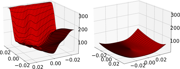
Figure 3: Hessian loss landscapes for deterministic (left) and noisy (right) model, computed using PyHessian.

For establishing a fair set of baselines, we used the following implementations and prescribed tuning parameters for the other models that we considered.

• Exponential RNN. We used the following implementation: https://github.com/Lezcano/expRNN. We used the default parameters. We trained the model, with hidden dimension $d_{h}=128$, for $100$ epochs.

• CoRNN. We used the following implementation, provided as part of the Supplementary Material: https://openreview.net/forum?id=F3s69XzWOia. We used the default parameters proposed by the authors for training the model with hidden dimension $d_{h}=128$. We trained the model for $100$ epochs with learning rate decay at epoch 90.

• Lipschitz RNN. We used the following implementation, provided as part of the Supplementary Material: https://openreview.net/forum?id=-N7PBXqOUJZ. We used the default parameters proposed by the authors for training the model with hidden dimension $d_{h}=128$. We trained the model for $100$ epochs with learning rate decay at epoch 90.

• Antisymmetric RNN. To our best knowledge, there is no public implementation by the authors for this model. However, the Antisymmetric RNN can be seen as a special case of the Lipschitz RNN or the NRNN, without the stabilizing term $A$ and without noise-injection. We trained this model by using our implementation and the following tuning parameters: $\beta=1.0$, $\gamma=0.001$, lr = $0.002$, $\epsilon=0.01$. We trained the model for $100$ epochs with learning rate decay at epoch 90.

G.2 Additional Results for Permuted Pixel-by-Pixel MNIST Classification

Here we consider the permuted pixel-by-pixel MNIST classification task. This task sequentially presents a scrambled sequence of the $784$ pixels to the model and uses the final hidden state to predict the class membership probability of the input image.

Table 5 shows the average test accuracy (evaluated for models that are trained with 10 different seed values). Here we present results for white noise and salt and pepper (S&P) perturbations. Again, the NRNNs show an improved resilience to input perturbations. Figure 4 summarizes the performance of different models with respect to white noise and salt and pepper perturbations.

Table 5: Robustness w.r.t. white noise ($\sigma$) and S&P ($\alpha$) perturbations on the permuted MNIST task.

Name	clean	$\sigma=0.1$	$\sigma=0.2$	$\sigma=0.3$	$\alpha=0.03$	$\alpha=0.05$	$\alpha=0.1$
Antisymmetric RNN [10]	92.8%	92.4%	89.5%	81.9%	90.5%	87.9%	72.6%
CoRNN [65]	96.05%	65.1%	38.25%	29.1%	84.8%	73.8%	52.6%
Exponential RNN [46]	93.3%	90.6%	78.4%	61.6%	80.4%	70.6%	51.6%
Lipschitz RNN [20]	95.9%	95.4%	93.5%	83.7%	93.7%	90.2%	70.8%
NRNN (mult./add. noise: 0.02/0.02)	94.9%	94.8%	94.6%	94.3%	94.0%	93.1%	88.6%
NRNN (mult./add. noise: 0.02/0.05)	94.7%	94.6%	94.6%	94.4%	94.0%	93.2%	90.5%

\begin{overpic}[width=433.62pt]{figs/pmnist_white.pdf} \put(-6.0,15.0){\rotatebox{90.0}{test accuracy}} \put(42.0,-3.0){{amount of noise}} \end{overpic}

(a) White noise perturbations.

\begin{overpic}[width=433.62pt]{figs/pmnist_sp.pdf} \put(42.0,-3.0){{amount of noise}} \end{overpic}

(b) Salt and pepper perturbations.

Figure 4: Test accuracy for the permuted MNIST task as function of the strength of input perturbations.

References

- [1] Alnur Ali, Edgar Dobriban, and Ryan Tibshirani. The implicit regularization of stochastic gradient flow for least squares. In International Conference on Machine Learning, pages 233–244. PMLR, 2020.
- [2] Ludwig Arnold, W Kliemann, and E Oeljeklaus. Lyapunov exponents of linear stochastic systems. In Lyapunov exponents, pages 85–125. Springer, 1986.
- [3] Ludwig Arnold and Wolfgang Kliemann. Large deviations of linear stochastic differential equations. In Stochastic differential systems, pages 115–151. Springer, 1987.
- [4] Raman Arora, Peter Bartlett, Poorya Mianjy, and Nathan Srebro. Dropout: Explicit forms and capacity control. In International Conference on Machine Learning, pages 351–361. PMLR, 2021.
- [5] Omri Azencot, N Benjamin Erichson, Vanessa Lin, and Michael W. Mahoney. Forecasting sequential data using consistent Koopman autoencoders. In International Conference on Machine Learning, pages 475–485. PMLR, 2020.
- [6] Kaushik Balakrishnan and Devesh Upadhyay. Deep adversarial Koopman model for reaction-diffusion systems. arXiv preprint arXiv:2006.05547, 2020.
- [7] Chris M Bishop. Training with noise is equivalent to Tikhonov regularization. Neural Computation, 7(1):108–116, 1995.
- [8] Yurii Nikolaevich Blagoveshchenskii and Mark Iosifovich Freidlin. Some properties of diffusion processes depending on a parameter. In Doklady Akademii Nauk, volume 138, pages 508–511. Russian Academy of Sciences, 1961.
- [9] Alexander Camuto, Matthew Willetts, Umut Simsekli, Stephen J Roberts, and Chris C Holmes. Explicit regularisation in Gaussian noise injections. In Advances in Neural Information Processing Systems, volume 33, pages 16603–16614, 2020.
- [10] Bo Chang, Minmin Chen, Eldad Haber, and Ed H. Chi. AntisymmetricRNN: A dynamical system view on recurrent neural networks. In International Conference on Learning Representations, 2019.
- [11] Minmin Chen, Jeffrey Pennington, and Samuel Schoenholz. Dynamical isometry and a mean field theory of RNNs: Gating enables signal propagation in recurrent neural networks. In International Conference on Machine Learning, pages 873–882. PMLR, 2018.
- [12] Ricky TQ Chen, Yulia Rubanova, Jesse Bettencourt, and David K Duvenaud. Neural ordinary differential equations. In Advances in Neural Information Processing Systems, pages 6571–6583, 2018.
- [13] Zhengdao Chen, Jianyu Zhang, Martin Arjovsky, and Léon Bottou. Symplectic recurrent neural networks. In International Conference on Learning Representations, 2019.
- [14] S. Das and O. Olurotimi. Noisy recurrent neural networks: the continuous-time case. IEEE Transactions on Neural Networks, 9(5):913–936, 1998.
- [15] Michal Derezinski, Feynman T Liang, and Michael W Mahoney. Exact expressions for double descent and implicit regularization via surrogate random design. In Advances in Neural Information Processing Systems, volume 33, pages 5152–5164, 2020.
- [16] Adji Bousso Dieng, Rajesh Ranganath, Jaan Altosaar, and David Blei. Noisin: Unbiased regularization for recurrent neural networks. In International Conference on Machine Learning, pages 1252–1261. PMLR, 2018.
- [17] Akshunna S. Dogra and William Redman. Optimizing neural networks via Koopman operator theory. In Advances in Neural Information Processing Systems, volume 33, pages 2087–2097, 2020.
- [18] Melikasadat Emami, Mojtaba Sahraee-Ardakan, Parthe Pandit, Sundeep Rangan, and Alyson K Fletcher. Implicit bias of linear RNNs. In Proceedings of the 38th International Conference on Machine Learning, volume 139, pages 2982–2992. PMLR, 2021.
- [19] Rainer Engelken, Fred Wolf, and LF Abbott. Lyapunov spectra of chaotic recurrent neural networks. arXiv preprint arXiv:2006.02427, 2020.
- [20] N. Benjamin Erichson, Omri Azencot, Alejandro Queiruga, Liam Hodgkinson, and Michael W. Mahoney. Lipschitz recurrent neural networks. In International Conference on Learning Representations, 2021.
- [21] N Benjamin Erichson, Michael Muehlebach, and Michael W Mahoney. Physics-informed autoencoders for Lyapunov-stable fluid flow prediction. arXiv preprint arXiv:1905.10866, 2019.
- [22] Wei Fang. Adaptive timestepping for SDEs with non-globally Lipschitz drift. PhD thesis, University of Oxford, 2019.
- [23] Wei Fang, Michael B Giles, et al. Adaptive Euler–Maruyama method for SDEs with nonglobally Lipschitz drift. Annals of Applied Probability, 30(2):526–560, 2020.
- [24] Marco Fraccaro, Søren Kaae Sø nderby, Ulrich Paquet, and Ole Winther. Sequential neural models with stochastic layers. In Advances in Neural Information Processing Systems, volume 29, 2016.
- [25] Mark Iosifovich Freidlin and Alexander D Wentzell. Random Perturbations of Dynamical Systems. Springer, 1998.
- [26] J.F.L. Gall. Brownian Motion, Martingales, and Stochastic Calculus. Graduate Texts in Mathematics. Springer International Publishing, 2016.
- [27] D. F. Gleich and M. W. Mahoney. Anti-differentiating approximation algorithms: A case study with min-cuts, spectral, and flow. In Proceedings of the 31st International Conference on Machine Learning, pages 1018–1025, 2014.
- [28] Ary L Goldberger, Luis AN Amaral, Leon Glass, Jeffrey M Hausdorff, Plamen Ch Ivanov, Roger G Mark, Joseph E Mietus, George B Moody, Chung-Kang Peng, and H Eugene Stanley. Physiobank, physiotoolkit, and physionet: components of a new research resource for complex physiologic signals. Circulation, 101(23):e215–e220, 2000.
- [29] Chengyue Gong, Tongzheng Ren, Mao Ye, and Qiang Liu. Maxup: Lightweight adversarial training with data augmentation improves neural network training. In Proceedings of the IEEE/CVF Conference on Computer Vision and Pattern Recognition, pages 2474–2483, 2021.
- [30] Samuel Greydanus, Misko Dzamba, and Jason Yosinski. Hamiltonian neural networks. In Advances in Neural Information Processing Systems, volume 32, 2019.
- [31] Eldad Haber and Lars Ruthotto. Stable architectures for deep neural networks. Inverse Problems, 34(1):014004, 2017.
- [32] Desmond J Higham, Xuerong Mao, and Andrew M Stuart. Strong convergence of Euler-type methods for nonlinear stochastic differential equations. SIAM Journal on Numerical Analysis, 40(3):1041–1063, 2002.
- [33] Liam Hodgkinson, Chris van der Heide, Fred Roosta, and Michael W Mahoney. Stochastic continuous normalizing flows: Training SDEs as ODEs. In Uncertainty in Artificial Intelligence (UAI), 2021.
- [34] Gao Huang, Yu Sun, Zhuang Liu, Daniel Sedra, and Kilian Q Weinberger. Deep networks with stochastic depth. In European Conference on Computer Vision, pages 646–661. Springer, 2016.
- [35] Martin Hutzenthaler and Arnulf Jentzen. Numerical approximations of stochastic differential equations with non-globally Lipschitz continuous coefficients, volume 236. American Mathematical Society, 2015.
- [36] Martin Hutzenthaler, Arnulf Jentzen, Peter E Kloeden, et al. Strong convergence of an explicit numerical method for SDEs with nonglobally Lipschitz continuous coefficients. The Annals of Applied Probability, 22(4):1611–1641, 2012.
- [37] Kam-Chuen Jim, C Lee Giles, and Bill G Horne. An analysis of noise in recurrent neural networks: Convergence and generalization. IEEE Transactions on Neural Networks, 7(6):1424–1438, 1996.
- [38] Anil Kag, Ziming Zhang, and Venkatesh Saligrama. RNNs incrementally evolving on an equilibrium manifold: A panacea for vanishing and exploding gradients? In International Conference on Learning Representations, 2020.
- [39] Ioannis Karatzas and Steven E Shreve. Brownian Motion. Springer, 1998.
- [40] Nitish Shirish Keskar, Dheevatsa Mudigere, Jorge Nocedal, Mikhail Smelyanskiy, and Ping Tak Peter Tang. On large-batch training for deep learning: Generalization gap and sharp minima. arXiv preprint arXiv:1609.04836, 2016.
- [41] Hassan K Khalil and Jessy W Grizzle. Nonlinear Systems, volume 3. Prentice hall Upper Saddle River, NJ, 2002.
- [42] Patrick Kidger, James Morrill, James Foster, and Terry Lyons. Neural controlled differential equations for irregular time series. In Advances in Neural Information Processing Systems, volume 33, pages 6696–6707, 2020.
- [43] Peter E Kloeden and Eckhard Platen. Numerical Solution of Stochastic Differential Equations, volume 23. Springer Science & Business Media, 2013.
- [44] Hiroshi Kunita. Stochastic differential equations and stochastic flows of diffeomorphisms. In Ecole d’été de Probabilités de Saint-Flour XII-1982, pages 143–303. Springer, 1984.
- [45] Quoc V Le, Navdeep Jaitly, and Geoffrey E Hinton. A simple way to initialize recurrent networks of rectified linear units. arXiv preprint arXiv:1504.00941, 2015.
- [46] Mario Lezcano-Casado and David Martınez-Rubio. Cheap orthogonal constraints in neural networks: A simple parametrization of the orthogonal and unitary group. In International Conference on Machine Learning, pages 3794–3803, 2019.
- [47] Yunzhu Li, Hao He, Jiajun Wu, Dina Katabi, and Antonio Torralba. Learning compositional Koopman operators for model-based control. In International Conference on Learning Representations, 2019.
- [48] Soon Hoe Lim. Understanding recurrent neural networks using nonequilibrium response theory. J. Mach. Learn. Res., 22:47–1, 2021.
- [49] Xuanqing Liu, Tesi Xiao, Si Si, Qin Cao, Sanjiv Kumar, and Cho-Jui Hsieh. How does noise help robustness? Explanation and exploration under the neural SDE framework. In Proceedings of the IEEE/CVF Conference on Computer Vision and Pattern Recognition, pages 282–290, 2020.
- [50] Yiping Lu, Aoxiao Zhong, Quanzheng Li, and Bin Dong. Beyond finite layer neural networks: Bridging deep architectures and numerical differential equations. In International Conference on Machine Learning, pages 3276–3285. PMLR, 2018.
- [51] Michael Lutter, Christian Ritter, and Jan Peters. Deep Lagrangian networks: Using physics as model prior for deep learning. arXiv preprint arXiv:1907.04490, 2019.
- [52] Chao Ma, Stephan Wojtowytsch, and Lei Wu. Towards a mathematical understanding of neural network-based machine learning: What we know and what we don’t. arXiv preprint arXiv:2009.10713, 2020.
- [53] M. W. Mahoney. Approximate computation and implicit regularization for very large-scale data analysis. In Proceedings of the 31st ACM Symposium on Principles of Database Systems, pages 143–154, 2012.
- [54] M. W. Mahoney and L. Orecchia. Implementing regularization implicitly via approximate eigenvector computation. In Proceedings of the 28th International Conference on Machine Learning, pages 121–128, 2011.
- [55] Simon JA Malham and Anke Wiese. An introduction to SDE simulation. arXiv preprint arXiv:1004.0646, 2010.
- [56] Xuerong Mao. Exponential Stability of Stochastic Differential Equations. Marcel Dekker, 1994.
- [57] Xuerong Mao. Stochastic Differential Equations and Applications. Elsevier, 2007.
- [58] John Miller and Moritz Hardt. Stable recurrent models. arXiv preprint arXiv:1805.10369, 2018.
- [59] Jeremy Morton, Freddie D Witherden, and Mykel J Kochenderfer. Deep variational Koopman models: Inferring Koopman observations for uncertainty-aware dynamics modeling and control. arXiv preprint arXiv:1902.09742, 2019.
- [60] Hyeonwoo Noh, Tackgeun You, Jonghwan Mun, and Bohyung Han. Regularizing deep neural networks by noise: Its interpretation and optimization. In Advances in Neural Information Processing Systems, pages 5109–5118, 2017.
- [61] Shaowu Pan and Karthik Duraisamy. Physics-informed probabilistic learning of linear embeddings of nonlinear dynamics with guaranteed stability. SIAM Journal on Applied Dynamical Systems, 19(1):480–509, 2020.
- [62] Razvan Pascanu, Tomas Mikolov, and Yoshua Bengio. On the difficulty of training recurrent neural networks. In International Conference on Machine Learning, pages 1310–1318. PMLR, 2013.
- [63] Tomaso Poggio, Kenji Kawaguchi, Qianli Liao, Brando Miranda, Lorenzo Rosasco, Xavier Boix, Jack Hidary, and Hrushikesh Mhaskar. Theory of deep learning III: Explaining the non-overfitting puzzle. arXiv preprint arXiv:1801.00173, 2017.
- [64] Alejandro F Queiruga, N Benjamin Erichson, Dane Taylor, and Michael W Mahoney. Continuous-in-depth neural networks. arXiv preprint arXiv:2008.02389, 2020.
- [65] T. Konstantin Rusch and Siddhartha Mishra. Coupled oscillatory recurrent neural network (coRNN): An accurate and (gradient) stable architecture for learning long time dependencies. In International Conference on Learning Representations, 2021.
- [66] Simo Särkkä and Arno Solin. Applied Stochastic Differential Equations, volume 10. Cambridge University Press, 2019.
- [67] Shai Shalev-Shwartz and Shai Ben-David. Understanding Machine Learning: From Theory to Algorithms. Cambridge University Press, 2014.
- [68] Samuel L Smith, Benoit Dherin, David GT Barrett, and Soham De. On the origin of implicit regularization in stochastic gradient descent. arXiv preprint arXiv:2101.12176, 2021.
- [69] Jure Sokolić, Raja Giryes, Guillermo Sapiro, and Miguel RD Rodrigues. Generalization error of deep neural networks: Role of classification margin and data structure. In 2017 International Conference on Sampling Theory and Applications (SampTA), pages 147–151. IEEE, 2017.
- [70] Jure Sokolić, Raja Giryes, Guillermo Sapiro, and Miguel RD Rodrigues. Robust large margin deep neural networks. IEEE Transactions on Signal Processing, 65(16):4265–4280, 2017.
- [71] David Stutz, Matthias Hein, and Bernt Schiele. Disentangling adversarial robustness and generalization. In Proceedings of the IEEE Conference on Computer Vision and Pattern Recognition, pages 6976–6987, 2019.
- [72] Qi Sun, Yunzhe Tao, and Qiang Du. Stochastic training of residual networks: A differential equation viewpoint. arXiv preprint arXiv:1812.00174, 2018.
- [73] Christian Szegedy, Wojciech Zaremba, Ilya Sutskever, Joan Bruna, Dumitru Erhan, Ian Goodfellow, and Rob Fergus. Intriguing properties of neural networks. arXiv preprint arXiv:1312.6199, 2013.
- [74] Naoya Takeishi, Yoshinobu Kawahara, and Takehisa Yairi. Learning Koopman invariant subspaces for dynamic mode decomposition. In Proceedings of the 31st International Conference on Neural Information Processing Systems, pages 1130–1140, 2017.
- [75] Sachin S Talathi and Aniket Vartak. Improving performance of recurrent neural network with ReLU nonlinearity. arXiv preprint arXiv:1511.03771, 2015.
- [76] Peter Toth, Danilo J Rezende, Andrew Jaegle, Sébastien Racanière, Aleksandar Botev, and Irina Higgins. Hamiltonian generative networks. In International Conference on Learning Representations, 2019.
- [77] Belinda Tzen and Maxim Raginsky. Neural stochastic differential equations: Deep latent Gaussian models in the diffusion limit. arXiv preprint arXiv:1905.09883, 2019.
- [78] Ryan Vogt, Maximilian Puelma Touzel, Eli Shlizerman, and Guillaume Lajoie. On Lyapunov exponents for RNNs: Understanding information propagation using dynamical systems tools. arXiv preprint arXiv:2006.14123, 2020.
- [79] Colin Wei, Sham Kakade, and Tengyu Ma. The implicit and explicit regularization effects of dropout. In Proceedings of the 37th International Conference on Machine Learning, pages 10181–10192, 2020.
- [80] Colin Wei and Tengyu Ma. Data-dependent sample complexity of deep neural networks via Lipschitz augmentation. In Advances in Neural Information Processing Systems, volume 32, 2019.
- [81] E Weinan. A proposal on machine learning via dynamical systems. Communications in Mathematics and Statistics, 5(1):1–11, 2017.
- [82] Huan Xu and Shie Mannor. Robustness and generalization. Machine Learning, 86(3):391–423, 2012.
- [83] Yibo Yang, Jianlong Wu, Hongyang Li, Xia Li, Tiancheng Shen, and Zhouchen Lin. Dynamical system inspired adaptive time stepping controller for residual network families. Proceedings of the AAAI Conference on Artificial Intelligence, 34(04):6648–6655, 2020.
- [84] Zhewei Yao, Amir Gholami, Qi Lei, Kurt Keutzer, and Michael W. Mahoney. Hessian-based analysis of large batch training and robustness to adversaries. In Advances in Neural Information Processing Systems, pages 4954–4964, 2018.
- [85] Wojciech Zaremba, Ilya Sutskever, and Oriol Vinyals. Recurrent neural network regularization. arXiv preprint arXiv:1409.2329, 2014.
- [86] Chiyuan Zhang, Samy Bengio, Moritz Hardt, Benjamin Recht, and Oriol Vinyals. Understanding deep learning (still) requires rethinking generalization. Communications of the ACM, 64(3):107–115, 2021.
- [87] Huishuai Zhang, Da Yu, Mingyang Yi, Wei Chen, and Tie-yan Liu. Stability and convergence theory for learning ResNet: A full characterization. 2019.
- [88] Jingfeng Zhang, Bo Han, Laura Wynter, Bryan Kian Hsiang Low, and Mohan Kankanhalli. Towards robust ResNet: A small step but a giant leap. In Proceedings of the Twenty-Eighth International Joint Conference on Artificial Intelligence, 2019.
- [89] Jingyu Zhao, Feiqing Huang, Jia Lv, Yanjie Duan, Zhen Qin, Guodong Li, and Guangjian Tian. Do RNN and LSTM have long memory? In International Conference on Machine Learning, pages 11365–11375. PMLR, 2020.
- [90] Yaofeng Desmond Zhong, Biswadip Dey, and Amit Chakraborty. Symplectic ODE-Net: Learning Hamiltonian dynamics with control. In International Conference on Learning Representations, 2019.