Physical limits in the Color Dipole Model Bounds

Abstract

The ratio of the cross sections for the transversely and longitudinally virtual photon polarizations, $\sigma^{\gamma^{*}p}_{L/T}$, at high photon-hadron energy scattering is studied. I investigate the relationship between the gluon distribution obtained using the color dipole model and standard gluons obtained from the Dokshitzer-Gribov-Lipatov-Altarelli-Parisi (DGLAP) evolution and the Altarelli-Martinelli equations. It is shown that the color dipole bounds are dependent on the gluon distribution behavior. This behavior is considered by the expansion and Laplace transform methods. Numerical calculations and comparison with the color dipole model (CDM) bounds can indicate the range of validity of this method at small dipole sizes, $r\sim 1/Q{\ll}1/Q_{s}$.

.1 1. Introduction

Dipole model provides a convenient description of deep inelastic scattering (DIS) at small $x$. In this region, partons in the proton form a dense system. Processes such as mutual interaction and recombination leads to the saturation of the total cross section. We know that the DIS cross section is factorized into a light-cone wave function. As the virtual photon splits up into a quark-antiquark pair (dipole). Usually, this contribution ($\gamma^{*}{\rightarrow}q\overline{q}$) is defined as a convolution of the infinite momentum frame wave function with the pQCD calculable coefficient functions. These coefficient functions describing the short distance propagation of the particles between two virtual photon vertices. Many of experimental provided at HERA have been analysis in terms of this model which the dipole picture acts like a quark-antiquark dipole [1-4]. We need to know that the lifetime of the fluctuation of the photon into the color dipole is much larger than the typical timescale of the dipole-proton interaction [5]. In this reference frame, the photon splits into $q\overline{q}$-dipole and then interacts with proton as $q\overline{q}$ lifetime is about $1/x$ times longer than time of interaction with proton.
The saturation region is approached when the reaction is mediated by multi-gluon exchange. This aspect of saturation is closely linked to unitarity. Indeed the growth of the gluon density is slowed down at very small $x$ by gluon -gluon recombination ($g+g\rightarrow g$). In this region the gluon density in hadrons can become nonperturbatively large. It means that it is the regime of gluon saturation. This is the origin of the shadowing correction in pQCD interactions [1]. One of the implementation of multiple scattering in colour dipole model is based on the Glauber-Mueller (GM) eikonal approach [2], which is used in Golec-Biernat-W$\mathrm{\ddot{u}}$sthoff (GBW) model [3]. In this approach the multiple colour dipole scatters are independent of each other which describing the multi-gluon density in the proton by the b-Sat model [4]. As the large saturation effects are required to transition from the hard Pomeron behavior at small dipole sizes to soft Pomeron behavior at large dipole sizes [6].
An effective field theory describing the small-$x$ regime of QCD is the color glass condensate (CGC) [7,8,9]. This model is based on the Balitsky-Kovchegov (BK) [10] non-linear evolution equation and improves the Iancu-Itakura-Munier (IIM) dipole model [11]. The non-linear effects appear in CGC formalism when the gluon density becomes large. Indeed in high energy collisions which $x$ decreases, the number of gluons increase. When gluons are highly coherent at infrared scale, the gluon saturation leads to the Glasma [8,9,10,11]. Indeed the Glasma is matter produced from the CGC after a collision. After the collisions, Glasma is formed in the region between the two sheets of colored glass. At high energy scattering with evolution and recombination of gluon density, one can probes the number of gluons with a given $x$ and transverse momenta $k_{\bot}\leq Q$ as the gluon number is defined by

$$x\frac{dN_{g}}{dx}(Q^{2})=\frac{\alpha_{s}C_{R}}{\pi}\int_{\Lambda^{2}_{QCD}}^{Q^{2}}\frac{dk_{\bot}^{2}}{k_{\bot}^{2}}=\frac{\alpha_{s}C_{R}}{\pi}\ln(\frac{Q^{2}}{\Lambda^{2}_{QCD}})$$ (1)

where $\Lambda_{QCD}$ is the QCD cutoff and $C_{R}$ is the $SU(N_{c})$ Casimir operator [9]. The HERA data collected on the inclusive $\gamma^{*}p$ cross section for $x{\leq}0.01$ indicate a scaling as a function of the ratio $Q^{2}/Q^{2}_{s}(x)$. Which $Q^{2}_{s}(x)=Q_{0}^{2}(x_{0}/x)^{\lambda}$ is the saturation scale with dimensions given by a fixed reference scale $Q_{0}^{2}$ [12]. Indeed saturation scale is a border between dense and dilute gluonic system. For $Q^{2}<Q_{s}^{2}$ the linear evolution is strongly perturbed by nonlinear effects, while for $Q^{2}>Q_{s}^{2}$ the linear evolution is dominated and evolution of parton densities is governed by the DGLAP equations.
The proton structure function $F_{2}$ and the longitudinal structure function $F_{L}$ can be can be written in terms of $\gamma^{*}p$ cross section as follows

$$F_{2}(x,Q^{2}) = \frac{Q^{2}}{4\pi^{2}\alpha_{em}}[\sigma_{L}^{\gamma^{*}p}(x,Q^{2})+\sigma_{T}^{\gamma^{*}p}(x,Q^{2})]$$ (2)

$$F_{L}(x,Q^{2}) = \frac{Q^{2}}{4\pi^{2}\alpha_{em}}\sigma_{L}^{\gamma^{*}p}(x,Q^{2})$$ (3)

where $\alpha_{EM}$ is the electromagnetic fine structure constant. Here the subscripts $L$ and $T$ denote the longitudinal and transverse polarizations of the virtual photon. The reduced cross section $\sigma_{r}$ is expressed in terms of the inclusive proton structure function $F_{2}$ and $F_{L}$ as

$$\sigma_{r}(x,y,Q^{2})=F_{2}(x,Q^{2})-\frac{y^{2}}{1+(1-y)^{2}}F_{L}(x,Q^{2})$$ (4)

where $Q^{2}$ is the virtuality of exchanged photon, $\sqrt{s}$ denotes the center of mass energy in $ep$ collisions and $y=Q^{2}/(sx)$ is the inelasticity variable.
The total cross section behavior in some literatures [3,13] is based on a logarithmic behavior in $x$ which do not violate unitarity. This behavior has been supplemented by unitarity correction. In accordance with the Froissart predictions [14], authors in Ref.[15] have suggested a parameterization of the structure function $F_{2}\leq{\ln^{2}(1/x)}$ at large $s$. This parameterization implies that its growth is limited by the Froissart bound as Bjorken $x{\rightarrow}0$. This parameterization will be important in treatments of ultra-high energy processes. Further investigations of the high-energy limit of QCD at small $x$ provide valuable information about the unitarity limits of QCD and parton saturation effects at future experiments such as an Electron-Ion Collider (EIC) [16], and also the large Hadron Electron collider (LHeC) [17,18,19] and the Future Circular Collider program (FCC-eh)[20]. Also some theoretical analysis at low $x$ have considered the longitudinal structure function $F_{L}(x,Q^{2})$ to describe process [21,22,23].
The paper is organized as follows. In sect.2, we give a summary about the color dipole model. This section reviews the relevant formulae of the dipole picture. We will study the color dipole model bounds with respect to the proton structure function $F_{2}$ at low values of $x$ in section 3. It is the purpose of this paper to predict the behavior of the color dipole bounds at large $Q^{2}$ values at leading order and next-to-leading order approximations. I will attempt to preserve analysis of Altarelli-Martinelli equation and its solution in DGLAP framework for very small dipoles. In the following the Laplace transform method of the gluon distribution function with respect to the transversal and longitudinal structure functions, which both obey the Froissart boundary conditions, in the LO and NLO approximations at low values of $x$ are discussed. Explicit expressions for the Wilson coefficients at the LO are given as well and at the NLO are given for each $Q^{2}$ values for simplicity. These parameters at LO and NLO are compared with bounds in the color dipole model. Section 4 contains the results and discussions. Numerical results for the extracted these parameters in the expansion method and Laplace transform method, together with comparisons with the color dipole bounds are presented in this section. Also the $W^{2}$ dependence of the extracted parameters is discussed (where $W^{2}$ is the energy in the photon-proton center of mass). Conclusions and summary are summarized on Sec.5. Three Appendices contain results used in the main text. In Appendix A the gluon density is discussed with respect to expansion at distinct points of expansion. Appendix B explains the steps for obtaining the gluon density by Laplace transform method. The most cumbersome expressions for the parameterization of the longitudinal structure function at LO and NLO approximations are relegated to Appendix C.

.2 2. A Short Theoretical Input

In this section we briefly present the theoretical part of the color dipole model. For small values of the Bjorken variable $x$, the correct degrees of freedom in the high energy $\gamma^{*}p$ scattering ($\gamma^{*}$ emitted by the incident electron) are given by $q\overline{q}$ colorless dipoles [1]. In the dipole picture, the $\gamma^{*}p$ interaction process can be described as follows that first the virtual photon splits into a $q\overline{q}$ colorless dipole. Then quark and antiquark interact with proton through radiant gluons. In the leading order, the generic structure of the $(q\overline{q})p$ is well described by two-gluon exchange [4]. In deep inelastic scattering (DIS), the small-$x$ saturation means that the partons in the proton form a dense system. This system with mutual interaction and recombination leads to the saturation of the cross section [24]. In the saturation region, the single-gluon exchange changes into multi-gluon exchange. This process also can be extended to the next-to-leading order (NLO) corrections as described in Refs.[25,26]. In Ref.[26] authors discussed the corresponding corrections in the $\gamma^{*}$ Fock state by adding a new $q\overline{q}g$ component to the $q\overline{q}$-state.
Within the dipole framework of the $\gamma^{*}p$ scattering

$$\sigma_{L,T}^{\gamma^{*}p}(x,Q^{2})=\int{d^{2}\mathbf{r}}\int dz\psi^{*}(Q,r,z)\hat{\sigma}(x,r)\psi(Q,r,z).$$ (5)

Indeed the scattering of the virtual photon on the proton can be conceived as a virtual photon fluctuation into a quark-antiquark pair, then the produced quark-antiquark dipole interacts with the proton via gluon exchanges [7]. The integrands are given by the squared of the light cone wave functions of the virtual photon and the scattering amplitudes for the dipole cross section. The first integration is so-called dipole representation where transverse momentum $\mathbf{k}_{T}$ is replaced by its Fourier conjugate variable $\mathbf{r}$. Here $r(\equiv|\mathbf{r}|)$ is the fixed transverse separation of the quarks in the $q\overline{q}$ pair. Here the quark (or antiquark) carries a fraction $z$ of the incoming photon light-cone energy ($0<z<1$). The dipole cross section $\sigma(x,r)$ is usually assumed to be independent of $z$ and it is a solution of the generalized BFKL equation [27]. Also it is universal for all flavors and the $x$ dependence of its comes from the QCD evolution effects described by the generalized BFKL equation. The squared wave function of the $q\overline{q}$ Fock states of the virtual photon is given by the following equations

$$|\Psi_{T}(z,r)|^{2} = \frac{6\alpha_{em}}{4\pi^{2}}\sum_{1}^{n_{f}}e_{f}^{2}\{[z^{2}+(1-z)^{2}]\epsilon^{2}K_{1}^{2}(\epsilon{r})$$

$$+m^{2}_{f}K_{1}^{2}(\epsilon{r})\},$$

$$\mathrm{and}~{}~{}~{}~{}~{}~{}~{}~{}~{}$$

$$|\Psi_{L}(z,r)|^{2} = \frac{6\alpha_{em}}{4\pi^{2}}\sum_{1}^{n_{f}}e_{f}^{2}\{4Q^{2}z^{2}(1-z)^{2}K_{0}^{2}(\epsilon{r})\},$$ (6)

where $n_{f}$ is the number of active quark flavor. In the above equations $\epsilon^{2}=z(1-z)Q^{2}+m_{f}^{2}$ and $m_{f}$ is the quark mass. $e_{f}$ is the quark charge and the functions $K_{0,1}$ are the Bessel-McDonald functions. The mass of $q\overline{q}$ dipole is realized by $M^{2}_{q\overline{q}}=\frac{\overrightarrow{k_{\bot}}^{2}}{z(1-z)}$. Which the transverse momentum $\overrightarrow{k_{\bot}}$ is introduced into four momenta of the quark and antiquark. If the three momenta $\overrightarrow{q}=\overrightarrow{k}+\overrightarrow{k}^{\prime}$ is defined in the direction of the $z$-axis of a coordinate system, then the quark and antiquark momenta represented by

$$\overrightarrow{k}=z\overrightarrow{q}+{\overrightarrow{k_{\bot}}},$$

$$\overrightarrow{k}^{\prime}=(1-z)\overrightarrow{q}-{\overrightarrow{k_{\bot}}}$$ (7)

where $\overrightarrow{k_{\bot}}.\overrightarrow{q}=0$. With respect to the center-of-mass energy $W$, the restriction on masses of the $q\overline{q}$ states is defined by

$$\frac{M^{2}_{q\overline{q}}}{W^{2}}\ll 0.1,$$ (8)

where the Bjorken variable $x{\cong}\frac{Q^{2}}{W^{2}}{\ll}0.1$. In this approach the photoabsorption cross section can be factorized in the following form

$$\sigma_{L,T}^{\gamma^{*}p}(x,Q^{2}) = \int dzd^{2}\mathbf{r}_{\bot}|\Psi_{\gamma}^{L,T}(\mathbf{r}_{\bot},z(1-z),Q^{2})|^{2}$$ (9)

$${\times}\widehat{\sigma}_{q\overline{q}}(\mathbf{r}_{\bot},W^{2}),$$

where $\sigma_{q\overline{q}}(\mathbf{r}_{\bot},W^{2})$ is the color-dipole cross-section

$$\widehat{\sigma}_{(q\overline{q})p}(\mathbf{r}_{\bot},W^{2}) = \int d^{2}{\overrightarrow{\ell}}_{\bot}\widetilde{\sigma}_{(q\overline{q})p}({\overrightarrow{\ell}}_{\bot}^{2},W^{2})$$ (10)

$${\times}(1-e^{-i{\overrightarrow{\ell}}_{\bot}{\overrightarrow{r}}_{\bot}}),$$

which the variable $\mathbf{r}_{\bot}$ determines the transverse $q\overline{q}$-separation variable and ${\overrightarrow{\ell}}_{\bot}$ stands for the transverse momentum of the absorbed gluon. In the above integral (i.e., Eq.(10)), the first term is associated with the gluon transverse momentum distribution and the second term is the QCD gauge theory structure [28,29].
On the other hand, the dipole cross section was proposed to have the following form [3,21]

$$\widehat{\sigma}_{(q\overline{q})p}(x,r)=\sigma_{0}\{1-\exp(-\frac{\pi^{2}r^{2}\alpha_{s}(\mu^{2})xg(x,\mu^{2})}{3\sigma_{0}})\},$$ (11)

where $\sigma_{0}$ is a parameter of the model and determined from a fit to small-$x$ data. This form of the dipole cross section imposes the unitarity condition at large dipole sizes $r$ as $\widehat{\sigma}_{(q\overline{q})p}{\leq}\sigma_{0}$. For small dipole sizes $r$, the dipole cross section is in agreement with the phenomenon of color transparency resulting from pQCD. The right-hand side of Eq.(10) is proportional to Eq.(11) in the small-$r$ region as [28]

$$\alpha_{s}(Q^{2})xg(x,Q^{2})=\frac{3}{4\pi}\int d{\overrightarrow{\ell}}_{\bot}^{2}{\overrightarrow{\ell}}_{\bot}^{2}\widetilde{\sigma}_{(q\overline{q})p}({\overrightarrow{\ell}}_{\bot}^{2},W^{2}).$$ (12)

Plotting the experimental data for $\sigma^{\gamma^{*}p}$ (where $\sigma^{\gamma^{*}p}=\sigma_{T}^{\gamma^{*}p}+\sigma_{L}^{\gamma^{*}p}=4\pi^{2}\alpha_{em}F_{2}/Q^{2}$) as a function of the scaling variable $\eta(W^{2},Q^{2})=\frac{Q^{2}+m^{2}_{0}}{\Lambda^{2}_{sat}(W^{2})}$ shows a unique behavior as

$$\sigma^{\gamma^{*}p}~{}{\sim}~{}\sigma^{(\infty)}\begin{cases}\frac{1}{\eta(W^{2},Q^{2})},~{}~{}~{}~{}~{}~{}~{}\mathrm{for}~{}\eta\gg 1\\ \ln\frac{1}{\eta(W^{2},Q^{2})},~{}~{}~{}~{}\mathrm{for}~{}\eta\ll 1.\\ \end{cases}$$ (13)

Here the quantity $\sigma^{(\infty)}$ is independent of the photon energy, and $\Lambda_{sat}(W^{2})$ is the saturation scale. The color transparency or saturation of the dipole cross section depend on that $Q^{2}{\gg}\Lambda_{sat}^{2}(W^{2})$ or $Q^{2}{\ll}\Lambda_{sat}^{2}(W^{2})$ respectively. Refs.[28] and [29] show that the saturation scale is defined by

$$\Lambda^{2}_{sat}(W^{2})=\frac{\pi}{\sigma^{(\infty)}}\int d{\overrightarrow{\ell^{\prime}}}_{\bot}^{2}{\overrightarrow{\ell^{\prime}}}_{\bot}^{2}\widetilde{\sigma}_{(q\overline{q})_{L}^{J=1}}({\overrightarrow{\ell^{\prime}}}_{\bot}^{2},W^{2}),$$ (14)

which is fixed spin $J=1$ and $\ell^{\prime}$ is defined into the gluon transverse momentum. Also the light-cone variable $z$ reads as

$${\overrightarrow{\ell^{\prime}}}_{\bot}^{2}=\frac{{\overrightarrow{\ell}}_{\bot}^{2}}{z(1-z)}.$$

Therefore, the relationship between gluon distribution and saturation scale is expressed in the form

$$\alpha_{s}(Q^{2})xg(x,Q^{2})=\frac{1}{8\pi}\sigma^{(\infty)}\Lambda^{2}_{sat}(W^{2}).$$ (15)

We know that the leading contribution to $F_{2}(x,Q^{2})$ at sufficiently large $Q^{2}$ in terms of the $J=1$ projection becomes

$$F_{2}(x,Q^{2}) = \frac{Q^{2}}{4\pi^{2}\alpha}(\sigma_{\gamma^{*}_{T}p}(W^{2},Q^{2})+\sigma_{\gamma^{*}_{L}p}(W^{2},Q^{2}))$$ (16)

$$=\frac{R_{e^{+}e^{-}}}{36\pi^{2}}(\int d{\overrightarrow{\ell^{\prime}}}_{\bot}^{2}{\overrightarrow{\ell^{\prime}}}_{\bot}^{2}\widetilde{\sigma}_{(q\overline{q})_{T}^{J=1}}({\overrightarrow{\ell^{\prime}}}_{\bot}^{2},W^{2})$$

$$+\frac{1}{2}\int d{\overrightarrow{\ell^{\prime}}}_{\bot}^{2}{\overrightarrow{\ell^{\prime}}}_{\bot}^{2}\widetilde{\sigma}_{(q\overline{q})_{L}^{J=1}}({\overrightarrow{\ell^{\prime}}}_{\bot}^{2},W^{2})),$$

where $R_{e^{+}e^{-}}=3\sum_{f}e_{f}^{2}$. As shown in Ref.[30], the longitudinal and transverse terms on the right-hand side in (16) becomes

$$\int d{\overrightarrow{\ell^{\prime}}}_{\bot}^{2}{\overrightarrow{\ell^{\prime}}}_{\bot}^{2}\widetilde{\sigma}_{(q\overline{q})_{T}^{J=1}}({\overrightarrow{\ell^{\prime}}}_{\bot}^{2},W^{2})$$

$$=\rho\int d{\overrightarrow{\ell^{\prime}}}_{\bot}^{2}{\overrightarrow{\ell^{\prime}}}_{\bot}^{2}\widetilde{\sigma}_{(q\overline{q})_{L}^{J=1}}({\overrightarrow{\ell^{\prime}}}_{\bot}^{2},W^{2}),$$ (17)

The parameter $\rho$ is associated with the enhanced transverse size of $q\overline{q}$ fluctuations in the CDM originating from transverse, $\gamma^{*}_{T}{\rightarrow}q\overline{q}$, and longitudinal, $\gamma^{*}_{L}{\rightarrow}q\overline{q}$, photons. Indeed the $\rho$ parameter describes the ratio of the average transverse momenta $\rho=\frac{<\overrightarrow{k}^{2}_{\bot}>_{L}}{<\overrightarrow{k}^{2}_{\bot}>_{T}}$. It can also be related to the ratio of the effective transverse sizes of the $(q\overline{q})^{J=1}_{L,T}$ states as $\frac{<\overrightarrow{r}^{2}_{\bot}>_{L}}{<\overrightarrow{r}^{2}_{\bot}>_{T}}=\frac{1}{\rho}$. The ratio of the longitudinal to the transversal photoabsorption cross sections is given by

$$R = \frac{\sigma^{\gamma^{*}p}_{L}}{\sigma^{\gamma^{*}p}_{T}}=\frac{1}{2\rho},$$ (18)

where factor 2 originates from the difference in the photon wave functions. In terms of the proton structure functions, $F_{2}(x,Q^{2})$ and $F_{L}(x,Q^{2})$, the ratio becomes

$$F_{L/2} \equiv \frac{F_{L}}{F_{2}}=\frac{1}{1+2\rho}.$$ (19)

The quantity of $\rho$ in previous analysis [28,29,30,31] is considered equal to $1$(i.e., $\rho=1$) and for $Q^{2}\gg\Lambda_{sat}^{2}(W^{2})$ was used the value $\rho=4/3$. The deviation from $\rho=1$ quantifies the deviation between the scatterings of longitudinally polarized versus transversally polarized $q\overline{q}$ fluctuations of the photon. In the large-$Q^{2}$ limit, the structure function (according to Eq.(14)) takes the form

$$F_{2}(x,Q^{2}) = \frac{R_{e^{+}e^{-}}}{36\pi^{3}}\sigma^{(\infty)}\Lambda^{2}_{sat}(W^{2})(\rho+\frac{1}{2}).$$ (20)

The structure function $F_{2}(x,Q^{2})$ in the small $x$ limit in the DIS scheme is proportional to the flavor-singlet quark distribution, $\Sigma(x,Q^{2})$, as

$$F_{2}(x,Q^{2})=\frac{R_{e^{+}e^{-}}}{12}x\Sigma(x,Q^{2}),$$ (21)

which $x\Sigma(x,Q^{2})=n_{f}(xq(x,Q^{2})+x\overline{q}(x,Q^{2}))$. Due to that the sea-quark and gluon distributions have identical dependence on the kinematic variables, therefore they are assumed [28,29,30,31] to be proportional to each other with respect to the $\rho$ parameter as

$$x\Sigma(x,Q^{2})=\frac{8}{3\pi}\alpha_{s}(Q^{2})xg(x,Q^{2})(\rho+\frac{1}{2}).$$ (22)

Consequently the $\rho$ parameter into the singlet structure function and gluon distribution function reads as

$$\rho=\frac{3\pi}{8\alpha_{s}(Q^{2})}\frac{F_{2}^{s}(x,Q^{2})}{G(x,Q^{2})}-\frac{1}{2},$$ (23)

where $F_{2}^{s}(x,Q^{2})=x\Sigma(x,Q^{2})$ and $G(x,Q^{2})=xg(x,Q^{2})$. Indeed Eq.(23) is valid for very small dipoles which it is in agreement with the phenomenon of color transparency resulting from perturbative QCD. Therefore I will obtain the relation between gluon distribution function and dipole cross-section in order to rewrite the ratio of structure functions for the color dipole framework.

.3 3. Model Description

In order to describe the ratio of structure functions it is necessary to make specific methods about the gluon behavior in the color dipole model upon applying the DGLAP evolution. First, I give a simple method for the gluon distribution due to the expansion method at the appropriate points of expansion and contrast this method with other methods that have appeared previously. Then I define the gluon distribution and the proton structure functions according to the parameterization method. Then I analyse the consistency between the Altarelli-Martinelli relation of the gluon distribution and the color dipole model bounds. In the following I define and discuss the $\rho$ parameter in the color dipole picture with respect to the Laplace transform method at LO and NLO approximations. Finally after the parameterization of structure functions are specified, I determined the parameters by rely on the Froissart-bounded parameterization of the DIS structure functions.

.4 3.1. Expansion Method

The authors in Refs.[28-31] have used the same correlation between gluon distribution and derivative of structure function mentioned in Ref.[32] at sufficiently low values of the Bjorken variable $x\simeq Q^{2}/W^{2}{\ll}0.1$. The evolution of the structure function with respect to $\ln{Q^{2}}$ is determined by

$$\frac{\partial F_{2}(x,Q^{2})}{\partial{\ln{Q^{2}}}}\simeq\frac{\alpha_{s}(Q^{2})}{3\pi}\sum_{q}e_{q}^{2}G(2x,Q^{2}).$$ (24)

Also another similar relation for the longitudinal structure function into the gluon density is given as follows [33]

$$F_{L}(x,Q^{2})\simeq\frac{2\alpha_{s}(Q^{2})}{5.9\pi}\sum_{q}e_{q}^{2}G(2.5,Q^{2}).$$ (25)

Eqs.(24) and (25) actually indicates that the structure functions are dependent to the gluon density at low $x$ approximation of the pQCD. That means for $x\simeq Q^{2}/W^{2}{\ll}1$, the photon-proton interaction is dominated by the gluon fusion process via $\gamma^{*}gluon{\rightarrow}q\overline{q}$. In the last years these methods [32,33] were proposed to isolate the gluon density by its expansion around $z=\frac{1}{2}$. One method was proposed in Ref.[34] by the expansion of the gluon density at an arbitrary $z=a$ (For future discussion please see Appendix A), as

$$\frac{\partial F_{2}(x,Q^{2})}{\partial{\ln{Q^{2}}}}\simeq\frac{5\alpha_{s}(Q^{2})}{9\pi}\frac{2}{3}G(\frac{x}{1-a}(\frac{3}{2}-a),Q^{2}).$$ (26)

A similar relationship for the behavior of the longitudinal structure function at low $x$ is also described in Ref.[35] . Therefore the ratio $\rho$ for a point of expansion $a<1$ can be expressed by

$$\rho=\frac{1}{2}[{F_{2}(x,Q^{2})}/{\frac{\partial F_{2}(X,Q^{2})}{\partial{\ln{Q^{2}}}}}-1],$$ (27)

where $X=x\frac{1-a}{\frac{3}{2}-a}$. When the point $a=\frac{1}{2}$ is used, we get the result expressed in the literatures [28-31]. Authors in Ref.[35] showed that according to the expansion method, a general relationship for the longitudinal structure function into the gluon distribution at low values of $x$ and at LO approximation can be obtained by the following form

$$F_{L}(x,Q^{2})=\frac{10\alpha_{s}(Q^{2})}{27\pi}G(\frac{\frac{3}{2}-a}{1-a}x,Q^{2}).$$

Therefore, we can express Eq.(23) in terms of the longitudinal structure function as

$$\rho=\frac{1}{2}[{F_{2}(x,Q^{2})}/F_{L}(X,Q^{2})-1],$$ (28)

which the longitudinal structure function in connection with the Froissart bound at LO and NLO approximations is investigated at Ref.[21]. In another method, the expansion of the longitudinal structure function is described into the high order corrections in Refs.[36,37].

.5 3.2. Parameterization Method

Using a parameterization suggested by authors in Ref.[15] on the proton structure function in a full accordance with the Froissart predictions [14]. The explicit expression for the $F_{2}$ parameterization, which obtained from a combined fit of the H1 and ZEUS collaborations data [38] in a range of the kinematical variables $x$ and $Q^{2}$( $x<0.01$ and $0.15<Q^{2}<3000~{}\mathrm{GeV}^{2}$), is given by the following form

$$F_{2}(x,Q^{2}) = D(Q^{2})(1-x)^{n}\sum_{m=0}^{2}A_{m}(Q^{2})L^{m},$$ (29)

where

$$A_{0}(Q^{2}) = a_{00}+a_{01}{\ln}(1+\frac{Q^{2}}{\mu^{2}}),$$

$$A_{1}(Q^{2}) = a_{10}+a_{11}{\ln}(1+\frac{Q^{2}}{\mu^{2}})+a_{12}{\ln}^{2}(1+\frac{Q^{2}}{\mu^{2}}),$$

$$A_{2}(Q^{2}) = a_{20}+a_{21}{\ln}(1+\frac{Q^{2}}{\mu^{2}})+a_{22}{\ln}^{2}(1+\frac{Q^{2}}{\mu^{2}}),$$

$$D(Q^{2}) = \frac{Q^{2}(Q^{2}+\lambda M^{2})}{(Q^{2}+M^{2})^{2}},$$

$$L^{m} = \ln^{m}(\frac{1}{x}\frac{Q^{2}}{Q^{2}+\mu^{2}}).$$ (30)

Here $M$ and $\mu^{2}$ are the effective mass a scale factor respectively. The additional parameters with their statistical errors are given in Table I.
The point to be considered in Eqs.(24), (25) and (26) is that both $F_{2}$ and $F_{L}$ are related at small $x$ mainly through the gluon density. For this purpose, we thoroughly examine the equations of evolution. According to the LO DGLAP [40] evolution equation for 4 massless quarks the formalism introduced in Refs.[41], the evolution of the proton structure function is given by

$$\mathcal{F}(x,Q^{2})=x\int_{x}^{1}G(z,Q^{2})K_{qg}(\frac{x}{z})\frac{dz}{z^{2}},$$ (31)

where $K_{qg}$ is the $\mathrm{gluon}{\rightarrow}\mathrm{quark}$ splitting in leading order of QCD (For more on other quantities, please see Appendix B). With respect to the Laplace transform method, the analytical equation for the gluon distribution $G(x,Q^{2})$ for massless quarks is given by

$$G(x,Q^{2}) = 3\mathcal{FF}(x,Q^{2})-\frac{\partial{\mathcal{FF}(x,Q^{2})}}{\partial{\ln x}}$$ (32)

$$-\int_{x}^{1}\mathcal{FF}(z,Q^{2})(\frac{x}{z})^{3/2}\big{\{}\frac{6}{\sqrt{7}}\sin[\frac{\sqrt{7}}{2}\ln\frac{z}{x}]$$

$$+2\cos[\frac{\sqrt{7}}{2}\ln\frac{z}{x}]\frac{dz}{z}\big{\}},$$

where

$$\mathcal{FF}(x,Q^{2})=(\frac{\alpha_{s}}{4\pi}\sum_{q}e_{q}^{2})^{-1}\mathcal{F}_{2}(x,Q^{2}),$$ (33)

and

$$\mathcal{F}_{2}(x,Q^{2}){\equiv}\frac{\partial{F_{2}(x,Q^{2})}}{\partial{\ln Q^{2}}}-\frac{\alpha_{s}}{4\pi}x\int_{x}^{1}F_{2}(z,Q^{2})K_{qq}(\frac{x}{z})\frac{dz}{z^{2}}.$$

Therefore the ratio $\rho$ is

$$\rho=\frac{27\pi}{20\alpha_{s}(Q^{2})}\frac{F_{2}(x,Q^{2})(\mathrm{i.e.,Eq.(29)})}{G(x,Q^{2})(\mathrm{i.e.,Eq.(32)})}-\frac{1}{2}.$$ (35)

Indeed the above equation (i.e., Eq.(35)) expressed based on the Froissart-bounded parameterization of $F_{2}(x,Q^{2})$ while Eq.(27) is expressed based on the condition of gluon dominant at low $x$ as gluon carries the $z=a$ fraction from the proton momentum.

.6 3.3. Laplace Transform Method at LO approximation

In the following I developed model due to the Laplace transform method at LO and NLO approximation. The parameterization of the structure functions should satisfy the CDM bounds. In Ref.[21] the longitudinal structure function $F_{L}(x,Q^{2})$ extracted as it follows the Froissart boundary conditions (For more discussion please see Appendix C). Now I want to express a new interpretation for Eq.(23), based on which the ratio $\rho$ will be determined in terms of $F_{2}(x,Q^{2})$ and $F_{L}(x,Q^{2})$ structure functions, both of which follow the Froissart boundary condition. The standard collinear factorization formula for $F_{L}(x,Q^{2})$ at low values of $x$ reads [54]

$$F_{L}(x,Q^{2}) = a_{s}(Q^{2})[(c_{L,q}^{(0)}(x)+a_{s}(Q^{2})c_{L,q}^{(1)}(x)+...)$$ (36)

$${\otimes}F_{2}(x,Q^{2})+<e^{2}>(c_{L,g}^{(0)}(x)$$

$$+a_{s}(Q^{2})c_{L,g}^{(1)}(x)+...){\otimes}G(x,Q^{2})],$$

where $<e^{2}>$ is the average squared charge and the singlet-quark coefficient function is defined by $c_{L,q}^{(n)}=c_{L,ns}^{(n)}+c_{L,ps}^{(n)}$ which decomposed into the non-singlet and pure singlet contribution. Some analytical solutions of the Altarelli-Martinelli [55] equation have been reported in recent years [56-60] with considerable phenomenological success.
Now I use the coordinate transformation in $\upsilon$-space. The longitudinal structure function reads as

$$\mathcal{\widehat{F}}_{L}(\upsilon,Q^{2}) = a_{s}(Q^{2})\int_{0}^{\upsilon}[(\widehat{c}_{L,q}^{(n)}(\upsilon-w)+...)\mathcal{\widehat{F}}_{2}(w,Q^{2})$$

$$+<e^{2}>(\widehat{c}_{L,g}^{(n)}(\upsilon-w)+...)\mathcal{\widehat{G}}(w,Q^{2})]dw,$$

where the functions ${\widehat{f}}(\mathrm{i.e.},~{}\mathcal{\widehat{F}},\widehat{c}~{}\mathrm{and}~{}\mathcal{\widehat{G}})$ are defined by

$$\widehat{f}(\upsilon,Q^{2}){\equiv}\widehat{f}(e^{-\upsilon},Q^{2}).$$

With respect to the Laplace transforms (Please see Appendix B) we have

$$F_{L}(s,Q^{2})=a_{s}(Q^{2})[k(s)F_{2}(s,Q^{2})+h(s)g(s,Q^{2})],$$ (38)

where at LO approximation $h(s)=<e^{2}>c_{L,g}^{(0)}(s)$ and $k(s)=c_{L,q}^{(0)}(s)$. Solving Eq.(38) for $g$, we find that

$$g(s,Q^{2})=\frac{1}{a_{s}(Q^{2})}\frac{F_{L}(s,Q^{2})}{h(s)}-\frac{k(s)}{h(s)}F_{2}(s,Q^{2}).$$ (39)

Then we take the inverse laplace transform as the above equation (i.e., Eq.(39)) can be written as

$$\widehat{G}(\upsilon,Q^{2}) = \frac{1}{a_{s}(Q^{2})}\mathcal{L}^{-1}[F_{L}(s,Q^{2}){h(s)}^{-1}]$$ (40)

$$-\mathcal{L}^{-1}[F_{2}(s,Q^{2})\frac{k(s)}{h(s)}],$$

where $\mathcal{L}^{-1}[g(s,Q^{2});\upsilon]=\widehat{G}(\upsilon,Q^{2})$. Therefore we find that

$$\widehat{G}(\upsilon,Q^{2}) = \frac{1}{a_{s}(Q^{2})}\int_{0}^{\upsilon}\mathcal{\widehat{F}}_{L}(w,Q^{2})\widehat{J}(\upsilon-w)dw$$

$$-\int_{0}^{\upsilon}\mathcal{\widehat{F}}_{2}(w,Q^{2})\widehat{L}(\upsilon-w)dw,$$

where $\widehat{J}(\upsilon)$ and $\widehat{L}(\upsilon)$ are new auxiliary functions, defined by

$$\widehat{J}(\upsilon) {\equiv} \mathcal{L}^{-1}[h^{-1}(s);\upsilon],$$

$$\widehat{L}(\upsilon) {\equiv} \mathcal{L}^{-1}[{k(s)}{h(s)^{-1}};\upsilon].$$ (42)

The calculations of $\widehat{J}(\upsilon)$ and $\widehat{L}(\upsilon)$, using the inverse Laplace transform, are straightforward and are given in terms of the Dirac delta function and its derivatives, as we find that

$$\widehat{J}(\upsilon) = \frac{3}{4n_{f}}\delta(\upsilon)+\frac{5}{8n_{f}}\delta^{\prime}(\upsilon)+\frac{1}{8n_{f}}\delta^{\prime\prime}(\upsilon),$$

$$\widehat{L}(\upsilon) = 2C_{F}(\frac{3}{4n_{f}}\delta(\upsilon)+\frac{1}{4n_{f}}\delta^{\prime}(\upsilon)).$$ (43)

Using the properties of Dirac delta function, we therefore obtain an explicit solution for the gluon distribution in terms of the parameterization of $F_{2}(x,Q^{2})$ [15] and $F_{L}(x,Q^{2})$ [21] by

$$G^{LO}(x,Q^{2}) = \frac{1}{a_{s}(Q^{2})<e^{2}>}[\frac{1}{8n_{f}}x^{2}\frac{{\partial}^{2}}{{\partial}x^{2}}F_{L}^{LO}(x,Q^{2})$$ (44)

$$-\frac{5}{8n_{f}}x\frac{{\partial}}{{\partial}x}F_{L}^{LO}(x,Q^{2})+\frac{3}{4n_{f}}F_{L}^{LO}(x,Q^{2})]$$

$$-\frac{2C_{F}}{<e^{2}>}[-\frac{1}{4n_{f}}x\frac{{\partial}}{{\partial}x}F_{2}(x,Q^{2})$$

$$+\frac{3}{4n_{f}}F_{2}(x,Q^{2})],$$

where the parameterization of $F_{2}$ is given by (29). The explicit expression for the parameterization of $F_{L}$ at the LO approximation is obtained by the following form [21]

$$F_{L}^{\mathrm{LO}}(x,Q^{2}) = (1-x)^{n}\sum_{m=0}^{2}C_{m}(Q^{2})L^{m}.$$ (45)

The coefficient functions and future discussion about the above relation can be found in Appendix C. In this formalism both $F_{2}$ and $F_{L}$ obey the Froissart boundary condition. Therefore we find the ratio $\rho$ with respect to the Laplace transform method at LO approximation by the following form

$$\rho=\frac{27\pi}{20\alpha_{s}(Q^{2})}\frac{\mathrm{Eq}.(29)}{\mathrm{Eq}.(44)}-\frac{1}{2}.$$ (46)

.7 3.4. Laplace Transform Method at NLO approximation

Finally I discuss how the higher-order components of the coefficient functions may affect these bounds. The longitudinal structure function within the NLO approximation in $\upsilon$-space reads as

$$\mathcal{\widehat{F}}_{L}(\upsilon,Q^{2}) = a_{s}(Q^{2})\int_{0}^{\upsilon}[(\widehat{c}_{L,q}^{(0)}(\upsilon-w)+a_{s}(Q^{2}){\times}$$ (47)

$$\widehat{c}_{L,q}^{(1)}(\upsilon-w))\mathcal{\widehat{F}}_{2}(w,Q^{2})+<e^{2}>(\widehat{c}_{L,g}^{(0)}(\upsilon-w)$$

$$+a_{s}(Q^{2})\widehat{c}_{L,g}^{(1)}(\upsilon-w))\mathcal{\widehat{G}}(w,Q^{2})]dw.$$

Then transform the NLO longitudinal structure function into $s$-space is

$$F_{L}(s,Q^{2})=a_{s}(Q^{2})[K(s)F_{2}(s,Q^{2})+H(s)g(s,Q^{2})],$$ (48)

where the coefficient functions at NLO approximation are extended by $H(s)=<e^{2}>[c_{L,g}^{(0)}(s)+a_{s}(Q^{2})c_{L,g}^{(1)}(s)]$ and $K(s)=c_{L,q}^{(0)}(s)+a_{s}(Q^{2})c_{L,q}^{(1)}(s)$. Now the inverse Laplace transforms of the above equation (i.e., Eq.(48)) can be performed in the following form

$$\widehat{G}(\upsilon,Q^{2}) = \frac{1}{a_{s}(Q^{2})}\mathcal{L}^{-1}[\frac{F_{L}(s,Q^{2})}{<e^{2}>}(c_{L,g}^{(0)}(s)$$ (49)

$$+a_{s}(Q^{2})c_{L,g}^{(1)}(s))^{-1}]-\mathcal{L}^{-1}[\frac{F_{2}(s,Q^{2})}{<e^{2}>}$$

$${\times}\frac{c_{L,q}^{(0)}(s)+a_{s}(Q^{2})c_{L,q}^{(1)}(s)}{c_{L,g}^{(0)}(s)+a_{s}(Q^{2})c_{L,g}^{(1)}(s)}].$$

Indeed the gluon distribution at NLO approximation can be represented as

$$\widehat{G}(\upsilon,Q^{2}) = \frac{1}{a_{s}(Q^{2})}\int_{0}^{\upsilon}\mathcal{\widehat{F}}_{L}(w,Q^{2})\widehat{T}(\upsilon-w)dw$$

$$-\int_{0}^{\upsilon}\mathcal{\widehat{F}}_{2}(w,Q^{2})\widehat{U}(\upsilon-w)dw,$$

where

$$\widehat{T}(\upsilon) {\equiv} \mathcal{L}^{-1}[H^{-1}(s);\upsilon],$$

$$\widehat{U}(\upsilon) {\equiv} \mathcal{L}^{-1}[{K(s)}{H(s)^{-1}};\upsilon].$$ (51)

The inverse Laplace transform of the terms $\widehat{T}(\upsilon)$ and $\widehat{U}(\upsilon)$ at NLO approximation are straightforward but they are too lengthy. In the limit case for these terms, the simplest form can be expressed by the following form for $Q^{2}=100~{}\mathrm{GeV}^{2}$ as

$$\widehat{T}(\upsilon) = 0.2200\delta(\upsilon)+0.1630\delta^{\prime}(\upsilon)+0.0320\delta^{\prime\prime}(\upsilon)$$

$$+0.0001e^{-2.0620\upsilon}-0.0036e^{-1.2730\upsilon}$$

$$+0.0250e^{-0.5680\upsilon}+0.0189e^{0.0730\upsilon},$$

$$\widehat{U}(\upsilon) = 0.4980\delta(\upsilon)+0.1580\delta^{\prime}(\upsilon)+0.0381e^{-2.0620\upsilon}$$ (52)

$$+0.0620e^{-1.273\upsilon}+0.0040e^{0.0730\upsilon}-0.0210e^{-\upsilon}$$

$$-0.0160e^{-0.5680\upsilon}-0.0640e^{-4\upsilon}.$$

Therefore an analytical solution for the NLO gluon distribution in terms of the parameterization of $F_{2}(x,Q^{2})$ [15] and $F_{L}(x,Q^{2})$ [21] at NLO approximation at $Q^{2}=100~{}\mathrm{GeV}^{2}$ is obtained by

$$G^{\mathrm{NLO}}(x,Q^{2}) = 268.361\bigg{[}0.0320~{}x^{2}\frac{{\partial}^{2}}{{\partial}x^{2}}F_{L}^{\mathrm{NLO}}(x,Q^{2})-0.1630~{}x\frac{{\partial}}{{\partial}x}F_{L}^{\mathrm{NLO}}(x,Q^{2})+0.2200F_{L}^{\mathrm{NLO}}(x,Q^{2})$$ (53)

$$+\int_{x}^{1}\frac{dz}{z}F_{L}^{\mathrm{NLO}}(z,Q^{2})\bigg{\{}0.0001(\frac{x}{z})^{2.0620}-0.0036(\frac{x}{z})^{1.2720}+0.0250(\frac{x}{z})^{0.5680}+0.0189(\frac{z}{x})^{0.0730}\bigg{\}}\bigg{]}$$

$$-\frac{18}{5}\bigg{[}0.4980~{}F_{2}(x,Q^{2})-0.1580~{}x\frac{{\partial}}{{\partial}x}F_{2}(x,Q^{2})+\int_{x}^{1}\frac{dz}{z}F_{2}(z,Q^{2})\bigg{\{}0.0381(\frac{x}{z})^{2.0620}+0.0620(\frac{x}{z})^{1.2720}$$

$$-0.0160(\frac{x}{z})^{0.5680}+0.0040(\frac{z}{x})^{0.0730}-0.0210(\frac{x}{z})-0.0640(\frac{z}{z})^{4}\bigg{\}}\bigg{]},$$

Therefore, at NLO approximation, the ratio $\rho$ is obtained as follows

$$\rho=\frac{27\pi}{20\alpha_{s}(Q^{2})}\frac{\mathrm{Eq}.(29)}{\mathrm{Eq}.(53)}-\frac{1}{2},$$ (54)

and

$$F_{L/2}^{NLO}=\frac{1}{1+2\rho(\mathrm{Eq}.54)}.$$

The NLO corrections for the dipole factorization of DIS structure functions at low $x$ values have been considered in Ref.[61]. In Ref.[61] the LO approximation for the longitudinal wave-function of photon is essentially the same as described in the literature but with an effective vertex. But at NLO approximation, the colored sector of the virtual photon wave-functions contains both $q\overline{q}$ and $q\overline{q}g$ components. Expansion of the structure functions, $F_{2}$ and $F_{L}$, in Fock state in the CDM are given by

$$F_{2,L}(x,Q^{2})=F_{2,L}^{q\overline{q}}(x,Q^{2})+F_{2,L}^{q\overline{q}g}(x,Q^{2})+...$$ (55)

The bound $F_{L/2}^{LO}=\frac{1}{3}$ or $\frac{3}{11}$ is valid only for the first component in the Fock states. Authors in Ref.[62] showed that at higher Fock states one can be derived the modified CDM bound for the ratio $F_{L/2}$ as

$$F_{L/2}^{NLO}=F_{L/2}^{LO}\frac{1+\delta\epsilon(x,Q^{2})}{1+\epsilon(x,Q^{2})},$$ (56)

where $\epsilon(x,Q^{2})=\frac{F_{2}^{q\overline{q}g}(x,Q^{2})}{F_{2}^{q\overline{q}}(x,Q^{2})}$ and $0{\leq}\delta{\leq}3.7$ . It is assumed that the maximum $\epsilon$ value is not more than $\%20$.
Finally Eq.(54) is my final expression for the ratio $\rho$ within the NLO approximation for low values of $x$. Indeed I shown that due to the analysis of the Altarelli-Martinelli equation in DGLAP approach, the CDM bounds which described for the longitudinal to transverse ratio at high order correction is valid only for very small dipoles. The new feature of the model is a parameter dependent dipole cross section which relying on the Froissart-bounded parameterization of the structure functions.

.8 4. Results and Discussions

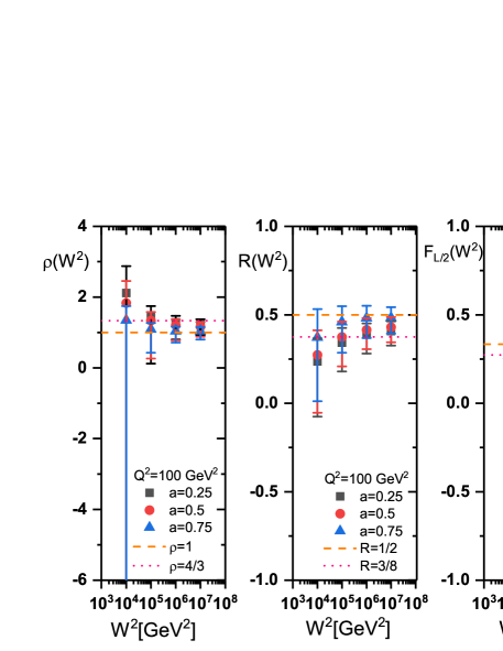
Figure 1: Results of the parameters $\rho,R$ and $F_{L/2}$ obtained from the three expansion points $a=0.25,50$ and $0.75$ respectively. The parameters compared with the CDM bounds $\rho=1$ and $4/3$, $R=1/2$ and $3/8$ and $F_{L/2}=1/3$ and $3/11$ respectively. The results are presented at fixed $Q^{2}$ value in the interval $10^{3}\mathrm{GeV}^{2}<W^{2}<10^{8}\mathrm{GeV}^{2}$ at low values of $x$. The error bars are correspondent to the uncertainties of the $F_{2}$ parameterization (i.e., Table I).

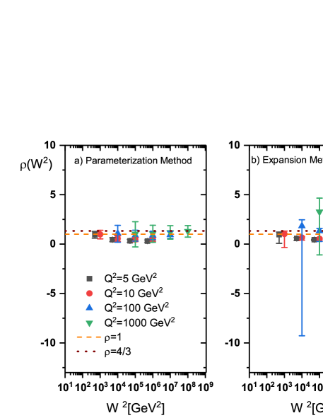
Figure 2: Comparison between the results obtained in parameterization method and expansion method at $a=0.5$ for the $\rho$ parameter. The obtained values compared with the CDM bounds $\rho=1$ and $4/3$. The results are presented at four fixed values of $Q^{2}$ ($Q^{2}=5,~{}10,~{}100~{}\mathrm{and}~{}1000~{}\mathrm{GeV}^{2}$) in the interval $10^{2}\mathrm{GeV}^{2}<W^{2}<10^{8}\mathrm{GeV}^{2}$. The error bars are correspondent to the uncertainties of the $F_{2}$ parameterization (i.e., Table I).

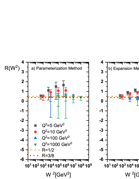
Figure 3: The same as Fig.2 for the ratio $R$ which compared with the CDM bounds $R=1/2$ and $3/8$.

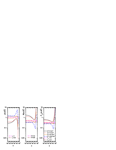
Figure 5: Parameters $\rho$, $R$ and $F_{L/2}$ at LO approximation as a function of $x$ for $Q^{2}=5,~{}10,~{}100$ and $1000~{}\mathrm{GeV}^{2}$ compared with the CDM bounds.

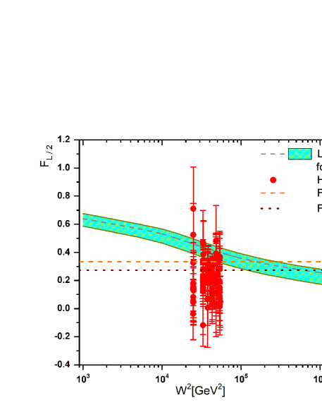
Figure 6: The ratio of the longitudinal to transversal structure functions calculated within the LO approximation at fixed value of the Bjorken variable $x=0.001$. Experimental data are from the H1-Collaboration as accompanied with total errors, Ref.[65] corresponding to the chosen kinematics lies in the interval $1.5~{}\mathrm{GeV}^{2}{\leq}Q^{2}{\leq}150~{}\mathrm{GeV}^{2}$. The obtained values compared with the CDM bounds $F_{L/2}=1/3$ and $3/11$. The error bars are correspondent to the uncertainties of the $F_{2}$ and $F_{L}^{LO}$ parameterization (i.e., Table I and Appendix C).

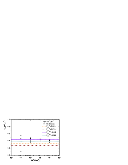
Figure 7: Ratios $F_{L/2}$ plotted as function of the invariant mass $W^{2}$. Straight lines correspond to the CDM bounds at LO and NLO approximations. The obtained values at NLO approximation compared with the NLO CDM bounds $F_{L/2}=0.392$ and $0.442$ [67]. The error bars are correspondent to the uncertainties of the $F_{2}$ and $F_{L}^{NLO}$ parameterization (i.e., Table I and Appendix C).

QCD evolution effects are taken into account by evolving the gluon structure function due to the DGLAP evolution and the Altarelli-Martinelli equation. In the color dipole model the gluon distribution is modified with respect to the parameterization of structure functions at LO and NLO approximations. The ratio of the longitudinal to the transverse photoabsorption cross sections, $\sigma^{\gamma^{*}p}_{L}/\sigma^{\gamma^{*}p}_{T}$, is extracted. This result corresponds to the explicit form of the ratio $F_{2}(x,Q^{2})/G(x,Q^{2})$ by the expansion and Laplace transform methods. The parameters $\rho$, $R$ and $F_{L/2}$ are obtained with respect to the the expansion method at LO approximation and extended to the NLO approximation due to the Laplace transform method. The results obtained in the Laplace transform method at LO and NLO approximations are dependent on the parameterization of the structure functions (i.e., $F_{2}$ and $F_{L}$). These parameterizations [15,21] are valid at low $x$ in a wide range of the momentum transfer $1<Q^{2}<3000\mathrm{GeV}^{2}$. The active flavor is selected in these calculations to be equal to $n_{f}=4$ and the QCD parameter $\Lambda$ has been extracted from the running coupling constant $\alpha_{s}(Q^{2})$ normalized at the Z-boson mass, as it is chosen [63] to be $\alpha_{s}(M_{Z}^{2})=0.1166$ from the ZEUS data [64].
In Fig.1, the parameters $\rho$, $R$ and $F_{L/2}$ are shown in terms of the invariant mass $W^{2}(\simeq\frac{Q^{2}}{x})$ in the interval $10^{3}\mathrm{GeV}^{2}<W^{2}<10^{8}\mathrm{GeV}^{2}$ for three expansion points $a=0.25,0.50$ and $0.75$. In traditional literature, the expansion point of the gluon distribution is chosen by $a=0.50$. Indeed this is the proton momentum fraction carried by gluon in DIS process. In these calculations I used the expansion of the gluon distribution at some arbitrary points and compared with the CDM bounds.
Parameters are almost dependent on the invariant mass in the small expansion points. At high expansion points, the behavior of these parameters is almost independent of the invariant mass, that corresponds to the expansion at $a=0.75$. Also a detailed comparison with the CDM bounds has been shown in this figure (i.e., Fig.1). As can be seen, the values of these parameters are in good agreement with the CDM bounds in a wide range of the invariant mass at fixed value of $Q^{2}$. The error bares are in accordance with the statistical errors of the parameterization of $F_{2}$ as presented in Table I.
An explicit expression for the gluon density into the proton structure function at LO approximation by using the Laplace transform method is derived in Refs.[40]. The result is comparable to the CTEQ5L [65] and MRST2001LO [66], though there are some differences with CTEQ5L for large $x$ values. With respect to this method, a comparison of the parameterization method with expansion method can be seen for the parameters (i.e., $\rho$, $R$ and $F_{L/2}$) in Figs.2-4. In the parameterization method, the gluon obtained by authors in Ref.[41] is used directly. In the expansion method we use the same $a=0.5$ value used in the literature for comparison. As can be seen, the invariant mass dependence in high $Q^{2}$ values is much lower than in low $Q^{2}$ values. According to the range of errors, it can be seen in these figures that the results are in the CDM bounds range. Also, the results of parameterization method are better than expansion method.
Now I proceed with an analysis of the gluon distribution into the parameterization of the structure functions as this is of interests in connection with theoretical investigations of ultra-high energy processes with cosmic neutrinos. Also this method is in the context of the Froissart restrictions at low values of $x$. The longitudinal structure function at low and mediate $x$ values is written in flavour-singlet quark and gluon distributions. Therefore in a new method using the Laplace transform method, the gluon distribution function is expressed in terms of the structure functions at LO and NLO approximations. The method relies on the Altarelli-Martinelli equation and on the Froissart-bounded parameterization of the structure functions.
In Fig.(5) we present the parameters $\rho$, $R=1/(2\rho)$ and $F_{L/2}=1/(1+2\rho)$ at LO approximation related to Eq.(46) in comparison with the CDM bounds using the parameterizations of $F_{2}$ and $F_{L}^{LO}$ [15,21]. As can be seen in this figure, one can conclude that the behavior of these parameters are almost constant and comparable with the CDM bounds at high $Q^{2}$ values for $x\leq 0.01$. Results calculated in LO approximation show that this good comparable is only between the bounds and results for $100{\leq}Q^{2}{\leq}1000~{}\mathrm{GeV}^{2}$. These results show that the parameters are almost $x$ independent for low $x$ values. But they are dependent on $Q^{2}$ values. However this behavior is consistent with the experimental data. However, I need to emphasize that such results are possible only in a limited kinematics, when virtuality $Q^{2}$ is very large and significantly exceeds the saturation scale $Q^{2}_{s}$. These results indicate that the relationship between gluon PDFs and the dipole cross-section is consistent with the CDM bound at high $Q^{2}$ values in order to rewrite the well-known Altarelli-Martinelli relationship for the color dipole framework.
A very important point that can be seen in all the figures (i.e., Figs.1-5) is that the comparability of CDM bounds and results for large $Q^{2}$ values in these calculations takes place in the color transparency region where $\eta{\gg}1$. We observe that for $Q^{2}=5$ and $10~{}\mathrm{GeV}^{2}$ we are practically in the saturation region where $\eta{\ll}1$, which is why the results are inconsistent with CDM bounds. Figure 6 can be seen to express the two concepts of saturation and color transparency in the results. In this figure (i.e., Fig.6) a comparison between the ratio of structure functions at LO approximation with the H1 data [67] and the CDM bounds is shown. For $W^{2}{\gtrsim}10^{4}~{}\mathrm{GeV}^{2}$, the comparison between the ratio $F_{L/2}$ and the H1 data with the bounds is good. This depends on $Q^{2}{\gg}\Lambda^{2}_{sat}(W^{2})$. For $Q^{2}{\ll}\Lambda^{2}_{sat}(W^{2})$ in the saturation region that compatibility is not appropriate at all. The results in the color transparency depend on strong interference between all possible diagrams. While in the saturation region some diagrams are closed which causes the photoabsorption cross section to be ${\ln}\Lambda^{2}_{sat}(W^{2})$ dependent, actually turns into the soft energy dependence. These behaviors are the result of a general and direct consequence of the color dipole nature of the interaction of the hadronic fluctuations of the photon with the color field in the nucleon. Indeed the parameters obtained in the region $\eta{\gg}1$ can give us good results that can be seen in all figures. In terms of the nonlinear behavior of the gluon distribution function, the transition from the region of the validity of pQCD improves parton model at $\eta{\gg}1$ to the saturation region of $\eta{\ll}1$ corresponds to a transition from linear to nonlinear parton distributions. It should be note that the importance of the saturation regime is when the dipole size $r$ is significantly larger, $r\sim 1/Q_{s}$. In other words, the formulas mentioned in this article cannot be used in the saturation regime. For this reason all discussions and final conclusions apply to the color transparency region.
The validity of the results obtained in the LO approximation is established in the $\eta>1$ region. Now the CDM parameters are determined and considered in this region at NLO approximation with respect to the gluon density in Eq.(53). Results of calculations of the ratio $F_{L/2}(W^{2})=\frac{F_{L}(W^{2},Q^{2})}{F_{2}(W^{2},Q^{2})}=\frac{1}{1+2\rho}$ and comparison with the CDM bounds at LO and NLO approximations are presented in Fig.7. Calculations have been performed at fixed value $Q^{2}=100~{}\mathrm{GeV}^{2}$ at low values of $x$, allowing the invariant mass variable $W^{2}$ to vary in the interval $10^{3}\mathrm{GeV}^{2}<W^{2}<10^{8}\mathrm{GeV}^{2}$. Figure 7 clearly demonstrates that the ratio extracted is comparable with the NLO CDM bound. In fact, I have shown that Eq.(22), which represents the relation between the gluon density and CDM bounds in the color transparency region, can also be described at NLO approximation. In conclusion this method defined consistency between the CDM bounds and gluon PDFs in the color transparency region.

.9 5. Conclusion

In this paper the CDM parameters (i.e., $\rho$, $R$ and $F_{L/2}$) based on one general expression for approximative determination of the gluon distribution for very small dipoles presented. The gluon behavior at arbitrary point of expansion of $G(\frac{x}{1-z})$ is considered. Comparing the obtained results with the CDM bounds, it can be concluded that the more suitable points of expansion are in the range $a\geq 0.75$. Then a method based on the Altarelli-Martinelli equation and on the Froissart-bounded parameterization of $F_{2}$ and $F_{L}$ with respect to the Laplace transform method at LO and NLO approximations when virtuality $Q^{2}$ is large is proposed. The parameters obtained on the kinematic region of low and ultra-low values of $x$ in a large interval of the momentum transfer at LO approximation. At NLO approximation we focus our attention on value $Q^{2}=100~{}\mathrm{GeV}^{2}$. The obtained explicit expressions for the parameters are entirely determined by the effective parameters of the $F_{2}$ and $F_{L}$ parameterizations. The results obtained for the ratio $F_{L/2}$ at NLO approximation in the color transparency region are in good agreement with the NLO CDM bound which have considered the contribution of the $q\overline{q}g$ component in the the colored sector of the virtual photon wave-function.
According to the relationships obtained in the color transparency region at large $Q^{2}$ values, we observe that the results obtained are comparable to the H1 data and the CDM bounds. These results indicate that for $Q^{2}{\gg}\Lambda^{2}_{sat}(W^{2})$ the relationships obtained on the basis of the parameterization of $F_{2}$ and $F_{L}$ are comparable to the proposed constraints. The predictions are most reliable for $20\mathrm{GeV}^{2}{\leq}Q^{2}\leq 1000\mathrm{GeV}^{2}$ at $x{\leq}0.01$. The behavior of the parameters is independent of $x$ for large $Q^{2}$ values and are almost dependent on $Q^{2}$ in a wide range of $Q^{2}$ values. They become less reliable, when $Q^{2}$ decreases to $Q^{2}<20\mathrm{GeV}^{2}$, since in this case the transition to the saturation region has to be refined by the nonlinear effects. Indeed in the saturation region the dipole size $r$ is significantly large which causes neither DGLAP evolution nor the formulas listed in this paper to be used in the saturated regime.

.10 ACKNOWLEDGMENTS

Author is grateful the Razi University for financial support of this project. The author is especially grateful to N.Nikolaev and D.Schildknecht for carefully reading the manuscript and fruitful discussions.

.11 Appendix A. Details on the Derivation of (26)

In this Appendix, I provide a brief exposition of the derivation Eq.(26) in Ref.[34]. The evolution equations for the parton distributions are defined by

$$\frac{\partial}{\partial{\ln}Q^{2}}f_{i}(x,Q^{2})=P_{ij}(x,Q^{2}){\otimes}f_{j}(x,Q^{2}),$$ (57)

where $f_{i}(x,Q^{2})$ stands for the number distributions of partons in a hadron and $\otimes$ stands for the Mellin convolution. This equation (i.e., Eq.(57)) represents a system of $2n_{f}+1$ coupled integro-differential equations. The splitting functions $P_{ij}(x,Q^{2})$ for $N^{m}LO$ approximation are defined by $P^{N^{m}LO}_{ij}(x,Q^{2})=\sum_{k=0}^{m}a_{s}^{k+1}(Q^{2})P_{ij}^{k}(x)$ with $a_{s}(Q^{2})=\alpha_{s}(Q^{2})/4\pi$. The flavor singlet quark density is defined $f_{s}=\sum_{i=1}^{n_{f}}[f_{i}+\overline{f}_{i}]$. The LO evolution equation for $F_{2}$ at low $x$ for four flavors is defined by

$$\frac{\partial F_{2}(x,Q^{2})}{\partial{\ln}Q^{2}}=\frac{10\alpha_{s}}{9\pi}\int_{0}^{1-x}P_{qg}(z)G(\frac{x}{1-z},Q^{2})dz.$$ (58)

Here the fact is used that at low values of $x$ quark density can be neglected and the nonsinglet contribution can be ignored. The authors [34] used the expansion of the gluon distribution at an arbitrary point $z=a$ as at the limit $x{\rightarrow}0$, the equation obtained is

$$\frac{\partial F_{2}(x,Q^{2})}{\partial{\ln{Q^{2}}}}\simeq\frac{5\alpha_{s}(Q^{2})}{9\pi}\frac{2}{3}G(\frac{x}{1-a}(\frac{3}{2}-a),Q^{2}).$$ (59)

Therefore the gluon distribution can be expressed by

$$G(x,Q^{2})=\frac{9\pi}{5\alpha_{s}(Q^{2})}\frac{3}{2}\frac{\partial F_{2}(x\frac{1-a}{\frac{3}{2}-a},Q^{2})}{\partial{\ln{Q^{2}}}}.$$ (60)

The result of comparing them with GRV94(LO) [42] showed that the better choices have been in the range $0.5{\leq}a{\leq}0.8$ and with Ryskin $et~{}al.$ [43] corresponds to $a=0.75$.

.12 Appendix B: Details on the Derivation of (32)

The gluon density used in this analysis obeys the following Laplace-transform method [44-53], as the coordinate transformation introduced by $\upsilon{\equiv}{\ln}(1/x)$. Further, Eq.(31) rewritten by the following form

$$\widehat{\mathcal{F}}(\upsilon,Q^{2})=\int_{0}^{\upsilon}\widehat{G}(w,Q^{2})\widehat{H}(\upsilon-w){dw},$$ (61)

where $\widehat{H}(\upsilon){\equiv}e^{-\upsilon}\widehat{K}_{qg}(\upsilon)$ and $\widehat{f}(\upsilon,Q^{2}){\equiv}f(e^{-\upsilon},Q^{2})$ as $\widehat{K}_{qg}(\upsilon)=1-2e^{-\upsilon}+2e^{-2\upsilon}$. The Laplace transform of the right-hand of Eq.(61) is defined by

$$\mathcal{L}\bigg{[}\int_{0}^{\upsilon}\widehat{G}(w,Q^{2})\widehat{H}(\upsilon-w){dw};s\bigg{]}=g(s){\times}h(s)$$ (62)

where $h(s){\equiv}\mathcal{L}[\widehat{H}(\upsilon);s]=\int_{0}^{\infty}\widehat{H}(\upsilon)e^{-s\upsilon}d\upsilon$ with the condition $\widehat{H}(\upsilon)=0$ for $\upsilon<0$.
The gluon distribution function in $\upsilon$-space is obtained in terms of the inverse transform of a product to the convolution of the original functions as

$$\widehat{G}(\upsilon,Q^{2}) = \mathcal{L}^{-1}[f(s,Q^{2}{\times}h^{-1}(s);\upsilon]$$ (63)

$$=\int_{0}^{\upsilon}\widehat{\mathcal{F}}(w,Q^{2})\widehat{J}(\upsilon-w){dw},$$

where

$$\widehat{J}(\upsilon) {\equiv} \mathcal{L}^{-1}[h^{-1}(s);\upsilon]$$ (64)

$$=3\delta(\upsilon)+\delta^{\prime}(\upsilon)-e^{-3\upsilon/2}\big{\{}\frac{6}{\sqrt{7}}\sin[\frac{\sqrt{7}}{2}\upsilon]$$

$$+2\cos[\frac{\sqrt{7}}{2}\upsilon]\big{\}}.$$

Therefore the explicit solution for the gluon distribution in $\upsilon$-space is defined in terms of the integral

$$\widehat{G}(\upsilon,Q^{2}) = 3\widehat{\mathcal{F}}(\upsilon,Q^{2})+\frac{\partial\widehat{\mathcal{F}}(\upsilon,Q^{2})}{\partial{\upsilon}}-\int_{0}^{\upsilon}\widehat{\mathcal{F}}(w,Q^{2})$$ (65)

$${\times}e^{-3(\upsilon-w)/2}\big{\{}\frac{6}{\sqrt{7}}\sin[\frac{\sqrt{7}}{2}(\upsilon-w)]$$

$$+2\cos[\frac{\sqrt{7}}{2}(\upsilon-w)]\big{\}}.$$

.13 Appendix C: Details about the parameterization of $F_{L}(x,Q^{2})$

The authors in Ref.[21] obtained two analytical relations for the longitudinal structure function at LO and NLO approximations in terms of the effective parameters of the parameterization of the proton structure function. The results show that the obtained method provides reliable longitudinal structure function at HERA domain and also the structure functions $F_{L}(x,Q^{2})$ manifestly obey the Froissart boundary conditions. The structure functions, $F_{2}(x,Q^{2})$ and $F_{L}(x,Q^{2})$, and their derivatives into $\ln Q^{2}$ are defined with respect to the singlet and gluon distribution functions $xf_{a}(x,Q^{2})$ as

$$F_{k\{=2,L\}}(x,Q^{2}) = <e^{2}>\sum_{a=s,g}[B_{k,a}(x){\otimes}xf_{a}(x,Q^{2})]$$

$$\mathrm{and}~{}~{}~{}~{}~{}~{}~{}~{}~{}~{}~{}~{}~{}~{}~{}$$

$$\frac{\partial}{\partial{\ln}Q^{2}}xf_{a}(x,Q^{2}) = -\frac{1}{2}\sum_{a,b=s,g}P_{ab}(x){\otimes}xf_{b}(x,Q^{2}).$$ (66)

The quantities $B_{k,a}(x)$ and $P_{ab}(x)$ are the Wilson coefficient and splitting functions respectively. The high order corrections to the coefficient functions can be seen in Ref.[21]. With respect to the Mellin transform method, the leading order longitudinal structure function is obtained at low $x$ by the following form

$$F_{L}^{\mathrm{LO}}(x,Q^{2}) = (1-x)^{n}\sum_{m=0}^{2}C_{m}(Q^{2})L^{m},$$ (67)

where

$$C_{2} = \widehat{A}_{2}+\frac{8}{3}a_{s}(Q^{2})DA_{2}$$

$$C_{1} = \widehat{A}_{1}+\frac{1}{2}\widehat{A}_{2}+\frac{8}{3}a_{s}(Q^{2})D[A_{1}+(4\zeta_{2}-\frac{7}{2})A_{2}]$$

$$C_{0} = \widehat{A}_{0}+\frac{1}{4}\widehat{A}_{2}-\frac{7}{8}\widehat{A}_{2}+\frac{8}{3}a_{s}(Q^{2})D[A_{0}+(2\zeta_{2}-\frac{7}{4})A_{1}$$ (68)

$$+(\zeta_{2}-4\zeta_{3}-\frac{17}{8})A_{2}],$$

and

$$\widehat{A}_{2} = \widetilde{A}_{2}$$

$$\widehat{A}_{1} = \widetilde{A}_{1}+2DA_{2}\frac{\mu^{2}}{\mu^{2}+Q^{2}}$$

$$\widehat{A}_{0} = \widetilde{A}_{0}+DA_{1}\frac{\mu^{2}}{\mu^{2}+Q^{2}}$$

$$\widetilde{A}_{i} = \widetilde{D}A_{i}+D\overline{A}_{i}\frac{Q^{2}}{Q^{2}+\mu^{2}}$$

$$\widetilde{D} = \frac{M^{2}Q^{2}[(2-\lambda)Q^{2}+\lambda M^{2}]}{[Q^{2}+M^{2}]^{3}}$$

$$\overline{A}_{m} = a_{m1}+2a_{m2}L_{2},~{}~{}a_{02}=0.$$ (69)

The standard representation for QCD running coupling constant in the LO and NLO approximations have been described

$$a_{s}^{\mathrm{LO}}(Q^{2}) = \frac{1}{\beta_{0}\ln(Q^{2}/\Lambda^{2})},$$ (70)

$$a_{s}^{\mathrm{NLO}}(Q^{2}) = \frac{1}{\beta_{0}\ln(Q^{2}/\Lambda^{2})}-\frac{\beta_{1}{\ln}\ln(Q^{2}/\Lambda^{2})}{\beta_{0}[\beta_{0}\ln(Q^{2}/\Lambda^{2})]^{2}},$$

which the QCD parameter $\Lambda$ at LO and NLO approximations has been extracted with $\Lambda^{LO}(n_{f}=4)=136.8~{}\mathrm{MeV}$ and $\Lambda^{NLO}(n_{f}=4)=284.0~{}\mathrm{MeV}$ respectively. The QCD $\beta$-functions are

$$\beta_{0}=\frac{1}{3}(11C_{A}-2n_{f}),~{}\beta_{1}=\frac{1}{3}(34C_{A}^{2}-2n_{f}(5C_{A}+3C_{F}))$$

where $C_{F}$ and $C_{A}$ are the Casimir operators in the $SU(N_{c})$ color group.
The NLO longitudinal structure function at small $x$ is defined by the following form

$$F_{L}^{\mathrm{NLO}}(x,Q^{2}) = \frac{1}{[1+\frac{1}{3}a_{s}(Q^{2})L_{C}(\widehat{\delta}^{(1)}_{sg}-\widehat{R}^{(1)}_{L,g})]}\bigg{\{}$$

$$[1-a_{s}(Q^{2})(\overline{\delta}^{(1)}_{sg}-\overline{R}^{(1)}_{L,g})]F_{L}^{\mathrm{LO}}(x,Q^{2})$$

$$-a^{2}_{s}(Q^{2})[\frac{1}{3}\widehat{B}^{(1)}_{L,s}L_{A}+\overline{B}^{(1)}_{L,s}]F_{2}(x,Q^{2})\bigg{\}}$$

where the coefficient functions read as

$$\widehat{B}^{(1)}_{L,s} = 8C_{F}[\frac{25}{9}n_{f}-\frac{449}{72}C_{F}+(2C_{F}-C_{A})$$

$$(\zeta_{3}+2\zeta_{2}-\frac{59}{72})]$$

$$\overline{B}^{(1)}_{L,s} = \frac{20}{3}C_{F}(3C_{A}-2n_{f})$$

$$\widehat{\delta}^{(1)}_{sg} = \frac{26}{3}C_{A}$$

$$\overline{\delta}^{(1)}_{sg} = 3C_{F}-\frac{347}{18}C_{A}$$

$$\widehat{R}^{(1)}_{L,g} = -\frac{4}{3}C_{A}$$

$$\overline{R}^{(1)}_{L,g} = -5C_{F}-\frac{4}{9}C_{A}$$

$$L_{A} = L+\frac{A_{1}}{2A_{2}}$$

$$L_{C} = L+\frac{C_{1}}{2C_{2}}$$

$$L = \ln(1/x)+L_{1}$$

$$L_{1} = {\ln}\frac{Q^{2}}{Q^{2}+\mu^{2}}.$$ (72)

Table 1: The effective Parameters at low $x$ for $0.15~{}\mathrm{GeV}^{2}<Q^{2}<3000~{}\mathrm{GeV}^{2}$ provided by the following values. The fixed parameters are defined by the Block-Halzen fit [39] to the real photon-proton cross section as $M^{2}=0.753\pm 0.068~{}\mathrm{GeV}^{2}$ and $\mu^{2}=2.82\pm 0.290~{}\mathrm{GeV}^{2}$.

parameters                    value
$a_{00}$	$2.550\times 10^{-1}~{}\pm 1.60\times 10^{-2}$
$a_{01}$	$1.475\times 10^{-1}~{}\pm 3.025\times 10^{-2}$
$a_{10}$	$8.205\times 10^{-4}~{}~{}\pm 4.62\times 10^{-4}$
$a_{11}$	$-5.148\times 10^{-2}\pm 8.19\times 10^{-3}$
$a_{12}$	$-4.725\times 10^{-3}\pm 1.01\times 10^{-3}$
$a_{20}$	$2.217\times 10^{-3}\pm 1.42\times 10^{-4}$
$a_{21}$	$1.244\times 10^{-2}\pm 8.56\times 10^{-4}$
$a_{22}$	$5.958\times 10^{-4}\pm 2.32\times 10^{-4}$
$n$	$11.49\pm 0.99$
$\lambda$	$2.430~{}\pm 0.153$
$\chi^{2}(\mathrm{goodness~{}of~{}fit})$	$0.95$

I References

1. N.N.Nikolaev and B.G.Zakharov, Z.Phys.C49, 607(1991); N.N.Nikolaev and B.G.Zakharov, Z.Phys.C53, 331(1992); A.H.Mueller, Nucl.Phys.B415, 373(1994); Nucl.Phys.B437, 107(1995); K.Golec-Biernat, Acta Phys.Pol.B35, 3103(2004).
2. R.J.Glauber, Phys.Rev.99, 1515(1955); A.H.Mueller, Nucl.Phys.B335, 115(1990).
3. K.Golec-Biernat and M.W$\mathrm{\ddot{u}}$sthoff, Phys.Rev.D59, 014017(1998); K.Golec-Biernat and M.W$\mathrm{\ddot{u}}$sthoff, Phys.Rev.D60, 114023(1999).
4. K.Golec-Biernat, Acta Phys.Pol.B33, 2771(2002); J.Phys.G28, 1057(2002); H.Kowalski and D.Teaney, Phys.Rev.D68, 114005(2003); H.Kowalski, L.Motyka and G.Watt, Phys.Rev.D74, 074016(2006).
5. C.Ewerz, A.von Manteuffel and O.Nachtmann, JHEP03, 102(2010); D.Britzger et al., Phys.Rev.D100, 114007 (2019); C.Ewerz, A. von Manteuffel and O.Nachtmann, Phys.Rev.D77, 074022(2008).
6. H.Kowalski and D.Teaney, Phys.Rev.D68, 114005(2003).
7. G.Watt and H.Kowalski, Phys.Rev.D78, 014016(2008); A.H.Rezaeian et al., Phys.Rev.D87, 034002(2013).
8. L.McLerran, arXiv:0804.1736 [hep-ph] (2008); Acta.Phys.Polon.B45, 2307 (2014).
9. F. Gelis et al., Annu. Rev. Nucl. Part. Sci. 60, 463 (2010); G.M.Peccini et al., Phys. Rev. D101, 074042 (2020); M.Genovese, N.N.Nikolaev and B.G.Zakharov, J.Exp.Theor.Phys.81, 633(1995); J.Exp.Theor.Phys.81, 625(1995); Amir H.Rezaeian and I.Schmidt, Phys.Rev. D88, 074016 (2013).
10. I.Balitsky, Nucl.Phys.B463, 99(1996); Phys.Rev.D75, 014001(2007); Y.V.Kovchegov, Phys.Rev.D60, 034008(1999); Phys.Rev.D61, 074018(2000).
11. E.Iancu,K.Itakura and S.Munier, Phys.Lett.B590, 199(2004).
12. A.M.Stasto, K.Golec-Biernat, J.Kwiecinski, Phys.Rev.Lett.86, 596(2001); F.Gelis et al., Phys.Lett.B647, 376(2007); J.Kwiecinski and A.M.Stasto, Phys.Rev.D66, 014013(2002).
13. D.Schildknecht and H.Spiesberger, arXiv [hep-ph]: 9707447 (1997); W.Buchmuller and D.Haidt, arXiv [hep-ph]: 9605428 (1996) .
14. M.Froissart, Phys.Rev.123, 1053(1961).
15. M. M. Block, L. Durand and P. Ha, Phys. Rev.D89, no. 9, 094027 (2014); M.M.Block et al., Phys. Rev.D88, no. 1, 014006 (2013).
16. D.Boer et al., arXiv: [nucl-th]1108.1713.
17. M.Klein, arXiv [hep-ph]:1802.04317; M.Klein, Ann.Phys.528, 138(2016); N.Armesto et al., Phys.Rev.D100, 074022(2019).
18. J.Abelleira Fernandez et al., [LHeC Study Group Collaboration], J.Phys.G39, 075001(2012).
19. P.Agostini et al. [LHeC Collaboration and FCC-he Study Group ], CERN-ACC-Note-2020-0002, arXiv:2007.14491 [hep-ex] (2020).
20. A. Abada et al., [FCC Study Group Collaboration], Eur.Phys.J.C79, 474(2019).
21. L.P.Kaptari et al., Phys.Rev.D99, 096019 (2019).
22. B.Rezaei and G.R.Boroun, Phys.Rev.C101, 045202 (2020).
23. G.R.Boroun and B.Rezaei, Nucl.Phys.A990, 244(2019).
24 K.Golec-Biernat and S.Sapeta, JHEP 03, 102 (2018); J.Bartels, K.Golec-Biernat and H.Kowalski, Phys.Rev.D66, 014001(2002).
25. G.Beuf, Phys.Rev.D94, 054016(2016); Phys.Rev.D96, 074033 (2017); G.Beuf et al., arXiv:2008.05233[hep-ph] (2020).
26. B.Duclou$\mathrm{\acute{e}}$ et al., Phys.Rev.D96, 094017(2017); J.Bartels et al., Phys.Rev.D81, 054017(2010).
27. N.N.Nikolaev and B.G.Zakharov, Phys.Lett.B333, 250(1994); L.Frankfurt, A.Radyushkin and M.Strikman, Phys.Rev.D55, 98(1997); M. Genovese, N.N. Nikolaev and B.G. Zakharov, JETP 81, 633(1995); I.P. Ivanov and N.N. Nikolaev, Phys. Rev. D 65, 054004 (2002).
28. M.Kuroda and D.Schildknecht, Phys.Lett. B618, 84(2005); M.Kuroda and D.Schildknecht, Acta Phys.Polon. B37, 835(2006); M.Kuroda and D.Schildknecht, Phys.Lett. B670, 129(2008); M.Kuroda and D.Schildknecht, Phys.Rev. D96, 094013(2017).
29. D.Schildknecht and M.Tentyukov, arXiv[hep-ph]:0203028; M.Kuroda and D.Schildknecht, Phys.Rev. D85, 094001(2012); D.Schildknecht, Mod.Phys.Lett.A29, 1430028(2014); M.Kuroda and D.Schildknecht, Int. J. Mod. Phys. A31, 1650157 (2016).
30. M.Kuroda and D.Schildknecht, Phys.Rev.D31, 094001(2014).
31. D.Schildknecht, B.Surrow and M.Tentynkov, Phys.Lett.B499, 116(2001); G.Cvetic , D.Schildknecht, B.Surrow and M.Tentynkov, Eur.Phys.J.C20, 77(2001); D.Schildknecht, B.Surrow and M.Tentynkov, Mod.Phys.Lett.A16, 1829(2001); M.Kuroda and D.Schildknecht, Eur.Phys.J.C37, 205(2004).
32. K.Prytz, Phys.lett.B311, 286(1993).
33. A.M.Cooper-Sarkar et al., Z.Phys.C39, 281(1988); A.M.Cooper-Sarkar et al., Acta Phys.Pol.B34, 2911(2003).
34. M.B.Gay Ducati and Victor P.B.Goncalves, Phys.Lett.B390, 401(1997).
35. G.R.Boroun and B.Rezaei, Eur.Phys.J.C72, 2221(2012).
36. B.Rezaei and G.R.Boroun, Eur.Phys.J.A56, 262 (2020).
37. G.R.Boroun and B.Rezaei, Phys.Lett.B 816, 136274 (2021).
38. F.D.Aaron et al., [H1 and ZEUS Collaborations], JHEP1001, 109(2010).
39. M.M.Block and F.Halzen, Phys.Rev.Lett.107, 212002 (2011); Phys.Rev.D70, 091901 (2004).
40. Yu.L.Dokshitzer, Sov.Phys.JETP 46, 641(1977); G.Altarelli and G.Parisi, Nucl.Phys.B 126, 298(1977); V.N.Gribov and L.N.Lipatov, Sov.J.Nucl.Phys. 15, 438(1972).
41. Martin M.Block, Eur.Phys.J.C65, 1 (2010); M. M. Block, L. Durand and Douglas W.McKay, Phys. Rev.D79, 0140131 (2009); Phys. Rev.D77, 094003 (2008).
42. M.Gluk, E.Reya and A.Vogt, Z.Phys.C67, 433(1995).
43. M.G.Ryskin, Yu. M.Shabelski and A.G.Shuvaev, Z.Phys.C73, 111(1996).
44. M.M.Block, L.Durand and D.W.McKay, Phys.Rev.D79, 014031(2009); M.M.Block, Eur.Phys.J.C65, 1(2010).
45. F.Taghavi-Shahri, A.Mirjalili and M.M.Yazdanpanah, Eur.Phys.J.C71, 1590(2011).
46. S.M.Moosavi Nejad et al., Phys.Rev.C94, 045201(2016).
47. H.Khanpour, A.Mirjalili and S.Atashbar Tehrani, Phys.Rev.C95, 035201(2017).
48. G.R. Boroun, S. Zarrin and F. Teimoury, Eur.Phys.J.Plus130, 214(2015).
49. G.R. Boroun and S. Zarrin, Phys.Atom.Nucl.78, 1034(2015).
50. G.R. Boroun, S. Zarrin and S. Dadfar, Nucl.Phys.A953, 21(2016).
51. G.R. Boroun, S. Zarrin and S. Dadfar, Phys.Atom.Nucl.79, 236(2016).
52. F. Teimoury Azadbakht, G.R. Boroun and B. Rezaei, Int.J.Mod.Phys.E27, 1850071(2018).
53. S.Dadfar and S.Zarrin, Eur.Phys.J.C80, 319(2020).
54. S.Moch, J.A.M.Vermaseren and A.Vogt, Phys.Lett.B606, 123(2005); D.I.Kazakov et al., Phys.Rev.Lett.65, 1535(1990).
55. G.Altarelli and G.Martinelli, Phys.Lett.B76, 89(1978).
56. N.Baruah, M.K.Das and J.K.Sarma, Few-Body Syst.55, 1061(2014); N.Baruah, N.M.Nath and J.K.Sarma, Int.J.Theor.Phys.52, 2464(2013).
57. G.R.Boroun, Phys.Rev.C97, 015206(2018).
58. G.R.Boroun, Int.J.Mod.Phys.E18, 131(2009).
59. G.R.Boroun, B.Rezaei and J.K.Sarma, Int.J.Mod.Phys.A29, 1450189(2014).
60. G.R.Boroun, Eur.Phys.J.Plus129, 19(2014).
61. G.Beuf, Phys. Rev. D 85, 034039(2012).
62. M.Niedziela and M.Praszalowicz, Acta Physica Polonica B46, 2018(2015).
63. K.G.Chetyrkin, B.A.Kniehl and M.Steinhauser, Phys.Rev.Lett.79, 2184(1997); Nucl.Phys.B510, 61(1998).
64. S.Chekanov et al.[ZEUS Collaboration], Eur.Phys.J.C21,443(2001).
65. H.L.Lai et.al. [CTEQ Collaboration], Eur.Phys.J.C12, 375(2000).
66. A.D.Martin, R.G.Roberts, W.J.Stirling and R.S.Thorne, MRST2001, Eur.Phys.J.C23, 73(2002).
67. V.Andreev et al. [H1 Collaboration], Eur.Phys.J.C74, 2814(2014).

Figure 4: The same as Fig.2 for the ratio $F_{L/2}$ which compared with the CDM bounds $F_{L/2}=1/3$ and $3/11$.