Duffing-type equations: singular points of amplitude profiles and bifurcations

Abstract

We study the Duffing equation and its generalizations with polynomial nonlinearities. Recently, we have demonstrated that metamorphoses of the amplitude response curves, computed by asymptotic methods in implicit form as $F\left(\Omega,\ A\right)=0$, permit prediction of qualitative changes of dynamics occurring at singular points of the implicit curve $F\left(\Omega,\ A\right)=0$. In the present work we determine a global structure of singular points of the amplitude profiles computing bifurcation sets, i.e. sets containing all points in the parameter space for which the amplitude profile has a singular point. We connect our work with independent research on tangential points on amplitude profiles, associated with jump phenomena, characteristic for the Duffing equation. We also show that our techniques can be applied to solutions of form $\Omega_{\pm}=f_{\pm}\left(A\right)$, obtained within other asymptotic approaches.

1 Introduction

Recently, nonlinear Duffing-type oscillators attracted considerable attention due to a rich variety of engineering applications. A very interesting class of generalized Duffing oscillators with polynomial nonlinearities is described by the following equation:

$$m\frac{d^{2}x}{dt^{2}}+\mu\frac{dx}{dt}+k_{1}x+k_{3}x^{3}+k_{5}x^{5}+\ldots+k_{n}x^{n}=a\cos\left(\omega t\right),$$ (1)

which, for example, can model dynamics of a mathematical pendulum or a ship-roll motions [1, 2, 3, 4, 5, 6, 7, 8, 9, 10]. In (1) $m$ is the mass, $\mu$ is the damping parameter, $k_{1}$ can be interpreted as the linear stiffness coefficient, $k_{n}\ \left(n=3,5,\ldots\right)$ are parameters of the nonlinear restoring force, while $a$, $\omega$ are the amplitude and angular frequency of the periodic driving force, respectively.

Nonlinear reponses of form $x\left(t\right)=A\left(\omega\right)\cos\left(\omega t+\varphi\left(\omega\right)\right)$ can be computed by any of many asymptotic methods [11]. In the present work we compute the asymptotic solutions in implicit form as $F\left(\omega,\ A,\text{\ }\underline{c}\right)=0$, where $\underline{c}=\left(c_{1},c_{2},\ldots,c_{m}\right)$ are parameters, by the application of the Krylov-Bogoliubov-Mitropolsky (KBM) method [11].

As explained in Section 3 and demonstrated in our earlier papers qualitative changes of dynamics occur at singular points of the implicit amplitude equation $F\left(\omega,\ A,\text{\ }\underline{c}\right)=0$ (also known as the  amplitude-frequency response or the amplitude response equation), see [12] and references therein. Singular points appear at some special values of parameters $\underline{c}=\underline{c}_{\ast}$, for which the implicit function $F$ fulfills appropriate equations, see Eqs. (13). In other words, at $\underline{c}=\underline{c}_{\ast}$ there is a change of differential properties of the amplitude response curve $F\left(\omega,\ A,\text{\ }\underline{c}_{\ast}\right)=0$ at a singular point $\left(\omega_{\ast},\ A_{\ast}\right)$, referred to as a metamorphosis.

In this work, we attempt to find a global picture of singular points of the amplitude response equation for the generalized Duffing equation (1). We derive formulae for singular points and the bifurcation set in general case and apply these results to the case of the standard cubic Duffing equation ($n=3$) and to the cubic-quintic Duffing equation ($n=5$). We shall carry out this program for higher values of $n$ in our future work.

In Section 7 we connect our work on singular metamorphoses with research on changes of differential properties of amplitude-frequency response curves in a non-singular case, which can be viewed as non-singular metamorphoses [2]. Metamorphoses described in [2] can be classified as vertical tangencies – for some parameter values the amplitude response curve has vertical tangent points (critical but non-singular) associated with saddle-node bifurcations (jump phenomena) [2].

In A we analyse metamorphoses of the amplitude profiles from another point of view. Implicit equation $F\left(\Omega,\ A\right)=0$ can be solved for $\Omega$ for the generalized Duffing equation so that we can get explicit solutions $\Omega_{\pm}=f_{\pm}\left(A\right)$. Intersection conditions for these two branches, $f_{+}\left(A\right)=f_{-}\left(A\right)$, yield singular points of the amplitude profile (the same as described in Section 4.3, obtained within the more general approach of Section 4.2). We present a more detailed picture of transformation of a non-singular amplitude profile into a self-intersection, non-singular amplitude, and into amplitude with an isolated point.

We also apply our approach to explicit solutions $\omega_{\pm}=g_{\pm}\left(A\right)$ computed in [5] for the cubic-quintic oscillator obtained via the Multiple Scales Linstedt Poincaré (MSLP) method, see B. We show that our techniques, described in Section 4 as well as in the A), can be applied to amplitudes obtained within another asymptotic approach.

Finally, in C computational details are described.

2 The Krylov-Bogoliubov-Mitropolsky amplitude profiles for the generalized Duffing equation

Introducing nondimensional units, $\Omega=\dfrac{\omega}{\omega_{n}}$, $\omega_{n}=\sqrt{\dfrac{k_{1}}{m}}$, $\tau=\omega_{n}t$, Eq. (1) is cast into form:

$$\ddot{y}+h\dot{y}+y+c_{3}y^{3}+c_{5}y^{5}+\ldots+c_{n}y^{n}=f\cos\left(\Omega\tau\right),$$ (2)

where overdots denote derivatives with respect to $\tau$ and $n=3,5,7,9,\ldots$ . We assume that parameters $h$, $c_{3}$, …, $c_{n}$, $f$ are small and can be thus written as $h=\varepsilon\bar{h}$, $c_{3}=\varepsilon\bar{c}_{3}$, …, $c_{n}=\varepsilon\bar{c}_{n}$, $f=\varepsilon\bar{f}$ where $\varepsilon$ is a small parameter and $\bar{h}$, $\bar{c}_{3}$, …, $\bar{c}_{n}$, $\bar{f}$ are of order $O\left(1\right)$.

Looking for $1:1$ resonances we rewrite equation 2 in form of a weakly perturbed system:

$$\frac{d^{2}y}{d\tau^{2}}+\Omega^{2}y+\varepsilon\left(\sigma y+g\right)=0,$$ (3)

where

$$g = \bar{h}\frac{dy}{d\tau}+\bar{c}_{3}y^{3}+\bar{c}_{5}y^{5}+\ldots+\bar{c}_{n}y^{n}-\bar{f}\cos\left(\Omega\tau\right),$$ (4a)

$$\varepsilon\sigma = 1-\Omega^{2},$$ (4b)

and $\sigma=O\left(1\right)$.

We apply the Krylov-Bogoliubov-Mitropolsky (KBM) perturbation approach [11] assuming the $1:1$ resonance in form:

$$y=A\left(\tau\right)\cos\left(\Omega\tau+\varphi\left(\tau\right)\right)+\varepsilon y_{1}\left(A,\varphi,\tau\right)+\ldots$$ (5)

with slowly varying amplitude $A$ and phase $\varphi$:

$$\frac{dA}{d\tau} = \varepsilon M_{1}\left(A,\varphi\right)+\ldots,$$ (6a)

$$\frac{d\varphi}{d\tau} = \varepsilon N_{1}\left(A,\varphi\right)+\ldots,$$ (6b)

obtaining:

$$M_{1} = \frac{1}{2\Omega}\left(-\bar{h}A\Omega-\bar{f}\sin\varphi\right),$$ (7a)

$$N_{1} = \frac{1}{2\Omega A}\left(\sigma A+\bar{d}_{3}A^{3}+\bar{d}_{5}A^{5}+\ldots\bar{d}_{n}-\bar{f}\cos\varphi\right),$$ (7b)

with $\bar{d}_{n}$ given in (9).

The fixed points of the slow-flow equations (6), (7) correspond to solutions with constant amplitude and phase [2]. We thus demand that $M_{1}=N_{1}=0$, eliminate $\varphi$, and get the following implicit amplitude-frequency equation:

$$\begin{array}[]{l}L_{n}\left(X,Y\right)=h^{2}XY+Y\left(X-1-d_{3}Y-d_{5}Y^{2}-\ldots-d_{n}Y^{n}\right)^{2}-f^{2}=0\vskip 3.0pt plus 1.0pt minus 1.0pt\\ X\equiv\Omega^{2},\ Y\equiv A^{2}\end{array}$$ (8)

and

$$\bar{d}_{n}=2^{\frac{1-n}{2}}\frac{n!!}{\left(\frac{n+1}{2}\right)!}\ \bar{c}_{n},\quad n=3,5,7,9,\ldots.$$ (9)

In what follows we shall also write $F\left(\Omega,A\right)=L_{n}\left(\Omega^{2},A^{2}\right)$.

3 Singular points of amplitude profiles and bifurcations of dynamics

Detailed description of properties and applications of singular points of amplitude profiles can be found in Ref. [12]. In short, solving a nonlinear differential equation of form:

$$\frac{d^{2}y}{d\tau^{2}}+\omega^{2}y=\varepsilon f\left(y,\frac{dy}{d\tau},\tau\right),$$ (10)

where $\varepsilon$ is a small parameter and $f$ is a periodic function of time $\tau$ with period $T=\frac{2\pi}{\Omega}$, by an asymptotic method we find an approximate solution:

$$y\left(\tau\right)=A\left(\Omega\right)\cos\left(\Omega\tau+\varphi\left(\Omega\right)\right)+\varepsilon y_{1}\left(\tau\right)+\ldots$$ (11)

where the amplitude $A$ and frequency $\Omega$ fulfill the amplitude response equation:

$$F\left(\Omega,A;\underline{c}\right)=0,$$ (12)

where $\underline{c}=\left(c_{1},c_{2},\ldots,c_{m}\right)$ are parameters. Equation (12) defines an implicit function – a two-dimensional planar curve - the amplitude-frequency response curve (the amplitude profile). The form of this curve, as well as stability of the solution (11), determine (approximately) dynamics of the system.

Qualitative changes of shape of the amplitude profile (12), which are equivalent to changes of differential properties of these curves and are referred henceforth as metamorphoses, induced by smooth changes of control parameters $\underline{c}$, lead to qualitative changes of dynamics (bifurcations). According to the differential geometry of curves [13, 14] an implicit curve changes its form at singular points which fulfill the following equations:

$$F\left(\Omega,A;\underline{c}\right) =0,$$ (13a)

$$\frac{\partial F\left(\Omega,A;\underline{c}\right)}{\partial\Omega} =0,$$ (13b)

$$\frac{\partial F\left(\Omega,A;\underline{c}\right)}{\partial A} =0.$$ (13c)

Solutions of Eq. (13), if exist, are of form $\Omega=\Omega_{\ast}$, $A=A_{\ast}$, $\underline{c}=\underline{c}_{\ast}$. Accordingly, the amplitude response curve $F\left(\Omega,A,\underline{c}_{\ast}\right)=0$ changes its differential properties at singular point $\left(\Omega_{\ast},A_{\ast}\right)$.

Metamorphoses of the amplitude-frequency curves (i.e. changes of differential properties) also can occur in a non-singular setting. More precisely, a metamorphosis of this kind occurs when a smooth change of parameters $\underline{c}$ leads to formation of vertical tangent points of an amplitude profile. This gives rise to the so-called jump phenomenon, first described in the context of change of differential properties of the amplitude response curve for the cubic Duffing equation in [2]. It follows that equations guaranteeing formation of a (non-singular) vertical tangent point $\left(\Omega_{\ast},A_{\ast}\right)$ are:

$$F\left(\Omega,A;\underline{c}\right) =0,$$ (14a)

$$\frac{\partial F\left(\Omega,A;\underline{c}\right)}{\partial A} =0,$$ (14b)

see Section 7 for more details.

Investigation of metamorphoses of amplitude profiles induced by change of parameters was carried out in the framework of Catastrophe Theory in [15] for the Duffing equation in a non-singular case. The idea to use Implicit Function Theorem to ”define and find different branches intersecting at singular points” of amplitude profiles was proposed in [16].

While changes of differential properties of asymptotic solutions are important, stability of the solutions is another essential factor shaping the dynamics. Stability of the slow-flow equations (6) is determined by eigenvalues of the Jacobian matrix [17]:

$$\mathbb{J}=\left(\begin{array}[]{cc}\dfrac{\partial M_{1}}{\partial A}&\dfrac{\partial M_{1}}{\partial\varphi}\vskip 6.0pt plus 2.0pt minus 2.0pt\\ \dfrac{\partial N_{1}}{\partial A}&\dfrac{\partial N_{1}}{\partial\varphi}\end{array}\right)$$ (15)

We show in Section 7 that changes of differential properties of asymptotic solutions and changes of their stability (bifurcations) are strictly related.

4 Global view of metamorphoses of the amplitude profiles: general case and examples for $n=3,\ 5$

4.1 Singular points

We shall investigate singular points of the amplitude equation (8) because bifurcations occur at these points, cf. Section 3. Singular points of algebraic curve $L_{n}\left(X,Y\right)=0$ are given by equations:

$$L_{n}\left(X,Y\right) =0,$$ (16a)

$$\tfrac{\partial L_{n}\left(X,Y\right)}{\partial X} =0,$$ (16b)

$$\tfrac{\partial L_{n}\left(X,Y\right)}{\partial Y} =0.$$ (16c)

Eqs. (16) can be solved for a general odd integer $n\geq 3$:

$$\left.\begin{array}[]{l}X=\tfrac{1}{2}-\tfrac{3}{8}h^{2}-\tfrac{1}{2}d_{5}Z^{2}-d_{7}Z^{3}-\tfrac{3}{2}d_{9}Z^{4}-2d_{11}Z^{5}-\ldots-\tfrac{n-3}{4}d_{n}Z^{\frac{n-1}{2}}\\ Y=Z\\ d_{3}=\tfrac{-4+h^{2}}{8Z}-\left(\tfrac{3}{2}d_{5}Z+2d_{7}Z^{2}+\tfrac{5}{2}d_{9}Z^{3}+3d_{11}Z^{4}+\ldots+\left(1+\tfrac{n-3}{4}\right)d_{n}Z^{\frac{n-3}{2}}\right)\end{array}\right\},$$ (17)

where $Z$ is a solution of the polynomial equation $g_{n}\left(Z\right)=0$:

$$\left.\begin{array}[]{l}g_{n}\left(Z\right)=2\left(n-1\right)h^{2}d_{n}Z^{\frac{n+1}{2}}+\ldots+16h^{2}d_{11}Z^{6}+12h^{2}d_{9}Z^{5}+8h^{2}d_{7}Z^{4}\\ +4h^{2}d_{5}Z^{3}+\left(h^{4}-4h^{2}\right)Z+8f^{2}=0\end{array}\right.$$ (18)

4.2 Bifurcation set

It follows from general theory of implicit functions that in a singular point there are multiple solutions of equation (8) [18, 12]. We shall use this property to compute parameters values for which the amplitude profile defined by equation (8) has singular points. We shall refer to such set in the parameter space as the bifurcation set, see Ref. [15] where this term was used in the context of multiple solutions of the amplitude equation for the Duffing equation in the non-singular case.

To define a singular point we can use equation (16a), and Eq. (16b) which excludes existence of the single-valued function $X=f\left(Y\right)$ and an alternative to condition (16c) which excludes existence of the single-valued function $Y=g\left(X\right)$.

We thus solve Eqs. (16a), (16b)

$$L_{n}\left(X,Y\right) =0,$$ (19a)

$$\tfrac{\partial L_{n}\left(X,Y\right)}{\partial X} =0,$$ (19b)

obtaining:

$$X =1-\tfrac{1}{2}h^{2}+d_{3}Z+d_{5}Z^{2}+d_{7}Z^{3}+d_{9}Z^{4}+d_{11}Z^{5}+\ldots+d_{n}Z^{\frac{n-1}{2}}$$ (20a)

$$Y =Z$$ (20b)

where $$Z f_{n}\left(Z\right)=0$$ is a solution of the polynomial equation :

$$\left.\begin{array}[]{l}f_{n}\left(Z\right)=h^{2}d_{n}Z^{\frac{n+1}{2}}+\ldots+h^{2}d_{11}Z^{6}+h^{2}d_{9}Z^{5}+h^{2}d_{7}Z^{4}+h^{2}d_{5}Z^{3}\\ +h^{2}d_{3}Z^{2}+\left(4h^{2}-h^{4}\right)Z-f^{2}=0.\end{array}\right.$$ (20c)

Note that roots of the polynomial $f_{n}$ are values of the amplitude function $Y=g(X)$ in critical points (i.e. at maxima, minima or inflexion points). Indeed, suppose that $Y=g\left(X\right)$ is a solution of Eq. (19a) and $\frac{\partial L_{n}\left(X,Y\right)}{\partial Y}\neq 0$. Then we have $\frac{dY}{dX}=g^{\prime}\left(X\right)=-\frac{\partial L_{n}/\partial X}{\partial L_{n}/\partial Y}$ and it follows from Eq. (19b that $g^{\prime}\left(X\right)=0$. We show that critical points shape bifurcation diagrams.

We now demand that there are multiple solutions of equation (20c) – this conditions, an alternative to Eq. (16c), guarantees singularity of solutions of Eq. (16a). Necessary and suficient condition for a polynomial to have multiple roots is that its discriminant $\Delta$ vanishes [19], see also lecture notes [20]. Discriminant $\Delta$ can be computed as a resultant of a polynomial $f\left(X\right)$ and its derivative $f^{\prime}$, with a suitable normalizing factor.

Polynomials $f$ and $g$ have a common root if and only if their resultant is zero. More exactly, resultant $R\left(f,g\right)$ of two polynomials, $f\left(X\right)=a_{n}X^{n}+\ldots+a_{1}X+a_{0}$, $g\left(X\right)=b_{m}X^{m}+\ldots+b_{1}X+b_{0}$, is given by determinant of the $\left(m+n\right)\times\left(m+n\right)$ Sylvester matrix – see, for example, Eq. (1) in [20]:

$$R\left(f,g\right)=\det\left(\begin{array}[]{ccccccc}a_{n}&a_{n-1}&a_{n-2}&\ldots&0&0&0\\ 0&a_{n}&a_{n-1}&\ldots&0&0&0\\ \vdots&\vdots&\vdots&&\vdots&\vdots&\vdots\\ 0&0&0&\ldots&a_{1}&a_{0}&0\\ 0&0&0&\ldots&a_{2}&a_{1}&a_{0}\\ b_{m}&b_{m-1}&b_{m-2}&\ldots&0&0&0\\ 0&b_{m}&b_{m-1}&\ldots&0&0&0\\ \vdots&\vdots&\vdots&&\vdots&\vdots&\vdots\\ 0&0&0&\ldots&b_{1}&b_{0}&0\\ 0&0&0&\ldots&b_{2}&b_{1}&b_{0}\end{array}\right).$$ (21)

Therefore, the bifurcation set $\mathcal{M}\left(f,h,c_{3},c_{5},\ldots,c_{n}\right)$ for a generalized Duffing equation (2) reads:

$$R\left(f_{n},f_{n}^{\prime}\right)=0,$$ (22)

where the polynomial $f_{n}\left(Z\right)$ is defined in Eq. (20c), and parameters $d_{n}$ are given in Eq. (9).

4.3 Bifurcation sets for the cubic and cubic-quintic Duffing equations

Let us first consider the cubic-qiuntic Duffing equation since results for the cubic Duffing equation can be easily obtained by setting $c_{5}=0$. For the cubic-quintic Duffing equation we get from Eq. (8):

$$\begin{array}[]{l}L_{5}\left(X,Y\right)=h^{2}XY+Y\left(X-1-d_{3}Y-d_{5}Y^{2}\right)^{2}-f^{2}=0,\\ d_{3}=\tfrac{3}{4}c_{3},\ d_{5}=\tfrac{5}{8}c_{5},\quad\left(X\equiv\Omega^{2},\ Y\equiv A^{2}\right)\end{array}$$ (23)

and it follows from Eq. (20c) that we have to consider conditions for multiple roots for the polynomial:

$$\begin{array}[]{l}f_{5}\left(Z\right)=aZ^{3}+bZ^{2}+cZ+d=0,\\ a=5h^{2}c_{5},\ b=6h^{2}c_{3},\ c=\left(-2h^{4}+8h^{2}\right),\ d=-8f^{2}.\end{array}$$ (24)

Condition for multiple roots is (see Eqs. (21), (22)):

$$\begin{array}[]{l}R\left(f_{5},f_{5}^{\prime}\right)=\det\left(\begin{array}[]{ccccc}a&b&c&d&0\\ 0&a&b&c&d\\ 3a&2b&c&0&0\\ 0&3a&2b&c&0\\ 0&0&3a&2b&c\end{array}\right)=\\ =a\left(4ac^{3}-b^{2}c^{2}+4db^{3}-18abdc+27a^{2}d^{2}\right)=0.\end{array}$$ (25)

Since $a\neq 0$ condition for multiple (double and triple) roots is:

$$4ac^{3}-b^{2}c^{2}+4db^{3}-18abdc+27a^{2}d^{2}=0,$$ (26)

or, after substituting expressions (24) for $a,b,c,d$ we get equation defining the bifurcation set $\mathcal{M}\left(f,h,c_{3},c_{5}\right)$:

$$\begin{array}[]{l}10c_{5}h^{10}+\left(9c_{3}^{2}-120c_{5}\right)h^{8}+\left(-72c_{3}^{2}+480c_{5}\right)h^{6}\\ +\left(540c_{5}c_{3}f^{2}+144c_{3}^{2}-640c_{5}\right)h^{4}\\ +\left(-2160c_{5}+432c_{3}^{2}\right)c_{3}f^{2}h^{2}-2700c_{5}^{2}f^{4}=0.\end{array}$$ (27)

It is now possible to find condition for degenerate singular points. A cubic polynomial (24) has a triple root if, apart from the condition (25), also $f$ and $f^{\prime\prime}$ have a common root:

$$R\left(f_{5},f_{5}^{\prime\prime}\right)=\det\left(\begin{array}[]{cccc}a&b&c&d\\ 6a&2b&0&0\\ 0&6a&2b&0\\ 0&0&6a&2b\end{array}\right)=-8a\left(2b^{3}-9abc+27da^{2}\right)=0.$$ (28)

Therefore, conditon for a triple root reads:

$$4ac^{3}-b^{2}c^{2}+4db^{3}-18abdc+27a^{2}d^{2} =0$$ (29)

$$2b^{3}-9abc+27da^{2} =0$$

and, after expressions for $a,b,c,d$ (24) are invoked, the solution, defining degenerate bifurcation set $\mathcal{M}_{\text{deg}}\left(f,h,c_{3},c_{5}\right)$, is:

$$f=\pm\dfrac{1}{6c_{3}}\sqrt{-c_{3}}h\left(h^{2}-4\right),\quad c_{5}=\dfrac{6c_{3}^{2}}{5\left(4-h^{2}\right)}.$$ (30)

We can now easily extract expression for the bifurcation set for the cubic Duffing equation. Indeed, substituting in Eq. (27) $c_{5}=0$, we get:

$$9c_{3}^{2}h^{2}\left(h^{6}-8h^{4}+16h^{2}+48c_{3}f^{2}\right)=0,$$ (31)

and thus the bifurcation set $\mathcal{M}\left(f,h,c_{3}\right)$ is:

$$c_{3}=-\frac{\left(h^{2}-4\right)^{2}}{48f^{2}}h^{2}\quad\left(c_{3}\neq 0,\ h\neq 0,\ f\neq 0\right).$$ (32)

Moreover, it follows from (30) that there are no degenerate singular points for the cubic Duffing equation.

5 Singular points of the amplitude profile for the cubic Duffing equation and the corresponding bifurcations

Substituting in Eq. (32) $h=1$, $f=1$ we compute $c_{3}=-0.1875$ (case of the softening spring) and $X=\Omega^{2}=\frac{1}{8}$, $Y=A^{2}=\frac{8}{3}$.

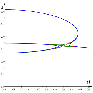
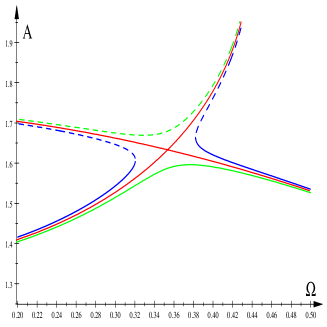
Figure 1: Amplitude profiles, $f=1$ ( singular, red), $f=0.999$ (green), and $f=1.001$ (blue) – left, neighborhood of the singular point, unstable branches marked by dashed lines – right.

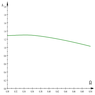
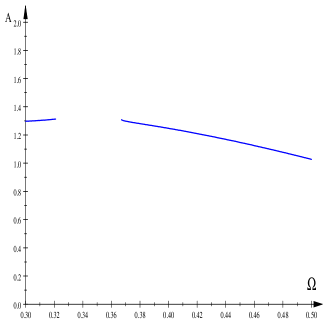
Figure 2: Bifurcation diagrams, $f=1.060$, left (green) and $f=1.061$, right (blue)

The corresponding amplitude profile, as well as two non-singular curves, are shown in Fig. 1. The singular curve (red) corresponds to self-intersection. The corresponding bifurcation diagrams, computed by numerical integration of the differential equation (2), $n=3$, are shown in Fig. 2.

It follows that there is indeed a gap on the bifurcation diagram (blue), corresponding to discontinuity on the amplitude profile (blue). In the case of numerical computation the discontinuity occurred for $1.060<f<1.061$, in good agreement with the predicted value $f=1$.

6 Examples of bifurcations at singular points of the amplitude profile for the cubic-quintic Duffing equation

It follows from Eqs. (30) that the cubic-quintic equation has a degenerate singular point for $c_{3}<0$. Moreover, in the neighbourhood of this point there are two families of non-degenerate singular points: isolated points and self-intersections.

Choosing, for example, $h=0.2$, $c_{3}=-0.2$, we compute from ((30) other parameters of the degenerate singular point as $c_{5}=1.\,212\,121\times 10^{-2}$, $f=0.295\,161$ and $\Omega=0.565\,685$, $A=2.\,569\,047$.

Now, for $h=0.2$, $c_{3}=-0.2$ and $c_{5}=1.15\times 10^{-2}$, we compute from Eqs. (16) for $n=5$: $f=0.282\,240$ – an isolated singular point with $\Omega=0.472\,685$, $A=2.\,920\,851$ and $f=0.290\,089$ – a self-intersection with $\Omega=0.617\,184$, $A=2.\,319\,843$.

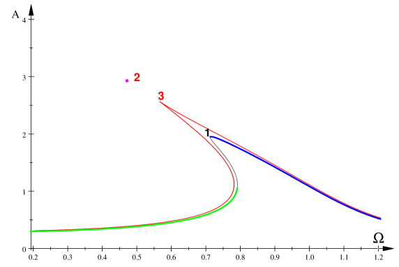
Figure 3: Amplitude profiles: degenerate, $c_{5}=1.\,212\,121\times 10^{-2},f=0.295\,161$ (red), isolated point, $c_{5}=1.15\times 10^{-2},$ $f=0.282\,240$ (green, blue, magenta)

The corresponding amplitude profiles for the degenerate and the isolated point are shown in Fig. 3. Green, blue and magenta colours have been used to show correspondence with bifurcation diagrams computed numerically near the isolated point, see Fig. 4. In the case of numerical integration of the Duffing equation (2), see C for computational details, an isolated point appears for $0.2990<f<0.2991$ in good agreement with the predicted value ($f=0.282\,240$).

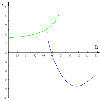
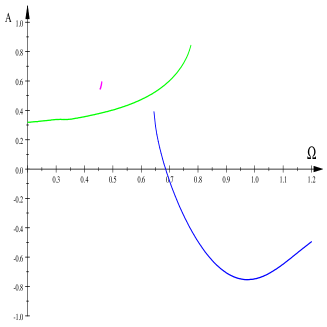
Figure 4: Bifurcation diagrams, $f=0.2990$ left – before the isolated point is formed, $f=0.2991$ right – just after formation of a new branch of solution (magenta). Colors (green, blue, magenta) correspond to colors in Fig. (3).

There are three characteristic points in Fig. (3 – solutions of Eq. (24). There is a cusp of the degenerate amplitude profile (red), singular with multiplicity $3$ – a triple solution of Eq. (24). Moreover there are two interesting points on the amplitude with isolated point (green, blue, magenta): an isolated point – singular with multiplicity $2$ (magenta dot) and a local maximum with multiplicity $1$ – non-singular and the corresponding bifurcation diagrams in Fig. 4 document indeed bifurcation due to metamorphosis of the amplitude profiles. The amplitude profile for the self-intersection is shown in Fig. 5

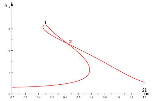
Figure 5: Amplitude profile, $h=0.2,$ $c_{3}=-0.2,$ $c_{5}=1.15\times 10^{-2},$ $f=290\,089$

and two amplitude profiles near the intersection are also shown in Fig. 6.

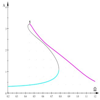
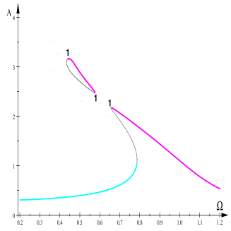
Figure 6: Amplitude profiles, $f=0.292$ (left, bofore the self-intersection), $f=0.289$ (right, after the self intersection).

The corresponding bifurcation diagrams document indeed bifurcation due to metamorphosis of the amplitude profiles.

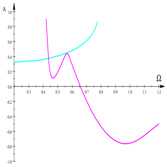
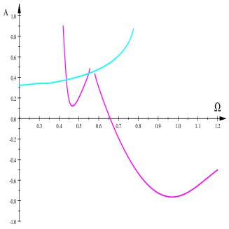
Figure 7: Bifurcation diagrams, $f=0.3026$ left, $f=0.3025$ right.

The bifurcation, discontinuity of the magenta line in Fig. 7, appears in numerical integration of the Duffing equation for $0.3025<f<0.3026$ in good agreement with the predicted value ($f=0.290\,089$).

7 Metamorphoses and bifurcations

7.1 Non-singular metamorphoses

It should be stressed that metamorphoses, i.e. changes of differential properties of asymptotic solutions, equivalent to bifurcations, occur also at nonsingular, yet critical, points of the amplitude-response equation. To show this let us consider the jump phenomenon for the Duffing equation [2, 15], see Fig. 8.

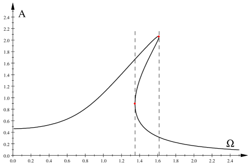
Figure 8: Jump phenomenon for the Duffing equation, $h=0.15$, $c_{3}=0.5$, $f=0.5$.

In two points marked with red dots, $\left(1.\,349,\ 0.894\right)$, $\left(1.\,615,\ 2.\,058\right)$, which are solutions of Eqs. (37), metamorphoses occur – a number of branches of the asymptotic solution is changed [15]. Real solutions appear for $h<0.304$, $c_{3}=0.5$, $f=0.5$, see [15] for analytical condition. It was determined by Kalmár-Nagy and Balachandran that this metamorphoses follows from a differential condition [2]:

$$\frac{d\Omega}{dA}=0$$ (33)

where the amplitude-response curve for the cubic Duffing equation is $F\left(\Omega,A\right)=L_{3}\left(\Omega^{2},A^{2}\right)=h^{2}A^{2}\Omega^{2}+A^{2}\left(\Omega^{2}-1-\frac{3}{4}c_{3}A^{2}\right)^{2}-f^{2}=0$ and is equivalent to the saddle-node bifurcation since one eigenvalue of the Jacobian matrix is zero, while another is negative. These metamorphoses can be also referred to as vertical tangencies of the response curve [2, 17].

The condition (33) can be formulated within the framework of implicit function theorem. Consider implicit amplitude response curve:

$$F\left(\Omega,\ A\right)=0.$$ (34)

Let $\Omega=f\left(A\right)$. Then:

$$\frac{\partial F}{\partial\Omega}\dfrac{d\Omega}{dA}+\frac{\partial F}{\partial A}\dfrac{dA}{dA}=0,$$ (35)

and

$$\dfrac{d\Omega}{dA}=f^{\prime}\left(A\right)=-\frac{\frac{\partial F}{\partial A}}{\frac{\partial F}{\partial\Omega}},\quad\left(\tfrac{\partial F}{\partial\Omega}\neq 0\right),$$ (36)

see Section 11.5 in [21].

Therefore, critical points of the function $\Omega=f\left(A\right)$, i.e. vertical tangencies, which follow from the Kalmár-Nagy and Balachandran condition $\dfrac{d\Omega}{dA}=f^{\prime}\left(A\right)=0$, fulfill an equivalent set of equations:

$$F\left(\Omega,\ A\right) = 0,$$ (37a)

$$\frac{\partial F\left(\Omega,\ A\right)}{\partial A} = 0.$$ (37b)

7.2 Singular metamorphoses

Singular points of the amplitude-response curves fulfill equations (13).

The first and third of these equations are conditions for vertical tangencies (37), associated with saddle-node bifurcations [2]. Therefore, because of the additional condition (13b), singular points of the amplitude-response curves lead to more complicated metamorphoses of these curves, discussed in Sections 5, 6.

On the other hand, also singular metamorphoses, due to Eq. (13c), are associated with saddle-node bifurcations. A connection between metamorphoses and bifurcations is revealed by computation of determinant of the Jacobian matrix $\mathbb{J}$. It follows from Eqs. (15), (7) that

$$\det\left(\mathbb{J}\right)=\frac{1}{4X}\frac{\partial L}{\partial Y},$$ (38)

where, for simplicity, the determinant is written in variables $X=\Omega^{2}$, $Y=A^{2}$.

It now follows that condition $\frac{\partial L\left(X,\ Y\right)}{\partial Y}=0$ $\left(\text{or }\frac{\partial L\left(\Omega^{2},\ A^{2}\right)}{\partial A}=0\right)$, defining a vertical tangency, is equivalent to vanishing of the determinant $\det\left(\mathbb{J}\right)$, and this means that at least one eigenvalue of the Jacobian matrix is zero, indicating a bifurcation.

We have computed another eigenvalue of the Jacobian matrix and in all cases considered it was equal $-h$. Therefore all bifurcations described in Sections 5, 6 are saddle-node bifurcations of co-dimension one.

8 Summary and discussion

In this work, we have studied changes of differential properties – metamorphoses – of amplitude response curves for the generalized Duffing equation with polynomial nonlinearities (1). We have demonstrated that metamorphoses are due to formation of singular points on amplitude profiles (the case of singular metamorphoses) and due to formation of critical points on these curves (the case of non-singular metamorphoses). The non-singular case, first described in [2] as due to formation of vertical tangent points, leads to important jump phenomena [2, 15]. We discuss singular and non-singular metamorphoses and associated bifurcations in Section 7.

More precisely, we have derived formulae for singular points and bifurcation sets of the amplitude response equation for the generalized Duffing equation (1), $n=3,5,7,\ldots$. We have described singular metamorphoses for the cubic Duffing equation ($n=3$) and the cubic-quintic Duffing equation ($n=5$).

It is interesting that there is a singular point in the case of the standard Duffing equation, see the corresponding metamorphoses of the amplitude profile and change of dynamics, cf. Figs. 1, 2. However, the set of parameters for which such points exist is rather small and can be easily overlooked.

In the cubic-quintic equation, $n=5$, there are degenerate points for $c_{3}<0$ and two infinite sets of self-intersections and isolated points in the neighbourhoods of these points, see Figs. 3, 5, 6. Bifurcations diagrams show indeed changes of dynamics – birth of new branches of solutions, Fig. 4, and rupture of existing branches, Fig. 7.

Summing up, knowledge of metamorphoses, non-singular, as well as singular, permits prediction of changes of dynamics such as jump phenomena (due to vertical tangent points), birth of new branches of solutions (due to isolated points), and rupture of existing branches of solutions leading to gaps in bifurcation diagrams (due to self-intersections). Knowledge of degenerate singular points pinpoints regions in the parameter space with families of isolated points and self-intersections where very complicated dynamical phenomena can occur.

There is an alternative approach to singular points of amplitude profiles when the implicit function can be disentangled, see A and B.

In the A we show that the implicit equation $F\left(A,\Omega\right)=0$ can be solved for the cubic-quintic Dufing equation resulting in explicit expression for two branches in form $\Omega_{\pm}=f_{\pm}\left(A\right)$ (actually equation (8) can be solved for $\Omega$ for any $n$). Condition of intersection of these branches, $f_{+}\left(A\right)=f_{-}\left(A\right)$ leads to dynamically interested points, non-singular as well as singular. It is important, that this condition, Eq. (40), is equivalent to the equation (24), derived within a more general approach. Accordingly, all these points are single or multiple solutions of Eq. (24). Within this approach we describe metamorphoses of the amplitude profiles in a more detailed way.

We compare in the B the computed amplitude profiles for the cubic-quintic Duffing equation with analogous solutions obtained by Karahan and Pakdemirli [5] within the Multiple Scales Lindstedt Poincaré (MSLP) approach, obtaining a qualitative agreement.

Appendix A Cubic-quintic Duffing equation: alternative approach to singular points of amplitude profiles

Solving Eq. (23) for $\Omega$ we get two positive solutions:

$$\Omega_{\pm} = \tfrac{1}{4}\sqrt{\tfrac{2}{A}}\sqrt{f\left(A\right)\pm 2\sqrt{g\left(A\right)}}$$ (39a)

$$f\left(A\right) = 5c_{5}A^{5}+6c_{3}A^{3}+4A\left(2-h^{2}\right)$$ (39b)

$$g\left(A\right) = -10c_{5}A^{6}h^{2}-12c_{3}A^{4}h^{2}+4A^{2}h^{2}\left(h^{2}-4\right)+16f^{2}$$ (39c)

The branches (39a) intersect for

$$g\left(A\right)=-10c_{5}A^{6}h^{2}-12c_{3}A^{4}h^{2}+4A^{2}h^{2}\left(h^{2}-4\right)+16f^{2}=0$$ (40)

It follows that $g\left(A\right)=-2f_{5}\left(A^{2}\right)$, cf. Eq. (24), and thus conditions $g\left(A\right)=0$ and $f_{5}\left(A^{2}\right)=0$ are equivalent.

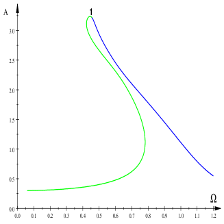
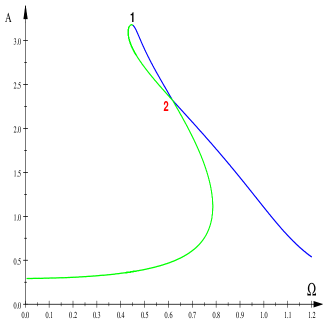
Figure 9: Amplitude profiles: $f=0.295$ left, $f=0.290\,089$ right

In Figs. 9, 10 transition from non-singular amplitude profile to self-intersection, to nonsingular profile, and to an isolated point is shown for $h=0.2$, $c_{3}=-0.2$, $c_{5}=0.0115$, and values of $f$ shown in the Figures.

Branches $\Omega_{+}$ and $\Omega_{-}$ are colored blue and green, respectively, black and red digits in the Figures denote multiplicity of the intersections of the branches (i.e. multiplicity of solutions of Eq. (40)) and correspond to non-singular and singular cases, respectively.

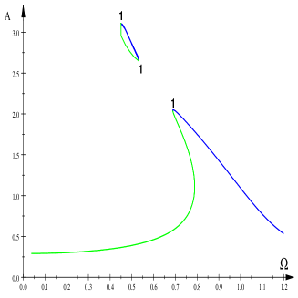
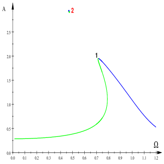
Figure 10: Amplitude profiles: $f=0.286$ left, $f=0.282\,25$ right

Note that this approach works for the generalized Duffing equation (2) for any $n$ since the amplitude equation (8) can be solved for $\Omega$ for an arbitrary $n$.

Appendix B Comparison with asymptotic solution from Ref. [5]

The cubic-quintic Duffing equation was also solved by application of Multiple Scales Lindstedt Poincaré (MSLP) method by Karahan and Pakdemirli, see Eqs. (89), (90) in [5]. The authors computed explicit solution as a function $\Omega=f\left(A\right)$ consisting of two branches:

$$\frac{\Omega_{\pm}}{\omega} = 1+\varepsilon^{2}\left(\dfrac{3\alpha^{3}}{256\omega^{4}}A^{4}+\dfrac{10\beta}{32\omega^{2}}A^{4}\pm\frac{1}{2}\sqrt{\dfrac{F^{2}}{A^{2}\omega^{4}}-\left(\dfrac{\mu}{\omega}\right)^{2}}\right)$$ (41a)

$$\omega = \sqrt{1+\varepsilon\frac{3}{4}\alpha A^{2}}$$ (41b)

Parameters used in [5] and our parameters are related:

$$h=\varepsilon^{2}\mu,\ c_{3}=\varepsilon\alpha,\ c_{5}=\varepsilon^{2}\beta,\ f=\varepsilon^{2}F$$ (42)

Condition for intersection of these branches is:

$$\dfrac{F^{2}}{A^{2}\omega^{4}}-\left(\dfrac{\mu}{\omega}\right)^{2}=0.$$ (43)

In Figures below $\varepsilon=1$, $\mu=h=0.2$, $\alpha=c_{3}=-0.2$, $\beta=c_{5}=0.0115$. Red digits indicate multiplicity of intersections of the branches (multiplicity of solutions of Eq. (43), branches $\omega_{+}$ and $\omega_{-}$ are colored blue and green, respectively.

Intersection of multiplicity $2$ appears for $F=f=0.258\,199$ what can be compared with the value obtained by numerical integration of the cubic-quintic Duffing equation $0.3025<f<0.3026$ (we have obtained from the KBM implicit function (23) value $f=290\,089$).

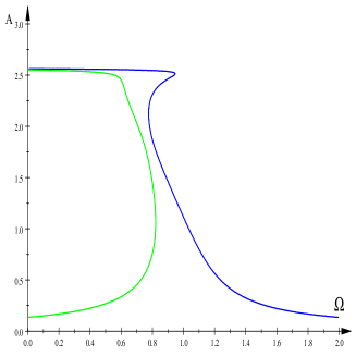
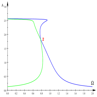
Figure 11: Amplitude profiles: $F=f=0.27$ left, $F=f=0.258\,199$ right

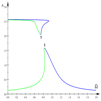
Figure 12: Amplitude profiles: $F=f=0.258\,199$ left, $F=f=0.25$ right

Alternatively, we can compute singular points writing Eq. (41a) in form $f\left(\Omega,A\right)=\pm\sqrt{g\left(\Omega,A\right)}$ to obtain implicit equation of form $K\left(\Omega,A\right)=f^{2}\left(\Omega,A\right)-g\left(\Omega,A\right)=0$ and applying standard equations:

$$K\left(\Omega,A\right) =0,$$ (44a)

$$\frac{\partial K\left(\Omega,A\right)}{\partial\Omega} =0,$$ (44b)

$$\frac{\partial K\left(\Omega,A\right)}{\partial A} =0.$$ (44c)

We can demonstrate within this approach that functions (41) do not have neither degenerate nor isolated points as singular solutions. It seems, however, that such points will be present if the MSLP solution contains higher-order terms.

Appendix C Computational details

Nonlinear polynomial equations were solved numerically using the computational engine Maple 4.0 from the Scientific WorkPlace 4.0. Figures were plotted with the computational engine MuPAD 4.0 from Scientific WorkPlace 5.5. Curves shown in bifurcation diagrams in Figs. 2, 4, 7 were computed by integrating numerically Eq. (2), $n=3,5$, running DYNAMICS, program written by Helena E. Nusse and James A. Yorke [22], and our own programs written in Pascal.

References

- [1] Kovacic, Ivana, Brennan, Michael J. (Eds.). The Duffing Equation: Nonlinear Oscillators and Their Behavior, John Wiley & Sons, 2011.
- [2] Kalmár-Nagy, T., & Balachandran, B. Forced harmonic vibration of a Duffing oscillator with linear viscous damping, in: The Duffing Equation: Nonlinear Oscillators and Their Behavior, John Wiley & Sons, 2011, pp. 139-174.
- [3] Mallik, Asok Kumar. Forced harmonic vibration of a Duffing oscillator with different damping mechanisms, in: The Duffing Equation: Nonlinear Oscillators and Their Behavior, John Wiley & Sons, 2011, pp. 175-217.
- [4] Younesian, D., Askari, H., Saadatnia, Z., and Kalami Yazdi, M. Frequency analysis of strongly nonlinear generalized Duffing oscillators using He’s frequency–amplitude formulation and He’s energy balance method. Comput. Math. Appl., 59 (2010) 3222-3228.
- [5] Karahan, MM Fatih, Pakdemirli M. Free and forced vibrations of the strongly nonlinear cubic-quintic Duffing oscillators, Zeit. Natur. A 72 (2017) 59-69.
- [6] Khatami, Iman, Ehsan Zahedi, and Mohsen Zahedi. Efficient solution of nonlinear Duffing oscillator. J. Appl. Comput. Mech. 6 (2020) 219-234.
- [7] Hieu, D. V., Hai, N. Q. Analyzing of nonlinear generalized Duffing oscillators using the equivalent linearization method with a weighted averaging. Asian Research Journal of Mathematics 9 (2018) 1-14.
- [8] Azimi, Alireza, Azimi, Mohammadreza. Computing Simulation of the Generalized Duffing Oscillator Based on EBM and MHPM. Mechanics and Mechanical Engineering 20 (2016) 595-604.
- [9] Zulli, D., Luongo, A. Control of primary and subharmonic resonances of a Duffing oscillator via non-linear energy sink, Int. J. Nonlinear Mech. 80 (2016) 170-182.
- [10] Bikdash, M., Balachandran, B., and Navfeh A.H. Melnikov analysis for a ship with a general roll-damping model, Nonlinear Dynamics 6 (1994) 101-124.
- [11] Nayfeh, A.H. Introduction to Perturbation Techniques, John Wiley & Sons, 2011.
- [12] Kyzioł, J., Okniński, A. Effective equation for two coupled oscillators: Towards a global view of metamorphoses of the amplitude profiles, Int. J. Nonlinear Mech. 123 (2020) 103495.
- [13] Spivak, M. Calculus on Manifolds, W.A. Benjamin, Inc., Menlo Park (California) 1965.
- [14] Wall, C.T.C. Singular Points of Plane Curves, Cambridge University Press, New York 2004.
- [15] Holmes, P.J., Rand, D.A. The bifurcations of Duffing’s equation: an application of Catastrophe Theory, J. Sound Vib. 44 (1976) 237-253.
- [16] Awrejcewicz, J. Modified Poincaré method and implicit function theory, in: Nonlinear Dynamics: New Theoretical and Applied Results, Awrejcewicz, J. (ed.), Akademie Verlag, Berlin, 1995, pp. 215-229.
- [17] Nayfeh, A.H., Balachandran, B. Applied nonlinear dynamics: analytical, computational, and experimental methods, John Wiley & Sons, 2008.
- [18] Kyzioł, J., Okniński, A. Van der Pol-Duffing oscillator: Global view of metamorphoses of the amplitude profiles, Int. J.Nonlinear Mech. 116 (2019) 102-106.
- [19] Gelfand, I.M., Kapranov, M.M., Zelevinsky, A.V. Discriminants, Resultants, and Multidimensional Determinants, Springer Science & Business Media, 2008.
- [20] Janson, S. Resultant and discriminant of polynomials, Lecture notes, http://www2.math.uu.se/~svante/papers/sjN5.pdf, 2010.
- [21] Stewart, J. Calculus: Concepts and contexts, Brooks/Cole, Cengage Learning, 2009.
- [22] Nusse, H.E., Yorke, J.A. Dynamics: Numerical Explorations, Springer Verlag New York Inc, 1997.