Fast and Accurate Amplitude Demodulation
of Wideband Signals

Abstract

Amplitude demodulation is a classical operation used in signal processing. For a long time, its effective applications in practice have been limited to narrowband signals. In this work, we generalize amplitude demodulation to wideband signals. We pose demodulation as a recovery problem of an oversampled corrupted signal and introduce special iterative schemes belonging to the family of alternating projection algorithms to solve it. Sensibly chosen structural assumptions on the demodulation outputs allow us to reveal the high inferential accuracy of the method over a rich set of relevant signals. This new approach surpasses current state-of-the-art demodulation techniques apt to wideband signals in computational efficiency by up to many orders of magnitude with no sacrifice in quality. Such performance opens the door for applications of the amplitude demodulation procedure in new contexts. In particular, the new method makes online and large-scale offline data processing feasible, including the calculation of modulator-carrier pairs in higher dimensions and poor sampling conditions, independent of the signal bandwidth. We illustrate the utility and specifics of applications of the new method in practice by using natural speech and synthetic signals.

I Introduction

Amplitude demodulation refers to the decomposition of a signal into a product of a slow-varying modulator-envelope and a fast-varying carrier. First introduced in radio communications [1], this procedure has found applications in data acquisition and processing related to a broad range of phenomena. Automatic speech recognition [2], atomic force microscopy [3], ultrasound imaging [4], brainwave [5], seismic trace [6], and fingerprint [7] analyses are a few among many examples to mention.

Originally, amplitude demodulation was intended for use with signals built of locally sinusoidal, i.e., narrowband, carri-ers. Several classical approaches excel in this setting, with Gabor’s analytic-signal (AS) method being a long-standing champion [8, 9]. Nonetheless, many relevant problems inevitably require demodulating signals that feature wideband carriers, typically of (quasi)-harmonic, (quasi)-random, or spike-train origin [10, 11, 12, 13, 14, 15, 16, 17, 18] (see Suppl. Mat. H for an overview). When applied to them, the classical techniques fail, misleadingly mixing the carrier and modulator information [19, 20].

For a long time, no consistent and accurate way of demodulating wideband signals was known. Typically, a proxy of the modulator would be obtained by rectifying and then low-pass filtering the signal. Different implementations of this procedure, each adapted for a specific signal class, were suggested (see, e.g., [21, 22, 17]). The estimates of signal modulators obtained in this way, however, are neither accurate nor consistent between different methods. The carriers and modulators are not appropriately separated either, i.e., they can be demodulated further by iterating the same procedure [23]. Moreover, the carrier estimates are often unbounded, even in well-defined situations (see, e.g., [23, Fig. 3.1]).

Recently, two promising demodulation approaches suitable to signals with arbitrary bandwidths have been formulated. Turner and Sahani shaped demodulation into a statistical inference problem [23, 24]. In this so-called probabilistic amplitude demodulation (PAD) approach, the modulator and carrier are inferred from the signal as latent variables of an appropriately selected statistical model. Mathematically, PAD defines a maximization of a posteriori probability, a high-dimensional nonlinear optimization task. In another work, Sell and Slaney chose a deterministic route to demodulation [19]. In their linear-domain convex (LDC) approach, the modulator is described as a minimum-power signal with penalized high-frequency terms lying above the original waveform. This problem is convex and thus amenable to more efficient optimization methods than the PAD.

The PAD and LDC techniques separate the modulator and carrier information of various synthetic wideband signals with a high degree of accuracy [23, 19]. The principal weakness of these approaches is a huge associated computational burden, which impedes their use in practical situations (see Section IV for the performance evaluations). In particular, online or large-scale offline signal processing is out of reach for the PAD and LDC demodulations. Besides, derivations of these methods are guided more by high-level modulator or carrier properties and computational tractability rather than strict recovery conditions. Hence, the boundaries of their validity in the context of real-world signals are somewhat blurred.

In this work, we frame demodulation as a problem of modulator recovery from an unlabeled mix of its true and corrupted sample points. We show that, under some loose constraints on carriers and modulators, high-accuracy demodulation can be achieved through exact or approximate norm minimization. We introduce different versions of custom-made alternating projection algorithms and test them in numerical experiments to solve this task. The new approach is shown to be free of the performance limitations inherent to the PAD and LDC methods. In particular, it combines the computational economy of the classical AS technique with the capacity to recover a wide range of arbitrary-bandwidth signals. We reveal the power of the new approach in terms of efficiency, accuracy, consistency, and robustness to corrupted data through theoretical analysis and illustrate it using synthetic signals with known structure. The use of the new method in realistic online and offline settings is demonstrated by applying it to natural speech.

II Mathematical Formulation of the Problem

In what follows, we assume the representation of a real-valued signal $s(t)$ formed by a finite collection of its values uniformly sampled over a limited time interval: $s_{i}\equiv s(t_{i})$, $i\in\mathcal{I}_{n}=\{1,2,\ldots,n\}$. Thus, a realization of the signal, $\mathbf{s}\equiv(s_{1},s_{2},\ldots,s_{n})^{T}$, is an element of an $n$-dimensional Euclidean space $\mathbb{R}^{n}$, i.e., a linear space equipped with the inner product $\langle\mathbf{s}^{(1)},\mathbf{s}^{(2)}\rangle=\sum_{i=1}^{n}(s^{(1)}_{i}\cdot s^{(2)}_{i})$, which induces the Euclidean norm $\|\mathbf{s}\|_{2}=\sqrt{\langle\mathbf{s},\mathbf{s}\rangle}$. We use modulo $n$ arithmetic for indexes of vector components in this work.

II-A Demodulation constraints

The task of demodulation is to factorize a signal $\mathbf{s}\in\mathbb{R}^{n}$ into a modulator $\mathbf{m}\in\mathbb{R}^{n}$ and a carrier $\mathbf{c}\in\mathbb{R}^{n}$:

$$\mathbf{s}=\mathbf{m}\circ\mathbf{c},$$ (1)

where symbol $\circ$ denotes an elementwise product of two vectors. There exists an uncountable number of pairs of $\mathbf{m}$ and $\mathbf{c}$ that satisfy (1). Thus, further constraints are needed to define its unique solution. It is precisely these constraints that give a distinct character to different demodulation methods and set the domain of their validity [9, 25, 23, 19].

In this work, we introduce the extra demodulation restrictions by imposing some general assumptions on $\mathbf{m}$ and $\mathbf{c}$.

We define feasible modulators as elements of a convex set

$$\mathcal{M}_{\omega}=\mathcal{S}_{\raisebox{0.9pt}{\scalebox{0.5}{$\geq$}\raisebox{-0.95pt}{\scalebox{0.65}{$\mathbf{0}$}}}}\cap\mathcal{S}_{\omega},$$ (2)

where

$$\mathcal{S}_{\raisebox{0.9pt}{\scalebox{0.5}{$\geq$}\raisebox{-0.95pt}{\scalebox{0.65}{$\mathbf{0}$}}}} =\{\mathbf{x}\in\mathbb{R}^{n}:x_{i}\geq 0,\,i\in\mathcal{I}_{n}\},$$

$$\mathcal{S}_{\omega} =\{\mathbf{x}\in\mathbb{R}^{n}:(\mathbf{F}\mathbf{x})_{i}=0,\,i\in(\mathcal{I}_{n}\setminus\mathcal{I}_{n}^{\omega})\},$$ (3)

$$\mathcal{I}_{n}^{\omega} =\{i\in\mathcal{I}_{n}:i\leq\omega\}\cup\{i\in\mathcal{I}_{n}:i>n+1-\omega\}.$$

In (3), $\mathbf{F}$ denotes the operator of the unitary discrete Fourier transform (DFT), and $(\ldots)_{i}$ marks the $i$-th component of the argument vector. Hence, in our framework, modulators are nonnegative low-pass signals whose rate of variation is limited by the cutoff frequency $\omega$ (with $1\leq\omega\leq\lceil n/2\rceil$), which parametrizes $\mathcal{M}_{\omega}$. This is a formal definition of the classical modulator-envelope [1, 26].

We declare feasible carriers as elements of a nonconvex set

$$\mathcal{C}_{d}=\mathcal{S}_{\raisebox{1.0pt}{\scalebox{0.5}{$|..|\leq$}}\scalebox{0.67}{$\mathbf{1}$}}\cap\mathcal{S}_{\raisebox{1.0pt}{\scalebox{0.45}{\{}}\raisebox{0.27pt}{\scalebox{0.55}{1}}\raisebox{1.0pt}{\scalebox{0.45}{\}}},d},$$ (4)

where

$$\mathcal{S}_{\raisebox{1.0pt}{\scalebox{0.5}{$|..|\leq$}}\scalebox{0.67}{$\mathbf{1}$}} =\{\mathbf{x}\in\mathbb{R}^{n}:|x_{i}|\leq 1,\,i\in\mathcal{I}_{n}\},$$ (5)

$$\mathcal{S}_{\raisebox{1.0pt}{\scalebox{0.45}{\{}}\raisebox{0.27pt}{\scalebox{0.55}{1}}\raisebox{1.0pt}{\scalebox{0.45}{\}}},d} =\big{\{}\mathbf{x}\in\mathbb{R}^{n}:{\textstyle(\forall i)\sum_{j=i}^{i+d-1}I_{\{1\}}(|x_{j}|)\geq 1,}$$

$$\hskip 59.0pt{\textstyle(\exists i)\sum_{j=i}^{i+d-1}I_{\{1\}}(|x_{j}|)=1}\big{\}},$$

with $I_{\{1\}}$ being the indicator function of the singleton $\{1\}$. The set $\mathcal{S}_{\raisebox{1.0pt}{\scalebox{0.5}{$|..|\leq$}}\scalebox{0.67}{$\mathbf{1}$}}$ implies the boundedness of $\mathbf{c}$ between $-1$ and $1$. This restriction follows from the standard notion that the time-dependent amplitude of an amplitude-modulated $\mathbf{s}$ is purely set by $\mathbf{m}$. Meanwhile, $\mathcal{S}_{\raisebox{1.0pt}{\scalebox{0.45}{\{}}\raisebox{0.27pt}{\scalebox{0.55}{1}}\raisebox{1.0pt}{\scalebox{0.45}{\}}},d}$ fixes to $d$ the maximum gap between any two neighboring components of $\mathbf{c}$ whose absolute values are equal to $1$. As shown next, this constraint allows formulating extensive demodulation guarantees while only moderately affecting the scope of relevant carriers. Bandwidth-wise, $\mathcal{C}_{d}$ covers the whole range, from zero (sinusoidal) to flat (random spike) bandwidth signals, and defines the qualifier “wideband” used in this work. Note that the bandwidth of $\mathbf{c}\in\mathcal{C}_{d}$ is mostly determined not by $d$ but by the arrangement of the $|c_{i}|=1$ and other sample points. Instead, as we see next, $d$ decides whether a chosen $\mathbf{c}\in\mathcal{C}_{d}$ can be restored after modulation.

II-B Demodulation as modulator recovery

Note that, assuming $\mathbf{c}\in\mathcal{C}_{d}$, $|\mathbf{s}|$ can be seen as a corrupted version of $\mathbf{m}$: $|s_{i}|=m_{i}$ when $|c_{i}|=1$, and $|s_{i}|\neq m_{i}$ otherwise. Further, if $\mathbf{m}$ can be found from $|\mathbf{s}|$, $\mathbf{c}$ follows from (1) uniquely ($c_{i}=s_{i}/m_{i}$), except the sample points with $m_{i}=0$. The latter, if any, are sparse and can be typically interpolated from the neighboring points. Hence, in our case, demodulation is virtually a problem of reconstructing $\mathbf{m}$ from a mix of its true ($i:|s_{i}|=m_{i}$) and corrupted ($i:|s_{i}|\neq m_{i}$) sample points when the class of each point is unknown. This viewpoint is at the core of the developments that follow next.

II-C Modulator recovery through norm minimization

Our approach to demodulation builds around the estimator

$$\mathbf{\hat{m}}=\underset{\mathbf{x}\in\mathcal{S}_{\raisebox{1.0pt}{\scalebox{0.4}{$\geq|$}\scalebox{0.52}{$\mathbf{s}$}\scalebox{0.4}{$|$}}}\cap\mathcal{S}_{\varpi}}{\arg\min}\|\mathbf{x}\|_{2},$$ (6)

where $\mathcal{S}_{\raisebox{1.0pt}{\scalebox{0.5}{$\geq|$}\scalebox{0.72}{$\mathbf{s}$}\scalebox{0.5}{$|$}}}=\{\mathbf{x}\in\mathbb{R}^{n}:x_{i}\geq|s_{i}|,i\in\mathcal{I}_{n}\}$. Note that $\mathbf{m}\in$ $\mathcal{S}_{\raisebox{1.0pt}{\scalebox{0.5}{$\geq|$}\scalebox{0.72}{$\mathbf{s}$}\scalebox{0.5}{$|$}}}\cap\mathcal{S}_{\varpi}$ if $\varpi\geq\omega$. The restriction corresponding to $\mathcal{S}_{\raisebox{1.0pt}{\scalebox{0.5}{$\geq|$}\scalebox{0.72}{$\mathbf{s}$}\scalebox{0.5}{$|$}}}$ assures that $\mathbf{x}$ does not fall below $\mathbf{m}$ at the true sample points, i.e., points where $m_{i}=|s_{i}|$. If, besides, the true sample points are spread densely enough, we expect the norm minimization to enforce $\hat{m}_{i}=m_{i}$ at these points. But then, $\mathbf{\hat{m}}=\mathbf{m}$ by the discrete sampling theorem. The foundation for this intuitive consideration is laid by the following results (see Suppl. Mat. B for the proofs).

Proposition II.1.

For almost every $\mathbf{m}\in\mathcal{M}_{\omega}$, $\mathbf{\hat{m}}=\mathbf{m}$ only if $\varpi\geq\omega$, and $\mathbf{c}\in\mathcal{C}_{d}$ with $n_{s}\equiv\sum_{i=1}^{n}I_{\{1\}}(|c_{i}|)\geq\varpi+\omega-1\implies d\leq n-(\varpi+\omega-2)$.

Proposition II.2.

Consider $\mathbf{m}\in\mathcal{M}_{\omega}$ and $\mathbf{\tilde{c}}\in\mathcal{C}_{\tilde{d}}$ with $|\tilde{c}_{i}|=1$ for $i\in\mathcal{J}_{n}\subseteq\mathcal{I}_{n}$, and $\tilde{c}_{i}=0$ otherwise. If $\mathbf{\hat{m}}=\mathbf{m}$ holds for the $\mathbf{m}$ and $\mathbf{\tilde{c}}$, then it also holds for every pair made of the same $\mathbf{m}$ and any $\mathbf{c}\in\mathcal{C}_{d}$ with $d\leq\tilde{d}$ and $|c_{i}|=1$ for $i\in\mathcal{J}_{n}$.

Proposition II.3.

Assume $\mathbf{m}\in\mathcal{M}_{\omega}$ and $\mathbf{c}\in\mathcal{C}_{d}$ with $\varpi\geq\omega$. If, additionally, there exist $d\in\mathcal{I}_{n}$ and $i\in\mathcal{I}_{d}$ such that $n_{s}\equiv(n/d)\in\mathbb{N}_{+}$, $n_{s}\geq\varpi+\omega-1$, and $|c_{i+(j-1)\cdot d}|=1$ for every $j\in\mathcal{I}_{n_{s}}$, then $\mathbf{\hat{m}}=\mathbf{m}$.

Proposition 3 reveals the tight match of $\mathbf{\hat{m}}$ to $\mathcal{C}_{d}$: no $\mathbf{m}\in\mathcal{M}_{\omega}$ can be inferred from $\mathbf{s}$ by $\mathbf{\hat{m}}$ precisely if $\mathbf{c}\notin\mathcal{C}_{d}$. It also establishes the central role of the presence of true sample points in the recovery: for almost every $\mathbf{m}\in\mathcal{M}_{\omega}$, at least the number $\varpi+\omega-1$ of such points is needed. Proposition II.2 further consolidates the latter view by stating that the success of the exact recovery of an $\mathbf{m}\in\mathcal{M}_{\omega}$ via $\mathbf{\hat{m}}$ is fully determined by the number and positions of the true sample points. In particular, if exact demodulation is possible for some $\mathbf{\tilde{c}}$ with $\tilde{c}_{i}\in\{0,1\}$, then it is possible for any $\mathbf{c}$ with $|c_{i}|=1$ at $i\in\{j:\tilde{c}_{j}=1\}$ independent of other sample points.

In Proposition 3, $\varpi\geq\omega$ and $n_{s}\geq\varpi+\omega-1$ imply $n_{s}\geq 2\omega-1$, which is a sufficient condition for $\mathbf{m}$ recovery in the classical setup when all true sample points are known (see the remark below the proof of Proposition A.1 in Suppl. Mat. A). Hence, the data corruption manifesting in our problem necessitates further constraints on the number or positions of true sample points. In particular, Proposition II.3 certifies a full recovery of $\mathbf{m}$ if $\varpi\geq\omega$, and there exists a (not necessarily known) subset of at least $\varpi+\omega-1$ regularly-spaced true sample points. The latter condition covers a wide range of practically relevant carriers, including: (1) the classical $\sin(2\pi\nu\mathbf{t}+\phi)$ with $\nu\geq\omega$, (2) harmonic signals, (3) regular spike-trains of $|c_{i}|=1$. More generally, any (non)stationary time-series with regularly placed $|c_{i}|=1$ regardless of the remaining points are eligible.

In addition to the regularity of true sample points, Proposition II.3 requires $n/d$ to be an integer. Nevertheless, numerical experiments reveal that both of these conditions can be ignored without practically relevant consequences (see Suppl. Mat. C and Fig. 10 there). In particular, we found that the discrepancy between $\mathbf{m}$ and $\mathbf{\hat{m}}$ is vanishing with an overwhelming probability for any $\mathbf{c}\in\mathcal{C}_{d}$ if $\varpi\geq\omega$, and $\lceil n/d\rceil\geq 2\varpi-1$. This result noticeably extends the scope of recovery conditions over the domain of practically relevant (quasi-)regular and stochastic carriers. Among the examples are nonstationary sinusoidal and harmonic signals and arbitrary spike-trains with the distance between neighboring spikes at or below $d$ points. Note that $n_{s}\geq\lceil n/d\rceil$ by the definition of $\mathcal{C}_{d}$. Hence the relaxation of the strict regularity condition on the $|c_{i}|=1$ sample points comes at the expense of a slightly tighter constraint on $n_{s}$ necessary for exact recovery of $\mathbf{m}$: compare $n_{s}\geq 2\varpi-1$ vs. $n_{s}\geq\varpi+\omega-1$.

Another important generalization of the recovery conditions comes with the following inequality:

Proposition II.4.

Consider $\mathbf{m}\in\mathcal{M}_{\omega}$ and $\mathbf{c}\in\mathcal{S}_{\raisebox{1.0pt}{\scalebox{0.5}{$|..|\leq$}}\scalebox{0.67}{$\mathbf{1}$}}$. Take $n_{s}\geq 2\varpi-1$ sample points of $\mathbf{s}=\mathbf{m}\circ\mathbf{c}$ whose indexes are defined as entries of any chosen $\mathbf{r}\in\mathbb{N}_{+}^{n_{s}}$ with $r_{i+1}-r_{i}=n/n_{s}$ for every $i\in\mathcal{I}_{n_{s}}$. Then,

$$\textstyle\|\mathbf{m}-\mathbf{\hat{m}}\|_{2}/\|\mathbf{m}\|_{2}\leq\sqrt{1-\sum_{i=1}^{n_{s}}s_{r_{i}}^{2}/\sum_{i=1}^{n_{s}}m_{r_{i}}^{2}}.$$ (7)

Hence, if one can find a sequence of at least $2\varpi-1$ regularly-spaced sample points with $|s_{i}|$ sufficiently close to $m_{i}$, then the relative recovery error is close to 0 in terms of (7). This result endows $\mathbf{\hat{m}}$ with the stability to discrepancies from the recovery conditions discussed earlier. At the same time, it provides approximate recovery guarantees for a wider range of stochastic and (quasi-)regular carriers besides those with fairly densely packed $|c_{i}|=1$ sample points. Due to the low-pass restriction on $\mathbf{m}$, (7) is expected to hold approximately for an irregular $\mathbf{r}\in\mathbb{N}_{+}^{n_{s}}$ with $r_{i+1}-r_{i}\leq\lceil n/n_{s}\rceil$ as well.

We finally note that, whereas $\omega$ and $d$ are fixed properties of $\mathbf{m}$ and $\mathbf{c}$, $\varpi$ is a control parameter that must be specified. An appropriate $\varpi$, which satisfies the recovery conditions formulated above, can only be selected by using prior knowledge on $\mathbf{m}$ and $\mathbf{c}$ or found in a supervised learning setup.

II-D Relaxation of the exact minimum-norm requirement

The norm-minimizing property of $\mathbf{\hat{m}}$ in (6) is critical in formulating sharp recovery conditions. However, from a practical point of view, little would be lost if another estimator $\mathbf{\hat{m}}$ with only slightly larger than the minimum norm among all elements of $\mathcal{S}_{\raisebox{1.0pt}{\scalebox{0.5}{$\geq|$}\scalebox{0.72}{$\mathbf{s}$}\scalebox{0.5}{$|$}}}\cap\mathcal{S}_{\varpi}$ is used. Thus, we relax (6) to

find $$\qquad\mathbf{\hat{m}}\in\mathcal{S}_{\raisebox{1.0pt}{\scalebox{0.5}{$\geq|$}\scalebox{0.72}{$\mathbf{s}$}\scalebox{0.5}{$|$}}}\cap\mathcal{S}_{\varpi}$$ (8)

subject to $$\qquad\|\mathbf{\hat{m}}\|_{2}\simeq\underset{\mathbf{x}\in\mathcal{S}_{\raisebox{1.0pt}{\scalebox{0.4}{$\geq|$}\scalebox{0.52}{$\mathbf{s}$}\scalebox{0.4}{$|$}}}\cap\mathcal{S}_{\varpi}}{\arg\min}\|\mathbf{x}\|_{2}$$

To specify the otherwise ambiguous relation operator $\simeq$, we request that $\mathbf{\hat{m}}$ obtained through (8) recovers $\mathbf{m}$ exactly, i.e., is norm-minimizing, for sinusoidal, harmonic, and spike-train carriers covered by Proposition II.3. As we see later, this restriction regularizes the numerical algorithms formulated in the present work for sufficiently accurate demodulation well beyond those three classes of $\mathbf{c}$. The advantage brought by the approximation is computational efficiency.

II-E Method of solution

The algorithms that we introduce to solve (6) and (8) in this work fall in the domain of the so-called methods of alternating projections (APs). The defining feature of each AP method is an iterative calculation of a feasible point ($\mathbf{\hat{m}}\in\mathcal{S}_{\raisebox{1.0pt}{\scalebox{0.5}{$\geq|$}\scalebox{0.72}{$\mathbf{s}$}\scalebox{0.5}{$|$}}}\cap\mathcal{S}_{\varpi}$ in our case) via alternating metric projections of its current estimate onto the separate constraint sets. Initially proposed by von Neumann for two closed subspaces [27], this approach was later extended to arbitrary closed convex sets of a Hilbert space (see [28] for a review). Various implementations of the AP algorithms exist, featuring different domains of application, rate of convergence, and additional requirements satisfied by the solutions [29, 28].

We provide a rigorous mathematical basis on which the AP algorithms for solving the demodulation problem rely in Suppl. Mat. D, E, F. For a practical comprehension of the material that follows next, it is sufficient to know that:

• The sets $\mathcal{S}_{\raisebox{1.0pt}{\scalebox{0.5}{$\geq|$}\scalebox{0.72}{$\mathbf{s}$}\scalebox{0.5}{$|$}}}$ and $\mathcal{S}_{\varpi}$ are closed and convex.

• A metric projection, or simply a projection henceforth, of $\mathbf{z}\in\mathbb{R}^{n}$ onto a closed convex set $\mathcal{S}\subset\mathbb{R}^{n}$ is a unique $\mathbf{x_{z}}\in\mathcal{S}$ with the smallest distance, i.e., $\|\mathbf{x_{z}}-\mathbf{z}\|_{2}$, from $\mathbf{z}$.

• The projections onto $\mathcal{S}_{\raisebox{1.0pt}{\scalebox{0.5}{$\geq|$}\scalebox{0.72}{$\mathbf{s}$}\scalebox{0.5}{$|$}}}$ and $\mathcal{S}_{\varpi}$ are respectively achieved by operators

  $$\mathbf{P}_{\mathcal{S}_{\raisebox{1.0pt}{\scalebox{0.4}{$\geq|$}\scalebox{0.52}{$\mathbf{s}$}\scalebox{0.4}{$|$}}}}[\mathbf{z}]=|\mathbf{s}|+(\mathbf{z}-|\mathbf{s}|)\circ\theta(\mathbf{z}-|\mathbf{s}|)$$ (9)

  and

  $$\mathbf{P}_{\mathcal{S}_{\varpi}}[\mathbf{z}]=(\mathbf{F^{-1}}\,\mathbf{W}_{\varpi}\,\mathbf{F})\,\mathbf{z}.$$ (10)

  Here, $\theta(\ldots)$ is the Heaviside step function evaluated elementwise. $\mathbf{W}_{\varpi}$ is a diagonal matrix such that $(W_{\varpi})_{ii}=1$ if $i\in\mathcal{I}_{n}^{\varpi}$, and $(W_{\varpi})_{ii}=0$ otherwise.

To emphasize the nature of the underlying numerical algorithms, we name our new approach as AP demodulation.

II-F Relation to other problems and approaches

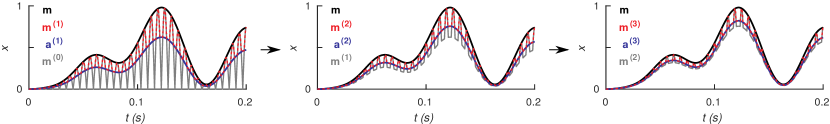
Figure 1: The first three iterations of the AP-B algorithm applied to an amplitude-modulated sinusoidal signal. $\mathbf{m}$ stands for the real modulator.

Demodulation is a counterpart of a widely known and studied problem of blind deconvolution: $\mathbf{s}=\mathbf{m}\,\raisebox{0.7pt}{{$\scriptstyle\circledast$}}\,\mathbf{c}$. Indeed, both tasks admit the algebraic form of each other in the Fourier domain. Nevertheless, the properties of $\mathbf{m}$ and $\mathbf{c}$ inherent to practical instantiations of amplitude demodulation and blind deconvolution differ significantly. These differences predetermine the need for distinctive strategies to solve the respective tasks, as discussed next.

One of the most powerful convex-programming-based deconvolution approaches, introduced in [30], builds on the assumption that $\mathbf{m}$ and $\mathbf{c}$ belong to known low-dimensional subspaces. There, recovery of $\mathbf{m}$ and $\mathbf{c}$ is achieved by minimiz-ing the nuclear, atomic, $\ell_{1}$, or $\ell_{2,1}$ norms of their outer product (in the subspace representation) subject to linear measurement constraints of $\mathbf{s}$ [30, 31, 32, 33]. This scheme successfully solves many practically relevant blind deconvolution cases, such as image deblurring, multipath channel protection, and super-resolution microscopy [30, 33]. However, the low-dimension subspace assumption, a crucial prerequisite of the approach, renders it inapt to deal with realistic carriers in the amplitude demodulation context. Indeed, even a sinusoidal carrier with a fluctuating phase is hardly representable in this frame, not to mention more complex wideband signals met in practice. Moreover, the subspace model of $\mathbf{m}$ and $\mathbf{c}$ does not allow enforcing the amplitude contents to $\mathbf{m}$ exclusively.

Deconvolution problems have also been approached by using AP-like methods [34, 35, 36, 37]. A general strategy of the existing algorithms is to achieve deconvolution by an iterative refinement of both $\mathbf{m}$ and $\mathbf{c}$ upon the requirement of exact [34, 36] or approximate [35, 37] adherence to the defining equality $\mathbf{s}=\mathbf{m}\,\raisebox{0.7pt}{{$\scriptstyle\circledast$}}\,\mathbf{c}$ and the support region, intensity range, and spectrum constraints implied on $\mathbf{m}$ and $\mathbf{c}$ or $\mathbf{r}=\mathbf{s}-\mathbf{m}\,\raisebox{0.7pt}{{$\scriptstyle\circledast$}}\,\mathbf{c}$. These methods differ significantly between themselves. Each of them achieves satisfactory recovery by a judicious combination of specific constraint sets and the iterative scheme adjusted to specific classes of $\mathbf{m}$ and $\mathbf{c}$. The nonconvexity of $\mathcal{C}_{d}$ and the absence of efficient explicit projections onto this set makes the application of the known deconvolution methods unsuitable to amplitude demodulation. None of the current AP-like deconvolution methods allow assigning the amplitude contents to $\mathbf{m}$ purely either.

We next note that our formulation of the amplitude demodulation problem in Section II-B reveals it as a generalization of the classical task of band-limited signal recovery from true sample points. An AP method known under the name Papoulis-Gerchberg and its variants were successfully applied in the latter setting (see [38] for a review). The differences in the available information on the recoverable signal lead to distinct strategies in algorithmic approaches to these two problems. In particular, the Papoulis-Gerchberg methods rely entirely on known true data. Thus, they are impossible to use for demodulation purposes. The AP algorithms introduced in the present work can be applied in the classical setting. However, not using the available information about the true data makes them inferior to their classical counterparts unless the sample points are fairly uniformly spread, as discussed in Section II-C.

The approach suggested in the present work also has some parallels with the LDC demodulation method by [19]. There, (1) is accompanied by a constraint on the modulator $\mathbf{m}$ expressed as the solution of the quadratic programming problem

minimize $$\qquad\|\mathbf{w}\circ\mathbf{F}\mathbf{m}\|_{2}^{2}+\|\mathbf{m}\|_{2}^{2}$$ (11)

subject to $$\qquad|s_{i}|\leq m_{i}\leq\max[\mathbf{s}]\qquad\forall i\in\mathcal{I}_{n},$$

where $\mathbf{w}$ denotes the weighting vector. (11) was introduced heuristically, trying to quantify the intuitive notion of the modulator-envelope as a signal wrapping $\mathbf{s}$ from above.

Practical applications suggest the LDC method defined by (1) and (11) being computationally most efficient and precise among all current techniques designed for demodulating signals unreachable to classical algorithms [24, 19]. Thus, we use it as a reference when evaluating the performance of the newly-formulated approach of the present work.

III Demodulation Algorithms

In this section, we formulate three algorithms representing the core arsenal of the AP approach to demodulation. Simplicity, efficiency, and estimation accuracy of the algorithms are the main aspects under consideration. We refer the reader to Suppl. Mat. F for proofs of all propositions found here.

III-A AP-Basic

We start with the simplest possible AP algorithm, therefore named “AP-Basic” (AP-B).

  Algorithm: AP-Basic (AP-B)  

1:  Set: $N_{iter}$, $\epsilon_{tol}$

2:  Initialize: $i=0$, $\epsilon^{(0)}=\|\mathbf{s}\|_{2}/\sqrt{n}$, $\mathbf{m}^{(0)}=|\mathbf{s}|$, $\mathbf{a}^{(0)}=\mathbf{0}$

3:  while $\epsilon^{(i)}>\epsilon_{tol}$ and $i<N_{iter}$ do

4:     $i=i+1$

5:     $\mathbf{a}^{(i)}=\mathbf{P}_{\mathcal{S}_{\varpi}}[\mathbf{m}^{(i-1)}]$

6:     $\mathbf{m}^{(i)}=\mathbf{P}_{\mathcal{S}_{\raisebox{1.0pt}{\scalebox{0.4}{$\geq|$}\scalebox{0.52}{$\mathbf{s}$}\scalebox{0.4}{$|$}}}}[\mathbf{a}^{(i)}]$

7:     $\epsilon^{(i)}=\|\mathbf{m}^{(i)}-\mathbf{a}^{(i)}\|_{2}/\sqrt{n}$

8:  end while

9:  Finalize: $\mathbf{\hat{m}}=\mathbf{m}^{(i)}$  

Here, $N_{iter}$ stands for the maximum number of algorithm iterations. $\epsilon^{(i)}$ is the infeasibility error at the $i$-th iteration, which is used to control the termination of the algorithm. Specifically, $\epsilon^{(i)}$ measures the distance of the modulator estimate $\mathbf{m}^{(i)}\in\mathcal{S}_{\raisebox{1.0pt}{\scalebox{0.5}{$\geq|$}\scalebox{0.72}{$\mathbf{s}$}\scalebox{0.5}{$|$}}}$ from $\mathcal{S}_{\varpi}$ and sets a lower bound on the convergence error: $\epsilon^{(i)}\leq\|\mathbf{m}^{(i-1)}-\mathbf{m}^{\dagger}\|_{2}/\sqrt{n}$ (see Suppl. Mat. G). The iterative process is stopped when $\epsilon^{(i)}$ drops to the level of a predetermined threshold $\epsilon_{tol}>0$ or below. $\epsilon_{tol}\leq 0$ would force the completion of all $N_{iter}$ iterations of the algorithm. $\mathbf{\hat{m}}$ denotes the final estimate of the modulator. $\mathbf{\hat{m}}$ arbitrarily close to $\mathcal{S}_{\raisebox{1.0pt}{\scalebox{0.5}{$\geq|$}\scalebox{0.72}{$\mathbf{s}$}\scalebox{0.5}{$|$}}}\cap\mathcal{S}_{\varpi}$ can be reached if $N_{iter}$ is sufficiently large:

Proposition III.1.

A sequence $\mathbf{m}^{(0)},\mathbf{m}^{(1)},\ldots,\mathbf{m}^{(i)},\ldots$ formed by the AP-B algorithm for $\epsilon_{tol}=0$ and $N_{iter}\to+\infty$ converges to some $\mathbf{m}^{\dagger}\in\mathcal{S}_{\raisebox{1.0pt}{\scalebox{0.5}{$\geq|$}\scalebox{0.72}{$\mathbf{s}$}\scalebox{0.5}{$|$}}}\cap\mathcal{S}_{\varpi}$. The convergence is geometric and monotonic, i.e., there exist $\gamma>0$ and $0<r<1$ such that $\|\mathbf{m}^{(i)}-\mathbf{m}^{\dagger}\|_{2}\leq\gamma\cdot r^{i}$ and $\|\mathbf{m}^{(i+1)}-\mathbf{m}^{\dagger}\|_{2}\leq\|\mathbf{m}^{(i)}-\mathbf{m}^{\dagger}\|_{2}$ for $i\geq 0$.

It can be shown by example that the AP-B does not always provide minimum-norm estimators $\mathbf{\hat{m}}$. However, it is expected to do so at least approximately if some conditions are met. We clarify this next with the help of Fig. 1, which displays the first three iterations of the AP-B applied to an example signal.

First, note that the starting point $\mathbf{m}^{(0)}$ is elementwise not-higher than the real modulator $\mathbf{m}$ (black). $\mathbf{P}_{\mathcal{S}_{\varpi}}$ maps $\mathbf{m}^{(0)}$ to $\mathbf{a}^{(1)}$, which, by definition of a metric projection, is its best mean-squared-error (MSE) approximation in $\mathcal{S}_{\varpi}$ (blue). By the definition of $\mathcal{S}_{\varpi}$, $\mathbf{a}^{(1)}$ is nearly constant over time windows shorter than $n/(2\pi\varpi)$ points. In general, the best constant MSE estimator of a sample of numbers is its average. Thus, as the best MSE estimator of $\mathbf{m}^{(0)}$ over $\mathcal{S}_{\varpi}$, $\mathbf{a}^{(1)}$ approximates the local average of $\mathbf{m}^{(0)}$ values in a window of $\approx n/(2\pi\varpi)$ points at every moment. If $\varpi\geq\omega$, $\mathbf{c}\in\mathcal{S}_{\raisebox{1.0pt}{\scalebox{0.5}{$|..|\leq$}}\scalebox{0.67}{$\mathbf{1}$}}$, and $\approx n/(2\pi\varpi)$ sample points are sufficient to average out the local variations of $\mathbf{c}$, $\mathbf{a}^{(1)}$ is supposed to be proportional to $\mathbf{m}$, at least roughly. The first iteration is completed by the projection of $\mathbf{a}^{(1)}$ back onto $\mathcal{S}_{\raisebox{1.0pt}{\scalebox{0.5}{$\geq|$}\scalebox{0.72}{$\mathbf{s}$}\scalebox{0.5}{$|$}}}$ to obtain $\mathbf{m}^{(1)}$ (red).

Applying the same reasoning as above, we deduce that, with each iteration, $\mathbf{a}^{(i)}$, and thus $\mathbf{m}^{(i)}$, approaches $\mathbf{m}$ elementwise (see Fig. 1). In general, $\mathbf{m}^{(i)}$ may exceed the level of the real modulator $\mathbf{m}$ over time windows longer than $\geq n/(2\pi\varpi)$ points for higher $i$ before $\mathbf{m}^{\dagger}\in\mathcal{S}_{\raisebox{1.0pt}{\scalebox{0.5}{$\geq|$}\scalebox{0.72}{$\mathbf{s}$}\scalebox{0.5}{$|$}}}\cap\mathcal{S}_{\varpi}$ is reached. However, as follows from the considerations of the previous paragraph, such segments of $\mathbf{m}^{(i)}$ would be approximately compatible with $\mathcal{S}_{\raisebox{1.0pt}{\scalebox{0.5}{$\geq|$}\scalebox{0.72}{$\mathbf{s}$}\scalebox{0.5}{$|$}}}\cap\mathcal{S}_{\varpi}$ and would not be considerably affected in subsequent iterations. Hence, $\mathbf{\hat{m}}$ obtained by the AP-B is expected to follow the true sample points of $\mathbf{m}$ tightly. If the number of these points is sufficient, then $\mathbf{\hat{m}}\simeq\mathbf{m}$ as well.

The basis for the above considerations is laid by the fact that they are exact for some important types of carriers:

Proposition III.2.

Consider $\mathbf{m}\in\mathcal{M}_{\omega}$ and $\mathbf{c}\in\mathcal{C}_{d}$ with $|c_{j}|=\sum_{k=1}^{n/\nu}(\tilde{c}_{\nu\cdot k}\cdot e^{\imath 2\pi\nu(k-1)(j-1)/n})$, where $\tilde{c}_{\nu\cdot k}\in\mathbb{C}$ and $n/\nu\in\mathbb{N}$. If $\varpi\geq\omega$ and $\nu\geq\varpi+\omega-1$, then a sequence $\mathbf{m}^{(0)},\mathbf{m}^{(1)},\ldots,\mathbf{m}^{(i)},\ldots$ formed by the AP-B algorithm for $\epsilon_{tol}=0$ and $N_{iter}\to+\infty$ converges to $\mathbf{m}$.

Among others, Proposition III.2 encompasses the sinusoidal, harmonic, and regular spike-train carriers covered by Proposition II.3. Thus, in these cases, AP-B satisfies the minimum-norm property, i.e., provides $\mathbf{\hat{m}}$ that converges to a solution of (8). The condition $\nu\geq\varpi+\omega-1$ in Proposition III.2 plays the role of the inequality $n/d\geq\varpi+\omega-1$ in Proposition II.3.

III-B AP-Accelerated

One of the potential weak points of AP algorithms based on pure alternating projections onto convex sets, like the AP-B, is relatively slow convergence [39, 40, 41]. Indeed, despite the geometric nature of the convergence, the actual number of iterations necessary to reach a specific error level may be arbitrarily large if the factor $r$ in $\|\mathbf{m}^{(i)}-\mathbf{m}^{\dagger}\|_{2}\leq\gamma\cdot r^{i}$ is sufficiently close to 1. To address this issue, various accelerated AP schemes have been suggested for specific classes of the constraint sets [39, 42, 43]. Here, we propose a parameter-free accelerated version of the AP-B algorithm specifically designed for the demodulation problem. We refer to it as “AP-Accelerated” (AP-A).

  Algorithm: AP-Accelerated (AP-A)  

1:  Set: $N_{iter}$, $\epsilon_{tol}$

2:  Initialize: $i=0$, $\epsilon^{(0)}=\|\mathbf{s}\|_{2}/\sqrt{n}$, $\mathbf{m}^{(0)}=|\mathbf{s}|$, $\mathbf{a}^{(0)}=\mathbf{0}$

3:  while $\epsilon^{(i)}>\epsilon_{tol}$ and $i<N_{iter}$ do

4:     $i=i+1$

5:     $\mathbf{b}^{(i)}=\mathbf{P}_{\mathcal{S}_{\varpi}}[\mathbf{m}^{(i-1)}-\mathbf{a}^{(i-1)}]$

6:     $\lambda=\|\mathbf{m}^{(i-1)}-\mathbf{a}^{(i-1)}\|_{2}^{2}/\|\mathbf{b}^{(i)}\|_{2}^{2}$

7:     $\mathbf{a}^{(i)}=\mathbf{a}^{(i-1)}+\lambda\cdot\mathbf{b}^{(i)}$

8:     $\mathbf{m}^{(i)}=\mathbf{P}_{\mathcal{S}_{\raisebox{1.0pt}{\scalebox{0.4}{$\geq|$}\scalebox{0.52}{$\mathbf{s}$}\scalebox{0.4}{$|$}}}}[\mathbf{a}^{(i)}]$

9:     $\epsilon^{(i)}=\|\mathbf{m}^{(i)}-\mathbf{a}^{(i)}\|_{2}/\sqrt{n}$

10:  end while

11:  Finalize: $\mathbf{\hat{m}}=\mathbf{m}^{(i)}$  

Proposition III.3.

A sequence $\mathbf{m}^{(0)},\mathbf{m}^{(1)},\ldots,\mathbf{m}^{(i)},\ldots$ formed by the AP-A algorithm for $\epsilon_{tol}=0$ and $N_{iter}\to+\infty$ converges to some $\mathbf{m}^{\dagger}\in\mathcal{S}_{\raisebox{1.0pt}{\scalebox{0.5}{$\geq|$}\scalebox{0.72}{$\mathbf{s}$}\scalebox{0.5}{$|$}}}\cap\mathcal{S}_{\varpi}$. The convergence is monotonic, i.e., $\|\mathbf{m}^{(i+1)}-\mathbf{m}^{\dagger}\|_{2}\leq\|\mathbf{m}^{(i)}-\mathbf{m}^{\dagger}\|_{2}$ for $i\geq 0$.

Note that $\lambda>1$ except when $\mathbf{P}_{\mathcal{S}_{\varpi}}$ is the identity operator, i.e., the trivial case of $\mathbf{m}=|\mathbf{s}|$. Indeed, it follows from the definition of $\mathbf{P}_{\mathcal{S}_{\varpi}}$ [see (10)] and the unitary property of $\mathbf{F}$ that $\|\mathbf{m}^{(i-1)}-\mathbf{a}^{(i-1)}\|_{2}^{2}>\|\mathbf{P}_{\mathcal{S}_{\varpi}}[\mathbf{m}^{(i-1)}-\mathbf{a}^{(i-1)}]\|_{2}^{2}=\|\mathbf{b}^{(i)}\|_{2}^{2}$, if $\mathbf{P}_{\mathcal{S}_{\varpi}}$ is not the identity operator. It is easy to see that $(\mathbf{a}^{(i)}-\mathbf{a}^{(i-1)})=\lambda\cdot(\mathbf{P}_{\mathcal{S}_{\varpi}}[\mathbf{m}^{(i-1)}]-\mathbf{a}^{(i-1)})$ in the above algorithm. Moreover, if $\lambda$ is fixed to 1 by force, the AP-A and AP-B algorithms become identical. Therefore, the AP-A produces increments from $\mathbf{a}^{(i-1)}$ to $\mathbf{a}^{(i)}$ that are scaled up compared with those that were obtained by applying the AP-B algorithm for the same iterations.

To understand the working principle of the AP-A better, recall that $\mathbf{P}_{\mathcal{S}_{\varpi}}[\mathbf{m}^{(i)}]$, and thus $\mathbf{a}^{(i)}$, are nearly constant over time windows consisting of $<n/(2\pi\varpi)$ points (see Section III-A). For a semiquantitative analysis, we can assume that this holds exactly. Let us denote a segment of $(\mathbf{m}^{(i-1)}-\mathbf{a}^{(i-1)})$ restricted to such a window by $\mathbf{z}$. Then, $\mathbf{b}^{(i)}$ defined in the same window is just $(l^{-1}\cdot\sum_{j=1}^{l}z_{j})\cdot\mathbf{1}$, and $\|\mathbf{m}^{(i-1)}-\mathbf{a}^{(i-1)}\|_{2}^{2}$ corresponds to $\sum_{j=1}^{l}z_{j}^{2}$, where, $l=\lfloor n/(2\pi\varpi)\rfloor$. Consequently, $\lambda\cdot\mathbf{b}^{(i)}$, i.e., the increment from $\mathbf{a}^{(i-1)}$ to $\mathbf{a}^{(i)}$, is given by $\big{(}\sum_{j=1}^{l}{z_{j}^{2}}/\sum_{j=1}^{l}{z_{j}}\big{)}\cdot\mathbf{1}$. It follows from $\mathbf{m}^{(i-1)}=\mathbf{P}_{\mathcal{S}_{\raisebox{1.0pt}{\scalebox{0.4}{$\geq|$}\scalebox{0.52}{$\mathbf{s}$}\scalebox{0.4}{$|$}}}}[\mathbf{a}^{(i-1)}]$ that $\mathbf{z}$ is elementwise nonnegative. Therefore, $\big{(}\sum_{j=1}^{l}{z_{j}^{2}}/\sum_{j=1}^{l}{z_{j}}\big{)}\leq\max[\mathbf{z}]$. However, $\max[\mathbf{z}]$ corresponds to the difference between the real modulator and $\mathbf{a}^{(i-1)}$ in the considered time window, at least approximately, if $\lceil n/d\rceil\geq 2\varpi-1$. Thus, while up-scaling $\mathbf{a}^{(i)}-\mathbf{a}^{(i-1)}$ at each iteration to accelerate the convergence, the AP-A also ensures that $\mathbf{a}^{(i)}$ stays approximately within the bounds of the real modulator $\mathbf{m}$. This property ensures that $\mathbf{\hat{m}}$ tightly follows $\mathbf{m}$ if the same conditions as required by the AP-B are met.

We further note that $\big{(}\sum_{j=1}^{l}{z_{j}^{2}}/\sum_{j=1}^{l}{z_{j}}\big{)}=\max[\mathbf{z}]$, i.e., $\mathbf{a}^{(i)}$ reaches $\mathbf{m}$ in a single iteration, if all but one element of $\mathbf{z}$ are equal to zero. Importantly, approximately this situation is faced in reality, as illustrated in Fig. 1. Specifically, with increased $i$, $(\mathbf{m}^{(i-1)}-\mathbf{a}^{(i-1)})$ becomes mainly flat with only a few separate elements considerably above 0 over time windows shorter than $n/(2\pi\varpi)$ points. For comparison, the analogous increment from $\mathbf{a}^{(i-1)}$ to $\mathbf{a}^{(i)}$ is moderate and equals only $\max[\mathbf{z}]/l$ in the case of the AP-B method. These considerations explain the substantial speed-up provided by the AP-A algorithm in practice. They also reveal that any additional acceleration steps in the AP-A would result in overscaled $\mathbf{\hat{m}}$, hence reducing the demodulation accuracy.

The AP-A algorithm repeats the AP-B in terms of exact recovery guarantees of Proposition III.2:

Proposition III.4.

Consider $\mathbf{m}\in\mathcal{M}_{\omega}$ and $\mathbf{c}\in\mathcal{C}_{d}$ with $|c_{j}|=\sum_{k=1}^{n/\nu}(\tilde{c}_{\nu\cdot k}\cdot e^{\imath 2\pi\nu(k-1)(j-1)/n})$, where $\tilde{c}_{\nu\cdot k}\in\mathbb{C}$ and $n/\nu\in\mathbb{N}$. If $\varpi\geq\omega$ and $\nu\geq\varpi+\omega-1$, then a sequence $\mathbf{m}^{(0)},\mathbf{m}^{(1)},\ldots,\mathbf{m}^{(i)},\ldots$ formed by the AP-A algorithm for $\epsilon_{tol}=0$ and $N_{iter}\to+\infty$ converges to $\mathbf{m}$.

This result substantiates the semiquantitative argumentation of the AP-A convergence properties provided above and establishes the respective $\mathbf{\hat{m}}$ as a numerical solution of (8).

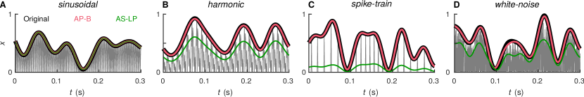
Figure 2: Typical examples of the test signals (gray), featuring nonstationary sinusoidal (A), harmonic (B), spike-train (C), and stationary white-noise (D) carriers, and their modulators obtained by using the AP-B (red) and AS-LP (green) algorithms. The signals are represented by their absolute values here. The predefined modulators are shown in black.

III-C AP-Projected

As argued above, the AP-A and AP-B algorithms produce modulator estimates that are expected to tightly follow the original $\mathbf{m}$ if the conditions analogous to those discussed in Section II-C are met. These estimates, however, do not always hold the minimum-norm property (6). A classical AP scheme that guarantees minimum-norm solutions is known under the name of Dykstra [44, 45]. In particular, Dykstra’s algorithm calculates the projection of a point in $\mathbb{R}^{n}$ onto the feasible set. Thus, by choosing an appropriate initial condition, the solution with a minimized norm can be obtained (see Proposition III.5 next and its proof in Suppl. Mat. F). We consider a version of this algorithm adapted to solve the demodulation problem and call it “AP-Projected” (AP-P).

  Algorithm: AP-Projected (AP-P)  

1:  Set: $N_{iter}$, $\epsilon_{tol}$

2:  Initialize: $i=0$, $\epsilon^{(0)}=\|\mathbf{s}\|_{2}/\sqrt{n}$, $\mathbf{m}^{(0)}=\mathbf{c}^{(0)}=|\mathbf{s}|$

3:  while $\epsilon^{(i)}>\epsilon_{tol}$ and $i<N_{iter}$ do

4:     $i=i+1$

5:     $\mathbf{a}^{(i)}=\mathbf{P}_{\mathcal{S}_{\varpi}}[\mathbf{m}^{(i-1)}]$

6:     $\mathbf{m}^{(i)}=\mathbf{P}_{\mathcal{S}_{\raisebox{1.0pt}{\scalebox{0.4}{$\geq|$}\scalebox{0.52}{$\mathbf{s}$}\scalebox{0.4}{$|$}}}}[\mathbf{a}^{(i)}-\mathbf{c}^{(i-1)}]$

7:     $\mathbf{c}^{(i)}=\mathbf{m}^{(i)}-(\mathbf{a}^{(i)}-\mathbf{c}^{(i-1)})$

8:     $\epsilon^{(i)}=\sqrt{(\|\mathbf{m}^{(i-1)}-\mathbf{a}^{(i)}\|_{2}^{2}+\|\mathbf{m}^{(i)}-\mathbf{a}^{(i)}\|_{2}^{2})/(2\cdot n)}$

9:  end while

10:  Finalize: $\mathbf{\hat{m}}=\mathbf{m}^{(i)}$  

Proposition III.5.

A sequence $\mathbf{m}^{(0)},\mathbf{m}^{(1)},\ldots,\mathbf{m}^{(i)},\ldots$ formed by the AP-P algorithm for $\epsilon_{tol}=0$ and $N_{iter}\to+\infty$ converges to a unique $\mathbf{m}^{\dagger}\in\mathcal{S}_{\raisebox{1.0pt}{\scalebox{0.5}{$\geq|$}\scalebox{0.72}{$\mathbf{s}$}\scalebox{0.5}{$|$}}}\cap\mathcal{S}_{\varpi}$ such that $\|\mathbf{m}^{\dagger}\|_{2}\leq\|\mathbf{x}\|_{2}$ for every $\mathbf{x}\in\mathcal{S}_{\raisebox{1.0pt}{\scalebox{0.5}{$\geq|$}\scalebox{0.72}{$\mathbf{s}$}\scalebox{0.5}{$|$}}}\cap\mathcal{S}_{\varpi}$. The convergence is monotonic, i.e., $\|\mathbf{m}^{(i+1)}-\mathbf{m}^{\dagger}\|_{2}\leq\|\mathbf{m}^{(i)}-\mathbf{m}^{\dagger}\|_{2}$ for $i\geq 0$.

The AP-P differs from the AP-B in that, before projecting a point onto $\mathcal{S}_{\raisebox{1.0pt}{\scalebox{0.5}{$\geq|$}\scalebox{0.72}{$\mathbf{s}$}\scalebox{0.5}{$|$}}}$, an increment produced by the projection onto this set in the previous iteration is subtracted. This correction may cause the infeasibility error $\|\mathbf{m}^{(i)}-\mathbf{a}^{(i)}\|_{2}/\sqrt{n}$ estimated after projecting onto $\mathcal{S}_{\raisebox{1.0pt}{\scalebox{0.5}{$\geq|$}\scalebox{0.72}{$\mathbf{s}$}\scalebox{0.5}{$|$}}}$ to drop to zero intermittently before the final solution is reached, making it an inappropriate option as the stopping criterion. Hence, in contrast to the AP-B and AP-A algorithms, we defined the $\epsilon$ for the AP-P as a combination of the infeasibility errors evaluated after projecting onto both sets $\mathcal{S}_{\varpi}$ and $\mathcal{S}_{\raisebox{1.0pt}{\scalebox{0.5}{$\geq|$}\scalebox{0.72}{$\mathbf{s}$}\scalebox{0.5}{$|$}}}$ at each iteration (see line 8 above). This error measure is strictly positive and converges to zero when $N_{iter}\to+\infty$ [46].

The understanding of the convergence rate of Dykstra’s scheme is limited. It was shown that the convergence is geometric for an intersection of half-spaces [47, 48]. Nevertheless, no equivalent result exists for other convex sets. Moreover, it was demonstrated that the convergence rate of this algorithm may depend on the initial conditions and may be considerably slower than that of AP algorithms based on pure projections [49].

III-D Computational complexity

Except for the projection operator $\mathbf{P}_{\mathcal{S}_{\varpi}}$, each iteration of the three formulated AP algorithms relies on vector addition, scalar product, and value update. These are linear in the number of sample points. The operator $\mathbf{P}_{\mathcal{S}_{\varpi}}$ can be easily implemented by using the direct and inverse fast Fourier transforms (FFTs) and setting the relevant elements of the signal to zero in the Fourier domain. The current state-of-the-art FFT algorithms have an $\mathcal{O}(n\log n)$ time complexity [50], which, thus, sets the overall time complexity of the AP algorithms introduced in this work. Our numerical experiments suggest that the convergence speed in terms of iteration number is independent of the signal length (see Suppl. Mat. M).

IV Performance Tests

To evaluate the AP algorithms introduced above, we compared their performance with the AS and LDC demodulation approaches when applied to infer the modulator of predefined synthetic test signals. The LDC approach was implemented by using two state-of-the-art quadratic programming solvers: Gurobi (v8.1.1) [51] and OSQP (v0.6.0) [52]. The AS demodulation was achieved by using the FFT-based approach [53]. In that case, we additionally low-pass filtered the obtained modulator estimate with $\mathbf{P}_{\mathcal{S}_{\varpi}}$ to regularize it. We refer to this modified demodulation scheme as AS-LP.

IV-A Test signals

The test signals were composed as products of a modulator and a carrier: $\mathbf{s}=\mathbf{m}\circ\mathbf{c}$. Four types of $\mathbf{c}$, approximating basic building blocks of real-world signals, were used: nonstationary sinusoidal, harmonic, and spike-train, as well as stationary white-noise (see, respectively, (176), (180), (184), and (188) in Suppl. Mat. I). The former two were combined with modulators of nonstationary Gaussian origin, while the latter two types of carriers were paired with the so-called maximally-uniformly distributed modulators (see, respectively, (160) – (162) and (163) – (168) in Suppl. Mat. I).

In all cases, modulator and carrier pairs were selected to meet the core recoverability condition $\lceil n/d\rceil\geq 2\varpi-1$, at least approximately. The remaining parameters of $\mathbf{m}$ and $\mathbf{c}$ (see Suppl. Mat. I) were chosen to imitate realistic conditions as much as possible. For example, in all cases, signals were taken as segments of longer time series, and thus, were not $n$-periodic. The center frequencies of the sinusoidal and harmonic carriers were set so that only sample points with $|c_{i}|\approx 1$ rather than $|c_{i}|=1$ were available.

IV-B Performance evaluation

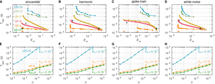
Figure 3: Performance evaluation. A–D: Pareto fronts in the $(E_{m},T_{\mathrm{cpu}})$ plane for different demodulation algorithms applied to the four different types of test signals when window splitting is used. Green stars mark the results of the AS-LP method. Color arrowheads point to the lower bounds on $E_{m}$ for the respective AP algorithms. Black arrowheads indicate demodulation error $E_{m}$ values of the AP-B algorithm calculated locally for signal windows shown in Fig. 2. E–H: Dependence of the demodulation time $T_{\mathrm{cpu}}$ on the signal length $n$ at $\epsilon_{tol}=10^{-3}$ when window splitting is not exploited. $E_{m}$ values in the legends correspond to demodulation results at $n=2^{14}\approx 1.6\cdot 10^{4}$.

Demodulation performance was evaluated by using two complementary measures: 1) error of the modulator estimate, $E_{m}=\|\mathbf{m}-\mathbf{\hat{m}}\|_{2}/\|\mathbf{m}\|_{2}$; and 2) execution time of the algorithm on the computer, $T_{\mathrm{cpu}}$. We evaluated the AP and LDC algorithms in the mode when $T_{\mathrm{cpu}}$ depends on the total number of sample points but not on the effective degrees of freedom. This choice made the results general, independent of a selected cutoff frequency $\varpi$. To insure against outliers, we averaged $E_{m}$ and $T_{\mathrm{cpu}}$ over ten independent signal realizations.

Execution of the AP and LDC algorithms is controlled by a set of metaparameters whose choice influences the output. Therefore, we aimed for the Pareto fronts, not separate points, in the $(E_{m},T_{\mathrm{cpu}})$ plane. Due to the computing speed limitations inherent to the LDC approach, we had to exploit signal decomposition into separate fragments for this analysis. In particular, signals were split into segments that were demodulated separately and then put together [19]. This allowed achieving a linear growth in the computation time with the total length of the signal, and hence, speeding up the calculations. After identifying the optimal control-parameter combinations, we compared all methods by demodulating whole signals.

Sets of the demodulation control parameters that we considered for the Pareto optimality analysis, including those defining the signal splitting, are provided in Suppl. Mat. J. Details on the execution of the performance tests on a computer can be found in Suppl. Mat. K.

IV-C Results

Fig. 2 shows representative fragments of the test signals from all four classes (gray) and their modulator estimates obtained by using the AS-LP (green) and AP-B (red) algorithms. Whereas the AP-B allows obtaining high-quality estimates $\mathbf{\hat{m}}$ in all four cases, the AS-LP does so only for sinusoidal signals.

Results of the performance evaluation in the form of Pareto fronts in the $(E_{m},T_{\mathrm{cpu}})$ plane for $n=2^{15}$ are displayed in Fig. 3 A–D. Panels E–H of the same figure show $T_{\mathrm{cpu}}$ vs. $n$ relations derived by using no window splitting. A closer analysis of these data reveals the following:

1. The AP algorithms feature lower bounds on the demodulation error $E_{m}$ than the LDC method (Fig. 3 A–D).

2. The AP algorithms are up to five orders of magnitude faster than their LDC counterparts for achieving the same $E_{m}$ when optimal signal window splitting is used (Fig. 3 A–D). The difference is even more pronounced when no window splitting is assumed (Fig. 3 E–H). For example, to process a 1 s length signal sampled at 16 kHz, the LDC needs $10^{4}$ s of CPU time, in contrast to $10^{-3}$ s taken by the AP-A.

3. $T_{\mathrm{cpu}}$ varies substantially (up to three orders of magnitude) even between different AP algorithms (Fig. 3 A–D). The AP-A ranks as the fastest, and the AP-P as the slowest one for all tested signals.

4. Despite the differences in $T_{\mathrm{cpu}}$, all AP algorithms feature similar lower bounds on $E_{m}$, except the spike-train signals, when the AP-B and AP-P can noticeably surpass the AP-A on the relative scale (Fig. 3 A–D). Nevertheless, on the absolute scale, the AP-A still performs reasonably well.

5. For all tested signals, the AP-A algorithm outperforms the AS-LP-based demodulation in the sense that it can achieve the same or smaller errors with the same $T_{\mathrm{cpu}}$ (Fig. 3 A–D). Moreover, compared with the AS-LP, AP algorithms exhibit much lower bounds on $E_{m}$.

6. Even without the window splitting (when the highest demodulation accuracy is attained), the AP-A algorithm takes only 2–3 times longer than the AS-LP method (Fig. 3 E–H).

We found that the decrease in $E_{m}$ along the Pareto fronts is mainly determined by the increase in the demodulation window size. In particular, the lower bounds on $E_{m}$ are achieved by the particular algorithms when the signal is demodulated using no window splitting. The relatively lower precision of the AP-A algorithm compared with AP-B and AP-P in the case of nonstationary spike-trains can be reduced to its acceleration mechanism. Indeed, in the AP-A, upscaling of iterates $\mathbf{a}^{(i)}$ is effectively based on the averaging of $(\mathbf{m}^{(i)}-\mathbf{a}^{(i)})$ over a window of length $\approx n/(2\pi\varpi)$ at each sample point. The precision of these estimates is more vulnerable to deviations from the exact recovery conditions for sparse carriers.

As can be expected, the high accuracy of modulator estimates achieved by the AP algorithms implies the high quality of carrier predictions $\mathbf{\hat{c}}=\mathbf{s}/\mathbf{\hat{m}}$ (see Suppl. Mat. L and Fig. 13 therein). The AP approach leaves the AS-LP behind in terms of carrier estimation for all four signal types considered (see Suppl. Mat. L). When applicable, the inferred $\mathbf{\hat{c}}$ can be further frequency-demodulated by using dedicated techniques (see [1, 54], and references given there).

The impressive performance of the AP-A algorithm in terms of $E_{m}$, $E_{c}$, and $T_{\mathrm{cpu}}$ makes it an ideal candidate for amplitude demodulation of a wide range of signals. Its AP-B and AP-P counterparts can be used instead if higher precision is needed in specific cases, as illustrated by the spike-train signals above.

V Convergence Tests

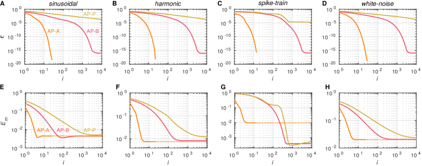
Figure 4: Convergence analysis of the AP algorithms. A–D: Dependence of the infeasibility error $\epsilon$ on the iteration number $i$ for the AP-B, AP-A, and AP-P algorithms applied to the four different types of test signals with $n=2^{15}$ and no window splitting. E–H: Analogous plots to A–D made for the demodulation error $E_{m}$ instead of $\epsilon$. Dotted lines show hypothetical $E_{m}$ values that would be obtained if we continued the AP-A iterations after reaching the final solution.

To clarify the differences between the $T_{\mathrm{cpu}}$ estimates of the three AP algorithms and understand the relationship between the demodulation and infeasibility errors, we performed a convergence analysis with the test signals from the previous section. The simulation results for fixed $n=2^{15}$ using no window splitting are summarized in Fig. 4. A closer inspection uncovers the following:

1. The convergence rates in terms of both $\epsilon$ and $E_{m}$ parallel the differences in the computing speed of different AP algorithms. Among them, the fastest is the AP-A, which reaches any given $\epsilon$ or $E_{m}$ level with the smallest num-ber of iterations. The AP-P algorithm is the slowest one.

2. The AP-A algorithm converges in a finite number of iterations ($<30$) for all types of test signals studied. In particular, it requires only $\leq 5$ iterations to reach the plateau level of the demodulation error $E_{m}$. This fact explains the extraordinary computational efficiency of the AP-A documented in Section IV.

3. Differently from the convergence error $\|\mathbf{m}^{(i)}-\mathbf{m}^{\dagger}\|_{2}/\sqrt{n}$, the dependence of $E_{m}^{\scalebox{0.7}{(}i\scalebox{0.7}{)}}$ on $i$ can be nonmonotonic if $\mathbf{m}^{\dagger}$ is not strictly equal to $\mathbf{m}$ (Fig. 4 E, G). Then, $E_{m}^{(i)}$ starts growing with increased $i$ after reaching the minimum point. However, this growth is mild and of no practical importance as long as $\mathbf{m}^{\dagger}\approx\mathbf{m}$, i.e., $\mathbf{\hat{m}}\approx\mathbf{m}$.

The results shown in Fig. 4 represent only signals of fixed length ($n=2^{15}$ sample points). Additional simulations suggested no dependence on $n$ (see Suppl. Mat. M).

VI Robustness Tests

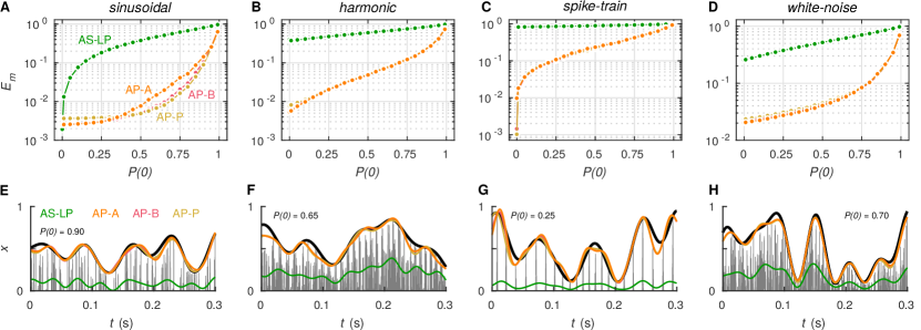
Figure 5: Robustness evaluation. A–D: Dependence of the demodulation error $E_{m}$ on $P(0)$ (the probability of missing points) for the four types of test signals and different AP algorithms at $\epsilon_{tol}=10^{-4}$ (color coding). E–H: Representative examples of demodulation at various $P(0)$ levels for the test signals from A–D. Color code: gray – the absolute-value signal, black – the original modulator, color – modulators inferred by different algorithms.

The pivotal condition for successfully separating the modulator-carrier information of a given signal by our approach is $\lceil n/d\rceil\geq 2\omega-1$. In practice, this requirement is not necessarily met. Hence, the choice of a particular demodulation method must be guided not only by the algorithmic efficiency but also robustness to deviations from the ideal recovery conditions. To shed light on this aspect, we considered demodulation of the test signals from Section IV-A corrupted by a multiplicative Bernoulli-$\{0,1\}$ noise. In this setup, sample points, including the decisive $|s_{i}|=m_{i}$, are eliminated with the probability of “0” elements in the noise ($P(0)$), effectively decreasing the value of $\lceil n/d\rceil$.

We found that all three AP algorithms considered in this work show a similar degree of robustness to increased $P(0)$ (see Fig. 5). Only in the case of sinusoidal signals, the AP-A is slightly inferior to the AP-B and AP-P. Interestingly, the advantage of the AP-B and AP-P over the AP-A in the case of spike-train signals discussed in Section IV-C disappears in the presence of even small distortions (see Fig. 5 C). The differences in the $E_{m}$ vs. $P(0)$ relations seen in Fig. 5 A–D are predetermined by different densities of $|c_{i}|\simeq 1$ points inherent to each carrier type. Analogous results to those shown in Fig. 5 A–D are obtained when considering carrier recovery via $\mathbf{\hat{c}}=\mathbf{s}/\mathbf{\hat{m}}$ (see Fig. 14 in Suppl. Mat. L).

In contrast to the AP approach, the AS-based demodulation is highly vulnerable to missing sample points, and hence, to decreased $\lceil n/d\rceil$ (Fig. 5 A–D). Even for sinusoidal signals, which the AS and AS-LP are specially designed for, the zeroing of data points leads to a rapid decline in demodulation quality (Fig. 5 A, E).

The robustness to missing sample points endows the AP demodulation method with a highly valuable practical advantage. In particular, it can be exploited in real-world situations when: 1) the sampling rate is low; 2) some segments of the signal values are lost; 3) some sample points are corrupted by noise such that the level of these points can be reduced below the real modulator by low-pass filtering or explicitly identifying them. In this context, the PAD and LDC demodulations compare to the AP approach by construction [23].

VII High-Level Properties

As emphasized in Section II, different demodulation methods can be derived by requesting adherence of the inferred modulators and carriers to a set of particular properties. Typically, various combinations that consist of a few out of many reasonable requirements are sufficient for unique demodulation formulations. However, some of these requirements are inconsistent with each other, making virtually all classical demodulation approaches fail to satisfy one or another essential condition [9, 25, 23]. For example, the AS demodulation method may return an unbounded modulator estimate for a bounded signal [25].

The AP approach formulated in this work is compatible with the following high-level requirements, which have crystallized as inseparable from the notion of proper amplitude demodulation with time [19], [23, Section 3.5.2]:

• Boundedness: The modulator and carrier of a bounded signal are bounded. In particular, it is required that $-\infty<\hat{m}_{i}<+\infty$ and $-1\leq\hat{c}_{i}\leq 1$ for every $i\in\mathcal{I}_{n}$. In the case of the AP approach, the boundedness of the modulator is guaranteed by the convergence of the AP algorithms. The boundedness of the carrier then follows from the constraint $\hat{m}_{i}\geq|s_{i}|$ and the fact that $\mathbf{\hat{c}}=\mathbf{s}\circ\mathbf{\hat{m}}^{-1}$.

• Scale covariance: The modulator and carrier of a scaled signal are equal to the modulator and carrier obtained from the original signal and then scaled by the same amount. The adherence of the AP approach to this condition follows from two facts. First, projection operators $\mathbf{P}_{\mathcal{S}_{\raisebox{1.0pt}{\scalebox{0.4}{$\geq|$}\scalebox{0.52}{$\mathbf{s}$}\scalebox{0.4}{$|$}}}}$ and $\mathbf{P}_{\mathcal{S}_{\varpi}}$ are homogeneous with degree 1, i.e., $\mathbf{P}_{\mathcal{S}}[\alpha\cdot\mathbf{s}]=\alpha\cdot\mathbf{P}_{\mathcal{S}}[\mathbf{s}]$. Second, each iteration of the AP algorithms can be expressed as a weighted sum of these projections with the weights independent of the scale.

• Smoothness: The modulator of a bounded signal in its continuous-time representation is smooth. Because we use a discrete-time representation, this requirement has to be adjusted. In particular, let us denote by $\hat{m}^{\prime}_{t}$ and $\hat{m}^{\prime}_{t+\Delta t}$ the finite-difference approximations of the modulator’s time-derivatives of any order at two subsequent time points: $t$ and $t+\Delta t$. Then, we require that, for any $\epsilon>0$, there exists a $\delta>0$ such that $|\hat{m}^{\prime}_{t+\Delta t}-\hat{m}^{\prime}_{t}|<\epsilon$ when $|\Delta t|<\delta$. The AP approach satisfies this requirement through the boundedness of the modulator and the bandwidth constraint set by $\mathcal{S}_{\varpi}$ on it.

• Idempotence: Information associated with the qualities of modulators and carriers is fully separated. Specifically, demodulation reapplied to an estimated modulator (carrier) must return the same modulator (carrier). The AP approach satisfies the idempotence requirement for the modulator exactly. Indeed, when any AP algorithm is applied to its final solution $\mathbf{\hat{m}}=\mathbf{m}^{\dagger}$, the latter is recognized as the final solution again after the first new iteration by construction. Regarding the carrier, the idempotence holds whenever the recovery conditions discussed in Section II-C are met. That is because, in those cases, $\mathbf{\hat{c}}$ resulting from the first demodulation contains a sufficient number of $|\hat{c}_{i}|=1$ points to uniquely define the $\mathbf{\hat{m}}=\mathbf{1}$ as the norm-minimizing element of $\mathcal{S}_{\raisebox{1.0pt}{\raisebox{0.65pt}{\scalebox{0.58}{$\geq|$}}\scalebox{0.72}{$\mathbf{\hat{c}}$}\raisebox{0.65pt}{\scalebox{0.58}{$|$}}}}\cap\mathcal{S}_{\varpi}$. If the recovery conditions are met only approximately, we expect no marked deviations from the idempotence condition (see Fig. 16 in Suppl. Mat. N).

By fulfilling the above requirements, the AP approach parallels the methods of PAD and LDC demodulation [23, 19]. In this sense, all of them outperform the classical techniques.

VIII Demodulation of Speech Signals

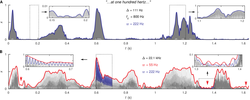
Figure 6: Direct demodulation of speech signals. A: A band-pass-filtered signal of an utterance “…at one hundred hertz …” by a female speaker; the signal was obtained with an equivalent rectangular bandwidth filter of the cochlea centered at $f_{c}=800~{}\mathrm{Hz}$ and $\Delta=111~{}\mathrm{Hz}$. B: The original signal of the utterance used in panel A (full bandwidth of $22.1~{}\mathrm{kHz}$). In both panels, gray color marks the absolute-value version of the signals considered for demodulation. Blue and red lines show their modulators obtained by using the AP-A algorithm with the cutoff frequency $\omega$ set to, respectively, $55~{}\mathrm{Hz}$ and $222~{}\mathrm{Hz}$. Insets display time-expanded segments of the original window. Red arrowheads indicate the ringing artifacts of the modulator at some prolonged intervals of low signal levels. Source of the original signal: audio edition of The Economist magazine, issue March 19th 2016, article “Restoring lost memories.”

Amplitude demodulation is of central importance in various tasks of processing and analysis of speech signals. Application-wise, this procedure is used in hearing restoration [10, 55], speech recognition [2, 56, 57], and source separation [58, 59]. On the theory side, amplitude demodulation is exploited in neurophysiological and psychophysical studies of auditory information processing in the brain [11, 60, 61, 12]. Depending on the problem, demodulation of either narrow subband [58, 56], intermediate subband [11, 10], or whole wideband signal [62, 12] is needed. In all these cases, modulators and carriers convey the information about specific aspects of speech, e.g., semantic meaning, associated emotion, or speaker identity, that need to be extracted.

In this section, we apply the newly-introduced AP approach to speech demodulation to further demonstrate its potential. To represent the range of possible real-world situations, we consider two limiting signal types: 1) a narrow subband component of a signal obtained by a standard auditory ERB filter [63]; and 2) the original wideband signal.

VIII-A Direct demodulation

By construction, the output of auditory ERB filters occupies a frequency subband whose width $\Delta$ is much smaller than its center frequency $f_{c}$ [63]. The resulting signal is an amplitude- and phase-modulated sinusoidal $\mathbf{s}=\mathbf{m}\circ\sin(2\pi f_{c}\mathbf{t}+\bm{\varphi})$, with most of the energies of $\mathbf{m}$ and $\bm{\varphi}$ residing in the frequency interval $[0,\Delta]$ [64]. Hence, by the recovery conditions of the AP approach (see Section II-C), setting the cutoff frequency $\varpi$ between $\Delta$ and $f_{c}$ necessarily results in accurate estimates $\mathbf{\hat{m}}$ and $\mathbf{\hat{c}}$. In particular, note that the local maximums of $|\mathbf{s}|$ correspond to the true sample points $|s_{i}|=m_{i}$. Thus, the high quality of demodulation is visually conveyed by a tight match of $\mathbf{\hat{m}}$ and $|\mathbf{s}|$ at these sample points. We illustrate our claims in Fig. 6 A, where a band-pass component of a female utterance “…at one hundred hertz …” with $f_{c}=800\,\mathrm{Hz}$, $\Delta=111\,\mathrm{Hz}$, and $\varpi=222\,\mathrm{Hz}$ is considered. Taking into account that the local maximum points $|s_{i}|$ are locally regular and that they correspond to $m_{i}$, we could exploit Proposition A.2 in Suppl. Mat. A to find that $E_{m}\leq 8\cdot 10^{-3}$.

Wideband speech signals are more challenging than their narrow subbands. They are built of temporarily structured segments of quasi-random and quasi-harmonic carriers, possibly featuring frequency glides [65]. These carriers are amplitude-modulated at different timescales, ranging between a hundred milliseconds and several seconds [23, 66]. The power spectral density of the corresponding modulators is vanishingly small above 20 Hz (see Fig. 1 in [67]). Moreover, as we demonstrate in Suppl. Mat. O, the carrier components of natural speech signals align to the recoverability conditions of the AP approach for $\mathbf{m}\in\mathcal{M}_{\omega}$ with $\omega$ up to at least $\sim 50\,\mathrm{Hz}$. Therefore, we expect appropriate performance from the AP algorithms in the setting of wideband speech.

Fig. 6 B displays demodulation results of the full-band version of the speech segment considered in Fig. 6 A by the AP-A algorithm with $\varpi=55~{}\mathrm{Hz}$. The obtained $\mathbf{\hat{m}}$ (red) envelops separate phonemes of the sound waveform tightly, indicating appropriate recovery of the true $\mathbf{m}$ (see Section VIII-B next). However, intervals corresponding to prolonged transitions between phonemes or words are corrupted by ringing artifacts (marked by red arrowheads in Fig. 6 B), implying the necessity of higher frequency components to represent these transitions. Hence, although the power spectral density of the true $\mathbf{m}$ is very low above $20\,\mathrm{Hz}$, it sums to a noticeable contribution. Unfortunately, any attempt to cancel the artifacts by just increasing $\varpi$ fails by breaking the recovery conditions, as illustrated by the blue line in Fig. 6 B ($\varpi=222~{}\mathrm{Hz}$ there). No improvement is achieved by utilizing the AP-B, AP-P, or LDC algorithms either (data not shown).

VIII-B Demodulation using dynamic range compression

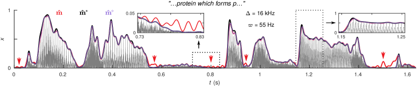
Figure 7: Demodulation of speech signals using dynamic range compression. An audio signal of “…protein which forms p …” uttered by a female speaker (full bandwidth of $16~{}\mathrm{kHz}$). Gray – the absolute-value version of the signal considered for demodulation, red – its modulator obtained by using the AP-A algorithm with $\omega=55~{}\mathrm{Hz}$ and no compression (as in Fig. 6), black – modulator of the signal obtained when employing the dynamic range compression [see (13)], violet – interpolation of the latter two [see (14)]. Red arrowheads indicate ringing artifacts of the modulator estimate. Source of the original signal: the same as Fig. 6.

The aforementioned problem with modulator estimates of signals with sharp transitions to/from prolonged intervals of low-signal amplitude can be resolved by using a dynamic range compression. In particular, instead of demodulating the original signal $\mathbf{s}$ directly, we first apply a chosen AP algorithm to its compressed version:

$$\mathbf{\underline{s}}=\mathrm{sgn}(\mathbf{s})\circ\mathbf{|s|}^{1/p}.$$ (12)

Here, $p\in(1,+\infty)$ controls the level of compression. The modulator estimate $\mathbf{\hat{m}^{*}}$ of $\mathbf{s}$ is then evaluated by inverse-transforming the modulator $\mathbf{\underline{\hat{m}}}$ of $\mathbf{\underline{s}}$:

$$\mathbf{\hat{m}^{*}}=\mathbf{\underline{\hat{m}}}^{p}.$$ (13)

The idea behind (12) is that the compression makes signals more uniform and, effectively, smooths their sharp changes responsible for ringing artifacts in the modulator estimates. These sharp changes are restored in the modulators without artifacts by the inverse transform (13).

The expected effect of the compression procedure is illustrated in Fig. 7, where signal demodulation of an utterance “…protein which forms p…” is considered. Differently from the direct demodulation result $\mathbf{\hat{m}}$ (red line), the estimate $\mathbf{\hat{m}^{*}}$ obtained by using the compression with $p=3$ (black line) shows good alignment with $|\mathbf{s}|$ in the segments of both low and high intensity. To justify that this alignment really reflects the recovery of the true modulator, we performed additional tests where chimeric signals built of $\mathbf{\hat{m}^{*}}$ from Fig. 7 and natural speech carriers were demodulated (see Suppl. Mat. O). We found low demodulation errors, with $E_{m}$ ranging between $9\cdot 10^{-3}$ and $5\cdot 10^{-2}$ for different carrier components of speech signals (see Fig. 18).

The compression level $p=3$ used above was adjusted by a trial and error for speech signals. In general, the gains in accuracy at low levels with increased $p$ comes at the expense of reduced precision of modulator estimated at high signal levels. Thus, a compromise between those two effects must be reached to find an optimal $p$. Moreover, the precision of the modulator estimates can be further increased by interpolating between $\mathbf{\hat{m}^{*}}$ (more accurate for low signal levels) and $\mathbf{\hat{m}}$ (more accurate for high signal levels). For example, the violet line in Fig. 7 shows a weighted average of the form

$$\mathbf{\hat{m}^{\diamond}}=\mathbf{\hat{m}}\circ\mathbf{w}+\mathbf{\hat{m}^{*}}\circ(1-\mathbf{w}),$$ (14)

where

$$\mathrm{w_{i}}=\bigg{(}\frac{1-e^{a\cdot(\mathrm{\hat{m}^{*}_{i}}/\max[\mathbf{\hat{m}^{*}}])}}{1+e^{a\cdot(\mathrm{\hat{m}^{*}_{i}}/\max[\mathbf{\hat{m}^{*}}])-b}}\bigg{)}\cdot\bigg{(}\frac{1-e^{a}}{1+e^{a-b}}\bigg{)}^{-1}$$ (15)

for $i\in\mathcal{I}_{n}$, with $b=3$ and $a=10$. In general, an optimal interpolation between $\mathbf{\hat{m}}$ and $\mathbf{\hat{m}^{*}}$ can be learned by minimizing $\|\mathbf{\hat{m}^{\diamond}}\|_{2}^{2}$ over a chosen class of functions. Other compression models than (12), e.g., $\mathbf{\underline{s}}=\mathrm{sgn}(\mathbf{s})\circ\log(1+p\cdot|\mathbf{s}|)$, can be used to evaluate $\mathbf{\hat{m}^{*}}$ as well.

VIII-C Demodulation in real-time

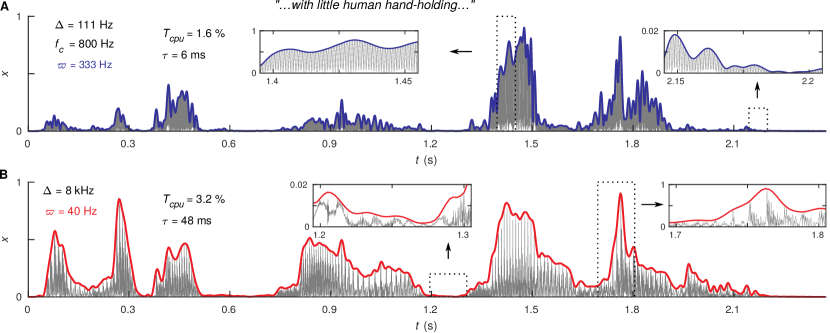
Figure 8: Demodulation in real-time. A: A band-pass-filtered signal of an utterance “…with little human hand-holding …” by a male speaker; the signal was obtained with an equivalent rectangular bandwidth filter of the cochlea centered at $800\,\mathrm{Hz}$ (bandwidth of $111~{}\mathrm{Hz}$). B: The original signal of the utterance used in panel A (full bandwidth of $8~{}\mathrm{kHz}$). In both panels, gray color marks the absolute-value version of the signals considered for demodulation. Blue and red lines show their modulators obtained by using the real-time version of the AP-A algorithm with the cutoff frequency $\omega$ set to, respectively, $333~{}\mathrm{Hz}$ and $40~{}\mathrm{Hz}$. Source of the original signal: audio edition of The Economist magazine, issue March 19th 2016, article “Artificial intelligence and Go.”

A number of amplitude demodulation applications, e.g., speech recognition [2], ultrasound imaging [68], and cochlear prosthesis [55], necessitate real-time processing. As we demonstrate below, the exceptional computational efficiency of the AP approach allows it to fulfill that requirement.

The nature of the task implies that online modulator estimates have to be generated by sequentially demodulating windowed segments $\mathbf{s}^{(j)}$ of a signal $\mathbf{s}$ at each updated sample point $j$ across time:

$$\mathbf{s}^{(j)}:s_{i}^{(j)}=w_{i}\cdot s_{j-k_{l}-1+i},\qquad i\in\{1,2,\ldots,k\}.$$ (16)

Here, $k$ is the number of sample points corresponding to the segment, and $k_{l}$ denotes the number of sample points of it that are to the left of the current point $j$. $w_{i},w_{2},\ldots,w_{k}$ are vector elements of the window function. The real-time modulator estimate $\hat{m}_{j}^{\star}$ at sample point $j$ is calculated as

$$\hat{m}_{j}^{\star}=\hat{m}_{k_{l}+1}^{(j)},$$ (17)

where $\mathbf{\hat{m}}^{(j)}$ is a modulator estimate of $\mathbf{s}^{(j)}$.

It follows from the time-frequency uncertainty principle [8] that accurate evaluation of $\hat{m}_{j}^{\star}$ requires $\mathbf{s}^{(j)}$ with a duration of the order of the inverse of the effective bandwidth of the modulator, or longer. This condition sets the lower bounds on the segment length $k$ and sampling delay $k_{\tau}=k-k_{l}-1$ of $\mathbf{\hat{m}}^{\star}$. We found empirically that $k_{\tau}\approx 2\cdot(f_{s}/\varpi)$ and $k\approx 4\cdot(f_{s}/\varpi)$ are typically sufficient for accurate demodulation of wideband speech. These numbers are around two times smaller for narrow frequency band components of these signals. We know that $\varpi\geq 40~{}\mathrm{Hz}$ for the wideband speech and its subbands. Thus, delays $k_{\tau}\leq 50~{}\mathrm{ms}$ for estimating $\mathbf{\hat{m}}^{\star}$ are sufficient without a sacrifice in precision then. The main requirement for the window function in (16) is that it smoothly scales the signal to 0 at the boundaries, with no effect at the midst. We used a modified version of the Hann window for this purpose:

$$w_{i}=\begin{cases}\sin^{2}\Big{(}\frac{\pi\cdot(i-1)}{2\cdot k_{l}}\Big{)},&\mbox{$\quad 1\leq i\leq k_{l}$}\\ 1,&\mbox{$\quad i=k_{l}+1$}\\ \cos^{2}\Big{(}\frac{\pi\cdot(i-k+k_{\tau})}{2\cdot k_{\tau}}\Big{)},&\mbox{$\quad k-k_{\tau}+1\leq i\leq k$}\end{cases}.$$ (18)

Fig. 8 shows simulation results of real-time demodulation of a male utterance “…with little human hand-holding …” (sampling rate $f_{s}=16~{}\mathrm{kHz}$) based on the AP-A algorithm. There, demodulation was performed with $k=1536$ and $k_{\tau}=768$ ($\tau=48~{}\mathrm{ms}$) for the original signal (Fig. 8 B). Its subband component centered at 800 Hz (Fig. 8 A) was processed with $k=128$ and $k_{\tau}=65$ ($\tau=4~{}\mathrm{ms}$). In each case, $\hat{m}^{\star}_{j}$ was updated with the frequency of $10\cdot\varpi$. The obtained estimates $\mathbf{\hat{m}^{\star}}$ are in very good agreement with $\mathbf{\hat{m}^{*}}$ derived by using offline demodulation of the whole signal, with $\|\mathbf{\hat{m}^{\star}}-\mathbf{\hat{m}^{\diamond}}\|_{2}/\|\mathbf{\hat{m}^{\diamond}}\|_{2}<0.02$. Importantly, they were achieved with modest CPU usage: $T_{\mathrm{cpu}}$ amounted to only 1.6 % (subband signal) and 3.2 % (wideband signal) of the time length of the demodulated signal on an Intel Core i7-7700 CPU run in single-thread mode. For comparison, these numbers were, respectively, $\sim 5\cdot 10^{3}$ and $\sim 6\cdot 10^{4}$ times higher for the LDC method.

An advantageous side effect of splitting the signal into small windows for demodulation is that it prevents the ringing artifacts (compare Fig. 8 B and Fig. 6 B). This is so because signal levels do not typically spread over different scales in a short time window. The window splitting also allows generalizing demodulation to situations when the cutoff frequency $\omega$ of the modulator varies strongly in time.

IX Extensions and Generalizations

IX-A Demodulation in higher dimensions

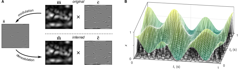
Figure 9: Demodulation in 2D by using the AP-A algorithm. A: Synthetic fringe pattern of moderate bandwidth. Left – the pattern to demodulate, upper right – the original modulator and carrier, lower right – the inferred modulator and carrier. B: Wideband signal consisting of randomly-placed spikes of finite width. Black grid – the signal $\mathbf{\bar{s}}$ to demodulate, white grid – the original modulator $\mathbf{\overline{m}}$ of the signal, color surface – the estimated modulator.

Amplitude demodulation has found successful applications beyond the setting of 1D signals. Several 2D extensions of the classical AS approach have been introduced and used for solving tasks in computer vision [69, 7], analysis of speech spectrograms [70], and biomedical imaging [71, 4, 72]. The AS framework has also been extended to calculate modulators and carriers for signals over graphs [73]. These methods are limited to locally narrowband signals, which manifest visually as fringe patterns (see Fig. 9 A). This bandwidth restriction is evaded by a generalization of the AP approach to higher dimensions that we present next. The extension is immediate and follows from intuitive abstractions of the constraint sets introduced in Section II.

Consider a $D$-dimensional signal $s(t_{1},t_{2},\ldots,t_{D})$. Its uniformly sampled version $\mathbf{\overline{s}}$ is an element of an $n$-dimensional Euclidean space $\mathbb{T}^{n}_{D}$ of real-valued order $D$ tensors with $n=\prod_{i=1}^{D}n_{i}$ and the inner product $\langle\mathbf{\overline{s}}^{(1)},\mathbf{\overline{s}}^{(2)}\rangle=\sum_{i_{1}=1}^{n_{1}}\cdots\sum_{i_{D}=1}^{n_{D}}(\bar{s}^{(1)}_{i_{1}\cdots i_{D}}\cdot\bar{s}^{(2)}_{i_{1}\cdots i_{D}})$. The respective $D$-dimensional DFT is given by

$$\mathbf{\overline{F}}=\mathbf{F}^{(1)}\otimes\mathbf{F}^{(2)}\otimes\cdots\otimes\mathbf{F}^{(D)},$$ (19)

where $\mathbf{F}^{(i)}$ is a unitary DFT defined over $\mathbb{R}^{n_{i}}$. Then, the analogs of the constraint sets $\mathcal{S}_{\raisebox{0.9pt}{\scalebox{0.5}{$\geq$}\raisebox{-0.95pt}{\scalebox{0.65}{$\mathbf{0}$}}}}$, $\mathcal{S}_{\omega}$, $\mathcal{S}_{\raisebox{1.0pt}{\scalebox{0.5}{$\geq|$}\scalebox{0.72}{$\mathbf{s}$}\scalebox{0.5}{$|$}}}$, $\mathcal{S}_{\raisebox{1.0pt}{\scalebox{0.5}{$|..|\leq$}}\scalebox{0.67}{$\mathbf{1}$}}$, and $\mathcal{S}_{\raisebox{1.0pt}{\scalebox{0.45}{\{}}\raisebox{0.27pt}{\scalebox{0.55}{1}}\raisebox{1.0pt}{\scalebox{0.45}{\}}},d}$ from Section II read as

$$\mathcal{S}_{\raisebox{0.9pt}{\scalebox{0.5}{$\geq$}\raisebox{-0.95pt}{\scalebox{0.61}{$\mathbf{\bar{0}}$}}}} =\{\mathbf{\overline{x}}\in\mathbb{T}^{n}_{D}:\overline{x}_{i_{1}\cdots i_{D}}\geq 0,\,i_{j}\in\mathcal{I}_{n_{j}}\},$$

$$\mathcal{S}_{\scalebox{0.67}{$\bm{\omega}$}} =\{\mathbf{\overline{x}}\in\mathbb{T}^{n}_{D}:(\mathbf{\overline{F}}\hskip 1.0pt\mathbf{\overline{x}})_{i_{1}\cdots i_{D}}=0,\,i_{j}\in(\mathcal{I}_{n_{j}}\setminus\mathcal{I}_{n_{j}}^{\omega_{j}})\},$$ (20)

$$\mathcal{S}_{\raisebox{1.0pt}{\scalebox{0.5}{$\geq|$}\raisebox{-0.5pt}{\scalebox{0.72}{$\mathbf{\bar{s}}$}}\scalebox{0.5}{$|$}}} =\{\mathbf{\overline{x}}\in\mathbb{T}^{n}_{D}:\overline{x}_{i_{1}\cdots i_{D}}\geq|\bar{s}_{i_{1}\cdots i_{D}}|,\,i_{j}\in\mathcal{I}_{n_{j}}\},$$

and

$$\mathcal{S}_{\raisebox{1.0pt}{\scalebox{0.5}{$|..|\leq$}}\scalebox{0.67}{$\mathbf{\bar{1}}$}} =\{\mathbf{\overline{x}}\in\mathbb{T}^{n}_{D}:|x_{i_{1}\cdots i_{D}}|\leq 1,\,i_{j}\in\mathcal{I}_{n_{j}}\},$$ (21)

$$\mathcal{S}_{\raisebox{1.0pt}{\scalebox{0.45}{\{}}\raisebox{0.27pt}{\scalebox{0.55}{1}}\raisebox{1.0pt}{\scalebox{0.45}{\}}},\scalebox{0.7}{$\mathbf{d}$}} =\big{\{}\mathbf{\overline{x}}\in\mathbb{T}^{n}_{D}:(\forall i_{1}\cdot\cdot\cdot i_{D})R(i_{1}\cdot\cdot\cdot i_{D},\mathbf{\overline{x}},\mathbf{d})\geq 1,$$

$$\hskip 60.0pt(\exists i_{1}\cdot\cdot\cdot i_{D})R(i_{1}\cdot\cdot\cdot i_{D},\mathbf{\overline{x}},\mathbf{d})=1\},$$

where

$$\textstyle R(i_{1}\cdot\cdot\cdot i_{D},\mathbf{\overline{x}},\mathbf{d})=\textstyle\sum_{j_{1}\geq i_{1}}\cdot\cdot\cdot\sum_{j_{D}\geq i_{D}}\big{[}I_{\{1\}}(|\overline{x}_{j_{1}\cdots j_{D}}|)$$ (22)

$$\textstyle\cdot\theta\big{(}1-\sum_{k=1}^{D}(i_{k}-j_{k})^{2}/d_{k}^{2}\big{)}\big{]}-I_{\{1\}}(|\overline{x}_{i_{1}\cdots i_{D}}|).$$

Simply substituting (20) – (21) for their $D=1$ versions in (2), (4), (6), (8), (9), and (10) generalizes the modulator $\mathcal{M}_{\omega}$ and carrier $\mathcal{C}_{d}$ sets as well as the modulator estimator $\mathbf{\hat{m}}$ and the respective AP algorithms. In particular, an $\mathbf{\overline{m}}\in\mathcal{M}_{\bm{\omega}}$ is a nonnegative signal with a low-pass rectangular spectrum set by $\bm{\omega}=(\omega_{1},\ldots,\omega_{D})$ along each of the $D$ dimensions in the DFT domain. A $\mathbf{\overline{c}}\in\mathcal{C}_{\mathbf{d}}$ is a signal bounded between $-1$ and $1$ with the $|\bar{c}_{i_{1}\cdots i_{D}}|=1$ sample points packed sufficiently densely, as implied by $\mathbf{d}=(d_{1},\dots,d_{D})$.

Without providing formal proofs, we state that all propositions and assertions of Sections II and III about the modulator recoverability and convergence of the AP algorithms generalize to $D$-dimensional signals defined above. All quantitative conditions involving the parameters $\varpi$, $\omega$, $d$, $n$, and $n_{s}$ in the $D=1$ case are then replaced by elementwise conditions for $\varpi_{i}$, $\omega_{i}$, $d_{i}$, $n_{i}$, and $n_{s,i}$ at $i\in\mathcal{I}_{D}$.

Fig. 9 illustrates the potential of the AP-A algorithm with the help of two $D=2$ cases. Fig. 9 A shows successful demodulation results for a synthetic narrowband fringe pattern ($E_{m}=1\cdot 10^{-2}$, $E_{c}=3\cdot 10^{-2}$). Fig. 9 B displays high-accuracy demodulation of a wideband signal built of randomly-placed spikes of finite width as $\mathbf{\overline{c}}$ and a Gaussian random field with a rectangular amplitude spectrum as $\mathbf{\overline{m}}$. There, the white grid corresponds to the original $\mathbf{\overline{m}}$, while the color surface represents its estimate $\mathbf{\hat{\overline{m}}}$ ($E_{m}=4\cdot 10^{-3}$, $E_{c}=1\cdot 10^{-2}$).

The ability of the AP approach to deal with wideband signals allows it to cover a wider range of practically relevant situations. Among examples are nonlinear ultrasound imaging [4, 14], speech processing [20, 70], and complicated cases of optical interference/diffraction setups [74]. Moreover, it can also be of great use in time-critical imaging settings by providing high modulator estimation accuracy at low sampling rates of the signal (see, e.g., [72, 75]).

The minimum number of sample points necessary to cover simultaneously for appropriate demodulation increases exponentially with $D$. Therefore, the computational advantage of the AP over the PAD and LDC demodulation approaches is even more pronounced in higher dimensions. In fact, if evaluated by using the FFT method, $\overline{\mathbf{F}}$ features an $\mathcal{O}\big{(}n\log n\big{)}$ computational time complexity. Hence, the time complexity of the AP algorithms is defined by the total number of sample points of the signal irrespective of its dimensionality.

IX-B Generalized modulators and nonuniform sampling

The demodulation approach formulated in the present work builds on the assumption that modulators are nonnegative elements of a low-pass DFT subspace of $\mathbb{T}^{n}_{D}$. However, as follows from the convergence proofs in Suppl. Mat. F, all of the introduced AP algorithms are bound to converge to an $\mathbf{\hat{m}}\in\mathcal{M}_{\bm{\omega}}$ and a $\mathbf{\hat{c}}\in\mathcal{C}_{\mathbf{d}}$ independent of the origin of the linear subspace behind $\mathcal{M}_{\bm{\omega}}$. This naturally raises the question of whether the AP algorithms could recover true $\mathbf{m}$ and $\mathbf{c}$ under the generalized subspace assumption. Our preliminary experiments suggest a positive answer but subject to extra recovery conditions specific to a subspace of choice.

For example, consider a subset of $2\omega-1$ randomly chosen basis vectors of the DFT over $\mathbb{R}^{n}$. Denote the corresponding space as $\mathcal{F}_{\omega}$. It can be shown by example that a system resulting from random subsampling of the aforementioned vectors at $2\omega-1$ time points may be linearly dependent. If so, it then follows from the proof of Proposition 3 that, in contrast to an $\mathbf{m}\in\mathcal{S}_{\omega}$, full recovery of an $\mathbf{m}\in\mathcal{F}_{\omega}$ necessitates more than $2\omega-1$ true sample points.

The problem of formulating modulator recovery conditions for different linear subspaces sets directions for future studies. If successful, these extensions would allow to:

1. broaden the concept of the amplitude modulator beyond the low-pass DFT signals,

2. loosen the constraints on the positioning of the $|c_{i}|=1$ sample points for recoverable carriers whenever a more compact representation of modulators is available,

3. encompass nonuniform sampling.

While the above points are yet to be developed, the results of the present work already provide a strategy for an arbitrarily-accurate nonuniform sampling. Indeed, for any time grid $\mathbf{\tilde{t}}\in\mathbb{R}^{\tilde{n}}$, we can find a uniform grid $\mathbf{t}\in\mathbb{R}^{n}$ such that, for every $j\in\mathcal{I}_{\tilde{n}}$, there exists an $i\in\mathcal{I}_{n}$ with $|\tilde{t}_{j}-t_{i}|$ being arbitrarily small. We can then interpolate the original data $\mathbf{\tilde{s}}\in\mathbb{R}^{\tilde{n}}$ on the uniform grid $\mathbf{t}$ by

$$s_{i}=\begin{cases}\tilde{s}_{j},&\mbox{if $|\tilde{t}_{j}-t_{i}|=\min[|\tilde{t}_{j}\cdot\mathbf{1}-\mathbf{t}|]$}\\ 0,&\mbox{otherwise}\end{cases},\quad~{}i\in\mathcal{I}_{n},$$ (23)

to obtain an $\mathbf{s}\in\mathbb{R}^{n}$. The bandwidth constraint on $\mathbf{m}$ implies that all components of $\mathbf{s}$ corresponding to the true sample points of $\mathbf{\tilde{s}}$ are desirably close to the true sample points of the original signal if $n$ is large enough. Then, Proposition II.2 assures that modulator-carrier recovery is possible via (6) under the conditions discussed in Section II-C for uniformly sampled signals. The described strategy requires increasing the effective dimensionality of the signal. However, this may still be more efficient than evaluating metric projections onto subspaces spanned by arbitrary nonuniform sampling basis vectors, which are not orthogonal in general.

X Conclusion

In this paper, we have introduced a new approach to amplitude demodulation of arbitrary-bandwidth signals. We framed demodulation as a problem of modulator recovery from an unlabeled mix of its true and corrupted sample points. Taking this view, we showed that high-accuracy demodulation can be achieved via exact or approximate norm minimization of the modulator for a wide range of relevant signals. We formulated tailor-made alternating projection algorithms to achieve that in practice and tested them in a series of numerical experiments.

The generality and numerical efficiency of the new approach make it a preferred choice in many situations. In the context of narrowband signals, the new method outperforms the classical algorithms in terms of robustness to data distortions and compatibility with nonuniform sampling. When considering the demodulation of wideband signals, it surpasses the current state-of-the-art techniques in terms of computational efficiency by up to many orders of magnitude. Such performance enables practical applications of amplitude demodulation in previously inaccessible settings. Specifically, online and large-scale offline demodulation of wideband signals, signals in higher dimensions, and poorly-sampled signals become practically feasible. The algorithms underlying the new approach are simple and easy to implement on a computer.

References

- [1] D. Vakman, Signals, oscillations, and waves: A modern approach. Artech House, 1998.
- [2] B. E. D. Kingsbury, N. Morgan, and S. Greenberg, “Robust speech recognition using the modulation spectrogram,” Speech Commun., vol. 25, pp. 117–132, 1998.
- [3] M. G. Ruppert, D. M. Harcombe, M. R. P. Ragazzon, S. O. R. Moheimani, and A. J. Fleming, “A review of demodulation techniques for amplitude-modulation atomic force microscopy,” Beilstein J. Nanotechnol., vol. 8, pp. 1407–1426, 2017.
- [4] C. Wachinger, T. Klein, and N. Navab, “The 2D analytic signal for envelope detection and feature extraction on ultrasound images,” Medical Image Analysis, vol. 16, pp. 1073–1084, 2012.
- [5] P. Y. Ktonas and N. Papp, “Instantaneous envelope and phase extraction from real signals: Theory, implementation, and an application to EEG analysis,” Elsevier Signal Process., vol. 2, pp. 373–385, 1980.
- [6] M. T. Taner, F. Koehler, and R. E. Sheriff, “Complex seismic trace analysis,” Geophysics, vol. 44, pp. 1041–1063, 1979.
- [7] K. G. Larkin, D. J. Bone, and M. A. Oldfield, “Natural demodulation of two-dimensional fringe patterns. I.” J. Opt. Soc. Am. A, vol. 18, pp. 1862–1870, 2001.
- [8] D. Gabor, “Theory of communication. Part 1: The analysis of information,” J. Inst. Elec. Eng. Part III, vol. 93, pp. 429–441, 1946.
- [9] D. Vakman, “On the analytic signal, the Teager-Kaiser energy algorithm, and other methods for defining amplitude and frequency,” IEEE Trans. Signal Process., vol. 44, pp. 791–797, 1996.
- [10] B. S. Wilson, C. C. Finley, D. T. Lawson, R. D. Wolford, D. K. Eddington, and W. M. Rabinowitz, “Better speech recognition with cochlear implants,” Nature, vol. 352, pp. 236–238, 1991.
- [11] Z. M. Smith, B. Delgutte, and A. J. Oxenham, “Chimaeric sounds reveal dichotomies in auditory perception,” Nature, vol. 416, pp. 87–90, 2002.
- [12] U. Goswami, “Speech rhythm and language acquisition: An amplitude modulation phase hierarchy perspective,” Ann. N. Y. Acad. Sci., vol. 1453, pp. 67–78, 2019.
- [13] S. Lin, “Demodulating wide-band ultrasound signals,” U.S. Patent US6 248 071B1, 2001.
- [14] F. A. Duck, “Nonlinear acoustics in diagnostic ultrasound,” Ultrasound Med. Biol., vol. 28, pp. 1–18, 2002.
- [15] G. L. Gottlieb and G. C. Agarwal, “Filtering of electromyographic signals,” Am. J. Phys. Med. Rehab., vol. 49, p. 142, 1970.
- [16] J. Felblinger and C. Boesch, “Amplitude demodulation of the electrocardiogram signal (ECG) for respiration monitoring and compensation during MR examinations,” Magn. Reson. Med., vol. 38, pp. 129–136, 1997.
- [17] D. Gill, N. Gavrieli, and N. Intrator, “Detection and identification of heart sounds using homomorphic envelogram and self-organizing probabilistic model,” in Computers in Cardiology, 2005, 2005, pp. 957–960.
- [18] W. Liu and B. Santhanam, “Wideband image demodulation via bi-dimensional multirate frequency transformations,” J. Opt. Soc. Am. A, vol. 33, pp. 1668–1678, 2016.
- [19] G. Sell and M. Slaney, “Solving demodulation as an optimization problem,” IEEE Audio, Speech, Language Process., vol. 18, pp. 2051–2066, 2010.
- [20] ——, “The information content of demodulated speech,” in IEEE Proc. ICASSP’10, 2010, pp. 5470–5473.
- [21] R. Libbey, Signal & image processing sourcebook. Springer, 1994.
- [22] R. S. Platt, E. A. Hajduk, M. Hulliger, and P. A. Easton, “A modified bessel filter for amplitude demodulation of respiratory electromyograms,” J. Appl. Physiol., vol. 84, pp. 378–388, 1998.
- [23] R. E. Turner, “Statistical models for natural sounds,” Ph.D. dissertation, University College London, 2010. [Online]. Available: http://discovery.ucl.ac.uk/19231/
- [24] R. E. Turner and M. Sahani, “Demodulation as probabilistic inference,” IEEE Audio, Speech, Language Process., vol. 19, pp. 2398–2411, 2011.
- [25] P. J. Loughlin and B. Tacer, “On the amplitude- and frequency-modulation decomposition of signals,” J. Acoust. Soc. Am., vol. 100, pp. 1594–1601, 1996.
- [26] L. Cohen, P. Loughlin, and D. Vakman, “On an ambiguity in the definition of the amplitude and phase of a signal,” Elsevier Signal Process., vol. 79, pp. 301–307, 1999.
- [27] J. von Neumann, Functional operators. Vol. II: The geometry of orthogonal spaces, ser. Annals of Mathematics Studies 22. Princeton University Press, 1951.
- [28] R. Escalante and M. Raydan, Alternating projection methods. SIAM, 2011.
- [29] H. H. Bauschke and J. M. Borwein, “On projection algorithms for solving convex feasibility problems,” SIAM Rev., vol. 38, pp. 367–426, 1996.
- [30] A. Ahmed, B. Recht, and J. Romberg, “Blind deconvolution using convex programming,” IEEE Trans. Inf. Theory, vol. 60, pp. 1711–1732, 2014.
- [31] S. Ling and T. Strohmer, “Self-calibration and biconvex compressive sensing,” Inverse Probl., vol. 31, p. 115002, 2015.
- [32] Y. Chi, “Guaranteed blind sparse spikes deconvolution via lifting and convex optimization,” IEEE J. Sel. Topics Signal Process., vol. 10, pp. 782–794, 2016.
- [33] Y. Xie, M. B. Wakin, and G. Tang, “Simultaneous sparse recovery and blind demodulation,” IEEE Trans. Signal Process., vol. 67, pp. 5184–5199, 2019.
- [34] A. Oppenheim and J. Lim, “The importance of phase in signals,” Proc. IEEE, vol. 69, pp. 529–541, 1981.
- [35] H. Trussell and M. Civanlar, “The feasible solution in signal restoration,” IEEE Trans. Acoust., Speech, Signal Process., vol. 32, pp. 201–212, 1984.
- [36] D. Kundur and D. Hatzinakos, “A novel blind deconvolution scheme for image restoration using recursive filtering,” IEEE Trans. Signal Process., vol. 46, pp. 375–390, 1998.
- [37] Y. Yang, N. P. Galatsanos, and H. Stark, “Projection-based blind deconvolution,” J. Opt. Soc. Am. A, vol. 11, pp. 2401–2409, 1994.
- [38] P. J. S. G. Ferreira, “Iterative and noniterative recovery of missing samples for 1-D band-limited signals,” in Nonuniform sampling: Theory and practice, F. Marvasti, Ed. Springer, 2001, pp. 235–281.
- [39] L. G. Gubin, B. T. Polyak, and E. V. Raik, “The method of projections for finding the common point of convex sets,” USSR Comput. Math. & Math. Phys., vol. 7, pp. 1–24, 1967.
- [40] D. C. Youla and H. Webb, “Image restoration by the method of convex projections: Part 1– theory,” IEEE Trans. Med. Imag., vol. 1, pp. 81–94, 1982.
- [41] C. Franchetti and W. Light, “On the von Neumann alternating algorithm in Hilbert space,” J. Math. Anal. Appl., vol. 114, pp. 305–314, 1986.
- [42] W. B. Gearhart and M. Koshy, “Acceleration schemes for the method of alternating projections,” J. Comput. Appl. Math., vol. 26, pp. 235–249, 1989.
- [43] H. H. Bauschke, F. Deutsch, H. Hundal, and S.-H. Park, “Accelerating the convergence of the method of alternating projections,” Trans. Amer. Math. Soc., vol. 355, pp. 3433–3461, 2003.
- [44] R. L. Dykstra, “An algorithm for restricted least squares regression,” J. Amer. Statist. Assoc., vol. 78, pp. 837–842, 1983.
- [45] J. P. Boyle and R. L. Dykstra, “A method for finding projections onto the intersection of convex sets in Hilbert spaces,” in Advances in Order Restricted Statistical Inference, ser. Lecture Notes in Statistics. Springer, 1986, pp. 28–47.
- [46] E. Birgin and M. Raydan, “Robust stopping criteria for Dykstra’s algorithm,” SIAM J. Sci. Comput., vol. 26, pp. 1405–1414, 2005.
- [47] F. Deutsch and H. Hundal, “The rate of convergence of Dykstra’s cyclic projections algorithm: The polyhedral case,” Numer. Funct. Anal. Optim., vol. 15, pp. 537–565, 1994.
- [48] F. Deutsch, “Dykstra’s cyclic projections algorithm: The rate of convergence,” in Approximation Theory, Wavelets and Applications, ser. NATO Science Series. Springer, 1995, pp. 87–94.
- [49] H. H. Bauschke and J. M. Borwein, “Dykstra’s alternating projection algorithm for two sets,” J. Approx. Theory, vol. 79, pp. 418–443, 1994.
- [50] P. Duhamel and M. Vetterli, “Fast Fourier transforms: A tutorial review and a state of the art,” Elsevier Signal Process., vol. 19, pp. 259–299, 1990.
- [51] Gurobi Optimization, LLC, Gurobi optimizer reference manual, 2019. [Online]. Available: http://www.gurobi.com
- [52] B. Stellato, G. Banjac, P. Goulart, A. Bemporad, and S. Boyd, “OSQP: an operator splitting solver for quadratic programs,” Math. Prog. Comp., vol. 12, pp. 637–672, 2020.
- [53] L. Marple, “Computing the discrete-time “analytic” signal via FFT,” IEEE Trans. Signal Process., vol. 47, pp. 2600–2603, 1999.
- [54] R. Wiley, H. Schwarzlander, and D. Weiner, “Demodulation Procedure for Very Wide-Band FM,” IEEE Trans. Commun., vol. 25, pp. 318–327, 1977.
- [55] B. S. Wilson and M. F. Dorman, “Cochlear implants: A remarkable past and a brilliant future,” Hear. Res., vol. 242, pp. 3–21, 2008.
- [56] S. Wu, T. H. Falk, and W.-Y. Chan, “Automatic speech emotion recognition using modulation spectral features,” Speech Commun., vol. 53, pp. 768–785, 2011.
- [57] B. Lee and K.-H. Cho, “Brain-inspired speech segmentation for automatic speech recognition using the speech envelope as a temporal reference,” Sci. Rep., vol. 6, p. 37647, 2016.
- [58] G. Hu and D. Wang, “Monaural speech segregation based on pitch tracking and amplitude modulation,” IEEE Trans. Neural Netw., vol. 15, pp. 1135–1150, 2004.
- [59] L. Atlas and C. Janssen, “Coherent modulation spectral filtering for single-channel music source separation,” in IEEE Proc. ICASSP’05, vol. 4, 2005, pp. 461–464.
- [60] P. X. Joris, C. E. Schreiner, and A. Rees, “Neural processing of amplitude-modulated sounds,” Physiol. Rev., vol. 84, pp. 541–577, 2004.
- [61] F.-G. Zeng, K. Nie, G. S. Stickney, Y.-Y. Kong, M. Vongphoe, A. Bhargave, C. Wei, and K. Cao, “Speech recognition with amplitude and frequency modulations,” PNAS, vol. 102, pp. 2293–2298, 2005.
- [62] R. V. Shannon, F.-G. Zeng, V. Kamath, J. Wygonski, and M. Ekelid, “Speech recognition with primarily temporal cues,” Science, vol. 270, pp. 303–304, 1995.
- [63] B. R. Glasberg and B. C. J. Moore, “Derivation of auditory filter shapes from notched-noise data,” Hear. Res., vol. 47, pp. 103–138, 1990.
- [64] J. L. Flanagan, “Parametric coding of speech spectra,” J. Acoust. Soc. Am., vol. 68, pp. 412–419, 1980.
- [65] J. E. Shoup and L. L. Pfeifer, “Acoustic characteristics of speech sounds,” in Contemporary Issues in Experimental Phonetics. Academic Press, 1976, pp. 171–224.
- [66] A. Keitel, J. Gross, and C. Kayser, “Perceptually relevant speech tracking in auditory and motor cortex reflects distinct linguistic features,” PLOS Biol., vol. 16, p. e2004473, 2018.
- [67] H. R. Bosker and M. Cooke, “Talkers produce more pronounced amplitude modulations when speaking in noise,” J. Acoust. Soc. Am., vol. 143, pp. EL121–EL126, 2018.
- [68] P. R. Hoskins, K. Martin, and A. Thrush, Diagnostic ultrasound: Physics and equipment, 3rd ed. CRC Press, 2019.
- [69] M. Felsberg and G. Sommer, “The monogenic signal,” IEEE Trans. Signal Process., vol. 49, pp. 3136–3144, 2001.
- [70] H. Aragonda and C. S. Seelamantula, “Demodulation of narrowband speech spectrograms using the Riesz transform,” IEEE Audio, Speech, Language Process., vol. 23, pp. 1824–1834, 2015.
- [71] C. S. Seelamantula, N. Pavillon, C. Depeursinge, and M. Unser, “Local demodulation of holograms using the Riesz transform with application to microscopy,” J. Opt. Soc. Am. A, vol. 29, pp. 2118–2129, 2012.
- [72] K. Nadeau, A. J. Durkin, and B. J. Tromberg, “Advanced demodulation technique for the extraction of tissue optical properties and structural orientation contrast in the spatial frequency domain,” JBO, vol. 19, p. 056013, 2014.
- [73] A. Venkitaraman, S. Chatterjee, and P. Händel, “On Hilbert transform, analytic signal, and modulation analysis for signals over graphs,” Signal Processing, vol. 156, pp. 106–115, 2019.
- [74] L. M. Sanchez-Brea and F. J. Torcal-Milla, “Near-field diffraction of gratings with surface defects,” Appl. Opt., vol. 49, pp. 2190–2197, 2010.
- [75] X. Zhou, M. Lei, D. Dan, B. Yao, J. Qian, S. Yan, Y. Yang, J. Min, T. Peng, T. Ye, and G. Chen, “Double-exposure optical sectioning structured illumination microscopy based on Hilbert transform reconstruction,” PLOS ONE, vol. 10, p. e0120892, 2015.