Facial Expression Recognition on a Quantum Computer

Abstract

We address the problem of facial expression recognition and show a possible solution using a quantum machine learning approach. In order to define an efficient classifier for a given dataset, our approach substantially exploits quantum interference. By representing face expressions via graphs, we define a classifier as a quantum circuit that manipulates the graphs adjacency matrices encoded into the amplitudes of some appropriately defined quantum states.

We discuss the accuracy of the quantum classifier evaluated on the quantum simulator available on the IBM Quantum Experience cloud platform, and compare it with the accuracy of one of the best classical classifier.

Keywords:Quantum Machine Learning, Quantum Computing, Graph Theory, Facial Expression Recognition

1 Introduction

A modern approach to Pattern Recognition is the use of Machine Learning (ML) and, in particular, of supervised learning algorithms for pattern classification. This task essentially consists in assigning a class in a given partition of a dataset to an input value, on the basis of a set of training data whose classes are known. As witnessed by the emerging of the field of Quantum Machine Learning (QML) [20, 18, 4], Quantum Computation [11] offers a number of algorithmic techniques that can be advantageously applied for reducing the complexity of classical learning algorithms. This possibility has been variously explored for pattern classification, see e.g. [17] and the references therein, and the more recent paper [12].

One of the most important application of pattern classification is Facial Expression Recognition [14]. In this field, graph theory [5] provides a suitable mathematical model of a human face. In this paper we address the problem of graph classification for implementing the final stage of a facial expression recognition system, namely the stage where an expression, described by a set of features, is assigned to one of several classes representing basic emotions such as anger, happiness, sadness, joy, etc.

Starting from a set of features that were retrieved from a face region in a previous stage, we associate a graph representation to each facial expression by following two alternative strategies: one generates complete graphs, while the other uses a triangulation algorithm to output meshed graphs. We then define a quantum supervised learning algorithm that recognizes input images by assigning a specific class label to each of them.

A crucial passage of our method is the representation of graphs as quantum states, for which we will make use of the amplitude encoding technique, i.e. the encoding of the input features into the amplitudes of a quantum state and their manipulation through quantum gates. Since a state of $n$ qubits is described by $2^{n}$ complex amplitudes, such an encoding automatically produces an exponential compression of the data. Combined with an appropriate use of quantum interference, this technique is at the base of the computational speed-up of many quantum algorithms; for example it is responsible for the exponential speed-up in the performance of all quantum algorithms based on the Quantum Fourier Transform [11]. However, in our context, an exponential speedup of the overall algorithm is not to be taken for granted, as the nature of the data may require a computationally expensive initialization of the quantum state.

The quantum circuit we construct is inspired by the work in [16]. This circuit performs a classification similar to the k-nearest neighbors classification algorithm used in classical ML, but exploits quantum operations with no classical counterpart, such as those that realize quantum interference: Hadamard gates are used to interfere the new input with the training inputs in a way that a final measurement of a class qubit identifies the class of the input. As already pointed out in [16], this approach uses quantum techniques for implementing ML tasks rather than simply translating ML algorithms for making them run on a quantum computer.

We show the results of an experimental testing of our algorithm that we have performed by using the IBM open-source quantum computing software development framework Qiskit [1]. We compare the results obtained on this quantum simulator with those obtained by using a classical algorithm that also uses distances for classifying the data. Our experiments show that the accuracy of the quantum classification follows very closely that of the classical classification if we use the meshed strategy for representing the input data. In the complete graph approach we observe, instead, a much better performance of the classical algorithm. We will argue that this can be explained in terms of the preliminary encoding of the data into quantum states and the higher error rate in the implementation of the complete graphs approach.

This paper is structured as follows. In Section 2, we introduce the dataset employed for face recognition as well as the preprocessing methodology that extracts a meaningful graph representation of the data. In Section 3 we explain how to define an encoding of face graphs into quantum states. Section 4 and Section 5 are devoted to the construction of the quantum classification circuit, the explanation of the algorithms implementing it, and a discussion of our experimental results. Finally, in Section 6 we draw a conclusion and give directions for possible improvements.

2 Dataset and Preprocessing

For our experiments we use the freely available Extended Cohn-Kanade (CK+) database [8]. This collects multiple photos of people labeled by their facial expression, as in the examples shown in the left-hand side of Fig. 1 and Fig. 2. Each photo is identified with a point cloud of $68$ points, $(x,y)\in\mathbb{R}^{2}$, as shown in the right hand side of Fig. 1 and Fig. 2.

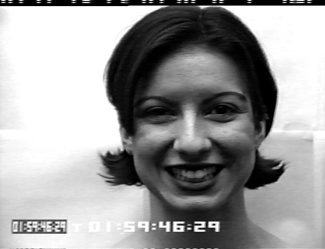
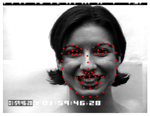
Figure 1: An element of the CK+ dataset: happy face (left) and its point cloud (right).

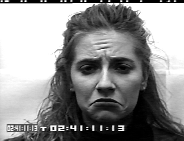
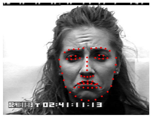
Figure 2: An element of the CK+ dataset: sad face (left) and its point cloud (right).

From this point cloud we select only those 20 points associated to the mouth as shown in Fig. 3 for the happy expression.

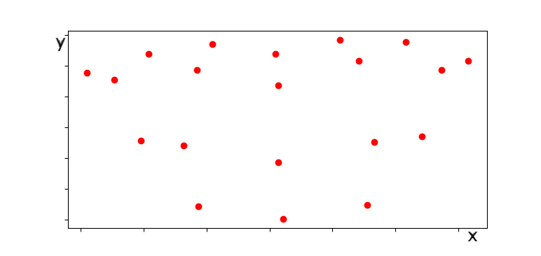
Figure 3: Landmark points associated to the happy mouth. Points are represented in the (x,y) plane.

With the objective of using this dataset for the inputs of a quantum circuit implementing a classifier of expressions, we first associate a graph to each object of the data set by following two alternative strategies.

The first strategy considers the weighted complete graph whose vertices are the $n$ landmark points of the mouth and whose edge-weights $w_{\_}{ij}$ correspond to the Euclidean distance of vertex $i$ from vertex $j$. Since a complete graph with $n$ vertices has $n(n-1)/2$ edges, its construction requires $O(n^{2})$ steps.

The second strategy is based on the Delaunay triangulation of a set $S$ of $n$ points in $\mathbb{R}^{2}$ [3]. This is a technique for subdividing a planar object into triangles (and a general geometric object in $\mathbb{R}^{d}$ into simplices), which constructs a partition of $\mathbb{R}^{2}$ in triangles (or polyhedral in $\mathbb{R}^{d}$) as follows: for each point $p$ in the set $S$, consider the convex hulls of the set of points that are closer to $p$ than to any other point in $S$, with respect to the Euclidean distance; then take all the convex hulls together with their faces. The most straightforward algorithm finds the Delaunay triangulation of a set of $n$ points in $O(n^{2})$ by randomly adding one vertex at a time and triangulating again the affected parts of the graph. However, it is possible to improve this algorithm and reduce the runtime to $O(n\log n)$ as shown in [7]. By applying the Delaunay triangulation to the points of the mouth of the facial expressions, we obtain meshed weighted graphs, where weights are the same as those used for the complete graphs.

Given a mouth landmark point cloud as in Fig.3, the outputs of these two strategies are shown in Figure 4.

Complete graph

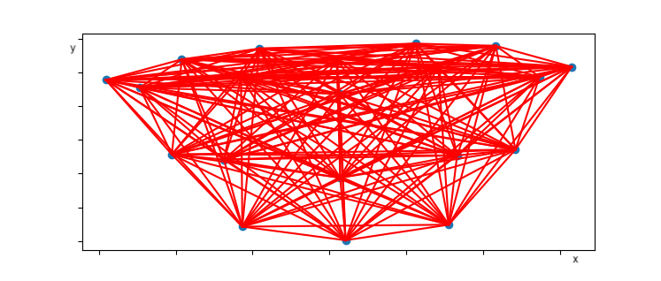
Meshed graph

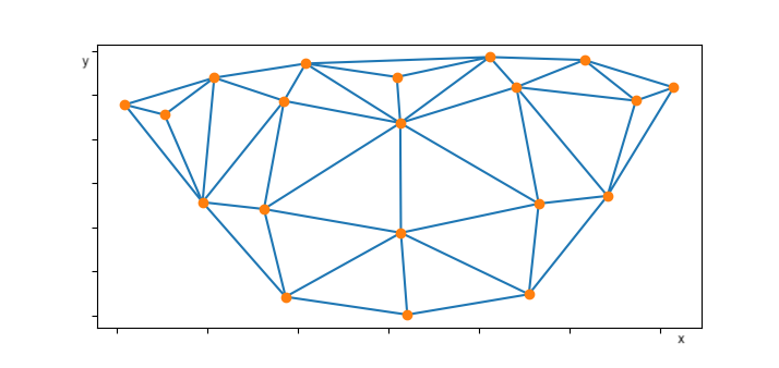
Figure 4: Complete and meshed graphs obtained from the mouth landmark points of the happy face, using all the 20 nodes that identify the mouth.

Clearly, one can expect that a classification based on the complete graphs strategy gives a higher accuracy than the meshed one, as it can exploit a richer description of the data. As we will see later, although this is true for the classical case, the quantum algorithm we present may achieve a better accuracy with the meshed strategy, due to a lower error rate occurring in this case (matrices are sparser than those for complete graphs).

3 Encoding Graphs into Quantum States

Consider an undirected simple graph $G=(V_{\_}G,E_{\_}G)$, where $V_{\_}G$ is the set of vertices and $E_{\_}G$ the set of edges in $G$. By fixing an ordering of the vertices $\{v_{\_}i\}_{\_}{i=1,..n}$, a graph $G$ is uniquely identified by its adjacency matrix $A_{\_}G$ with generic element

$$a_{\_}{ij}=\begin{cases}1&\text{if }e_{\_}{ij}\in E_{\_}G,\\ 0&\text{if }e_{\_}{ij}\notin E_{\_}G.\end{cases}$$

Therefore if the cardinality of $V_{\_}G$ is $n$, i.e. the graph G has n vertices, then $A_{\_}G$ is a n$\times$n square matrix with zeros on the diagonal. Since we are dealing with undirected simple graphs, $A_{\_}G$ is also symmetric and this means that the meaningful information about graph $G$ is contained in the $d=(n^{2}-n)/2$ elements of the upper triangular part of $A_{\_}G$. We can now vectorize those elements and rename them as follows:

$$\mathbf{a}_{\_}G=\left(a_{\_}{12},a_{\_}{13},..,a_{\_}{1n},a_{\_}{23},..,a_{\_}{2n},..,a_{\_}{(n-1)n}\right)^{T}=\left(g^{(G)}_{\_}1,g^{(G)}_{\_}2,..,g^{(G)}_{\_}{d}\right)^{T}$$ (1)

where

$$g^{(G)}_{\_}{k}\equiv a_{\_}{i,j}\mbox{ for }k=i\times n-\frac{i(i+1)}{2}-n+j.$$

Following the approach in [15], from vector $\mathbf{a}_{\_}G$ we construct a quantum state $|G\rangle$ associated to graph $G$ by encoding the elements of the adjacency vector into the amplitudes of the quantum state:

$$|G\rangle=\dfrac{1}{\gamma}\sum_{\_}{k=1}^{d}g_{\_}k|k\rangle,$$ (2)

where $\gamma$ is a normalization constant given by

$$\gamma=\sqrt{\sum_{\_}{\{k\ \mathrm{s.t}.\ g_{\_}k\neq 0\}}|g_{\_}k|^{2}}.$$ (3)

This encoding can be extended to the case of weighted graphs $G=(V_{\_}G,E_{\_}G,w_{\_}{ij})$, where $w_{\_}{ij}\in\mathbb{R}_{\_}{\geq 0}$ is the weight associated to the edge $e_{\_}{ij}\in E_{\_}G$. In this case, the adjacency matrix is defined as

$$a_{\_}{ij}=\begin{cases}w_{\_}{ij}&\text{if }e_{\_}{ij}\in E_{\_}G,\\ 0&\text{if }e_{\_}{ij}\notin E_{\_}G.\end{cases}$$

Quantum state encoding is then performed as in Equations (1), (2), (3). This allows us to represent a classical vector of $d$ elements into a quantum state of $N=\lceil\log(d)\rceil$ qubits, i.e., in our case, with a number of qubits that grows linearly with the number $n$ of the graph vertices.

On the IBM Qiskit framework [1], states expressed by Equation (2) are realized by using a method proposed by Shende et al. in [19]. This method is based on an asymptotically-optimal algorithm for the initialization of a quantum register, which exploits the fact that an arbitrary $n$-qubit state can be decomposed into a separable (i.e. unentangled) state by applying the two controlled rotation $\mathbf{R_{\_}z}$ and $\mathbf{R_{\_}y}$. By recursively applying this transformation to the $n$-qubit register with the desired target state (i.e. $|G\rangle$, in our case), we can construct a circuit that takes it to the $n$-qubit $|00...0\rangle$ state. This can be done using a quantum multiplexor circuit $\mathbf{U}$, which is finally reversed in order to get the desired initialization circuit. In our case, we identify such an initialization circuit with the unitary $\mathbf{G}$ that manipulates a register of $N$ qubits initially in $|0\rangle$ as follows:

$$\mathbf{G}|00...0\rangle=|G\rangle,$$

where $\mathbf{G}$ represents the following circuit with elementary components $CX$, $R_{\_}y(\theta)$ and $R_{\_}z(\phi)$:

$$\mathbf{G}=\begin{bmatrix}R_{\_}y(-\theta_{\_}0)R_{\_}z(-\phi_{\_}0)&&&\\ &R_{\_}y(-\theta_{\_}1)R_{\_}z(-\phi_{\_}1)&&\\ &&\ddots&\\ &&&R_{\_}y(-\theta_{\_}{2^{N-1}-1})R_{\_}z(-\phi_{\_}{2^{N-1}-1})\end{bmatrix}^{{\dagger}}$$

Unfortunately, the construction of $\mathbf{G}$ in this way requires $O(2^{N+1})$ gates, thus representing a bottleneck for our algorithm. It will be the subject of future work to try different state preparation schemes by investigating other approaches such as those in [13, 10, 2, 21, 13, 6].

3.1 An Example

Let’s select $n=4$ random vertices among those belonging to the mouth landmark points. The complete graph constructed for these points looks like the one in Fig. 5.

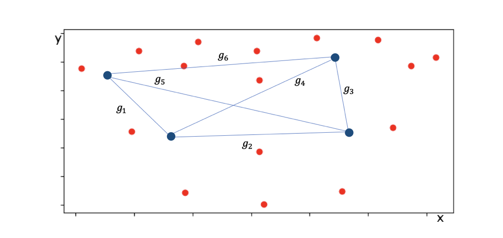
Figure 5: Complete graph with four randomly selected mouth landmark points.

Such a graph is encoded into the quantum state $|G_{\_}4\rangle$ defined by

$$|G_{\_}4\rangle=\dfrac{1}{\gamma}\left(g_{\_}1|000\rangle+g_{\_}2|001\rangle+g_{\_}3|010\rangle+g_{\_}4|011\rangle+g_{\_}5|100\rangle+g_{\_}6|101\rangle\right),$$

where $\gamma$ is a normalization constant. The quantum circuit $\mathbf{G_{\_}4}$ that realizes $|G_{\_}4\rangle$, i.e. such that $\mathbf{G_{\_}4}|000\rangle=|G_{\_}4\rangle$, via the method proposed by Shende et al. in [19] is shown in Fig.6, where the gate $\mathbf{U(\theta)}$ is defined by

$$\mathbf{U(\theta)}=\begin{bmatrix}\cos(\theta/2)&\ \ \ -\sin(\theta/2)\\ \sin(\theta/2)&\ \ \ \cos(\theta/2)\end{bmatrix}$$

$$\Qcircuit@C=.5em@R=0.5em@!R{&\lstick{a:|0\rangle}\qw\qw\qw\qw\qw\qw\qw\qw\qw\qw\qw\gate{\mathbf{X}}\qw\ >\\ \lstick{b:|0\rangle}\qw\qw\qw\gate{\mathbf{X}}\qw\gate{\mathbf{U(0.7854)}}\qw\gate{\mathbf{X}}\qw\gate{\mathbf{U(0.7854)}}\qw\qw\qw\ >\\ \lstick{c:|0\rangle}\qw\gate{\mathbf{U(1.231)}}\qw\ctrl{-1}\qw\qw\qw\ctrl{-1}\qw\qw\qw\ctrl{-2}\qw\ >}$$

$$\Qcircuit@C=.5em@R=0.5em@!R{&\lstick{a:}\qw\gate{\mathbf{U(0.3927)}}\qw\gate{\mathbf{X}}\qw\gate{\mathbf{U(-0.3927)}}\qw\gate{\mathbf{X}}\qw\gate{\mathbf{X}}\qw\gate{\mathbf{X}}\qw\qw\ >\\ \lstick{b:}\qw\qw\qw\ctrl{-1}\qw\qw\qw\ctrl{-1}\qw\qw\qw\ctrl{-1}\qw\qw\ >\\ \lstick{c:}\qw\qw\qw\qw\qw\qw\qw\qw\qw\ctrl{-2}\qw\qw\qw\qw\ >}$$

$$\Qcircuit@C=.5em@R=0.5em@!R{&\lstick{a:}\qw\gate{\mathbf{U(0.3927)}}\qw\gate{\mathbf{X}}\qw\gate{\mathbf{U(1.1781)}}\qw\gate{\mathbf{X}}\qw\gate{\mathbf{X}}\qw\qw\\ \lstick{b:}\qw\qw\qw\ctrl{-1}\qw\qw\qw\qw\qw\ctrl{-1}\qw\qw\\ \lstick{c:}\qw\qw\qw\qw\qw\qw\qw\ctrl{-2}\qw\qw\qw\qw}$$

Figure 6: Quantum circuit constructing the state $\mathbf{G_{\_}4}$. Three qubits are employed in the circuit, which are denoted by $a$, $b$ and $c$.

As claimed before, this algorithm is exponential in the number of the input qubits and represents a bottleneck to the speed of the whole algorithm. Thus, finding a more efficient encoding of the data into quantum states is crucial for achieving a better performance of the overall algorithm we are going to define in the next section. This would also benefit from a more complex connection between physical qubits in the hardware that would allow us to reduce the number of swap gates used to adapt the quantum circuit to the topology of the quantum computer.

4 Graphs Quantum Classifier

The first implementation of a quantum classifier on the IBM quantum computer appears in [16], where data are encoded in a single qubit state. We extend the work in that paper by constructing a circuit that is able to deal with multiple qubit state representations of a dataset.

Given a dataset $\mathcal{D}$, consider the training set,

$$\mathcal{D}_{\_}{train}=\{(G^{\left\{1\right\}},y^{\left\{1\right\}}),...,(G^{\left\{M\right\}},y^{\left\{M\right\}})\},$$

of $M$ pairs $(G^{\left\{m\right\}},y^{\left\{m\right\}})$, where $G^{\left\{m\right\}}$ are graphs (e.g. representing the face of an individual) while $y^{\left\{m\right\}}\in\{c_{\_}l\}_{\_}{l=1}^{L}$ identify which of the $L$ possible class labels are associated to a graph. Classes partition graphs according to some features, which in our case correspond to sad vs happy face expressions.

Given a new unlabeled input $G_{\_}{test}$, the task is to assign a label ${y_{\_}{test}}$ to $G_{\_}{test}$ using the distance

$$d(G_{\_}1,G_{\_}2)=\sqrt{|\mathbf{a}_{\_}{G_{\_}{1}}-\mathbf{a}_{\_}{G_{\_}2}|^{2}}=\sqrt{\sum_{\_}{i=1}^{d}\left|g_{\_}i^{(G_{\_}{1})}-g_{\_}i^{(G_{\_}2)}\right|^{2}},$$

and then classifying according to

$$\min_{\_}{c_{\_}l}\left[\sum\limits_{\_}{m\ s.t.\ y^{\left\{m\right\}}=c_{\_}l}d\left(G_{\_}{test},G^{\left\{m\right\}}\right)\right].$$ (4)

In the case of binary classification, where there are only two classes, i.e. $y^{\left\{m\right\}}\in\{+1,-1\}$, the classifier of Equation (4) can be expressed as

$$y_{\_}{test}=-\mathrm{sgn}\left[\sum\limits_{\_}{m=1}^{M}y^{\left\{m\right\}}d\left(G_{\_}{test},G^{\left\{m\right\}}\right)\right].$$ (5)

The quantum circuit that implements such a classification requires four multi-qubit quantum registers. In the initial configuration,

• $|0\rangle_{\_}a$ is an ancillary qubit that is entangled to the qubits encoding both the test graph and the training graphs;

• $|00..0\rangle_{\_}m$ is a register of $\lceil\log(M)\rceil$ qubits that stores the index $m$ of the training graphs $G^{\left\{m\right\}}$;

• $|00..0\rangle_{\_}g$ is a register of $\lceil\log(d)\rceil$ qubits used to encode both test and training graphs;

• $|00..0\rangle_{\_}c$ is a register of $\lceil\log(L)\rceil$ qubits that stores the classes $y^{\left\{m\right\}}\in\{c_{\_}l\}_{\_}{l=1}^{L}$ of the $G^{\left\{m\right\}}$.

In the case of a training set of two graphs, one per class, the circuit is implemented as shown in Fig. (7).

$$\Qcircuit@C=.5em@R=0.5em@!R{&\lstick{|0\rangle_{\_}a}\qw\gate{\mathbf{H}}\qw\qw\ctrl{2}\gate{\mathbf{X}}\qw\qw\ctrl{1}\qw\qw\qw\ctrl{1}\qw\qw\qw\gate{\mathbf{H}}\qw\meter\cw\cctrlo{3}\rstick{a}\cw\\ \lstick{|0\rangle_{\_}m}\qw\gate{\mathbf{H}}\qw\qw\qw\qw\qw\qw\ctrl{1}\gate{\mathbf{X}}\qw\qw\ctrl{1}\qw\qw\ctrl{2}\qw\qw\qw\qw\qw\qw\\ \lstick{|00..0\rangle_{\_}g}\qw\qw\qw\qw\gate{\mathbf{G_{\_}{test}}}\qw\qw\qw\gate{\mathbf{G^{\left\{1\right\}}}}\qw\qw\qw\gate{\mathbf{G^{\left\{2\right\}}}}\qw\ \qw\qw\qw\qw\qw\qw\qw\qw\\ \lstick{|0\rangle_{\_}c}\qw\qw\qw\qw\qw\qw\qw\qw\qw\qw\qw\qw\qw\qw\qw\targ\qw\qw\qw\qw\qw\meter\rstick{c}\cw\ }$$

Figure 7: Quantum binary classifier circuit.

After the first two Hadamard gates, the circuit is in state

$$\dfrac{1}{2}\left(|0\rangle_{\_}a+|1\rangle_{\_}a\right)\left(|0\rangle_{\_}m+|1\rangle_{\_}m\right)|00..0\rangle_{\_}g|0\rangle_{\_}c.$$

The $\mathbf{Control}$-$\mathbf{G_{\_}{test}}$ gate, followed by an $\mathbf{X}$ operator on the ancilla produces the state

$$|G_{\_}{test}\rangle=\dfrac{1}{\gamma_{\_}{test}}\sum_{\_}{k=1}^{d}g_{\_}k^{test}|k\rangle,$$

and entangles it with the $|0\rangle_{\_}a$ state of the ancilla. Then a $\mathbf{G^{\left\{1\right\}}}$ gate is controlled by both the first qubit $a$ and by the second one $m$, which is also subjected to an $\mathbf{X}$ gate afterwards. This has the effect of creating the state associated to the training graph $G^{\left\{1\right\}}$, namely

$$|G^{\left\{1\right\}}\rangle=\dfrac{1}{\gamma^{\left\{1\right\}}}\sum_{\_}{k=1}^{d}g_{\_}k^{\left\{1\right\}}|k\rangle,$$

and entangling it with both $|1\rangle_{\_}a$ and $|0\rangle_{\_}m$. Then, the double controlled $\mathbf{G^{\left\{2\right\}}}$ gate has a similar effect, entangling the second training graph state $|G^{\left\{2\right\}}\rangle$ with $|1\rangle_{\_}a$ and $|1\rangle_{\_}m$. At this stage, the $\mathbf{Control}$-$\mathbf{X}$ gate entangles the $m$ index of the two test graphs with the correct class state, i.e. either $|0\rangle_{\_}c$ or $|1\rangle_{\_}c$. The state of the circuit at this point can be written as

$$\frac{1}{\sqrt{2M}}\sum_{\_}{m=0}^{M-1}\Big{(}|0\rangle_{\_}a|G_{\_}{test}\rangle_{\_}g+|1\rangle_{\_}a|G^{\left\{m\right\}}\rangle_{\_}g\Big{)}|m\rangle_{\_}m\ |y^{\left\{m\right\}}\rangle_{\_}c.$$

Finally, the Hadamard gate applied to the ancilla generates the state

$$\frac{1}{2\sqrt{M}}\sum_{\_}{m=0}^{M-1}\Big{[}|0\rangle_{\_}a\left(|G_{\_}{test}\rangle_{\_}g+|G^{\left\{m\right\}}\rangle_{\_}g\right)+|1\rangle_{\_}a\left(|G_{\_}{test}\rangle_{\_}g-|G^{\left\{m\right\}}\rangle_{\_}g\right)\Big{]}|m\rangle_{\_}m\ |y^{\left\{m\right\}}\rangle_{\_}c.$$

Measuring the ancilla in the state $|0\rangle_{\_}a$ produces the state

$$\frac{1}{\sqrt{\sum_{\_}m\sum_{\_}i|g_{\_}i^{(G_{\_}{test})}+g_{\_}i^{(G^{\left\{m\right\}})}|^{2}}}\sum_{\_}{m=0}^{M-1}\sum_{\_}{i=1}^{d}\left(g_{\_}i^{(G_{\_}{test})}+g_{\_}i^{(G^{\left\{m\right\}})}\right)|i\rangle_{\_}g\ |m\rangle_{\_}m\ |y^{\left\{m\right\}}\rangle_{\_}c,$$

and a subsequent measurement of the class qubit $|y^{\left\{m\right\}}\rangle$ gives the outcome corresponding to state $|0\rangle_{\_}c$ with probability

$$\begin{split}\mathrm{p}(y^{\left\{m\right\}}=0)=\frac{1}{{\sum_{\_}m\sum_{\_}i|g_{\_}i^{(G_{\_}{test})}+g_{\_}i^{(G^{\left\{m\right\}})}|^{2}}}\sum\limits_{\_}{m\ s.t.\ y^{\left\{m\right\}}=0}\ \sum_{\_}{i=1}^{d}\left|g_{\_}i^{(G_{\_}{test})}+g_{\_}i^{(G^{\left\{m\right\}})}\right|^{2}=\\ =1-\left(\frac{1}{{\sum_{\_}m\sum_{\_}i|g_{\_}i^{(G_{\_}{test})}+g_{\_}i^{(G^{\left\{m\right\}})}|^{2}}}\sum\limits_{\_}{m\ s.t.\ y^{\left\{m\right\}}=0}\ d(G_{\_}{test},G^{\left\{m\right\}})^{2}\right).\end{split}$$

This probability depends on the distance between the test graph $G_{\_}{test}$ and all those training graphs belonging to the class $c=0$. Therefore, if its value is lower than $0.5$, then the test set is classified as $y_{\_}{class}=-1$ while if it is higher, then the test set is classified as $y_{\_}{class}=+1$. The quantum circuit hence realizes the classification expressed by Equation (5).

5 Classification Algorithm and Experimental Results

The number of qubits used by the quantum classifier scales with the number, $n$, of vertices in the graphs, which are randomly selected among those of the mouth landmark points. As shown in Table 1 the encoding allows for an exponential compression of resources since only a number $O(log_{\_}2(n^{2}))$ of qubits are needed to represent a complete graph of $n$ nodes. In the table, the number of elements in the adjacency matrix that identify the graphs is denoted by $d$ and its value is $n(n-1)/2$.

$n$	$d\approx O(n^{2})$	$\#$ qubits used by the algorithm
3	9	7
4	16	8
5	25	8
10	100	10
20	400	12
50	2500	15
100	10000	17
500	250000	21
1$\times 10^{7}$	1$\times 10^{14}$	50

Table 1: Input size of the classification circuit depending on the number of vertices.

We evaluated our quantum classifier on both the complete and the meshed graphs using the qasm_simulator available through the IBM cloud platform. We compared the results with a classical binary classifier based on the Fröbenius norm between graph adjacency matrices defined by

$$||A||=\sqrt{\sum_{\_}{i,j}|a_{\_}{ij}|^{2}},$$

so that the distance used in Equation (5) becomes

$$d\left(G_{\_}{test},G^{\left\{m\right\}}\right)=\sqrt{\sum_{\_}{ij}{|(g_{\_}i^{test}-g_{\_}i^{\{m\}})|}^{2}}.$$ (6)

In order to perform our experiments, we proceeded as follows. By randomly selecting 10 different test graphs $G_{\_}\text{test}$ and 25 different pairs of labeled graphs $\left\{G_{\_}\text{sad},G_{\_}\text{happy}\right\}$, we constructed 250 items of the form $\left\{G_{\_}\text{test},G_{\_}\text{sad},G_{\_}\text{happy}\right\}$ for the classical classifier and the IBM quantum simulator. Vertices were selected randomly among the 20 landmark points of the mouth, the number $n$ of vertices given in input to the algorithm was gradually increased, and a one-time sample of the vertices was shared with all methods.

Based on this, we have devised an algorithm for classification that is divided into two main steps. The first step consists in a procedure, named ClassifyWrtSingleFace, that considers each item $\left\{G_{\_}\text{test},G_{\_}\text{sad},G_{\_}\text{happy}\right\}$ individually and classifies $G_{\_}{test}$ as happy or sad, based only on the distances $d(G_{\_}\text{test},G_{\_}\text{sad})$ and $d(G_{\_}\text{test},G_{\_}\text{happy})$. The procedure AccuracyWrtSingleFace evaluates the accuracy of such a classification by essentially counting the number of correct answers for all the test graphs. In the second step, another procedure, named ClassifyWrtWholeSet, performs a different classification where each face $G_{\_}\text{test}$ is labeled depending on the output of ClassifyWrtSingleFace calculated on the whole set $\{G_{\_}\text{happy},G_{\_}\text{sad}\}$.

We have compared the accuracy obtained with different number $n$ of landmark points of the mouth ranging from $4$ to $20$. The $20$ points case considers all the points of the mouth. The $n<20$ cases consider subsets of the mouth landmark points which are chosen randomly and uniformly in the coordinates. For each $n$ we have picked up 20 randomly chosen subsets, and we have calculated the accuracy of the classifier for each $n$ as the mean of the accuracies obtained by varying such subsets.

5.1 Algorithm Step 1

1:procedure ClassifyWrtSingleFace($G_{\_}\text{test},G_{\_}\text{sad},G_{\_}\text{happy}$)

2:     $d\leftarrow\textsc{Distance}(G_{\_}\text{test},G_{\_}\text{sad})-\textsc{Distance}(G_{\_}\text{test},G_{\_}\text{happy})$

3:     if abs($d$) < 0.001 then

4:         return unknown

5:     end if

6:     if $d$ < 0 then

7:         return happy

8:     else

9:         return sad

10:     end if

11:end procedure

The evaluation of the distance is obtained classically via the calculation of Equation (6), and quantumly via the application of the circuit to the item $\{G_{\_}\text{test},G_{\_}\text{sad},G_{\_}\text{happy}\}$. The circuit is executed 1024 times.

Given the set of all test graphs $\mathcal{G}=\{(G_{\_}i,\ell_{\_}i)\mid i=1,...,n\}$, the following procedure describes the calculation of the accuracy of the classification with respect to a single face.

1:procedure CalculateAccuracyWrtSingleFace($\mathcal{G}$)

2:     correct $\leftarrow 0$

3:     wrong $\leftarrow 0$

4:     $\mathcal{G}_{\_}\text{sad}=\{G\mid(G,\ell)\in\mathcal{G}\land\ell=\text{sad}\}$

5:     $\mathcal{G}_{\_}\text{happy}=\{G\mid(G,\ell)\in\mathcal{G}\land\ell=\text{happy}\}$

6:     for all $(G_{\_}\text{test},\ell_{\_}\text{test})\in\mathcal{G}$ do

7:         for all $G_{\_}\text{sad}\in\mathcal{G}_{\_}\text{sad}$, $G_{\_}\text{happy}\in\mathcal{G}_{\_}\text{happy}$ do

8:              if $\textsc{ClassifyWrtSingleFace}(G_{\_}\text{test},G_{\_}\text{sad},G_{\_}\text{happy})=\ell_{\_}\text{test}$ then

9:                  correct $\leftarrow$ correct $+1$

10:              else

11:                  wrong $\leftarrow$ wrong $+1$

12:              end if

13:         end for

14:     end for

15:     AccuracyWrtSingleFace $\leftarrow$ correct$/($correct$+$wrong$)$

16:     return AccuracyWrtSingleFace

17:end procedure

The values of the accuracy of procedure ClassifyWrtSingleFace that we obtained with the qasm_simulator are reported in Table 2 and described by the plot in Fig. 8.

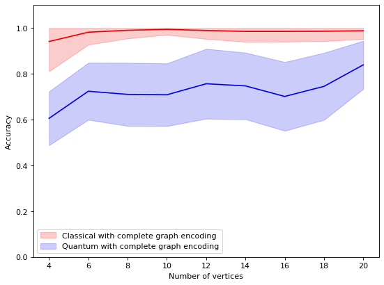
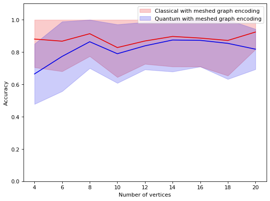
Figure 8: Results of the procedure AccuracyWrtSingleFace on graphs with number of vertices $n\in[4,20]$, obtained with the qasm_simulator compared with the classical classifier. Plots show the average accuracy of the classifiers with shadow indicating the max and min accuracies.

$n$	CC meshed	CC complete	QC meshed	QC complete
4	0.88	0.94	0.66	0.61
6	0.87	0.98	0.77	0.72
8	0.91	0.99	0.86	0.71
10	0.83	0.99	0.79	0.71
12	0.87	0.99	0.84	0.76
14	0.90	0.98	0.87	0.75
16	0.89	0.98	0.87	0.70
18	0.87	0.99	0.85	0.75
20	0.92	0.99	0.82	0.84

Table 2: Average accuracy of the ClassifyWrtSingleFace procedure obtained with the qasm_simulator (QC), and the classical classifier (CC).

Fig. 8 and Table 2 show that the highest value of the AccuracyWrtSingleFace procedure is obtained with the classical classifier, using the complete graph strategy. The classical classifier with meshed graphs reveals a worse performance. This is due to the fact that meshed graphs, on average, carry less information about the shape of the mouth. The performance gap between the complete and meshed approach is not so evident for what concerns the quantum simulation. This may be due to the fact that the encoding of a complete graph into a quantum state is much more complex than for meshed graphs since for complete graphs there are always $n(n-1)/2$ amplitudes that are different from zero. In the meshed case, the graphs are sparse and much less amplitudes are needed in the quantum states for encoding them. Clearly, the complexity of the quantum states negatively affects the robustness of the circuit. Moreover, it is interesting to notice how the accuracy of the quantum simulation with meshed graphs closely follows the trend of the accuracy obtained by its classical counterpart.

5.2 Algorithm Step 2

We now refine the classification by comparing $G_{\_}\text{test}$ with the entire set of graphs, $\{G_{\_}\text{happy},G_{\_}\text{sad}\}$, so that a face is classified as happy if by running procedure ClassifyWrtSingleFace we obtain more times happy than sad, and sad otherwise.

The ClassifyWrtWholeSet procedure is described below.

1:procedure ClassifyWrtWholeSet($G_{\_}\text{test},\mathcal{G}$)

2:     happycounter $\leftarrow 0$

3:     sadcounter $\leftarrow 0$

4:     $\mathcal{G}_{\_}\text{sad}=\{G\mid(G,\ell)\in\mathcal{G}\land\ell=\text{sad}\}$

5:     $\mathcal{G}_{\_}\text{happy}=\{G\mid(G,\ell)\in\mathcal{G}\land\ell=\text{happy}\}$

6:     for all $G_{\_}\text{sad}\in\mathcal{G}_{\_}\text{sad}$, $G_{\_}\text{happy}\in\mathcal{G}_{\_}\text{happy}$ do

7:         if $\textsc{ClassifyWrtSingleFace}(G_{\_}\text{test},G_{\_}\text{sad},G_{\_}\text{happy})=\text{happy}$ then

8:              happycounter $\leftarrow$ happycounter $+1$

9:         else

10:              sadcounter $\leftarrow$ sadcounter $+1$

11:         end if

12:     end for

13:     if happycounter$==$sadcounter then

14:         return unknown

15:     end if

16:     if happycounter$>$sadcounter then

17:         return happy

18:     else

19:         return sad

20:     end if

21:end procedure

The accuracy of the above procedure is calculated by the following algorithm as the frequency of the correct answers returned by the ClassifyWrtWholeSet procedure.

1:procedure CalculateAccuracyWholeSet($\mathcal{G}$)

2:     correct $\leftarrow 0$

3:     wrong $\leftarrow 0$

4:     for all $(G_{\_}\text{test},\ell_{\_}\text{test})\in\mathcal{G}$ do

5:         if $\textsc{ClassifyWrtWholeSet}(G_{\_}\text{test},\mathcal{G})=\ell_{\_}\text{test}$ then

6:              correct $\leftarrow$ correct $+1$

7:         else

8:              wrong $\leftarrow$ wrong $+1$

9:         end if

10:     end for

11:     AccuracyWholeSet $\leftarrow$ correct$/($correct$+$wrong$)$

12:     return AccuracyWholeSet

13:end procedure

The values returned by the CalculateAccuracyWholeSet procedure for the qasm_simulator and the classical binary classifier are shown in Fig. 9 and Table 3.

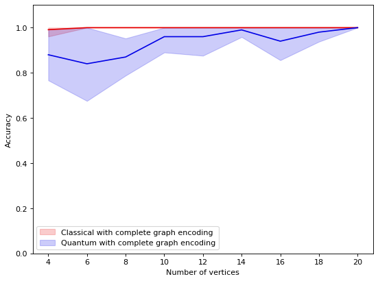
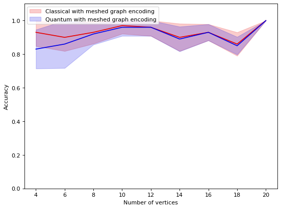
Figure 9: Results of the procedure AccuracyWholeSet on graphs with number of vertices $n\in[4,20]$, obtained with the qasm_simulator compared with the classical classifier. Plots show the average accuracy of the classifiers with shadow indicating the max and min accuracies.

$n$	CC meshed	CC complete	QC meshed	QC complete
4	0.93	0.99	0.83	0.88
6	0.90	1.0	0.86	0.84
8	0.93	1.0	0.92	0.87
10	0.97	1.0	0.96	0.96
12	0.96	1.0	0.96	0.96
14	0.90	1.0	0.89	0.99
16	0.93	1.0	0.93	0.94
18	0.86	1.0	0.85	0.98
20	1.0	1.0	1.0	1.0

Table 3: Results of the average AccuracyWholeSet procedure on graphs with number of vertices $n\in[4,20]$, obtained with the qasm_simulator (QC) and the classical classifier (CC).

As in Step 1, the highest value of the accuracy is obtained with the classical classifier using the complete graph strategy: the fact that all distances between landmark points are considered makes the classifier very faithful. However, it is worth noticing that we only considered small graphs (up to 20 nodes), thus reducing the amount of resources needed to deal with large complete graphs. In applications where graph dimensions are several orders of magnitude higher, a complete graph classification approach may not be a viable option.

A trade-off between graph complexity and accuracy of the classification is reached in the classical case by employing the meshed graphs encoding; good levels of accuracy are obtained with our AccuracyWholeSet algorithm, which never go below $0.86$.

In the quantum simulation, the complete graph strategy performs clearly worse than its classical counterpart, while the quantum meshed approach shows an average accuracy which is very close to the classical one.

Comparing Fig. 9 and Fig. 8, we can also observe that in the latter, the quantum complete graph strategy has a smaller deviation (blue shadows in Fig.8 ) than for the quantum meshed graph approach; this is not the case for AccuracyWholeSet, where we achieve comparable results.

6 Conclusion

In this work we have addressed the problem of classifying graphs representing human facial expressions. Graphs are obtained by selecting some of the face landmark points and connecting them either via a triangulation of the points or via a complete graph construction. We have shown the construction of quantum states whose amplitudes encode the graphs, and devised an interference-based quantum circuit that performs a distance-based classification for the encoded graphs. We have implemented this quantum circuit by means of the IBM open-source quantum computing framework Qiskit [1], and tested it on a collection of images taken from the Cohn-Kanade (CK) database, one of the most widely used test-beds for algorithm development and evaluation in the field of automatic facial expressions recognition.

The tests have been performed on the qasm_simulator, and the results have been compared with the classical classifier. A calculation of the accuracy revealed that the classical classifier achieves better results when a complete graph approach is employed, while the simulated quantum classifier achieves comparable results with both the meshed and the complete strategy.

Future work should investigate the possibilities of different and more efficient graph encodings into quantum states. Moreover, interesting extensions of the results we have presented could be obtained by exploiting other quantum classification schemes, such as those based on the SWAP test along the lines of [12], or on Variational Quantum Circuits [9].

References

- [1] Aleksandrowicz, G., Alexander, T., Barkoutsos, P., Bello, L., Ben-Haim, Y., Bucher, D., …, Zoufal, C.: Qiskit: An Open-source Framework for Quantum Computing (2019). doi:10.5281/zenodo.2562110
- [2] Arunachalam, S., Gheorghiu, V., Jochym-O’Connor, T., Mosca, M., Srinivasan, P.V.: On the robustness of bucket brigade quantum RAM. New Journal of Physics 17(12) (2015). doi:10.1088/1367-2630/17/12/123010
- [3] de Berg, M., van Kreveld, M., Overmars, M., Schwarzkopf, O.C.: Delaunay Triangulations, pp. 183–210. Springer (2000). doi:10.1007/978-3-662-04245-8_9
- [4] Biamonte, J., Wittek, P., Pancotti, N., Rebentrost, P., Wiebe, N., Lloyd, S.: Quantum machine learning. Nature 549, 195–202 (2017). doi:doi.org/10.1038/nature23474
- [5] Bondy, J.A.: Graph Theory With Applications. Elsevier Science (1976)
- [6] Ciliberto, C., Herbster, M., Ialongo, A.D., Pontil, M., Rocchetto, A., Severini, S., Wossnig, L.: Quantum machine learning: a classical perspective. Proceedings of the Royal Society A: Mathematical, Physical and Engineering Sciences 474(2209), 20170551 (2018). doi:10.1098/rspa.2017.0551
- [7] de Berg, M., Cheong, O., van Kreveld, M., Overmars, M.: Computational Geometry: Algorithms and Applications. Springer-Verlag Berlin Heidelberg (2008)
- [8] Lucey, P., Cohn, J.F., Kanade, T., Saragih, J., Ambadar, Z., Matthews, I.: The Extended Cohn-Kanade Dataset (CK+): A complete dataset for action unit and emotion-specified expression. In: 2010 IEEE Computer Society Conference on Computer Vision and Pattern Recognition – Workshops, pp. 94–101 (2010). doi:10.1109/CVPRW.2010.5543262
- [9] McClean, J.R., Romero, J., Babbush, R., Aspuru-Guzik, A.: The theory of variational hybrid quantum-classical algorithms. New Journal of Physics 18(2), 023023 (2016). doi:10.1088/1367-2630/18/2/023023
- [10] Mottonen, M., Vartiainen, J.J., Bergholm, V., Salomaa, M.M.: Transformation of quantum states using uniformly controlled rotations. Quant. Inf. Comp. 5(467) (2005)
- [11] Nielsen, M.A., Chuang, I.L.: Quantum Computation and Quantum Information, 10th anniversary edn. Cambridge University Press (2011)
- [12] Park, D.K., Blank, C., Petruccione, F.: The theory of the quantum kernel-based binary classifier. Physics Letters A p. 126422 (2020). doi:10.1016/j.physleta.2020.126422
- [13] Park, D.K., Petruccione, F., Rhee, J.K.K.: Circuit-Based Quantum Random Access Memory for Classical Data. Scientific Reports 9(1), 3949 (2019). doi:10.1038/s41598-019-40439-3
- [14] Piatokowska, E., Martyna, J.: Computer recognition of facial expressions of emotion. In: P. P. (ed.) Machine Learning and Data Mining in Pattern Recognition. MLDM 2012, Lecture Notes in Computer Science, vol. 8862. Springer, Berlin, Heidelberg (7376). doi:10.1007/978-3-642-31537-4_32
- [15] Rebentrost, P., Mohseni, M., Lloyd, S.: Quantum support vector machine for big data classification. Phys. Rev. Lett. 113, 130503 (2014). doi:10.1103/PhysRevLett.113.130503
- [16] Schuld, M., Fingerhuth, M., Petruccione, F.: Implementing a distance-based classifier with a quantum interference circuit. EPL (Europhysics Letters) 119(6), 60002 (2017). doi:10.1209/0295-5075/119/60002
- [17] Schuld, M., Sinayskiy, I., Petruccione, F.: Quantum computing for pattern classification. In: P.S. Pham DN. (ed.) Trends in Artificial Intelligence. PRICAI 2014, Lecture Notes in Computer Science, vol. 8862. Springer, Cham (2014). doi:10.1007/978-3-319-13560-1_17
- [18] Schuld, M., Sinayskiy, I., Petruccione, F.: An introduction to quantum machine learning. Contemporary Physics 56(2), 172–185 (2015). doi:10.1080/00107514.2014.964942
- [19] Shende, V.V., Bullock, S.S., Markov, I.L.: Synthesis of quantum-logic circuits. IEEE Transactions on Computer-Aided Design of Integrated Circuits and Systems 25(6), 1000–1010 (2006). doi:10.1109/TCAD.2005.855930
- [20] Wittek, P.: Quantum Machine Learning: What Quantum Computing Means to Data Mining. Elsevier Science (2016)
- [21] Zhao, Z., Fitzsimons, J.K., Rebentrost, P., Dunjko, V., Fitzsimons, J.F.: Smooth input preparation for quantum and quantum-inspired machine learning. arXiv:1804.00281 (2018)